Introduction to Generalized Linear Models - Edps/Psych/Soc 589€¦ · Components of Generalized...

Introduction to Generalized Linear ModelsEdps/Psych/Soc 589

Carolyn J. Anderson

Department of Educational Psychology

c©Board of Trustees, University of Illinois

Fall 2019

Outline Introduction Review OLS Reg. GLM Components Random Systematic Link Natural Exponential Family of Distributions

Outline◮ Introduction (motivation and history).

◮ “Review” ordinary linear regression.

◮ Components of a GLM.

1. Random component.2. Structural component.3. Link function.

◮ Natural exponential family (technical).

◮ Normal Linear Regression re-visited.

◮ GLMs for binary data (introduction).Primary Example: High School & Beyond.

1. Linear model for π.2. Cumulative Distribution functions (alternative links).3. Logistic regression.4. Probit models.

C.J. Anderson (Illinois) Introduction to GLM Fall 2019 2.1/ 36


Outline (continued)◮ GLMs for count data.

1. Poisson regression for counts.Example: Number of deaths due to AIDs.

2. Poisson regression for rates.Example: Number of violent incidents.

◮ Inference and model checking.1. Wald, Likelihood ratio, & Score test.2. Checking Poisson regression.3. Residuals.4. Confidence intervals for fitted values (means).5. Overdispersion.

◮ Fitting GLMS (a little technical).1. Newton-Raphson algorithm/Fisher scoring.2. Statistic inference & the Likelihood function.3. “Deviance”.

◮ SummaryC.J. Anderson (Illinois) Introduction to GLM Fall 2019 3.1/ 36


Introduction to Generalized Linear Modeling

Benefits of a model that fits well:

◮ The structural form of the model describes the patterns ofinteractions or associations in data.

◮ Inference for the model parameters provides a way to evaluatewhich explanatory variable(s) are related to the responsevariable(s) while (statistically) controlling for other variables.

◮ Estimated model parameters provide measures of the strengthand (statistical) importance of effects.

◮ A model’s predicted values “smooth” the data — they providegood estimates of the mean of the response variable.



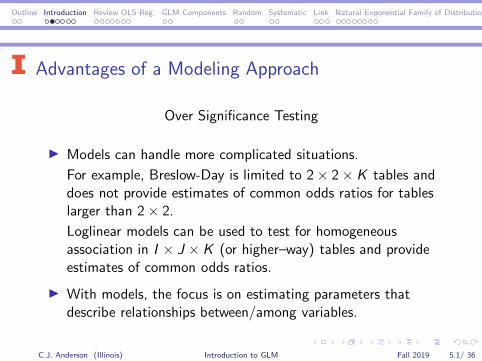
Advantages of a Modeling Approach

Over Significance Testing

◮ Models can handle more complicated situations.

For example, Breslow-Day is limited to 2× 2× K tables anddoes not provide estimates of common odds ratios for tableslarger than 2× 2.

Loglinear models can be used to test for homogeneousassociation in I × J × K (or higher–way) tables and provideestimates of common odds ratios.

◮ With models, the focus is on estimating parameters thatdescribe relationships between/among variables.



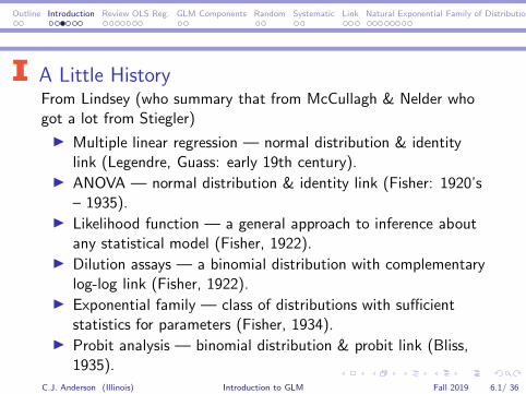
A Little HistoryFrom Lindsey (who summary that from McCullagh & Nelder whogot a lot from Stiegler)

◮ Multiple linear regression — normal distribution & identitylink (Legendre, Guass: early 19th century).

◮ ANOVA — normal distribution & identity link (Fisher: 1920’s– 1935).

◮ Likelihood function — a general approach to inference aboutany statistical model (Fisher, 1922).

◮ Dilution assays — a binomial distribution with complementarylog-log link (Fisher, 1922).

◮ Exponential family — class of distributions with sufficientstatistics for parameters (Fisher, 1934).

◮ Probit analysis — binomial distribution & probit link (Bliss,1935).



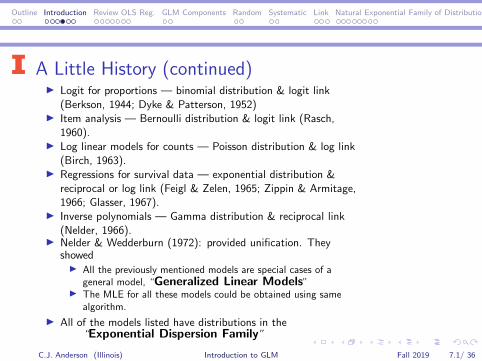
A Little History (continued)◮ Logit for proportions — binomial distribution & logit link

(Berkson, 1944; Dyke & Patterson, 1952)◮ Item analysis — Bernoulli distribution & logit link (Rasch,

1960).◮ Log linear models for counts — Poisson distribution & log link

(Birch, 1963).◮ Regressions for survival data — exponential distribution &

reciprocal or log link (Feigl & Zelen, 1965; Zippin & Armitage,1966; Glasser, 1967).

◮ Inverse polynomials — Gamma distribution & reciprocal link(Nelder, 1966).

◮ Nelder & Wedderburn (1972): provided unification. Theyshowed◮ All the previously mentioned models are special cases of a

general model, “Generalized Linear Models”◮ The MLE for all these models could be obtained using same

algorithm.

◮ All of the models listed have distributions in the“Exponential Dispersion Family”



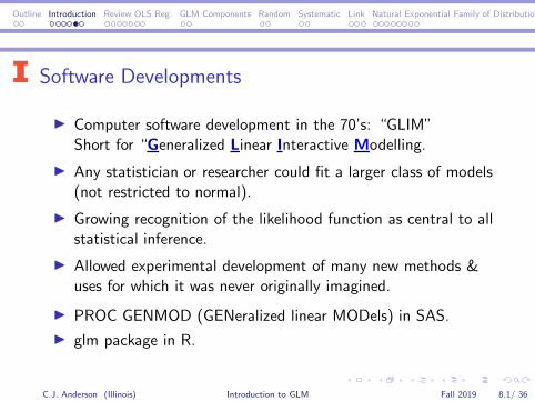
Software Developments

◮ Computer software development in the 70’s: “GLIM”Short for “Generalized Linear Interactive Modelling.

◮ Any statistician or researcher could fit a larger class of models(not restricted to normal).

◮ Growing recognition of the likelihood function as central to allstatistical inference.

◮ Allowed experimental development of many new methods &uses for which it was never originally imagined.

◮ PROC GENMOD (GENeralized linear MODels) in SAS.

◮ glm package in R.



Limitations

◮ Linear function

◮ Responses must be independent

◮ There are ways around these by going to a slightly moregeneral models and using more general software (e.g.,SAS/NLMIXED, GLIMMIX, NLP, GAMs).

◮ R has specialized packages for some of the models that are notlinear and/or dependent (e.g., packages lme4, logmult, gam).



Review of Ordinary Linear Regression

Linear (in the parameters) model for continuous/numericalresponse variable (Y ) and continuous and/or discrete explanatoryvariables (X ’s).

Yi = α+ β1x1i + β2x2i + ei

whereei ∼ N (0, σ2) and independent.

This linear model includes

◮ Multiple regression

◮ ANOVA

◮ ANCOVA



Simple Linear Regression

Yi = α+ βxi + ei

where ei ∼ N (0, σ2) and independent.

We consider X as fixed, so Yi ∼ N (µ(xi ), σ2).

In regression, the focus is on the mean or expected value of Y , i.e.,

E (Yi ) = E (α+ βxi + ei )

= α+ βxi + E (ei )

= α+ βxi



GLMs go beyond Simple Linear RegressionGeneralized Linear Models go beyond this in two major respects:

◮ The response variable(s) can have a distribution other thannormal — any distribution within a class of distributionsknown as “exponential family of distributions”.

◮ The relationship between the response (Y ) and explanatoryvariables need not be simple (“identity”). For example,instead of

Y = α+ βx

we can allow for transformations of Y

g(Y ) = α+ βx

◮ These are ideas we’ll come back to after we go through anexample . . . .



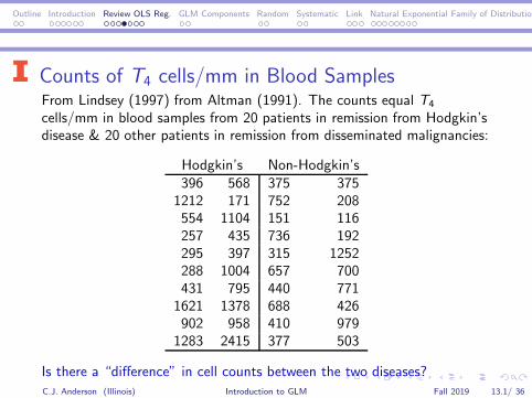
Counts of T4 cells/mm in Blood SamplesFrom Lindsey (1997) from Altman (1991). The counts equal T4

cells/mm in blood samples from 20 patients in remission from Hodgkin’sdisease & 20 other patients in remission from disseminated malignancies:

Hodgkin’s Non-Hodgkin’s396 568 375 375

1212 171 752 208554 1104 151 116257 435 736 192295 397 315 1252288 1004 657 700431 795 440 771

1621 1378 688 426902 958 410 979

1283 2415 377 503

Is there a “difference” in cell counts between the two diseases?C.J. Anderson (Illinois) Introduction to GLM Fall 2019 13.1/ 36


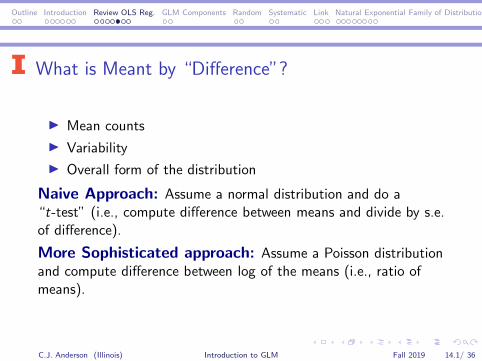
What is Meant by “Difference”?

◮ Mean counts

◮ Variability

◮ Overall form of the distribution

Naive Approach: Assume a normal distribution and do a“t-test” (i.e., compute difference between means and divide by s.e.of difference).

More Sophisticated approach: Assume a Poisson distributionand compute difference between log of the means (i.e., ratio ofmeans).



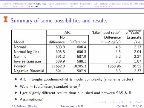
Summary of some possibilities and results

AIC “Likelihood ratio”√“Wald”

No Difference EstimateModel difference Difference in −2 log(L) /s.e.Normal 608.8 606.4 4.5 2.17Normal log link 608.8 606.3 4.5 2.04Gamma 591.2 587.9 5.2 2.27Inverse Gaussian 589.9 588.1 3.8 1.87Poisson 11652.0 10285.3 1368.96 36.52Negative Binomial 591.1 587.9 5.3 2.37

◮ AIC = weighs goodness-of-fit & model complexity (smaller is better)

◮ Wald = ( ̂parameter/ ̂standard error)2.

◮ I get slightly different results than published and between SAS & R.

◮ Assumptions?



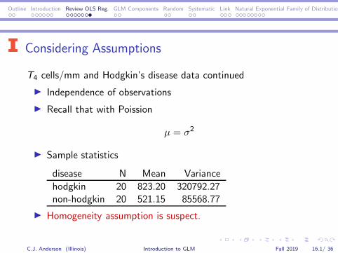
Considering Assumptions

T4 cells/mm and Hodgkin’s disease data continued

◮ Independence of observations

◮ Recall that with Poission

µ = σ2

◮ Sample statistics

disease N Mean Variance

hodgkin 20 823.20 320792.27non-hodgkin 20 521.15 85568.77

◮ Homogeneity assumption is suspect.



Components of Generalized Linear Models

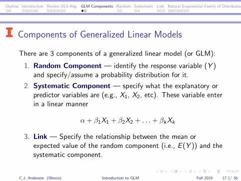
There are 3 components of a generalized linear model (or GLM):

1. Random Component — identify the response variable (Y )and specify/assume a probability distribution for it.

2. Systematic Component — specify what the explanatory orpredictor variables are (e.g., X1, X2, etc). These variable enterin a linear manner

α+ β1X1 + β2X2 + . . .+ βkXk

3. Link — Specify the relationship between the mean orexpected value of the random component (i.e., E (Y )) and thesystematic component.



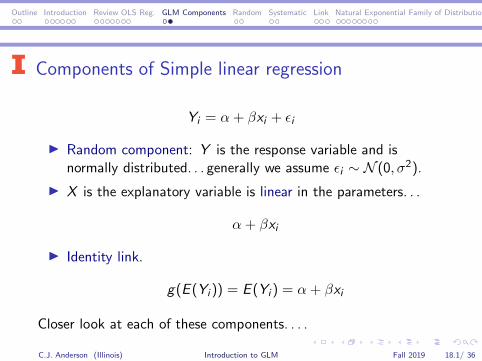
Components of Simple linear regression

Yi = α+ βxi + ǫi

◮ Random component: Y is the response variable and isnormally distributed. . . generally we assume ǫi ∼ N (0, σ2).

◮ X is the explanatory variable is linear in the parameters. . .

α+ βxi

◮ Identity link.

g(E (Yi )) = E (Yi ) = α+ βxi

Closer look at each of these components. . . .



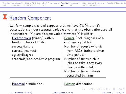
Random Component

Let N = sample size and suppose that we have Y1,Y2, . . . ,YN

observations on our response variable and that the observations are allindependent. Y ’s are discrete variables where Y is either

Dichotomous (binary) with a Counts (including cells of afixed numbers of trials. contingency table):success/failure Number of people who diecorrect/incorrect from AIDS during a givenagree/disagree time period.academic/non-academic program Number of times a child

tries to take a toy awayfrom another child.

Number of times patentsgenerated by firms.

Binomial distribution. Poisson distribution



Distributions for Discrete Variables

Thus the two distributions we will be primarily using are

◮ Binomial

◮ Poisson

With GLMs, you can use any distribution that belongs to the“exponential family of distributions”. This is a wide class ofdistributions that have many of the “nice”properties of the Normaldistribution. (we’ll look at this in a bit more detail later).



Systematic Component

As in ordinary regression, we will be modelling means. The focus ison the expected value of our response variable

E (Y ) = µ

We want to investigate whether and how µ varies as a function ofthe levels of our predictor or explanatory variables, X ’s.

The systematic component of the model consists of a set ofexplanatory variables and some linear function of them.

βo + β1x1 + β2x2 + β3x3 + . . .+ βkxk .

This linear combination of our explanatory variables is referred toas a “linear predictor”.



Linear Predictor

This restriction to a linear predictor is not all that restrictive.

For example,

◮ x3 = x1x2 — an “interaction”.

◮ x1 ⇒ x21 — a “curvilinear” relationship.

◮ x2 ⇒ log(x2) — a “curvilinear” relationship.

βo + β1x21 + β2 log(x2) + β3x

21 log(x2)

This part of the model is very much like what you know withrespect to ordinary linear regression.



The Link Function

“Left hand” side of an “Right hand” side of theequation/model — the equation— the systematicrandom component, component; that is,

E (Y ) = µ α+ β1x1 + β2x2 + . . .+ βkxk

We now need to “link” the two sides.

How is µ = E (Y ) related to α+ β1x1 + β2x2 + . . .+ βkxk?

We do this using a “Link Function” =⇒ g(µ)

g(µ) = α+ β1x1 + β2x2 + . . .+ βkxk



More about the Link Function◮ Important things about g(.):

◮ This function g(.) is “monotone” — as the systematic part getslarger, µ gets larger (or smaller).

◮ The relationship between E (Y ) and the systematic part can benon-linear.

◮ Some common links are◮ Identity (ordinary regression, ANOVA, ANCOVA):

E (Y ) = α+ βx

◮ Log link which is often used when Y is nonnegative (i.e.,0 ≤ Y )

log(E (Y )) = log(µ) = α+ βx

This yields a “loglinear” model.◮ Logit link, which is often used when 0 ≤ µ ≤ 1 (when response

is dictohomous/binary and we’re interested in a probability).

log(µ/(1− µ)) = α+ βx



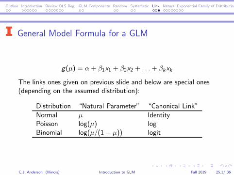
General Model Formula for a GLM

g(µ) = α+ β1x1 + β2x2 + . . .+ βkxk

The links ones given on previous slide and below are special ones(depending on the assumed distribution):

Distribution “Natural Parameter” “Canonical Link”

Normal µ IdentityPoisson log(µ) logBinomial log(µ/(1 − µ)) logit



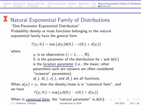
Natural Exponential Family of Distributions“One-Parameter Exponential Distribution”

Probability density or mass functions belonging to the naturalexponential family have the general form

f (yi ; θi) = exp {a(yi)b(θi )− c(θi ) + d(yi )}where

yi is an observation (i = 1, . . . ,N).θi is the parameter of the distribution for i and b(θi )is the location parameter (i.e., the mean; otherparameters such are variance are often considered“nuisance” parameters).a(.), b(.), c(.), and d(.) are all functions.

When a(yi) = yi , then the density/mass is in “canonical form”, andwe have

f (yi ; θi ) = exp{yib(θi )− c(θi ) + d(yi )}When in canonical form, the “natural parameter” is b(θi ).C.J. Anderson (Illinois) Introduction to GLM Fall 2019 26.1/ 36


According to Webester’s Dictionary

Canonical means

◮ conforming to a general rule

◮ reduced to the simplest or clearest scheme possible

◮ the simplest form of a matrix (specifically the form of a squarematrix that has zero off-diagonals).

Now for some examples. . .



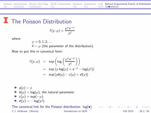
The Poisson Distribution

f (y ;µ) =µye−µ

y !

wherey = 0, 1, 2, . . .θ = µ (the parameter of the distribution).

Now to put this in canonical form:

f (y ;µ) = exp

(

log

(

µye−µ

y !

))

= exp(

y log(µ) + e−µ − log(y !))

= exp (yb(µ)− c(µ) + d(y))

◮ a(y) = y◮ b(µ) = log(µ), the natural parameter.◮ c(µ) = exp(−µ).◮ d(y) = − log(y !).

The canonical link for the Poisson distribution: log(•).C.J. Anderson (Illinois) Introduction to GLM Fall 2019 28.1/ 36


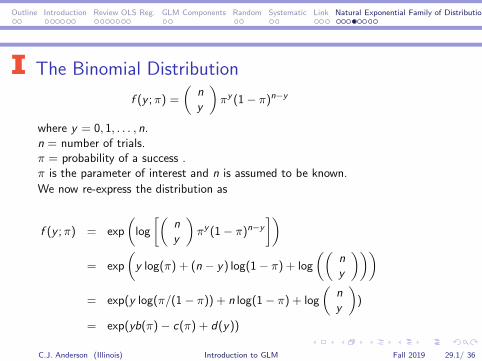
The Binomial Distribution

f (y ;π) =

(

n

y

)

πy (1− π)n−y

where y = 0, 1, . . . , n.n = number of trials.π = probability of a success .π is the parameter of interest and n is assumed to be known.

We now re-express the distribution as

f (y ;π) = exp

(

log

[(

n

y

)

πy (1− π)n−y

])

= exp

(

y log(π) + (n − y) log(1− π) + log

((

n

y

)))

= exp(y log(π/(1 − π)) + n log(1− π) + log

(

n

y

)

)

= exp(yb(π)− c(π) + d(y))



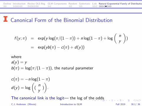
Canonical Form of the Binomial Distribution

f (y ;π) = exp(y log(π/(1 − π)) + n log(1− π) + log

(

n

y

)

)

= exp(yb(π)− c(π) + d(y))

wherea(y) = y

b(π) = log(π/(1 − π)), the natural parameter

c(π) = −n log(1− π)

d(y) = log

(

(n

y)

)

.

The canonical link is the logit— the log of the odds



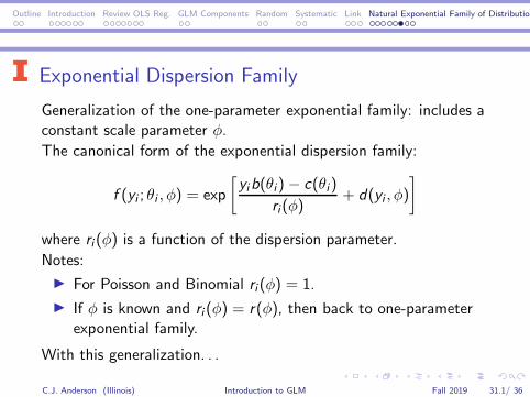
Exponential Dispersion Family

Generalization of the one-parameter exponential family: includes aconstant scale parameter φ.

The canonical form of the exponential dispersion family:

f (yi ; θi , φ) = exp

[

yib(θi)− c(θi)

ri(φ)+ d(yi , φ)

]

where ri (φ) is a function of the dispersion parameter.

Notes:

◮ For Poisson and Binomial ri (φ) = 1.

◮ If φ is known and ri (φ) = r(φ), then back to one-parameterexponential family.

With this generalization. . .



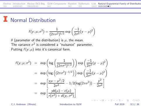
Normal Distribution

f (y ;µ;σ2) =1

(2πσ2)1/2exp

(−1

2σ2(y − µ)2

)

θ (parameter of the distribution) is µ, the mean.The variance σ2 is considered a “nuisance” parameter.

Putting f (y ;µ) into it’s canonical form.

f (y ;µ;σ2) = exp

(

log

(

1

(2πσ2)1/2

))

exp

( −1

2σ2(y − µ)2

)

= exp(

log(

(2πσ2)−1/2))

exp

( −1

2σ2(y − µ)2

)

= exp

[

yµ− µ2/2

2σ2− 1/2(log(2πσ2))− y2

2σ2

]

= exp

[

yb(µ)− c(µ)

r(σ2) + d(yi , σ2)

]



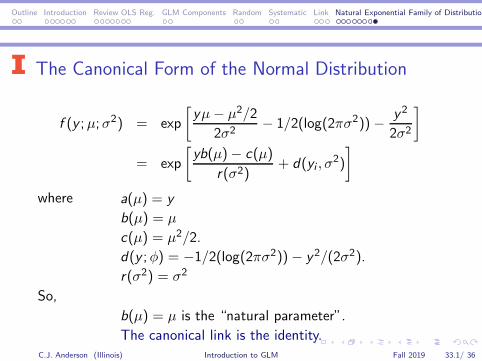
The Canonical Form of the Normal Distribution

f (y ;µ;σ2) = exp

[

yµ− µ2/2

2σ2− 1/2(log(2πσ2))− y2

2σ2

]

= exp

[

yb(µ)− c(µ)

r(σ2)+ d(yi , σ

2)

]

where a(µ) = y

b(µ) = µ

c(µ) = µ2/2.

d(y ;φ) = −1/2(log(2πσ2))− y2/(2σ2).

r(σ2) = σ2

So,

b(µ) = µ is the “natural parameter”.

The canonical link is the identity.C.J. Anderson (Illinois) Introduction to GLM Fall 2019 33.1/ 36


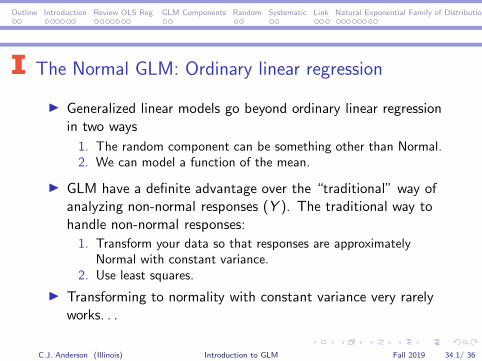
The Normal GLM: Ordinary linear regression

◮ Generalized linear models go beyond ordinary linear regressionin two ways

1. The random component can be something other than Normal.2. We can model a function of the mean.

◮ GLM have a definite advantage over the “traditional” way ofanalyzing non-normal responses (Y ). The traditional way tohandle non-normal responses:

1. Transform your data so that responses are approximatelyNormal with constant variance.

2. Use least squares.

◮ Transforming to normality with constant variance very rarelyworks. . .



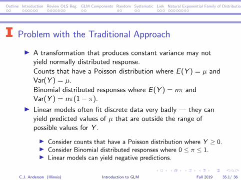
Problem with the Traditional Approach

◮ A transformation that produces constant variance may notyield normally distributed response.

Counts that have a Poisson distribution where E (Y ) = µ andVar(Y ) = µ.

Binomial distributed responses where E (Y ) = nπ andVar(Y ) = nπ(1− π).

◮ Linear models often fit discrete data very badly — they canyield predicted values of µ that are outside the range ofpossible values for Y .

◮ Consider counts that have a Poisson distribution where Y ≥ 0.◮ Consider Binomial distributed responses where 0 ≤ π ≤ 1.◮ Linear models can yield negative predictions.



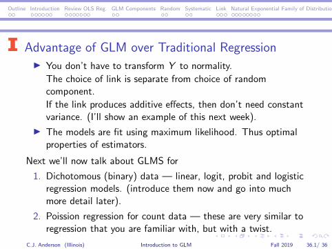
Advantage of GLM over Traditional Regression◮ You don’t have to transform Y to normality.

The choice of link is separate from choice of randomcomponent.

If the link produces additive effects, then don’t need constantvariance. (I’ll show an example of this next week).

◮ The models are fit using maximum likelihood. Thus optimalproperties of estimators.

Next we’ll now talk about GLMS for

1. Dichotomous (binary) data — linear, logit, probit and logisticregression models. (introduce them now and go into muchmore detail later).

2. Poission regression for count data — these are very similar toregression that you are familiar with, but with a twist.


Introduction to Generalized Linear Models - Edps/Psych/Soc 589€¦ · Components of Generalized...

Documents

Transcript of Introduction to Generalized Linear Models - Edps/Psych/Soc 589€¦ · Components of Generalized...