Introduction to General and Generalized Linear Models ...hmad/GLM/slides/lect13.pdf · Introduction...
35
Introduction to General and Generalized Linear Models Hierarchical models Henrik Madsen Poul Thyregod Informatics and Mathematical Modelling Technical University of Denmark DK-2800 Kgs. Lyngby January 2011 Henrik Madsen Poul Thyregod (IMM-DTU) Chapman & Hall January 2011 1 / 35
Transcript of Introduction to General and Generalized Linear Models ...hmad/GLM/slides/lect13.pdf · Introduction...
Introduction to General and Generalized Linear Models
Hierarchical models
Henrik MadsenPoul Thyregod
Informatics and Mathematical ModellingTechnical University of Denmark
DK-2800 Kgs. Lyngby
January 2011
Henrik Madsen Poul Thyregod (IMM-DTU) Chapman & Hall January 2011 1 / 35
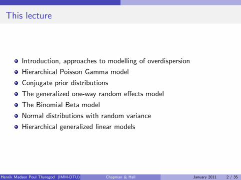
This lecture
Introduction, approaches to modelling of overdispersion
Hierarchical Poisson Gamma model
Conjugate prior distributions
The generalized one-way random effects model
The Binomial Beta model
Normal distributions with random variance
Hierarchical generalized linear models
Henrik Madsen Poul Thyregod (IMM-DTU) Chapman & Hall January 2011 2 / 35
Introduction, approaches to modelling of overdispersion
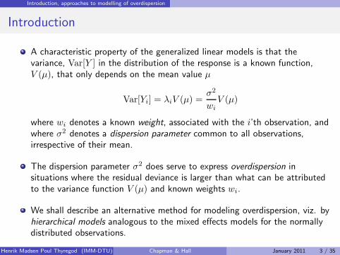
Introduction
A characteristic property of the generalized linear models is that thevariance, Var[Y ] in the distribution of the response is a known function,V (µ), that only depends on the mean value µ
Var[Yi] = λiV (µ) =σ2
wi
V (µ)
where wi denotes a known weight, associated with the i’th observation, andwhere σ2 denotes a dispersion parameter common to all observations,irrespective of their mean.
The dispersion parameter σ2 does serve to express overdispersion insituations where the residual deviance is larger than what can be attributedto the variance function V (µ) and known weights wi.
We shall describe an alternative method for modeling overdispersion, viz. byhierarchical models analogous to the mixed effects models for the normallydistributed observations.
Henrik Madsen Poul Thyregod (IMM-DTU) Chapman & Hall January 2011 3 / 35
Introduction, approaches to modelling of overdispersion
Introduction
A starting point in a hierarchical modeling is an assumption that thedistribution of the random “noise” may be modeled by an exponentialdispersion family (Binomial, Poisson, etc.), and then it is a matter ofchoosing a suitable (prior) distribution of the mean-value parameterµ.
It seems natural to choose a distribution with a support that coincideswith the mean value space M rather than using a normal distribution(with a support constituting all of the real axis R).
In some applications an approach with a normal distribution of thecanonical parameter is used. Such an approach is sometimes calledgeneralized linear mixed models (GLMMs)
Henrik Madsen Poul Thyregod (IMM-DTU) Chapman & Hall January 2011 4 / 35
Introduction, approaches to modelling of overdispersion
Introduction
Although such an approach is consistent with a formal requirement ofequivalence between mean values space and support for the distribution of µin the binomial and the Poisson distribution case, the resulting marginaldistribution of the observation is seldom tractable, and the likelihood of sucha model will involve an integral which cannot in general be computedexplicitly.
Also, the canonical parameter does not have a simple physical interpretationand, therefore, an additive “true value” + error, with a normally distributed“error” on the canonical parameter to describe variation between subgroups,is not very transparent.
Instead, we shall describe an approach based on the so-called standardconjugated distribution for the mean parameter of the within groupdistribution for exponential families.
These distributions combine with the exponential families in a simple way,and lead to marginal distributions that may be expressed in a closed formsuited for likelihood calculations.
Henrik Madsen Poul Thyregod (IMM-DTU) Chapman & Hall January 2011 5 / 35
Hierarchical Poisson Gamma model
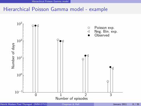
Hierarchical Poisson Gamma model - example
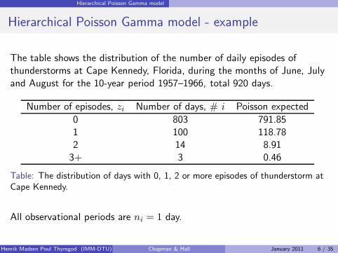
The table shows the distribution of the number of daily episodes ofthunderstorms at Cape Kennedy, Florida, during the months of June, Julyand August for the 10-year period 1957–1966, total 920 days.
Number of episodes, zi Number of days, # i Poisson expected
0 803 791.851 100 118.782 14 8.913+ 3 0.46
Table: The distribution of days with 0, 1, 2 or more episodes of thunderstorm atCape Kennedy.
All observational periods are ni = 1 day.
Henrik Madsen Poul Thyregod (IMM-DTU) Chapman & Hall January 2011 6 / 35
Hierarchical Poisson Gamma model
Hierarchical Poisson Gamma model - example
The data represents counts of events (episodes of thunderstorms)distributed in time.
A completely random distribution of the events would result in aPoisson distribution of the number of daily events.
The variance function for the Poisson distribution is V (µ) = µ;therefore, a Poisson distribution of the daily number of events wouldresult in the variance in the distribution of the daily number of eventsbeing equal to the mean, µ = y+ = 0.15 thunderstorms per day.
The empirical variance is s2 = 0.1769, which is somewhat larger thanthe average. We further note that the observed distribution hasheavier tails than the Poisson distribution. Thus, one might besuspicious of overdispersion.
Henrik Madsen Poul Thyregod (IMM-DTU) Chapman & Hall January 2011 7 / 35
Hierarchical Poisson Gamma model
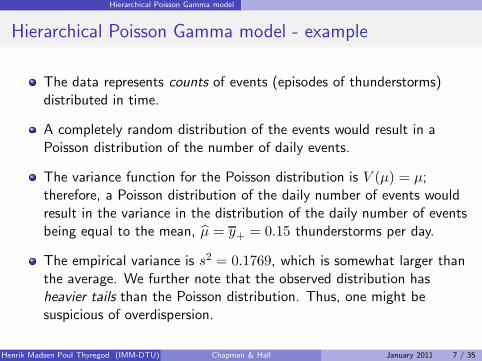
Hierarchical Poisson Gamma model - exampleNumber
ofdays
Number of episodes
Poisson exp.Neg. Bin. exp.Observed
0 1 2 3
103
102
101
100
10−1
Henrik Madsen Poul Thyregod (IMM-DTU) Chapman & Hall January 2011 8 / 35
Hierarchical Poisson Gamma model
Formulation of hierarchical model
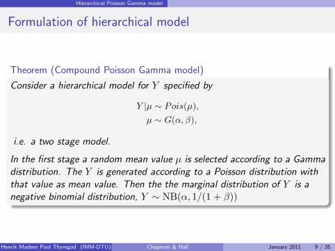
Theorem (Compound Poisson Gamma model)
Consider a hierarchical model for Y specified by
Y |µ ∼ Pois(µ),
µ ∼ G(α, β),
i.e. a two stage model.
In the first stage a random mean value µ is selected according to a Gammadistribution. The Y is generated according to a Poisson distribution withthat value as mean value. Then the the marginal distribution of Y is anegative binomial distribution, Y ∼ NB(α, 1/(1 + β))
Henrik Madsen Poul Thyregod (IMM-DTU) Chapman & Hall January 2011 9 / 35
Hierarchical Poisson Gamma model
Formulation of hierarchical model
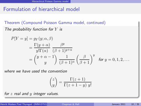
Theorem (Compound Poisson Gamma model, continued)
The probability function for Y is
P [Y = y] = gY (y;α, β)
=Γ(y + α)
y!Γ(α)
βy
(β + 1)y+α
=
(y + α− 1
y
)1
(β + 1)α
(β
β + 1
)y
for y = 0, 1, 2, . . .
where we have used the convention(z
y
)=
Γ(z + 1)
Γ(z + 1− y) y!
for z real and y integer values.
Henrik Madsen Poul Thyregod (IMM-DTU) Chapman & Hall January 2011 10 / 35
Hierarchical Poisson Gamma model
Formulation of hierarchical model
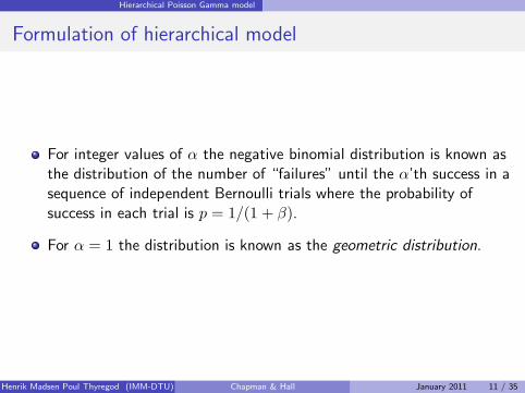
For integer values of α the negative binomial distribution is known asthe distribution of the number of “failures” until the α’th success in asequence of independent Bernoulli trials where the probability ofsuccess in each trial is p = 1/(1 + β).
For α = 1 the distribution is known as the geometric distribution.
Henrik Madsen Poul Thyregod (IMM-DTU) Chapman & Hall January 2011 11 / 35
Hierarchical Poisson Gamma model
Formulation of hierarchical model
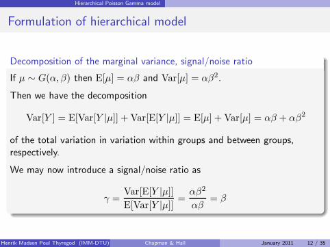
Decomposition of the marginal variance, signal/noise ratio
If µ ∼ G(α, β) then E[µ] = αβ and Var[µ] = αβ2.
Then we have the decomposition
Var[Y ] = E[Var[Y |µ]] + Var[E[Y |µ]] = E[µ] + Var[µ] = αβ + αβ2
of the total variation in variation within groups and between groups,respectively.
We may now introduce a signal/noise ratio as
γ =Var[E[Y |µ]]
E[Var[Y |µ]]=αβ2
αβ= β
Henrik Madsen Poul Thyregod (IMM-DTU) Chapman & Hall January 2011 12 / 35
Hierarchical Poisson Gamma model
Inference on individual group means
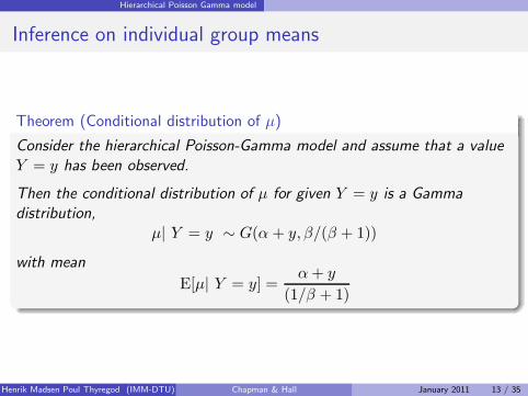
Theorem (Conditional distribution of µ)
Consider the hierarchical Poisson-Gamma model and assume that a valueY = y has been observed.
Then the conditional distribution of µ for given Y = y is a Gammadistribution,
µ| Y = y ∼ G(α + y, β/(β + 1))
with mean
E[µ| Y = y] =α+ y
(1/β + 1)
Henrik Madsen Poul Thyregod (IMM-DTU) Chapman & Hall January 2011 13 / 35
Hierarchical Poisson Gamma model
Inference on individual group means
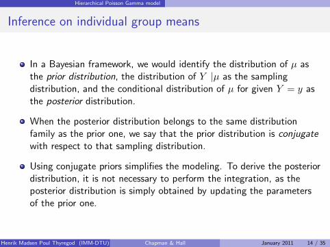
In a Bayesian framework, we would identify the distribution of µ asthe prior distribution, the distribution of Y |µ as the samplingdistribution, and the conditional distribution of µ for given Y = y asthe posterior distribution.
When the posterior distribution belongs to the same distributionfamily as the prior one, we say that the prior distribution is conjugatewith respect to that sampling distribution.
Using conjugate priors simplifies the modeling. To derive the posteriordistribution, it is not necessary to perform the integration, as theposterior distribution is simply obtained by updating the parametersof the prior one.
Henrik Madsen Poul Thyregod (IMM-DTU) Chapman & Hall January 2011 14 / 35
Hierarchical Poisson Gamma model
Inference on individual group means
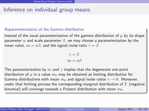
Reparameterization of the Gamma distribution
Instead of the usual parameterization of the gamma distribution of µ by its shapeparameter α and scale parameter β, we may choose a parameterization by themean value, m = αβ, and the signal/noise ratio γ = β
γ = β
m = αβ
The parameterization by m and γ implies that the degenerate one-pointdistribution of µ in a value m0 may be obtained as limiting distribution forGamma distributions with mean m0 and signal/noise ratios γ → 0. Moreover,under that limiting process the corresponding marginal distribution of Y (negativebinomial) will converge towards a Poisson distribution with mean m0.
Henrik Madsen Poul Thyregod (IMM-DTU) Chapman & Hall January 2011 15 / 35
Conjugate prior distributions
Conjugate prior distributions
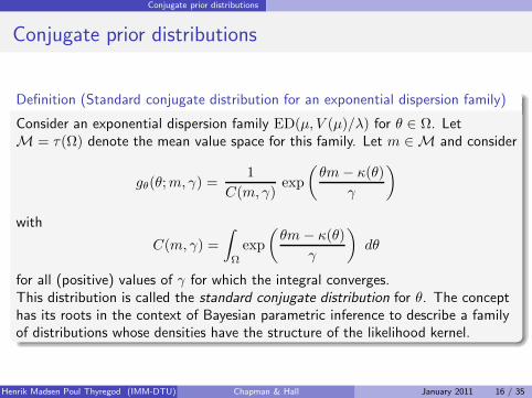
Definition (Standard conjugate distribution for an exponential dispersion family)
Consider an exponential dispersion family ED(µ, V (µ)/λ) for θ ∈ Ω. LetM = τ(Ω) denote the mean value space for this family. Let m ∈ M and consider
gθ(θ;m, γ) =1
C(m, γ)exp
(θm− κ(θ)
γ
)
with
C(m, γ) =
∫
Ω
exp
(θm− κ(θ)
γ
)dθ
for all (positive) values of γ for which the integral converges.This distribution is called the standard conjugate distribution for θ. The concepthas its roots in the context of Bayesian parametric inference to describe a familyof distributions whose densities have the structure of the likelihood kernel.
Henrik Madsen Poul Thyregod (IMM-DTU) Chapman & Hall January 2011 16 / 35
Conjugate prior distributions
Conjugate prior distributions
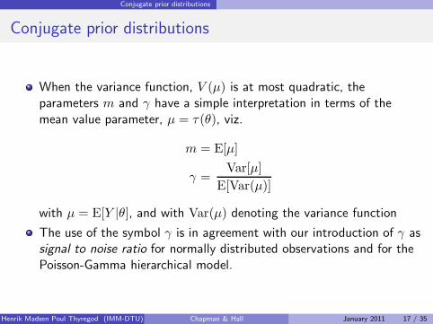
When the variance function, V (µ) is at most quadratic, theparameters m and γ have a simple interpretation in terms of themean value parameter, µ = τ(θ), viz.
m = E[µ]
γ =Var[µ]
E[Var(µ)]
with µ = E[Y |θ], and with Var(µ) denoting the variance function
The use of the symbol γ is in agreement with our introduction of γ assignal to noise ratio for normally distributed observations and for thePoisson-Gamma hierarchical model.
Henrik Madsen Poul Thyregod (IMM-DTU) Chapman & Hall January 2011 17 / 35
Conjugate prior distributions
Conjugate prior distributions
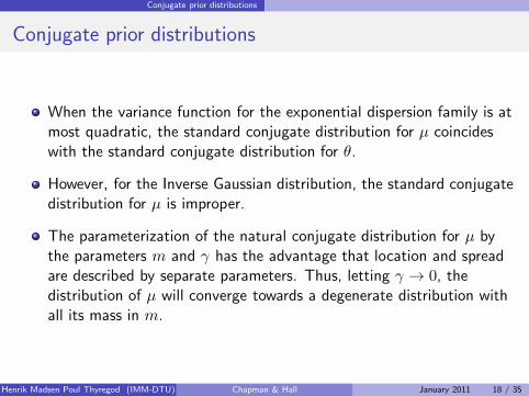
When the variance function for the exponential dispersion family is atmost quadratic, the standard conjugate distribution for µ coincideswith the standard conjugate distribution for θ.
However, for the Inverse Gaussian distribution, the standard conjugatedistribution for µ is improper.
The parameterization of the natural conjugate distribution for µ bythe parameters m and γ has the advantage that location and spreadare described by separate parameters. Thus, letting γ → 0, thedistribution of µ will converge towards a degenerate distribution withall its mass in m.
Henrik Madsen Poul Thyregod (IMM-DTU) Chapman & Hall January 2011 18 / 35
The generalized one-way random effects model
The generalized one-way random effects model
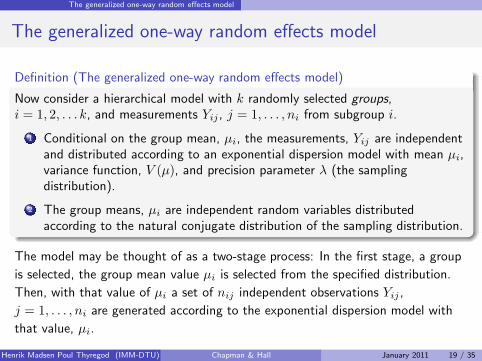
Definition (The generalized one-way random effects model)
Now consider a hierarchical model with k randomly selected groups,i = 1, 2, . . . k, and measurements Yij , j = 1, . . . , ni from subgroup i.
1 Conditional on the group mean, µi, the measurements, Yij are independentand distributed according to an exponential dispersion model with mean µi,variance function, V (µ), and precision parameter λ (the samplingdistribution).
2 The group means, µi are independent random variables distributedaccording to the natural conjugate distribution of the sampling distribution.
The model may be thought of as a two-stage process: In the first stage, a group
is selected, the group mean value µi is selected from the specified distribution.
Then, with that value of µi a set of nij independent observations Yij ,
j = 1, . . . , ni are generated according to the exponential dispersion model with
that value, µi.
Henrik Madsen Poul Thyregod (IMM-DTU) Chapman & Hall January 2011 19 / 35
The generalized one-way random effects model
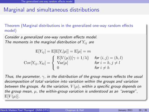
Marginal and simultaneous distributions
Theorem (Marginal distributions in the generalized one-way random effectsmodel)
Consider a generalized one-way random effects model.The moments in the marginal distribution of Yij are
E[Yij ] = E[E[Yi|µ]] = E[µ] = m
Cov[Yij , Yhl] =
E[V (µ)]γ + 1/λ for (i, j) = (h, l)Var[µ] for i = h, j 6= l0 for i 6= h
Thus, the parameter, γ, in the distribution of the group means reflects the usualdecomposition of total variation into variation within the groups and variationbetween the groups. As the variation, V (µ), within a specific group depends onthe group mean, µ, the within-group variation is understood as an “average”,E[V (µ)].
Henrik Madsen Poul Thyregod (IMM-DTU) Chapman & Hall January 2011 20 / 35
The generalized one-way random effects model
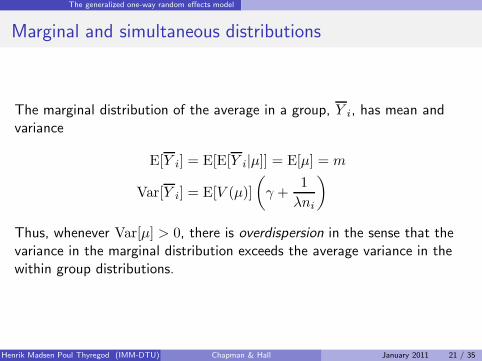
Marginal and simultaneous distributions
The marginal distribution of the average in a group, Y i, has mean andvariance
E[Y i] = E[E[Y i|µ]] = E[µ] = m
Var[Y i] = E[V (µ)]
(γ +
1
λni
)
Thus, whenever Var[µ] > 0, there is overdispersion in the sense that thevariance in the marginal distribution exceeds the average variance in thewithin group distributions.
Henrik Madsen Poul Thyregod (IMM-DTU) Chapman & Hall January 2011 21 / 35
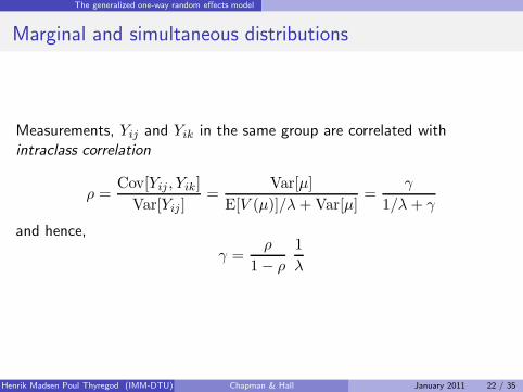
The generalized one-way random effects model
Marginal and simultaneous distributions
Measurements, Yij and Yik in the same group are correlated withintraclass correlation
ρ =Cov[Yij , Yik]
Var[Yij ]=
Var[µ]
E[V (µ)]/λ+Var[µ]=
γ
1/λ+ γ
and hence,
γ =ρ
1− ρ
1
λ
Henrik Madsen Poul Thyregod (IMM-DTU) Chapman & Hall January 2011 22 / 35
The generalized one-way random effects model
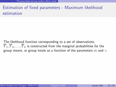
Estimation of fixed parameters - Maximum likelihood
estimation
The likelihood function corresponding to a set of observations,Y 1, Y 2, . . . , Y k is constructed from the marginal probabilities for thegroup means, or group totals as a function of the parameters m and γ.
Henrik Madsen Poul Thyregod (IMM-DTU) Chapman & Hall January 2011 23 / 35
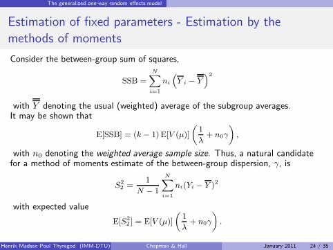
The generalized one-way random effects model
Estimation of fixed parameters - Estimation by the
methods of moments
Consider the between-group sum of squares,
SSB =N∑
i=1
ni
(
Y i − Y)
2
with Y denoting the usual (weighted) average of the subgroup averages.It may be shown that
E[SSB] = (k − 1) E[V (µ)]
(
1
λ+ n0γ
)
,
with n0 denoting the weighted average sample size. Thus, a natural candidatefor a method of moments estimate of the between-group dispersion, γ, is
S2
2 =1
N − 1
N∑
i=1
ni(Yi − Y )2
with expected value
E[S2
2 ] = E[V (µ)]
(
1
λ+ n0γ
)
.
Henrik Madsen Poul Thyregod (IMM-DTU) Chapman & Hall January 2011 24 / 35
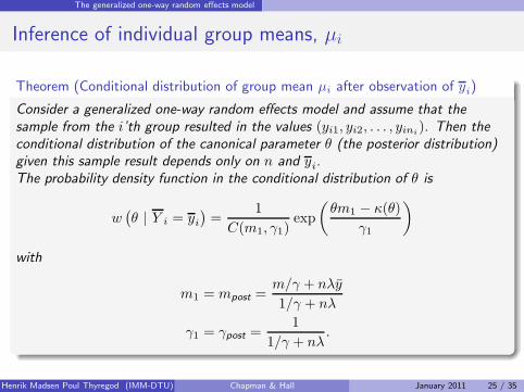
The generalized one-way random effects model
Inference of individual group means, µi
Theorem (Conditional distribution of group mean µi after observation of yi)
Consider a generalized one-way random effects model and assume that thesample from the i’th group resulted in the values (yi1, yi2, . . . , yini
). Then theconditional distribution of the canonical parameter θ (the posterior distribution)given this sample result depends only on n and yi.The probability density function in the conditional distribution of θ is
w(θ | Y i = yi
)=
1
C(m1, γ1)exp
(θm1 − κ(θ)
γ1
)
with
m1 = mpost =m/γ + nλy
1/γ + nλ
γ1 = γpost =1
1/γ + nλ.
Henrik Madsen Poul Thyregod (IMM-DTU) Chapman & Hall January 2011 25 / 35
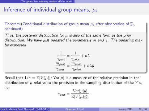
The generalized one-way random effects model
Inference of individual group means, µi
Theorem (Conditional distribution of group mean µi after observation of yi,continued)
Thus, the posterior distribution for µ is also of the same form as the priordistribution. We have just updated the parameters m and γ. The updating maybe expressed
1
γpost=
1
γprior+ nλ
mpost
γpost=mpriori
γpriori+ nλy
Recall that 1/γ = E[V (µ)]/Var[µ] is a measure of the relative precision in thedistribution of µ relative to the precision in the sampling distribution of the Y ’s,i.e.
γpost =Var[µ|y]
E[V (µ)|y].
Henrik Madsen Poul Thyregod (IMM-DTU) Chapman & Hall January 2011 26 / 35
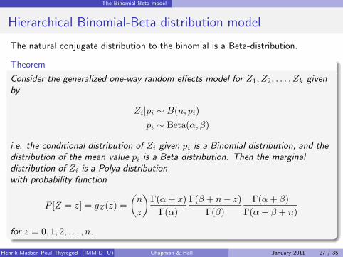
The Binomial Beta model
Hierarchical Binomial-Beta distribution model
The natural conjugate distribution to the binomial is a Beta-distribution.
Theorem
Consider the generalized one-way random effects model for Z1, Z2, . . . , Zk givenby
Zi|pi ∼ B(n, pi)
pi ∼ Beta(α, β)
i.e. the conditional distribution of Zi given pi is a Binomial distribution, and thedistribution of the mean value pi is a Beta distribution. Then the marginaldistribution of Zi is a Polya distributionwith probability function
P [Z = z] = gZ(z) =
(n
z
)Γ(α+ x)
Γ(α)
Γ(β + n− z)
Γ(β)
Γ(α+ β)
Γ(α + β + n)
for z = 0, 1, 2, . . . , n.
Henrik Madsen Poul Thyregod (IMM-DTU) Chapman & Hall January 2011 27 / 35
The Binomial Beta model
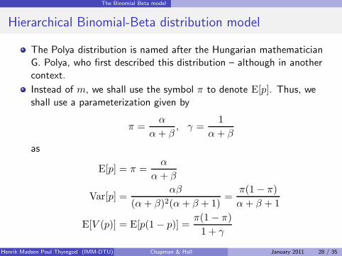
Hierarchical Binomial-Beta distribution model
The Polya distribution is named after the Hungarian mathematicianG. Polya, who first described this distribution – although in anothercontext.
Instead of m, we shall use the symbol π to denote E[p]. Thus, weshall use a parameterization given by
π =α
α+ β, γ =
1
α+ β
as
E[p] = π =α
α+ β
Var[p] =αβ
(α+ β)2(α+ β + 1)=
π(1− π)
α+ β + 1
E[V (p)] = E[p(1− p)] =π(1− π)
1 + γ
Henrik Madsen Poul Thyregod (IMM-DTU) Chapman & Hall January 2011 28 / 35
The Binomial Beta model
Hierarchical Binomial-Beta distribution model
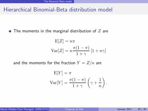
The moments in the marginal distribution of Z are
E[Z] = nπ
Var[Z] = nπ(1− π)
1 + γ[1 + nγ]
and the moments for the fraction Y = Z/n are
E[Y ] = π
Var[Y ] =π(1− π)
1 + γ
(γ +
1
n
).
Henrik Madsen Poul Thyregod (IMM-DTU) Chapman & Hall January 2011 29 / 35
The Binomial Beta model
Estimation of individual group means
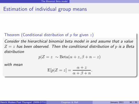
Theorem (Conditional distribution of p for given z)
Consider the hierarchical binomial beta model in and assume that a valueZ = z has been observed. Then the conditional distribution of p is a Betadistribution
p|Z = z ∼ Beta(α+ z, β + n− z)
with mean
E[p|Z = z] =α+ z
α+ β + n.
Henrik Madsen Poul Thyregod (IMM-DTU) Chapman & Hall January 2011 30 / 35
The Binomial Beta model
Estimation of individual group means
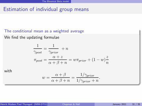
The conditional mean as a weighted average
We find the updating formulae
1
γpost=
1
γprior+ n
πpost =α+ z
α+ β + n= wπprior + (1− w)
z
n
with
w =α+ β
α+ β + n=
1/γprior1/γprior + n
.
Henrik Madsen Poul Thyregod (IMM-DTU) Chapman & Hall January 2011 31 / 35
Normal distributions with random variance
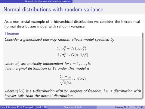
Normal distributions with random variance
As a non-trivial example of a hierarchical distribution we consider the hierarchicalnormal distribution model with random variance:
Theorem
Consider a generalized one-way random effects model specified by
Yi|σ2
i ∼ N(µ, σ2
i )
1/σ2
i ∼ G(α, 1/β)
where σ2i are mutually independent for i = 1, . . . , k.
The marginal distribution of Yi under this model is
Yi − µ√β/α
∼ t(2α)
where t(2α) is a t-distribution with 2α degrees of freedom, i.e. a distribution withheavier tails than the normal distribution.
Henrik Madsen Poul Thyregod (IMM-DTU) Chapman & Hall January 2011 32 / 35
Hierarchical generalized linear models
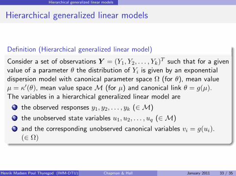
Hierarchical generalized linear models
Definition (Hierarchical generalized linear model)
Consider a set of observations Y = (Y1, Y2, . . . , Yk)T such that for a given
value of a parameter θ the distribution of Yi is given by an exponentialdispersion model with canonical parameter space Ω (for θ), mean valueµ = κ′(θ), mean value space M (for µ) and canonical link θ = g(µ).The variables in a hierarchical generalized linear model are
1 the observed responses y1, y2, . . . , yk (∈ M)
2 the unobserved state variables u1, u2, . . . , uq (∈ M)
3 and the corresponding unobserved canonical variables vi = g(ui).(∈ Ω)
Henrik Madsen Poul Thyregod (IMM-DTU) Chapman & Hall January 2011 33 / 35
Hierarchical generalized linear models
Hierarchical generalized linear models
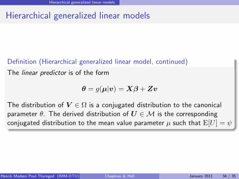
Definition (Hierarchical generalized linear model, continued)
The linear predictor is of the form
θ = g(µ|v) = Xβ +Zv
The distribution of V ∈ Ω is a conjugated distribution to the canonicalparameter θ. The derived distribution of U ∈ M is the correspondingconjugated distribution to the mean value parameter µ such that E[U ] = ψ
Henrik Madsen Poul Thyregod (IMM-DTU) Chapman & Hall January 2011 34 / 35
Hierarchical generalized linear models
Hierarchical generalized linear models
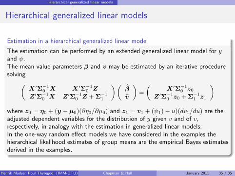
Estimation in a hierarchical generalized linear model
The estimation can be performed by an extended generalized linear model for yand ψ.The mean value parameters β and v may be estimated by an iterative proceduresolving
(X ′
Σ−1
0X X ′
Σ−1
0Z
Z ′Σ
−1
0X Z ′
Σ−1
0Z +Σ
−1
1
)(β
v
)=
(X ′
Σ−1
0z0
Z ′Σ
−1
0z0 +Σ
−1
1z1
)
where z0 = η0 + (y − µ0)(∂η0/∂µ0) and z1 = v1 + (ψ1)− u)(dv1/du) are theadjusted dependent variables for the distribution of y given v and of v,respectively, in analogy with the estimation in generalized linear models.In the one-way random effect models we have considered in the examples thehierarchical likelihood estimates of group means are the empirical Bayes estimatesderived in the examples.
Henrik Madsen Poul Thyregod (IMM-DTU) Chapman & Hall January 2011 35 / 35