Introduction to General and Generalized Linear …hmad/GLM/slides/lect10.pdfIntroduction to General...

Introduction to General and Generalized Linear Models

Mixed effects models - Part II

Henrik MadsenPoul Thyregod

Informatics and Mathematical ModellingTechnical University of Denmark

DK-2800 Kgs. Lyngby

January 2011

Henrik Madsen Poul Thyregod (IMM-DTU) Chapman & Hall January 2011 1 / 29

This lecture

One-way random effects model, continued

More examples of hierarchical variation

General linear mixed effects models


One-way random effects model

Estimation of parameters

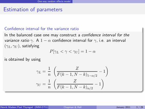
Confidence interval for the variance ratio

In the balanced case one may construct a confidence interval for thevariance ratio γ. A 1− α confidence interval for γ, i.e. an interval(γL, γU ), satisfying

P [γL < γ < γU ] = 1− α

is obtained by using

γL =1

n

(Z

F (k − 1, N − k)1−α/2− 1

)

γU =1

n

(Z

F (k − 1, N − k)α/2− 1

)




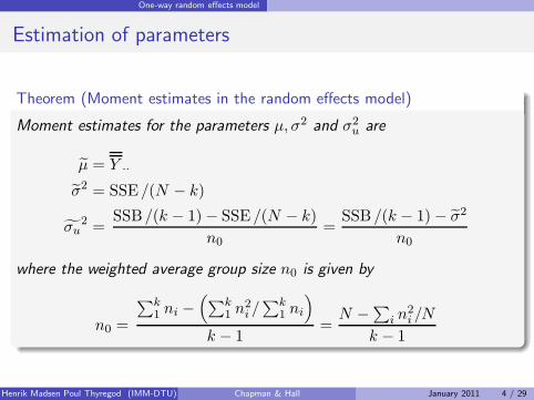
Theorem (Moment estimates in the random effects model)

Moment estimates for the parameters µ, σ2 and σ2u are

µ = Y··

σ2 = SSE /(N − k)

σu2 =

SSB/(k − 1)− SSE /(N − k)

n0

=SSB /(k − 1)− σ2

n0

where the weighted average group size n0 is given by

n0 =

∑k1ni −

(∑k1n2i /

∑k1ni

)

k − 1=

N −∑

i n2i /N

k − 1




Distribution of “residual” sum of squares

In the balanced case we have that

SSE ∼ σ2χ2(k(n− 1))

SSB ∼ {σ2/w(γ)}χ2(k − 1)

and that SSE and SSB are independent.




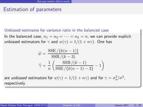
Unbiased estimates for variance ratio in the balanced case

In the balanced case, n1 = n2 = · · · = nk = n, we can provide explicitunbiased estimators for γ and w(γ) = 1/(1 + nγ). One has

w =SSE /{k(n − 1)}

SSB /(k − 3)

γ =1

n

(SSB /(k − 1)

SSE /{k(n − 1)− 2}− 1

)

are unbiased estimators for w(γ) = 1/(1 + nγ) and for γ = σ2u/σ

2,respectively.



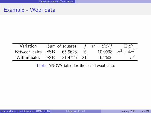
Example - Wool data

Variation Sum of squares f s2 = SS/f E[S2]

Between bales SSB 65.9628 6 10.9938 σ2 + 4σ2u

Within bales SSE 131.4726 21 6.2606 σ2

Table: ANOVA table for the baled wool data.



Example - Wool data

The test statistic for the hypothesis H0 : σ2u = 0, is

z =10.9938

6.2606= 1.76 < F0.95(6, 21) = 2.57

The p-value is P [F (6, 21) ≥ 1.76] = 0.16

Thus, the test fails to reject the hypothesis of no variation between thepurity of the bales when testing at a 5% significance level. However, asthe purpose is to describe the variation in the shipment, we will estimatethe parameters in the random effects model, irrespective of the test result.



Example - Wool data

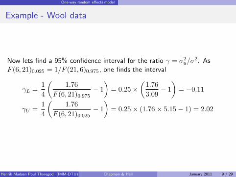
Now lets find a 95% confidence interval for the ratio γ = σ2u/σ

2. AsF (6, 21)0.025 = 1/F (21, 6)0.975 , one finds the interval

γL =1

4

(1.76

F (6, 21)0.975− 1

)= 0.25×

(1.76

3.09− 1

)= −0.11

γU =1

4

(1.76

F (6, 21)0.025− 1

)= 0.25× (1.76 × 5.15 − 1) = 2.02



Maximum likelihood estimates

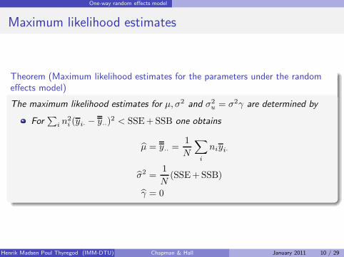
Theorem (Maximum likelihood estimates for the parameters under the randomeffects model)

The maximum likelihood estimates for µ, σ2 and σ2

u = σ2γ are determined by

For∑

i n2

i (yi· − y··)2 < SSE+SSB one obtains

µ = y··=

1

N

∑

i

niyi·

σ2 =1

N(SSE+SSB)

γ = 0




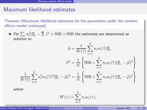
Theorem (Maximum likelihood estimates for the parameters under the randomeffects model continued)

For∑

i n2

i (yi· − y··)2 > SSE+SSB the estimates are determined as

solution to

µ =1

W (γ)

k∑

i=1

niwi(γ)yi·

σ2 =1

N

{SSE+

k∑

i=1

niwi(γ)(yi· − µ)2

}

1

W (γ)

k∑

i=1

n2

iwi(γ)2(yi· − µ)2 =

1

N

{SSE+

k∑

i=1

niwi(γ)(yi· − µ)2

}

where

W (γ) =

k∑

i=1

niwi(γ).




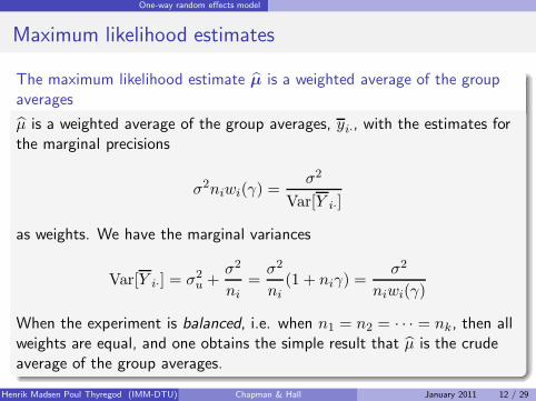
The maximum likelihood estimate µ is a weighted average of the groupaverages

µ is a weighted average of the group averages, yi·, with the estimates forthe marginal precisions

σ2niwi(γ) =σ2

Var[Y i·]

as weights. We have the marginal variances

Var[Y i·] = σ2u +

σ2

ni=

σ2

ni(1 + niγ) =

σ2

niwi(γ)

When the experiment is balanced, i.e. when n1 = n2 = · · · = nk, then allweights are equal, and one obtains the simple result that µ is the crudeaverage of the group averages.




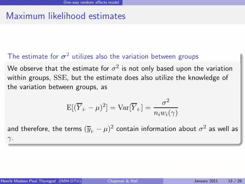
The estimate for σ2 utilizes also the variation between groups

We observe that the estimate for σ2 is not only based upon the variationwithin groups, SSE, but the estimate does also utilize the knowledge ofthe variation between groups, as

E[(Y i· − µ)2] = Var[Y i·] =σ2

niwi(γ)

and therefore, the terms (yi· − µ)2 contain information about σ2 as well asγ.




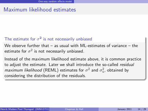
The estimate for σ2 is not necessarily unbiased

We observe further that – as usual with ML-estimates of variance – theestimate for σ2 is not necessarily unbiased.

Instead of the maximum likelihood estimate above, it is common practiceto adjust the estimate. Later we shall introduce the so-called residualmaximum likelihood (REML) estimates for σ2 and σ2

u, obtained byconsidering the distribution of the residuals.




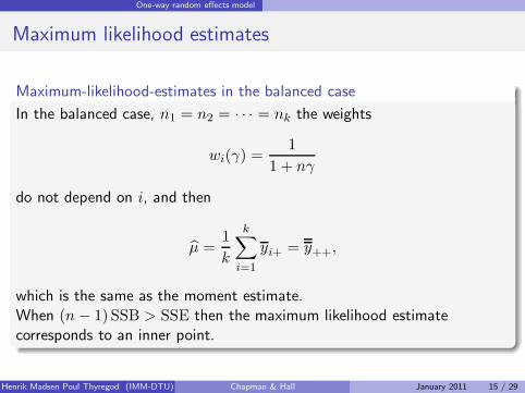
Maximum-likelihood-estimates in the balanced case

In the balanced case, n1 = n2 = · · · = nk the weights

wi(γ) =1

1 + nγ

do not depend on i, and then

µ =1

k

k∑

i=1

yi+ = y++,

which is the same as the moment estimate.When (n − 1) SSB > SSE then the maximum likelihood estimatecorresponds to an inner point.




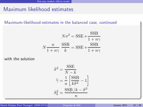
Maximum-likelihood-estimates in the balanced case, continued

Nσ2 = SSE+SSB

1 + nγ

Nn

1 + nγ

SSB

k= SSE+

SSB

1 + nγ

with the solution

σ2 =SSE

N − k

γ =1

n

[SSB

kσ2− 1

]

σ2b =

SSB /k − σ2

n



Estimation of random effects, BLUP-estimation

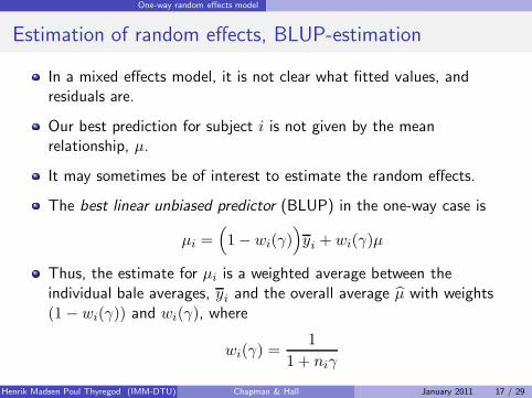
In a mixed effects model, it is not clear what fitted values, andresiduals are.

Our best prediction for subject i is not given by the meanrelationship, µ.

It may sometimes be of interest to estimate the random effects.

The best linear unbiased predictor (BLUP) in the one-way case is

µi =(1− wi(γ)

)yi + wi(γ)µ

Thus, the estimate for µi is a weighted average between theindividual bale averages, yi and the overall average µ with weights(1− wi(γ)) and wi(γ), where

wi(γ) =1

1 + niγ




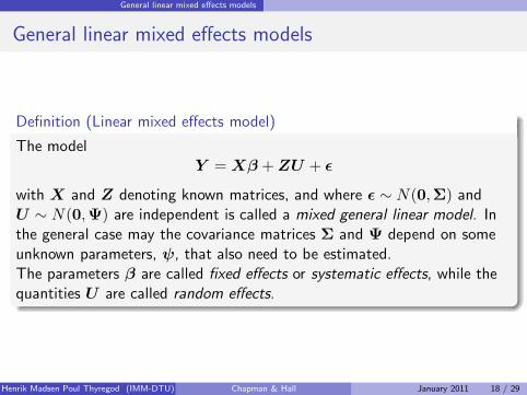
Definition (Linear mixed effects model)

The modelY =Xβ +ZU + ǫ

with X and Z denoting known matrices, and where ǫ ∼ N(0,Σ) andU ∼ N(0,Ψ) are independent is called a mixed general linear model. Inthe general case may the covariance matrices Σ and Ψ depend on someunknown parameters, ψ, that also need to be estimated.The parameters β are called fixed effects or systematic effects, while thequantities U are called random effects.




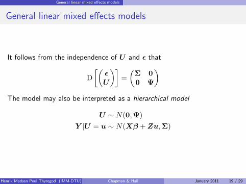
It follows from the independence of U and ǫ that

D

[(ǫ

U

)]=

(Σ 0

0 Ψ

)

The model may also be interpreted as a hierarchical model

U ∼ N(0,Ψ)

Y |U = u ∼ N(Xβ +Zu,Σ)




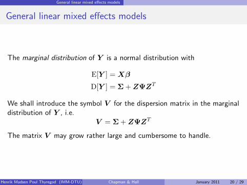
The marginal distribution of Y is a normal distribution with

E[Y ] =Xβ

D[Y ] = Σ+ZΨZT

We shall introduce the symbol V for the dispersion matrix in the marginaldistribution of Y , i.e.

V = Σ+ZΨZT

The matrix V may grow rather large and cumbersome to handle.



One-way model with random effects - example

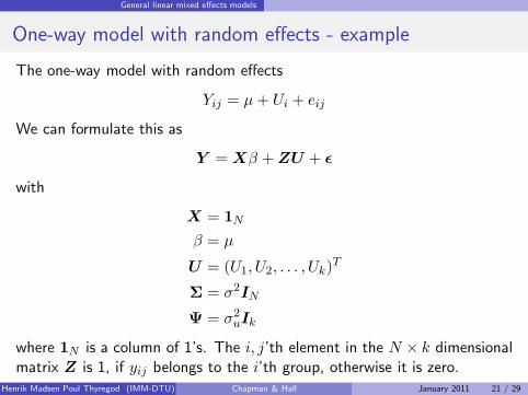
The one-way model with random effects

Yij = µ+ Ui + eij

We can formulate this as

Y =Xβ +ZU + ǫ

with

X = 1N

β = µ

U = (U1, U2, . . . , Uk)T

Σ = σ2IN

Ψ = σ2uIk

where 1N is a column of 1’s. The i, j’th element in the N × k dimensionalmatrix Z is 1, if yij belongs to the i’th group, otherwise it is zero.



Estimation of fixed effects and variance parameters

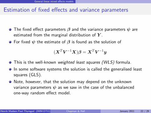
The fixed effect parameters β and the variance parameters ψ areestimated from the marginal distribution of Y .

For fixed ψ the estimate of β is found as the solution of

(XTV −1X)β =XTV −1y

This is the well-known weighted least squares (WLS) formula.

In some software systems the solution is called the generalised leastsquares (GLS).

Note, however, that the solution may depend on the unknownvariance parameters ψ as we saw in the case of the unbalancedone-way random effect model.




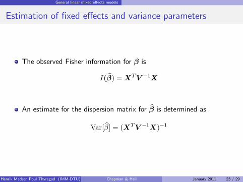
The observed Fisher information for β is

I(β) =XTV −1X

An estimate for the dispersion matrix for β is determined as

Var[β] = (XTV −1X)−1




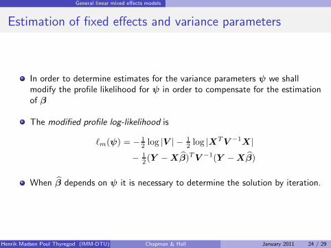
In order to determine estimates for the variance parameters ψ we shallmodify the profile likelihood for ψ in order to compensate for the estimationof β

The modified profile log-likelihood is

ℓm(ψ) = − 1

2log |V | − 1

2log |XTV −1X|

− 1

2(Y −Xβ)TV −1(Y −Xβ)

When β depends on ψ it is necessary to determine the solution by iteration.




The modification to the profile likelihood equals the so-called residualmaximum likelihood (REML)-method using the marginal distribution of the

residual (y −Xβψ).

In REML the problem of biased variance components is solved by setting thefixed effects estimates equal to the WLS solution above in the likelihoodfunction and then maximising it to find the variance component terms only.

The reasoning is that the fixed effects cannot contribute with information onrandom effects leading to a justification of not estimating these parametersin the same likelihood.

The method is also termed restricted maximum likelihood method becausethe model may be embedded in a more general model for the groupobservation vector Yi where the random effects model restricts thecorrelation coefficient in the general model.




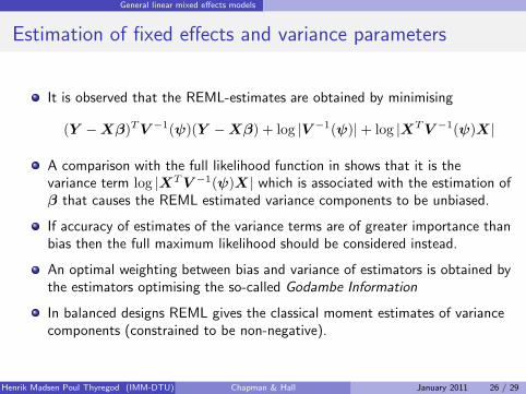
It is observed that the REML-estimates are obtained by minimising

(Y −Xβ)TV −1(ψ)(Y −Xβ) + log |V −1(ψ)|+ log |XTV −1(ψ)X|

A comparison with the full likelihood function in shows that it is thevariance term log |XTV −1(ψ)X| which is associated with the estimation ofβ that causes the REML estimated variance components to be unbiased.

If accuracy of estimates of the variance terms are of greater importance thanbias then the full maximum likelihood should be considered instead.

An optimal weighting between bias and variance of estimators is obtained bythe estimators optimising the so-called Godambe Information

In balanced designs REML gives the classical moment estimates of variancecomponents (constrained to be non-negative).



Estimation of random effects

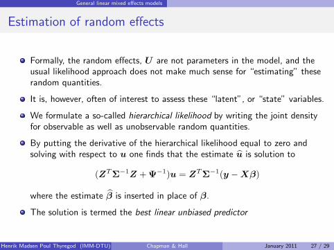
Formally, the random effects, U are not parameters in the model, and theusual likelihood approach does not make much sense for “estimating” theserandom quantities.

It is, however, often of interest to assess these “latent”, or “state” variables.

We formulate a so-called hierarchical likelihood by writing the joint densityfor observable as well as unobservable random quantities.

By putting the derivative of the hierarchical likelihood equal to zero andsolving with respect to u one finds that the estimate u is solution to

(ZTΣ−1Z +Ψ−1)u = ZTΣ−1(y −Xβ)

where the estimate β is inserted in place of β.

The solution is termed the best linear unbiased predictor



Simultaneous estimation of β and u

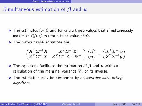
The estimates for β and for u are those values that simultaneouslymaximize ℓ(β,ψ,u) for a fixed value of ψ.

The mixed model equations are

(XT

Σ−1X XT

Σ−1Z

ZTΣ

−1X ZTΣ

−1Z +Ψ−1

)(β

u

)=

(XT

Σ−1y

ZTΣ

−1y

)

The equations facilitate the estimation of β and u withoutcalculation of the marginal variance V , or its inverse.

The estimation may be performed by an iterative back-fittingalgorithm.



Interpretation as empirical Bayes estimate

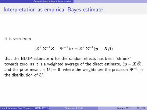
It is seen from

(ZTΣ

−1Z +Ψ−1)u = ZT

Σ−1(y −Xβ)

that the BLUP-estimate u for the random effects has been “shrunk”towards zero, as it is a weighted average of the direct estimate, (y −Xβ),and the prior mean, E[U ] = 0, where the weights are the precision Ψ

−1 inthe distribution of U .


Introduction to General and Generalized Linear …hmad/GLM/slides/lect10.pdfIntroduction to General...

Documents

Transcript of Introduction to General and Generalized Linear …hmad/GLM/slides/lect10.pdfIntroduction to General...