Introduction to G-RSM (Spectral method for dummies)

Masao Kanamitsu

Scripps Institution of Oceanography

University of California, San Diego

All the materials are available from http://g-rsm.wikispaces.com/Short+Courses

How to digitize a field

Values on grid points □ Geographical location is given□Discrete representation

Easy to understand.No computation necessary.Computer display utilize this method.

Will be referred to as physical space==========================

Notation in this presentation:Physical space in RED

Trivial 1-D example

Physical space:f(x) is expressed by 7 numbers

(-2.0, -1.33, -0.67, 0., +0.67, +1.33, +2.0)

Any other method to digitize fields?

f(x)=ax+ba=0.67b=0.

f(x) is expressed by 2 numbers (0.67, 0.)

Note Continuous representation

==========================Notation in this presentation:

Functional space in BLUE

Can we do similar procedure for more general field distributions?

Fourier Series•Combination (or summation) of sine and cosine waves with different wave length.

Born March 21, 1768Auxerre, Yonne, France

Died May 16, 1830 (aged 62)Paris, France

Nationality French Field Mathematician, physicist, and historianInstitutions École Normale

École PolytechniquePolytechniqueAcademic advisor  Joseph Lagrange

Joseph Fourier

Fourier’s discovery

He claims that any function of a variable, whether continuous or discontinuous, can be expanded in a series of sines of multiples of the variable.

Though this result is not correct, Fourier's observation that some discontinuous functions are the sum of infinite series was a breakthrough. The question of determining when a function is the sum of its Fourier series has been fundamental for centuries. Joseph Louis Lagrange had given particular cases of this (false) theorem, and had implied that the method was general, but he had not pursued the subject. Johann Dirichlet was the first to give a satisfactory demonstration of it with some restrictive conditions. A more subtle, but equally fundamental, contribution is the concept of dimensional homogeneity in equations; i.e. an equation can only be formally correct if the dimensions match on either side of the equality.

Any distribution can be expressed (approximately) by the Fourier Series

Fits better with more wave components

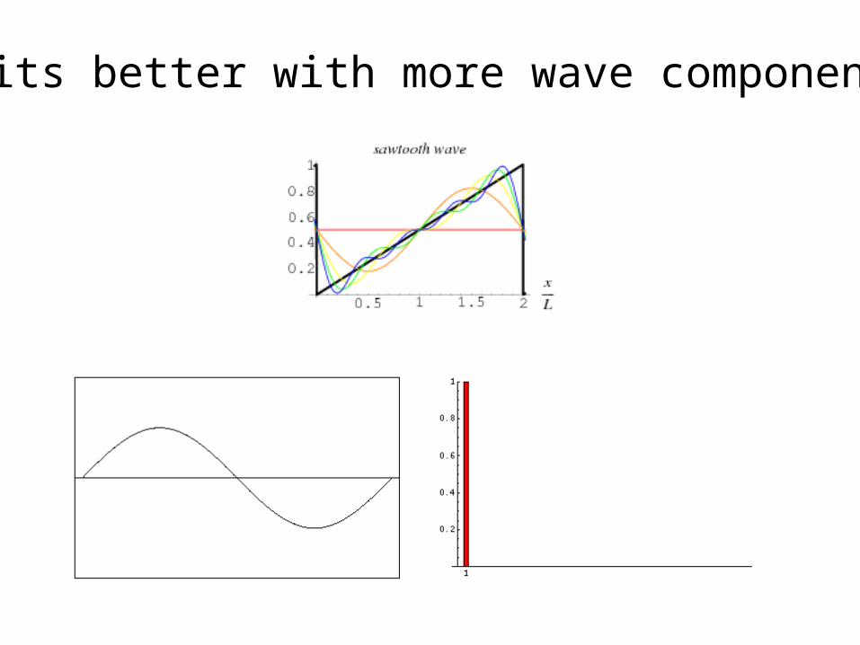
Fits better with more wave components

More general example

Physical space:f(x) is expressed by 7 numbers

(2.0, 0.0, -2.0, -0.5, 0.5, 0.0, 2.0)

Wave space:

If we use the following series of functions:

f0(x)=constantf1(x)=sin(2B/L•x), f2(x)=cos(2B/L•x),f3(x)=sin(2B/L•2x), f4(x)=cos(2B/L•2x),f5(x)=sin(2B/L•3x), f5(x)=cos(2Bx/L•3x)

then,

f(x) = 0.000 -0.772• f1(x)+1.083 • f2(x)+0.722 • f3(x)+ 0.750 • f4(x)+ 0.000 • f5(x) +0.167 • f6(x)

Now, f(x) is expressed by 7 different numbers!!

(0.000, -0.772, 1.083, 0.722, 0.750, 0.00, 0.167)

Wave space

Values of coefficients of a series of functions

Will be referred to as wave space

No geographical locationKnown set of mathematical functionsContinuous representationSpace derivatives can be computed analytically.

Not possible to visualize

grid point space

Values on grid points.

Will be referred to as grid point spaceGeographical location specifiedPhysical values themselvesDiscrete representationSpace derivatives computation requires finite difference approximation.

Easy to visualize

Derivatives Continuous vs. discrete representation

• (F/ x)x=60=(F80-F40)/(80-40)

– Can be defined only at the grid point

• (F/ x)x=60= -0.772*2/L*cos(2/Lx)- 1.083* 2/L*sin(2/Lx)+……..

Can be defined everywhere (continuous)

How to select “(series of) functions”

• Requirements:– Satisfy boundary condition– Orthogonal– Solution of a linearized forecast equation

• Examples:– 1-D periodic ==> Sinusoidal (Fourier)

– 2-D periodic over plane ==> Double Fourier

– 2-D wall (zero) ==> Sine only series

– 2-D symmetric ==> Cosine only series

– 2-D on sphere ==> Associated Legendre polynomial

Fourier Transform

Transformation between physical and wave space

1-D example:

where,

λ=2π/L

f a a m b mm

m

m

m

( ) cos sin

0

1 1

Conversion from wave space to physical space

cos sinm i m e im

f F m e im

m

( ) ( )

F mb

iam m( )

2 2

Complex notation is more convenient :

f(λ) is physical spaceF(m) is wave space

where

then

Conversion from physical space to wave space

F m f e dim( ) ( ) 1

20

2

Note that F(m) is not a function of space (λ)

f(λ) is physical spaceF(m) is wave space

Orthogonality condition

12

1

00

2

e e d for m n

for m n

im in

Horizontal derivatives

fimF m e

m

im( )( )

imF mf

e dim( )( ) 1

20

2

Physical space:

Wave space:

Note on ‘scale’

Wavenumber “m” relates to scale (spectral)

small “m” ==> large scale

large “m” ==> small scale

Think as “number of troughs and ridges around the latitude circle”

Skip spectral representation on sphere.

Please refer to the

http://g-rsm.wikispaces.com/Short+Courses

page

Spectral method and Grid-point method

A method to numerically solve linear and nonlinear (partial) differential equations.

We may have:

Spectral quasi-geostrophic model

Spectral non-hydrostatic model

Also used in pure physics and other applications

Spectral forecast equation

• Grid-point method => predict values on grids

• Spectral method => predict coefficients

Spectral Forecast Equation1-D linear equation example

),(),( tu

ct

tu

Spectral Forecast Equation1-D linear equation example

Grid-point method

2211

11 ti

ti

ti

ti uu

ct

uu

Spectral Forecast Equation1-D linear equation example

Spectral Method

12

0

2

( ) e dim

Apply the following operator to both sides of the equation

like the following:

which leads to:

deu

cdet

u imim

2

0

2

0

Spectral Forecast Equation1-D linear equation example

Spectral Method

)()(

mimcUt

mU

or, using finite differencing in time,

)(2

)()( 11

mimcUt

mUmU ttt

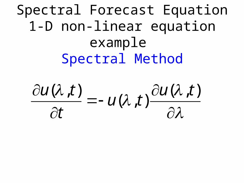
Spectral Forecast Equation1-D non-linear equation example

Spectral Method

),(

),(),( tu

tut

tu

Spectral Forecast Equation1-D non-linear equation example

Grid-point method

2211

11 ti

tit

i

ti

ti uu

ut

uu

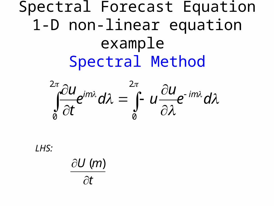
Spectral Forecast Equation1-D non-linear equation example

Spectral Method

deu

udet

u imim

2

0

2

0

LHS:

t

mU

)(

RHS:

k

im

k

ik

im

kmUkikU

deekikUu

deu

u

)()(

)(2

1

2

1

2

0

2

0

Spectral Forecast Equation1-D non-linear equation example

Spectral Method

k

kmUkikUt

mU)()(

)(

Note that his equation shows nonlinear interaction between the waves.For example, U(3) is generated by U(1) and U(2) {m=3,k=1}(or many other combinations of m and k)

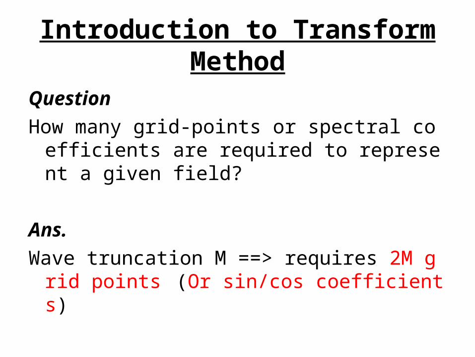
Introduction to Transform Method

Question

How many grid-points or spectral coefficients are required to represent a given field?

Ans.

Wave truncation M ==> requires 2M grid points(Or sin/cos coefficients)

QuestionHow many grid points are required to obtain ‘mathematically correct’

nonlinear term ?

Qualitative ans.Representation of u requires 2M grid pointsRepresentation of requires 2M grid pointstherefore, requires 4M grid points.

However, we have a selection rule, which states that only special combination of u and creates waves within the truncation limit, i.

e., U(k) and U(m-k). This requirement reduces the number of combinations by M-1,

x

u

x

uu

x

u

x

uuthus requires 3M+1 grid points.

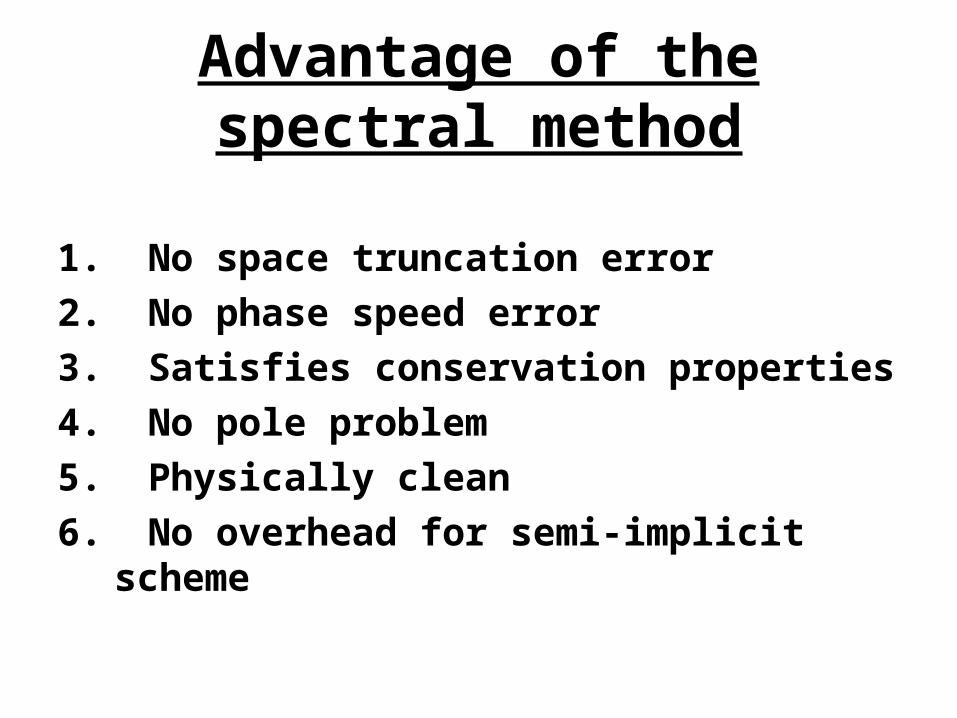
Advantage of the spectral method

1. No space truncation error

2. No phase speed error

3. Satisfies conservation properties

4. No pole problem

5. Physically clean

6. No overhead for semi-implicit scheme

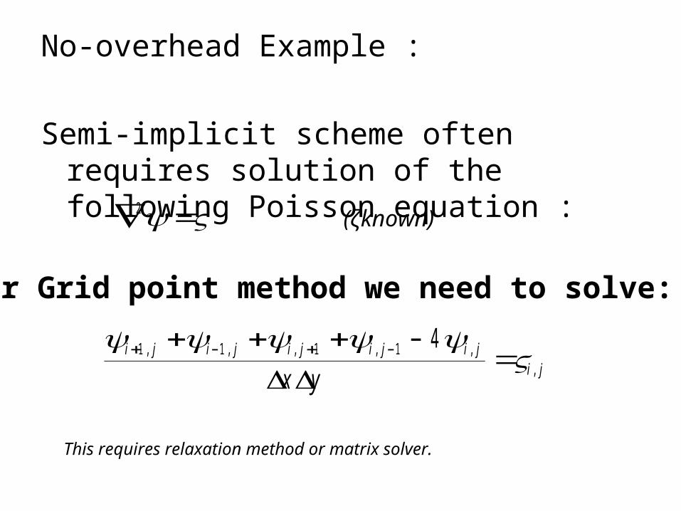
No-overhead Example :

Semi-implicit scheme often requires solution of the following Poisson equation :

2

For Grid point method we need to solve:

i j i j i j i j i j

i jx y

1 1 1 1 4, , , , ,,

(ζknown)

This requires relaxation method or matrix solver.

For Spectral method we need to solve:

n na n

mnm( )1

2 (ζknown)

Disadvantages of the spectral method

1. Restricted by boundary condition.

2. Difficulties in handling discontinuity and

positive definite quantities

==>Gibbs phenomena

3. For very high resolution (>T1000), efficiency may become a problem.

The Regional Spectral Model

Juang, H.-M. and M. Kanamitsu, 1994: The NMC nested regional spectral model.

Mon. Wea. Rev., 122, 3-26.

RSM Basics (1)

• The most serious question is “HOW TO DEAL WITH LATERAL BOUNDARY CONDITION?”– Assume cyclic .... Hilam– Assume zero .... Tatsumi– (Non-zero boundary condition also causes serio

us difficulties when semi-implicit scheme is used.)

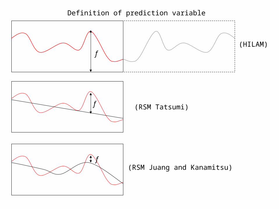
(HILAM)

(RSM Tatsumi)

(RSM Juang and Kanamitsu)

Definition of prediction variable

f

f

f

RSM Basics (2)

Introduction of the Perturbation

1. Satisfy zero lateral boundary condition2. Better boundary condition for semi-implicit

scheme3. Diffusion can be applied to perturbation only

(does not change large scale).4. Lateral boundary relaxation cleaner.5. Maintain large scale forecast produced by the

global model

RSM Basics (3)

Definition of perturbation

At=Ar+Ag

At: Full field (to be predicted)

Ar: Perturbation (rsm variable, to be predicted)

Ag: Global model field (known at all times)

RSM Basics (4)

Writing equation for Ar is not easy, particularly for nonlinear terms and very nonlinear physical processes.

y

AAvv

x

AAuu

t

A

t

A grgr

grgr

gr)(

)()(

)(

RSM Basics (5)Different approach:

t

At

Compute using At=Ar+Ag, then use

t

A

t

A

t

A gtr

t

At

is computed in a similar manner as regular model.

t

Ag

is known

Step by step computational procedure (1)

1. Run global model. Get global spherical coefficient Ag(n,m) at all times.

2. Get grid point analysis over regional domain At(x,y).

3. Get grid point values of global model.Ag(n,m) ==> Spher. trans. ==> Ag(x,y)

4. Compute grid point perturbation Ar(x,y) =At(x,y) - Ag (x,y)

• Get Fourier coefficient of perturbation.Ar(x,y) ==>Fourier trans. ==> Ar(k,l)

(Now Ar(k,l) satisfies zero b.c.)[Steps 1-5 are preparation at the initial time]

Step by step computational procedure (2)

6. Get grid point value of perturbation and its derivatives.

Ar(k,l) ==>Fourier trans. ==> Ar(x,y)

Ar(k,l) ==>Fourier trans.==>

Ar(k,l) ==>Fourier trans.==>

7. Get grid point value of global field and its derivatives.

Ag(m,n) ==>Spherical tans.==> Ag(x,y)

Ag(m,n) ==>Spectral trans.==>

Ag(m,n) ==>Spectral trans.==>

y

yxAr

),(

x

yxAr

),(

x

yxAg

),(

y

yxAg

),(

Step by step computational procedure (3)

8. Get grid point total field and derivativesAt (x,y)= Ag(x,y) + Ar(x,y)

x

yxA

x

yxA

x

yxA rgt

),(),(),(

y

yxA

y

yxA

y

yxA rgt

),(),(),(

9. Now possible to compute full model tendencies in grid point space

y

AAvv

x

AAuu

t

A grgr

grgr

t)(

)()(

)(

(This is non-zero at the boundary)

Step by step computational procedure (4)

10. Get perturbation tendency

t

A

t

A

t

A gtr

(Note that

t

Ag

is known)

11. Get Fourier coefficient of perturbation tendency

t

lkA

t

A rr

),( (This satisfies boundary condition)

Step by step computational procedure (5)

12. Advance in time

tt

lkAlkAlkA r

ttrttr

2

),(),(),(

13. Go back to step 6

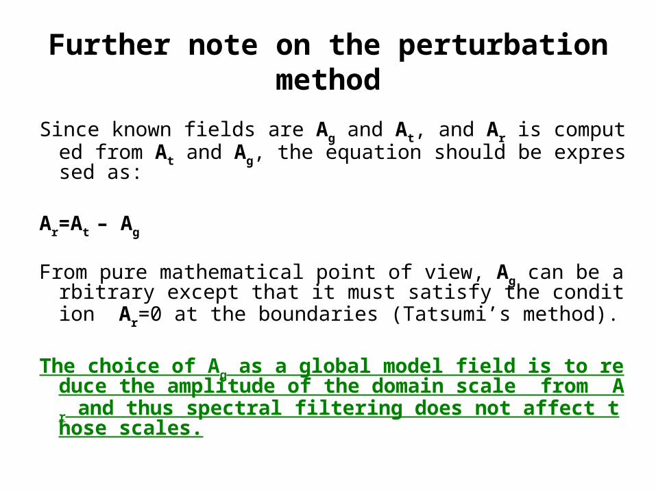
Further note on the perturbation method

Since known fields are Ag and At, and Ar is computed from At and Ag, the equation should be expressed as:

Ar=At – Ag

From pure mathematical point of view, Ag can be arbitrary except that it must satisfy the condition Ar=0 at the boundaries (Tatsumi’s method).

The choice of Ag as a global model field is to reduce the amplitude of the domain scale from Ar and thus spectral filtering does not affect those scales.

Further note on the perturbation method

Since RSM does not directly predict Ar, it may not be appropriate to call it as a perturbation model.

More appropriately, it should be called a perturbation filter model.

Although the global model field is used in the entire domain, it is only applied to reduce the error due to the Fourier transform of the domain scale field. There is no explicit forcing towards global model field in the interior of the regional domain.

The explicit forcing towards the global model fields is achieved by the lateral boundary blending and/or nudging. It is important to note that these lateral boundary treatment is still an essential part of the RSM, as in the grid-point regional model.

The use of Scale Selective Bias Correction Method developed recently by Kanamaru and Kanamitsu considers nudging inside the domain to reduce large systematic error. (To be discussed in other talks)

Little history

1970-‘85: Global spectral modelBourke(1974), Hoskins & Simmons (1975)ECMWF, NMC, JMA

1980's: Regional spectral modelTatsumi(1986)Hoyer (and Simmons) (1987)Juang and Kanamitsu (1994)

Spherical transform

)( mn

immn PeY

mnP

Y nm Spherical harmonic function

m: zonal wavenumbern: total wavenumbern-m: number of zero crossings

is Associated Legendre Polynomial

(Φ is latitude) 2

First few examples of mnP

P

P

P

P

P

P

P

0

0

1

0

1

1

2

0 2

2

1

2

1 2

3

0 3

1

12

3 1

3

3

12

5 3

cos

sin

( cos )

sin cos

sin

( cos cos )

Properties of the

1) Defined as a solution of on sphere.

2) Function of sin2 and cos2.

3) Largest order is ‘n’.

4) for m>n

5) Has n-m zero crossing between the poles.

6) Symmetric w.r.t. equator for even n-m.

7) Antisymmetric w.r.t. equator for odd n-m.

8) Orthogonal function.

mnP

02 f

0mnP

Legendre (or spherical) Transform formula

f F n m P enm

nm

im( , ) ( , ) ( )

0

F n m f e Pimn

m( , ) ( , ) (cos )

14

1

1

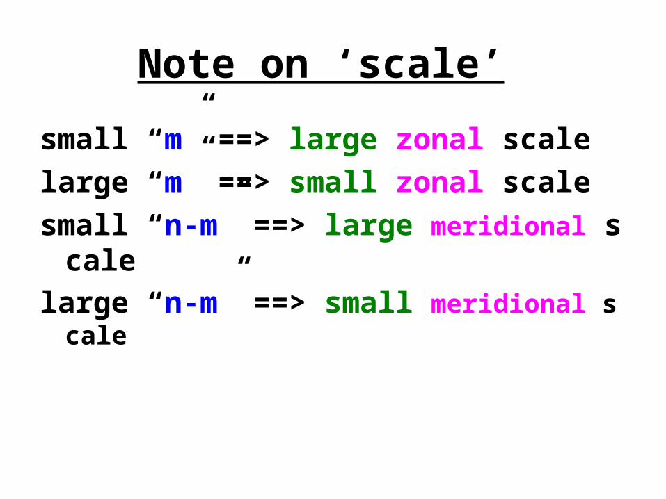
Note on ‘scale’

small “m” ==> large zonal scale

large “m” ==> small zonal scale

small “n-m” ==> large meridional scale

large “n-m” ==> small meridional scale

Truncation (model resolution)

• 1-D example:• ‘Maximum m’ or ‘M’ determines the

smallest scale possible.• 2-D spherical example

n

m

N

M

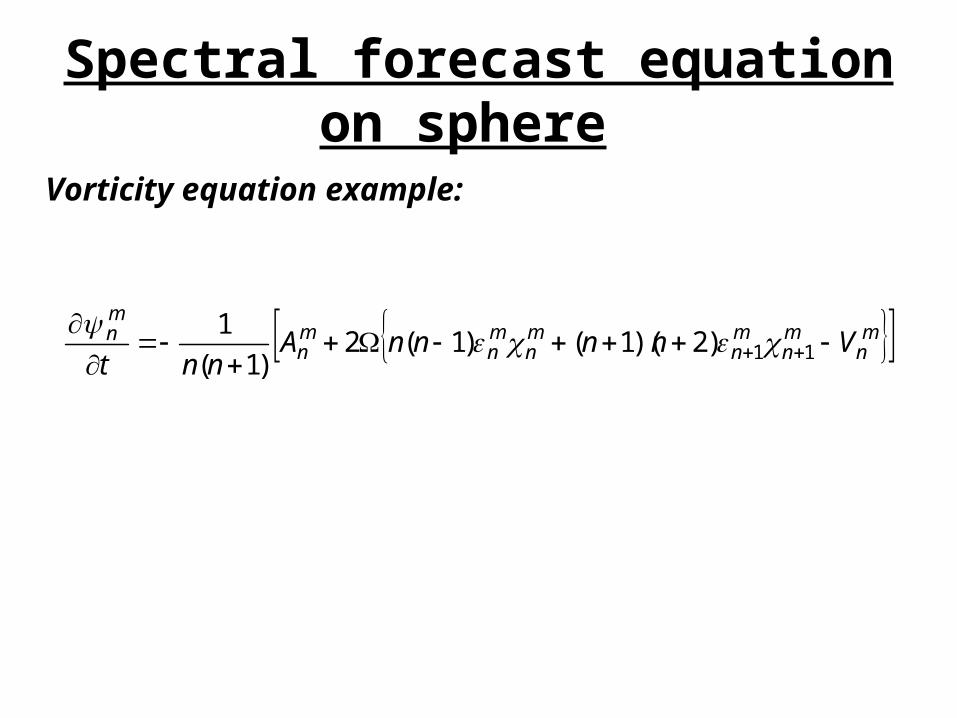
Spectral forecast equation on sphere

Vorticity equation example:

mn

mn

mn

mn

mn

mn

mn VnnnnA

nnt

11)2)(1()1(2)1(

1

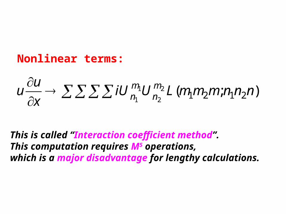
Nonlinear terms:

);( 21212

2

1

1nnnmmmLUiU

x

uu m

nmn

This is called “Interaction coefficient method”.This computation requires M5 operations,which is a major disadvantage for lengthy calculations.

“How many grid points are required to obtain ‘mathematically accurate’ nonlinear term?”

- another derivation -

Problem is that sampling interval misinterprets correct wavelength.

Sampled here

f x F S R eS R j

i S RS

j

( )

( )2

21

If we have 2*S gridpoints. We can represent S waves. Suppose, we have a wave with a wavenumber S+R, then the grid point values of this wave on 2*S grid points are expressed as:

The Fourier transform of this grid point value to wavenumber will be preformed as:

F mS

f x ejj

S imS

j( ) ( )

( )

12 1

2 2

21

F mS

F S R ei j

S R m

S

j

S

( ) ( )( ) ( )

1

2

1 22

1

2

This summation is non-zero if:

S+R-m is an integer multiple of 2S or m=-{(2N-1)S-R} where N=1,2,3,4...

When N=1, |m|=S-RN=2, |m|=3S-R (greater than S for R<S thus no need

to consider for N>1)

This indicates that the wave S+R is aliased to S-R. In other word, aliasing occurs as if the wave is folded to a smaller wavenumber at S.

aliasing of S+R to S-R:

SS-R S+R

The quadratic term generates 2M wave. If we place a condition to the number of grid points (2S) such that the waves between M+1 and 2M do not aliased into waves less than or equal to M, then we have a condition, S+R=2M and S-R=M, i.e.,

132 MS (+1 to avoid aliasing to M)

thus requires 3M+1 grid points.

For spherical coefficients, number of required E-W grid points are:

(3M+1)

and N-S grid points are:

(3M+1)/2

for triangular truncation.

Note:We choose number of grid points in E-W so that the Fast Fourier Transform

works the best. It requires that the number of points is a multiple of 2, 3, 5. Combination of this restriction and the condition above determines the most efficient model truncation (T21, T42, T63 ...). Note that NCEP model has additional restriction that the wavenumber must be even).Example: Number of grid point = 128 = 2**7

3M+1=128 ==> M=42

There is additional requirement for the non-linear term calculations on sphere!!

N-S grid point placement must satisfy the following equation which makes the numerical error of the integration zero.

f x dx W f xk kk

J

( ) ( )

11

1

ε=0 leads to:

P for triang truncationM( ) ( ) . .3 1

2

0 0

These special latitudes are called Gaussian latitudes

Example for M=5

P x x x

x

80 8 6 4

2

1128

6435 12012 6930

1260 35 0

(

) .