Introduction to Design Optimization

James T. Allison

University of Michigan, Optimal Design LaboratoryJune 23, 2005

1 Introduction

Technology classes generally do a good job of helping students learn analysistechniques, i.e. methods for predicting the behavior of some artifact. Infact, sophisticated tools such as finite element analysis have been introducedin technology classes. Certainly predictive capabilities are valuable, but forwhat exactly? Predictive tools allow us to model in the virtual world thingsthat exist in the physical world. Without modeling, we would be forced torely on full-scale prototypes, which may:

• be to expensive to build more than one

• require substantial time for each realization

• risk human safety during testing

Suppose you are an engineer working for a company that produces somewidget, and you modeled this widget and predicted its performance. Maybeit is expected to be safe, or perhaps it is predicted to fail. In either case,what do you do next? What questions should you ask?

Safe prediction: Can we improve performance or reduce cost without risk-ing failure?

Failure prediction: How can we change the widget in order to preventfailure?

1

What common thing does each question seek? In either case, a change inthe characteristics, or design, of the product is sought. A new design needsto be proposed that we hope performs better than the last design. What aresome ways to generate new and improved designs? The first two suggestionsemploy a trial-and-error approach:

• Use intuition or experience-based knowledge to propose a new design

• Change one aspect of the product at a time and see what happens

Each approach will require iteration, and even if this iteration is per-formed in the less expensive and more safe virtual world, we may not arriveat the results we want as quickly as we would like. We may end up testinga large portion of the set of possible designs, and at the end still not know ifthere exists some other design that might still be better. In addition, manymodern products, such as computers or automobiles, are so complex that nosingle person is capable of possessing the intuition required to progress to-ward more ideal designs. A more scientific approach is needed. Optimization,a branch of mathematics, provides the necessary tools to move efficiently to-ward a design that is superior to all other alternatives. This course providesan introductory overview of design optimization, and motivates its use insecondary education curricula.

2 Example 1: Optimal Design of a Trebuchet

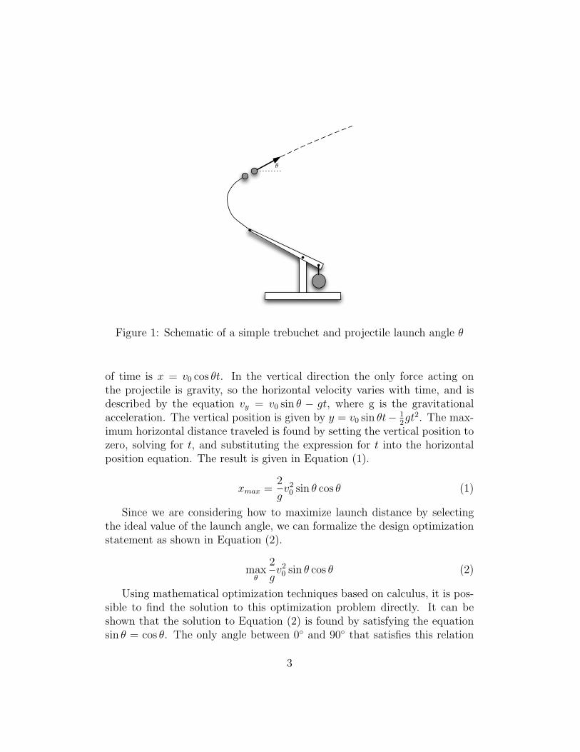
We begin with the first of two computational examples, the design of a tre-buchet, in order to introduce some basic concepts and to further motivatethe study of design optimization. A trebuchet, which launches a projectileusing only force from a weight, is frequently the object of student designprojects. A design objective might be to maximize the distance a projectileis launched, subject to some kind of limitations on the design such as size,weight, or building materials. An important aspect of trebuchet design isthe launch angle θ of the projectile (Figure 1). Projectile motion is a clas-sical topic usually studied in high-school physics, and we can use the basicequations of projectile motion to predict how far an object will be launchedfor a given launch angle and launch speed.

Neglecting air resistance, the horizontal component of the projectile ve-locity is constant, so vx = v0 cos θ, and the horizontal position as a function

2

θ

Figure 1: Schematic of a simple trebuchet and projectile launch angle θ

of time is x = v0 cos θt. In the vertical direction the only force acting onthe projectile is gravity, so the horizontal velocity varies with time, and isdescribed by the equation vy = v0 sin θ − gt, where g is the gravitationalacceleration. The vertical position is given by y = v0 sin θt− 1

2gt2. The max-

imum horizontal distance traveled is found by setting the vertical position tozero, solving for t, and substituting the expression for t into the horizontalposition equation. The result is given in Equation (1).

xmax =2

gv2

0 sin θ cos θ (1)

Since we are considering how to maximize launch distance by selectingthe ideal value of the launch angle, we can formalize the design optimizationstatement as shown in Equation (2).

maxθ

2

gv2

0 sin θ cos θ (2)

Using mathematical optimization techniques based on calculus, it is pos-sible to find the solution to this optimization problem directly. It can beshown that the solution to Equation (2) is found by satisfying the equationsin θ = cos θ. The only angle between 0◦ and 90◦ that satisfies this relation

3

is 45◦. Without knowledge of the optimization techniques that led to thisanswer, how might a designer approach this problem? One might use somesoftware like MS ExcelTMto rapidly calculate the launch distance for a givenangle, or even to graph the relationship between θ and xmax and visuallyfind the optimum. Figure 2 illustrates how MS ExcelTMcan be used for theseinvestigations. This works fine for such a simple example, but what happensif each function evaluation requires minutes, hours, or even days (as may bethe case with finite element analysis or computational fluid dynamics)? Or,what if more than two items are being varied at a time in the design and it isimpossible to visualize where the optimum is? A more intelligent approachis required in these cases.

An expansive array of optimization algorithms have been developed tosolve equations such as the one shown in Equation 2. MS ExcelTMhas anadd-in package called Solver that employs some of these algorithms to solvesuch problems. By defining the which values are to varied, what should beoptimized, and what constraints might exist, these algorithms can automat-ically find the best design, even if the number of design variables is large.

This course will explore in a little more depth what design optimizationis, how to formulate optimization problems, and some additional extensionsfor optimization. Figure 3 provides a definition and framework for the restof the course.

4

Example 1: Trebuchet Launch Angle Optimization

g 9.81

! 45

v0 15

xmax 22.9357798

Trajectory Visualization

x y

0 0

1 0.9564

2 1.8256

3 2.6076

4 3.3024

5 3.91

6 4.4304

7 4.8636

8 5.2096

9 5.4684

10 5.64

11 5.7244

12 5.7216

13 5.6316

14 5.4544

15 5.19

16 4.8384

17 4.3996

18 3.8736

19 3.2604

20 2.56

21 1.7724

22 0.8976

23 -0.0644

Launch Angle-Launch Distance Relationship

! xmax

0 0

5 3.98275637

10 7.8444987

15 11.4678899

20 14.7428351

25 17.5698267

30 19.862968

35 21.552583

40 22.5873338

45 22.9357798

60 19.862968

70 14.7428351

80 7.8444987

90 2.8088E-15

Projectile Trajectory

0

1

2

3

4

5

6

7

0 5 10 15 20 25

Horizontal Position (m)

Verti

cal

Po

sit

ion

(m

)

xmax

0

5

10

15

20

25

-10 10 30 50 70 90

Figure 2: Using MS ExcelTMto determine the optimal launch angle.

5

Effective and efficient decision making based on quantitative metrics

'Making the right decision'

'Making decisions quickly'

'What decisions should be made'

Algorithms and

Convergence

Problem Formulation

Optimality Conditions

'Quantifiably predict the outcome of a

decision'

Governing Equations

Numerical Approximations

Empirical Models

Design variables vs. parameters

Finding the best design without testing them all

Optimization:

Figure 3: Definition of optimization

6

3 Making Effective Design Decisions

In design optimization we seek the design that is superior to all others. Theway we judge this superiority depends on how the problem is formulatedand how the quantitative metrics for comparison are obtained. This sectiondiscussed the first item, while the latter pertains to modeling, and is discussednext. Optimization problems may be described in a standard form called thenegative null form:

minx

f(x) (3)

subject to g(x) ≤ 0

h(x) = 0

The objective is always posed as a minimization problem (a maximizationproblem can be transformed to minimization by negating the objective func-tion), and constraints are grouped into inequality and equality constraints.The vector x is comprised of all design variables, i.e., values that are to bechanged during the optimization process. Any input values that are heldfixed during the optimization process are called design parameters. The ob-jective and constraint functions are all dependent on x. The way we chooseto formulate the problem will affect the resulting solution. For example, ifwe are designing a car, we might want to minimize both 0 − 60 time andfuel consumption. We could use fuel economy as the objective and minimumacceleration as a constraint, or acceleration as the objective and minimumfuel economy as a constraint. The mathematical techniques will help us findthe answer, but we are the ones that define the problem. The answer to thedesign optimization problem is only as good as the problem definition andthe models used in the solution.

Now that we know formally what the problem is, how do we define whensomething is optimal? Refer back to the θ vs. xmax plot in Figure 2. What doyou observe about the optimal point? The slope of the function at that pointis zero, or in other words a line tangent to the curve at the optimal pointis horizontal. This is a necessary condition for optimality. This idea can beextended to higher dimensions using calculus, and these optimality conditionsare the basis for many optimization algorithms. Other more complicatedconditions can be investigated to determine whether or not we can guaranteethat a design is optimal.

7

Many examples exist in nature of making ideal or optimal ‘design’ de-cisions. A general principle of natural systems is to seek the lowest energystate. Chemical reactions proceed only if they are energetically favorable.Soap bubbles are round because of the energy associated with surface area,and a spherical bubble has the smallest surface area for a given volume ofcontained air. In addition, a single large bubble has less surface area thanmany smaller bubbles with the same collective volume, explaining why soapbubbles in you sink tend to coalesce. Crystals form based on similar prin-ciples. If minerals or metals are allowed to cool slowly, the crystals tend tobe larger and the total interfacial area between crystals will be smaller. Sur-vival of the fittest phenomena in nature in effect optimizes organisms or entireecosystems, and in fact a class of algorithms is based on these evolutionaryprocesses.

4 Making Design Decisions Quickly

Now that we have defined more carefully what an optimal design is, we candiscuss how to find this design more quickly. Earlier we described how theset of possible designs can be described as a curved function (Figure 2). Thisidea extends to higher dimensions. If we have two design variables instead ofjust one, the objective function will be a surface. Suppose we are in a fishingboat on a pond and we want to find the lowest point of the pond. We cannotsee the bottom, so the only information we have is the depth at individuallocations. We could use trial and error, but that could take a very long time.Another approach would be to create a grid and measure each point on thegrid, but then we will never be sure if another point exists that might belower. What is a better approach to finding the lowest point? We ideal wantto find the lowest point, without having to test all points. Suppose at eachpoint we take a few measurements nearby the original measurement point.This will give us some idea of the slope of the bottom surface of the pond,and what is the downhill, or steepest descent, direction. We then head thatdirection, taking measurements along the way, until we find the lowest pointin that direction. Then we take some extra measurements there to determinethe downhill direction, and repeat the process until we discover there is nomore downhill direction. At that point we have met the necessary conditionsfor optimality, and stop the process.

This steepest descent method works well for many optimization prob-

8

lems. It converges quickly in many cases, and is simple to implement. Othermore sophisticated algorithms that can converge even more quickly exist thatare still based on information about slope and downhill direction. The ex-istence and rate of convergence are important properties of an optimizationalgorithm. Existence of convergence means that the algorithm will termi-nate (ideally at the optimal point), and rate refers to how many functionevaluations, or measurements, must be made before convergence occurs.

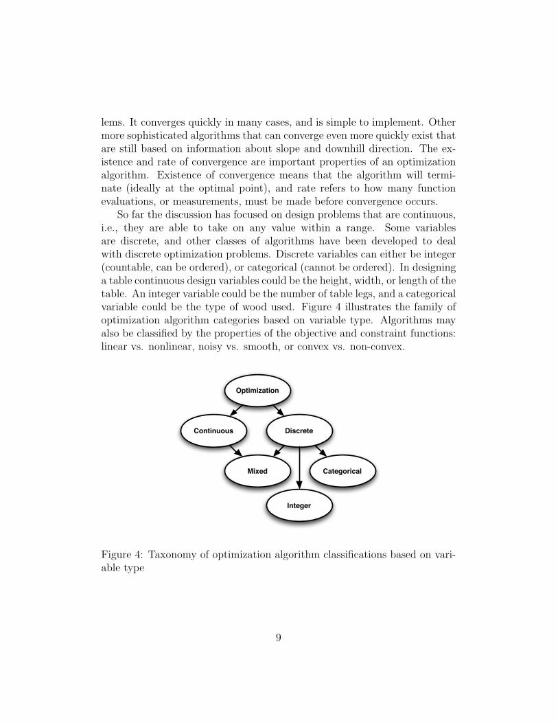
So far the discussion has focused on design problems that are continuous,i.e., they are able to take on any value within a range. Some variablesare discrete, and other classes of algorithms have been developed to dealwith discrete optimization problems. Discrete variables can either be integer(countable, can be ordered), or categorical (cannot be ordered). In designinga table continuous design variables could be the height, width, or length of thetable. An integer variable could be the number of table legs, and a categoricalvariable could be the type of wood used. Figure 4 illustrates the family ofoptimization algorithm categories based on variable type. Algorithms mayalso be classified by the properties of the objective and constraint functions:linear vs. nonlinear, noisy vs. smooth, or convex vs. non-convex.

Optimization

Continuous Discrete

Integer

Mixed Categorical

Figure 4: Taxonomy of optimization algorithm classifications based on vari-able type

9

5 What Decisions are to be Made?

We previously introduced the design vector x, which is a set of numbers rep-resents a design. Describing a design completely by a set of numbers maybe a new idea for some individuals. Initial design stages where the basicconfiguration of a design is generated is sometimes called conceptual design.Once this conceptual design is determined, it can be described completely bya set of numeric parameters and relations between these parameters. Thisis sometimes referred to as parametric design. An example of parametricdesign is a CAD drawing that has been created using relations between im-portant dimensions such that if a change is made to any of these dimensions(or parameters), the rest of the design is automatically updated. It is desir-able to minimize the number of parameters used to describe a design. Whenwe consider how to formulate the design optimization problem, an impor-tant decision is what parameters to select as design variables (values thatare changed in the optimization process), and what parameters should beleft fixed as design parameters. It is easier to solve a problem with fewerdesign variables, but limiting the number of design variables may cause usto overlook certain designs that may be more desirable.

6 Modeling: Quantification of Designs

A critical link exists between the success of a design optimization endeavorand the models (or analysis) used in solving the optimization problem. Theaccuracy of design optimization solution is only as accurate as the mod-els used to represent the artifact. This motivates the usage of high-fidelitymodels. However, these models are computationally expensive. A designermay not have enough time to wait for such an optimization to finish. Thistradeoff is difficult to make. One approach is to perform preliminary opti-mization studies using simple models in order to narrow down the number ofdesign configurations and design variables, and then move on to high-fidelitymodeling for final optimization.

7 Example 2: Air Flow Sensor Design

The second example considers the design of an air flow sensor. A spring-loaded panel of length ` and width w deflects as air flows past it. The amount

10

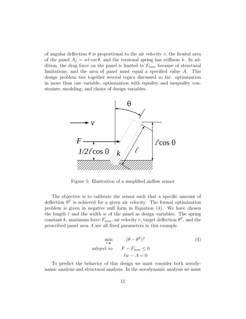
of angular deflection θ is proportional to the air velocity v, the frontal areaof the panel Af = w` cos θ, and the torsional spring has stiffness k. In ad-dition, the drag force on the panel is limited to Fmax because of structurallimitations, and the area of panel must equal a specified value A. Thisdesign problem ties together several topics discussed so far: optimizationin more than one variable, optimization with equality and inequality con-straints, modeling, and choice of design variables.

v

cos k

F1/2 cos

Figure 5: Illustration of a simplified airflow sensor

The objective is to calibrate the sensor such that a specific amount ofdeflection θT is achieved for a given air velocity. The formal optimizationproblem is given in negative null form in Equation (4). We have chosenthe length ` and the width w of the panel as design variables. The springconstant k, maximum force Fmax, air velocity v, target deflection θT , and theprescribed panel area A are all fixed parameters in this example.

min`,w

(θ − θT )2 (4)

subject to F − Fmax ≤ 0

`w − A = 0

To predict the behavior of this design we must consider both aerody-namic analysis and structural analysis. In the aerodynamic analysis we must

11

predict the drag force given the air velocity and frontal area of the panel.Using a simple analysis technique, Equation (5) provides us with the meansto quantify this relationship. C is a constant that is related to the dragcoefficient of the panel and the density of air.

F = CAfv2 = C`w cos θv2 (5)

In the structural analysis we need to determine the deflection as a functionof drag force. Assuming the spring is linear, Equation (6) approximatesthis relationship. Note that we cannot solve explicitly for θ, so a numericalmethod must be employed in the structural analysis.

kθ =1

2F` cos θ (6)

The structural and aerodynamic analyses are interdependent, i.e., theoutput of the structural analysis is the input to the aerodynamic analysis,and vice-versa. This can be overcome using a recursive solution process suchas fixed point iteration. A guess is made for the value of one of the inputs tostart the process. Let’s say we choose to guess a value for the deflection inorder to execute the aerodynamic analysis. This produces an approximationfor the drag force, which is then used as an input to the structural analysis togenerate an updated value for the deflection. This process is repeated untilthe coupling variables, θ and F , converge to stable values. Figure 6 illustratesthe information flow between the two different disciplinary analyses.

StructuralAnalysis

AerodynamicAnalysis

l

l,w

F

Figure 6: Information flow between structural and aerodynamic analyses

12

Table 1: Parameter values used for the air flow sensor problemparameter value units

θT 0.25 radiansFmax 7.0 newtons

A 0.01 metersk 0.50 newtons/radianC 1.0 kilograms/meter3

v 40 meters/second

In order to visualize the space of feasible designs and the correspondingperformance, the objective and constraint functions were computed over arange of width and length values, and plotted in Figures 7 and 8. Theparameter values used are shown in Table 1.

Figure 7 allows us to visualize the nature of the objective function. Ob-viously small values of ` do a good job of minimizing the objective, but weneed to be mindful of constraints. Figure 8 illustrates the constraints. Wemust stay on the solid line, which represents the equality constraint, andon the upper right side of the dashed line, which represents the inequalityconstraint. Observing the downhill directions, we see that the optimal designexists at the intersection of these two constraint lines.

The graphical approach to solving the air flow sensor problem is instruc-tive, but can be time consuming and uses up unnecessary resources. We canidentify the optimum design with far fewer analysis evaluations, and in muchless time using one of the many available software tools.

8 Summary of Basic Topics

The primary value of optimization in a product design context is that isenables us to find to best possible design in a relatively small amount of time.However, there are limitations to optimization techniques. The ‘optimaldesign’ is only optimal with respect to how the problem was formulated,to what values were chosen as design variables, and to the accuracy of themodeling used. A practitioner needs to ask the following questions:

• Does the objective function accurately reflect what is really wanted?

• Is the modeling accurate enough.

13

00.1

0.20.3

0.40.5

-0.02

0

0.02

0.04

0.06

0

0.5

1

1.5

2

2.5

l

Airflow Sensor Design Space

w

Figure 7: Three-dimensional view of the air flow sensor objective function.

0 0.05 0.1 0.15 0.2 0.25 0.3 0.35 0.4 0.45 0.5-0.02

-0.01

0

0.01

0.02

0.03

0.04

0.05

0.06

l

w

Contour Plot of Design Space

Figure 8: Contour lines of the objective function and constraints. Equalityconstraint is the solid line, and the inequality constraint is the dashed line.

14

• Are there constraints or interactions in the real physical design thatwere overlooked in the formulation of the optimization problem?

• Is there uncertainty or variation in:

– Manufacturing processes or supplies?

– Product usage?

– Environment the product exists in?

– Modeling or analysis?

9 Additional Topics

This section outlines additional topics for potential discussion, which may becovered as time permits.

1. Organizations and Economies as optimization processes

2. Complex system optimization

(a) Analytical Target Cascading: coordinating between system-leveland component-level thinking

(b) Multidisciplinary Design Optimization: integration of many dif-ferent disciplinary analysis into an overall system optimization

(c) Software for large-scale optimization: Optimus, iSIGHT

3. Additional optimization applications

(a) Fitting models to experimental results

(b) Design of experiments

(c) Operations Research: military operations planning, airport prob-lem, diet problem, project management

(d) Manufacturing: optimization of CNC tool paths, tolerance alloca-tion

4. Multi-objective optimization

5. Product family/product platform design

15

6. Local vs. global optima

7. Generalized reduced gradient method (algorithm used in MS ExcelTM)

16