
Introduction to density-functional theory · Preface This is an introductory course on density...
121
Introduction to density-functional theory Robert van Leeuwen May 21, 2014
Transcript of Introduction to density-functional theory · Preface This is an introductory course on density...

Introduction to density-functional theory
Robert van Leeuwen
May 21, 2014

2

Preface
This is an introductory course on density functional theory intended for students with a basicbackground in quantum mechanics. Density functional theory (DFT) is presently one of the mostheavily used approaches to calculate properties of many-electron systems, such as molecules andsolids. The main reason for this is that the theory allows for an exact way to map the interactingmany-body problem to an effective non-interacting one in which the effective potential dependsfunctionally on the particle density. Having an effective non-interacting system is very advanta-geous from a computational point of view. Furthermore it is, from a conceptual viewpoint, veryinteresting to see that there exists an exact one-particle picture of an interacting many-particlesystem. However, there is a price to be paid for these simplifications. The effective potential inthe one-particle equations depends in a complicated way on the particle density and the basictheorems of DFT do not provide insight into the ways of finding sufficiently accurate and usefulapproximations that can be used in practice. Nevertheless, it has turned out that relativelysimple approximations have already been very successful and has allowed useful predictions ofthe properties of many-electron systems, in close agreement with experimental results. However,there have also been notable failures in certain cases and therefore there is a strong need forimprovements, which is the topic of much current research. It is the goal of these lecture notesto give an overview of the basic theory, both for ground state and time-dependent systems, aswell as of the several approaches that have been used to develop approximate density functionals.The notes start with some basic concepts in quantum mechanics and then discusses many-particlesystems. Then we move towards a discussion of the physical meaning of reduced quantities suchas densities and density matrices and start with a discussion of basic underlying theorems ofDFT, notably the Hohenberg-Kohn theorem and its extensions. We then have a long discus-sion on approximate density functionals and move then to the topic of time-dependent densityfunctional theory.
i

ii PREFACE

Contents
Preface i
1 Quantum mechanics of many particles 11.1 One-particle quantum mechanics . . . . . . . . . . . . . . . . . . . . . . . . . . 1
1.1.1 Quantum states and the bra and ket vectors . . . . . . . . . . . . . . . . 11.1.2 Observables and linear operators . . . . . . . . . . . . . . . . . . . . . . 71.1.3 Quantum dynamics and the Schrödinger equation . . . . . . . . . . . . . 91.1.4 Rotations and electron spin . . . . . . . . . . . . . . . . . . . . . . . . . 14
1.2 Many-particle quantum mechanics . . . . . . . . . . . . . . . . . . . . . . . . . 231.2.1 Indistinguishable particles . . . . . . . . . . . . . . . . . . . . . . . . . . 231.2.2 Field operators . . . . . . . . . . . . . . . . . . . . . . . . . . . . . . . . 271.2.3 General basis states . . . . . . . . . . . . . . . . . . . . . . . . . . . . . 311.2.4 The many-particle Hamiltonian . . . . . . . . . . . . . . . . . . . . . . . 34
2 Density and density matrices 392.1 Correlation functions . . . . . . . . . . . . . . . . . . . . . . . . . . . . . . . . 39
2.1.1 The particle density . . . . . . . . . . . . . . . . . . . . . . . . . . . . . 392.1.2 The pair density and other correlation functions . . . . . . . . . . . . . . 42
2.2 Density matrices . . . . . . . . . . . . . . . . . . . . . . . . . . . . . . . . . . . 442.2.1 General properties . . . . . . . . . . . . . . . . . . . . . . . . . . . . . . 442.2.2 Expectation values . . . . . . . . . . . . . . . . . . . . . . . . . . . . . 47
2.3 Correlation functions revisited . . . . . . . . . . . . . . . . . . . . . . . . . . . . 472.3.1 Noninteracting states . . . . . . . . . . . . . . . . . . . . . . . . . . . . 472.3.2 A two-particle example . . . . . . . . . . . . . . . . . . . . . . . . . . . 49
3 The Hohenberg-Kohn theorem 513.1 Ground state and Rayleigh-Ritz principle . . . . . . . . . . . . . . . . . . . . . . 513.2 The Hohenberg-Kohn mappings . . . . . . . . . . . . . . . . . . . . . . . . . . . 523.3 The Hohenberg-Kohn variational principle . . . . . . . . . . . . . . . . . . . . . 533.4 Constrained search and domain questions . . . . . . . . . . . . . . . . . . . . . 54
3.4.1 v-representability . . . . . . . . . . . . . . . . . . . . . . . . . . . . . . 543.4.2 Domain extensions . . . . . . . . . . . . . . . . . . . . . . . . . . . . . 54
4 The Kohn-Sham construction 574.1 Derivation of the Kohn-Sham equations . . . . . . . . . . . . . . . . . . . . . . 57
4.1.1 The Hellman-Feynman theorem . . . . . . . . . . . . . . . . . . . . . . . 594.1.2 The coupling constant integration . . . . . . . . . . . . . . . . . . . . . 60
4.2 The local density approximation . . . . . . . . . . . . . . . . . . . . . . . . . . 624.2.1 The homogeneous electron gas . . . . . . . . . . . . . . . . . . . . . . . 624.2.2 The Kohn-System for the homogeneous electron gas . . . . . . . . . . . 62
iii

iv CONTENTS
5 Orbital functionals and response functions 675.1 Functional derivatives of orbital functionals . . . . . . . . . . . . . . . . . . . . 67
5.1.1 Example: The exchange potential . . . . . . . . . . . . . . . . . . . . . 695.2 Static response functions . . . . . . . . . . . . . . . . . . . . . . . . . . . . . . 70
5.2.1 The static exchange-correlation kernel . . . . . . . . . . . . . . . . . . . 705.2.2 The static exchange kernel . . . . . . . . . . . . . . . . . . . . . . . . . 72
6 The gradient expansion 776.1 The functional Taylor expansion of the xc-energy . . . . . . . . . . . . . . . . . 77
6.1.1 A consistency condition . . . . . . . . . . . . . . . . . . . . . . . . . . . 796.1.2 Polynomial structure of the response functions . . . . . . . . . . . . . . . 806.1.3 The gradient expansion . . . . . . . . . . . . . . . . . . . . . . . . . . . 846.1.4 Example 1: The gradient expansion for the kinetic energy . . . . . . . . . 886.1.5 Example 2: The gradient expansion for exchange . . . . . . . . . . . . . 89
6.2 Gradient expansion of two-point functions . . . . . . . . . . . . . . . . . . . . . 906.2.1 The functional Taylor expansion . . . . . . . . . . . . . . . . . . . . . . 906.2.2 The gradient expansion . . . . . . . . . . . . . . . . . . . . . . . . . . . 916.2.3 Expansion of the one-particle density matrix . . . . . . . . . . . . . . . . 93
6.3 Summary of results . . . . . . . . . . . . . . . . . . . . . . . . . . . . . . . . . 96
7 Generalized gradient approximations 977.1 The gradient expansion of the exchange hole . . . . . . . . . . . . . . . . . . . . 97
8 Spin density functional theory 1018.1 One particle in a magnetic field . . . . . . . . . . . . . . . . . . . . . . . . . . . 1018.2 The many-particle case . . . . . . . . . . . . . . . . . . . . . . . . . . . . . . . 1028.3 The Hohenberg-Kohn theorem . . . . . . . . . . . . . . . . . . . . . . . . . . . 1038.4 The von Barth-Hedin example . . . . . . . . . . . . . . . . . . . . . . . . . . . 104
A Second order response of the density matrix 105
B Calculation of N (1) and N (2) 109

Chapter 1
Quantum mechanics of manyparticles
In this Chapter we first give a condensed overview of the basic concepts of quantum mechanics.We discuss the vector space structure of the set of quantum states, the operators that relatethese states and give a discussion of the Schrödinger equation and electron spin. Then we discussquantum mechanics of many particle in which we concentrate on electronic systems. We finallygive a short introduction to second quantization.
1.1 One-particle quantum mechanics
1.1.1 Quantum states and the bra and ket vectors
We assume that the reader has a basic knowledge of quantum mechanics, as can be found inexcellent textbooks such as the one of Sakurai [1] and the classic book of Dirac [2]. Neverthelesswe will summarize its basic concepts such that we can refer to them later and such that thereader can refresh his/her memory on the topic.The central idea of quantum theory is that physical states are mathematically described byvectors in a linear space and that physical processes are described by linear operations on thosevectors. The "quantumness" of the theory arises from the fact that the physical outcomesof experiments are represented by, possibly discrete, eigenvalues of the linear operators thatoperate on the quantum states. These outcomes are not determined (which is a radical breakfrom classical physics) but can only be obtained from a specific probability distribution that canbe calculated from the theory.Let us now discuss these few sentences in more detail. We start with the idea that quantumstates are represented by vectors in an abstract space. Whereas a classical system is specified byproviding classical coordinates, such as positions and momenta, a quantum system is specified byan abstract state |Ψ〉, which is called a ket state. An important and experimentally well-verifiedproperty of quantum states is that linear combinations of them are again a physically realizablequantum states. The famous double-slit and Stern-Gerlach experiments give beautiful examplesof this fact. This means that if |Ψ〉 and |Φ〉 are quantum states then
|χ〉 = c1|Ψ〉+ c2|Φ〉
is also a quantum state, where c1 and c2 are complex numbers. This is called the superpositionprinciple of quantum mechanics. Mathematically this means that the set of quantum states has
1

2 CHAPTER 1. QUANTUM MECHANICS OF MANY PARTICLES
the structure of a vector space. If we superimpose a quantum state on itself, i.e.
c1|Ψ〉+ c2|Ψ〉 = (c1 + c2)|Ψ〉
we do not obtain a new quantum state but a physically equivalent quantum state. This meansthat quantum vectors are only characterized by their direction and not by their length. This isdifferent from the classical case. For instance, if we superimpose a classical wave in a vibratingstring on top of itself we obtain a wave with twice the amplitude which describes a differentphysical situation (it has, for example, a different energy). A characteristic feature of a vectorspace is that there exists a basis, i.e. a set of linearly independent vectors in which every othervector can be expressed. This means that if we denote a set of basis vectors by |k〉 then everystate |Ψ〉 can be written in the form
|Ψ〉 =
∞∑k=0
ck|k〉 (1.1)
for some complex numbers ck. The basis is in general infinitely large which means that quantumstates are vectors in an infinite-dimensional vector space. This sounds rather abstract but inpractice the basis vectors are often defined via a concrete physical process. The reason for thisis the following experimentally well-verified postulate of quantum mechanics:
If we measure a certain observable A (position, momentum, spin, energy, etc.) ona quantum state |Ψ〉 then after the measurement the quantum system is in a state|k〉 where the measured observable has a sharply defined value λk.
The weak point of this postulate is that we did not define what we mean by "measurement". Wesuffice here by saying that a measurement is an interaction between a quantum system S andanother (in general macroscopic) quantum system A (for apparatus) leading to a well-definedcorrespondence between quantum states of S and A. There is a lot to say about this but thiswould go much beyond the short review here and we therefore refer to [3] for an extensivediscussion and further references.Let now proceed with our discussion. On the basis of the postulate above one often says thatthe state |Ψ〉 due to the measurement of observable A collapses into the state |k〉. If we forsimplicity assume that a single integer k is enough to characterize the quantum state1 thenthe basis states |k〉 in Eq.(1.1) can be thought of as experimentally defined states in which thevalue λk for a certain observable A has been measured. A characteristic feature of quantumsystems is that the value λk can not be predicted with certainty but only with a probability pkdependent on the state |Ψ〉. This is an experimentally confirmed feature and we would thereforelike to calculate it from the quantum vectors. To do this we have to assign a number pk with0 ≤ pk ≤ 1 to the given state |Ψ〉. We thus ask for an operation that assigns a number to avector. The construction of such an operation is a common problem in mathematics, and oneof the most natural ways to solve the problem is the construction of the so-called dual vectorspace. The idea is that for given a vector space V we can consider the set of linear mappingsthat assign real or complex numbers to the vectors. Such mappings are called linear functionals.By adding two linear functionals, or by multiplying one with a number, we obtain another linearfunctional and therefore the set of linear functionals forms a vector space, known as the dualvector space which is denoted by V ∗. In quantum mechanics the dual vectors are called bravectors.Let us describe the construction in more detail. Consider the basis kets |j〉 obtained after
1We assume for simplicity that a single observable is enough to fully characterize the quantum state. Ingeneral we need several observables (corresponding to commuting operators) to characterize the quantum stateuniquely.

1.1. ONE-PARTICLE QUANTUM MECHANICS 3
measurement of our observable A. Corresponding to these we define the dual bra states 〈k| aslinear functionals with the property
〈k|(|j〉) ≡ 〈k|j〉 ≡ δkj , (1.2)
where δkj = 1 if k = j and zero otherwise. The bra 〈k| acts on the ket |j〉 (which is writtenas 〈k|j〉) and produces the number one when k = j and the number zero otherwise. Any linearcombination of the bra states 〈k| is also a linear functional and we can therefore consider generallinear functionals of the form
〈Φ| =∞∑k=1
bk〈k| (1.3)
for some complex numbers bk. Since we assumed that the bra states 〈k| are linear operators wecan evaluate their action on any quantum state since every state can be expanded in the basisstates. For instance, if we act with 〈Φ| on the state in Eq.(1.1) we find that
〈Φ|Ψ〉 =
∞∑j=0
bj〈j|
( ∞∑k=0
ck|k〉
)=
∞∑j,k=0
bjck〈j|k〉 =
∞∑k=0
bkck.
By considering the special cases |Ψ〉 = |k〉 and 〈Φ| = 〈k| we see from this equation thatck = 〈k|Ψ〉 and bk = 〈Φ|k〉. We thus find
|Ψ〉 =
∞∑k=0
|k〉〈k|Ψ| (1.4)
〈Φ| =
∞∑k=0
〈Φ|k〉〈k| (1.5)
〈Φ|Ψ〉 =
∞∑k=0
〈Φ|k〉〈k|Ψ〉 (1.6)
These equations are rather general, but not sufficient enough for our purposes, since we werelooking for a way to calculate probabilities, i.e. positive real numbers, while the coefficientsappearing in the equations above are general complex numbers. What we would like to have isthat for a given ket vector |Ψ〉 there would be a unique bra vector 〈Ψ| such that 〈Ψ|Ψ〉 wouldbe a well-defined positive real number dependent on the state |Ψ〉 only. Let us, for the moment,assume the existence of such a corresponding state 〈Ψ|. If we then evaluate Eq.(1.6) for thecase 〈Φ| = 〈Ψ| we obtain
〈Ψ|Ψ〉 =
∞∑k=0
〈Ψ|k〉〈k|Ψ〉
which can be rewritten as
1 =
∞∑k=0
〈Ψ|k〉〈k|Ψ〉〈Ψ|Ψ〉
It is therefore tempting to define
pk =〈Ψ|k〉〈k|Ψ〉〈Ψ|Ψ〉
(1.7)
as the probability that a measurement of A yields the value λk. This makes sense since thenumbers pk sum up to one. Moreover if |Ψ〉 = |j〉 we find pk = δkj . This means that if weprepare the system in state |j〉 then we have probability one to find it in state |k〉 when j = kand we have probability zero to find it in a state |k〉 when j 6= k, which is the correct result. For
4 CHAPTER 1. QUANTUM MECHANICS OF MANY PARTICLES
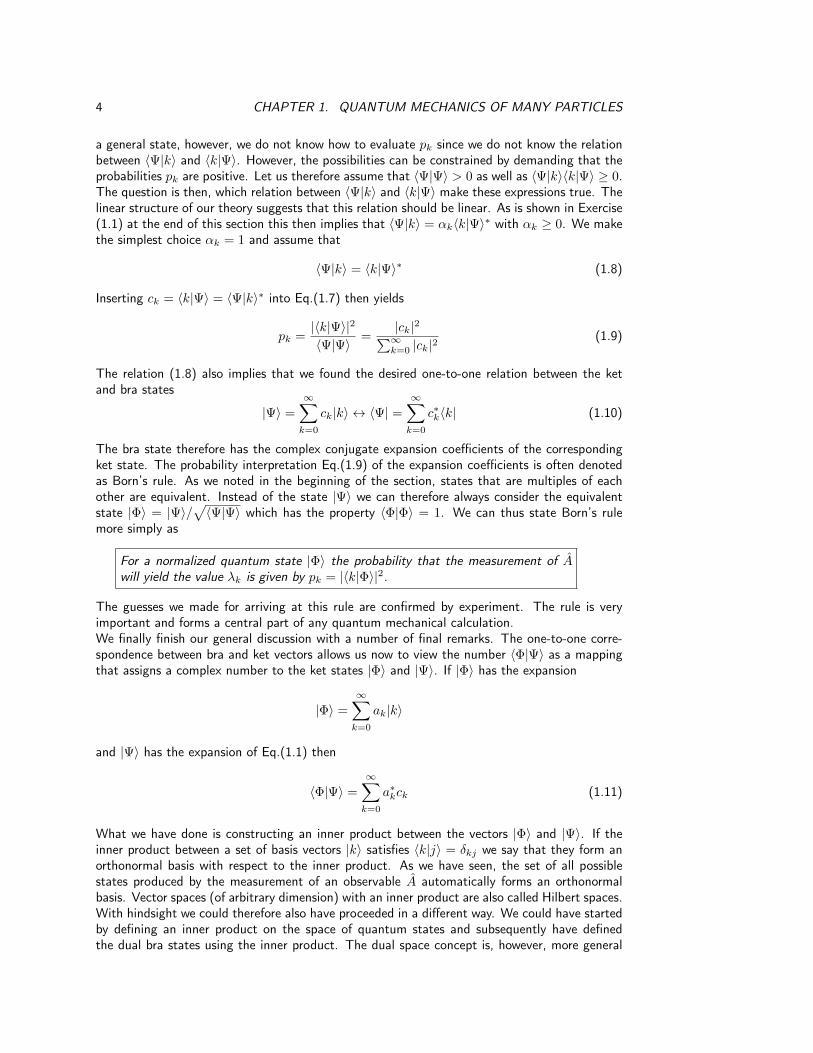
a general state, however, we do not know how to evaluate pk since we do not know the relationbetween 〈Ψ|k〉 and 〈k|Ψ〉. However, the possibilities can be constrained by demanding that theprobabilities pk are positive. Let us therefore assume that 〈Ψ|Ψ〉 > 0 as well as 〈Ψ|k〉〈k|Ψ〉 ≥ 0.The question is then, which relation between 〈Ψ|k〉 and 〈k|Ψ〉 make these expressions true. Thelinear structure of our theory suggests that this relation should be linear. As is shown in Exercise(1.1) at the end of this section this then implies that 〈Ψ|k〉 = αk〈k|Ψ〉∗ with αk ≥ 0. We makethe simplest choice αk = 1 and assume that
〈Ψ|k〉 = 〈k|Ψ〉∗ (1.8)
Inserting ck = 〈k|Ψ〉 = 〈Ψ|k〉∗ into Eq.(1.7) then yields
pk =|〈k|Ψ〉|2
〈Ψ|Ψ〉=
|ck|2∑∞k=0 |ck|2
(1.9)
The relation (1.8) also implies that we found the desired one-to-one relation between the ketand bra states
|Ψ〉 =
∞∑k=0
ck|k〉 ↔ 〈Ψ| =∞∑k=0
c∗k〈k| (1.10)
The bra state therefore has the complex conjugate expansion coefficients of the correspondingket state. The probability interpretation Eq.(1.9) of the expansion coefficients is often denotedas Born’s rule. As we noted in the beginning of the section, states that are multiples of eachother are equivalent. Instead of the state |Ψ〉 we can therefore always consider the equivalentstate |Φ〉 = |Ψ〉/
√〈Ψ|Ψ〉 which has the property 〈Φ|Φ〉 = 1. We can thus state Born’s rule
more simply as
For a normalized quantum state |Φ〉 the probability that the measurement of Awill yield the value λk is given by pk = |〈k|Φ〉|2.
The guesses we made for arriving at this rule are confirmed by experiment. The rule is veryimportant and forms a central part of any quantum mechanical calculation.We finally finish our general discussion with a number of final remarks. The one-to-one corre-spondence between bra and ket vectors allows us now to view the number 〈Φ|Ψ〉 as a mappingthat assigns a complex number to the ket states |Φ〉 and |Ψ〉. If |Φ〉 has the expansion
|Φ〉 =
∞∑k=0
ak|k〉
and |Ψ〉 has the expansion of Eq.(1.1) then
〈Φ|Ψ〉 =
∞∑k=0
a∗kck (1.11)
What we have done is constructing an inner product between the vectors |Φ〉 and |Ψ〉. If theinner product between a set of basis vectors |k〉 satisfies 〈k|j〉 = δkj we say that they form anorthonormal basis with respect to the inner product. As we have seen, the set of all possiblestates produced by the measurement of an observable A automatically forms an orthonormalbasis. Vector spaces (of arbitrary dimension) with an inner product are also called Hilbert spaces.With hindsight we could therefore also have proceeded in a different way. We could have startedby defining an inner product on the space of quantum states and subsequently have definedthe dual bra states using the inner product. The dual space concept is, however, more general

1.1. ONE-PARTICLE QUANTUM MECHANICS 5
and also applies to spaces without inner product. This fact becomes important in the rigorousmathematical formulation of the bra and ket formalism for observables for which the measuredvalues form a continuum.Let us now illustrate our discussion with an explicit example, namely the case of a positionmeasurement in one dimension [4]. We consider a detector that clicks when a particle is withindistance ∆/2 from the position of the detector. We uniformly distribute such detectors on auniform grid with grid points xn = n∆, as to cover the entire one-dimensional world. Let usnow suppose that our one-dimensional world contains a single particle described by a quantumstate |Ψ〉. We now start by carrying a large number N 1 of position measurements. Bycounting the number of times a given detector clicks and dividing the number by N we obtainthe histogram given in Fig.(1.1) which gives the probability for finding the particle in intervaln. According to Born’s rule this probability is given by pn = |〈n|Ψ〉|2, where |n〉 is the statedescribing the particle in the interval xn ±∆/2. The probability to find the particle in |n′〉 justafter the n-th detector has clicked is zero, and hence
〈n|n′〉 = δnn′ . (1.12)
The states |n〉 form a basis for all possible one-particle states. Suppose namely that there wouldbe a state |χ〉 with the property 〈χ|n〉 = 0 for all n. Then this would describe a state wherethe particle is nowhere in our one-dimensional world, contrary to our assumption. The state |Ψ〉can therefore be expanded as
|Ψ〉 =∑n
|n〉〈n|Ψ〉 =∑n
Ψn|n〉 (1.13)
where we defined Ψn = 〈n|Ψ〉. Since Eq.(1.13) is true for all |Ψ〉 we can write
1 =∑n
|n〉〈n|. (1.14)
where 1 is the identity operator that when acting on a ket produces the same ket. This equation isknown as the completeness relation and expresses the fact that the set |n〉 forms an orthonormalbasis. Vice versa, any orthonormal basis satisfies the completeness relation.Let us now assume that we can construct more and more precise detectors and hence reducethe range ∆. Then we can also refine the description of our particle by putting the detectorscloser and closer. In the limit ∆→ 0 the probability |Ψn|2 approaches zero and it makes moresense to reason in terms of the probability density |Ψn|2/∆ of finding the particle in xn. Let usrewrite (1.13) as
|Ψ〉 = ∆∑n
Ψn√∆
|n〉√∆. (1.15)
We now define the continuous function Ψ(xn) and the continuous ket |xn〉 as
Ψ(xn) ≡ lim∆→0
Ψn√∆, |xn〉 = lim
∆→0
|n〉√∆.
In this definition the limiting function Ψ(xn) is well defined while the limiting ket |xn〉 makesmathematical sense only under an integral sign since the norm 〈xn|xn〉 =∞. However, we canstill give to |xn〉 a well precise physical meaning since in quantum mechanics only the “direction”of a ket matters.2 With these definitions (1.15) can be seen as the Riemann sum of Ψ(xn)|xn〉.
2The formulation of quantum mechanics using non-normalizable states requires the extension of Hilbert spacesto rigged Hilbert spaces. Readers interested in the mathematical foundations of this extension can consult, e.g.,Ref. [5]. Here we simply note that in a rigged Hilbert space everything works like in the more familiar Hilbertspace. We simply have to keep in mind that every divergent quantity comes from some continuous limit and thatin all physical quantities the divergency is cancelled by an infinitesimally small quantity.

6 CHAPTER 1. QUANTUM MECHANICS OF MANY PARTICLES
x
|Ψ |2
n
xn
Δ
Figure 1.1: Histogram of the normalized number of clicks of the detector in xn = n∆. Theheight of the function corresponds to the probability |Ψn|2.
In the limit ∆→ 0 the sum becomes an integral over x and we can write
|Ψ〉 =
∫dx|x〉〈x|Ψ〉 =
∫dx Ψ(x)|x〉. (1.16)
The function Ψ(x) is usually called the wavefunction or the probability amplitude and its squaremodulus |Ψ(x)|2 is the probability density of finding the particle in x, or equivalently
|Ψ(x)|2 dx =
(probability of finding the particlein volume element dx around x
).
In the continuum formulation the orthonormality relation (1.12) becomes
〈x|x′〉 = δ(x− x′),
where δ(x) is the Dirac δ-function with the property
f(x) =
∫dx′f(x′)δ(x− x′)
Indeed, if we act with 〈x| on |Ψ〉 we see from Eq.(1.16) that
〈x|Ψ〉 =
∫dx′Ψ(x′)〈x|x′〉 =
∫dx′Ψ(x′)δ(x− x′) = Ψ(x) (1.17)
For the continuum case the completeness relation (1.14) becomes∫dx |x〉〈x| = 1.
Using this relation we can write the innner product between states |Ψ〉 and |Φ〉 as
〈Φ|Ψ〉 =
∫dx 〈Φ|x〉〈x|Ψ〉 =
∫dxΦ∗(x)Ψ(x)
This is how the inner product is usually introduced in elementary quantum mechanics courses.Mathematically the inner product is well-defined for so-called quadratically integrable functions,i.e. functions for which the integral of |Ψ(x)|2 is finite. The wave function Ψ(x) often plays

1.1. ONE-PARTICLE QUANTUM MECHANICS 7
a central role in elementary introductions to quantum mechanics. We see from our discussion,however, that Ψ(x) is only the projection of the quantum state |Ψ〉 on the position basis |x〉.The more fundamental object is therefore the state |Ψ〉. We could have prepared our systemin the same quantum state |Ψ〉 but carried out momentum measurements instead. In that casethe expansion coefficients of interest would have been Ψ(p) = 〈p|Ψ〉 where |p〉 are momentumstates. This would amount to expanding the same state |Ψ〉 in a different basis. The bra andket formalism invented by Dirac highlights the vector space structure of quantum mechanicsindependent of the basis that is used.
Exercise 1.1 Let a and b be complex numbers and let b depend on a in such a way that alwaysab is real and ab ≥ 0. Show that when a 6= 0 the most general form the function b(a) can haveis b(a) = f(a)a∗ where f(a) is an arbitrary function of a with the property that f(a) is real andf(a) ≥ 0 (for a = 0 we can obviously choose b to be whatever we want). Show further that if bis a linear function in the sense that b(λa) = λb(a) for a real number λ, then the only possibilityis b(a) = αa∗ with α real and α ≥ 0.
1.1.2 Observables and linear operators
Until now we only considered the vector structure of the set of quantum states. However, todo physics we have to give rules on how the quantum states change when we study physicalprocesses. Since a physical process quantum states into new states we will associate with variousphysical quantities (which we call observables) that play a role in the physical process an operatorA that acts on states and produces new states, i.e.
|χ〉 = A|Φ〉 (1.18)
Since we have the superposition principle we assume that the operator A is linear and therefore
A(c1|Ψ1〉+ c2|Ψ2〉) = c1A|Ψ1〉+ c2A|Ψ2〉 (1.19)
Similarly we can define linear operators on the bra states. Let is fix a bra state 〈Φ| and anoperator A acting on ket states. Then there is a unique bra state 〈χ| that has the property that
〈χ|Ψ〉 = 〈Φ|A|Ψ〉 (1.20)
for all possible ket states |Ψ〉. We will denote this state by 〈χ| = 〈Φ|A, which defines the actionof A on the bra state 〈Φ|. An operator can therefore act both on bra and ket states. The states|χ〉 and |Φ〉 of Eq.(1.18) have dual bra states 〈Φ| and 〈χ|. We can ask ourselves, which operatorconnects these two bra states. We call the corresponding operator A†, also known as the adjointof A. Then we have
|χ〉 = A|Φ〉 ↔ 〈χ| = 〈Φ|A† (1.21)
If we act on the state |Ψ〉 and on the dual state 〈Ψ| using the right and left side of thiscorrespondence we obtain the equations
〈Ψ|A|Φ〉 = 〈Ψ|χ〉 = 〈χ|Ψ〉∗ = 〈Φ|A†|Ψ〉∗ (1.22)
for all possible states |Φ〉 and |Ψ〉. This completely defines the matrix elements of A† in termsof those of A, and hence the operator. Let |k〉 namely be an orthonormal basis then from thecompleteness relation we see that
A =∑i,j
|i〉〈i|A|j〉〈j| =∑i,j
Aij |i〉〈j|

8 CHAPTER 1. QUANTUM MECHANICS OF MANY PARTICLES
The adjoint operator therefore has the expansion
A† =∑i,j
|i〉〈i|A†|j〉〈j| =∑i,j
A∗ji|i〉〈j|
Let us now go back to the discussion of quantum measurements. If we prepare a system in astate |Ψ〉 and measure observable A we obtain with probability pk a state |k〉 corresponding toa quantum state in which the physical quantity (energy, spin, momentum, position, etc.) hasa sharply defined value λk. The measurement itself can not be described by the action of Aon |Ψ〉 since we do not have a definite outcome, but we can only speak of the probability pkof a certain outcome. However, if we prepare the system in state |k〉 the measurement of Amust leave the state intact, and we can predict the outcome with certainty. We describe thismathematically by requiring that
A|k〉 = µk|k〉 (1.23)
where µk is a proportionality constant. The proportionality constant is not unity, otherwise theoperator A would simply be the unit operator (remember that the state |k〉 form a completeset). Since A represents a physical observable the constants µk must be related to the physicaloutcomes λk of the measurement. Again, due to the linear structure of the space of quantumstates we assume this relation to be linear and we make the simple choice µk = λk. We thenhave
A|k〉 = λk|k〉 (1.24)
This is mathematically an eigenvalue equation, and we therefore say that |k〉 is an eigenstate ofoperator A with eigenvalue λk. From the eigenvalue equation it follows that we can representA as
A =
∞∑k=0
λk|k〉〈k| (1.25)
as can be checked by acting on a basis vector |j〉 using the orthonormality of the state |k〉. Aphysical observable is therefore completely determined by its set of physical measurable outcomes.This is indeed what one would like to demand of an observable. If the set of eigenvalues of anoperator is discrete we say that the operator has a discrete spectrum, and when it is continuouswe say that it has a continuous spectrum. The most general operator has both a discrete andcontinuous spectrum.
Now consider an arbitrary normalized quantum state |Ψ〉 that is expressed as in Eq.(1.1) interms of the states |k〉. When we measure the observable A we obtain the outcome λk withprobability pk = |ck|2. If we repeat the experiment many times then the average value wemeasure is called the expectation value 〈A〉 of A and given by
〈A〉 =
∞∑k=0
λk |ck|2 =
∞∑k=0
〈Ψ|k〉λk〈k|Ψ〉 = 〈Ψ|A|Ψ〉 (1.26)
where in the last step we used the form Eq.(1.25) of the expansion of the operator A. This valueis called the expectation value of the operator A. The average of our measurement should bea real number. One may object that complex numbers could also be allowed since the real andimaginary parts could separately correspond to measured values. However, this would requiretwo measurements and as we shall see, in general the measurement of two quantities on the samestate (such as, for example, position and momentum) is not possible in quantum mechanics.We therefore require that 〈Ψ|A|Ψ〉 is a real number, i.e., we demand that
Im〈Ψ|A|Ψ〉 = 0 (1.27)

1.1. ONE-PARTICLE QUANTUM MECHANICS 9
for all possible states |Ψ〉. This is, in particular, true for a state of the form |Ψ〉 = |Φ〉+ λ|χ〉,for all possible choices of |Φ〉, |χ〉 and λ. From this it follows (see Exercise) that
〈Φ|A|χ〉 = 〈χ|A|Φ〉∗ (1.28)
for all possible states |Φ〉 and |χ〉. Operators with this property are called Hermitian operators.By comparing to Eq.(1.22) we see that Hermitian operators have the property that A = A† andare therefore equal to their adjoint operators. An important property of Hermitian operators isthat their eigenvalues are always real and that their eigenstates with different eigenvalues areorthogonal. This is readily shown. Let |k〉 denote the eigenstates, then
0 = 〈j|A|k〉 − 〈k|A|j〉∗ = λk〈j|k〉 − λ∗j 〈j|k〉∗ = (λk − λ∗j )〈j|k〉
Therefore, if j = k we find (since 〈k|k〉 6= 0) that λk = λ∗k and hence all eigenvalues are real.But then 0 = (λk − λj)〈j|k〉 and we find that if λj 6= λk that 〈j|k〉 = 0. In case that there aremore states with the same eigenvalue, this subset of states can always made into an orthogonalset and by normalization into an orthonormal set. The Hermitian operator has, therefore exactlythe property that we want from it. Let us now consider the case that we want to measure twoobservables A and B on a quantum state. This will be possible whenever the operators A andB commute, i.e. when [
A, B]≡ AB − BA = 0 (1.29)
The reason is that commuting operators have a common set of eigenstates. This is readilyshown. Let us denote the eigenvalues of operator A by λa. In general this eigenvalue could bedegenerate, i.e. there could be several linearly independent eigenstates |a, 1〉, . . . , |a,m〉 (withm arbitrary) with the same eigenvalue λa. The space spanned by these degenerate eigenvectorswill be denoted by Va. Let |v〉 be an arbitrary state in Va then
AB|v〉 = BA|v〉 = λaB|v〉
This means that B|v〉 ∈ Va. Therefore the operator B maps vectors from Va to vectors in Va.We can therefore diagonalize the operator B in this subspace and find m eigenstates of B thatall have eigenvalue λa for operator A. This shows that we can find a common set of eigenstateof A and B.
1.1.3 Quantum dynamics and the Schrödinger equation
So far, we described quantum states and observables, but we did not derive any dynamical lawsfor them. In a dynamical process the quantum states move in time. This corresponds in Hilbertspace with a vector |Ψ(t)〉 which a direction that changes with the time t. Suppose we considera vector at time t0, given by |Ψ(t0)〉, then we can define the evolution operator U(t, t0) thatmaps the initial ket vector to the ket at another time t, i.e.
|Ψ(t)〉 = U(t, t0)|Ψ(t0)〉
In order to preserve the probability interpretation for all times we must demand that the time-dependent states remain normalized, i.e.
〈Ψ(t0)|Ψ(t0)〉 = 〈Ψ(t)|Ψ(t)〉 = 〈Ψ(t0)|U†(t, t0)U(t, t0)|Ψ(t0)〉
This must be true for arbitrary initial states |Ψ(t0)〉. In the Exercise you are asked to prove thatif 〈Ψ|O|Ψ〉 = 〈Ψ|Ψ〉 for arbitrary states |Ψ〉 then O = 1 is equal to the unit operator. We thusfind that
U†(t, t0)U(t, t0) = 1 (1.30)
10 CHAPTER 1. QUANTUM MECHANICS OF MANY PARTICLES
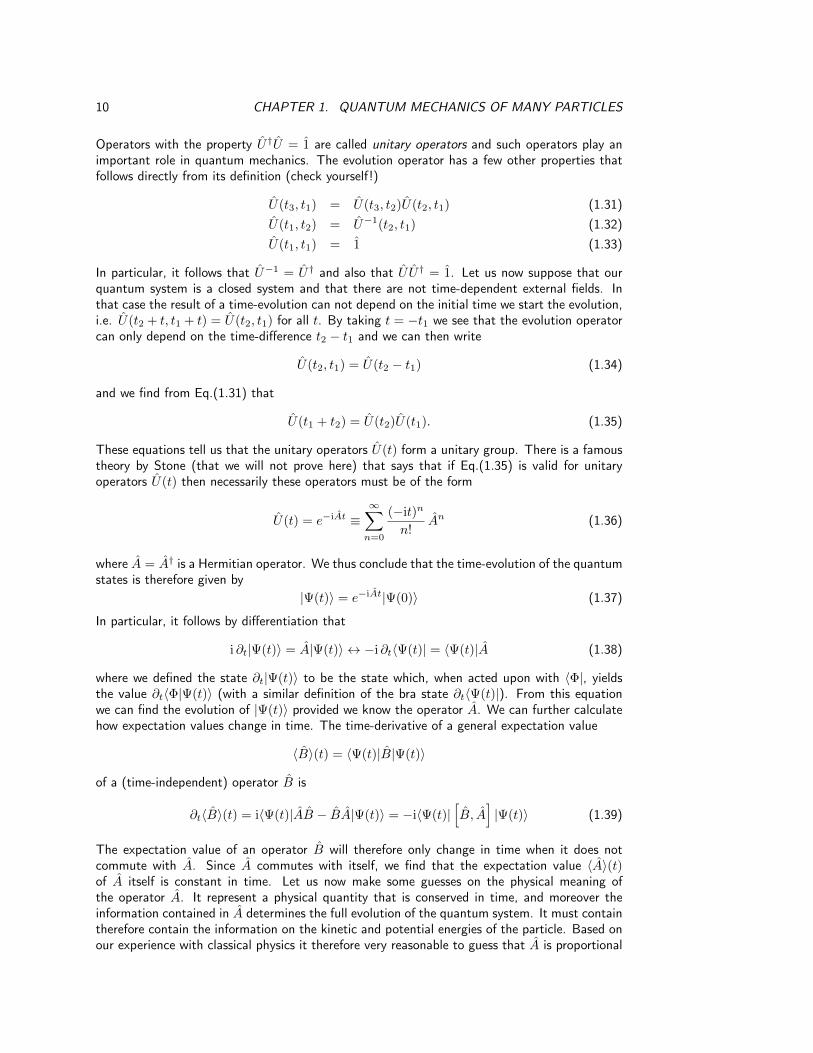
Operators with the property U†U = 1 are called unitary operators and such operators play animportant role in quantum mechanics. The evolution operator has a few other properties thatfollows directly from its definition (check yourself!)
U(t3, t1) = U(t3, t2)U(t2, t1) (1.31)U(t1, t2) = U−1(t2, t1) (1.32)U(t1, t1) = 1 (1.33)
In particular, it follows that U−1 = U† and also that U U† = 1. Let us now suppose that ourquantum system is a closed system and that there are not time-dependent external fields. Inthat case the result of a time-evolution can not depend on the initial time we start the evolution,i.e. U(t2 + t, t1 + t) = U(t2, t1) for all t. By taking t = −t1 we see that the evolution operatorcan only depend on the time-difference t2 − t1 and we can then write
U(t2, t1) = U(t2 − t1) (1.34)
and we find from Eq.(1.31) that
U(t1 + t2) = U(t2)U(t1). (1.35)
These equations tell us that the unitary operators U(t) form a unitary group. There is a famoustheory by Stone (that we will not prove here) that says that if Eq.(1.35) is valid for unitaryoperators U(t) then necessarily these operators must be of the form
U(t) = e−iAt ≡∞∑n=0
(−it)n
n!An (1.36)
where A = A† is a Hermitian operator. We thus conclude that the time-evolution of the quantumstates is therefore given by
|Ψ(t)〉 = e−iAt|Ψ(0)〉 (1.37)
In particular, it follows by differentiation that
i ∂t|Ψ(t)〉 = A|Ψ(t)〉 ↔ −i ∂t〈Ψ(t)| = 〈Ψ(t)|A (1.38)
where we defined the state ∂t|Ψ(t)〉 to be the state which, when acted upon with 〈Φ|, yieldsthe value ∂t〈Φ|Ψ(t)〉 (with a similar definition of the bra state ∂t〈Ψ(t)|). From this equationwe can find the evolution of |Ψ(t)〉 provided we know the operator A. We can further calculatehow expectation values change in time. The time-derivative of a general expectation value
〈B〉(t) = 〈Ψ(t)|B|Ψ(t)〉
of a (time-independent) operator B is
∂t〈B〉(t) = i〈Ψ(t)|AB − BA|Ψ(t)〉 = −i〈Ψ(t)|[B, A
]|Ψ(t)〉 (1.39)
The expectation value of an operator B will therefore only change in time when it does notcommute with A. Since A commutes with itself, we find that the expectation value 〈A〉(t)of A itself is constant in time. Let us now make some guesses on the physical meaning ofthe operator A. It represent a physical quantity that is conserved in time, and moreover theinformation contained in A determines the full evolution of the quantum system. It must containtherefore contain the information on the kinetic and potential energies of the particle. Based onour experience with classical physics it therefore very reasonable to guess that A is proportional
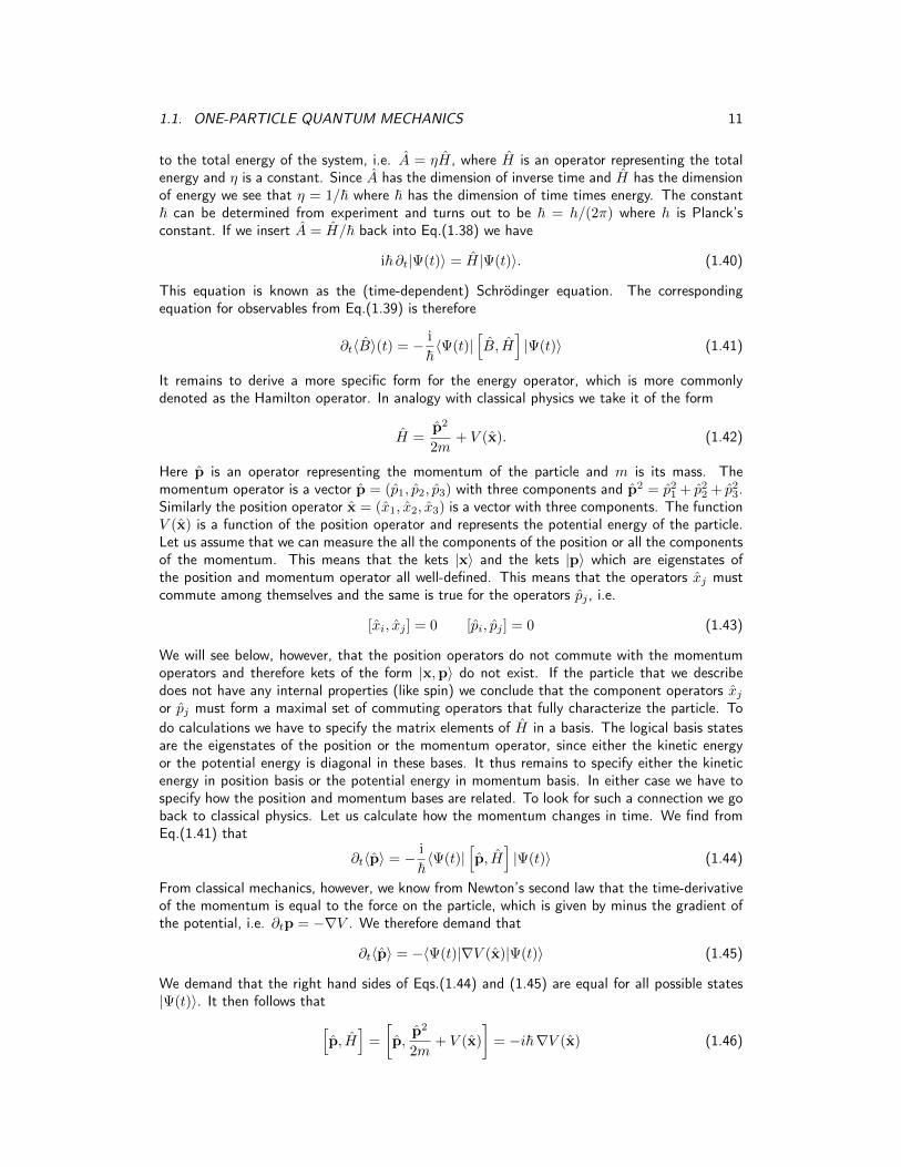
1.1. ONE-PARTICLE QUANTUM MECHANICS 11
to the total energy of the system, i.e. A = ηH, where H is an operator representing the totalenergy and η is a constant. Since A has the dimension of inverse time and H has the dimensionof energy we see that η = 1/~ where ~ has the dimension of time times energy. The constant~ can be determined from experiment and turns out to be ~ = h/(2π) where h is Planck’sconstant. If we insert A = H/~ back into Eq.(1.38) we have
i~ ∂t|Ψ(t)〉 = H|Ψ(t)〉. (1.40)
This equation is known as the (time-dependent) Schrödinger equation. The correspondingequation for observables from Eq.(1.39) is therefore
∂t〈B〉(t) = − i
~〈Ψ(t)|
[B, H
]|Ψ(t)〉 (1.41)
It remains to derive a more specific form for the energy operator, which is more commonlydenoted as the Hamilton operator. In analogy with classical physics we take it of the form
H =p2
2m+ V (x). (1.42)
Here p is an operator representing the momentum of the particle and m is its mass. Themomentum operator is a vector p = (p1, p2, p3) with three components and p2 = p2
1 + p22 + p2
3.Similarly the position operator x = (x1, x2, x3) is a vector with three components. The functionV (x) is a function of the position operator and represents the potential energy of the particle.Let us assume that we can measure the all the components of the position or all the componentsof the momentum. This means that the kets |x〉 and the kets |p〉 which are eigenstates ofthe position and momentum operator all well-defined. This means that the operators xj mustcommute among themselves and the same is true for the operators pj , i.e.
[xi, xj ] = 0 [pi, pj ] = 0 (1.43)
We will see below, however, that the position operators do not commute with the momentumoperators and therefore kets of the form |x,p〉 do not exist. If the particle that we describedoes not have any internal properties (like spin) we conclude that the component operators xjor pj must form a maximal set of commuting operators that fully characterize the particle. Todo calculations we have to specify the matrix elements of H in a basis. The logical basis statesare the eigenstates of the position or the momentum operator, since either the kinetic energyor the potential energy is diagonal in these bases. It thus remains to specify either the kineticenergy in position basis or the potential energy in momentum basis. In either case we have tospecify how the position and momentum bases are related. To look for such a connection we goback to classical physics. Let us calculate how the momentum changes in time. We find fromEq.(1.41) that
∂t〈p〉 = − i
~〈Ψ(t)|
[p, H
]|Ψ(t)〉 (1.44)
From classical mechanics, however, we know from Newton’s second law that the time-derivativeof the momentum is equal to the force on the particle, which is given by minus the gradient ofthe potential, i.e. ∂tp = −∇V . We therefore demand that
∂t〈p〉 = −〈Ψ(t)|∇V (x)|Ψ(t)〉 (1.45)
We demand that the right hand sides of Eqs.(1.44) and (1.45) are equal for all possible states|Ψ(t)〉. It then follows that[
p, H]
=
[p,
p2
2m+ V (x)
]= −i~∇V (x) (1.46)

12 CHAPTER 1. QUANTUM MECHANICS OF MANY PARTICLES
Since this equation is valid for any potential V it is also valid for V = 0, and we see that[p,
p2
2m
]= 0.
From this we see that Eq.(1.46) becomes
[p, V (x)] = −i~∇V (x) (1.47)
This is the basic relation between the position and momentum operators that we have beenlooking for. In the special case that we take V (x) = xi this yields the relations
[xi, pj ] = i~ δij (1.48)
These commutation relations show that we cannot simultaneously determine both the positionand the momentum of a particle since we can not find a common eigenbasis. Let us nowevaluate expression (1.47) in the position basis. Using the orthonormality of the basis kets〈x|x′〉 = δ(x− x′) and x|x〉 = x|x〉 we find
−i~∇V (x)δ(x− x′) = 〈x|pV (x)− V (x)p|x′〉 = 〈x|p|x′〉V (x′)− V (x)〈x|p|x′〉 (1.49)
From this expression we can readily guess a possible solution. For instance,
〈x|p|x′〉 = −i~∇δ(x− x′) (1.50)
is a solution. If we insert (1.50) into (1.49) and integrate with a test function f(x′) over thecoordinates x′ we find
−i~ (∇V (x))f(x) = −i~∇(V (x)f(x)) + i~V (x)∇f(x) (1.51)
which is clearly an identity for any test function. We therefore found a solution, but is this themost general solution to Eq.(1.49)? We can, without loss of generality, write
〈x|p|x′〉 = −i~∇δ(x− x′) + 〈x|f |x′〉 (1.52)
where f is a vector operator to be determined. Inserting this expression back into (1.49) thenyields the expression
0 = 〈x|f |x′〉V (x′)− V (x)〈x|f |x′〉 = 〈x|[f , V (x)
]|x′〉
or equivalently0 =
[f , V (x)
](1.53)
We find that f commutes with any function of the position operator. In particular it thencommutes with the operators xj . Since operators xj form a maximal commuting set the operatorf must be a function of the position operator f = f(x). This means, using Eq.(1.54), that themost general form of the momentum operator is
〈x|p|x′〉 = −i~∇δ(x− x′) + f(x)δ(x− x′). (1.54)
The components of the vector fj(x) are, however, not independent. From the relations [pi, pj ] =0 we can prove (see Exercise) that
∂fi∂xj− ∂fj∂xi
= 0

1.1. ONE-PARTICLE QUANTUM MECHANICS 13
and we see that the curl of the vector field f vanishes. This implies that f must be the gradientof a scalar function f = ∇F (x) and that
〈x|p|x′〉 = −i~∇δ(x− x′) + δ(x− x′)∇F (x). (1.55)
If we multiply both sides with Ψ(x′) = 〈x′|Ψ〉 and integrate over x′ we can write this equivalentlyas
〈x|p|Ψ〉 =
∫dx′ 〈x|p|x′〉〈x′|Ψ〉 = −i~∇Ψ(x) + Ψ(x)∇F (x). (1.56)
We will now show that we can always choose a new position basis such that the function F inEq.(1.55) vanishes. To do this we make use of the fact that normalized kets are defined only upto a phase factor. We can defined new position ket states defined by
|x〉 ≡ e− i~F (x)|x〉 (1.57)
These are still eigenstates of the position operator x|x〉 = x|x〉 and properly normalized, i.e.〈x|x′〉 = δ(x− x′). Let us express the matrix elements of p in the new basis. Using Eq. (1.55)we have
〈x|p|x′〉 = ei~F (x)〈x|p|x′〉e− i
~F (x′)
= −i~ ei~F (x)∇δ(x− x′)e−
i~F (x′) + δ(x− x′)∇F (x)
= −i~∇δ(x− x′) (1.58)
The identity between the last two lines follows again by integrating against a test function g(x′),which gives the true identity
−i~ ei~F (x)∇(g(x)e−
i~F (x)) + g(x)∇F (x) = −i~∇g(x).
We thus see that we can always choose a basis in which the momentum operator has thematrix elements as in Eq.(1.58). This is called the Schrödinger representation of the momentumoperator. In the following we will always choose this basis and denote the corresponding positionbasis elements again by |x〉. Then, as in Eq.(1.56), we obtain the important expression
〈x|p|Ψ〉 = −i~∇〈x|Ψ〉. (1.59)
Let us now go back to the Schrödinger equation (1.40) which we write more explicitly as
i~ ∂t|Ψ(t)〉 =
(p2
2m+ V (x)
)|Ψ(t)〉. (1.60)
Since we now explicitly now the matrix elements of the operators in the position basis we canfind an explicit evolution equation for the quantum state |Ψ(t)〉. Let denote it representation inposition basis as Ψ(x, t) = 〈x|Ψ(t)〉. Acting with the bra states 〈x| on both sides of Eq.(1.60)gives
i~ ∂tΨ(x, t) =1
2m〈x|p2|Ψ(t)〉+ 〈x|V (x)|Ψ(t)〉 (1.61)
Since V (x) is a function of the position operator the last term on the right hand side is simply〈x|V (x)|Ψ(t)〉 = V (x)Ψ(x, t) and we only need to work out the first term. This gives
〈x|p2|Ψ(t)〉 =
3∑j=1
∫dx′ 〈x|pj |x′〉〈x′|pj |Ψ(t)〉
= (−i~)23∑j=1
∫dx′ ∂jδ(x− x′)∂jΨ(x′, t) = −~2
3∑j=1
∂2jΨ(x, t)
= −~2∇2Ψ(x, t) (1.62)

14 CHAPTER 1. QUANTUM MECHANICS OF MANY PARTICLES
This means that in position basis the Schrödinger equation attains the form
i~ ∂tΨ(x, t) =
(− ~2
2m∇2 + V (x)
)Ψ(x, t) (1.63)
This is the way the Schrödinger equation was originally presented. Let us finally see how thingslook like in the momentum basis. The momentum basis is defined by |p〉 and defined by theeigenvalue equation p|p〉 = p|p〉. If we therefore take the state |Ψ〉 in Eq.(1.59) to be equal to|p〉 we find
p〈x|p〉 = −i~∇〈x|p〉 (1.64)
This is a differential equation for the matrix element ∇〈x|p〉 with the solution
〈x|p〉 = C ei~p·x (1.65)
1.1.4 Rotations and electron spin
The concept of electron spin is closely related to the transformation properties of quantum statesunder rotations. Let us therefore start with a discussion of rotations in 3-dimensional space. Letus start by simply considering the rotations around the coordinate axes. These are described bythe matrices
Rz(θ) =
cos θ − sin θ 0sin θ cos θ 0
0 0 1
(1.66)
Rx(φ) =
1 0 00 cosφ − sinφ0 sinφ cosφ
(1.67)
Ry(ψ) =
cosψ 0 sinψ0 1 0
− sinψ 0 cosψ
(1.68)
which rotate a 3-dimensional vector over angles θ, φ and ψ around the z, x and y-axes. Letus consider, for instance, the rotations Rz(θ) around the z-axis. It is clear that this rotationsatisfies
Rz(θ) = Rz(θ
N)N . (1.69)
In other words, a rotation over angle θ can be performed by subsequently rotation N times oversmaller angle θ/N . If we take N large enough then θ/N 1 and we can write
Rz(θ
N) ≈ 1 +
θ
N
dRz
dθ|θ=0 + . . . = 1− i
θ
NLz + . . . (1.70)
where we defined
Lz = idRz
dθ|θ=0 =
0 −i 0i 0 00 0 0
(1.71)
Then we can write Eq.(1.69) as
Rz(θ) = limN→∞
Rz(θ
N)N = lim
N→∞(1− i
θ
NLz)
N = e−iθLz (1.72)
where we used the well-known identity
ex = limN→∞
(1 +x
N)N .

1.1. ONE-PARTICLE QUANTUM MECHANICS 15
It is readily checked that the expansion
e−iθLz =
∞∑n=0
(−iθLz)n
n!(1.73)
indeed gives back Eq.(1.66). Check this for yourself: just work out the powers of Lz and usethe Taylor expansions for the sine an cosine functions. We similarly find
Rx(φ) = e−iφLx Ry(ψ) = e−iψLy (1.74)
where we defined
Lx = idRx
dφ|φ=0 =
0 0 00 0 −i0 i 0
(1.75)
Ly = idRy
dψ|ψ=0 =
0 0 i0 0 0−i 0 0
(1.76)
The matrices Lx, Ly and Lz are often called the generators of infinitesimal rotations. It is readilyverified that these matrices satisfy the commutation relations
[Lx, Ly] = iLz [Ly, Lz] = iLx [Lz, Lx] = iLy (1.77)
Rather than rotations along the coordinate axes we can also consider a rotation around anarbitrary vector. Let us denote this vector by n and let us take this vector to have lenght one,i.e. |n| = 1. A rotation of a vector r around n over a small angle ∆φ gives
Rn(∆φ)r ≈ r + ∆φn× r + . . . (1.78)
This is derived by noting that first order change is orthogonal to n and r and has the length∆φ|n × r| = ∆φ| sin(∠(n, r))|. If we write out r = (x1, x2, x3) and n = (n1, n2, n3) incomponents we can write
n× r =
n2x3 − n3x2
n3x1 − n1x3
n1x2 − n2x1
=
0 −n3 n2
n3 0 −n1
−n2 n1 0
r.
We thus find that
Rn(∆φ) = 1 + ∆φ
0 −n3 n2
n3 0 −n1
−n2 n1 0
+ . . .
= 1− i∆φ(n1Lx + n2Ly + n3Lz) + . . . (1.79)
With then find that a rotation with an angle φ around an axis n is given by
Rn(φ) = limN→∞
Rn(φ
N)N = lim
N→∞(1− i
φ
Nn · L)N = e−iφn·L (1.80)
where we defined the vector of matrices L = (Lx, Ly, Lz). Now that we discussed rotationswe go back to quantum mechanics and ask ourselves how a rotation in physical space (likethe rotation of a magnet in the Stern-Gerlach experiment) affects the quantum states that wemeasure. We therefore have to make a connection between rotations in real space and the

16 CHAPTER 1. QUANTUM MECHANICS OF MANY PARTICLES
rotations in Hilbert space. We therefore assign to every rotation Rn(φ) in real space an operatorUn(φ) that rotates kets, i.e.
|ΨR〉 = Un(φ)|Ψ〉 ↔ 〈ΨR| = 〈Ψ|U†n(φ) (1.81)
where |ΨR〉 stands for the rotated ket. Since rotations should not change the norm of the stateswe must have that
〈Ψ|Ψ〉 = 〈Ψ|U†n(φ)Un(φ)|Ψ〉 (1.82)
for all possible ket states |Ψ〉. This implies that U†n(φ)Un(φ) = 1 and hence U†n(φ) = U−1n (φ) =
Un(−φ). Furthermore the operators Un(φ) must have the same product properties as that ofthe rotation matrices. We therefore have the correspondence
Rn(φ1 + φ2) = Rn(φ2)Rn(φ1)↔ Un(φ1 + φ2) = Un(φ2)Un(φ1) (1.83)
Such a correspondence between operators on two different vector spaces is called a representation.The group of rotations in three dimensions induces a representation on the infinite dimensionalHilbert space of quantum states. To define an operator we have to specify it in a basis, and theposition basis |r〉 is an obvious choice. We define
Un(φ)|r〉 ≡ |Rn(φ)r〉. (1.84)
This is clearly a natural definition; the rotated position ket is simply the ket for the rotatedposition. We find therefore that for the bra states
〈Rn(φ)r| = 〈r|U†n(φ) = 〈r|Un(−φ). (1.85)
Let us now look the a general rotated quantum state Un(φ)|Ψ〉. From Eq.(1.85) it follows thatthe rotated state in position basis is given by
〈r|Un(φ)|Ψ〉 = 〈Rn(−φ)r|Ψ〉 = Ψ(Rn(−φ)r) (1.86)
Let us now evaluate the last term for a small angle ∆φ. We then have that
〈r|Un(∆φ)|Ψ〉 = Ψ(Rn(−∆φ)r) = Ψ(r−∆φn× r + . . . )
= Ψ(r)−∆φ (n× r) · ∇Ψ(r) + . . . =
(1− i
~∆φn · (−i~ r×∇) + . . .
)Ψ(r)
= 〈r|1− i
~∆φn · L + . . . |Ψ〉 (1.87)
where we defined the angular momentum operator L by
〈r|L|Ψ〉 = 〈r|r× p|Ψ〉 = −i~ r×∇〈r|Ψ〉 (1.88)
As before we can now calculate
〈r|Un(φ)|Ψ〉 = limN→∞
〈r|(Un(φ
N))N |Ψ〉
= limN→∞
〈r|(1− i
~φ
Nn · L)N |Ψ〉 = 〈r|e− i
~ φn·L|Ψ〉 (1.89)
We therefore find that the operator Un(φ) has the form
Un(φ) = e−i~ φn·L. (1.90)

1.1. ONE-PARTICLE QUANTUM MECHANICS 17
It has the same form as rotation operator Rn(φ) of Eq.(1.80) but now the exponent containsthe vector operator L that acts in Hilbert space rather than than a vector of 3× 3-matrices. Itfollows directly from the commutation relations of the position and momentum operators (checkyourself!) that the components Lx, Ly and Lx of the angular momentum operator satisfy thesame relations as those of the generators of the infinitesimal rotations Eq.(1.77), i.e.
[Lx, Ly] = i~ Lz [Ly, Lz] = i~ Lx [Lz, Lx] = i~ Ly. (1.91)
Now we have enough background to introduce the concept of spin. We have found that thereexists a representation of the rotation group on an infinite-dimensional Hilbert space. Next weask ourselves the question whether we can find a representation on other vector spaces. Thereason is that we want to add to the point particles that we have been considering internalproperties. These internal properties are described by a finite-dimensional space, which meansthat the quantum states of a particle can be described by a finite vector of kets. These kets canbe transformed among each other by rotations. This will become more clear when we proceed.The smallest non-trivial vector space that we can consider is the two-dimensional space, andthis turns out to be exactly the vector space we need. From the previous discussion it is nowclear how to find a two-dimensional presentation. We need to find 2× 2-matrices satisfying therelations (1.77) and then take the exponent as in Eq.(1.80). The matrices that we need aregiven by the Pauli-matrices
σ =
(0 11 0
)σy =
(0 −ii 0
)σz =
(1 00 −1
)(1.92)
It is readily checked that the matrices σi/2 (i = x, y, z) satisfy the required commutationrelations, i.e.
[σx
2,σy
2] = i
σz
2[σy
2,σz
2] = i
σx
2[σz
2,σx
2] = i
σy
2(1.93)
We can now, in analogy, to Eq.(1.80) construct the 2× 2-matrix
Un(φ) = e−i2 φn·σ (1.94)
where σ = (σx, σy, σz) is a vector of matrices. The matrix Un(φ) induces a rotation in ourtwo-dimensional space. We have now succeeded in defining the required rotation matrix in twodimensions, but one may wonder whether our procedure is unique. Could there not be a set ofthree different 2× 2-matrices σj that satisfy the same commutation relations as in Eq.(1.93) ?One can show that the only possibility for this is
σj = V †σjV (1.95)
for an arbitrary unitary 2 × 2-matrix V , i.e. satisfying V †V = 1 (Check for yourself that thispreserves the commutation relations). However, such a transformation simply amounts to a basischange in the two-dimensional space that we consider and we can therefore always choose a basisin which the Pauli matrices have the form of Eq.(1.92). In this basis the vectors e1 = (1, 0)and e2 = (0, 1) are invariant under rotations around the z-axis (of the original three-dimensionalspace), i.e. if we take n = (0, 0, 1) then
Un(φ) = e−i2 φn·σ = e−
i2 φσz =
(e−
i2φ 0
0 ei2φ
), (1.96)
which maps e1 and e2 to multiples of themselves. If we had used the alternative representationof Eq.(1.95) this would have been true for the vectors V †e1 and V †e2 instead.Let us now find a more explicit form for the matrix of Eq.(1.94). To do this we first derive a
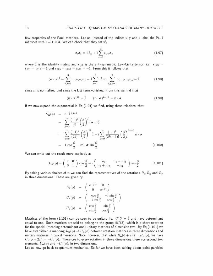
18 CHAPTER 1. QUANTUM MECHANICS OF MANY PARTICLES
few properties of the Pauli matrices. Let us, instead of the indices x, y and z label the Paulimatrices with i = 1, 2, 3. We can check that they satisfy
σiσj = 1 δij + i
3∑k=1
εijkσk (1.97)
where 1 is the identity matrix and εijk is the anti-symmetric Levi-Civita tensor, i.e. ε123 =ε231 = ε312 = 1 and ε213 = ε132 = ε321 = −1. From this it follows that
(n · σ)2 =
3∑i,j=1
ninjσiσj = 1
3∑i=1
n2i + i
2∑i,j,k=1
ninjεijkσk = 1 (1.98)
since n is normalized and since the last term vanishes. From this we find that
(n · σ)2k = 1 (n · σ)2k+1 = n · σ (1.99)
If we now expand the exponential in Eq.(1.94) we find, using these relations, that
Un(φ) = e−i2 φn·σ
=
∞∑j=0
(−i)j
j!
(φ
2
)j(n · σ)j
=
∞∑k=0
(−1)k
(2k)!
(φ
2
)2k
1− i
∞∑k=0
(−1)k
(2k + 1)!
(φ
2
)2k+1
n · σ
= 1 cosφ
2− i n · σ sin
φ
2. (1.100)
We can write out the result more explicitly as
Un(φ) =
(1 00 1
)cos
φ
2− i
(n3 n1 − in2
n1 + in2 −n3
)sin
φ
2(1.101)
By taking various choices of n we can find the representatives of the rotations Rz, Rx and Ryin three dimensions. These are given by
Uz(φ) =
(e−
i2φ 0
0 ei2φ
)Ux(φ) =
(cos φ2 −i sin φ
2
−i sin φ2 cos φ2
)Uy(φ) =
(cos φ2 − sin φ
2
sin φ2 cos φ2
)Matrices of the form (1.101) can be seen to be unitary i.e. U†U = 1 and have determinantequal to one. Such matrices are said to belong to the group SU(2), which is a short notationfor the special (meaning determinant one) unitary matrices of dimension two. By Eq.(1.101) wehave established a mapping Rn(φ)→ Un(φ) between rotation matrices in three dimensions andunitary matrices in two dimensions. Note, however, that while Rn(φ + 2π) = Rn(φ), we haveUn(φ + 2π) = −Un(φ). Therefore to every rotation in three dimensions there correspond twoelements, Un(φ) and −Un(φ), in two dimensions.Let us now go back to quantum mechanics. So far we have been talking about point particles

1.1. ONE-PARTICLE QUANTUM MECHANICS 19
without any internal structure. Now we will assume that a position measurement does notuniquely specify the state of a particle, but that there is freedom left due to the fact that we didnot specify the internal properties of the particle. The smallest non-trivial case is when we haveonly two independent states left that specify the particle and hence that the internal structureof the particle is described by a two-dimensional space. If this internal structure has physicalreality, i.e. if we can measure it, then there must be an operator that can distinguish the internaldegrees of freedom. Such an operator must be Hermitian and has therefore two orthogonaleigenstates in the internal space of the particle. Therefore, after specification of the position,it must act as a two-dimensional matrix. Let us therefore study the possible form a Hermitian2× 2-matrix A can have. Since Aij = A∗ji we must have
A =
(a bc d
)=
(a∗ c∗
b∗ d∗
)= A† (1.102)
from which it follows that a = a∗, d = d∗ and b = c∗. We then find that a and d are real and cand b are each others complex conjugate. Therefore the most general Hermitian 2 matrix is ofthe form
A =
(x u− iv
u+ iv y
)=x+ y
2
(1 00 1
)+u
(0 11 0
)+ v
(0 −ii 0
)+x− y
2
(1 00 −1
)(1.103)
where x, y, u and v are real numbers. In the second row of this equation we recognize thePauli-matrices. Therefore any two-dimensional Hermitian matrix can be expanded in the unitmatrix and the Pauli-matrices with real numbers as expansion coefficients. It follows that, if Ais Hermitian, we can always write
A = β 1 +
3∑i=1
αi σi (1.104)
where β and αi are real numbers. If we define |α| =√α2
1 + α22 + α2
3 and ni = αi/|α| this canbe rewritten as
A = β 1 + |α|n · σ (1.105)
where n is a real unit vector. Since the unit matrix 1 acts trivially, the eigenstates of A areidentical to the eigenstates of n · σ. Therefore the only matrix of relevance is n · σ. Thismatrix has the property (1.98) that its square is equal to the unit matrix. Therefore if v is aneigenvector of n · σ with eigenvalue λ then
v = (n · σ)2v = λ2v (1.106)
and hence λ2 = 1, or λ = ±1. Further since the trace of n ·σ is zero the sum of the eigenvaluesis zero. This implies that one eigenvalue is 1 and the other −1 and we can therefore denote theorthogonal eigenvectors by v1 and v−1. It then also follows that
Un(φ)v±1 = e∓iφ2 v±1 (1.107)
Therefore a measurement using operator n · σ produces two possible states v±1 which areinvariant under rotations around the axis n. Physically this represents the measurement of anobservable (that we will call spin) that is quantized with along the axis n and has the possibleeigenvalues ±1. We have therefore deduced that the Hermitian operators of interest are theones that measure spin along a given axis.

20 CHAPTER 1. QUANTUM MECHANICS OF MANY PARTICLES
So far we considered the properties of Hermitian matrices in two-dimensional space. Let us nowgo back to the combined measurement of position and internal properties. For the positionmeasurement we, of course, consider the position operator r. For the subsequent measurementof an internal property we use an operator σ which can prepare the particle in two possibleorthonormal eigenstates, which we may call |r, 1〉 and |r,−1〉. From our discussion above wecan assume that these states are eigenstates with eigenvalues ±1 and which, as far as internaldegrees are concerned, are invariant under rotations around a given axis n. We will choose theoperator σ in such a way that this axis is the z-axis, i.e. n = (0, 0, 1). If we find a particle instate |r, σ〉 with σ = ±1 then in a subsequent measurement we have zero probability to find itin |r′, σ′〉 unless r = r′ and σ = σ′. We therefore have
〈rσ|r′σ′〉 = δ(r− r′)δσσ′ (1.108)
as well as the completeness relation
1 =∑σ=±1
∫dr |r, σ〉〈r, σ|. (1.109)
Due to the superposition principle any superposition of the states |r, σ〉 of the form
|r, c〉 = c1|r, 1〉+ c−1|r,−1〉 (1.110)
is again an allowed quantum state, where we denoted c = (c1, c−1). This is means that theinternal structure of the particle is specified by choosing a vector c in a two-dimensional space. Inparticular the vector e1 = (1, 0) corresponds to the basis state |r,+1〉 and the vector e2 = (0, 1)corresponds to the basis state |r,−1〉. With our preparation it is now not difficult anymoreto imagine how the quantum state |r, c〉 is going to transform under rotations. We define theoperator Vn(φ) by
Vn(φ)|r, c〉 = |Rn(φ)r, Un(φ)c〉. (1.111)
The operator Vn(φ) therefore rotates the position r to Rn(φ)r using the rotation matrix ofEq.(1.80) while at the same time rotating the internal two-dimensional vector c to Un(φ)c,using the 2× 2-matrix Un(φ) of Eq.(1.94). In the special cases c = e1 and c = e2 we find fromEq.(1.96) for a rotation around the z-axis that that
Vn(φ)|r,±1〉 = e∓i2φ|Rn(φ)r,±1〉 (1.112)
and we see that the definition Eq.(1.111) is indeed consistent with the fact that, as far as internaldegrees are concerned, the basis states are invariant under rotations around the z-axis, i.e. therotation does move the particle but does not change its internal state.As before, the conservation of probability under rotations requires the operator Vn(φ) to beunitary and thus V †n (φ)Vn(φ) = 1 and therefore V †n (φ) = V −1
n (φ) = Vn(−φ). We then find, inanalogy to Eq.(1.85) that
〈Rn(φ)r, Un(φ)c| = 〈r, c|V †n (φ) = 〈r, c|Vn(−φ). (1.113)
If we define c′ = Un(φ)c we can write out Eq.(1.111) using Eq.(1.110) as
Vn(φ)|r, c〉 = |Rn(φ)r, c′〉 =∑α=±1
c′α|Rn(φ)r, α〉 =∑
α,β=±1
Un,αβ(φ)cβ |Rn(φ)r, α〉 (1.114)
where we used row and column labeling using labels 1 and −1 for the 2× 2-matrices. From thisit follows by taking cβ = δτβ and acting from the left with 〈r′, σ| that
〈r′, σ|Vn(φ)|r, τ〉 = Un,στ (φ) δ(r′ −Rn(φ)r) (1.115)
1.1. ONE-PARTICLE QUANTUM MECHANICS 21
Let us now see how the rotation operator acts on a general quantum state. A general state canbe written in the basis |r, σ〉 as
|Ψ〉 =∑σ=±1
∫dr |r, σ〉〈r, σ|Ψ〉 =
∑σ=±1
∫dr Ψ(r, σ)|r, σ〉 (1.116)
where we defined Ψ(r, σ) = 〈r, σ|Ψ〉. Let us now consider the rotated state
Vn(φ)|Ψ〉 =∑σ=±1
∫dr |r, σ〉〈r, σ|Vn(φ)|Ψ〉 =
∑σ=±1
∫dr Ψ′(r, σ)|r, σ〉 (1.117)
where
Ψ′(r, σ) = 〈r, σ|Vn(φ)|Ψ〉 =∑σ′=±1
∫dr′ 〈r, σ|Vn(φ)|r′, σ′〉〈r′, σ′|Ψ〉
=∑σ′=±1
∫dr′ Un,σσ′(φ) δ(r−Rn(φ)r′) Ψ(r′, σ′)
=∑σ′=±1
Un,σσ′(φ)Ψ(R−1n (φ)r, σ′) (1.118)
As in Eqs.(1.87) and (1.88) we can write this expression in terms of an angular momentum Loperator and a spin operator S. We start by defining the operator for momentum to be diagonalin the spin indices σ, i.e.
〈rσ|p|r′σ′〉 = δσσ′(−i~)∇δ(r− r′) (1.119)
or equivalently
〈rσ|p|Ψ〉 =∑σ′=±1
∫dr′〈rσ|p|r′σ′〉〈r′σ′|Ψ〉 = −i~∇〈rσ|Ψ〉 (1.120)
The angular momentum operator is then defined as before as L = r × p, which then is alsodiagonal in the spin indices. Then, since r|r, σ〉 = r|r, σ〉, we have
〈rσ|L|Ψ〉 = r× 〈rσ|p|Ψ〉 = −i~ r×∇〈rσ|Ψ〉 (1.121)
Completely analogous to Eqs.(1.87) and (1.88) it therefore follows that
Ψ(R−1n (φ)r, σ) = 〈rσ|e− i
~ φn·L|Ψ〉 (1.122)
In analogy to the angular momentum operator we define a vector spin operator σ by
〈rσ|σj |r′σ′〉 = (σj)σσ′ δ(r− r′) (1.123)
for j = x, y, z. These operators are diagonal in position space and essentially identical to thePauli-matrices. In particular we see that σz|r,±1〉 = ±|r,±1〉 and σz is therefore identical tothe operator σ which defined our basis at the beginning of our discussion. Using the operatorσ we can now write (check yourself)
〈rσ|e− i2 φn·σ|r′σ′〉 = Un,σσ′(φ)δ(r− r′). (1.124)
With the definitions (1.121) and (1.123) we can write the rotation operator Vn(φ) as
Vn(φ) = e−i2 φn·σe−
i~ φn·L. (1.125)
22 CHAPTER 1. QUANTUM MECHANICS OF MANY PARTICLES
This can be checked by a short calculation
〈r, σ|Vn(φ)|Ψ〉 =∑σ′=±1
∫dr′ 〈r, σ|e− i
2 φn·σ|r′, σ′〉〈r′σ′|e− i~ φn·L|Ψ〉
=∑σ′=±1
∫dr′ Un,σσ′(φ)δ(r− r′)Ψ(R−1
n (φ)r′, σ′)
=∑σ′=±1
Un,σσ′(φ)Ψ(R−1n (φ)r, σ′) (1.126)
which is identical to what we derived in Eq.(1.118). Since the operators L and σ commute (i.e.[σi, Lj ] = 0 as can be readily checked) we can also write Eq.(1.125) as
Vn(φ) = e−i~ φn·(L+ ~
2 σ) = e−i~ φn·J (1.127)
where J = L + ~2 σ is the total angular momentum (orbit plus spin) operator. It is therefore
convenient to define the operator S = ~2 σ which is called the spin operator. It is not difficult
to check that the components of J satisfy the same commutation relations as L and S. Thisalmost concludes our discussion of spin. What is left to do is a final discussion on how spinaffects the quantum states. For a single particle we only observe the presence of spin when theHamilton operator H contains an operator that couples to spin. This happens, for instance,when we consider an electron in a static magnetic field B(r). The Hamiltonian is then given by
H =p2
2m+ V (r)− e~
2mcσ ·B(r) (1.128)
where e is electron charge and c the speed of light (and then m needs to be the electron mass).The last term is also known as the Zeeman term, and it is the interaction explored in theStern-Gerlach experiment. The term can be derived from the relativistic generalization of theSchrödinger equation, which is the Dirac equation. We will not discuss this equation here, Wejust want to note that there is a strong link between the concept of spin and relativity which weat some point may explain in an Appendix to these Lecture Notes. Here we will just look howit affects the Schrödinger equation. From the definition of the operators we readily derive
i~∂tΨ(r, σ, t) =∑σ′=±1
([− ~2
2m∇2 + V (r)
]δσσ′ −
e~2mc
(σ ·B(r))σσ′
)Ψ(r, σ′, t). (1.129)
In the absence of a magnetic field the Hamilton operator becomes diagonal in the spin indicesand the up (σ = 1) and down (σ = −1) components of the wave function become independentof each other. In that case the spin variable is not observable. This changes, however, when wediscuss multiple particles, since in that case we need to make sure that the many-electron statesare anti-symmetric in the simultaneous interchange of space and spin indices. This is discussedin detail in the next section. Here we will introduce some necessary notation. With x = (r, σ)we denote a combined position-spin coordinate. Then we denote∫
dx =∑σ=±1
∫dr (1.130)
the combined spatial integration over the position and sum over the spins. Therefore the com-pleteness relation becomes
1 =
∫dx |x〉〈x| (1.131)
With these preparations we are finally ready to address the case of many-electron systems.

1.2. MANY-PARTICLE QUANTUM MECHANICS 23
1.2 Many-particle quantum mechanics
1.2.1 Indistinguishable particles
Let us now see what changes when we discuss quantum systems of identical particles. Twoparticles are called identical particles or indistinguishable particles if they have the same internalproperties, i.e., the same mass, charge, spin etc.. For example two electrons are two identicalparticles. To understand the qualitative difference between distinguishable and identical particleslet us perform a coincidence experiment. We consider a one-dimensional world containing twoidentical particles with no internal structure. They are therefore completely determined by theirposition. At every point xn = n∆ in our space we put a particle-detector and since the twoparticles are identical we need only one kind of detector. If the detectors in xn and xm click atthe same time then we can be sure that just after this time there is one electron around xn andanother electron around xm. Let us denote by |nm〉 the ket describing the physical state in whichthe two particles collapse after measurement. As the particles are identical the natural questionto ask is: do the kets |nm〉 and |mn〉 correspond to two different physical states? If the answerwas positive then we should be able to hear a difference in the clicks corresponding to |nm〉and |mn〉. For example in the case of two different particles, for instance for an electron and apositron, we could make the positron-click louder than the electron-click and hence distinguishthe state |n〉|m〉 from the state |m〉|n〉. However in this case we only have identical detectorsand it is impossible to distinguish which particle has made a given detector click. We thereforemust assign to |mn〉 the same physical state as to |nm〉. We would like to emphasize that thekets |nm〉 are not given by nature. It is us who decide to represent nature in terms of them.For our representation of nature to make sense we must impose that |nm〉 and |mn〉 correspondto the same physical state. We remind the reader that the normalized ket of a physical state isuniquely defined up to a phase factor and hence
|nm〉 = eiα|mn〉 for all n, m .
Using the above relation twice we find that e2iα = 1, or equivalently eiα = ±1. Consequentlythe ket
|nm〉 = ±|mn〉 (1.132)
is either symmetric or antisymmetric under the interchange of the electron positions. This isa fundamental property of nature: all particles can be grouped in two main classes. Particlesdescribed by a symmetric ket are called bosons while those described by an antisymmetric ketare called fermions. The electrons of our example are fermions. Here and in the rest of the bookthe upper sign will always refer to bosons whereas the lower sign to fermions. In the case offermions (1.132) implies |nn〉 = −|nn〉 and hence |nn〉 must be the null ket |∅〉, i.e., it is notpossible to create two fermions in the same position and with the same spin. This peculiarity offermions is known as the Pauli exclusion principle.
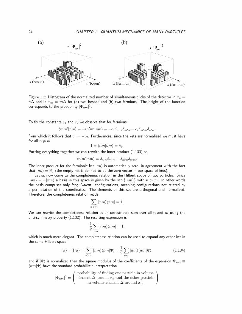
If we now repeat the coincidence experiment N 1 times, count the number of timesthat the detectors click simultaneously in xn and xm and divide the result by N we can drawthe histograms of Fig. 1.2 for bosons and fermions. The probability is symmetric under theinterchange n ↔ m due to property (1.132). The fermions are easily recognizable since theprobability of finding them in the same place is zero.
In these lecture notes we will almost exclusively deal with electrons, which are fermionicparticles. Therefore in the following we will consider the fermionic case only. Let us henceassume that the particles in our one-dimensional world are fermions. The probability of measuringa particle in xn′ and the other in xm′ just after the detectors in xn and xm have simultaneouslyclicked is zero unless n = n′ and m = m′ or n = m′ and m = n′, and hence
〈n′m′|nm〉 = c1δn′nδm′m + c2δm′nδn′m. (1.133)
24 CHAPTER 1. QUANTUM MECHANICS OF MANY PARTICLES
Figure 1.2: Histogram of the normalized number of simultaneous clicks of the detector in xn =n∆ and in xm = m∆ for (a) two bosons and (b) two fermions. The height of the functioncorresponds to the probability |Ψnm|2.
To fix the constants c1 and c2 we observe that for fermions
〈n′m′|nm〉 = −〈n′m′|mn〉 = −c1δn′mδm′n − c2δm′mδn′n,
from which it follows that c1 = −c2. Furthermore, since the kets are normalized we must havefor all n 6= m
1 = 〈nm|nm〉 = c1.
Putting everything together we can rewrite the inner product (1.133) as
〈n′m′|nm〉 = δn′nδm′m − δm′nδn′m.
The inner product for the fermionic ket |nn〉 is automatically zero, in agreement with the factthat |nn〉 = |∅〉 (the empty ket is defined to be the zero vector in our space of kets).
Let us now come to the completeness relation in the Hilbert space of two particles. Since|nm〉 = −|mn〉 a basis in this space is given by the set |nm〉 with n > m. In other wordsthe basis comprises only inequivalent configurations, meaning configurations not related bya permutation of the coordinates. The elements of this set are orthogonal and normalized.Therefore, the completeness relation reads∑
n>m
|nm〉〈nm| = 1,
We can rewrite the completeness relation as an unrestricted sum over all n and m using theanti-symmetry property (1.132). The resulting expression is
1
2
∑nm
|nm〉〈nm| = 1,
which is much more elegant. The completeness relation can be used to expand any other ket inthe same Hilbert space
|Ψ〉 = 1|Ψ〉 =∑n>m
|nm〉〈nm|Ψ〉 =1
2
∑nm
|nm〉〈nm|Ψ〉, (1.134)
and if |Ψ〉 is normalized then the square modulus of the coefficients of the expansion Ψnm ≡〈nm|Ψ〉 have the standard probabilistic interpretation
|Ψnm|2 =
probability of finding one particle in volumeelement ∆ around xn and the other particle
in volume element ∆ around xm

1.2. MANY-PARTICLE QUANTUM MECHANICS 25
for all n 6= m. We can now refine the experiment by putting the detectors closer and closer.The continuum limit works exactly in the same manner as before. We rewrite the expansion(1.134) as
|Ψ〉 =1
2∆2∑nm
|nm〉∆
Ψnm
∆, (1.135)
and define the continuous wavefunction Ψ(xn, xm) and the continuous ket |xnxm〉 according to
Ψ(xn, xm) = lim∆→0
Ψnm
∆, |xnxm〉 = lim
∆→0
|nm〉∆
.
The expansion (1.135) can then be seen as the Riemann sum of Ψ(xn, xm)|xnxm〉 and in thelimit ∆→ 0 the sum becomes the integral
|Ψ〉 =1
2
∫dxdx′ Ψ(x, x′)|xx′〉.
We can also derive the continuous representation of the completeness relation and the continuousrepresentation of the inner product between two basis kets. We have
lim∆→0
1
2∆2∑nm
|nm〉∆
〈nm|∆
=1
2
∫dxdx′|xx′〉〈xx′| = 1. (1.136)
and
lim∆→0
〈n′m′|nm〉∆2
= 〈xn′xm′ |xnxm〉
= δ(xn′ − xn)δ(xm′ − xm)− δ(xm′ − xn)δ(xn′ − xm) (1.137)
The generalization to higher dimensions and to particles with different spin projections is nowstraightforward. We define the position-spin ket |x1x2〉 = |r1σ1 r2σ2〉 as the ket of the physicalstate in which the particles collapse after the simultaneous clicking of a spin-polarized detectorfor particles of spin-projection σ1 placed in r1 and a spin-polarized detector for particles of spin-projection σ2 placed in r2. The set of inequivalent configurations |x1x2〉 forms a basis of theHilbert space of two identical particles. In the following we will refer to this space as H2. Inanalogy with (1.137) the continuous kets have inner product
〈x′1x′2|x1x2〉 = δ(x′1 − x1)δ(x′2 − x2)− δ(x′1 − x2)δ(x′2 − x1)
=∑P
(−1)P δ(x′1 − xP (1))δ(x′2 − xP (2)). (1.138)
The second line of this equation is an equivalent way of rewriting the anti-symmetric product ofδ-functions. The sum runs over the permutations P of (1, 2) which are the identity permutation(P (1), P (2)) = (1, 2) and the interchange (P (1), P (2)) = (2, 1). The quantity (−1)P is equalto +1 if the permutation requires an even number of interchanges and −1 if the permutationrequires an odd number of interchanges.In complete analogy with (1.136) we can also write the completeness relation according to
1
2
∫dx1dx2|x1x2〉〈x1x2| = 1. (1.139)
Then, any ket |Ψ〉 ∈ H2 can be expanded in the position-spin basis as
|Ψ〉 = 1|Ψ〉 =1
2
∫dx1dx2 |x1x2〉 〈x1x2|Ψ〉︸ ︷︷ ︸
Ψ(x1,x2)
. (1.140)

26 CHAPTER 1. QUANTUM MECHANICS OF MANY PARTICLES
If |Ψ〉 is normalized we can give a probability interpretation to the square modulus of the wave-function Ψ(x1,x2)
|Ψ(x1,x2)|2dr1dr2 =
probability of finding one particle with spin σ1 involume element dr1 around r1 and the other particle withspin σ2 in volume element dr2 around another point r2
.
We stress again that the above probability interpretation follows from the normalization 〈Ψ|Ψ〉 =1, which in the continuum case reads [see (1.140)]
1 =1
2
∫dx1dx2 |Ψ(x1,x2)|2.
It should now be clear how to extend the above relations to the case of N identical fermions.We say that if the detector for a particle of spin-projection σ1 placed in r1, the detector for aparticle of spin-projection σ2 placed in r2, etc. all click at the same time then the N -particlestate collapses in the position-spin ket |x1 . . .xN 〉. Due to the nature of identical particles thisket must have the symmetry property
|xP (1) . . .xP (N)〉 = (−1)P |x1 . . .xN 〉 (1.141)
where P is a permutation of the labels (1, . . . , N), and (−1)P = 1 for even permutationsand ±1 for odd permutations. A permutation is even/odd if the number of interchanges iseven/odd. Therefore, given the ket |x1 . . .xN 〉 with all different coordinates there are N !equivalent configurations that represent the same physical state. If two or more coordinates arethe same then the ket |x1 . . .xN 〉 is the null ket |∅〉. The set of position-spin kets correspondingto inequivalent configurations form a basis in the Hilbert space of N identical particles; we willrefer to this space as HN . The inner product between two position-spin kets is
〈x′1 . . .x′N |x1 . . .xN 〉 =∑P
cP
N∏j=1
δ(x′j − xP (j)),
where the cP ’s are numbers depending on the permutation P . Like in the two-particle case theanti-symmetry (1.141) of the position-spin kets requires that cP = c (−1)P , and the normaliza-tion of |x1 . . .xN 〉 with all different coordinates fixes the constant c = 1. Hence
〈x′1 . . .x′N |x1 . . .xN 〉 =∑P
(−1)PN∏j=1
δ(x′j − xP (j)) (1.142)
This is the familiar expression for the determinant |A | of a N ×N matrix A
|A | ≡∑P
(−1)PA1P (1) . . . ANP (N).
Choosing the matrix elements of A to be Aij = δ(x′i − xj) we can rewrite (1.142) as
〈x′1 . . .x′N |x1 . . .xN 〉 =
∣∣∣∣∣∣∣∣δ(x′1 − x1) . . . δ(x′1 − xN )
. . . . .
. . . . .δ(x′N − x1) . . . δ(x′N − xN )
∣∣∣∣∣∣∣∣ . (1.143)

1.2. MANY-PARTICLE QUANTUM MECHANICS 27
Given the norm of the position-spin kets the completeness relation for N particles is a straight-forward generalization of (1.139) and reads
1
N !
∫dx1 . . . dxN |x1 . . .xN 〉〈x1 . . .xN | = 1 (1.144)
Therefore the expansion of a ket |Ψ〉 ∈ HN can be written as
|Ψ〉 = 1|Ψ〉 =1
N !
∫dx1 . . . dxN |x1 . . .xN 〉 〈x1 . . .xN |Ψ〉︸ ︷︷ ︸
Ψ(x1,...,xN )
,
which generalizes the expansion (1.140) to the case ofN particles. The wavefunction Ψ(x1, . . . ,xN )totally antisymmetric for fermions due to (1.141). If |Ψ〉 is normalized then the normalizationof the wavefunction reads
1 = 〈Ψ|Ψ〉 =1
N !
∫dx1 . . . dxN |Ψ(x1, . . . ,xN )|2. (1.145)
The probabilistic interpretation of the square modulus of the wavefunction can be extractedusing the same line of reasoning of the two-particle case
|Ψ(x1 . . .xN )|2N∏j=1
drj =
probability of finding
a particle with spin σ1 in dr1 around around r1 and...
a particle with spin σN in drN around rN
,
(1.146)We could have absorbed the prefactor 1/N ! in (1.145) in the wavefunction (as it is commonlydone) but then we could not interpret the quantity |Ψ(x1, . . . ,xN )|2dr1 . . . drN as the righthand side (r.h.s.) of (1.146) since this would amount to regarding equivalent configurations asdistinguishable and consequently the probability would be overestimated by a factor of N !.
1.2.2 Field operators
The advantage of the bra-and-ket notation invented by Dirac is twofold. First of all, it providesa geometric interpretation of the physical states in Hilbert space as abstract kets independent ofthe basis in which they are expanded. For example, it does not matter whether we expand |Ψ〉in terms of the position-spin kets or momentum-spin kets; |Ψ〉 remains the same although theexpansion coefficients in the two basis are different. The second advantage is that the abstractkets can be systematically generated by repeated applications of a creation operator on theempty or zero-particle state. This approach forms the basis of an elegant formalism known assecond quantization, which we will describe in detail in this Section.
To deal with arbitrary many identical particles we define a collection F of Hilbert spaces,also known as Fock space, according to
F = H0,H1, . . . ,HN , . . .,
with HN the Hilbert space for N identical particles. An arbitrary element of the Fock space isa ket that can be written as
|Ψ〉 =
∞∑N=0
cN |ΨN 〉, (1.147)

28 CHAPTER 1. QUANTUM MECHANICS OF MANY PARTICLES
where |ΨN 〉 belongs to HN . The inner product between the ket (1.147) and another elementin the Fock space
|χ〉 =
∞∑N=0
dN |χN 〉
is defined as
〈χ|Ψ〉 ≡∞∑N=0
d∗NcN 〈χN |ΨN 〉,
where 〈χN |ΨN 〉 is the inner product in HN . This definition is dictated by common sense: theprobability of havingM 6= N particles in a N -particle ket is zero and therefore kets with differentnumber of particles are orthogonal, i.e., have zero overlap.
The Hilbert space H0 is the space with zero particles. Since an empty system has no degreesof freedom H0 is a one-dimensional space and we will denote by |0〉 the only normalized ket inH0,
〈0|0〉 = 1.
According to the expansion (1.147) the ket |0〉 has all cN = 0 except for c0. This state should notbe confused with the null ket |∅〉 which is defined as the state in Fock space with all cN = 0 and,therefore, is not a physical state. The empty ket |0〉 is a physical state; indeed the normalization〈0|0〉 = 1 means that the probability of finding nothing in an empty space is 1.
The goal of this Section is to find a clever way to construct a basis for each Hilbert spaceH1, H2, . . .. To accomplish this goal the central idea of the second quantization formalism is todefine a field operator ψ†(x) = ψ†(rσ) that generates the position-spin kets by repeated actionon the empty ket, i.e.,
|x1〉 = ψ†(x1)|0〉
|x1x2〉 = ψ†(x2)|x1〉 = ψ†(x2)ψ†(x1)|0〉
|x1 . . .xN 〉 = ψ†(xN )|x1 . . .xN−1〉 = ψ†(xN ) . . . ψ†(x1)|0〉
(1.148)
Since an operator is uniquely defined from its action on a complete set of states in the Hilbertspace (the Fock space in our case), the above relations define the field operator ψ†(x) for all x.The field operator ψ†(x) transforms a ket of HN into a ket of HN+1 for all N , see Fig. 1.3(a).We may say that the field operator ψ†(x) creates a particle in x and it is therefore called thecreation operator. Since the position-spin kets change a minus sign under interchange of anytwo particles it follows that
ψ†(x)ψ†(y)|x1 . . .xN 〉 = |x1 . . .xN y x〉 = −|x1 . . .xN x y〉= −ψ†(y)ψ†(x)|x1 . . .xN 〉,
This identity is true for all x1, . . . ,xN and for all N , i.e., for all states in F , and hence
ψ†(x)ψ†(y) = −ψ†(y)ψ†(x).
If we define the anti-commutator between two generic operators A and B according to[A, B
]+
= AB + BA,
we can rewrite the above relation as [ψ†(x), ψ†(y)
]+
= 0 (1.149)
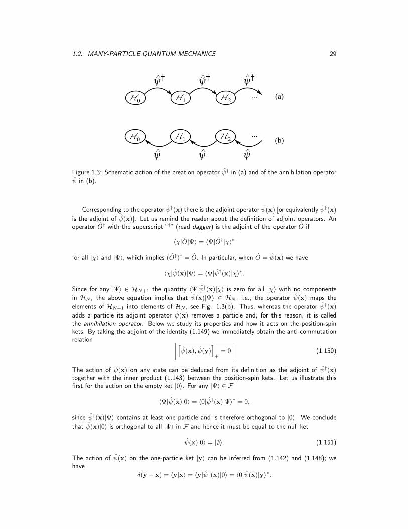
1.2. MANY-PARTICLE QUANTUM MECHANICS 29
Figure 1.3: Schematic action of the creation operator ψ† in (a) and of the annihilation operatorψ in (b).
Corresponding to the operator ψ†(x) there is the adjoint operator ψ(x) [or equivalently ψ†(x)
is the adjoint of ψ(x)]. Let us remind the reader about the definition of adjoint operators. Anoperator O† with the superscript “†” (read dagger) is the adjoint of the operator O if
〈χ|O|Ψ〉 = 〈Ψ|O†|χ〉∗
for all |χ〉 and |Ψ〉, which implies (O†)† = O. In particular, when O = ψ(x) we have
〈χ|ψ(x)|Ψ〉 = 〈Ψ|ψ†(x)|χ〉∗.
Since for any |Ψ〉 ∈ HN+1 the quantity 〈Ψ|ψ†(x)|χ〉 is zero for all |χ〉 with no componentsin HN , the above equation implies that ψ(x)|Ψ〉 ∈ HN , i.e., the operator ψ(x) maps theelements of HN+1 into elements of HN , see Fig. 1.3(b). Thus, whereas the operator ψ†(x)
adds a particle its adjoint operator ψ(x) removes a particle and, for this reason, it is calledthe annihilation operator. Below we study its properties and how it acts on the position-spinkets. By taking the adjoint of the identity (1.149) we immediately obtain the anti-commutationrelation [
ψ(x), ψ(y)]
+= 0 (1.150)
The action of ψ(x) on any state can be deduced from its definition as the adjoint of ψ†(x)together with the inner product (1.143) between the position-spin kets. Let us illustrate thisfirst for the action on the empty ket |0〉. For any |Ψ〉 ∈ F
〈Ψ|ψ(x)|0〉 = 〈0|ψ†(x)|Ψ〉∗ = 0,
since ψ†(x)|Ψ〉 contains at least one particle and is therefore orthogonal to |0〉. We concludethat ψ(x)|0〉 is orthogonal to all |Ψ〉 in F and hence it must be equal to the null ket
ψ(x)|0〉 = |∅〉. (1.151)
The action of ψ(x) on the one-particle ket |y〉 can be inferred from (1.142) and (1.148); wehave
δ(y − x) = 〈y|x〉 = 〈y|ψ†(x)|0〉 = 〈0|ψ(x)|y〉∗.
30 CHAPTER 1. QUANTUM MECHANICS OF MANY PARTICLES
Since ψ(x)|y〉 ∈ H0 it follows that
ψ(x)|y〉 = δ(y − x)|0〉. (1.152)
We see from this relation that the operator ψ(x) removes a particle from the state |y〉 whenx = y and otherwise yields zero. The derivation of the action of ψ(x) on the empty ket and onthe one-particle ket was rather elementary. Let us now derive the action of ψ(x) on the generalN -particle ket |y1 . . .yN 〉. For this purpose we consider the matrix element
〈x1 . . .xN−1|ψ(xN )|y1 . . .yN 〉 = 〈x1 . . .xN |y1 . . .yN 〉. (1.153)
The overlap on the r.h.s. is given in (1.143); expanding the determinant along row N we get
〈x1 . . .xN−1|ψ(xN )|y1 . . .yN 〉
=N∑k=1
(−1)N+kδ(xN − yk)〈x1 . . .xN−1|y1 . . .yk−1yk+1 . . .yN 〉.
This expression is valid for any |x1 . . .xN−1〉 and since ψ(x) maps from HN only to HN−1 weconclude that
ψ(x)|y1 . . .yN 〉 =
N∑k=1
(−1)N+kδ(x− yk) |y1 . . .yk−1yk+1 . . .yN 〉 (1.154)
We just derived an important equation for the action of the annihilation operator on a position-spin ket. It correctly reduces to (1.152) when N = 1 and for N > 1 yields, for example,
ψ(x)|y1y2〉 = δ(x− y2)|y1〉 − δ(x− y1)|y2〉, (1.155)
ψ(x)|y1y2y3〉 = δ(x− y3)|y1y2〉 − δ(x− y2)|y1y3〉+ δ(x− y1)|y2y3〉.
So the annihilation operator removes subsequently a particle from every position-spin coordinatewhile keeping the final result totally symmetric or antisymmetric in all y variables by adjusting thesigns of the prefactors. With the help of (1.154) we can derive a fundamental anti-commutationrelation between the annihilation and creation operators. Acting on both sides of (1.154) withψ†(y) and denoting by |R〉 the ket on the r.h.s. we have
ψ†(y)ψ(x)|y1 . . .yN 〉 = ψ†(y)|R〉. (1.156)
Exchanging the order of the field operators in the left hand side (l.h.s.) of the above identityand using (1.154) we find
ψ(x)ψ†(y)|y1 . . .yN 〉 = ψ(x)|y1 . . .yNy〉 = δ(x− y) |y1 . . .yN 〉
+
N∑k=1
(−1)N+1+kδ(x− yk) |y1 . . .yk−1yk+1 . . .yNy〉
= δ(x− y) |y1 . . .yN 〉 − ψ†(y)|R〉. (1.157)
Addition of (1.156) and (1.157) then gives[ψ(x), ψ†(y)
]+|y1 . . .yN 〉 = δ(x− y)|y1 . . .yN 〉,

1.2. MANY-PARTICLE QUANTUM MECHANICS 31
which must be valid for all position-spin kets and for all N , and therefore[ψ(x), ψ†(y)
]+
= δ(x− y) (1.158)
The anti-commutation relations (1.149), (1.150) and (1.158) are the main results of this Section.As we shall see in Section 1.2.4 all many-particle operators, like total energy, density, current,spin, etc., consist of simple expressions in terms of the field operators ψ and ψ†, and the calcu-lation of their averages can easily be performed with the help of the anti-commutation relations.Using the anti-commutation properties we can manipulate directly the kets and never have todeal with the rather cumbersome expressions of the wavefunctions; the field operators take careof the symmetry of the kets automatically. The great achievement of second quantization iscomparable to that of a programming language. When we program we use a nice and friendlytext-editor to write a code which tells the computer what operations to do, and we do not botherif the instructions given through the text-editor are correctly executed by the machine. A bugin the code is an error in the text of the program (the way we manipulate the field operators)and not an erroneous functioning of some logic gate (the violation of the symmetry propertiesof the many-particle kets).
1.2.3 General basis states
In the previous Section we learned how to construct states of many identical particles with agiven spin and position. The position-spin is, however, just one possible choice of quantumnumbers to characterize every single particle. We will now show how the field operators can beused to construct states of many identical particles in which every particle is labeled by generalquantum numbers, such as momentum, energy, etc.
Let us consider a normalized one-particle ket |n〉. The quantum number n = (sτ) comprisesan orbital quantum number s and the spin projection τ along some quantization axis. Choosingthe quantization axis of the spin to be the same as that of the position-spin ket |x〉 = |rσ〉 theoverlap between |n〉 and |x〉 is
〈x|n〉 ≡ ϕn(x) = ϕs(r)δτσ. (1.159)
The one-particle ket |n〉 can be expanded in the position-spin kets using the completeness relation
|n〉 =
∫dx |x〉〈x|n〉 =
∫dxϕn(x)|x〉 =
∫dxϕn(x)ψ†(x)|0〉. (1.160)
One can easily check that the normalization 〈n|n〉 = 1 is equivalent to say that∫dx|ϕn(x)|2 = 1.
From (1.160) we see that |n〉 is obtained by applying to the empty ket |0〉 the operator
d†n ≡∫dxϕn(x)ψ†(x) (1.161)
i.e., d†n|0〉 = |n〉. We may say that d†n creates a particle with quantum number n. Similarly, ifwe take the adjoint of (1.161)
dn ≡∫dxϕ∗n(x)ψ(x) (1.162)
we obtain an operator that destroys a particle with quantum number n since
dn|n〉 = dnd†n|0〉 =
∫dxdx′ϕ∗n(x)ϕn(x′) ψ(x)ψ†(x′)|0〉︸ ︷︷ ︸
δ(x−x′)|0〉
=
∫dx |ϕn(x)|2|0〉 = |0〉.
32 CHAPTER 1. QUANTUM MECHANICS OF MANY PARTICLES
The operators dn and d†n, being linear combinations of field operators at different x, can acton states with arbitrary many particles. Below we derive some important relations for the d-operators when the set |n〉 forms an orthonormal basis in the one-particle Hilbert space.
We can easily derive the important anti-commutation relations using the corresponding re-lations for the field operators[
dn, d†m
]+
=
∫dxdx′ ϕ∗n(x)ϕm(x′)
[ψ(x), ψ†(x′)
]+︸ ︷︷ ︸
δ(x−x′)
= 〈n|m〉 = δnm, (1.163)
and the more obvious ones [dn, dm
]+
=[d†n, d
†m
]+
= 0, (1.164)
that follow similarly. It is worth noticing that the d-operators obey the same anti-commutationrelations as the field operators with the index n playing the role of x. This is a very importantobservation since the results of the previous Section relied only on the anti-commutation relationsof ψ and ψ†, and hence remain valid in this more general basis. To convince the reader of thisfact we derive some of the results of the previous Section directly from the anti-commutationrelations. We define the N -particle ket
|n1 . . . nN 〉 ≡ d†nN . . . d†n1|0〉 = d†nN |n1 . . . nN−1〉 (1.165)
which has the symmetry property
|nP (1) . . . nP (N)〉 = (−1)P |n1 . . . nN 〉,
as follows immediately from (1.164). Like the position-spin kets the kets |n1 . . . nN 〉 span theN -particle Hilbert space HN . The action of dn on |n1 . . . nN 〉 is similar to the action of ψ(x) on|x1 . . .xN 〉. Using the anti-commutation relation (1.163) we can move the dn-operator throughthe string of d†-operators3
dn|n1 . . . nN 〉 =
([dn, d
†nN
]+− d†nN dn
)|n1 . . . nN−1〉
= δnnN |n1 . . . nN−1〉 − d†nN
([dn, d
†nN−1
]+− d†nN−1
dn
)|n1 . . . nN−2〉
= δnnN |n1 . . . nN−1〉 − δnnN−1|n1 . . . nN−2nN 〉
(−1)2d†nN d†nN−1
([dn, d
†nN−2
]+− d†nN−2
dn
)|n1 . . . nN−3〉
=
N∑k=1
(−1)N+kδnnk |n1 . . . nk−1nk+1 . . . nN 〉. (1.166)
This result can also be used to calculate directly the overlap between two states of the generalbasis. For example, for the case of two particles we have
〈n′1n′2|n1n2〉 = 〈n′1|dn′2 |n1n2〉 = 〈n′1|(δn′2n2
|n1〉 − δn′2n1|n2〉
)= δn′1n1
δn′2n2− δn′1n2
δn′2n1,
which is the analog of (1.138). More generally, for N particles we have
〈n′1 . . . n′N |n1 . . . nN 〉 =∑P
(−1)PN∏j=1
δn′j nP (j), (1.167)
3Alternatively (1.166) can be derived from (1.154) together with the definitions of the d-operators.

1.2. MANY-PARTICLE QUANTUM MECHANICS 33
which should be compared with the overlap 〈x′1 . . .x′N |x1 . . .xN 〉 in (1.142).The states |n1 . . . nN 〉 are orthonormal and can be used to construct a basis. In analogy
with (1.144) the completeness relation is
1
N !
∑n1,...,nN
|n1 . . . nN 〉〈n1 . . . nN | = 1
and hence the expansion of a ket |Ψ〉 belonging to HN reads
|Ψ〉 = 1|Ψ〉 =1
N !
∑n1,...,nN
|n1 . . . nN 〉 〈n1 . . . nN |Ψ〉︸ ︷︷ ︸Ψ(n1,...,nN )
. (1.168)
If |Ψ〉 is normalized then the coefficients Ψ(n1, . . . , nN ) have the following probabilistic inter-pretation
|Ψ(n1 . . . nN )|2 =
probability of finding
a particle with quantum number n1 and...
a particle with quantum number nN
.
We already observed that the d-operators obey the same (anti)commutation relations as thefield operators provided that |n〉 is an orthonormal basis in H1. Likewise we can constructlinear combinations of the d-operators that preserve the (anti)commutation relations. It is leftas an exercise for the reader to prove that the operators
cα =∑n
Uαndn, c†α =∑n
U∗αnd†n
obey [cα, c
†β
]∓
= δαβ
provided thatUαn ≡ 〈α|n〉
is the inner product between the elements of the original orthonormal basis |n〉 and theelements of another orthonormal basis |α〉. Indeed in this case the Uαn are the matrix elementsof a unitary matrix since∑
n
UαnU†nβ =
∑n
〈α|n〉〈n|β〉 = 〈α|β〉 = δαβ ,
where we used the completeness relation. In particular, when α = x we have Uxn = 〈x|n〉 =
ϕn(x) and we find that cx = ψ(x). We thus recover the field operators as
ψ(x) =∑n
ϕn(x)dn, ψ†(x) =∑n
ϕ∗n(x)d†n. (1.169)
The above relations tell us that the expansion of the position-spin kets in terms of the kets|n1 . . . nN 〉 is simply
|x1 . . .xN 〉 =∑
n1...nN
ϕ∗n1(x1) . . . ϕ∗nN (xN )|n1 . . . nN 〉 (1.170)

34 CHAPTER 1. QUANTUM MECHANICS OF MANY PARTICLES
Conversely, using (1.161) we can expand the general basis kets in terms of the position-spinskets as
|n1 . . . nN 〉 =
∫dx1 . . . dxN ϕn1
(x1) . . . ϕnN (xN )|x1 . . .xN 〉 (1.171)
If we are given a state |Ψ〉 that is expanded in a general basis and we subsequently want tocalculate properties in position-spin space, such as the particle density or the current density,we need to calculate the overlap between |n1 . . . nN 〉 and |x1 . . .xN 〉. This overlap is thewavefunction for N particles with quantum numbers n1, . . . , nN
Ψn1...nN (x1, . . . ,xN ) = 〈x1 . . .xN |n1 . . . nN 〉.
The explicit form of the wavefunction follows directly from the inner product (1.143) and fromthe expansion (1.171), and reads
Ψn1...nN (x1, . . . ,xN ) =∑P
(−1)Pϕn1(xP (1)) . . . ϕnN (xP (N))
=
∣∣∣∣∣∣∣∣ϕn1
(x1) . . . ϕn1(xN )
. . . . .
. . . . .ϕnN (x1) . . . ϕnN (xN )
∣∣∣∣∣∣∣∣ . (1.172)
Since for any matrix A we have |A | = |AT | with AT the transpose of A we can equivalentlywrite
Ψn1...nN (x1, . . . ,xN ) =
∣∣∣∣∣∣∣∣ϕn1
(x1) . . . ϕnN (x1). . . . .. . . . .
ϕn1(xN ) . . . ϕnN (xN )
∣∣∣∣∣∣∣∣ .The determinant is also known as the Slater determinant. For those readers already familiarwith Slater determinants we note that the absence on the r.h.s. of the prefactor 1/
√N ! is a
consequence of forcing on the square modulus of the wavefunction a probability interpretation,as discussed before.
1.2.4 The many-particle Hamiltonian
Let us now discuss the many-particle Hamiltonian. The Hamiltonian operator for N identicalparticles has the same structure as in classical mechanics and has the form
H = T + V + W (1.173)
where
T =
N∑j=1
p2j
2m(1.174)
V =
N∑j=1
v(xj) (1.175)
W =
N∑i>j
w(xi,xj) (1.176)
The operators T , V and W represent the kinetic energy, the potential energy due to the externalfield v(x) and the two-particle interaction. We leave open the possibility that the external field

1.2. MANY-PARTICLE QUANTUM MECHANICS 35
can act on the spins (as in a magnetic field). The two-particle interaction w(x1,x2) = w(x2,x1)is, in general, not spin dependent and of the form w(x1,x2) = v(r1, r2). It is, however,convenient to keep its form general for the moment. The operators V and W are diagonal inposition-spin basis, i.e.
V |x1, . . . ,xN 〉 =
N∑j=1
v(xj)|x1, . . . ,xN 〉 (1.177)
W |x1, . . . ,xN 〉 =
N∑i>j
w(xi,xj)|x1, . . . ,xN 〉 (1.178)
This fact makes it easy to write these operators in second quantization. Let us start by definingan operator that will play an important role in these Lectures:
n(x) = ψ†(x)ψ(x) . (1.179)
This is the so called density operator. To see what the operator does we act with is on atwo-particle ket:
n(x)|x1x2〉 = ψ†(x)ψ(x)|x1x2〉 = ψ†(x) (δ(x− x2)|x1〉 − δ(x− x1)|x2〉)= δ(x− x2)|x1x〉 − δ(x− x1)|x2x〉= (δ(x− x1) + δ(x− x2)) |x1x2〉 (1.180)
You can check for yourself that, in general, we have
n(x)|x1, . . . ,xN 〉 =
N∑j=1
δ(x− xj)|x1, . . . ,xN 〉 (1.181)
We see that if we multiply both sides with v(x) and integrate over x, we obtain exactlyEq.(1.177). We can therefore write the operator V as
V =
∫dx v(x) n(x) =
∫dx v(x) ψ†(x)ψ(x) (1.182)
From Eq.(1.181) we further see that
W |x1, . . . ,xN 〉 =
1
2
N∑i,j=1
w(xi,xj)−1
2
N∑j=1
w(xj ,xj)
|x1, . . . ,xN 〉
=
(1
2
∫dx dx′ w(x,x′)n(x)n(x′)− 1
2
∫dxw(x,x)n(x)
)|x1, . . . ,xN 〉
Using the anti-commutation relations, we can then write
W =1
2
∫dx dx′ w(x,x′)n(x)n(x′)− 1
2
∫dxw(x,x)n(x)
=1
2
∫dx dx′ w(x,x′)
(ψ†(x)ψ(x)ψ†(x′)ψ(x′)− δ(x− x′)ψ†(x)ψ(x)
)=
1
2
∫dx dx′ w(x,x′) ψ†(x)ψ†(x′)ψ(x′)ψ(x). (1.183)

36 CHAPTER 1. QUANTUM MECHANICS OF MANY PARTICLES
We therefore easily find V and W in second quantized form. It remains to express T in secondquantization. This operator is not diagonal in position space, but it is almost. The generalizationof Eq.(1.62) gives
〈x1, . . . ,xN |T |Ψ〉 =1
2m
N∑j=1
〈x1, . . . ,xN |p2j |Ψ〉
= − ~2
2m
N∑j=1
∇2j 〈x1, . . . ,xN |Ψ〉 (1.184)
We will now show that the same matrix elements can be obtained from the following secondquantized form of the kinetic energy
T = − ~2
2m
∫dx ψ†(x)∇2ψ(x) (1.185)
Here the action of the differential operator ∇2 on a field operator is defined via its action onmatrix elements, i.e.
〈Φ|ψ†(x)∇2ψ(x)|Ψ〉 ≡ limr′→r∇′ 2〈Φ|ψ†(rσ)ψ(r′σ)|Ψ〉
Let us check that Eq.(1.185) has the required matrix elements of Eq. (1.184). We start with asmall example and calculate (using the adjoints of Eq.(1.155))
〈x1x2|ψ†(x)ψ(x′) = (δ(x− x2)〈x1| − δ(x− x1)〈x2|) ψ(x′)
= δ(x− x2)〈x1x′| − δ(x− x1)〈x2x
′|= δ(x− x1)〈x′x2|+ δ(x− x2)〈x′x2|
It is not difficult to check yourself that, in general, we have
〈x1, . . . ,xN |ψ†(x)ψ(x′) =
N∑j=1
δ(x− xj)〈x1, . . . ,xj−1,x′,xj+1, . . . ,xN | (1.186)
From this equation it follows that
〈x1, . . . ,xN |ψ†(x)∇2ψ(x)|Ψ〉 = limr′→r∇′ 2〈x1, . . . ,xN |ψ†(x)ψ(r′σ)|Ψ〉
= limr′→r
N∑j=1
δ(x− xj)∇′ 2〈x1, . . . ,xj−1, r′σ,xj+1, . . . ,xN ||Ψ〉
=
N∑j=1
δ(x− xj)∇2〈x1, . . . ,xj−1,x,xj+1, . . . ,xN |
Multiplying both sides with −~2/(2m) and integrating over x gives
− ~2
2m
∫dx 〈x1, . . . ,xN |ψ†(x)∇2ψ(x)|Ψ〉 = − ~2
2m
N∑j=1
∇2j 〈x1, . . . ,xN |Ψ〉
which is exactly what we wanted to prove. Summarizing, we find that the Hamiltonian of amany-particle system can be written as
H =
∫dx ψ†(x)
(− ~2
2m∇2 + v(x)
)ψ(x)
+1
2
∫dx dx′ w(x,x′) ψ†(x)ψ†(x′)ψ(x′)ψ(x). (1.187)

1.2. MANY-PARTICLE QUANTUM MECHANICS 37
If we now introduce a one-particle Hamiltonian h defined by the matrix elements
〈x|h|x′〉 ≡ − ~2
2m∇2δ(x− x′) + v(x)δ(x− x′) (1.188)
Then we can write the one-body part, H0 = T + V , of the Hamiltonian as
H0 =
∫dxdx′ ψ†(x)〈x|h|x′〉ψ(x′) (1.189)
Let us now consider a system of noninteracting particles, i.e. W = 0 and H = H0. We will tryto find the eigenstates of this system. We start out by defining the one-particle states |n〉 by
h|n〉 = εn|n〉. (1.190)
The states |n〉 are the eigenstates of h. We can give a more explicit equation in position basis.If we define ϕn(x) = 〈x|n〉 then we see that by acting with 〈x| on the equation above that
εn〈x|n〉 = 〈x|h|n〉 =
∫dx′〈x|h|x′〉〈x′|n〉 (1.191)
from which it follows that (− ~2
2m∇2 + v(x)
)ϕn(x) = εnϕn(x) (1.192)
We now go back to expression (1.189) Inserting a completeness relation between h and |x′〉 wefind
H0 =∑n
∫dxdx′ ψ†(x)〈x|h|n〉〈n|x′〉ψ(x′)
=∑n
εn
∫dx ψ†(x) 〈x|n〉︸ ︷︷ ︸
ϕn(x)
∫dx′ 〈n|x′〉︸ ︷︷ ︸
ϕ∗n(x′)
ψ(x′) =∑n
εnd†ndn, (1.193)
where we used h|n〉 = εn|n〉 as well as the definitions (1.161) and (1.162) in terms of theone-particle states ϕn. The d-operators bring the Hamiltonian into a diagonal form, i.e., noneof the off-diagonal combinations d†ndm with m 6= n appear in H0. The occupation operator
nn ≡ d†ndn (1.194)
is the analog of the density operator n(x) in the position-spin basis; it counts how many particleshave quantum number n. Using the anti-commutation relations (1.163) and (1.164) it is easyto prove that [
nn, d†m
]−
= δnmd†m,
[nn, dm
]−
= −δnmdm. (1.195)
The action of H0 on |n1 . . . nN 〉 = d†N . . . d†1|0〉 is then
H0 d†nN d
†nN−1
. . . d†n1|0〉︸ ︷︷ ︸
|n1...nN 〉
=∑n
εn
([nn, d
†nN
]−d†nN−1
. . . d†n1|0〉
+ d†nN
[nn, d
†nN−1
]−. . . d†n1
|0〉
...
+ d†nN d†nN−1
. . .[nn, d
†n1
]−|0〉)
= (εn1+ . . .+ εnN ) d†nN d
†nN−1
. . . d†n1|0〉. (1.196)

38 CHAPTER 1. QUANTUM MECHANICS OF MANY PARTICLES
We thus find thatH0|n1, . . . , nN 〉 = (εn1
+ . . .+ εnN )|n1, . . . , nN 〉 (1.197)
and we therefore have found that the states |n1, . . . , nN 〉 are the eigenstates of H0. Since thesestates form a complete set there are no other eigenstates and we have completely solved theeigenvalue problem. The states in position-spin basis are given by the Slater determinant ofEq.(1.172).

Chapter 2
Density and density matrices
2.1 Correlation functions
2.1.1 The particle density
We will now come to the discussion of the main player of these Lecture Notes, namely theparticle density. The concept can be easily defined for arbitrary types of particles, but we willmostly focus on the case case of electronic systems. In that case the particle density is identicalto the electron density. The concept of density is closely related to that of probablity density.To illustrate this let us, for simplicity, consider a system of spinless fermions in one dimension.Then the position kets |x1 . . . xN 〉 with x1 > . . . > xN form a basis in the N -particle Hilbertspace HN . Any state |Ψ〉 ∈ HN can be expanded as
|Ψ〉 =
∫x1>...>xN
dx1 . . . dxN |x1 . . . xN 〉 〈x1 . . . xN |Ψ〉︸ ︷︷ ︸Ψ(x1,...,xN )
and the normalization condition reads
1 = 〈Ψ|Ψ〉 =
∫x1>...>xN
dx1 . . . dxN 〈Ψ|x1 . . . xN 〉〈x1 . . . xN |Ψ〉
=1
N !
∫dx1 . . . dxN |Ψ(x1, . . . , xN )|2. (2.1)
Let us now ask what is the probability density p(z) for finding a particle at position z. We startwith the first nontrivial case of N = 2 particles. The basis states are then formed by the states|xy〉 for x > y. This configuration space is given by the grey area in the figure below
y
xz
(x,z)
(z,y)
x>y
39

40 CHAPTER 2. DENSITY AND DENSITY MATRICES
We then have
p(z) =
∫ ∞z
dx |Ψ(x, z)|2 +
∫ z
−∞dy |Ψ(z, y)|2 =
∫ ∞−∞
dy|Ψ(z, y)|2 (2.2)
where in the last equality we used the antisymmetry of the wavefunction. We observe, however,that ∫ ∞
−∞dz p(z) =
∫ ∞−∞
dzdy |Ψ(z, y)|2 = 2
as follows directly from (2.1). Intuitively, it seems strange that a probability does not integrateto unity and therefore an explanation is needed. The resolution of this apparent paradox is thatwe do not deal with independent events. Let us, for example fix two points z and z′ with z > z′.The probability to find a particle in z is p(z) whereas the probability to find a particle in z′
is p(z′). What is the probability to find a particle in z or z′? If these probabilities p(z) wereindependent this would simply be p(z) + p(z′). This is, however, not the case because the state|z, z′〉, describing a particle at z and another at z′ contributes to the integral (2.2) for bothp(z) and p(z′) and is counted twice. The fact that we find a particle in z does not excludethe possibility to find another at z′ and we therefore do not deal with probabilities of exclusiveevents. The proper probability formula for overlapping event sets A and B is
p(A ∪B) = p(A) + p(B)− p(A ∩B).
One may object that only the single point y = z′ matters in the integral (2.2) which is of measurezero. However, these points do give a finite contribution when we subsequently integrate over z.To avoid this issue let us therefore illustrate the problem once more by a simple discrete example.Consider two bosons that can either occupy state |1〉 or state |2〉. Then the two-particle Hilbertspace is given by H2 = |11〉, |12〉, |22〉. Since we deal with bosons we have |12〉 = |21〉. Ageneral state describing these two particles is a linear combination of the basis states in H2
|Ψ〉 = Ψ(1, 1)|11〉+ Ψ(1, 2)|12〉+ Ψ(2, 2)|22〉,
and if |Ψ〉 is normalized we have
|Ψ(1, 1)|2 + |Ψ(1, 2)|2 + |Ψ(2, 2)|2 = 1.
Now the probability to find a particle in state 1 is
p(1) = |Ψ(1, 1)|2 + |Ψ(1, 2)|2.
Similarly the probability to find a particle in state 2 is
p(2) = |Ψ(1, 2)|2 + |Ψ(2, 2)|2.
However, the probability to find a particle in state 1 or in state 2 is not the sum of the twoprobabilities since
p(1) + p(2) = |Ψ(1, 1)|2 + 2|Ψ(1, 2)|2 + |Ψ(2, 2)|2 = 1 + |Ψ(1, 2)|2.
In this way we double count the state |12〉. The fact that we do find a particle in state 1 does notexclude the fact that another particle can be found in state 2. This joint probability is |Ψ(1, 2)|2and needs to be subtracted from p(1) + p(2). In this way the probability to find a particle eitherin |1〉 or |2〉 is unity, as it should.We now go back to the continuum problem of two spinless fermions on a line. Let us now ask
2.1. CORRELATION FUNCTIONS 41
for the probability that we find a particle in the interval [z1, z2]. It will be convenient to firstdefine the following integration regions
A = (x, y) |x > y and x ∈ [z1, z2]B = (x, y) |x > y and y ∈ [z1, z2]
A ∩B = (x, y) |x > y and x ∈ [z1, z2] and y ∈ [z1, z2]
To find the probability π(z1, z2) that a particle is in the interval [z1, z2] we have to integrateover A and B but subtract the overlapping region A ∩ B otherwise we would count the regionA ∩B twice. We therefore have
π(z1, z2) =
∫A
dxdy |Ψ(x, y)|2 +
∫B
dxdy |Ψ(x, y)|2 −∫A∩B
dxdy |Ψ(x, y)|2
=
∫ z2
z1
dx
∫ ∞−∞
dy θ(x− y)|Ψ(x, y)|2 +
∫ z2
z1
dy
∫ ∞−∞
dx θ(x− y)|Ψ(x, y)|2
−∫ z2
z1
dx
∫ z2
z1
dy θ(x− y)|Ψ(x, y)|2
=
∫ z2
z1
dx
∫ ∞−∞
dy |Ψ(x, y)|2 − 1
2
∫ z2
z1
dx
∫ z2
z1
dy |Ψ(x, y)|2
=
∫ z2
z1
dx p(x)− 1
2
∫ z2
z1
dx
∫ z2
z1
dy |Ψ(x, y)|2 (2.3)
where we used that fact that |Ψ(x, y)| = |Ψ(y, x)|. In the limit z1 → −∞ and z2 →∞ the firstterm in the last line becomes equal to 2 and the last term equal to −1 such that the probabilityto find a particle anywhere is equal to one as it should, i.e. π(−∞,∞) = 1. Let us now considera small interval [z −∆/2, z + ∆/2] then we find that
π(z − ∆
2, z +
∆
2) =
∫ z+ ∆2
z−∆2
dx p(x)− 1
2
∫ z+ ∆2
z−∆2
dx
∫ z+ ∆2
z−∆2
dy |Ψ(x, y)|2
= p(z)∆ +O(∆2) (∆→ 0) (2.4)
or equivalently
lim∆→0
π(z − ∆2 , z + ∆
2 )
∆= p(z). (2.5)
We therefore see that, although p(z) does not integrate to one, the quantity p(z)∆ still givesthe probability to find a particle in a small interval ∆ around the point z. This becomes exactin the limit ∆→ 0.So far we discussed the case of two spinless particles. Let us now calculate the probability densityp(z) for N spinless fermions in one dimension. We have
p(z) =
∫z>x2>...>xN
dx2 . . . dxN |Ψ(z, x2, . . . , xN )|2
+
∫x1>z>x3>...>xN
dx1dx3 . . . dxN |Ψ(x1, z, x3, . . . , xN )|2
+ . . .+
∫x1>...>xN−1>z
dx1 . . . dxN−1|Ψ(x1, . . . , xN−1, z)|2
=
∫x2>...>xN
dx2 . . . dxN |Ψ(z, x2, . . . , xN )|2
=1
(N − 1)!
∫dx2 . . . dxN |Ψ(z, x2, . . . , xN )|2, (2.6)

42 CHAPTER 2. DENSITY AND DENSITY MATRICES
where we used the antisymmetry of the wavefunction. As in the previous case p(z) is the densityof particles in z and does not integrate to unity but to the total number of particles N , i.e.
N =
∫ ∞−∞
dz p(z) (2.7)
as follows immediately from Eq.(2.1). The reason is the same as before. Let us now show thatthe probability p(z) is simply given as the expectation value of a familiar operator, namely thedensity operator n(z). We have
p(z) = 〈Ψ|n(z)|Ψ〉 = 〈Ψ|ψ†(z)ψ(z)|Ψ〉 (2.8)
This follows from a short calculation. We have
〈Ψ|ψ†(z)ψ(z)|Ψ〉 =
∫x2>...>xN
dx2 . . . dxN 〈Ψ|ψ†(z)|x2 . . . xN 〉〈x2 . . . xN |ψ(z)|Ψ〉
=1
(N − 1)!
∫dx2 . . . dxN 〈Ψ|x2 . . . xNz〉〈x2 . . . xNz|Ψ〉
=1
(N − 1)!
∫dx2 . . . dxN |Ψ(z, x2, . . . , xN )|2 (2.9)
which is equal to the expression (2.6). In the following we will therefore use the notationn(z) = p(z). Clearly the above derivation can readily be generalized to particles with spin,dimensions higher than 1, and to the bosonic case. We define the particle density by
n(x) = 〈Ψ|n(x)|Ψ〉 = 〈Ψ|ψ†(x)ψ(x)|Ψ〉 (2.10)
Thus the physical interpretation of the density n(x) = n(r, σ) is that n(r, σ)∆V is the probabilityof finding a particle with spin-projection σ in volume ∆V around point r. This becomes exactin the limit ∆V → 0. The density integrates to N particles,
N =
∫dxn(x) =
∑σ=±1
∫drn(r, σ) (2.11)
as a consequence of the fact that we do not deal with exclusive probabilities.
2.1.2 The pair density and other correlation functions
Coming back to our one-dimensional system of fermions we now consider the joint probabilityp(z, z′) of finding a particle at z and another at z′. We again consider a state |Ψ〉 describing Nparticles. Since p(z, z′) = p(z′, z) we can assume that z > z′. Then
p(z, z′) =
∫z>z′>x3>...>xN
dx3 . . . dxN |Ψ(z, z′, x3, . . . , xN )|2
+
∫z>x2>z′>...>xN
dx2dx4 . . . dxN |Ψ(z, x2, z′, . . . , xN )|2
+ . . . +
∫x1>z>z′>...>xN
dx1dx4 . . . dxN |Ψ(x1, z, z′, . . . , xN )|2 + . . .
=
∫x3>...>xN
dx3 . . . dxN |Ψ(z, z′, x3, . . . , xN )|2 =
=1
(N − 2)!
∫dx3 . . . dxN |Ψ(z, z′, x3, . . . , xN )|2, (2.12)

2.1. CORRELATION FUNCTIONS 43
where again the antisymmetry of the wavefunction has been used. The probability p(z, z′) isreferred to as the pair density. We can rewrite the pair density in terms of the field operators as
p(z, z′) = 〈Ψ|ψ†(z)ψ†(z′)ψ(z′)ψ(z)|Ψ〉. (2.13)
This is readily verified. Analogously to Eq.(2.9) we have
〈Ψ|ψ†(z)ψ†(z′)ψ(z′)ψ(z)|Ψ〉
=
∫x3>...>xN
dx3 . . . dxN 〈Ψ|ψ†(z)ψ†(z′)|x3 . . . xN 〉〈x3 . . . xN |ψ(z′)ψ(z)|Ψ〉
=1
(N − 2)!
∫dx3 . . . dxN 〈Ψ|x3 . . . xNz
′z〉〈x2 . . . xNz′z|Ψ〉
=1
(N − 2)!
∫dx3 . . . dxN |Ψ(z, z′, x3, . . . , xN )|2 (2.14)
which is identical to the expression calculated in Eq.(2.12). It is readily checked that the pair-density satisfies
(N − 1) p(z) =
∫dz′ p(z, z′). (2.15)
Again it is clear that the derivations can be repeated for particles with spin in three dimensions.We therefore define the pair-density operator as
Γ(x,x′) = ψ†(x)ψ†(x′)ψ(x′)ψ(x) (2.16)
and the pair-density itself for a state |Ψ〉 as the expectation value
Γ(x,x′) = 〈Ψ|Γ(x,x′)|Ψ〉 (2.17)
The physical interpretation of this quantity is that the probability to find a particle with spin σin volume ∆V around r and another particle with spin σ′ in volume ∆V ′ around r′ is given byΓ(x,x′)∆V∆V ′. Again, this becomes exact in the limit ∆V,∆V ′ → 0. If the particles wherecompletely independent then the probability the find a particle at x and x′ would simply be theproduct n(x)n(x′). Therefore, one often define a pair-correlation function denoted by g(x,x′)to measure the deviation from this product. Its explicit definition is
g(x,x′) =Γ(x,x′)
n(x)n(x′). (2.18)
We will study this function in more detail later. Another very useful concept is the conditionaldensity ρ(x|x′) which gives the conditional probability to find a particle at x, given that we knowthat there is a particle at x′. This function is defined as
ρ(x|x′) =Γ(x,x′)
n(x′). (2.19)
Whenever the particles are completely uncorrelated then Γ(x,x′) = n(x)n(x′) and ρ(x|x′) =n(x). Then the conditional density to find a particle at x is completely independent on whetherwe found already a particle at x′. The difference ρ(x|x′)−n(x) therefore measures the amountof correlations in the system, and is called the exchange-correlation hole. It explicit form is
ρxc(x|x′) =Γ(x,x′)
n(x′)− n(x) = n(x)(g(x,x′)− 1). (2.20)

44 CHAPTER 2. DENSITY AND DENSITY MATRICES
It is therefore the difference between the conditional and unconditional density of finding aparticle at x. The origin of the name exchange-correlation (xc) will be explained in more detailin later sections. In a correlated system of electrons the probability to find an electron close toa reference electron at position x′ is reduced as compared to the uncorrelated case described bythe density profile n(x). The function ρxc therefore effectively digs a hole in the unconditionaldensity distribution. The volume of this hole is given by∫
dx ρxc(x|x′) =1
n(x′)
∫dx Γ(x,x′)−
∫dxn(x)
=1
n(x′)(N − 1)n(x′)−N = −1. (2.21)
The hole therefore integrates to minus one electron. For later reference we also write this interms of the pair-correlation function
−1 =
∫dxn(x)(g(x,x′)− 1). (2.22)
So far we defined these functions with inclusion of spin-coordinates. We can also ask for theprobability to find a particle with any spin polarization at position r. Then we simply have tosum the density n(x) = n(r, σ) over its spin coordinate. The same applies to the pair-density.We can therefore define the operators
n(r) =∑σ=±1
n(r, σ) (2.23)
Γ(r, r′) =∑
σ,σ′=±1
Γ(rσ, r′σ′) (2.24)
with expectation values
n(r) = 〈Ψ|n(r)|Ψ〉 (2.25)Γ(r, r′) = 〈Ψ|Γ(r, r′)|Ψ〉. (2.26)
The density n(r) probability to find a particle with any spin at r, whereas the pair-density Γ(r, r′)gives the probability to find a particle at r and another at r′ independent of their spin projections.The pair-correlation function and the xc-hole for the spin-integrated case are be defined in thesame way as before
g(r, r′) =Γ(r, r′)
n(r)n(r′)(2.27)
ρxc(r|r′) =Γ(r, r′)
n(r′)− n(r) (2.28)
You can check for yourself that again we have the sumrule
−1 =
∫dr ρxc(r|r′) =
∫drn(r)(g(r, r′)− 1). (2.29)
We come back to these functions after we have studied density matrices.
2.2 Density matrices
2.2.1 General properties
In this section we will generalize the density and pair-density to higher order correlation functions,namely to n-particle density matrices. The reason for this is two-fold. First of all we will show

2.2. DENSITY MATRICES 45
that we can write any n-body operator in terms of the n-particle density matrix. Secondly, wewill derive a simple form for the n-particle density matrix for noninteracting particles that willbe useful later. Let us simply start with the definition. The n-particle density matrix operator isdefined as
Γn(y1, . . . ,yn,x1, . . . ,xn) = ψ†(x1) . . . ψ†(xn)ψ†(yn) . . . ψ†(y1). (2.30)
These operators clearly represent a generalization of the density and pair-density operators thatwe introduced earlier. In particular, we have
n(x) = Γ1(x,x) (2.31)Γ(x,x′) = Γ2(x,x′,x,x′). (2.32)
We denote the expectation value of Γn over a state |Ψ〉 by Γn, i.e.
Γn(y1, . . . ,yn,x1, . . . ,xn) = 〈Ψ|Γn(y1, . . . ,yn,x1, . . . ,xn)|Ψ〉. (2.33)
If the state |Ψ〉 ∈ HN is a Fock-space state for N fermionic particles then Γn is non-vanishingfor n = 0, . . . , N . Let us start by looking at the case n = N . Then
ΓN (y1, . . . ,yN ,x1, . . . ,xN )
= 〈Ψ|ψ†(x1) . . . ψ†(xN )|0〉〈0|ψ†(yN ) . . . ψ†(y1)|Ψ〉 (2.34)= 〈Ψ|xN . . .x1〉〈yN . . .y1|Ψ〉= Ψ(y1, . . . ,yN )Ψ∗(x1, . . . ,xN ). (2.35)
Therefore the N -particle density matrix is just the product of the N -particle wave functions.Let us now consider the general case of the n-particle density matrix. Similarly, by inserting acomplete set of (N − n)-body states |zn+1, . . . , zN 〉 we can readily derive that
Γn(y1, . . . ,yn,x1, . . . ,xn) =
1
(N − n)!
∫dzn+1 . . . dzN Ψ(y1 . . .yn, zn+1 . . . zN )Ψ∗(x1 . . .xn, zn+1 . . . zN ).
From this we see also immediately that
(N − n+ 1)Γn−1(y1 . . .yn−1,x1 . . .xn−1) =
∫dz Γn(y1 . . .yn−1, z,x1 . . .xn−1, z). (2.36)
So far the general properties. Let us now derive the form of these density matrices for a non-interacting state of the form
|Ψ〉 = |n1 . . . nN 〉 = d†nN . . . d†n1|0〉. (2.37)
We start by calculating the one-particle density matrix. If we denote ϕn(x) = 〈x|n〉 we have
Γ1(y,x) = 〈Ψ|ψ†(x)ψ(y)|Ψ〉=
∑kl
ϕ∗k(x)ϕl(y)〈n1 . . . nN |d†kdl|n1 . . . nN 〉
=∑kl
ϕ∗k(x)ϕl(y)〈n1 . . . nN |d†kN∑j=1
(−1)N+jδlnj |n1 . . . nj−1, nj+1 . . . nN 〉
=∑k
N∑j=1
ϕ∗k(x)ϕnj (y) 〈n1 . . . nN |n1 . . . nj−1, k, nj+1 . . . nN 〉
=∑k
N∑j=1
ϕ∗k(x)ϕnj (y)δnjk =
N∑j=1
ϕnj (y)ϕ∗nj (x). (2.38)

46 CHAPTER 2. DENSITY AND DENSITY MATRICES
Therefore the one-particle density matrix is simply the sum of the products of the one-particlestates. In particular, we see that the one-particle density is given by
n(x) = Γ1(x,x) =
N∑j=1
|ϕnj (x)|2. (2.39)
The density is therefore simply the sum of the one-particle densities. For the special form ofEq.(2.38) the one-particle density matrix has the special property that
∫dy Γ1(x,y)Γ1(y, z) =
N∑j,k=1
∫dyϕnj (x)ϕ∗nj (y)ϕnk(y)ϕ∗nk(z)
=
N∑j
ϕnj (x)ϕ∗nj (z) = Γ1(x, z) (2.40)
where we used the orthonormality 〈nj |nk〉 = δjk of the one-particle states. The property (2.40)of the density matrix for the state (2.37) is called idempotency. We will use this property later.Now we take the other extreme and calculate the N -particle density matrix. From Eq.(2.35) wesee that
ΓN (y1 . . .yN ,x1 . . .xN ) = Ψ(y1 . . .yN )Ψ∗(x1 . . .xN )
=
∣∣∣∣∣∣∣ϕn1
(y1) . . . ϕnN (y1)...
...ϕn1
(yN ) . . . ϕnN (yN )
∣∣∣∣∣∣∣∣∣∣∣∣∣∣ϕ∗n1
(x1) . . . ϕ∗n1(xN )
......
ϕ∗nN (x1) . . . ϕ∗nN (xN )
∣∣∣∣∣∣∣=
∣∣∣∣∣∣∣Γ1(y1,x1) . . . Γ1(y1,xN )
......
Γ1(yN ,x1) . . . Γ1(yN ,xN )
∣∣∣∣∣∣∣ (2.41)
where we used that in determinant we can interchange rows and columns as well as the fact thatfor the determinant of a product of matrices A and B we have |AB| = |A||B|. The N -particledensity matrix is therefore a determinant of one-particle density matrices. This is, in fact true,for any n-particle density matrix with n = 1, . . . , N , i.e.
Γn(y1 . . .yn,x1 . . .xn) =
∣∣∣∣∣∣∣Γ1(y1,x1) . . . Γ1(y1,xn)
......
Γ1(yn,x1) . . . Γ1(yn,xn)
∣∣∣∣∣∣∣ . (2.42)
To show this we can use induction and show that if the n-particle density matrix has the property(2.42) then also the (n− 1)-particle density matrix has the same property. Since we know it tobe true for n = N , we find it for all n = 1 . . . N . To prove the induction step we use Eq.(2.36).
2.3. CORRELATION FUNCTIONS REVISITED 47
To illustrate the main idea we take n = 3. We then have according to Eq.(2.36) that
(N − 2)Γ2(y1,y2,x1,x2) =
∫dz Γ3(y1,y2, z,x1,x2, z)
=
∫dz
∣∣∣∣∣∣Γ1(y1,x1) Γ1(y1,x2) Γ1(y1, z)Γ1(y2,x1) Γ1(y2,x2) Γ1(y2, z)Γ1(z,x1) Γ1(z,x2) Γ1(z, z)
∣∣∣∣∣∣=
∣∣∣∣ Γ1(y1,x1) Γ1(y1,x2)Γ1(y2,x1) Γ1(y2,x2)
∣∣∣∣ ∫ dz Γ1(z, z)−∫dz Γ1(y2, z)
∣∣∣∣ Γ1(y1,x1) Γ1(y1,x2)Γ1(z,x1) Γ1(z,x2)
∣∣∣∣+
∫dz Γ1(y1, z)
∣∣∣∣ Γ1(y2,x1) Γ1(y2,x2)Γ1(z,x1) Γ1(z,x2)
∣∣∣∣= N
∣∣∣∣ Γ1(y1,x1) Γ1(y1,x2)Γ1(y2,x1) Γ1(y2,x2)
∣∣∣∣− ∣∣∣∣ Γ1(y1,x1) Γ1(y1,x2)Γ1(y2,x1) Γ1(y2,x2)
∣∣∣∣+
∣∣∣∣ Γ1(y2,x1) Γ1(y2,x2)Γ1(y1,x1) Γ1(y1,x2)
∣∣∣∣= (N − 2)
∣∣∣∣ Γ1(y1,x1) Γ1(y1,x2)Γ1(y2,x1) Γ1(y2,x2)
∣∣∣∣ (2.43)
In the first step we expanded the determinant along the last column and in the second stepwe used the idempotency property (2.40). We therefore see that also Γ2 is a determinant ofone-particle density matrices. In general for a n×n-matrix we can similarly expand along the lastcolumn. We then again find that the term with Γ1(z, z) integrates to N times a subdeterminantmade out of the first (n − 1) rows and columns, while the remaining (n − 1) terms togetherwith the idempotency property subtracts (n − 1) times the same subdeterminant yielding itexactly (N −n+ 1) times, in accordance with Eq.(2.36). The reader can give the detailed proofhim/herself.
2.2.2 Expectation values
After having defined the density matrices ....
2.3 Correlation functions revisited
2.3.1 Noninteracting states
Let us now again have a look at the pair-correlation function and the xc-hole. We start byconsidering a non-interacting state of the form of Eq.(2.37). Then we know that
Γ2(y1,y2,x1,x2) =
∣∣∣∣ Γ1(y1,x1) Γ1(y1,x2)Γ1(y2,x1) Γ1(y2,x2)
∣∣∣∣ (2.44)
It therefore follows that the pair-density is given by
Γ(x,x′) = Γ2(x,x′,x,x′) = Γ1(x,x)Γ1(x′,x′)− Γ1(x,x′)Γ1(x′,x)
= n(x)n(x′)− |Γ1(x,x′)|2 (2.45)
Since the one-particle density matrix is so often used, it is given its own symbol. We writeγ(y,x) = Γ1(y,x) and therefore
Γ(x,x′) = n(x)n(x′)− |γ(x,x′)|2 (2.46)

48 CHAPTER 2. DENSITY AND DENSITY MATRICES
From this expression we can now immediately calculate the pair-correlation function and xc-holeas
g(x,x′) = 1− |γ(x,x′)|2
n(x)n(x′)(2.47)
ρxc(x|x′) = −|γ(x,x′)|2
n(x′)(2.48)
We see that for the noninteracting state |n1 . . . nN 〉 the pair-correlation function is not equal toone and the xc-hole is non-vanishing. This is due to the fact that the particles are not completelyuncorrelated since like-spin particles can not occupy the same position in space as a consequenceof the Pauli principle, or anti-symmetry of the state. This is called the exchange effect and thexc-hole is for such non-interacting states usually denoted as the exchange hole ρx rather thanthe xc-hole ρxc. Let us analyze this case in more detail. We consider a system of N = 2Mparticles with an equal number of particles in the up-spin state as in the down-spin state, i.e.
|Ψ〉 = |n1↑ . . . nM↑, n1↓ . . . nM↓〉 (2.49)
in which the one-particle state |njτ 〉 are of the form
〈x|njτ 〉 = 〈rσ|njτ 〉 = ϕnj (r)δτσ (2.50)
Here we used the equivalent notation σ =↑, ↓ instead of σ = ±1. The states |nj↑〉 and |nj↓〉therefore have identical spatial wave functions when projected on a space-spin ket |x〉 and onlydiffer in the spin function. The one-particle density matrix γ is therefore of the form
γ(x,x′) =∑τ=↑,↓
M∑j=1
ϕnjτ (x)ϕ∗njτ (x′) =
M∑j=1
ϕnj (r)ϕ∗nj (r′)∑τ=↑,↓
δτσδτσ′
= δσσ′M∑j=1
ϕnj (r)ϕ∗nj (r′) (2.51)
We further define the spin-integrated one-particle density matrix
γ(r, r′) =∑σ=↑,↓
γ(rσ, r′σ) = 2
M∑j=1
ϕnj (r)ϕ∗nj (r′) (2.52)
The diagonal elements γ(r, r) = n(r) give the probability to find a particle at r independent ofthe spin-projection. Using Eq.(2.52) we can rewrite Eq.(2.51) as
γ(x,x′) = δσσ′γ(r, r′)
2(2.53)
The probability to find a particle with spin projection σ is then given by
n(x) = γ(x,x) =γ(r, r)
2=n(r)
2. (2.54)
Not unexpectedly, we therefore have an identical distribution of up-spin and down-spin particles.By inserting Eqs.(2.53) and (2.54) back into the equations for the pair-correlation function andthe xc-hole we obtain
g(x,x′) = 1− δσσ′|γ(r, r′)|2
n(r)n(r′)
ρxc(x|x′) = −δσσ′|γ(r, r′)|2
2n(r′)(2.55)

2.3. CORRELATION FUNCTIONS REVISITED 49
We see that for σ 6= σ′ the pair-correlation function becomes equal to one and the x-hole vanishes.This means that particles with unlike spin are completely uncorrelated particles. However, wesee that for like-spin σ = σ′ the particles still avoid each other. Let us finally, for later reference,look at the spin-integrated correlation functions. We have for the pair density
Γ(r, r′) =∑
σ,σ′=↑,↓
(n(x)n(x′)− δσσ′
4|γ(r, r′)|2)
= n(r)n(r′)− 1
2|γ(r, r′)|2. (2.56)
We therefore find that
g(r, r′) =Γ(r, r′)
n(r)n(r′)= 1− 1
2
|γ(r, r′)|2
n(r)n(r′)(2.57)
ρxc(r|r′) =Γ(r, r′)
n(r′)− n(r) = −1
2
|γ(r, r′)|2
n(r′)(2.58)
2.3.2 A two-particle example
To illustrate the expressions further we work out a two-particle example. We consider the two-particle non-interacting state
|Ψ〉 = |n1↑, n1↓〉 (2.59)
In position space the wave function is written out as
Ψ(x,x′) = 〈x,x′|n1↑, n1↓〉 =
∣∣∣∣ ϕn1↑(x) ϕn1↓(x)ϕn1↑(x
′) ϕn1↓(x′)
∣∣∣∣= ϕn1↑(x)ϕn1↓(x
′)− ϕn1↓(x)ϕn1↑(x′)
= ϕn1(r)ϕn1
(r′)(δσ↑δσ′↓ − δσ↓δσ′↑) (2.60)
Since we will only consider the one-particle state ϕn1the subindex n1 is irrelevant and we will
simply write ϕn1= ϕ. We further introduce the short notation
θ(σ, σ′) = δσ↑δσ′↓ − δσ↓δσ′↑ (2.61)
for the spin function. The two-particle wave function is thus given by
Ψ(x,x′) = ϕ(r)ϕ(r′)θ(σ, σ′) (2.62)
It is the product of a symmetric spatial wave function with an anti-symmetric spin function.According to Eq.(2.51) the one-particle density matrix is given by
γ(x,x′) = δσσ′ϕ(r)ϕ∗(r′) (2.63)
The density is therefore given by n(x) = γ(x,x) = |ϕ(r)|2 independent of the spin and thespin-integrated density is n(r) = 2|ϕ(r)|2. Since we have a two-particle system the two-particledensity matrix is directly given as in Eq.(2.35) as the product of the two-particle wave functions.In particular, we have for the pair-density that
Γ(x,x′) = |Ψ(x,x′)|2 = |ϕ(r)|2|ϕ(r′)|2θ(σ, σ′)2 = |ϕ(r)|2|ϕ(r′)|2(1− δσσ′)= n(x)n(x′)(1− δσσ′) (2.64)
50 CHAPTER 2. DENSITY AND DENSITY MATRICES
We see again that particles with unlike spin are un-correlated. Furthermore, since there are noparticles with like spin the probability to spin particles with the same spin is zero. We can alsointerpret this in terms of the pair-correlation function and the xc-hole which are given by
g(x,x′) = 1− δσσ′ (2.65)
ρxc(x|x′) = −n(x)δσσ′ = −|ϕ(r)|2 = −n(r)
2(2.66)
For unlike spin the particles are uncorrelated and we have g = 1 and ρxc = 0. Since there areno like-spin particles the pair-correlation function in this case vanishes and the xc-hole needs tosubtract out all of the density to get a zero conditional density 0 = ρ(x|x′) = n(x) + ρxc(x|x′).Let us further consider the spin-integrated case. We have
Γ(r, r′) =∑σσ′
1
4n(r)n(r)(1− δσσ′) =
1
2n(r)n(r′) (2.67)
We find that
g(r, r′) =1
2(2.68)
ρxc(r|r′) = −n(r)
2(2.69)
Let us now compare this to the correlated case. We consider interacting particles and take theinteracting wave function of the form
Ψ(x,x′) = Φ(r, r′)θ(σ, σ′) (2.70)
Here Φ(r, r′) = Φ(r′, r) is a symmetric spatial wave function. The anti-symmetric spin functionθ is the same (spin singlet) wave function as in the non-interacting case such that if we switch-off the interaction we reduce to the same wave function (where we assume that there are nospin-dependent interactions). For the pair-density and its spin-integrated equivalent we find inthis case that
Γ(x,x′) = |Φ(r, r′)|2(1− δσσ′) (2.71)Γ(r, r′) = 2 |Φ(r, r′)|2 (2.72)
The probability to find particles with same spin is again zero, whereas in this case the particleswith unlike spin are correlated. Let us first calculate the density. We have
n(x) =
∫dx′|Ψ(x,x′)|2 =
∫dr′|Φ(r, r′)|2
∑σ′
(1− δσσ′) =
∫dr′|Φ(r, r′)|2 (2.73)
The density is again spin-independent as expected and n(x) = n(r)/2. The spin-independentversion of the xc-hole is then given by
ρxc(r|r′) =Γ(r, r′)
n(r′)− n(r) =
2|Φ(r, r′)|2
n(r′)− n(r) (2.74)

Chapter 3
The Hohenberg-Kohn theorem
3.1 Ground state and Rayleigh-Ritz principleWe define a ground state Ψ0 to be a state with the lowest possible energy, i.e.
E0 ≤ Ej ∀ j (3.1)
There could be several linearly independent wave functions with the lowest energy. If this isthe case the ground state is called degenerate. This happens for instance in open shell atoms.When the ground state is unique ( up to a trivial phase factor eiα ) the ground state is callednondegenerate. The eigenstate |Ψi〉 of the Hamiltonian form a complete othornormal set withrespect to Hilbert space inner prduct. This means that any state |Ψ〉 in the Hilbert space canbe expressed as a linear combination of them, i.e. for any |Ψ〉 we can write
|Ψ〉 =∑i
ci |Ψi〉 (3.2)
where, since 〈Ψi|Ψj〉 = δij , it is easy to see that when |Ψ〉 is normalized to one that∑i
|ci|2 = 1 (3.3)
Then we also see that
〈Ψ|H|Ψ〉 =∑i,j
c∗i cj 〈Φi|H|Ψj〉 =∑i,j
Ei|ci|2 ≥ E0
∑i
|ci|2 = E0 (3.4)
where we used that Ei ≥ E0. So we obtain that the expectation value of the Hamiltonian ofany normalized state, 〈Ψ|Ψ〉 = 1, has a lower bound given by the ground state energy of theHamiltonian, i.e.
〈Ψ|H|Ψ〉 ≥ E0 (3.5)
This is the Rayleigh-Ritz principle. We can make this statement more precise. Suppose theground state is degenerate and we have q degenerate states Ψ1 . . .Ψq. Then we see that
〈Ψ|H|Ψ〉 = E0
q∑i=1
|ci|2 +∑i>q
|ci|2Ei = E0 +∑i>q
|ci|2(Ei − E0) (3.6)
Since Ei > E0 for i > q we see that 〈Ψ|H|Ψ〉 = E0 only when ci = 0 for i > q. So only alinear combination of ground states can give expectation value equal to E0.
51
52 CHAPTER 3. THE HOHENBERG-KOHN THEOREM
3.2 The Hohenberg-Kohn mappingsWe have seen that the energy of a many-particle system can be calculated from knowledge ofthe two-particle density matrix. We are now going to prove a stronger statement. The groundstate observables (like the total energy) of a many-particle system with a nondegenerate groundstate are determined by the ground state density n(r) alone. How can we show this? If we havea general external potential
V =
∫dr n(r)v(r) (3.7)
then clearly the ground state wave function (for fixed kinetic energy T and interaction W ) is afunctional of the external potential v by means of solution of the Schrödinger equation
(T + V + W )Ψ[v] = E[v]Ψ[v] (3.8)
The square brackets here denote that we are dealing with objects depending on a function, i.e.functionals. For instance, the ground state energy E[v] is a number depending on the functionv(r) and thereby a functional of the potential.We will now prove that the potential (apart from an arbitrary constant or gauge) is completelydetermined by the ground state density. This theorem is known as the Hohenberg-Kohn theoremand forms the foundation of density functional theory. We will for the moment consider onlynondegenerate ground states. The proof of this statement proceeds in two steps. For this weconsider two mappings. We consider a mapping C : V → Ψ from the set of potentials V tothe set of ground state wavefunctions Ψ and we consider a mapping D : Ψ→ N from the setof ground state wave functions to the set of ground state densities N to belong to it. The theproof proceeds in two steps. In step 1 we prove that C is invertible and in step 2 we prove thatD is invertible.
Step 1 : There is a 1-1 correspondence between potentials and ground state wavefunctions,i.e. map C is invertible.
Proof. We first establish some nomenclature. We will call two potentials different if theydiffer more than a constant, i.e. v1 6= v2 +C. It is clear that two potentials that differ only by anoverall constant give identical ground state wave functions. We will also call two wavefunctionsdifferent if they differ more than a trivial phase factor Ψ1 6= eiαΨ2 (α ∈ R). The proof proceedsby reductio ad absurdum. Suppose that map C is not invertible. Then there are two different(v1 6= v2 + C) potentials that yield the same ground state Ψ and consequently we have
H1Ψ = (T + V1 + W )Ψ = E1Ψ (3.9)H2Ψ = (T + V2 + W )Ψ = E2Ψ (3.10)
Subtraction of both equations then gives
(V1 − V2)Ψ = (E1 − E2)Ψ = CΨ (3.11)
where C is a constant. If Ψ does not vanish on a set of measure zero (which it does not forpotentials that do not contain infinite barriers) then we can divide out the wave functions andwe obtain V1 = V2 + C, in contradiction with our assumption. Therefore our assumption musthave been wrong and the map C must be invertible.
Step 2 : There is a 1-1 correspondence between nondegenerate ground state wave functionsand ground state densities, i.e. the map D is invertible.

3.3. THE HOHENBERG-KOHN VARIATIONAL PRINCIPLE 53
Proof. The proof proceeds again by the same reductio ad absurdum procedure. Supposethat map D is not invertible. Then there are two different wavefunctions that produce the sameground state density. Then
E1 = 〈Ψ1|H1|Ψ1〉 = 〈Ψ1|H2 + V1 − V2|Ψ1〉 = 〈Ψ1|H2|Ψ1〉+
∫d3rn(r)(v1(r)− v2(r))
> E2 +
∫d3rn(r)(v1(r)− v2(r)) (3.12)
Similarly, by interchanging indices 1 and 2 we obtain
E2 > E1 +
∫d3rn(r)(v2(r)− v1(r)) (3.13)
Adding these two equations then leads to the contradiction E1 +E2 > E1 +E2. Therefore ourassumption must have been wrong and the map D must be invertible.
We have therefore proven that maps C and D are invertible. Consequently the combinedmap D C is invertible. This implies that there is a 1-1 correspondence between densities andpotentials.
3.3 The Hohenberg-Kohn variational principle
So we established that the potential v[n](r) is a functional of the ground state density n(r). Butthen, by solution of the Schrödinger equation, also the ground state wavefunction is a functionalΨ[n] and therefore the expectation value of any ground state observable O
O[n] = 〈Ψ[n]|O|Ψ[n]〉 (3.14)
is a functional of of the density. In particular we have that (for a fixed potential v0) the groundstate energy is a functional of the density:
Ev0[n] = 〈Ψ[n]|T + V0 + W |Ψ[n]〉 = 〈Ψ[n]|T + W |Ψ[n]〉+
∫d3rn(r)v0(r)
= FHK[n] +
∫d3rn(r)v0(r) (3.15)
Here we defined the Hohenberg-Kohn functional FHK[n] by the equation
FHK[n] = 〈Ψ[n]|T + W |Ψ[n]〉 (3.16)
This functional is independent of the external potential and therefore the same for all systemswith Coulombic interparticle interactions, i.e. in this sense it is a universal functional. Let E0 bethe ground state energy and n0 be the ground state potential of a system with external potentialv0 the obviously
Ev0[n] = 〈Ψ[n]|T + V0 + W |Ψ[n]〉 > E0 if n 6= n0 (3.17)
Therefore the ground state density n0 is obtained by minimizing the functional Ev0[n] over all
densities for a fixed v0. The minimum is obtained for the density that satisfies
0 =
∫drδEv0
[n]
δn(r)δn(r). (3.18)

54 CHAPTER 3. THE HOHENBERG-KOHN THEOREM
Since we only allow density variations such that∫drδn(r) = 0 this implies
δEv0 [n]
δn(r)= c (3.19)
where c is a constant. This is equivalent equivalently to the equation
δFHK[n]
δn(r)= −v0(r) + c (3.20)
The constant simply amounts to a gauge of the potential. We can, for instance, fix it by requiringthat vs(r)→ 0 for |r| → ∞. In this equation the density potential mapping becomes clear. Onthe right hand side we specify the external potential v0 of the system of interest and on the lefthand side we have a determining equation that yields a density as an output.
3.4 Constrained search and domain questions
3.4.1 v-representability
The functional FHK[n] is defined on the set of densities that are obtained from ground state wavefunctions of interacting systems with external potential v. Such densities are called interacting-v-representable densities. For lattice systems we can prove that any positive density that integratesto the required number of particles is v-representable. Further exact results for the continuumcase are not known.
3.4.2 Domain extensions
The domains of the functionals Ts[n] and FHK[n] can be extended by means of the constrainedsearch construction. We can write for the ground state energy
E0 = MinΨ〈Ψ|H|Ψ〉 = Min
n
(MinΨ→n〈Ψ|H|Ψ〉
)= Min
nELL,v[n] (3.21)
where we defined the Levy-Lieb functional ELL,v[n] by
ELL,v[n] = MinΨ→n〈Ψ|H|Ψ〉 (3.22)
in which we minimize the energy for all wavefunctions Ψ that yield density n. The Levy-Liebfunctional can be written as
ELL,v[n] = FLL[n] +
∫d3 n(r)v(r) (3.23)
where we definedFLL[n] = Min
Ψ→n〈Ψ|T + W |Ψ〉 (3.24)
So in this case we minimize over all wave functions for which
n(r) = 〈Ψ|n(r)|Ψ〉 (3.25)
and we do not care if Ψ is the ground state of some Hamiltonian. We only require Ψ to be anti-symmetric and normalized such that the densities integrate to N particles. The set of densitiesthat come from normalized anti-symmetric wave functions are called N -representable. One canshow that any continuous density that satisfies n(r) ≥ 0 and that integrates to N particles is

3.4. CONSTRAINED SEARCH AND DOMAIN QUESTIONS 55
N -representable. This set is larger than the set of v-representable densities. The functionalFLL[n] is an extension of the functional HHK[n] in the sense that
FLL[n] = FHK[n] (3.26)
whenever n is v-representable. This follows immediately because
FHK[n] +
∫d3rn(r)v(r) = 〈Ψ[n]|T + V + W |Ψ[n]〉 = Min
Ψ→n〈Ψ|T + V + W |Ψ〉
= FLL[n] +
∫d3rn(r)v(r) (3.27)
Since we haveE0 ≤ FLL[n] +
∫d3rn(r)v(r) (3.28)
we need to minimize over the N -representable densities to obtain the ground state density n0.This leads to the variation equation
δFLL[n]
δn(r)= −v(r) (3.29)
(again modulo a constant). However, using this derivative there is an important point to take intoaccount. One can show that the functional derivative of FLL only exists for the v-representabledensities. This means that for the study of the variational equations of density functional theorywe anyway have to consider the question of v-representability.

56 CHAPTER 3. THE HOHENBERG-KOHN THEOREM

Chapter 4
The Kohn-Sham construction
4.1 Derivation of the Kohn-Sham equations
According to the Hohenberg-Kohn theorem there is a 1-1 relation between potentials and groundstate densities. In particular, since the proof of the Hohenberg-Kohn theorem did not involve anyspecial properties of the two-particle interaction, the proof is valid for noninteracting systems.Let us therefore consider a noninteracting systems with Hamiltonian Hs (s=single particle) andground state density n(r). We denote the external potential with Vs which we know , by theHK theorem, to be a functional of the density. We have
Hs = T + Vs[n] (4.1)
with grounds state wave function Φs[n] that satisfies
HsΦs[n] = EsΦs[n] (4.2)n(r) = 〈Φs[n]|n(r)|Φs[n]〉 (4.3)
The ground state wave function can be written as a Slater determinant
Φs[n](x1 . . .xN ) =
∣∣∣∣∣∣∣φ1(x1) . . . φ1(xN )
......
φN (x1) . . . φN (xN )
∣∣∣∣∣∣∣(4.4)
This noninteracting system with density n and Hamiltonian Hs is called the Kohn-Sham (KS)system. The determinant Φs is called the Kohn-Sham wave function and the orbitals φi(x) arecalled the Kohn-Sham orbitals. The equations for the Kohn-Sham system can also be writtenas single-particle equations (
− 1
2∇2 + vs(r)
)φi(rσ) = εiφi(rσ) (4.5)
n(r) =∑σ
N∑i=1
|φi(rσ)|2 (4.6)
For a spin-compensated systems, i.e. a system for which
φ1(x) . . . φN (x) = ϕ1(r)δσ,↑, ϕ1(r)δσ,↓, . . . ϕN/2(r)δσ,↑, ϕN/2(r)δσ,↓ (4.7)
57

58 CHAPTER 4. THE KOHN-SHAM CONSTRUCTION
we can write the KS equations as
(− 1
2∇2 + vs(r)
)ϕi(r) = εiϕi(r) (4.8)
n(r) = 2
N/2∑i=1
|ϕi(r)|2 (4.9)
The total energy of the KS is given by
Es[n] = 〈Φs[n]|T + Vs|Φs[n]〉 = Ts[n] +
∫d3rn(r)vs(r) =
N∑i=1
εi (4.10)
Here we defined the kinetic energy of a noninteracting system of density n as
Ts[n] = 〈Φs[n]|T |Φs[n]〉 =∑σ
N∑i=1
−1
2
∫d3rφ∗i (rσ)∇2φi(rσ)
=∑σ
N∑i=1
1
2
∫d3r |∇φi(rσ)|2 (4.11)
Since Ts[n] is a well-defined functional we can now define the exchange-correlation functionalby the expression
Exc[n] ≡ FHK[n]− EH[n]− Ts[n] (4.12)
where EH[n] is the Hartree energy defined as
EH[n] =1
2
∫d3rd3r′ n(r)n(r′)w(r, r′) (4.13)
With this definition the functional FHK[n] can be split as
FHK[n] = Ts[n] +1
2
∫d3rd3r′ n(r)n(r′)w(r, r′) + Exc[n] (4.14)
If we insert this expression into the variational equation Eq.(3.20) we obtain
δTs[n]
δn(r)+ vH[n](r) + vxc[n](r) = −v0(r) (4.15)
where we defined the Hartree and exchange-correlation potentials by the equations
vH[n](r) =
∫d3r′ n(r′)w(r, r′) (4.16)
vxc[n](r) =δExc[n]
δn(r)(4.17)
4.1. DERIVATION OF THE KOHN-SHAM EQUATIONS 59
To make Eq.(4.15) more explicit we have to calculate the derivative δTs/δn(r). This is readilydone as follows:
δTsδn(r)
=δ
δn(r)〈Φs|T |Φs〉 = 〈 δΦs
δn(r)|T |Φs〉+ 〈Φs|T |
δΦsδn(r)
〉
= 〈 δΦsδn(r)
|Hs − Vs|Φs〉+ 〈Φs|Hs − Vs|δΦsδn(r)
〉
= Es
(〈 δΦsδn(r)
|Φs〉+ 〈Φs|δΦsδn(r)
〉)
−∫d3r′ vs(r
′)(〈 δΦsδn(r)
|n(r′)|Φs〉+ 〈Φs|n(r′)| δΦsδn(r)
〉)
= Esδ
δn(r)〈Φs|Φs〉 −
∫d3r′vs(r
′)δ
δn(r)〈Φs|n(r′)|Φs〉
= −vs(r) (4.18)
where in the second line we used HsΦs = EsΦs. So we obtain
δTsδn(r)
= −vs[n](r) (4.19)
Therefore the variational equation Eq.(4.15) becomes
vs[n](r) = v0(r) + vH[n](r) + vxc[n](r) (4.20)
The functionals vs[n] is implicitly defined by the KS equations. Therefore combining this ex-pression with the KS equations leads to a determining equation for the density that is equivalentto Eq.(3.20): (
− 1
2∇2 + vs[n](r)
)φi(rσ) = εiφi(rσ) (4.21)
n(r) =∑σ
N∑i=1
|φi(rσ)|2 (4.22)
vs[n](r) = v0(r) + vH[n](r) + vxc[n](r) (4.23)
vxc[n](r) =δExc[n]
δn(r)(4.24)
So, given an approximation to Exc[n] or vxc[n](r) this set of equations can be solved to self-consistency, whihc then yields density n. If we insert this into the energy functional this thenyields the total energy of the system. The main task that remains now is to find a goodapproximation for the xc-energy and the xc-potential.
4.1.1 The Hellman-Feynman theorem
The Hellman-Feynman theorem is a simple result regarding the derivative of the energy withrespect to a parameter in the Hamiltonian. Let Hλ be a Hamiltonian depending on a parameterλ. Then by the solution of the Schrödinger equation also the ground state energy Eλ and thegrounds state |Ψλ〉 depend on λ, i.e.
Hλ|Ψλ〉 = Eλ|Ψλ〉 (4.25)
The energy can therefore also be written as
Eλ = 〈Ψλ|Hλ|Ψλ〉 (4.26)
60 CHAPTER 4. THE KOHN-SHAM CONSTRUCTION
If we differentiate this expression with respect to λ and use that |Ψλ〉 is an eigenstate of theHamiltonian Hλ then we obtain
dEλdλ
=d
dλ〈Ψλ|Hλ|Ψλ〉 = 〈dΨλ
dλ|Hλ|Ψλ〉+ 〈Ψλ|
dHλ
dλ|Ψλ〉+ 〈Ψλ|Hλ|
dΨλ
dλ〉
= Eλ
(〈dΨλ
dλ|Ψλ〉+ 〈Ψλ|
dΨλ
dλ〉)
+ 〈Ψλ|dHλ
dλ|Ψλ〉
= Eλd
dλ〈Ψλ|Ψλ〉+ 〈Ψλ|
dHλ
dλ|Ψλ〉 = 〈Ψλ|
dHλ
dλ|Ψλ〉 (4.27)
where we used that 〈Ψλ|Ψλ〉 = 1 for all λ. So we thus obtain the simple result that
dEλdλ
= 〈Ψλ|dHλ
dλ|Ψλ〉 (4.28)
This is known as the Hellman-Feynman theorem. So if we need to know the change of theenergy with respect to some parameter in the Hamiltonian then we only need to evaluate theexpectation value of the of the derivative of the Hamiltonian with respect to this parameter.
4.1.2 The coupling constant integration
Now we are going to apply the Hellman-Feynman theorem to a special case which is very usefulto give the exchange-correlation energy functional a physical interpretation. We consider aHamiltonian of the form
Hλ = T + Vλ + λW (4.29)
In this Hamiltonian we multiplied the two-particle interaction with a parameter λ and conse-quently the ground state wave function Ψλ is also a a function of λ. The potential Vλ isnow constructed in suc a way that for each value of λ the density remains the same, i.e. isindependent of λ:
n(r) = 〈Ψλ|n(r)|Ψλ〉 ∀λ (4.30)
According to the Hohenberg-Kohn theorem such a potential vλ(r) is unique up to a constant.The endpoints λ = 1 and λ = 0 are special. At λ = 1 we take the interacting system that weare interested in
Hλ=1 = T + V + W (4.31)
where V = Vλ=1 is the potential for our system of interest and W is the Coulombi replusionbetween the electrons. At λ = 0 we have a noninteracting system with the same density as theinteracting system, i.e. this is simply the Kohn-Sham system corresponding to the interactingsystem of interest:
Hλ=0 = V + Vs (4.32)
where Vs = Vλ=0. let Eλ now be the ground state energy of the system a coupling strength λ,then from the Hellman-Feynman theorem we can write
Eλ=1 − Eλ=0 =
∫ 1
0
dλdEλdλ
=
∫ 1
0
dλ 〈Ψλ|dHλ
dλ|Ψλ〉 =
∫ 1
0
dλ 〈Ψλ|dVλdλ
+ W |Ψλ〉
=
∫ 1
0
dλ
∫d3r
dvλ(r)
dλn(r) +
∫ 1
0
dλ〈Ψλ|W |Ψλ〉
=
∫d3r(vλ=1(r)− vλ=0(r))n(r) +
1
2
∫d3rd3r′
∫ 1
0
dλΓλ(r, r′)w(r, r′)
=
∫d3r(v(r)− vs(r))n(r) +
1
2
∫d3rd3r′ Γ(r, r′)w(r, r′) (4.33)
4.1. DERIVATION OF THE KOHN-SHAM EQUATIONS 61
where we defined the coupling constant integrated diagonal density matrix as
Γ(r, r′) =
∫ 1
0
dλΓλ(r, r′) (4.34)
In this expression Γλ is the diagonal two-particle density matrix for a system with couplingstrenght λ and ground state density n(r). Now on the other hand we know that
Eλ=0 = 〈Φs[n]|T + Vs|Φs[n]〉 = Ts[n] +
∫d3 n(r)vs(r) (4.35)
If we combine this expression with Eq.(4.33) and writing Eλ=1 = Ev[n] then we obtain theresult
Ev[n] = Ts[n] +
∫d3rn(r)v(r) +
1
2
∫d3rd3r′ Γ(r, r′)w(r, r′) (4.36)
On the other hand we already knew that from Eq.(4.14)
Ev[n] = FHK[n] +
∫d3rn(r)v(r)
= Ts[n] +1
2
∫d3rd3r′ n(r)n(r′)w(r, r′) + Exc[n] (4.37)
Combining the last two equations the gives the following result for the exchange-correlationenergy functional
Exc[n] =1
2
∫d3rd3r′ [Γ(r, r′)− n(r)n(r′)]w(r, r′) (4.38)
The exchange-correlation energy functional can therefore directly be expressed in terms of apair-correlation function. This expression has found to be very useful in the construction ofapproximate density functionals, as well will see later. The xc-energy is sometimes split into anexchange part and a correlation part. The exchange energy functional is defined as
Ex[n] = 〈Φs[n]|W |Φs[n]〉 − 1
2
∫drdr′ w(r, r′)n(r)n(r′) (4.39)
where |Φs[n]〉 is the Kohn-Sham state. The correlation functional is defined as
Ec[n] = Exc[n]− Ex[n] (4.40)
From Eq.(4.39) we see that the exchange functional can be written as
Ex[n] =1
2
∫d3rd3r′ [Γs(r, r
′)− n(r)n(r′)]w(r, r′) (4.41)
where Γs is the pair-density belonging to the Kohn-Sham system. From Eq.(2.56) we see thatfor a spin-compensated Kohn-Sham system
Γs(r, r′) = n(r)n(r′)− 1
2|γs(r, r′)|2 (4.42)
where
γs(r, r′) = 2
N/2∑j=1
ϕj(r)ϕj(r′) (4.43)
is the one-particle density matrix of the Kohn-Sham system. We then see that the exchangefunctional attains the simple form
Ex[n] = −1
4
∫drdr′ w(r, r′)|γs(r, r′)|2 (4.44)

62 CHAPTER 4. THE KOHN-SHAM CONSTRUCTION
4.2 The local density approximation
4.2.1 The homogeneous electron gas
We will now study a system that has been used as the basis of many density functional approx-imations. The system consists of a box of N interacting electrons. The volume of the box isgiven by V = L3 where L is the lenght of the box. Eventually we will take the limit L → ∞while keeping the number of electrons per volume unit N/V constant. The system will thenhave (apart from boundary effects) a constant density given by n = N/V . The electrons in thebox repel each other by the Coulomb repulsion. Therefore the system is only stable if we adda homogeneous postive background charge. If we think of this as a simple model of a solid wemay imagine that the positive nuclei are smeared out into a ’jelly’. This model is therefore alsoknown as the jellium model.
4.2.2 The Kohn-System for the homogeneous electron gas
The Kohn-Sham system representing the homogeneous electron gas is rather simple. It consistsof noninteracting electrons in a box with density n = N/V where we take the limit L → ∞while keeping the density the same. Since the density is constant also the Kohn-Sham potentialvs(n) will be a constant and therefore we can simply put vs = 0 such that the Kohn-Shamequations only contain the kinetic energy operator. We thus have
−1
2∇2φi(r) = εiφi(r) (4.45)
If we use periodic boundary conditions φi(x+L, y, z) = φi(x, y, z) (and similar in the other twodirections) for the orbitals then they have the form
ψk(rσ) =1√Veik·rχ(σ) (4.46)
where χ(σ) is a spin function and we defined the k-vector
k =2π
L(n1, n2, n2) (4.47)
with ni integers. The Kohn-Sham eigenvalues are simply given by εk = |k|2/2 as one can checkimmediately by inserting the form of the orbitals (4.46) into the Kohn-Sham equations (4.45).We consider a spin-compendated case in which we occupy all levels up to a certain levels εF(which we will call the Fermi level) with one up spin and one down spin electron. We thereforehave to consider all k-vectors such that
1
2|k|2 ≤ εF (4.48)
This represents a sphere in momentum space, also known as the Fermi sphere. We further definea Fermi wave vector by the equation
k2F = 2εF (4.49)
Then the number of electrons in the system is given by the equation
N = 2∑|k|≤kF
∑1 = 2
V
(2π)3
∫|k|≤kF
d3k =2V
(2π)3
4
3πk3
F (4.50)
Here we used that ∑n1,n2,n3
'∫dn1dn2dn3 =
V
(2π)3
∫d3k (4.51)
4.2. THE LOCAL DENSITY APPROXIMATION 63
which is valid if have have many states in the Fermi sphere (i.e. for L → ∞). From Eq.(4.50)we see that
k3F = 3π2N
V(4.52)
or equivalentlykF = (3π2 n)1/3 (4.53)
We can now calculated the kinetic energy of the Kohn-Sham system (which is also the totalenergy). We have
Ts[n] = 2∑|k|≤kF
εk =V
(2π)3
∫|k|≤kF
d3k |k|2 =V
(2π)34π
∫ kF
0
dk k4 =V
2π2
1
5k5F
=V
10
(3π2)5/3
π2n5/3 = V
3
10(3π2)2/3 n5/3 (4.54)
The kinetic energy per volume unit is therefore given by
Ts[n]
V=
3
10(3π2)2/3 n5/3 (4.55)
If we then would consider a weakly inhomogeneous system then we may argue that we could lo-cally at point rregard the system as a homogeneous electron gas with energy density of Eq. (4.55).In that case we have
Ts[n] =3
10(3π2)2/3
∫d3rn(r)5/3 (4.56)
This is the Thomas-Fermi approximation for the kinetic energy. The approximation is not verygood for very inhomogeneous systems as atoms, molecules and solids. It does, among otherthings, not reproduce the proper electronic shell structure of atomic densities. However, sinceTs[n] is treated exactly within the Kohn-Sham scheme we can try a similar approximation for theexchange-correlation energy. Let us calculate the exchange energy first. We start by evaluatingthe one-particle density matrix. If we define u = |r− r′| and t = kFu then we can write
γs(r, r′) = 2
∑|k|≤kF
1
Veik·(r−r
′) =2
(2π)3
∫|k|≤kF
d3k eik·(r−r′)
=1
4π32π
∫ kF
0
dk k2
∫ π
0
dθ sin θ eiku cos θ
=1
2π2
∫ kF
0
dk k2[− 1
ikueiku cos θ
]π0
=1
2π2
∫ kF
0
dk k2(eiku − e−iku
iku
)=
1
π2u
∫ kF
0
dk k sin(ku)
= − 1
π2u
∂
∂u
∫ kF
0
dk cos(ku) = − 1
π2u
∂
∂u
( sin kFu
u
)=
k3Fπ2
sin t− t cos t
t3= 3n
sin t− t cos t
t3(4.57)
We therefore obtain for gx(r, r′) the expression
gx(r, r′)− 1 = −1
2
|γs(r, r′)|2
n(r)n(r′)= −9
2
( sin t− t cos t
t3)2 (4.58)

64 CHAPTER 4. THE KOHN-SHAM CONSTRUCTION
Summarizing
gx(r, r′) = 1− 9
2
( sin t− t cos t
t3)2
t = kF|r− r′| (4.59)
having obtained the pair-correlation function we can further calculate the exchange energy den-sity:
εx =1
2
∫d3r′
ρx(r′|r)
|r− r′|
=1
2
∫d3r′
n
|r− r′|(gx(r, r′)− 1) = −9n
4
∫d3u
1
u
( sin kFu− kFu cos kFu
(kFu)3
)2= −9nπ
∫ ∞0
duu( sin kFu− kFu cos kFu
(kFu)3
)2= −9πn
k2F
∫ ∞0
dt(sin t− t cos t)2
t5
= −9πn
4k2F
= −3
4
(3
π
)1/3
n1/3 (4.60)
Here we used that ∫ ∞0
dt(sin t− t cos t)2
t5=
1
4(4.61)
The exchange energy is then given by
Ex =
∫d3rnεx = −V 3
4
(3
π
)1/3
n4/3 (4.62)
Then the energy density per volume unit is given by
εx =Ex
V= −3
4
(3
π
)1/3
n4/3 (4.63)
If we now make the local density approximation for a weakly inhomogeneous system, then
ELDAx [n] = −3
4
(3
π
)1/3 ∫d3rn(r)4/3 (4.64)
The same expression is obtained if for the exchange-hole we use the expression
ρLDAx (r′|r) = n(r)(gx(kF(r)|r− r′|)− 1) (4.65)
where kF = (3π2n(r))1/3. This follows immediately form the fact that the derivation ofEq.(4.60) would go through if we would have give the density a spatial dependence on thecoordinate r. Let us check that the exchange-hole properly integrates to −1. We have that∫
d3r′ ρLDAx (r′|r) = n(r)
∫d3r′ (gx(kF(r)|r− r′|)− 1)
= −9n(r)
2
∫d3r′
( sin t− t cos t
t3)2
= −18πn(r)
∫ ∞0
duu2( sin t− t cos t
t3)2
= −18πn(r)
k3F(r)
∫ ∞0
dt( sin t− t cos t
t2)2
= −18πn(r)
3π2n(r)
π
6= −1 (4.66)

4.2. THE LOCAL DENSITY APPROXIMATION 65
where we used that ∫ ∞0
dt( sin t− t cos t
t2)2
=π
6(4.67)
It is now clear that we can apply the local density approximation to the correlation energy aswell. Then we have
ELDAc [n] =
∫d3r εc(n(r)) (4.68)
where εc(n) is the correlation energy per volume unit of the homogeneous electron gas. Thecorresponding approximation for the correlation hole is
nLDAc (r′|r) = n(r)gc(n(r), |r− r′|) (4.69)
where gc is the coupling constant integrated pair-correlation function of the homogeneous elec-tron gas [9]. So in total the LDA expression for the exchange-correlation energy becomes
ELDAxc [n] =
∫d3r εxc(n(r)) (4.70)
where εxc(n) = εx(n) + εc(n) is the exchange-correlation energy per volume unit of the homo-geneous electron gas. The corresponding xc-potential is given by
vLDAxc [n](r) =
dεxc
dn
∣∣n=n(r)
= −(
3
π
)1/3
n(r)1/3 (4.71)
In a finite system, like an atom or molecule, this densitydecays exponentially since the densitydecays exponentially. This is a violation of the exact condition vx ∼ −1/|r| for |r| → ∞ (wewill come to this point later).In view of the assumptions made in the derivation one may think that the LDA does not workwell in systems with strong density variations, as is present in atoms and molecules. However,for these systems the approximation works much better than one would expect. For an extensivediscussion of the performance of the LDA we refer to the review paper by von Barth [6]. Anexplanation for the success of the LDA can be given from a comparison of the exact and LDAhole functions [7]. In this paper it is shown that the LDA and exact hole functions are notvery close but that their spherical averages are much closer. As we have seen the xc-energy iscompletely determined by these spherical averages.

66 CHAPTER 4. THE KOHN-SHAM CONSTRUCTION

Chapter 5
Orbital functionals and responsefunctions
5.1 Functional derivatives of orbital functionalsWe have seen that there are a few functionals that depend explicitly on the orbitals. The mostobvious one is simply the Kohn-Sham kinetic energy Ts. Another one would be the exchangeenergy functional defined in Eq.(4.44) which we repeat here for convenience
Ex[n] = −1
4
∫drdr′ w(r, r′)|γs(r, r′)|2 (5.1)
It is a density functional since by the Hohenberg-Kohn theorem the Kohn-Sham state |Φs[n]〉 isa density functional. In particular the Kohn-Sham orbitals ϕi[n] and orbital energies εi[n] aredensity functionals since they are determined by the Kohn-Sham potential vs[n], which itself is afunctional of the density. In general, we can consider a general exchange-correlation functionalExc[n] = Exc[ϕi, εi] as an explicit functional of the orbitals and orbital energies which is thenan implicit functional of the density. The question that then arises is how to take the functionalderivative with respect to the density. The way to solve this issue is to realize that the potentialvs and the density are 1− 1 related. We can therefore use the chain rule to write
δExc[n]
δvs(r)=
∫dr′
δExc[n]
δn(r′)
δn(r′)
δvs(r)=
∫dr′ χs(r
′, r) vxc(r′) (5.2)
where we defined the static density response function
χs(r, r′) =
δn(r)
δvs(r′)(5.3)
Since we know both the density and Exc explicitly in terms of orbitals and energies we can write
χs(r, r′) = 2
N/2∑j=1
ϕj(r)δϕ∗j (r)
δvs(r′)+δϕj(r)
δvs(r′)ϕ∗j (r) (5.4)
δExc[n]
δvs(r)=
∑j
∫dr′
(δExc
δϕj(r′)
δϕj(r′)
δvs(r)+
δExc
δϕ∗j (r′)
δϕ∗j (r′)
δvs(r)
)+∑j
δExc
δεj
δεjδvs(r)
(5.5)
Here we assume that the xc functional depends explicitly on orbitals and their complex comju-gates and we take functional derivatives with respect to them separately. We see that we have
67

68 CHAPTER 5. ORBITAL FUNCTIONALS AND RESPONSE FUNCTIONS
everything we need provided that we can calculate δϕj/δvs. This is a standard problem of firstorder perturbation theory. Let us write the Kohn-Sham equations as
hsϕj = εjϕj (5.6)
where we definedhs = −1
2∇2 + vs (5.7)
Let us now make a small change δvs in the potential. Then the orbitals and eigenvalues changeto ϕj + δϕj and εj + δεj . We therefore have the eigenvalue equation
(hs + δvs)(ϕj + δϕj) = (εj + δεj)(ϕj + δϕj) (5.8)
Collecting first order terms this gives the equation
(εj − hs)δϕj = (δvs − δεj)ϕj (5.9)
We need to solve this equation for δϕj . Since the orbitals ϕj (including the unoccupied ones)form a complete orthonormal set we can expand δϕj in terms of them. We can therefore write
δϕj =∑k
cjkϕk (5.10)
If we insert this expansion into Eq.(5.9) we obtain
(δvs − δεj)ϕj = (εj − hs)∑k
cjkϕk =∑k
cjk(εj − εk)ϕk (5.11)
Multiplying with ϕi and integrating over r then gives
〈ϕi|δvs|ϕj〉 − δijδεj = cji (εj − εi) (5.12)
If we take i = j then we find
δεj = 〈ϕj |δvs|ϕj〉 =
∫dr δvs(r)|ϕj(r)|2 (5.13)
and thereforeδεj
δvs(r)= |ϕj(r)|2 (5.14)
On the other hand, if we take i 6= j then we find
cji =〈ϕi|δvs|ϕj〉εj − εi
(5.15)
The expansion (5.10) therefore becomes
δϕj = cjjϕj +∑k 6=j
cjkϕk = cjjϕj +∑k 6=j
〈ϕk|δvs|ϕj〉εj − εk
ϕk (5.16)
We have no expression for cjj , but since we want that δϕj = 0 whenever δvs = 0 it follows thatwe must have cjj = 0. We thus obtain that
δϕj(r) =∑k 6=j
∫dr′
ϕk(r)ϕ∗k(r′)
εj − εkϕj(r
′)δvs(r′) (5.17)
5.1. FUNCTIONAL DERIVATIVES OF ORBITAL FUNCTIONALS 69
It therefore follows that
δϕj(r)
δvs(r′)=∑k 6=j
ϕk(r)ϕ∗k(r′)
εj − εkϕj(r
′) = −Gj(r, r′)ϕj(r′) (5.18)
where we defined
Gj(r, r′) =
∑k 6=j
ϕk(r)ϕ∗k(r′)
εk − εj(5.19)
By taking the complex conjugate of Eq.(5.18) we have equivalently
δϕ∗j (r)
δvs(r′)= −G∗j (r, r′)ϕ∗j (r′) (5.20)
whereG∗j (r, r
′) = Gj(r′, r) (5.21)
We have therefore acquired now all ingredients that are necessary to evaluate the terms inEqs.(5.4) and (5.5). In particular for the density response of Eq.(5.4) function we have theexpression
χs(r, r′) = −2
N/2∑j=1
ϕj(r)G∗j (r, r′)ϕ∗j (r
′) + ϕ∗j (r)Gj(r, r′)ϕj(r
′) (5.22)
If we introduce the occupation numbers fi = 1 for i ≤ N/2 and zero otherwise, we can rewritethis as
χs(r, r′) = −2
∑i,j 6=i
fjϕj(r)ϕ∗i (r)ϕi(r
′)ϕ∗j (r′)
εi − εj+ fj
ϕ∗j (r)ϕi(r)ϕ∗i (r′)ϕj(r
′)
εi − εj
(5.23)
= 2∑ij
(fj − fi)ϕj(r)ϕ∗i (r)ϕi(r
′)ϕ∗j (r′)
εj − εi(5.24)
where in the second term within brackets we interchanged the labels i and j. This function issymmetric χs(r, r′) = χs(r
′, r) and has the property that∫drχs(r, r
′) = 0 (5.25)
This is to be expected since a first order density change is given by
δn(r) =
∫drχs(r, r
′)δvs(r′) (5.26)
which should be zero if δvs(r) = C is equal to a constant, since constant shifts in the potentialdo not change the density.
5.1.1 Example: The exchange potential
As an example of the results of the previous section we calculate the equation for the exchangepotential. We then have to differentiate expression (5.1). The equation for the exchangepotential vx becomes ∫
dr′ χs(r, r′)vx(r′) =
δEx
δvs(r)(5.27)

70 CHAPTER 5. ORBITAL FUNCTIONALS AND RESPONSE FUNCTIONS
The response function on the right hand side is known from Eq.(5.24). On the right hand sidewe need to evaluate
δEx
δvs(1)= −1
4
δ
δvs(1)
(∫d2d3w(23)γs(23)γs(32)
)= −1
4
∫d2d3w(23)
δγs(23)
δvs(1)γs(32) + γs(23)
δγs(32)
δvs(1)
(5.28)
where we used the compact notation j = rj and dj = drj for the arguments. We see thatthe right hand side is known as soon as we have an explicit expression for the derivative ofthe one-particle density matrix γs with respect to the potential vs. This follows readily fromEq.(5.18).
δγs(23)
δvs(1)= = 2
N/2∑j=1
(δϕj(2)
δvs(1)ϕ∗j (3) + ϕj(2)
δϕ∗j (3)
δvs(1)
)
= −2
N/2∑i=1
Gj(2, 1)ϕj(1)ϕ∗j (3) +G∗j (3, 1)ϕ∗j (1)ϕj(2) (5.29)
More explicitly this gives
δγs(23)
δvs(1)= −2
N/2∑j=1
∞∑i 6=j
ϕi(2)ϕ∗i (1)ϕj(1)ϕ∗j (3)
εi − εj+ϕ∗i (3)ϕi(1)ϕ∗j (1)ϕj(2)
εi − εj
= −2
∞∑j,i 6=j
fjϕi(2)ϕ∗i (1)ϕj(1)ϕ∗j (3)
εi − εj+ fi
ϕ∗j (3)ϕj(1)ϕ∗i (1)ϕi(2)
εj − εi
= 2
∞∑i,j
(fj − fi)ϕj(1)ϕ∗i (1)ϕi(2)ϕ∗j (3)
εj − εi(5.30)
where fi = θ(N/2 − i) are occupation numbers and in the second line we interchanged theindices i and j in the second term. This is just a slight generalization of the density responsefunction. For r3 = r2 we recover the expression of Eq.(5.24) as it should.
5.2 Static response functions
5.2.1 The static exchange-correlation kernel
We now turn to a discussion of the higher functional derivatives of the xc functional. The reasonfor this discussion is to prepare for a discussion on gradient expansions in which these functionsplay a crucial role. Let us start by repeating the expression for the Kohn-Sham potential
vs[n](r) = v[n](r) + vH[n](r) + vxc[n](r) (5.31)
If we take the functional derivative with respect to the density we have
δvs(r)
δn(r′)=
δv(r)
δn(r′)+ w(r, r′) +
δvxc(r)
δn(r′)(5.32)
If we define the static xc-kernel by
Kxc(r, r′) =
δvxc(r)
δn(r′)(5.33)

5.2. STATIC RESPONSE FUNCTIONS 71
then Eq.(5.32) can be rewritten as
χ(r, r′) = χs(r, r′) +
∫dydy′ χs(r,y)(w(y,y′) +Kxc(y,y
′))χ(y′, r′) (5.34)
where
χ(r, r′) =δn(r)
δv(r′)(5.35)
is the static response function of an interacting system. This function describes how the groundstate density changes when we make a small change in the external potential. Let us nowconsider the limit of a homogeneous density Then all the two-point functions only depend onthe relative coordinate and we can write
χ(r− r′) = χs(r− r′) +
∫dydy′ χs(r− y)(w(y − y′) +Kxc(y − y′))χ(y′ − r′) (5.36)
where we assume the interaction only to depend on the distance vector. This equation can bede-convoluted using a Fourier transform
f(r) =
∫dq
(2π)3f(q)eiq·r (5.37)
and we obtainχ(q) = χs(q) + χs(q)(w(q) +Kxc(q))χ(q). (5.38)
We therefore have
Kxc(q) =1
χs(q)− 1
χ(q)− w(q) (5.39)
We see that we can calculate the xc-kernel once we know the Kohn-Sham response functionχs and the response function χ of the interacting electron gas. The function χs(q) can becalculated directly from Eq.(5.24). We simply have to replace the orbitals and eigenvalues inthis equation by the electron gas ones. Let the function ϕi in Eq.(5.24) be given by eik·r/
√V
and the wave function ϕj be given by ei(k+q)·r/√V . Then we find from Eq.(5.24) that
χs(r− r′) =2
V 2
∑k,q
nk+q − nkεk+q − εk
eiq·(r−r′) = 2
∫dq
(2π)3
dk
(2π)3
nk+q − nkεk+q − εk
eiq·(r−r′) (5.40)
where nk = θ(kF − |k|). We therefore see immediately from this equation that
χs(q) = 2
∫dk
(2π)3
nk+q − nkεk+q − εk
= 4
∫dk
(2π)3
nk+q − nk(k + q)2 − (k)2
(5.41)
If we define
A(q) =
∫dk
(2π)3
nk(k + q)2 − (k)2
(5.42)
and use that ∫dk
(2π)3
nk+q
(k + q)2 − (k)2=
∫dk′
(2π)3
nk′
(k′)2 − (k′ − q)2= −A(−q) (5.43)
then we see thatχ0(q) = −4(A(−q) +A(q)) (5.44)
72 CHAPTER 5. ORBITAL FUNCTIONALS AND RESPONSE FUNCTIONS
It therefore remains to calculate A(q). We find in spherical coordinates
A(q) =
∫dk
(2π)3
nkq2 + 2q · k
=1
(2π)2
∫ kF
0
dk k2
∫ π
0
dθsin θ
q2 + 2qk cos θ
=1
(2π)2
∫ kF
0
dk k2
[− 1
2qkln |q2 + 2qk cos θ|
]π0
=1
8π2q
∫ kF
0
dk k ln
∣∣∣∣q + 2k
q − 2k
∣∣∣∣=
1
8π2q
∫ kF
0
dk k (ln |k + q/2| − ln |k − q/2|)
=1
8π2q
(q kF
2+
1
2(k2
F −(q
2
)2
) ln
∣∣∣∣q/2 + kF
q/2− kF
∣∣∣∣)=
kF
8π2
(1
2+kF
2q(1−
(q
2kF
)2
) ln
∣∣∣∣∣1 + q2kF
1− q2kF
∣∣∣∣∣)
=kF
8π2F (
q
2kF) (5.45)
where F is defined as
F (x) =1
2+
1− x2
4xln
∣∣∣∣1 + x
1− x
∣∣∣∣ (5.46)
So finally from Eq.(5.44) we obtain
χs(q) = −kF
π2F (
q
2kF) (5.47)
For future reference we mention that F (x) = 1− x2/3− x4/15 + . . . for small x and thereforeχs(q)
χs(q) = −kF
π2
1− 1
3
(q
2kF
)2
− 1
15
(q
2kF
)4
+ . . .
(5.48)
for small q values. Since χs is known the function Kxc(q) depends completely on the functionχ(q). Since this is the response function of an interacting system it is not surprising that we donot know the exact form of this function. We can calculate approximations for χ(q) using many-body perturbation theory on the electron gas. We will not go very deep in these issues. However,in the next section we will calculate the kernel Kxc(q) within the exchange-only approximation.
5.2.2 The static exchange kernel
Let us now work out the exchange kernel defined by
Kx(r, r′) =δvx(r)
δn(r′)(5.49)
We can find an equation for this function by differentiating the integral equation (5.27) onceagain with respect to the potential vs. We obtain∫d2
δχs(12)
δvs(4)vx(2) +
∫d2χs(12)
δvx(2)
δvs(4)
= −1
4
∫d2d3w(23)
δ2γs(23)
δvs(1)δvs(4)γs(32) +
δγs(23)
δvs(1)
δγs(32)
δvs(4)+δγs(23)
δvs(4)
δγs(32)
δvs(1)+ γs(23)
δ2γs(32)
δvs(1)δvs(4)
= −1
4
∫d2d3w(23)
γs(23, 14)γs(32) + γs(23, 1)γs(32, 4) + γs(23, 4)γs(32, 1) + γs(23)γs(32, 14)

5.2. STATIC RESPONSE FUNCTIONS 73
where we introduced the short notation
γs(23, 1) =δγs(23)
δvs(1)(5.50)
γs(23, 14) =δ2γs(23)
δvs(1)δvs(4)(5.51)
Using the chain rule δvx/δvs = Kx δn/δvs this equation can be rewritten as∫d2χ(2)
s (1, 2, 4)vx(2)d2 +
∫d2d3χs(12)Kx(23)χs(34) =
−1
2
∫d2d3w(23)
γs(23, 14)γs(32) + γs(23, 1)γs(32, 4)
(5.52)
where
χ(2)(1, 2, 4) =δχs(12)
δvs(4)(5.53)
is the second order density response function. The first term on the righthand side of Eq.(5.52)vanishes for a homogeneous system as it represents the density response to a constant changein the potential which should be zero. Therefore for a homogeneous system Kx is determinedfrom ∫
d2d3χs(12)Kx(23)χs(34) = A(14) +B(14) (5.54)
where
A(14) = −1
2
∫d2d3w(23)γs(23, 1)γs(32, 4) (5.55)
B(14) = −1
2
∫d2d3w(23)γs(23, 14)γs(32) (5.56)
For a homogeneous system all functions depend only on the distance of their arguments. Therethey can be convoluted by a Fourier transform. There we find the function Kx from
χs(q)2Kx(q) = A(q) +B(q) (5.57)
The functions A(q) and B(q) have been evaluated by Engel and Vosko [15]. We will now derivetheir form more explicitly. Defining the Fourier transforms
γs(r2r3, r1) =
∫dpdq
(2π)6γ(1)s (p,q) eip·(r2−r3)+iq·(r1−r3) (5.58)
γs(r2r3, r1r4) =
∫dkdpdq
(2π)9γ(2)s (k,p,q)eik·(r2−r3)+ip·(r1−r3)+iq·(r4−r3) (5.59)
and inserting them into Eqs. (5.55) and (5.56) we find
A(q) = −1
2
∫dkdp
(2π)6w(p)γ(1)
s (k,q)γ(1)s (p + k + q,−q) (5.60)
B(q) = −1
2
∫dkdp
(2π)6w(k− p)γs(k)γ(2)
s (p,q,−q) (5.61)
where the Fourier transform of the one-particle density matrix γs(k) = 2nk is simply equal tothe occupation number. It now only remains to find explicit expressions for γ(1) and γ(2). The

74 CHAPTER 5. ORBITAL FUNCTIONALS AND RESPONSE FUNCTIONS
one for γ(1) can be directly obtained from Eq.(5.30). Inserting plane wave states we find
γs(r2r3, r1) =2
V 2
∑k,p
(nk − np)eik·r1e−ip·r1eip·r2e−ik·r3
εk − εp= 2
∫dkdp
(2π)6
nk − npεk − εp
eip·(r2−r1)+ik·(r1−r3)
= 2
∫dkdp
(2π)6
nk − npεk − εp
eip·(r2−r3)+i(k−p)·(r1−r3) = 2
∫dqdp
(2π)6
np+q − npεp+q − εp
eip·(r2−r3)+iq·(r1−r3)
We therefore find by comparing to Eq.(5.58) that the function γ(1)s has the simple form
γ(1)s (p,q) = 2
np+q − npεp+q − εp
(5.62)
The calculation of γ(2)s can be done along similar lines. One simply needs to differentiate
expression Eq.(5.30) one again with respect to vs using Eqs.(5.14) and (5.18) and insert planewave states. This is straightforward, but in order not to interrupt the story with some longishequations we just give the derivation in Appendix A. The result is simply that
γ(2)s (k,p,q) = 2[Φ(k,k + p + q,k + p) + Φ(k,k + p + q,k + q)] (5.63)
where we defined
Φ(k,p,q) =1
εq − εp
(nq − nkεq − εk
− np − nkεp − εk
). (5.64)
We now have all the ingredients to calculate (5.60) and (5.61) more explicitly. Let us start withA(q). From Eq.(5.60) and (5.62) we see that
A(q) = −2
∫dkdp
(2π)6w(p)
nk+q − npεk+q − εp
np+k+q − nqεp+k+q − εq
= −2
∫dkdp
(2π)6w(p− k)
nk+q − npεk+q − εp
np+q − nqεp+q − εq
(5.65)
If we make the substitutions k = q1 − q/2 and p = q2 − q/2 we can write this in a moresymmetric form as
A(q) = −2
∫dq1dq2
(2π)6
nq1+q/2 − nq1−q/2
εq1+q/2 − εq1−q/2w(q1 − q2)
nq2+q/2 − nq2−q/2
εq2+q/2 − εq2−q/2(5.66)
To calculate B(q) we see from Eq.(5.61) that we need to calculate γ(2)s (p,q,−q) which ac-
cording to Eq. (5.63) and (5.64) is given by
γ(2)s (p,q,−q) = 2[Φ(p,p,p + q) + Φ(p,p,p− q)]
=2
εp+q − εpnp+q − npεp+q − εp
+2
εp−q − εpnp−q − npεp−q − εp
(5.67)
If we further define
Σ(p) = −∫
dk
(2π)3w(k− p)nk (5.68)
we can therefore write Eq.(5.61) as
B(q) = 2
∫dp
(2π)3
(Σ(p)
εp+q − εpnp+q − npεp+q − εp
+Σ(p)
εp−q − εpnp−q − npεp−q − εp
)(5.69)

5.2. STATIC RESPONSE FUNCTIONS 75
If we now perform the substitution p = q1 − q/2 in the first term and p = q1 + q/2 in thesecond term we can rewrite this as
B(q) = −2
∫dq1
(2π)3
nq1+q/2 − nq1−q/2
εq1+q/2 − εq1−q/2
Σ(q1 + q/2)− Σ(q1 − q/2)
εq1+q/2 − εq1−q/2(5.70)
Since further
Σ(q1 ± q/2) = −∫
dk
(2π)3w(k− q1 ∓ q/2)nk = −
∫dq2
(2π)3w(q2 − q1)nq2±q/2 (5.71)
we can rewrite B(q) in a similar form as A(q) of Eq. (5.66) as
B(q) = 2
∫dq1dq2
(2π)6
nq1+q/2 − nq1−q/2
εq1+q/2 − εq1−q/2w(q1 − q2)
nq2+q/2 − nq2−q/2
εq1+q/2 − εq1−q/2(5.72)
Since εp = p2/2 the denominators in Eqs.(5.66) and (5.72) have a simple form
εq1+q/2 − εq1−q/2 = q1 · q (5.73)
and a few easy manipulations reduce A(q) and B(q) to the form
A(q) = −4
∫dq1dq2
(2π)6
nq1−q/2 nq2−q/2
(q1 · q)(q2 · q)(w(q1 + q2) + w(q1 − q2)) (5.74)
B(q) = −4
∫dq1dq2
(2π)6
nq1−q/2 nq2−q/2
(q1 · q)2(w(q1 + q2)− w(q1 − q2)) (5.75)
where w(q) = 4π/q2 in the case of a Coulomb interaction that we consider here. These twointegrals were evaluated analytically by Engel and Vosko [15] with the result
π3(A(q) +B(q)) = −1−Q4
48Q3
(ln
∣∣∣∣1 +Q
1−Q
∣∣∣∣)3
+1−Q2
24Q2
∫ Q
0
dx1− x2
x2
(ln
∣∣∣∣1 + x
1− x
∣∣∣∣)3
− 1
8
(1
Q+
1−Q2
2Q2ln
∣∣∣∣1 +Q
1−Q
∣∣∣∣) ∫ Q
0
dx1− x2
x2
(ln
∣∣∣∣1 + x
1− x
∣∣∣∣)2
(5.76)
where Q = q/(2kF). This equation completely determines the q-dependence of the exchangekernel Kx. The expression in Eq.(5.76) has the following expansion for small values of Q
A(q) +B(q) =1
π3
[−1 +
1
9Q2 +
46
675Q4 + . . .
]Q < 1 (5.77)
This implies using Eq.(5.48) that the small q expansion of Kx(q) has the form
Kx(q) =A(q) +B(q)
χs(q)2=
π
k2F
(−1 + 1
9Q2 + 46
675Q4 + . . .
)(1− 1
3Q2 − 1
15Q4 + . . .
)2= − π
k2F
[1 +
5
9Q2 +
73
225Q4 + . . .
](5.78)
We will use this result in the next chapter when we discuss the gradient expansion of densityfunctionals.

76 CHAPTER 5. ORBITAL FUNCTIONALS AND RESPONSE FUNCTIONS
Chapter 6
The gradient expansion
6.1 The functional Taylor expansion of the xc-energyIn this section we will show how to systematically derive corrections to the LDA. In fact the LDAwill appear naturally from our theory. We consider a general density profile n(r) = n0 + δn(r)where n0 is a constant density and where∫
d3r δn(r) = 0 (6.1)
so we consider a density modulation around a fixed background density n0. Later we will assumethat δn(r) is slowly varying such that an expansion in density derivatives is possible. However,for the moment we can keep δn(r) to be rather general. The xc-energy functional can then beexpanded around n0 using the following functional Taylor expansion
Exc[n] = Exc[n0] +
∞∑m=1
1
m!
∫d3mrK(m)
xc (n0; r1 . . . rm)δn(r1) . . . δn(rm) (6.2)
where we definedd3mr = d3r1 . . . d
3rm (6.3)
andK(m)
xc (n0; r1 . . . rm) =δmExc
δn(r1) . . . δn(rm)
∣∣n=n0
(6.4)
Since the homogeneous electron gas is invariant under translations, rotations and inversion, thefunctions K(m)
xc (which are evaluated at a constant density n0) satisfy the following symmetryproperties:
K(m)xc (n0; r1 . . . rm) = K(m)
xc (n0; r1 + a . . . rm + a) (6.5)K(m)
xc (n0; r1 . . . rm) = K(m)xc (n0;Rr1 . . . Rrm) (6.6)
K(m)xc (n0; r1 . . . rm) = K(m)
xc (n0;−r1, . . . ,−rm) (6.7)
for all tranlation vectors a and all rotation matrices R. Moreover, because of the definition ofthe response functions they are invariant under permutations, i.e.
K(m)xc (n0; r1 . . . rm) = K(m)
xc (n0; rπ(1) . . . rπ(m)) (6.8)
for all permutations π of the numbers (1, . . . ,m). From translational invariance property ofEq.(6.5) we see by taking a = −r1 that
K(m)xc (n0; r1 . . . rm) = K(m)
xc (n0; 0, r2 − r1, . . . , rm − r1) (6.9)
77

78 CHAPTER 6. THE GRADIENT EXPANSION
and therefore K(m)xc only depends on m−1 difference vectors. We therefore define the functions
L(m)(n0; r2 − r1, . . . , rm − r1) = K(m)xc (n0; r1 . . . rm) (6.10)
of m− 1 variables. Let us give a few examples for the functions K(m)xc and L(m) :
K(1)xc (n0; r1) =
δExc
δn(r1)
∣∣n=n0
= vxc(n0) = Constant (6.11)
K(2)xc (n0; r1, r2) =
δ2Exc
δn(r1)δn(r2)
∣∣n=n0
= L(2)(n0; r2 − r1) (6.12)
If we insert these terms in the expansion Eq.(6.2) we have
Exc[n] = Exc[n0] +
∫d3 vxc(n0)δn(r)
+1
2
∫d3r1
∫d3r1 L
(2)(n0; r2 − r1)δn(r1)δn(r2) + . . .
= Exc[n0] +1
2
∫d3r1
∫d3r1 L
(2)(n0; r2 − r1)δn(r1)δn(r2) + . . . (6.13)
where the term which is first order in δn(r) disappears due to the condition of Eq.(6.1). Thestrategy that we are going to follow to obtain the gradient expansion is to expand the functionsK
(m)xc into Fourier vectors which when transformed back to real space leads to an expansion in
density gradients. This procedure will become more clear when we proceed. We first define theFourier transform of an m-point function and its inverse as as
f(q1 . . .qm) =
∫d3mr f(r1 . . . rm)e−iq1·r1−...−iqm·rm (6.14)
f(r1 . . . rm) =
∫d3mq
(2π)3mf(q1 . . .qm)eiq1·r1+...+iqm·rm (6.15)
Using Eq.(6.15) we can now write the functional Taylor expansion of Eq.(6.2) in Fourier spaceas
Exc[n] = Exc[n0]
+
∞∑m=1
1
m!
∫d3mr
∫d3mq
(2π)3mK(m)
xc (n0; q1 . . .qm)eiq1·r1+...+iqm·rmδn(r1) . . . δn(rm)
= Exc[n0] +
∞∑m=1
1
m!
∫d3mq
(2π)3mK(m)
xc (n0; q1 . . .qm)δn(−q1) . . . δn(−qm) (6.16)
We now can express the Fourier transform of K(m)xc in terms of the functions L(m). The Fourier
transform of K(m)xc is given by
K(m)xc (n0; q1 . . .qm) =
∫d3mrK(m)
xc (n0; r1 . . . rm)e−iq1·r1−...−iqm·rm
=
∫d3mrL(m)(n0; r2 − r1 . . . rm − r1)e−iq1·r1−...−iqm·rm
=
∫d3r1
∫d3r′2 . . .
∫d3r′m L
(m)(n0; r′2 . . . r′m)e−iq1·r′2−...−iqm·r
′me−i(q1+...+qm)·r1
= (2π)3 δ(q1 + . . .+ qm)L(m)(n0; q2 . . .qm) (6.17)

6.1. THE FUNCTIONAL TAYLOR EXPANSION OF THE XC-ENERGY 79
where in the third line of this equation we used the substitution r′i = ri − r1 (i = 2 . . .m) andwe further used the identity ∫
d3r e−iq·r = (2π)3 δ(q) (6.18)
If we further insert the expression of Eq.(6.17) into the Taylor expansion Eq.(6.16), and rememberfrom Eq.(6.13) that the term with m = 1 does not contribute, then we obtain the expansion
Exc[n] = Exc[n0]
+
∞∑m=2
1
m!
∫d3q2
(2π)3. . .
d3qm(2π)3
L(m)(n0; q2 . . .qm)δn(q2 + . . .+ qm)δ(−q2) . . . δn(−qm)
(6.19)
This is the Taylor expansion that we will use to derive the gradient expansion. The first termsfrom Eq.(6.19) are given by
Exc[n] = Exc[n0] +1
2
∫d3q
(2π)3L(2)(n0; q)δn(q)δn(−q)
+1
6
∫d3q
(2π)3
d3q′
(2π)3L(3)(n0; q,q′)δn(q + q′)δn(−q)δn(−q′) + . . . . . . (6.20)
The gradient expansion is derived by expanding the functions L(m) into powers of the vectorsqi and then Fourier transforming back to real space.
6.1.1 A consistency condition
Before we continue to discuss the expansion of the functions L(m) we first discuss a consistencycondition that is crucial for the existence of the gradient expansion [10]. It follows from thedefinition of the functions K(m)
xc that
δK(m)xc (n0; r1 . . . rm) =
∫d3rK(m+1)
xc (n0; r, r1 . . . rm)δn(r) (6.21)
If we now take δn(r) = δn0 = Constant, then we obtain the condition
∂K(m)xc
∂n0(n0; r1 . . . rm) =
∫d3rK(m+1)
xc (n0; r, r1 . . . rm) (6.22)
We have, for example, using Eq.(6.11)
∂vxc
∂n0=
∂K(1)xc
∂n0=
∫d3r1K
(2)xc (n0; r1, r2) =
∫d3r1 L
(2)(n0; r2 − r1)
=
∫d3r′L(2)(n0; r′) = L(2)(n0; q = 0) (6.23)
This property is quite general: the zero q-limit of the functions L(m+1) can be determined fromthe a derivative of the function L(m) with respect to n0. Let us present the derivation. Wefirst write condition Eq.(6.22) in terms of the functions L(m). From the definition of L(m) ofEq.(6.10) we see immediately that
∂L(m)
∂n0(n0; r2 − r1 . . . rm − r1) =
∫d3rL(m+1)(n0; r1 − r . . . rm − r) (6.24)

80 CHAPTER 6. THE GRADIENT EXPANSION
If we write both sides of this equation in terms of their Fourier transforms we find∫d3q2
(2π)3. . .
d3qm(2π)3
∂L(m)
∂n0(n0; q1 . . .qm)eiq2·(r2−r1)+...+iqm·(rm−r1)
=
∫d3r
∫d3mq
(2π)3mL(m+1)(n0; q1 . . .qm)eiq1·(r1−r)+...+iqm·(rm−r)
=
∫d3mq
(2π)3m(2π)3δ(q1 + . . .+ qm)L(m+1)(n0; q1 . . .qm)eiq1·r1+...+iqm·rm
=
∫d3q2
(2π)3. . .
d3qm(2π)3
L(m+1)(n0;−q2 . . .− qm,q2 . . .qm)eiq2·(r2−r1)+...+iqm·(rm−r1)
where in the last step we used q1 = −q2 . . . − qm. By comparing the Fourier components onboth sides of this equation we obtain the result
∂L(m)
∂n0(n0; q2 . . .qm) = L(m+1)(n0;−q2 . . .− qm,q2 . . .qm) (6.25)
This is an important relation that we will use to eliminate the n0-dependence in the gradientexpansion.
6.1.2 Polynomial structure of the response functions
We are now ready for the discussion of the expansion of the functions K(m)xc and L(m) in terms
of q-vectors. If we assume that a Taylor-expansion in powers of qi exists We can write
K(m)xc (n0; q1 . . .qm) = (2π)3δ(q1 + . . .+ qm)
×[K
(m)0 (n0) +K
(m)1 (n0)P
(m)1 (q1 . . .qm) +K
(m)2 (n0)P
(m)2 (q1 . . .qm) + . . .
](6.26)
where P (m)i are polynomials in q1 . . .qm and K(m)
i (n0) coefficients depending on n0. It fol-lows directly from Eqs.(6.6) and (6.7) that the function K(m)
xc satisfies the relations (check foryourself!)
K(m)xc (n0; q1 . . .qm) = K(m)
xc (n0;Rq1 . . . Rqm) (6.27)K(m)
xc (n0; q1 . . .qm) = K(m)xc (n0;−q1 . . .− qm) (6.28)
for any rotation matrix R. The main question to answer therefore is:
• What polynomials in q1 . . .qm are invariant under rotations and inversions?
This is a purely mathematical question, that relates to group theory. The answer can be foundin the classic book by H.Weyl [12]. The answer is:
• Every polynomial that is invariant under rotations and inversions can be expressed as apolynomials in the variables Qij = qi · qj .
If we had not insisted on inversion then (in three dimensions, or general odd dimensions) therewould be another odd invariant, namely the determinant |qiqjqk| of any three vectors qi. Theproduct of such determinants would give an even invariant but this is readily seen to be apolynomial in Qij as well and does not give new invariants [12]. It is clear that the variablesQij themselves are invariant under rotations and inversions
Qij = qi · qj = (Rqi) · (Rqj) (6.29)Qij = qi · qj = (−qi) · (−qj) (6.30)

6.1. THE FUNCTIONAL TAYLOR EXPANSION OF THE XC-ENERGY 81
so every polynomial in these variables is invariant as well. The functions K(m)xc also exhibit
permutational symmetry
K(m)xc (n0; q1 . . .qm) = K(m)
xc (n0; qπ(1) . . .qπ(m)) (6.31)
for any permutaion π of the numbers 1 . . .m and therefore we only need to consider symmetricpolynomials (this fact also excludes polynomial invariants that contain terms linear in determi-nants of q-vectors are these terms are anti-symmetric rather than symmetric). So we concludethat the polynomials P (m)
i (q1 . . .qm) of Eq.(6.26) are symmetric polynomials in the variablesQij = qi · qj . Let us give a few examples. The lowest order polynomials (apart from a trivialconstant) are the symmetric polynomials that are linear in Qij . There are just two of them
P(m)1 (q1 . . .qm) =
m∑i=1
Qii = q21 + . . .+ q2
m (6.32)
P(m)2 (q1 . . .qm) =
m∑i>j
Qij = q2 · q1 + q3 · q2 + q3 · q1 + . . . (6.33)
To second order in Qij there are more possibilities:
P(m)3 (q1 . . .qm) =
m∑i
Q2ii (6.34)
P(m)4 (q1 . . .qm) =
m∑i>j
QiiQjj (6.35)
P(m)5 (q1 . . .qm) =
m∑i,k>l
QiiQkl (6.36)
P(m)6 (q1 . . .qm) =
m∑i>j, k>l
QijQkl (6.37)
P(m)7 (q1 . . .qm) =
m∑i>j
Q2ij (6.38)
However, since in the expansion forK(m)xc we have the additional condition that q1+. . .+qm = 0
these polynomials are not independent. For instance from
0 = (q1 + . . .+ qm)2 =
m∑i
q2i + 2
m∑i>j
qi · qj
= P(m)1 (q1 . . .qm) + 2P
(m)2 (q1 . . .qm) (6.39)
we find P (m)2 = −P (m)
1 /2. It then also immediately follows that P (m)5 and P (m)
6 can be expressedin P (m)
3 and P (m)4 . By taking another square of Eq.(6.39) we then see that also P (m)
7 can beexpressed in P (m)
3 and P (m)4 . For this reason the expansion of Eq.(6.26) can be written as
K(m)xc (n0; q1 . . .qm) = (2π)3δ(q1 + . . .+ qm)
×[L
(m)0 (n0) + L
(m)1 (n0)Π
(m)1 (q1 . . .qm) + L
(m)2 (n0)Π
(m)2 (q1 . . .qm) + . . .
](6.40)

82 CHAPTER 6. THE GRADIENT EXPANSION
where relabeled K(m)0 = L
(m)0 and where the first three lowest order polynomials have the form
Π(m)1 (q1 . . .qm) =
m∑i
Qii (6.41)
Π(m)2 (q1 . . .qm) =
m∑i
Q2ii (6.42)
Π(m)3 (q1 . . .qm) =
m∑i>j
QiiQjj (6.43)
From the relation Eq.(6.17)
K(m)xc (n0; q1 . . .qm) = (2π)3δ(q1 + . . .+ qm)L(m)(n0; q2 . . .qm) (6.44)
Therefore the function L(m) has the expansion
L(m)(n0; q2 . . .qm) = L(m)0 (n0) + L
(m)1 (n0)π
(m)1 (q2 . . .qm)
+L(m)2 (n0)π
(m)2 (q2 . . .qm) + . . . (6.45)
where we defined the polynomials
π(m)j (q2 . . .qm) = Π
(m)j (−q2 − . . .− qm,q2 . . .qm) (6.46)
From Eq.(6.41) we see that the polynomial π(m)1 has the explicit form
π(m)1 (q2 . . .qm) = (−q2 − . . .− qm)2 + q2
2 + . . .+ q2m
= 2(q22 + . . .+ q2
m) + 2
m∑i>j≥2
qi · qj (6.47)
Now we are going to derive a relation between the coefficients L(m)j (n0) and L(m+1)
j (n0). Todo this we use the consistency relation (6.25). If we insert Eq.(6.45) into Eq.(6.25) then on thelefthand side of this equation we have
∂L(m)
∂n0(n0; q2 . . .qm) =
∂L(m)0
∂n0(n0) +
∂L(m)1
∂n0(n0)π
(m)1 (q2 . . .qm)
+∂L
(m)2
∂n0(n0)π
(m)2 (q2 . . .qm) + . . . (6.48)
whereas on the righthand side we have
L(m+1)(n0;−q2 − . . .− qm,q2 . . .qm)
= L(m+1)0 (n0) + L
(m+1)1 (n0)π
(m+1)1 (−q2 − . . .− qm,q2 . . .qm)
+L(m+1)2 (n0)π
(m+1)2 (−q2 − . . .− qm,q2 . . .qm) + . . . (6.49)
Let us look more closely at the polynomials in Eq.(6.49). From Eq.(6.47) we see that
π(m+1)1 (−q2 − . . .− qm,q2 . . .qm) = (−(−q2 − . . .− qm)− q2 − . . .− qm)2
+(−q2 − . . .− qm)2 + q22 + . . .+ q2
m
= π(m)1 (q2 . . .qm) (6.50)
6.1. THE FUNCTIONAL TAYLOR EXPANSION OF THE XC-ENERGY 83
This is not a coincidence. The polynomials in Eqs.(6.41)-(6.43) have the property that
Π(m+1)j (0,q1 . . .qm) = Π
(m)j (q1 . . .qm) (6.51)
but then it follows from the definition of π(m)j of Eq.(6.46) that
π(m+1)j (−q2 − . . .− qm,q2 . . .qm) = Π
(m+1)j (0,−q2 − . . .− qm,q2 . . .qm)
= Π(m)j (−q2 − . . .− qm,q2 . . .qm)
= π(m)j (q2 . . .qm) (6.52)
Therefore the expansion of Eq.(6.49) attains the form
L(m+1)(n0;−q2 − . . .− qm,q2 . . .qm) = L(m+1)0 (n0) + L
(m+1)1 (n0)π
(m)1 (q2 . . .qm)
+L(m+1)2 (n0)π
(m)2 (q2 . . .qm) + . . . (6.53)
If we compare this equation to the Eq.(6.48) we see that we obtain the following relationsbetween the coefficients
L(m+1)j (n0) =
∂L(m)j
∂n0(n0) (6.54)
These are the key equations that will allow us to construct the gradient expansion. If we compareEq.(6.23) to the expansion (6.45) we see that
L(2)0 (n0) =
∂vxc
∂n0=∂2εxc
∂n20
(n0) (6.55)
From the relations Eq.(6.54) we then see that
L(3)0 (n0) =
∂L(2)0
∂n0(n0) =
∂3εxc
∂n30
(n0) (6.56)
and subsequent use of Eq.(6.54)) leads to the general result
L(m)0 (n0) =
∂mεxc
∂nm0(n0) (6.57)
Similarly we find that
L(3)1 (n0) =
∂L(2)1
∂n0(n0) (6.58)
and in general
L(m)1 (n0) =
∂m−2L(2)1
∂nm−20
(n0) (6.59)
We are now ready to discuss the gradient expansion.

84 CHAPTER 6. THE GRADIENT EXPANSION
6.1.3 The gradient expansion
After all the preliminary work the gradient expansion is derived relatively easily. We insert theexpansion of the function L(m) of eq.(6.45) in Eq.(6.19). This yields
Exc[n] = Exc[n0]
+
∞∑m=2
1
m!
∫d3q2
(2π)3. . .
d3qm(2π)3
(L(m)0 (n0) + L
(m)1 (n0)π
(m)1 (q2 . . .qm)
+L(m)2 (n0)π
(m)2 (q2 . . .qm) + . . .)δn(q2 + . . .+ qm)δ(−q2) . . . δn(−qm)
= Exc[n0] +
∞∑m=2
1
m!(L
(m)0 (n0)A
(m)0 + L
(m)1 (n0)A
(m)1 + L
(m)2 (n0)A
(m)2 + . . .) (6.60)
where we defined
A(m)0 =
∫d3q2
(2π)3. . .
d3qm(2π)3
δn(q2 + . . .+ qm)δ(−q2) . . . δn(−qm) (6.61)
and
A(m)j =
∫d3q2
(2π)3. . .
d3qm(2π)3
π(m)j (q2 . . .qm)δn(q2 + . . .+ qm)δ(−q2) . . . δn(−qm) (6.62)
for j = 1, 2, . . .. The coefficient A(m)0 is readily calculated to be
A(m)0 =
∫d3q2
(2π)3. . .
d3qm(2π)3
∫d3mr δn(r1)ei(q2+...qm)r1δn(r2)e−iq2·r2 . . . δn(rm)e−iqm·rm
=
∫d3mr δ(r1 − r2) . . . δ(r1 − rm)δn(r1) . . . δn(rm)
=
∫d3r1(δn(r1))m (6.63)
With this expression the first part of the expansion of Eq.(6.60) becomes
Exc[n0] +∞∑m=2
1
m!L
(m)0 (n0)A
(m)0 = Exc[n0] +
∞∑m=2
1
m!L
(m)0 (n0)
∫d3r(δn(r))m (6.64)
If we now further use the explicit form of L(m)0 (n0) from Eq.(6.57) as well as the equations
Exc[n0] =
∫d3r εxc(n0) (6.65)
0 =
∫d3r
∂εxc
∂n0(n0) δn(r) (6.66)
then we see that
Exc[n0] +
∞∑m=2
1
m!L
(m)0 (n0)A
(m)0 =
∫d3r εxc(n0) +
∞∑m=1
1
m!
∂mεxc
∂nm0(n0)
∫d3r(δn(r))m
=
∫d3r εxc(n0 + δn(r)) =
∫d3r εxc(n(r))
= ELDAxc [n] (6.67)

6.1. THE FUNCTIONAL TAYLOR EXPANSION OF THE XC-ENERGY 85
So we have recovered the LDA from an infinite summation over response functions! Note thatin this way we also have got rid of the explicit appearance of n0. Now the general expansion forthe exchange-correlation energy of Eq.(6.60) can be written as
Exc[n] = ELDAxc [n] +
∞∑m=2
1
m!(L
(m)1 (n0)A
(m)1 + L
(m)2 (n0)A
(m)2 + . . .) (6.68)
The remaining terms lead to gradient corrections to the LDA. To evaluate these corrections wehave to study the coefficients A(m)
j for j > 0. To do this it the following idensity is useful
∫d3mq
(2π)3m(2π)3δ(q1 + . . .qm)f1(−q1) . . . fm(−qm) =
∫d3r f1(r) . . . fm(r) (6.69)
This is shown in exactly the same way as in the calculation of A(m)0 , In fact, the special case
fi(−qi) = δn(−qi) yields the earlier result for A(m)0 With this equation it is now relatively
straightforward to calculate the coefficients A(m)j . since they are of the form
A(m)j =
∫d3mq
(2π)3m(2π)3δ(q1 + . . .qm)Π
(m)j (q1 . . .qm)δn(−q1) . . . δn(−qm) (6.70)
where we used Eq.(6.62) and the definition Eq.(6.46) The polynomials Π(m)1 , Π
(m)2 and Π
(m)3
are given in Eqs.(6.41)-(6.43). Inserting these into Eq.(6.70) yields the expressions
A(m)1 = m
∫d3mq
(2π)3m(2π)3δ(q1 + . . .qm)Q11δn(−q1) . . . δn(−qm) (6.71)
A(m)2 = m
∫d3mq
(2π)3m(2π)3δ(q1 + . . .qm)Q2
11δn(−q1) . . . δn(−qm) (6.72)
A(m)3 =
1
2m(m− 1)
∫d3mq
(2π)3m(2π)3δ(q1 + . . .qm)Q11Q22δn(−q1) . . . δn(−qm)(6.73)
where we used that the integrands are symmetric functions. Now
Qiiδn(−qi) = q2i
∫d3r eiqi·rδn(r) = −
∫d3r eiqi·r∇2δn(r) = f(−qi) (6.74)
Q2iiδn(−qi) = (q2
i )2
∫d3r eiqi·rδn(r) =
∫d3r eiqi·r∇2(∇2δn(r)) = g(−qi) (6.75)
with f(r) = −∇2δn(r) and g(r) = ∇2(∇2δn(r)). Then identity Eq.(6.69) tells us that
A(m)1 = −m
∫d3r (∇2δn(r)) δn(r)m−1 (6.76)
A(m)2 = m
∫d3r∇2(∇2δn(r)) δn(r)m−1 (6.77)
A(m)3 =
1
2m(m− 1)
∫d3r (∇2δn(r))2 δn(r)m−2 (6.78)

86 CHAPTER 6. THE GRADIENT EXPANSION
By partial integration the coefficients Am1 and A(m)2 can be rewritten as
A(m)1 = m(m− 1)
∫d3r (∇δn(r))2 δn(r)m−2 (6.79)
A(m)2 = −m(m− 1)
∫d3r∇(∇2δn(r)) · (∇δn(r)) δn(r)m−2
= m(m− 1)
∫d3r (∇2δn(r))2 δn(r)m−2
+m(m− 1)(m− 2)
∫d3r (∇2δn(r))(∇δn(r))2 δn(r)m−3 (6.80)
If we now insert Eqs.(6.78),(6.79) and (6.80) into the expansion of Eq.(6.68) we obtain theexpansion
Exc[n] = ELDAxc [n] +
∞∑m=2
1
(m− 2)!L
(m)1 (n0)
∫d3r (∇δn(r))2 δn(r)m−2
+
∞∑m=2
1
(m− 2)!L
(m)2 (n0)
∫d3r (∇2δn(r))2 δn(r)m−2
+
∞∑m=3
1
(m− 3)!L
(m)2 (n0)
∫d3r (∇2δn(r))(∇δn(r))2 δn(r)m−3
+1
2
∞∑m=2
1
(m− 2)!L
(m)3 (n0)
∫d3r (∇2δn(r))2 δn(r)m−2 + . . .(6.81)
where the summation in the third line starts from m = 3 since the second term in Eq.(6.80) iszero for m = 2. Now from the relations Eq.(6.54) we deduce that
L(m)1 (n0) =
∂m−2L(2)1
∂nm−20
(n0) (6.82)
L(m)2 (n0) =
∂m−2L(2)2
∂nm−20
(n0) (6.83)
L(m)2 (n0) =
∂m−3L(3)2
∂nm−30
(n0) (6.84)
L(m)3 (n0) =
∂m−2L(2)3
∂nm−20
(n0) (6.85)
If we further use that ∇n(r) = ∇(n0 + δn(r)) = ∇δn(r) and relabel the summation indicesthen expansion Eq.(6.81) becomes:
Exc[n] = ELDAxc [n] +
∞∑l=0
1
l!
∂lL(2)1
∂nl0(n0)
∫d3r (∇n(r))2 δn(r)l
+
∞∑l=0
1
l!
∂lL(2)2
∂nl0(n0)
∫d3r (∇2n(r))2 δn(r)l
+
∞∑l=0
1
l!
∂lL(3)2
∂nl0(n0)
∫d3r (∇2n(r))(∇n(r))2 δn(r)l
+1
2
∞∑l=0
1
l!
∂lL(2)3
∂nl0(n0)
∫d3r (∇2n(r))2 δn(r)l + . . . (6.86)

6.1. THE FUNCTIONAL TAYLOR EXPANSION OF THE XC-ENERGY 87
Now we see that all the summations simply represent the Taylor expansions of the coefficientsaround n0. We can therefore write
Exc[n] = ELDAxc [n] +
∫d3r (L
(2)1 (n0 + δn(r))(∇n(r))2
+
∫d3r (L
(2)2 (n0 + δn(r)) +
1
2L
(3)2 (n0 + δn(r)))(∇2n(r))2
+
∫d3rL
(3)2 (n0 + δn(r))(∇2n(r))(∇n(r))2 + . . . (6.87)
So we finally obtain
Exc[n] = ELDAxc [n] +
∫d3rL
(2)1 (n(r))(∇n(r))2
+
∫d3r (L
(2)2 (n(r)) +
1
2L
(3)2 (n(r)))(∇2n(r))2
+
∫d3rL
(3)2 (n(r))(∇2n(r))(∇n(r))2 + . . . (6.88)
These are the first terms in a systematic gradient expansion of the exchange-correlation energy.We see that we managed to eliminate the n0-dependence by a complete summation over allresponse functions L(m) of order m. The first few coefficients are determined by a q-expansionof the response functions L(2) and L(3) to fourth order in the q-vectors. Let us look at thesefunctions in more detail. We have according to Eq.(6.40)
K(2)xc (n0; q1,q2) = (2π)3δ(q1 + q2)
[L
(2)0 (n0) + L
(2)1 (n0)(Q11 +Q22)
+L(2)2 (n0)(Q2
11 +Q222) + L
(2)3 (n0)Q11Q22 + . . .
]= (2π)3δ(q1 + q2)L(2)(n0; q2) (6.89)
where according to the deltafunction Q11 = Q22. We thus find using Q22 = |q2|2 that
L(2)(n0; q2) = L(2)0 (n0) + 2L
(2)1 (n0) |q2|2 + 2(L
(2)2 (n0) +
1
2L
(2)3 (n0))|q2|4+ (6.90)
From this expression we see that the coefficients of the terms (∇n)2 and (∇2n)2 in the gradientexpansion (6.88) correspond to twice the coefficients of |q|2 and |q|4 of the function L(2)(n0; q).To obtain the coefficent L(3)
2 that appears as coefficient of (∇2n)(∇n)2 we need to considerthe function K(3)
xc . This function has according to Eq.(6.40) the form
K(3)xc (n0; q1,q2,q3) = (2π)3δ(q1 + q2 + q3)
[L
(3)0 (n0) + L
(2)1 (n0)(Q11 +Q22 +Q33)
+L(3)2 (n0)(Q2
11 +Q222 +Q2
33) + L(3)3 (n0)(Q11Q22 +Q11Q33 +Q22Q33) . . .
]= (2π)3δ(q1 + q2 + q3)L(3)(n0; q2,q3) (6.91)
To determine L(3)(n0; q2,q3) we have to eliminate q1 using Q11 = q21 = (q2 + q3)2. We then
have, for instance
Q11 +Q22 +Q33 = (q2 + q3)2 + q22 + q2
3 = 2(q22 + q2
3 + q2 · q3) (6.92)
The other terms can be calculated similarly. We find the expression
L(3)(n0; q2,q3) = L(3)0 (n0) + 2L
(3)1 (n0)(q2
2 + q23 + q2 · q3)
+(L(3)3 (n0) + 2L
(3)2 (n0))(q2
2 + q23 + q2 · q3)2
+(L(3)3 (n0)− 2L
(3)2 (n0))(q2
2q23 − (q2 · q3)2) + . . . (6.93)

88 CHAPTER 6. THE GRADIENT EXPANSION
We therefore see that we can obtain L(3)2 (n0) from the terms that are fourth order in the
q-vectors.
6.1.4 Example 1: The gradient expansion for the kinetic energy
The derivations in the pervious section where carried out for the case that the functional wasExc. However, non of the derivations depended on the specific form of the functional and theyare therefore valid for oany functional. In particular we can consider the gradient expansion forthe kinetic energy functional Ts[n]. We have according to Eq.(6.88) that
Ts[n] = TLDAs [n] +
∫d3rL
(2)1 (n(r))(∇n(r))2 + . . . (6.94)
The first term was already calculated in Eq.(6.95) and is given by
Ts[n] =
∫d3r ts(n(r)) (6.95)
where
ts(n) =3
10(3π2)2/3n5/3 (6.96)
The lowest order gradient coefficient L(2)1 (n(r)) is determined by the function
K(r1, r2) =δ2Ts[n]
δn(r1)δn(r2)= −δvs(r1)
δn(r2)= −χ−1
s (r1, r2) (6.97)
where we used Eq.(4.19). We therefore find that
L(2)(n0,q) = − 1
χs(q)(6.98)
From Eq.(5.48) we see that the small q expansion of L(2) is given by
L(2)(n0,q) =π2
kF
1
1− 112
(qkF
)2
+ . . .=π2
kF
[1 +
1
12
(q
kF
)2
+ . . .
]
= L(2)0 (n0) + 2L
(2)1 (n0) q2 + . . . (6.99)
where in the last step we used Eq.(6.90). We thus immediately identify
L(2)0 (n) =
π2
kF=d2ts(n)
dn2(6.100)
L(2)1 (n) =
π2
24k3F
=1
72n(6.101)
We therefore find that the gradient expansion for the kinetic energy is given by
Ts[n] =3
10(3π2)2/3
∫drn(r)5/3 +
1
72
∫dr
(∇n(r))2
n(r)+ . . . (6.102)
6.1. THE FUNCTIONAL TAYLOR EXPANSION OF THE XC-ENERGY 89
6.1.5 Example 2: The gradient expansion for exchange
Let us now give some explicit results for some of the gradient coefficients of the exchangefunctional Ex[n]. For this we need first to evaluate the function L(2)
x (n0,q) (we add the subindexx to indicate that we talk about exchange only) which is obtained by taking the second derivativeof Ex[n] with respect to the density. This is exactly the function that we called Kx(q) in theprevious Chapter (we changed to notation in this Chapter in order to distinguish various higherorder response functions). For the function L
(2)x has the expansion that we obtained in Eq.
(5.78):
L(2)x (n0; q) = − π
k2F
[1 +
5
36
(q
kF
)2
+73
3600
(q
kF
)4
+ . . .]. (6.103)
This gives immediately the coefficients
2L(2)1 (n0) = − 5π
36k4F
= − 5
108π
1
(3π2)1/3
1
n4/30
(6.104)
2(L(2)2 (n0) +
1
2L
(2)3 (n0)) = − 73π
3600k6F
= − 73
32400π3
1
n20
(6.105)
From Eq.(6.25) we then find then using ∂kF/∂n0 = π2/k2F that
L(3)x (n0;−q,q) =
∂L(2)x
∂n0(n0; q) =
2π3
k5F
[1 +
5
18
(q
kF
)2
+73
1200
(q
kF
)4
+ . . .]
(6.106)
Therefore from Eq.(6.93)
L(3)x (n0; q2,q3) =
2π3
k5F
[1 +
5
18
1
k2F
(q22 + q2
3 + q2 · q3)
+73
1200
1
k4F
(q22 + q2
3 + q2 · q3)2
+L′1
k4F
(q22q
23 − (q2 · q3)2) + . . .
](6.107)
where L′ is a coefficient to be determined. Now from comparison of this equations with Eq.(6.93)we see that
4L(3)2 (n0) =
2π3
k9F
(73
1200− L′
)=
2
27π3n30
(73
1200− L′
)(6.108)
Svendsen and von Barth [10, 11] determined from a numerical calculation of the function L(3)x
that L′ = −1.4L = −7L/5 where L = 73/1200 is the first coefficient between brackets in theequation above. This then yields 73/1200− L′ = 73/500 and
L(3)2 (n0) =
1
54π3
73
500
1
n30
=73
27000π3
1
n30
(6.109)
From this we obtain by comparison to Eq.(6.88) the following gradient expansion for the exchangeenergy
Ex[n] = ELDAx [n]− 5
216π
1
(3π2)1/3
∫d3r
(∇n(r))2
n(r)4/3
− 73
64800π3
∫d3r
(∇2n(r))2
n(r)2
+73
27000π3
∫d3r
(∇2n(r))(∇n(r))2
n(r)3+ . . . (6.110)

90 CHAPTER 6. THE GRADIENT EXPANSION
6.2 Gradient expansion of two-point functions
6.2.1 The functional Taylor expansion
In the previous section we discussed the gradient expansion of the exchange-correlation energy.However, it turns out to be very useful in the construction of new functionals to also be ableto find gradient expansions of two-point functions such as exchange-correlation holes, or theone-particle density matrix. Let us therefore consider an arbitrary two-poinf function f [n](r, r′).This will have the following functional Taylor expansion around a given constant density n0:
f [n](r, r′) = f(n0, |r− r′|)+∞∑m=1
1
m!
∫d3mrM (m)(n0; r, r′, r1 . . . rm)δn(r1) . . . δn(rm) (6.111)
where we defined
M (m)(n0; r, r′, r1 . . . rm) =δmf(r, r′)
δn(r1) . . . δn(rm)|n0 (6.112)
Since the function M (m) are evaluated at the homogeneous density n0 the have the symmetryproperties of the homogeneous electron gas. These symmetries are the same ones as for thefunctions Kxc discussed before i.e.
M (m)(n0; r, r′, r1 . . . rm) = M (m)(n0; r + a, r′ + a, r1 + a . . . rm + a) (6.113)M (m)(n0; r, r′, r1 . . . rm) = M (m)(n0;Rr, Rr′, Rr1 . . . Rrm) (6.114)M (m)(n0; r, r′, r1 . . . rm) = M (m)(n0;−r,−r′,−r1, . . . ,−rm) (6.115)
Since in Eq.(6.113) the vector a is arbitrary we can in particular choose a = −r′ and define
M (m)(n0; r, r′, r1 . . . rm) = M (m)(n0; r− r′, 0, r1 − r′, . . . , rm − r′)
≡ N (m)(n0; r− r′, r1 − r′, . . . , rm − r′) (6.116)
Then, as follows directly from the definition of the functions M (m) we also have the permuta-tional symmetry
M (m)(n0; r, r′, r1 . . . rm) = M (m)(n0; r, r′, rπ(1) . . . rπ(m)) (6.117)
for all permutations π of the numbers 1 . . .m. Our interest will be in the functions N (m) andin particular their Fourier transforms
N (m)(r− r′,q1 . . .qm) =
∫d3r1 . . . d
3rmN(m)(n0; r− r′, r1 . . . rm) e−iq1·r1−...−iqm·rm
(6.118)with Fourier inverse
N (m)(n0; r− r′, r1 . . . rm) =
∫d3mq
(2π)3mN (m)(r− r′,q1 . . .qm)eiq1·r1+...+iqm·rm (6.119)
With these definitions we obtain
f [n](r, r′) = f(n0, |r− r′|)+∞∑m=1
1
m!
∫d3mr
∫d3mq
(2π)3mN (m)(r− r′,q1 . . .qm)eiq1·(r1−r′)+...+iqm·(rm−r′)δn(r1) . . . δn(rm)
= f(n0, |r− r′|) +∞∑m=1
1
m!
∫d3mq
(2π)3mN (m)(r− r′,q1 . . .qm)e−i(q1+...+qm)·r′δn(−q1) . . . δn(−qm) (6.120)
6.2. GRADIENT EXPANSION OF TWO-POINT FUNCTIONS 91
This is our first result. We further derive a consistency condition that is necessary for theexistence of the gradient expansion. It follows directly from the definition of the functionsM (m)
that
δM (m)(n0; r, r′, r1 . . . rm) =
∫d3r′′M (m+1)(r, r′, r′′, r1 . . . rm)δn(r′′) (6.121)
taking δn(r′′) = δn0 then yields.
∂M (m)
∂n0(n0; r, r′, r1 . . . rm) =
∫d3r′′M (m+1)(r, r′, r′′, r1 . . . rm) (6.122)
If we translate this condition to N (m) then we obtain
∂N (m)
∂n0(n0; y,q1 . . .qm) = N (m+1)(y, 0,q1 . . .qm) (6.123)
We our now ready to discuss the gradient expansion of N (m).
6.2.2 The gradient expansion
The function N (m) in Fourier space inherits the symmetry properties of M (m), i.e.
N (m)(n0; y,q1 . . .qm) = M (m)(n0;Ry, Rq1 . . . Rqm) (6.124)N (m)(n0; y,q1 . . .qm) = M (m)(n0;−y,−q1 . . .− qm) (6.125)N (m)(n0; y,q1 . . .qm) = M (m)(n0; y,qπ(1) . . .qπ(m)) (6.126)
where we denoted y = r− r′. Similarly as in the previous section this implies that the functionsN (m) can be expanded in symmetric polynomials (wrt to the q vectors) in the variables y · y,y · qi and qi · qj . We therefore have the expansion
N (m)(n0; y,q1 . . .qm) =
N(m)0 (y) +N
(m)1 (y) y ·
m∑i=1
qi +N(m)2 (y)
m∑i=1
q2i +N
(m)3 (y)
m∑i=1
(y · qi)2
+N(m)4 (y)
m∑i>j
(qi · qj) +N(m)5 (y)
m∑i>j
(y · qi)(y · qj) + . . . (6.127)
If we now use Eq.(6.123) the we see that
N(m+1)j (y) =
∂N(m)j
∂n0(y) (6.128)
If we insert Eq.(6.127) into Eq.(6.120) and Fourier transform back to real space we see that
f [n](r, r′) = f(n0, |r− r′|) +
∞∑m=1
1
m!
∞∑j=0
N(m)j A
(m)j (6.129)

92 CHAPTER 6. THE GRADIENT EXPANSION
where the first coefficients A(m)j have the explicit form
A(m)0 = δn(r′)m (6.130)
A(m)1 = im(δn(r′))m−1 y · ∇δn(r′) (6.131)
A(m)2 = −m(δn(r′))m−1∇2δn(r′) (6.132)
A(m)3 = −m(δn(r′))m−1y2(
y
y· ∇)2δn(r′) (6.133)
A(m)4 = −1
2m(m− 1)(δn(r′))m−2 (∇δn(r′))2 (6.134)
A(m)5 = −1
2m(m− 1)(δn(r′))m−2 (y · ∇δn(r′))2 (6.135)
where we used that (with y = |y|) that
(y
y· ∇)2f =
∑ij
yiy∂i(
yjy∂j)f(r) =
∑ij
yiyjy2
∂i∂jf (6.136)
as is readily checked using
∂i(yjy
) =δijy− yiyj
y3(6.137)
If we further use the condition Eq.(6.123) which tells us that
N(m)0 (y) =
∂(m)f
∂nm0(n0; y) (6.138)
N(m)i (y) =
∂m−1N(1)i
∂nm−10
(n0; y) (i = 1, 2, 3) (6.139)
N(m)i (y) =
∂m−2N(2)i
∂nm−20
(n0; y) (i = 4, 5) (6.140)
in Eq.(6.129) we obtain the expansion
f [n](r, r′) = f(n0, |r− r′|)+∞∑l=1
1
l!
∂mf
∂nm0(n0; y)δn(r′)l +
∞∑l=0
1
l!δn(r′)l
[i∂lN
(1)1 )
∂nl0(y · ∇δn(r′))− ∂lN
(1)2
∂nl0∇2n(r′)− ∂lN
(1)3
∂nl0y2 (
y
y· ∇)2n(r′)
]+
−1
2
∞∑l=0
1
l!δn(r′)l
[∂lN (2)4
∂nl0(∇n(r′))2 +
∂lN(2)5
∂nl0(y · ∇n(r′))2
]+ . . . (6.141)
This can be resummed to finally give
f [n](r, r′) = f(n(r′), |r− r′|)+
iN(1)1 (n(r′), y) y · ∇n(r′)−N (1)
2 (n(r′), y)∇2n(r′)−N (1)3 (n(r′), y) y2(
y
y· ∇)2n(r′)
−1
2N
(2)4 (n(r′), y) (∇n(r′))2 − 1
2N
(2)5 (n(r′), y) (y · ∇n(r′))2 + . . . (6.142)
We see that we have completely eliminated the dependence on the reference density n0. Tocalculate the coefficients N (1)
1 , N(1)2 and N (1)
3 we need to calculate the function N (1)(n0; y,q)

6.2. GRADIENT EXPANSION OF TWO-POINT FUNCTIONS 93
and expand it in powers of q:
N (1)(n0; y,q) = N(1)0 (n0; y) +N
(1)1 (n0; y)y · q +N
(1)2 (n0; y)q2 +N
(1)3 (n0; y)(y · q)2 + . . .
(6.143)The determination of the coefficients N (2)
4 and N (2)5 requires knowledge of the function
N (2)(n0; y,q1,q2) = N(2)0 (n0; y) +N
(2)1 (n0; y)y · (q1 + q2)
+N(2)2 (n0; y)(q2
1 + q22) +N
(2)3 (n0; y)((y · q1)2 + (y · q1)2)
+N(2)4 (n0; y)(q1 · q2) +N
(2)5 (n0; y)(y · q1)(y · q2) + . . .(6.144)
where the functions N (1) and N (2) are obtained from
δf(r, r′)
δn(r′′)= M (1)(r, r′, r′′) = N (1)(r− r′, r′′ − r′) (6.145)
δf(r, r′)
δn(r′′)δn(r′′′)= M (2)(r, r′, r′′, r′′′) = N (2)(r− r′, r′′ − r′, r′′′ − r′) (6.146)
6.2.3 Expansion of the one-particle density matrix
Let us take f(r, r′) = γs[n](r, r′) to the one-particle density matix of the Kohn-Sham system.Then the gradient expansion is determined by the functions.
δγs(r, r′)
δn(r′′)= M (1)(r, r′, r′′) = N (1)(r− r′, r′′ − r′) (6.147)
δγs(r, r′)
δn(r′′)δn(r′′′)= M (2)(r, r′, r′′, r′′′) = N (2)(r− r′, r′′ − r′, r′′′ − r′) (6.148)
In practice these functions are most easily determined from the functions
δγs(r, r′)
δvs(r′′)= Γ(1)
s (r, r′, r′′) = γ(1)s (r− r′, r′′ − r′) (6.149)
δγs(r, r′)
δvs(r′′)δvs(r′′′)= Γ(2)
s (r, r′, r′′, r′′′) = γ(2)s (r− r′, r′′ − r′, r′′′ − r′) (6.150)
These two functions can be straightforwardly calculated for the electron gas. We already deter-mined these functions to calculate the static exchange kernel. We only need to relate them tothe functions N (1) and N (2). This is readily done. For N (1) we have
δγs(r1, r2)
δvs(r3)=
∫d3r4
δγs(r1, r2)
δn(r4)
δn(r4)
δvs(r3)
=
∫d3r4N
(1)(r1 − r2, r4 − r2)χs(r4 − r3)
=
∫d3r4
∫d3q
(2π)3
∫d3k
(2π)3N (1)(r1 − r2,q)eiq·(r4−r2) χs(k)eik·(r4−r3)
=
∫d3q
(2π)3
∫d3k
(2π)3N (1)(r1 − r2,q)χs(k)(2π)3δ(k + q)e−iq·r2−ik·r3)
=
∫d3q
(2π)3N (1)(r1 − r2,q)χs(−q)eiq·(r3−r2) (6.151)
Since χs(q) = χs(−q) we therefore find that
N (1)(y,q) =γ
(1)s (y,q)
χs(q)(6.152)

94 CHAPTER 6. THE GRADIENT EXPANSION
where
γ(1)(y,q) =
∫dp
(2π)3γ(1)(p,q)eip·y (6.153)
The function γ(1)(p,q) is given by Eq.(5.62) and we therefore find that
N (1)(y,q) =2
χs(q)
∫dp
(2π)3
np+q − npεp+q − εp
eip·y (6.154)
To determine N (2) we need to calculate
δγs(r1, r2)
δvs(r3)δvs(r4)=
δ
δvs(r4)
∫d3r5
δγs(r1, r2)
δn(r5)
δn(r5)
δvs(r3)
=
∫d3r5d
3r6δ2γs(r1, r2)
δn(r5)δn(r6)
δn(r5)
δvs(r3)
δn(r6)
δvs(r4)
+
∫d3r5
δγs(r1, r2)
δn(r5)
δ2n(r5)
δvs(r3)δvs(r4)(6.155)
Carrying out similar Fourier transform as we did for N (1) then yields
γ(2)(y,p,q) = χs(p)χs(q)N (2)(y,p,q) +N (1)(y,p + q)χ(2)s (p,q) (6.156)
where
γ(2)(y,p,q) =
∫dk
(2π)3γ(2)s (k,p,q)eik·y (6.157)
is a partial Fourier transform of the function γ(2)s determined in Eq.(5.63) and
χ(2)s (p,q) = γ(2)(y = 0,p,q) (6.158)
is the Fourier transform of the second order density response function. The expression for N (2)
is therefore given by
N (2)(y,p,q) =1
χs(p)χs(q)
[γ(2)(y,p,q)−N (1)(y,p + q)χ(2)
s (p,q)]
(6.159)
With the explicit expressions for N (1) and N (2) it is now only a matter of expanding thesefunctions in powers of p and q and identify the coefficients in Eqs.(6.143) and (6.144). Thisthen yields the gradient expansion of Eq.(6.142). The integrals are somewhat lengthy so we willonly display the intermediate results and refer for details to Appendix B. To second order in thewave vectors p and q we have the following expansions for γ(1) and γ(2) :
γ(1)(y,q) = −kF
π2
(sin z
z− q2
12k2F
cos(z)− iq · y2
sin(z)
z− (q · y)2
6
sin(z)
z
)(6.160)
γ(2)(y,p,q) =1
π2kF
(cos(z)− i
2(p + q) · y cos(z) +
1
12k2F
(p2 + q2 + p · q)(cos(z) + z sin(z))
− 1
24[(p · y)2 + (q · y)2 + 3((p + q) · y)2] cos(z)
](6.161)

6.2. GRADIENT EXPANSION OF TWO-POINT FUNCTIONS 95
where z = kFy. These functions, together with the explicit expansion for χs, then immediatelydetermine the functions N (1) and N (2). They are given to second order in the wave vectors by
N (1)(y,q) =sin z
z+
q2
12k2F
sin(z)− z cos(z)
z− iq · y
2zsin(z)− (q · y)2
6
sin(z)
z
N (2)(y,p,q) =π2
k3F
[cos(z)− sin(z)
z− i
2(p + q) · y (cos(z)− sin(z)
z)
+1
12k2F
(p2 + q2)(3 cos(z) + z sin(z)− 3sin(z)
z)
−1
6[(p · y)2 + (q · y)2](cos(z)− sin(z)
z)
+1
12k2F
(p · q)(3 cos(z) + z sin(z)− 3sin(z)
z)
+1
12(p · y)(q · y)[4
sin(z)
z− 3 cos(z)]
](6.162)
From these expressions we can read off the gradient coefficients to be
N(1)1 (y) = − i
2j0(z) (6.163)
N(1)2 (y) =
1
12k2Fz j1(z) (6.164)
N(1)3 (y) = −1
6j0(z) (6.165)
N(2)4 (y) =
π2
12k5F
(z2j0(z)− 3zj1(z)) (6.166)
N(2)5 (y) =
π2
k3F
[j0(z) + 3zj1(z)] (6.167)
where
j0(z) =sin z
z(6.168)
j1(z) =sin z − z cos z
z2(6.169)
are spherical Bessel functions. By comparing to Eq.(6.142) we find the following gradient ex-pansion for the one-particle density matrix
γs(r, r′) =
k3Fπ2
j1(z)
z+
1
2j0(z)y · ∇n(r′)− 1
12k2Fz j1(z)∇2n(r′)
+1
6k2Fz2j0(z)(
y
y· ∇)2n(r′)− π2
24k5F
(z2j0(z)− 3zj1(z)) (∇n(r′))2
− π2
24k3F
(j0(z) + 3zj1(z)) (y · ∇n(r′))2 + . . . (6.170)

96 CHAPTER 6. THE GRADIENT EXPANSION
This expression has been derived before in a completely different way using the so-called Kirhnitzexpansion. We can equivalently rewrite it in the form that was obtained from this expansion:
γs[n](r, r′) =1
π2
[k3Fj1(z)
z− 1
24
∇2k2F
kFzj1(z) +
+1
12
1
kF
(∇ · (∇k2
F ·y
y))· yyz2 j0(z) +
1
4∇k2
F ·y
yzj0(z)
− 1
96
(∇k2F)2
k3F
(j0(z)z2 − zj1(z))
+1
32
1
k3F
(∇k2
F ·y
y
)2
(z2j0(z)− z3j1(z))]
(6.171)
The expression is to second order in the gradients where kF = (3π2n(r′))1/3 , y = r − r′ andz = kF(r′)|r− r′| and the gradients act on the primed arguments.
6.3 Summary of resultsWe have seen that the gradient expansion is a straightforward procedure, albeit computationallyrather involved. The central idea is to consider changes δn(r) of the density around the value n0
of a homogeneous system. The corresponding changes in a density functional of choice is thengiven by its higher functional derivatives evaluated at the density n0. These are the static m-thorder response functions of the electron gas. Since the electron gas is an interacting system thecalculation of these functions is the subject of many-body theory, and this can require a largeeffort. However, when this is done the gradient coefficients can be straightforwardly obtainedby the expanding these response functions in wave vectors. A very important point that wedemonstrated in the previous sections is that we can replace the functional dependence of thegradient coefficients on the density n0 by the functional dependence on actual homogeneousdensity n(r) = n0 + δn(r). This amount to the summation of certain m-th order responsefunctions to infinite order. This infinite summation also implies that we do not have to requirethat δn(r) is small. The density variations can therefore be large. However, since we performedan expansion in wave vectors q we must still assume that the Fourier coefficients δn(q) of thedensity variations have their main contribution from low wave vectors. We therefore require thatthe density variations are slowly varying in space. So if we have a density profile of the form
n(r) = n0 +A cos q · r (6.172)
then the amplitude A may be large, but the vector |q| must be small. If we consider, for example,the density gradient expansion of the exchange energy we see that the response functions areexpanded in powers of q/kF. Then the requirement is that q kF. From Eq.(6.172) we seethat q ∼ ∇n/n, so this requirement translates into the requirement that
|∇n(r)|n(r)
(3π2)2/3n(r)1/3 (6.173)
or more conveniently|∇n(r)|n(r)4/3
1 (6.174)
The main question is, therefore, if such requirements are met in realistic systems.

Chapter 7
Generalized gradientapproximations
7.1 The gradient expansion of the exchange holeLet us now study the gradient expansion of the exchange-hole. We follow the work of J.Perdew [13]For a spin-compensated system the pair-correlation function is given by
gx(r, r′) = 1− 1
2
|γs(r, r′)|2
n(r)n(r′)(7.1)
We therefore obtain for the exchange hole the expression
ρx(r′|r) = n(r′)(gx(r, r′)− 1) = − 1
2n(r)|γs(r, r′)|2 (7.2)
For the special case r = r′ we obtain the following value for the on-top hole
nx(r|r) = −1
2n(r) (7.3)
We can now insert in Eq.(7.2) the gradient expansion of the one-particle density matrix γs ofEq.(6.171). This gives the so-called Gradient Expansion Approximation (GEA) of the exchangehole. In view of Eq.(7.3) this is conveniently written as.
ρGEAx (r + u|r) = −1
2n(r)y(r,u) (7.4)
where we defined u = r′ − r and
y(r,u) = J + Lu∇k2
Fk2F
+ (z2J − 4zL)(∇k2
F)2
192k6F
+M(u · ∇k2
F)2
k6F
− z2J∇2k2
F48k4
F+ zL
(u · ∇)2k2F
6kF(7.5)
where u = u/u, u = |u| and kF(r) = (3π2n(r))1/3. The functions J, L and M are functions ofz = 2kF(r)u and have the explicit form
J(z) =72
z6(4− 4 cos z − 4z sin z + z2 + z2 cos z) (7.6)
L(z) =9
z3(2− 2 cos z − z sin z) (7.7)
M(z) =9
16z(sin z − z cos z) (7.8)
97

98 CHAPTER 7. GENERALIZED GRADIENT APPROXIMATIONS
The main observation by Perdew was that the GEA exchange hole violates the following exactconditions
ρx(r + u|r) ≤ 0 (7.9)∫d3u ρx(r + u|r) = −1 (7.10)
The main idea was therefore to enforce these constraints on the GEA hole by means of a cutoffprocedure. This leads to what is known as the Generalized Gradient Approximation (GGA) withexchange hole
ρGGAx (r + u|r) = −1
2n(r)y(r,u)θ(y(r,u))θ(R(r)− u) (7.11)
where θ is the Heaviside function θ(x) = 1 for x > 0 and θ(x) = 0 otherwise. This ensuresthat the hole function is negative always. The last θ-function in Eq.(7.11) cuts off the hole ata radius R(r). This radius is determined by the requirement that the sumrule Eq.(7.10) for theexchange hole is satisfied: ∫
d3u ρGGAx (r + u|r) = −1 (7.12)
This procedure led to a considerable improvement of the exchange energies without the needof empirical parameters. The procedure was, however, somewhat complicated for actual appli-cations. Therefore Perdew and Wang [14] published a simplified method. The first step in thisscheme consists of the observation that the GEA expression for the exchange energy
EGEAx [n] =
1
2
∫d3r
∫d3u
n(r)ρGEAx (r + u|r)
|u|(7.13)
can by means of partial integration also be written as
EGEAx [n] =
1
2
∫d3r
∫d3u
n(r)ρGEAx (r + u|r)
|u|(7.14)
where the function ρGEAx now only depends of first order derivatives of the density. The explicit
form is given by
ρGEAx (r + u|r) = −1
2n(r)y(r,u) (7.15)
wherey(r,u) = J +
4
3Lu · s− 16
27M(u · s)2 − 16
3N s2 (7.16)
wheres(r) =
∇n(r)
2kF(r)n(r)(7.17)
and s = |s|. The function N is defined as
N(z) =3
16z4[8− (8− 4z2) cos z − (8z − z3) sin z] (7.18)
where z = 2kFu. The function nGEAx can now not be interpreted as an exchange hole. However,
the quantities
〈ρGEAx (u)〉 =
1
N
∫d3rn(r)ρGEA
x (r + u|r)
=1
N
∫d3rn(r)ρGEA
x (r + u|r)
= 〈ρGEAx (u)〉 (7.19)
7.1. THE GRADIENT EXPANSION OF THE EXCHANGE HOLE 99
are the same. These quantities have been called the system-averaged exchange holes. The exactsystem averaged exchange hole satisfies∫
d3u〈ρx(u)〉 =1
N
∫d3un(r)ρx(r + u|r)
= − 1
Nd3rn(r) = −1 (7.20)
andEx[n] =
1
2
∫d3u〈ρx(u)〉|u|
(7.21)
We see that the exchange energy only depends on the system averaged exchange hole, which alsosatisfies a sumrule. The idea of Perdew and Wang was to apply the real-space cutoff procedureto the ňexchange holeň nGEA
x , i.e. they write
ρGGAx (r + u|r) = −1
2n(r)y(r,u)θ(y(r,u))θ(R(r)− u) (7.22)
The cutoff radius is again determined from the sumrule for the exchange hole. We have thefollowing determining equation for this radius
−1 =
∫d3u ρGGA
x (r + u|r)
= −1
2n(r)
∫du 4πu2
∫dΩu
4πy(r,u)θ(y(r,u))θ(R(r)− u) (7.23)
where dΩu denotes the integration over angular variables. The latter integral can be worked outas follows. We write
y(r,u) = A+Bµ+ Cµ2 (7.24)
whereµ =
u · s|s|
= cos θ (7.25)
where θ is the angle between vectors u and s. and we defined
A = J − 16
3Ns2 (7.26)
B =4
3Ls (7.27)
C = −16
27Ms2 (7.28)
Then ∫dΩu
4πy(r,u)θ(y(r,u))θ(R(r)− u) = θ(R(r)− u)
1
4π
∫ 2π
0
dφ
∫ π
0
dθ sin θ yθ(y)
=1
2θ(R(r)− u)
∫ 1
−1
dµ (A+Bµ+ Cµ2)θ(A+Bµ+ Cµ2)
= θ(R(r)− u)g(2kFu, s) (7.29)
where we defined
g(2kFu, s) =1
2
∫ 1
−1
dµ (A+Bµ+ Cµ2)θ(A+Bµ+ Cµ2) (7.30)

100 CHAPTER 7. GENERALIZED GRADIENT APPROXIMATIONS
where the coefficients A,B and C are functions of 2kFu and s. The sumrule becomes
−1 = −1
2n(r)
∫du 4πu2 θ(R(r)− u) g(2kFu, s)
= −1
2n(r)
∫ R
0
du 4πu2 g(2kFu, s)
= −1
2n(r)
4π
(2kF)3
∫ zc
0
dz z2 g(z, s)
= − n(r)π
4(3π2)n(r)
∫ zc
0
dz z2 g(z, s) = − 1
12π
∫ zc
0
dz z2 g(z, s) (7.31)
where we defined zc = 2kFR. This equation determines zc(s) as a function of s. The exchangeenergy then becomes
EGGAx [n] =
1
2
∫d3rn(r)
∫d3u
ρGGAx (r + u|r)
|u|
=1
2
∫d3 n(r)
∫du 4πu2 1
u
∫dΩu
4πnGGA
x (r + u|r)
= −1
4
∫d3rn(r)2
∫ R
0
du 4πu g(z, s)
= −1
4
∫d3rn(r)2 4π
(2kF)2
∫ zc
0
dz z g(z, s)
= − π
4(3π2)2/3
∫d3rn4/3(r)
∫ zc
0
dz z g(z, s)
= Ax
∫d3rn4/3(r)F (s) (7.32)
where we defined
F (s) = − (3π2)1/3
12πAx
∫ zc
0
dz z g(z, s) (7.33)
and Ax = −(3/4)(3/π)1/3 is the coefficient of the LDA exchange functional. When s→ 0 thenthe GEA exchange hole becomes equal to the LDA exchange hole and consequently zc → ∞and F (s = 0) = 1. On the other hand, for s→∞ the hole radius zc → 0. The function F (s)can be evaluated numerically. Perdew and Wang fitted the numerical result to the followingexpression
F (s) = (1 +a
ms2 + bs4 + cs6)m (7.34)
where a = 7/81, b = 14, c = 1/5 and m = 1/15. The coefficient a was chosen in order tomake sure that the GGA exchange energy functional would reduce to the GEA one for slowlyvarying densities. However, Perdew and Wang based their work on a calculation of an exchangecoefficient (by Sham) that turned out to be wrong (the correct value is a = 10/81). This hasbeen repaired in later GGA fits derived in the same spirit.

Chapter 8
Spin density functional theory
8.1 One particle in a magnetic fieldIn spin DFT we can describe systems in the presence of a magnetic field described by a Zeemanterm in the Hamiltonian, i.e. an external magnetic field coupling to spin. In the presence of spinthe Hamiltonian for a single particle takes the form given in Eq.(1.129). We repeat the equationin its eigenvalue form∑
σ′=±1
([− ~2
2m∇2 + v(r)
]δσσ′ − µ (σ)σσ′ ·B(r)
)ψ(r, σ′) = ε ψ(r, σ). (8.1)
where µ = e~2mc and σ the vector of Pauli matrices. Defining the 2× 2-matrices in spin space:
uαα′(r) = v(r)δαα′ − µ(σ ·B(r))αα′ (8.2)
hαα′(r) = −δαα′
2∇2 + uαα′(r) (8.3)
we can write the eigenvalue equation as∑α′=±1
hαα′(r)ψ(r, α′) = ε ψ(r, α) (8.4)
This is an equation for a two-component wave function
Φ =
(ψ(r, 1)ψ(r,−1)
)=
(ψ(r, ↑)ψ(r, ↓)
)(8.5)
where the labeling with ±1 or ↑↓ is a matter of taste. Both conventions are commonly used.The explicit form for the matrix u in Eq.(8.2) is given by(
u↑↑(r) u↑↓(r)u↓↑(r) u↓↓(r)
)=
(v(r)− µBz(r) −µ(Bx(r)− iBy(r))
−µ(Bx(r) + iBy(r)) v(r) + µBz(r)
)(8.6)
In the special case that the magnetic field only has a z-component, i.e. B(r) = (0, 0, Bz(r)) wecan write (
u↑↑(r) u↑↓(r)u↓↑(r) u↓↓(r)
)=
(v↑(r) 0
0 v↓(r)
)(8.7)
where we defined
v↑(r) = v(r)− µBz(r) (8.8)v↓(r) = v(r) + µBz(r) (8.9)
101

102 CHAPTER 8. SPIN DENSITY FUNCTIONAL THEORY
In this simplified case the Schrödinger equation becomes(h↑(r) 0
0 h↓(r)
)(ψ(r, ↑)ψ(r, ↓)
)= ε
(ψ(r, ↑)ψ(r, ↓)
)(8.10)
where
h↑(r) = −1
2∇2 + v↑(r) (8.11)
h↓(r) = −1
2∇2 + v↓(r) (8.12)
For this case the eigenfunctions have the general form
Φi(r) =
(ϕ↑(r)
0
)h↑(r)ϕ↑(r) = εi,↑ϕ↑(r) (8.13)
and
Φi(r) =
(0
ϕ↓(r)
)h↓(r)ϕ↓(r) = εi,↓ϕ↓(r) (8.14)
8.2 The many-particle case
Let us now consider a many-electron system in the presence of a magnetic field. In this case theHamiltonian is given by
H = T + U + W (8.15)
whereU =
∑αα′
∫dr ψ†(rα)uαα′(r)ψ(rα′) (8.16)
It is not difficult to check that in the position-spin representation the action of U on a N -particleket |Ψ〉 is given by
〈r1α1 . . . rNαN |U |Ψ〉 =
N∑j=1
∑α′j=±1
uαjα′j (rj)Ψ(r1α1 . . . rjα′j . . . rNαN ) (8.17)
Let us now look at the expectation value of U . We have
〈Ψ|U |Ψ〉 =∑αα′
∫druαα′(r)〈Ψ|ψ†(rα)ψ(rα′)|Ψ〉 =
∑αα′
∫druαα′(r)nαα′(r) (8.18)
where we defined the spin-density matrix
nαα′(r) = 〈Ψ|ψ†(rα)ψ(rα′)|Ψ〉 (8.19)
If we use the explicit form of uαα′
uαα′(r) = δαα′v(r)− µB(r) · σαα′ (8.20)
then we can write the expectation value of U also as
〈Ψ|U |Ψ〉 =
∫drn(r)v(r)−
∫dr B(r) ·m(r) (8.21)

8.3. THE HOHENBERG-KOHN THEOREM 103
where we defined
n(r) = n↑↑(r) + n↓↓(r) (8.22)
mj(r) = µ∑αα′
(σj)αα′nαα′(r) (8.23)
The quantity n(r) we recognize as the density, whereas m(r) represents a magnetization densityvector. From the definition of the Pauli matrices we can write more explicitly
mx(r) = µ(n↑↓(r) + n↓↑(r)) (8.24)my(r) = −iµ(n↑↓(r)− n↓↑(r)) (8.25)mz(r) = µ(n↑↑(r)− n↓↓(r)) (8.26)
We see that the external scalar and magnetic fields (v(r),B(r)) couple naturally to the densityand the magnetization vector (n(r),m(r)).
8.3 The Hohenberg-Kohn theorem
Let us now establish the Hohenberg-Kohn theorem within spin DFT. We will see that in spinDFT there is no longer a 1-1 correspondence between the spin-density matrix and the potential.However, the following statement is still true:
A non-degenerate ground state is |Ψ〉 is a unique functional of the ground statespin-density matrix nαα′ .
Proof. Suppose that we have two different non-degenerate ground states |Ψ1〉 and |Ψ2〉 (differingmore than a simple phase factor) satisfying
H1|Ψ1〉 = (T + U1 + W )|Ψ1〉 = E1|Ψ1〉H2|Ψ2〉 = (T + U2 + W )|Ψ1〉 = E2|Ψ2〉
(8.27)
where U1 and U2 are two external potentials of the form of Eq.(8.16). Following the steps ofthe Hohenberg-Kohn theorem for standard DFT we assume that |Ψ1〉 and |Ψ2〉 yields the samespin-density matrix nαα′ . Then
E1 = 〈Ψ1|H1|Ψ1〉 = 〈Ψ1|H2 + U1 − U2|Ψ1〉
= 〈Ψ1|H2|Ψ1〉+∑αα′
∫drnαα′(r)(u1,αα′(r)− u2,αα′(r))
> E2 +∑αα′
∫drnαα′(r)(u1,αα′(r)− u2,αα′(r)) (8.28)
Interchanging the indices 1 and 2 and adding the results leads to the contradiction E1 + E2 >E1 +E2, which means that our assumption was wrong. The states |Ψ1〉 and |Ψ2〉 can thereforenot yield the same spin-density matrix nαα′ . As a consequence we are allowed to regard anon-degenerate ground state |Ψ[nαα′ ]〉 as a functional of nαα′ . There is, however, no 1 − 1correspondence between the potential uαα′ and the spin-density matrix nαα′ . To see the problem,let us look at the first part of the standard Hohenberg-Kohn proof. Let us assume that |Ψ〉 is a
104 CHAPTER 8. SPIN DENSITY FUNCTIONAL THEORY
ground state of Hamiltonians H1 and H2 that differ in an external potential:
H1|Ψ〉 = (T + U1 + W )|Ψ〉 = E1|Ψ〉H2|Ψ〉 = (T + U2 + W )|Ψ〉 = E2|Ψ〉
(8.29)
Subtraction of these equations then gives
(U1 − U2)|Ψ〉 = (E1 − E2)|Ψ〉 (8.30)
Unlike, the case of standard DFT we can not conclude that ∆U = U1−U2 is a constant functionsince ∆U is a nonlocal operator in spin space. Therefore two different potentials may give thesame ground state. An explicit example is given in the next section.
8.4 The von Barth-Hedin exampleConsider the one-particle system [16].∑
α′=±1
hαα′(r)ψ(rα′) = εψ(rα) (8.31)
and construct the vector
ui(r) =
∑αβ=±1 ψ
∗(rα)σi,αβψ(rβ)∑α=±1 |ψ(rα)|2
(8.32)
Appendix A
Second order response of thedensity matrix
In this Appendix we will derive in the expression for the second derivative of the one-particledensity matrix γs with respect to the potential vs. The expression follows by straightforwarddifferentiation of Eq.(5.30).
γs(23, 14) =δγs(23, 1)
δvs(4)= 2
δ
δvs(4)
∞∑i,j
(fj − fi)ϕj(1)ϕ∗i (1)ϕi(2)ϕ∗j (3)
εj − εi
(A.1)
The function γs(23, 14) = γs(23, 41) is symmetric in the indices 4 and 1 due to the fact thatthe differentiations commute. We want to write out the form of the function in such a way thatthis symmetry is obvious. We have to differentiate both the orbitals and the eigenvalues usingEqs. (5.18) and (5.14). Let us denote the term that rises form the orbital derivatives by X andthe term from differentiating the eigenvalues by Y then we have
γs(23, 14) = X(23, 14) + Y (23, 14) (A.2)
where
X(23, 14) = −2
∞∑i,j
(fj − fi)εj − εi
ϕi(2)ϕ∗j (3) [Gj(1, 4)ϕj(4)ϕ∗i (1) + ϕj(1)ϕ∗i (4)Gi(4, 1)]
−2∞∑i,j
(fj − fi)εj − εi
[Gi(2, 4)ϕi(4)ϕ∗j (3) + ϕi(2)ϕ∗j (4)Gj(4, 3)
]ϕj(1)ϕ∗i (1)
Y (23, 14) = −2
∞∑i,j
(fj − fi)(εj − εi)2
[|ϕj(4)2 − |ϕi(4)|2
]ϕj(1)ϕ∗i (1)ϕi(2)ϕ∗j (3)
105

106 APPENDIX A. SECOND ORDER RESPONSE OF THE DENSITY MATRIX
Using the explicit form of Gj of Eq.(5.19) we can work out X as
X(23, 14) = −2
∞∑i,j,k
(fj − fi)εj − εi
ϕi(2)ϕ∗j (3)×
[ϕk(1)ϕ∗k(4)
εk − εjϕj(4)ϕ∗i (1)(1− δkj) + ϕj(1)ϕ∗i (4)
ϕk(4)ϕ∗k(1)
εk − εi(1− δki)
]− 2
∞∑i,j
(fj − fi)εj − εi
ϕj(1)ϕ∗i (1)×[ϕk(2)ϕ∗k(4)
εk − εiϕi(4)ϕ∗j (3)(1− δik) + ϕi(2)ϕ∗j (4)
ϕk(4)ϕ∗k(3)
εk − εj(1− δkj)
]where we inserted some Kronecker deltas in order to freely sum over all indices. We nowinterchange i↔ k and j ↔ k in the last two terms such that we can write
X(23, 14) = −2
∞∑i,j,k
ϕi(2)ϕ∗j (3)×
[ϕk(1)ϕ∗k(4)ϕj(4)ϕ∗i (1)
(1− δkj)εk − εj
(fj − fi)εj − εi
+ ϕj(1)ϕ∗i (4)ϕk(4)ϕ∗k(1)(1− δki)εk − εi
(fj − fi)εj − εi
+
ϕj(1)ϕ∗k(1)ϕ∗i (4)ϕk(4)(1− δik)
εi − εk(fj − fk)
εj − εk+ ϕk(1)ϕ∗i (1)ϕ∗k(4)ϕj(4)
(1− δkj)εj − εk
(fk − fi)εk − εi
]= −2
∞∑i,j,k
ϕi(2)ϕ∗j (3)
[(1− δkj)εj − εk
(fk − fiεk − εi
− fj − fiεj − εi
)ϕk(1)ϕ∗i (1)ϕ∗k(4)ϕj(4)
+(1− δki)εi − εk
(fk − fjεk − εj
− fi − fjεi − εj
)ϕj(1)ϕ∗k(1)ϕ∗i (4)ϕk(4)
](A.3)
Since in the prefactors already vanish for j = k and i = k respectively the delta functions aresuperfluous. Let us first define
Φ(ijk) =1
εk − εj
(fk − fiεk − εi
− fj − fiεj − εi
). (A.4)
This function has the simple properties Φ(ijj) = 0 and Φ(ijk) = Φ(ikj). With this definitionwe can write more compactly
X(23, 14) = 2
∞∑i,j,k
ϕi(2)ϕ∗j (3) [Φ(ijk)ϕk(1)ϕ∗i (1)ϕ∗k(4)ϕj(4) + Φ(jik)ϕj(1)ϕ∗k(1)ϕ∗i (4)ϕk(4)]
(A.5)The function Y can also be expressed in terms of Φ since
Φ(iij) = Φ(iji) = −Φ(jij) =(fj − fi)(εj − εi)2
(A.6)
and therefore
Y (23, 14) = −2
∞∑i,j
ϕi(2)ϕ∗j (3)Φ(iji)(|ϕj(4)2 − |ϕi(4)|2)ϕj(1)ϕ∗i (1)
107
A similar term is part of the expansion for X. If in Eq.(A.5) we take the terms with k = i andk = j we have
Z(23, 14) = 2
∞∑i,j
ϕi(2)ϕ∗j (3)(Φ(iji)ϕi(1)ϕ∗i (1)ϕ∗i (4)ϕj(4) + Φ(jij)ϕj(1)ϕ∗j (1)ϕ∗i (4)ϕj(4))
= −2
∞∑i,j
ϕi(2)ϕ∗j (3)Φ(iji)(|ϕj(1)|2 − |ϕi(1)|2)ϕj(4)ϕ∗i (4) (A.7)
We can therefore write γs(23, 14) as
γs(23, 14) = 2
∞∑ijk,k 6=(i,j)
ϕi(2)ϕ∗j (3) [Φ(ijk)ϕk(1)ϕ∗i (1)ϕ∗k(4)ϕj(4) + Φ(jik)ϕj(1)ϕ∗k(1)ϕ∗i (4)ϕk(4)]
+ Y (23, 14) + Z(23, 14) (A.8)
It is easily seen that the sum of Y and Z is symmetric under interchange of 1 and 4. However,this is not obvious in the first term of the equation above since at first sight Φ(jik) does notappear to be equal to Φ(ijk) since
Φ(jik) =1
εk − εi
(fk − fjεk − εj
− fi − fjεi − εj
)(A.9)
which seems to be different from expression (A.4). However, this is just appearance. The reasonis that the occupations can only attain the values zero and one. For the case fi = fj = 1 orfi = fj = 0 we see directly that Eq.(A.4) and (A.9) attain the same value. A little inspectionshows that this is also true for cases fi = 0, fj = 1 and fi = 1, fj = 0. For example, if fi = 0and fj = 1 then Eq.(A.4) gives
Φ(ijk) =1
εk − εj
(fk
εk − εi− 1
εj − εi
). (A.10)
whereas Eq.(A.9) yields
Φ(jik) =1
εk − εi
(fk − 1
εk − εj+
1
εi − εj
)=
fk(εk − εi)(εk − εj)
+1
εk − εi
(1
εi − εj− 1
εk − εj
)=
fk(εk − εi)(εk − εj)
− 1
(εk − εj)(εj − εi)= Φ(ijk) (A.11)
A similar calculation can be carried for the case fj = 1, fi = 0. We therefore find for k 6= i, jthat Φ(ijk) = Φ(jik). Therefore Eq.(A.12) can be simplified to
γs(23, 14) = 2
∞∑ijk,k 6=(i,j)
ϕi(2)ϕ∗j (3)Φ(ijk) [ϕk(1)ϕ∗i (1)ϕ∗k(4)ϕj(4) + ϕj(1)ϕ∗k(1)ϕ∗i (4)ϕk(4)]
+ Y (23, 14) + Z(23, 14) (A.12)
This expression is now explicitly symmetric in the indices 1 and 4. Let us now evaluate thisexpression for the homogeneous electron gas. Since in the electron gas the one-particle statesare plane waves ϕk = eik·r/
√V with |ϕk|2 = 1/V the terms Y and Z are identically zero. The
function γs(23, 14) of Eq.(A.12) then attains the form
γs(23, 14) =2
V 3
∑k,p,q,q6=(k,p)
Φ(k,p,q)ei(k·r2−p·r3)[ei(q−k)·r1+i(p−q)·r4
+ ei(p−q)·r1+i(q−k)·r4
](A.13)

108 APPENDIX A. SECOND ORDER RESPONSE OF THE DENSITY MATRIX
where we defined
Φ(k,p,q) =1
εq − εp
(nq − nkεq − εk
− np − nkεp − εk
). (A.14)
where np = θ(εF − εp). When we replace the sum by an integral the restriction q 6= k,p is aregion of measure zero and we can simply write
γs(23, 14) = 2
∫dkdpdq
(2π)9Φ(k,p,q)ei(k·r2−p·r3)
[ei(q−k)·r1+i(p−q)·r4 + ei(p−q)·r1+i(q−k)·r4)
]= 2
∫dkdpdq
(2π)9Φ(k,p,q)eik·(r2−r3)+i(q−k)·(r1−r3)+i(p−q)·(r4−r3)
+ 2
∫dkdpdq
(2π)9Φ(k,p,q)eik·(r2−r3)+i(p−q)·(r1−r3)+i(q−k)·(r4−r3)
=
∫dkdpdq
(2π)9γ(2)(k,p,q)eik·(r2−r3)+ip·(r1−r3)+iq·(r4−r3) (A.15)
where in the last step we performed some substitutions and defined
γ(2)(k,p,q) = 2[Φ(k,k + p + q,k + p) + Φ(k,k + p + q,k + q)] (A.16)
Appendix B
Calculation of N (1) and N (2)
Let us evaluate the function
γ(1)s (y,q) = 2
∫d3p
(2π)3
np+q − npεp+q − εp
eip·y (B.1)
Now εp+q = εp + ∆ where ∆ = εp+q − εp = p · q + q2/2 and hence
np+q = np + ∆dn
dε|εp +
∆2
2
d2n
dε2|εp +
∆3
6
d3n
dε3|εp + . . . (B.2)
Since np = θ(εF − εp) we have
np+q = np −∆δ(εF − εp) +∆2
2δ′(εF − εp)− ∆3
6δ′′(εF − εp) + . . . (B.3)
Inserting this into Eq.(B.4) then gives
γ(1)s (y,q) = −2
∫d3p
(2π)3δ(εF − εp) eip·y +
∫d3p
(2π)3∆δ′(εF − εp) eip·y
−1
3
∫d3p
(2π)3∆2δ′′(εF − εp) eip·y + . . . (B.4)
Using
δ(εF − εp) =1
kFδ(p− kF) (B.5)
the first integral gives
A = − 2
kF
∫d3p
(2π)3δ(p− kF) eip·y = − 1
2π2kF
∫ ∞0
dp p2δ(p− kF)
∫ π
0
dθ sin θ eipy cos θ
= − 1
2π2kF
∫ ∞0
dp p2δ(p− kF)2 sin(py)
py= −kF
π2
sin(kFy)
kFy= −kF
π2j0(z) (B.6)
where z = kFy. The limit z → 0 gives correctly χs(q = 0) = γ(1)s (0, 0) = −kF/π
2. Let us nowconsider the next integral
B =
∫d3p
(2π)3(p ·q+q2/2)δ′(εF−εp) eip·y = (q2/2− iq ·∇y)
∫d3p
(2π)3δ′(εF−εp) eip·y (B.7)
109

110 APPENDIX B. CALCULATION OF N (1) AND N (2)
It therefore remains to calculate the integral over the derivative of a delta function. Using
δ′(εF − εp) = − 1
pkFδ′(p− kF) (B.8)
we can write this integral as∫d3p
(2π)3δ′(εF − εp) eip·y = − 1
kF
∫d3p
(2π)3
1
pδ′(p− kF)
= − 1
4π2kF
∫ ∞0
dp pδ′(p− kF)
∫ π
0
dθ sin θ eipy cos θ
= − 1
2π2kF
∫ ∞0
dp pδ′(p− kF)sin(py)
py= − 1
2π2kFy
∫ ∞0
dpδ′(p− kF) sin(py)
= − 1
2π2kFy
(− d
dpsin(py)
)p=kF
=1
2π2kFcos(kFy) (B.9)
We therefore find for B that
B = (q2/2− iq · ∇y)1
2π2kFcos(kFy) (B.10)
=q2
4π2kFcos(kFy) +
iq · y2π2y
sin(kFy) (B.11)
It therefore remains to calculate the last integral
C = −1
3
∫d3p
(2π)3(p · q + q2/2)2δ′′(εF − εp) eip·y (B.12)
However, up to order q2 it is suffices to calculate
C = −1
3
∫d3p
(2π)3(p · q)2δ′′(εF − εp) eip·y =
1
3(q · ∇y)2
∫d3p
(2π)3δ′′(εF − εp) eip·y (B.13)
Using
δ′′(εF − εp) = −δ
′(p− kF)
kFp+δ′′(p− kF)
kFp2(B.14)
we find that ∫d3p
(2π)3δ′′(εF − εp) eip·y = − 1
2π2k3F
(cos(z) + z sin(z)) (B.15)
It remains to take the derivatives. If f(z) is a function of z = kFy and ∂i = ∂/∂yi then
∂i∂jf(z) = ∂i∂jz∂f
∂z+ ∂iz∂jz
∂2f
∂z2(B.16)
Since
∂iz = kFyiy
(B.17)
∂i∂jz = kF
(δijy− yiyj
y3
)(B.18)
we have that
(q · ∇y)2f(z) =kFq
2
y
∂f
∂z+ (q · y)2 k
2Fy2
(∂2f
∂z2− 1
z
∂f
∂z
)(B.19)

111
With this equation we find for C that
C = − 1
6π2k3F
(kFq
2
yz cos(z)− (q · y)2 k
2Fy2z sin(z)
)= − q2
6π2kFcos(z) +
(q · y)2
6π2kF
sin(z)
z(B.20)
Adding our results then gives
γ(1)s (y,q) = −kF
π2
sin z
z+
q2
12π2kFcos(z) +
iq · y2π2y
sin(z) +(q · y)2
6π2kF
sin(z)
z
= −kF
π2
(sin z
z− q2
12k2F
cos(z)− iq · y2
sin(z)
z− (q · y)2
6
sin(z)
z
)(B.21)
In the limit y → 0 we have
χs(q) = γ(1)s (y = 0,q) = −kF
π2
(1− 1
12
q2
k2F
+ . . .
)(B.22)
which is the correct expansion to order q2. We can now calculate the function N (1)(y,q) givento order q2 by
N (1)(y,q) =γ(1)(y,q)
χs(q)
=sin z
z+
q2
12k2F
sin(z)− z cos(z)
z− iq · y
2zsin(z)− (q · y)2
6
sin(z)
z
= j0(z) +q2
12k2Fz j1(z)− iq · y
2j0(z)− (q · y)2
6j0(z) (B.23)
We can now read off the gradient coefficients
N(1)0 (y) = j0(z) (B.24)
N(1)1 (y) = − i
2j0(z) (B.25)
N(1)2 (y) =
1
12k2Fz j1(z) (B.26)
N(1)3 (y) = −1
6j0(z) (B.27)
This gives a part of the gradient expansion. We have for z = kF(r′)y and y = r− r′ that
γ(r, r′) =k3Fπ2
j1(z)
z+
1
2j0(z)y · ∇n(r′)− 1
12k2Fz j1(z)∇2n(r′) +
1
6k2Fz2j0(z)(
y
y· ∇)2n(r′)
−1
2N
(2)4 (y) (∇n(r′))2 − 1
2N
(2)5 (y) (y · ∇n(r′))2 + . . . (B.28)
where the last two terms must be calculated from N (2)(y,p,q). To do this we first need tocalculate
γ(2)(y,p,q) =
∫d3k
(2π)3eik·yγ(2)(k,p,q) (B.29)
whereγ(2)(k,p,q) = 2(Φ(k,k + p + q,k + p) + Φ(k,k + p + q,k + q)) (B.30)

112 APPENDIX B. CALCULATION OF N (1) AND N (2)
and
Φ(k,k + p + q,k + p) =1
εk+p − εk+p+q
[nk+p − nkεk+p − εk
− nk+p+q − nkεk+p+q − εk
](B.31)
We can therefore writeγ(2)(y,p,q) = A(y,p,q) +A(y,q,p) (B.32)
where
A(y,p,q) = 2
∫d3k
(2π)3eik·yΦ(k,k + p + q,k + p) (B.33)
In the next step we expand the Fermi functions that appear in the function Φ as
nk+p = nk −∆1δ(εF − εk) +∆2
1
2δ′(εF − εk)
−∆31
6δ′′(εF − εk) +
∆41
24δ′′(εF − εk) + . . . (B.34)
nk+p+q = nk −∆2δ(εF − εk) +∆2
2
2δ′(εF − εk)
−∆32
6δ′′(εF − εk) +
∆42
24δ′′(εF − εk) + . . . (B.35)
(B.36)
where
∆1 = εk+p − εk =p2
2+ p · k (B.37)
∆2 = εk+p+q − εk =(p + q)2
2+ (p + q) · k (B.38)
With these expansions we find that
Φ(k,k + p + q,k + p)
=1
εk+p − εk+p+q
[∆1 −∆2
2δ′(εF − εk)− ∆2
1 −∆22
6δ′′(εF − εk) +
∆31 −∆3
2
24δ′′′
(εF − εk) + . . .
]=
1
2δ′(εF − εk)− 1
6(∆1 + ∆2)δ
′′(εF − εk) +
1
24(∆2
1 + ∆1∆2 + ∆22)δ′′′
(εF − εk) + . . . (B.39)
With this expression we find that the function A(y,p,q) can be calculated as
A(y,p,q) =
∫d3k
(2π)3δ′(εF − εk) eik·y
− 1
3
∫d3k
(2π)3δ′′(εF − εk)(∆1 + ∆2) eik·y
+1
12
∫d3k
(2π)3δ′′′
(εF − εk)(∆21 + ∆1∆2 + ∆2
2) eik·y
+ . . . (B.40)
These first three terms are sufficient to extract the powers to second order in p and q. Let uscall these three integrals A1, A2 and A3. Then we have
A1 =
∫d3k
(2π)3δ′(εF − εk) eik·y =
1
2π2kFcos(z) (B.41)
113
and
A2 = −1
3
∫d3k
(2π)3δ′′(εF − εk)
[p2 + (p + q)2
2+ (2p + q) · k
]eik·y
=
[− p2 + (p + q)2
6+i
3(2p + q) · ∇y
] ∫d3k
(2π)3δ′′(εF − εk) eik·y
=
[− p2 + (p + q)2
6+i
3(2p + q) · ∇y
]cos(z) + z sin(z)
−2π2k3F
=cos(z) + z sin(z)
12π2k3F
(p2 + (p + q)2)− i
6π2kF(2p + q) · y cos(z) (B.42)
The integral A3 is given by
A3 =1
12
∫d3k
(2π)3
[(p2
2+ p · k)2 + (
p2
2+ p · k)(
(p + q)2
2+ (p + q) · k)
+((p + q)2
2+ (p + q) · k)2
]δ′′′
(εF − εk) eik·y (B.43)
However, we only need the terms to second order in p and q. Therefore, it is sufficient tocalculate
A3 =1
12
∫d3k
(2π)3
[(p · k)2 + (p · k)((p + q) · k) + ((p + q) · k)2
]δ′′′
(εF − εk) eik·y
= − 1
12
[(p · ∇y)2 + (p · ∇y)((p + q) · ∇y) + ((p + q) · ∇y)2
] ∫ d3k
(2π)3δ′′′
(εF − εk) eik·y
= − 1
12
[(p · ∇y)2 + (p · ∇y)((p + q) · ∇y) + ((p + q) · ∇y)2
](
3 cos(z)− z2 cos(z) + 3z sin(z)
2π2k5F
)(B.44)
where to evaluate the integral over the delta function we used
δ′′′
(εF − εk) = − 1
kF
[1
k3δ′′′
(k − kF)− 3
k4δ′′(k − kF) +
3
k5δ′(k − kF)
](B.45)
Using
(p · ∇y)(q · ∇y)f(z) = (p · y)(q · y)k2Fy2
[d2f
dz2− 1
z
df
dz
]+ (p · q)
kF
y
df
dz(B.46)
we can write this as
A3 = − 1
24π2k3F
(p2 + p · (p + q) + (p + q)2)(cos(z) + z sin(z))
− 1
24π2kF[(p · y)2 + (p · y)((p + q) · y) + ((p + q) · y)2] cos(z) (B.47)
Collecting our results we therefore obtain the following expression for γ(2)(y,p,q)
γ(2)(y,p,q) = A(y,p,q) +A(y,q,p)
=1
π2kF
(cos(z)− i
2(p + q) · y cos(z) +
1
12k2F
(p2 + q2 + p · q)(cos(z) + z sin(z))
− 1
24[(p · y)2 + (q · y)2 + 3((p + q) · y)2] cos(z)
](B.48)

114 APPENDIX B. CALCULATION OF N (1) AND N (2)
Therefore, for the second order response function we find
χ(2)(p,q) = γ(2)(y = 0,p,q) =1
π2kF
[1 +
1
12k2F
(p2 + q2 + p · q) + . . .
](B.49)
The next ask is to calculate N (2)(y,p,q) from
N (2)(y,p,q) =1
χs(p)χs(q)
[γ(2)(y,p,q)−N (1)(y,p + q)χ(2)
s (p,q)]
(B.50)
Using
1
χs(p)χs(p)=π4
k2F
(1 +p2
12k2F
+ . . .)(1 +q2
12k2F
+ . . .) =π4
k2F
(1 +p2 + q2
12k2F
+ . . .) (B.51)
as well as the explicit expressions for N (1), γ(2) and χ(2) we find that
N (2)(y,p,q) =π2
k3F
[cos(z)− sin(z)
z− i
2(p + q) · y (cos(z)− sin(z)
z)
+1
12k2F
(p2 + q2)(3 cos(z) + z sin(z)− 3sin(z)
z)
−1
6[(p · y)2 + (q · y)2](cos(z)− sin(z)
z)
+1
12k2F
(p · q)(3 cos(z) + z sin(z)− 3sin(z)
z)
+1
12(p · y)(q · y)[4
sin(z)
z− 3 cos(z)]
](B.52)

Bibliography
[1] J. J. Sakurai, "Modern Quantum Mechanics", Addison-Wesley (Reading,Massachusetts),1994
[2] P. A. M. Dirac, "The Principles of Quantum Mechanics", Oxford Science Publications(Oxford), 1958
[3] W. H. Zurek, Decoherence, einselection, and the quantum origins of the classical, Rev.Mod.Phys. 75, 715 (2003)
[4] G. Stefanucci and R. van Leeuwen,"Nonequilibrium Many-Body Theory of Quantum Sys-tems", Cambridge University Press (Cambridge,UK), 2013
[5] Bohm, Rigged Hilbert space
[6] U.von Barth, Basic Density-Functional Theory - an Overview, Physica Scripta T109, 9(2004)
[7] O.Gunnarsson, M.Jonson and B.I.Lundqvist, Descriptions of exchange and correlation ef-fects in inhomogeneous systems, Phys.Rev.B20, 3136 (1979)
[8] J.T.Chayes, L.Chayes and M.B.Ruskai, Density Functional Approach to Quantum LatticeSystems, J.Stat.Phys. 38, 497 (1985)
[9] J.P.Perdew and Y.Wang, Pair-distribution function and its coupling-constant average forthe spin-polarized electron gas ,Phys.Rev.B46, 12947 (1992)
[10] P.S.Svendsen and U.von Barth, Gradient expansion of the exchange energy from second-order density response theory, Phys.Rev.B54,17402 (1996)
[11] M. Springer, P. S. Svendsen, and U. von Barth, Straightforward gradient approximation forthe exchange energy of s-p bonded solids Phys.Rev.B54, 17392 (1996)
[12] H.Weyl, The classical groups: Their invariants and representations, Princeton UniversityPress, (1939)
[13] J.P.Perdew, Phys.Rev.Lett.55, 1665 (1985)
[14] J.P.Perdew and Y.Wang, Phys.Rev.B33, 8800 (1986)
[15] E.Engel and S.H.Vosko, Wave-vector dependendence of the exchange-contribution to theelectron-gas response functions: An analytic derivation, Phys.Rev.B 42, 4940 (1990)
[16] U. von Barth and L. Hedin J. Phys. C5, 1629 (1972)
115


