Introduction to Data Mining with Case Studies Author: G. K. Gupta.
27
Introduction to Data Mining with Case Studies Author: G. K. Gupta
-
Upload
leo-nelson-williams -
Category
Documents
-
view
315 -
download
3
Transcript of Introduction to Data Mining with Case Studies Author: G. K. Gupta.

Introduction to Data Mining with Case StudiesAuthor: G. K. Gupta

As noted earlier, huge amount of data is stored electronically in many retail outlets due to barcoding of goods sold. Natural to try to find some useful information from this mountains of data.
A conceptually simple yet interesting technique is to find association rules from these large databases.
The problem was invented by Rakesh Agarwal at IBM.

Association rules mining (or market basket analysis) searches for interesting customer habits by looking at associations.
The classical example is the one where a store in USA was reported to have discovered that people buying nappies tend also to buy beer. Not sure if this is actually true.
Applications in marketing, store layout, customer segmentation, medicine, finance, and many more.
Transaction ID Items
10 Bread, Cheese, Newspaper
20 Bread, Cheese, J uice
30 Bread, Milk
40 Cheese, J uice. Milk, Coffee
50 Sugar, Tea, Coffee, Biscuits, Newspaper
60 Sugar, Tea, Coffee, Biscuits, Milk, J uice, Newspaper
70 Bread, Cheese
80 Bread, Cheese, J uice, Coffee
90 Bread, Milk
100 Sugar, Tea, Coffee, Bread, Milk, J uice, Newspaper

Let the number of different items sold be n : 9 Let the number of transactions be N :10 Let the set of items be {i1, i2, …, in}. The number of
items may be large, perhaps several thousands. Let the set of transactions be {t1, t2, …, tN}. Each
transaction ti contains a subset of items from the itemset {i1, i2, …, in}. These are the things a customer buys when they visit the supermarket. N is assumed to be large, perhaps in millions.
Not considering the quantities of items bought.

Want to find a group of items that tend to occur together frequently.
The association rules are often written as X→Y meaning that whenever X appears Y also tends to appear. X and Y may be single items or sets of items but the same item does not appear in both.
X – antecedent Y-consequent
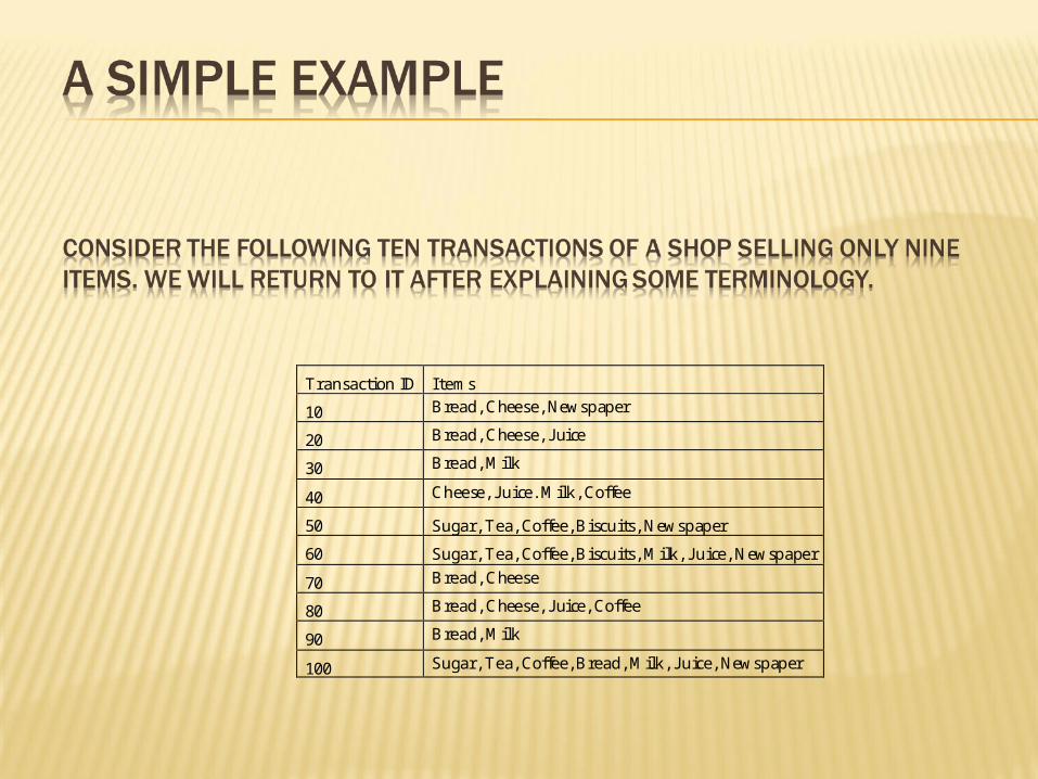
Suppose X and Y appear together in only 10% of the transactions but whenever X appears there is 80% chance that Y also appears.
The 10% presence of X and Y together is called the support (or prevalence) of the rule and 80% is called the confidence (or predictability) of the rule.
These are measures of interestingness of the rule.

• Confidence denotes the strength of the association between X and Y. Support indicates the frequency of the pattern. A minimum support is necessary if an association is going to be of some business value.
• Let the chance of finding an item X in the N transactions is x% then we can say probability of X is P(X) = x/100 since probability values are always between 0.0 and 1.0.
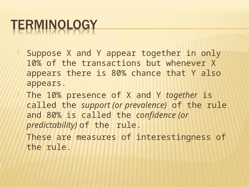
• Now suppose we have two items X and Y with probabilities of P(X) = 0.2 and P(Y) = 0.1. What does the product P(X) x P(Y) mean?
• What is likely to be the chance of both items X and Y appearing together, that is P(X and Y) = P(X U Y)?
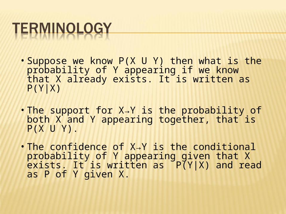
• Suppose we know P(X U Y) then what is the probability of Y appearing if we know that X already exists. It is written as P(Y|X)
• The support for X→Y is the probability of both X and Y appearing together, that is P(X U Y).
• The confidence of X→Y is the conditional probability of Y appearing given that X exists. It is written as P(Y|X) and read as P of Y given X.
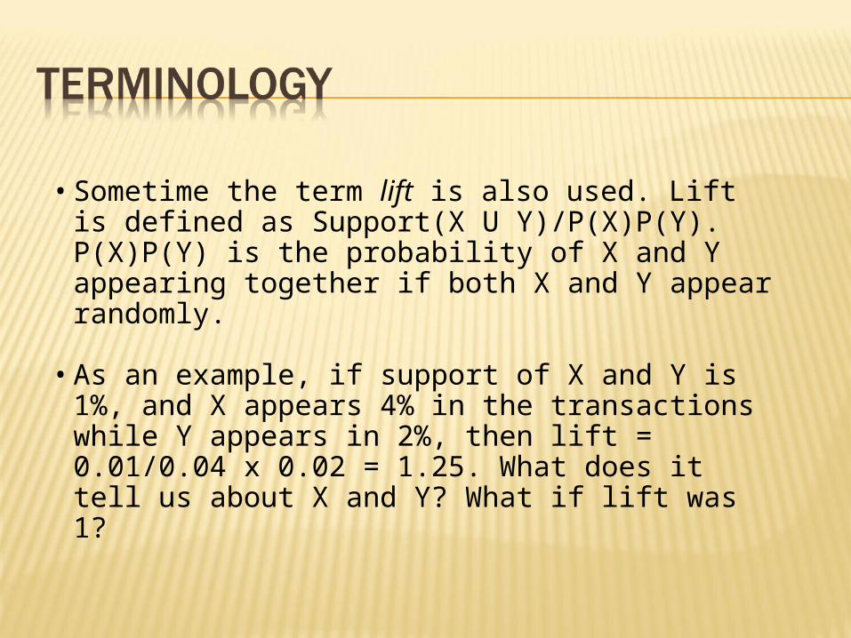
• Sometime the term lift is also used. Lift is defined as Support(X U Y)/P(X)P(Y). P(X)P(Y) is the probability of X and Y appearing together if both X and Y appear randomly.
• As an example, if support of X and Y is 1%, and X appears 4% in the transactions while Y appears in 2%, then lift = 0.01/0.04 x 0.02 = 1.25. What does it tell us about X and Y? What if lift was 1?

Want to find all associations which have at least p% support with at least q% confidence such that
all rules satisfying any user constraints are found
the rules are found efficiently from large databases
the rules found are actionable

example of n = 4 (Bread, Cheese, Juice, Milk) and N = 4. We want to find rules with minimum support of 50% and minimum confidence of 75%.
Transaction ID Items
100 Bread, Cheese
200 Bread, Cheese, J uice
300 Bread, Milk
400 Cheese, J uice. Milk

N = 4 results in the following frequencies. All items havethe 50% support we require. Only two pairshave the 50% supportand no 3-itemset hasthe support.
We will look at thetwo pairs that havethe minimum supportto find if they havethe required confidence.
Itemsets Frequency
Bread 3
Cheese 3
J uice 2
Milk 2
(Bread, Cheese) 2
(Bread, J uice) 1
(Bread, Milk) 1
(Cheese, J uice) 2
(Cheese, Milk) 1
(J uice, Milk) 1
(Bread, Cheese, J uice) 1
(Bread, Cheese, Milk) 0
(Bread, J uice, Milk) 0
(Cheese, J uice, Milk) 1
(Bread, Cheese, J uice, Milk) 0
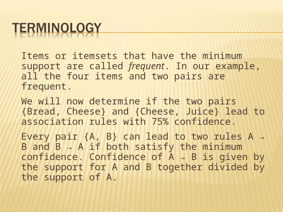
Items or itemsets that have the minimum support are called frequent. In our example, all the four items and two pairs are frequent.
We will now determine if the two pairs {Bread, Cheese} and {Cheese, Juice} lead to association rules with 75% confidence.
Every pair {A, B} can lead to two rules A → B and B → A if both satisfy the minimum confidence. Confidence of A → B is given by the support for A and B together divided by the support of A.

We have four possible rules and their confidence is given as follows:
Bread Cheese with confidence of 2/3 = 67%Cheese Bread with confidence of 2/3 = 67%Cheese Juice with confidence of 2/3 = 67%Juice Cheese with confidence of 100%
Therefore only the last rule Juice Cheese has confidence above the minimum 75% and qualifies. Rules that have more than user-specified minimum confidence are called confident.

This simple algorithm works well with four items since there were only a total of 16 combinations that we needed to look at but if the number of items is say 100, the number of combinations is much larger, in billions. The number of combinations becomes about a million with 20 items since the number of combinations is 2n with n items (why?). The naïve algorithm can be improved to deal more effectively with larger data sets.

Rather than counting all possible item combinations we can look at each transaction and count only the combinations that actually occur as shown below (that is, we don’t count itemsets with zero frequency).
Transaction ID Items Combinations 100 Bread, Cheese {Bread, Cheese} 200 Bread, Cheese,
J uice {Bread, Cheese}, {Bread, J uice}, {Cheese, J uice}, {Bread, Cheese, J uice}
300 Bread, Milk {Bread, Milk} 400 Cheese, J uice, Milk {Cheese, J uice}, {Cheese, Milk}, {J uice,
Milk}, {Cheese, J uice, Milk}

Itemsets Frequency Bread 3 Cheese 3 J uice 2 Milk 2 (Bread, Cheese) 2 (Bread, J uice) 1 (Bread, Milk) 1 (Cheese, J uice) 2 (J uice, Milk) 1 (Bread, Cheese, J uice) 1 (Cheese, J uice, Milk) 1
Removing zero frequencies leads to the smaller table below. We then proceed as before but the improvement is not large and we need better techniques.

To find associations, this classical Apriori algorithm may be simply described by a two step approach:
Step 1 ─ discover all frequent (single) items that have support above the minimum support required
Step 2 ─ use the set of frequent items to generate the association rules that have high enough confidence level

•A k-itemset is a set of k items.
•The set Ck is a set of candidate k-itemsets that are potentially frequent.
•The set Lk is a subset of Ck and is the set of k-itemsets that are frequent.

Step 1 – Computing L1
Scan all transactions. Find all frequent items that have support above the required p%. Let these frequent items be labeled L1.
Step 2 – Apriori-gen Function Use the frequent items L1 to build all possible item pairs like {Bread, Cheese} if Bread and Cheese are in L1. The set of these item pairs is called C2, the candidate set.
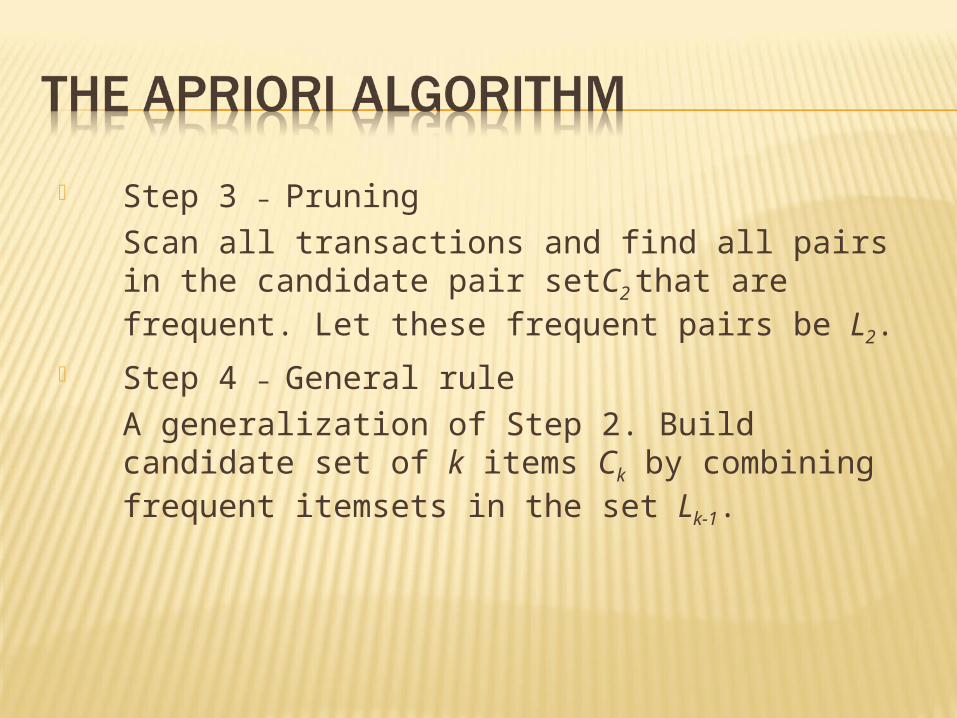
Step 3 – PruningScan all transactions and find all pairs in the candidate pair setC2 that are frequent. Let these frequent pairs be L2.
Step 4 – General rule A generalization of Step 2. Build candidate set of k items Ck by combining frequent itemsets in the set Lk-1.

Step 5 – PruningStep 5, generalization of Step 3. Scan all transactions and find all item sets in Ck that are frequent. Let these frequent itemsets be Lk.
Step 6 – ContinueContinue with Step 4 unless Lk is empty.
Step 7 – Stop Stop when Lk is empty.

Transaction ID Items 10 A, B, D 20 D, E, F 30 A, F 40 B, C, D 50 E, F 60 D, E, F 70 C, D, F 80 A, C, D, F
Consider only eight transactions with transaction IDs {10, 20, 30, 40, 50, 60, 70, 80}. This set of eight transactions with six items can be represented in at least three different ways as follows

TID A B C D E F 10 1 1 0 1 0 0 20 0 0 0 1 1 1 30 1 0 0 0 0 1 40 0 1 1 1 0 0 50 0 0 0 0 1 1 60 0 0 0 1 1 1 70 0 0 1 1 0 1 80 1 0 1 1 0 1
Consider only eight transactions with transaction IDs {10, 20, 30, 40, 50, 60, 70, 80}. This set of eight transactions with six items can be represented in at least three different ways as follows

Items 10 20 30 40 50 60 70 80 A 1 0 1 0 0 0 0 1 B 1 0 0 1 0 0 0 0 C 0 0 0 1 0 0 1 1 D 1 1 0 1 0 1 1 1 E 0 1 0 0 1 1 0 0 F 0 1 1 0 1 1 1 1
Consider only eight transactions with transaction IDs {10, 20, 30, 40, 50, 60, 70, 80}. This set of eight transactions with six items can be represented in at least three different ways as follows