
Introduction to Data Mining Using Weka
40
Introduction to Data Mining Using Weka Asst. Prof. Peerasak Intarapaiboon, Ph.D.
Transcript of Introduction to Data Mining Using Weka

Introduction to Data Mining Using Weka
Asst. Prof. Peerasak Intarapaiboon, Ph.D.
List of Topics
• Part-I: Introduction to data mining• Basic concepts
• Applications in the business’s world
• More details: tasks, learning algorithms, processes, etc.
• Some focused models
• Part-II: Quick tour in Weka• What is Weka?
• How to install Weka
• Fundamental tools in Weka
• Let’s start to use Weka
Workshop@TU 2

Workshop@TU 3

Applications of DM: Where are you?
Workshop@TU 4

Applications of DM: Where are you?
Workshop@TU 5
RecommendationSystems

Applications of DM: Where are you?
Workshop@TU 6
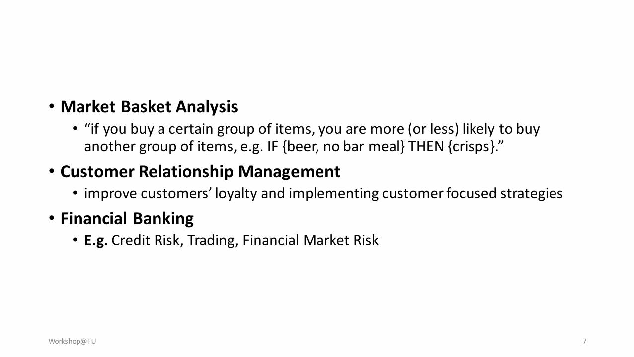
• Market Basket Analysis• “if you buy a certain group of items, you are more (or less) likely to buy
another group of items, e.g. IF {beer, no bar meal} THEN {crisps}.”
• Customer Relationship Management• improve customers’ loyalty and implementing customer focused strategies
• Financial Banking• E.g. Credit Risk, Trading, Financial Market Risk
Workshop@TU 7
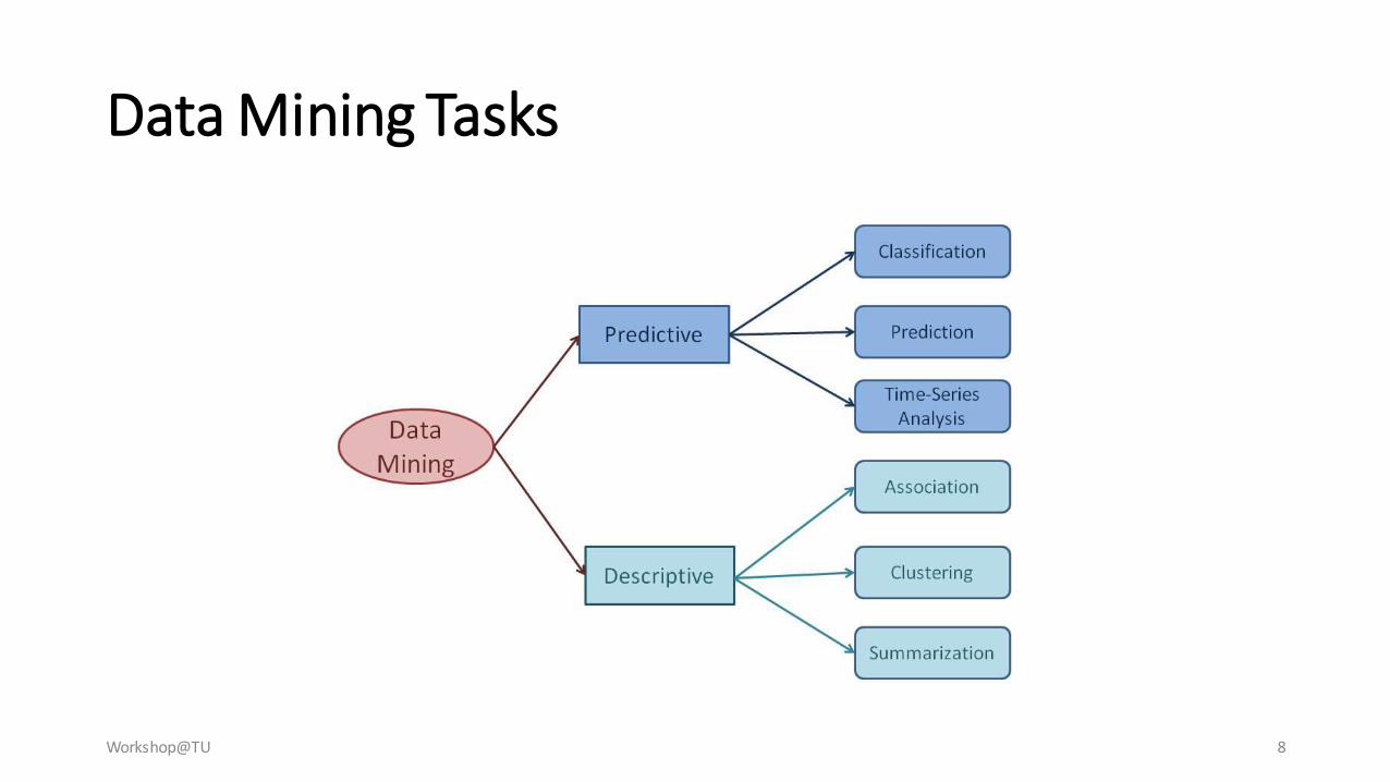
Data Mining Tasks
Workshop@TU 8
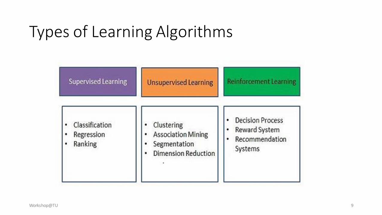
Types of Learning Algorithms
Workshop@TU 9
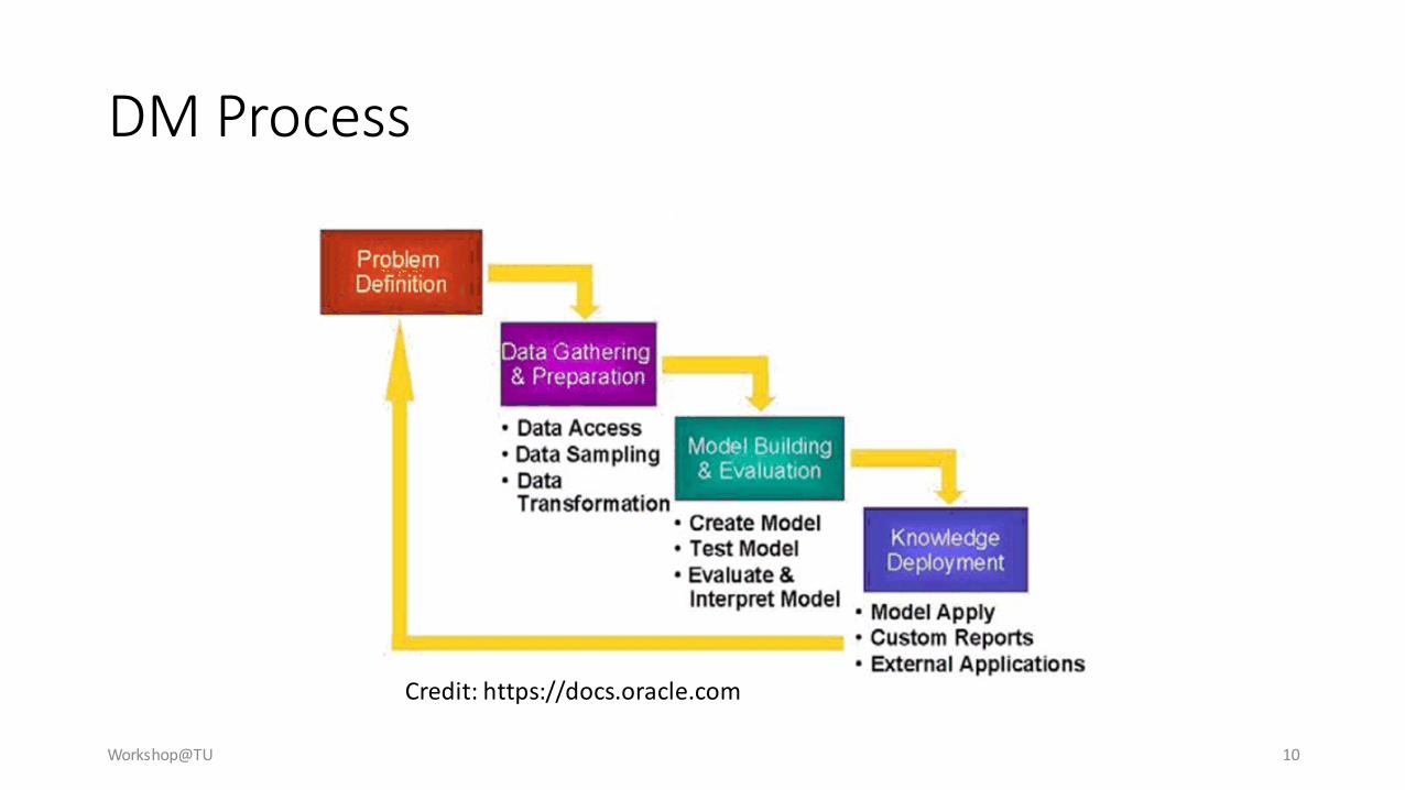
DM Process
Workshop@TU 10
Credit: https://docs.oracle.com

Workshop@TU 11
• Classification by decision tree induction
• Bayesian classification
• Rule-based classification
• Classification by back propagation
• Support Vector Machines (SVM)
• Associative classification
• Lazy learners (or learning from your neighbors)
Classification

Workshop@TU 12
age income student credit_rating buys_computer
<=30 high no fair no
<=30 high no excellent no
31…40 high no fair yes
>40 medium no fair yes
>40 low yes fair yes
>40 low yes excellent no
31…40 low yes excellent yes
<=30 medium no fair no
<=30 low yes fair yes
>40 medium yes fair yes
<=30 medium yes excellent yes
31…40 medium no excellent yes
31…40 high yes fair yes
>40 medium no excellent no
1. Classification: Decision Tree
Workshop@TU 13
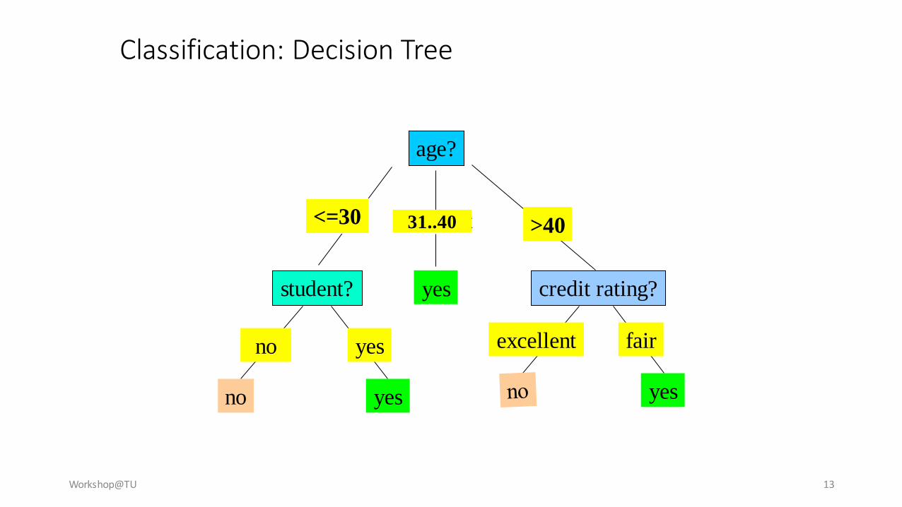
Classification: Decision Tree
age?
overcast
student? credit rating?
<=30 >40
no yes yes
yes
31..40
fairexcellentyesno

Workshop@TU 14
X1 X2 Class
1 1 Yes
1 2 Yes
1 2 Yes
1 2 Yes
1 2 Yes
1 1 No
2 1 No
2 1 No
2 2 No
2 2 No
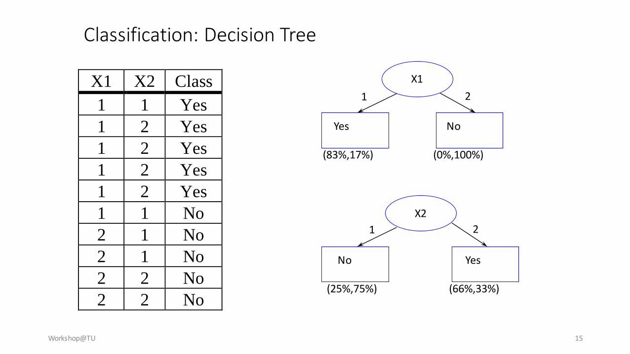
Classification: Decision Tree
Workshop@TU 15
X1 X2 Class
1 1 Yes
1 2 Yes
1 2 Yes
1 2 Yes
1 2 Yes
1 1 No
2 1 No
2 1 No
2 2 No
2 2 No
X1
X2
Yes
(83%,17%)
No
(25%,75%)
No
(0%,100%)
Yes
(66%,33%)
Classification: Decision Tree
1 2
1 2

Workshop@TU 16
Select the attribute with the highest information gain
Let pi be the probability that an arbitrary tuple in D belongs to class Ci, estimated by |Ci, D|/|D|
Expected information (entropy) needed to classify a tuple
in D:
Information needed (after using A to split D into v partitions) to classify D:
Information gained by branching on attribute A
)(log)( 2
1
i
m
i
i ppDInfo
1
| |( ) ( )
| |
vj
A j
j
DInfo D Info D
D
(D)InfoInfo(D)Gain(A) A
Attribute Measurements
Workshop 1
• Create a decision tree from “ComPurchase.csv” and “TicTacToe.csv”
• Explore the weka environment• Data loading
• Data information
• Model learning
• Model evaluation
Workshop@TU 17
Workshop@TU 18
Discretization
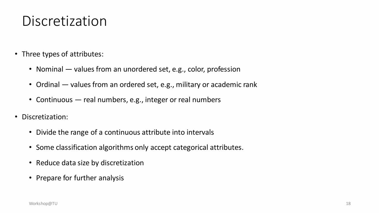
• Three types of attributes:
• Nominal — values from an unordered set, e.g., color, profession
• Ordinal — values from an ordered set, e.g., military or academic rank
• Continuous — real numbers, e.g., integer or real numbers
• Discretization:
• Divide the range of a continuous attribute into intervals
• Some classification algorithms only accept categorical attributes.
• Reduce data size by discretization
• Prepare for further analysis
Workshop@TU 19
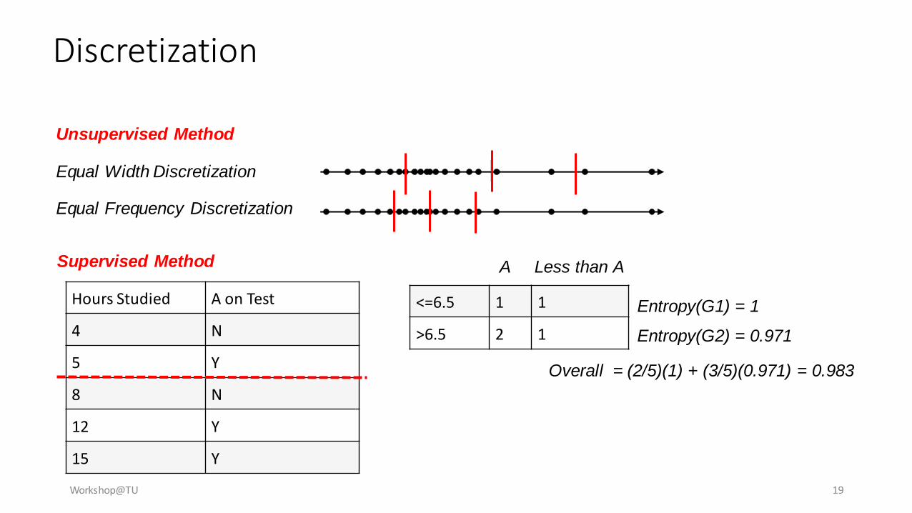
Unsupervised Method
Equal Frequency Discretization
Discretization
Equal Width Discretization
Supervised Method
Hours Studied A on Test
4 N
5 Y
8 N
12 Y
15 Y
<=6.5 1 1
>6.5 2 1
A Less than A
Entropy(G1) = 1
Entropy(G2) = 0.971
Overall = (2/5)(1) + (3/5)(0.971) = 0.983

Workshop 2
• How to handle numeric attributes• Discretization
• Use “Iris.csv”
• Data type• Use “Car.csv”
Workshop@TU 20
Workshop@TU 21
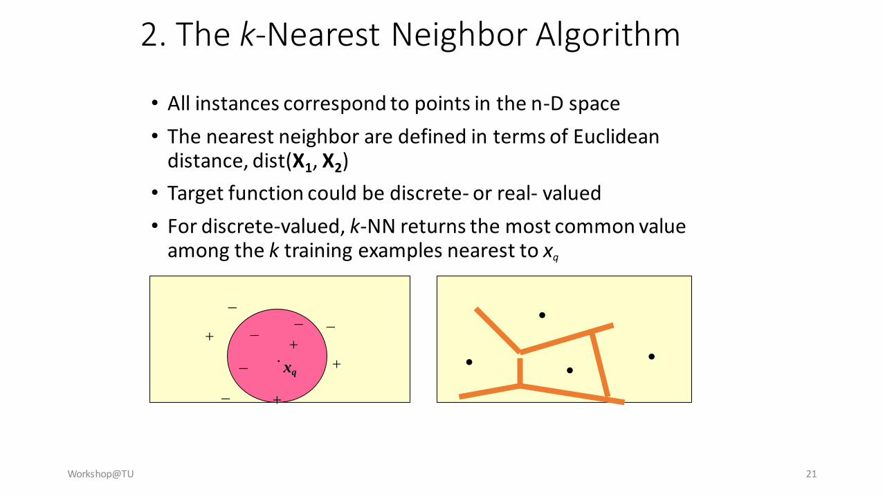
2. The k-Nearest Neighbor Algorithm
• All instances correspond to points in the n-D space
• The nearest neighbor are defined in terms of Euclidean distance, dist(X1, X2)
• Target function could be discrete- or real- valued
• For discrete-valued, k-NN returns the most common value among the k training examples nearest to xq
.
_+
_ xq
+
_ _+
_
_
+
.
.. .

Workshop 3
• Apply kNN to “Iris.csv”
• Compare with the results in Workshop 2
Workshop@TU 22
Workshop@TU 23
3. Bayesian Classification• A statistical classifier: performs probabilistic prediction, i.e.,
predicts class membership probabilities
• Foundation: Based on Bayes’ Theorem.
• Performance: A simple Bayesian classifier, naïve Bayesian classifier, has comparable performance with decision tree and selected neural network classifiers
• Incremental: Each training example can incrementally increase/decrease the probability that a hypothesis is correct —prior knowledge can be combined with observed data
• Standard: Even when Bayesian methods are computationally intractable, they can provide a standard of optimal decision making against which other methods can be measured
Workshop@TU 24
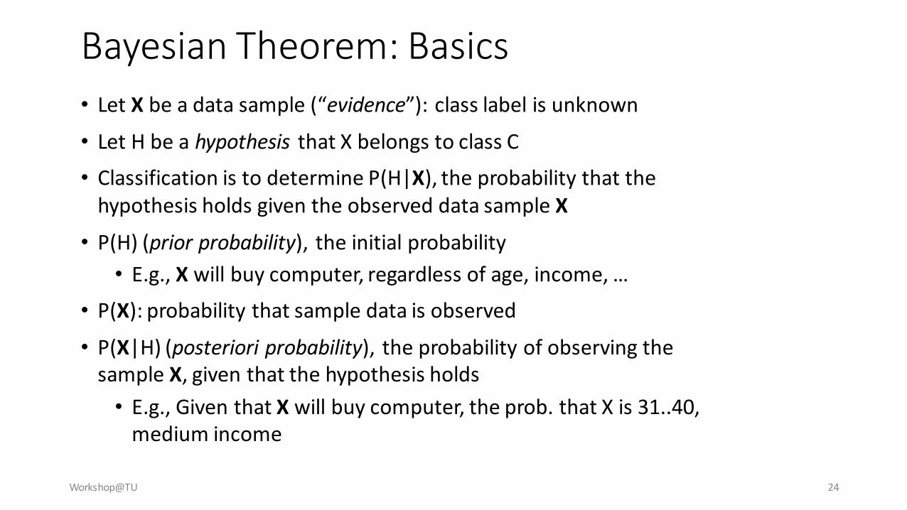
Bayesian Theorem: Basics
• Let X be a data sample (“evidence”): class label is unknown
• Let H be a hypothesis that X belongs to class C
• Classification is to determine P(H|X), the probability that the hypothesis holds given the observed data sample X
• P(H) (prior probability), the initial probability
• E.g., X will buy computer, regardless of age, income, …
• P(X): probability that sample data is observed
• P(X|H) (posteriori probability), the probability of observing the sample X, given that the hypothesis holds
• E.g., Given that X will buy computer, the prob. that X is 31..40, medium income

Workshop@TU 25
Bayesian Theorem
• Given training data X, posteriori probability of a hypothesis H,
P(H|X), follows the Bayes theorem
• Informally, this can be written as
posteriori = likelihood x prior/evidence
• Predicts X belongs to C2 iff the probability P(Ci|X) is the highest
among all the P(Ck|X) for all the k classes
• Practical difficulty: require initial knowledge of many
probabilities, significant computational cost
)()()|()|(
XXX
PHPHPHP
Workshop@TU 26
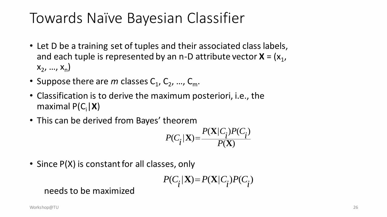
Towards Naïve Bayesian Classifier
• Let D be a training set of tuples and their associated class labels, and each tuple is represented by an n-D attribute vector X = (x1, x2, …, xn)
• Suppose there are m classes C1, C2, …, Cm.
• Classification is to derive the maximum posteriori, i.e., the maximal P(Ci|X)
• This can be derived from Bayes’ theorem
• Since P(X) is constant for all classes, only
needs to be maximized
)(
)()|()|(
X
XX
Pi
CPi
CP
iCP
)()|()|(i
CPi
CPi
CP XX
Workshop@TU 27
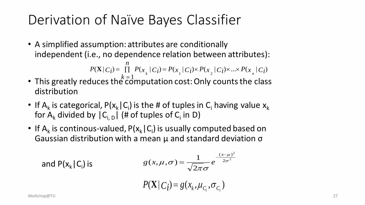
Derivation of Naïve Bayes Classifier
• A simplified assumption: attributes are conditionally independent (i.e., no dependence relation between attributes):
• This greatly reduces the computation cost: Only counts the class distribution
• If Ak is categorical, P(xk|Ci) is the # of tuples in Ci having value xk
for Ak divided by |Ci, D| (# of tuples of Ci in D)
• If Ak is continous-valued, P(xk|Ci) is usually computed based on Gaussian distribution with a mean μ and standard deviation σ
and P(xk|Ci) is
)|(...)|()|(
1
)|()|(21
CixPCixPCixPn
kCixPCiP
nk
X
2
2
2
)(
2
1),,(
x
exg
),,()|(ii CCkxgCiP X
Workshop@TU 28
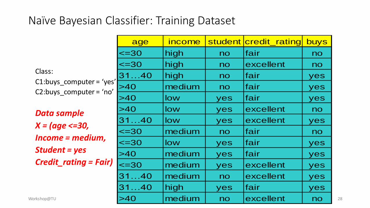
Naïve Bayesian Classifier: Training Dataset
Class:
C1:buys_computer = ‘yes’
C2:buys_computer = ‘no’
Data sample
X = (age <=30,
Income = medium,
Student = yes
Credit_rating = Fair)
age income student credit_rating buys
<=30 high no fair no
<=30 high no excellent no
31…40 high no fair yes
>40 medium no fair yes
>40 low yes fair yes
>40 low yes excellent no
31…40 low yes excellent yes
<=30 medium no fair no
<=30 low yes fair yes
>40 medium yes fair yes
<=30 medium yes excellent yes
31…40 medium no excellent yes
31…40 high yes fair yes
>40 medium no excellent no
Workshop@TU 29
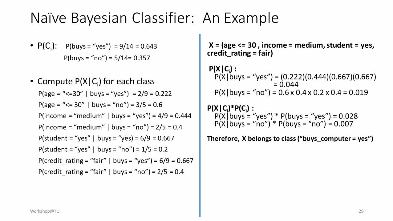
Naïve Bayesian Classifier: An Example
• P(Ci): P(buys = “yes”) = 9/14 = 0.643
P(buys = “no”) = 5/14= 0.357
• Compute P(X|Ci) for each classP(age = “<=30” | buys = “yes”) = 2/9 = 0.222
P(age = “<= 30” | buys = “no”) = 3/5 = 0.6
P(income = “medium” | buys = “yes”) = 4/9 = 0.444
P(income = “medium” | buys = “no”) = 2/5 = 0.4
P(student = “yes” | buys = “yes) = 6/9 = 0.667
P(student = “yes” | buys = “no”) = 1/5 = 0.2
P(credit_rating = “fair” | buys = “yes”) = 6/9 = 0.667
P(credit_rating = “fair” | buys = “no”) = 2/5 = 0.4
X = (age <= 30 , income = medium, student = yes, credit_rating = fair)
P(X|Ci) :P(X|buys = “yes”) = (0.222)(0.444)(0.667)(0.667)
= 0.044P(X|buys = “no”) = 0.6 x 0.4 x 0.2 x 0.4 = 0.019
P(X|Ci)*P(Ci) :P(X|buys = “yes”) * P(buys = “yes”) = 0.028 P(X|buys = “no”) * P(buys = “no”) = 0.007
Therefore, X belongs to class (“buys_computer = yes”)
Workshop 4
• Apply Naïve Bayes to the previous datasets
Workshop@TU 30
Workshop@TU 31
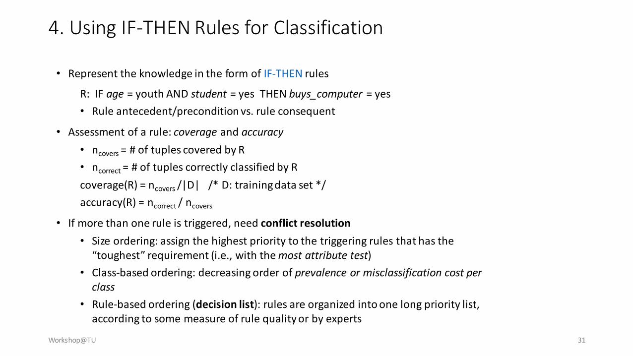
4. Using IF-THEN Rules for Classification
• Represent the knowledge in the form of IF-THEN rules
R: IF age = youth AND student = yes THEN buys_computer = yes
• Rule antecedent/precondition vs. rule consequent
• Assessment of a rule: coverage and accuracy
• ncovers = # of tuples covered by R
• ncorrect = # of tuples correctly classified by R
coverage(R) = ncovers /|D| /* D: training data set */
accuracy(R) = ncorrect / ncovers
• If more than one rule is triggered, need conflict resolution
• Size ordering: assign the highest priority to the triggering rules that has the “toughest” requirement (i.e., with the most attribute test)
• Class-based ordering: decreasing order of prevalence or misclassification cost per class
• Rule-based ordering (decision list): rules are organized into one long priority list, according to some measure of rule quality or by experts

Workshop@TU 32
age?
student? credit rating?
<=30 >40
no yes yes
yes
31..40
fairexcellentyesno
• Example: Rule extraction from our buys_computer decision-tree
IF age = young AND student = no THEN buys_computer = no
IF age = young AND student = yes THEN buys_computer = yes
IF age = mid-age THEN buys_computer = yes
IF age = old AND credit_rating = excellent THEN buys_computer = yes
IF age = young AND credit_rating = fair THEN buys_computer = no
Rule Extraction from a Decision Tree
Rules are easier to understand than large trees
One rule is created for each path from the root
to a leaf
Each attribute-value pair along a path forms a
conjunction: the leaf holds the class prediction
Rules are mutually exclusive and exhaustive

Workshop@TU 33
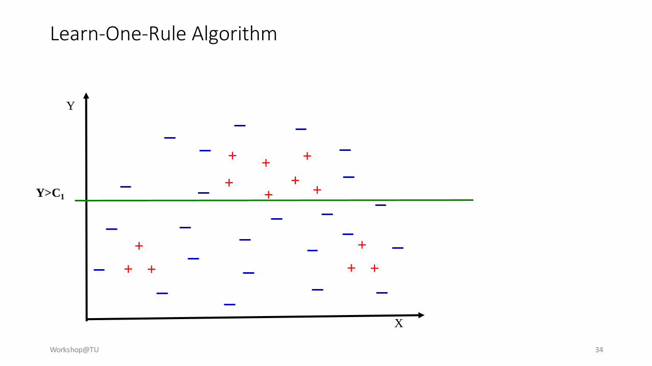
Learn-One-Rule Algorithm
X
Y
+ +
++
+
+
+
+ +
+
+ +
+
Workshop@TU 34
X
Y
+ +
++
+
+
+
+ +
+
+ +
+Y>C1
Learn-One-Rule Algorithm
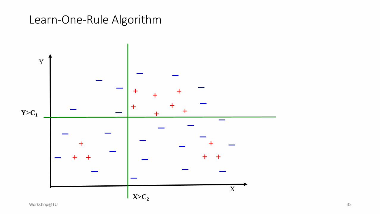
Workshop@TU 35
X
Y
+ +
++
+
+
+
+ +
+
+ +
+Y>C1
X>C2
Learn-One-Rule Algorithm
Workshop@TU 3627
X
Y
+ +
++
+
+
+
+ +
+
+ +
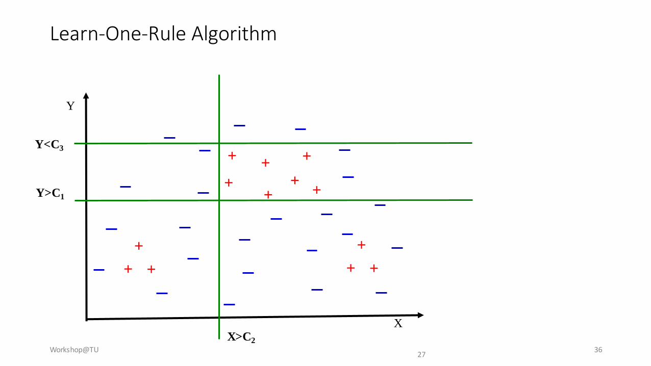
+Y>C1
X>C2
Y<C3
Learn-One-Rule Algorithm
Workshop@TU 37
X
Y
+ +
++
+
+
+
+ +
+
+ +
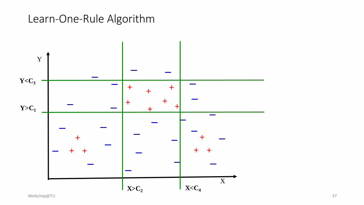
+Y>C1
X>C2
Y<C3
X<C4
Learn-One-Rule Algorithm
Workshop@TU 38
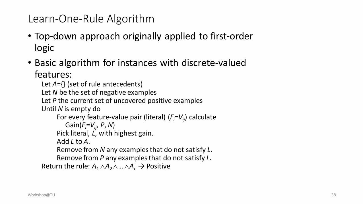
• Top-down approach originally applied to first-order logic
• Basic algorithm for instances with discrete-valued features:
Let A={} (set of rule antecedents)Let N be the set of negative examplesLet P the current set of uncovered positive examplesUntil N is empty do
For every feature-value pair (literal) (Fi=Vij) calculateGain(Fi=Vij, P, N)
Pick literal, L, with highest gain.Add L to A.Remove from N any examples that do not satisfy L.Remove from P any examples that do not satisfy L.
Return the rule: A1 A2 … An → Positive
Learn-One-Rule Algorithm
Workshop@TU 3941
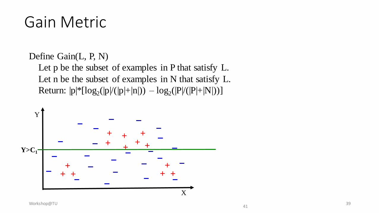
Gain Metric
Define Gain(L, P, N)
Let p be the subset of examples in P that satisfy L.
Let n be the subset of examples in N that satisfy L.
Return: |p|*[log2(|p|/(|p|+|n|)) – log2(|P|/(|P|+|N|))]
X
Y
+ +++
+
+
++ +
++ +
+Y>C1
Workshop 5
• Apply rule learner algorithms to the previous datasetsCompare results from datasets with/without discretization
Workshop@TU 40


![A Comparison of Data Mining Tools using the … Weka Tool Weka [11] is an open source tool for the implementation of various data mining algorithms. It is based on java application](https://static.fdocuments.us/doc/165x107/5acf2b167f8b9ad24f8c1c52/a-comparison-of-data-mining-tools-using-the-weka-tool-weka-11-is-an-open-source.jpg)