Introduction to Curve Estimationcompdiag.molgen.mpg.de/docs/curve_estimation.pdf · Stefanie Scheid...
41
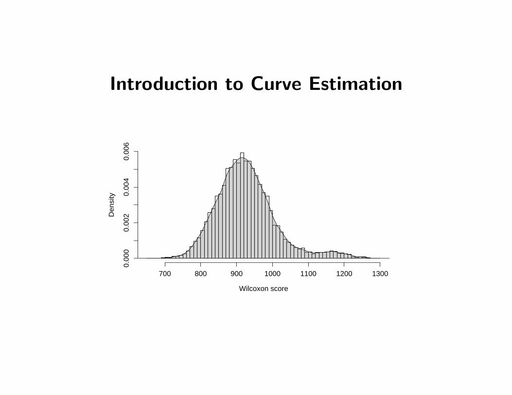
Introduction to Curve Estimation Wilcoxon score Density 700 800 900 1000 1100 1200 1300 0.000 0.002 0.004 0.006
Transcript of Introduction to Curve Estimationcompdiag.molgen.mpg.de/docs/curve_estimation.pdf · Stefanie Scheid...
Introduction to Curve Estimation
Wilcoxon score
Den
sity
700 800 900 1000 1100 1200 1300
0.00
00.
002
0.00
40.
006
Michael E. Tarter & Micheal D. Lock
Model-Free Curve Estimation
Monographs on Statistics and Applied Probability 56
Chapman & Hall, 1993.
Chapters 1–4.
Stefanie Scheid - Introduction to Curve Estimation - August 11, 2003 1
Outline
1. Generalized representation
2. Short review on Fourier series
3. Fourier series density estimation
4. Kernel density estimation
5. Optimizing density estimates
Stefanie Scheid - Introduction to Curve Estimation - August 11, 2003 2
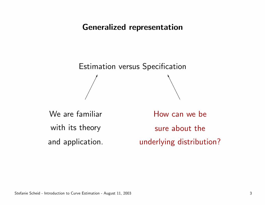
Generalized representation
Estimation versus Specification
���������
We are familiar
with its theory
and application.
AAAAAAAAK
How can we be
sure about the
underlying distribution?
Stefanie Scheid - Introduction to Curve Estimation - August 11, 2003 3
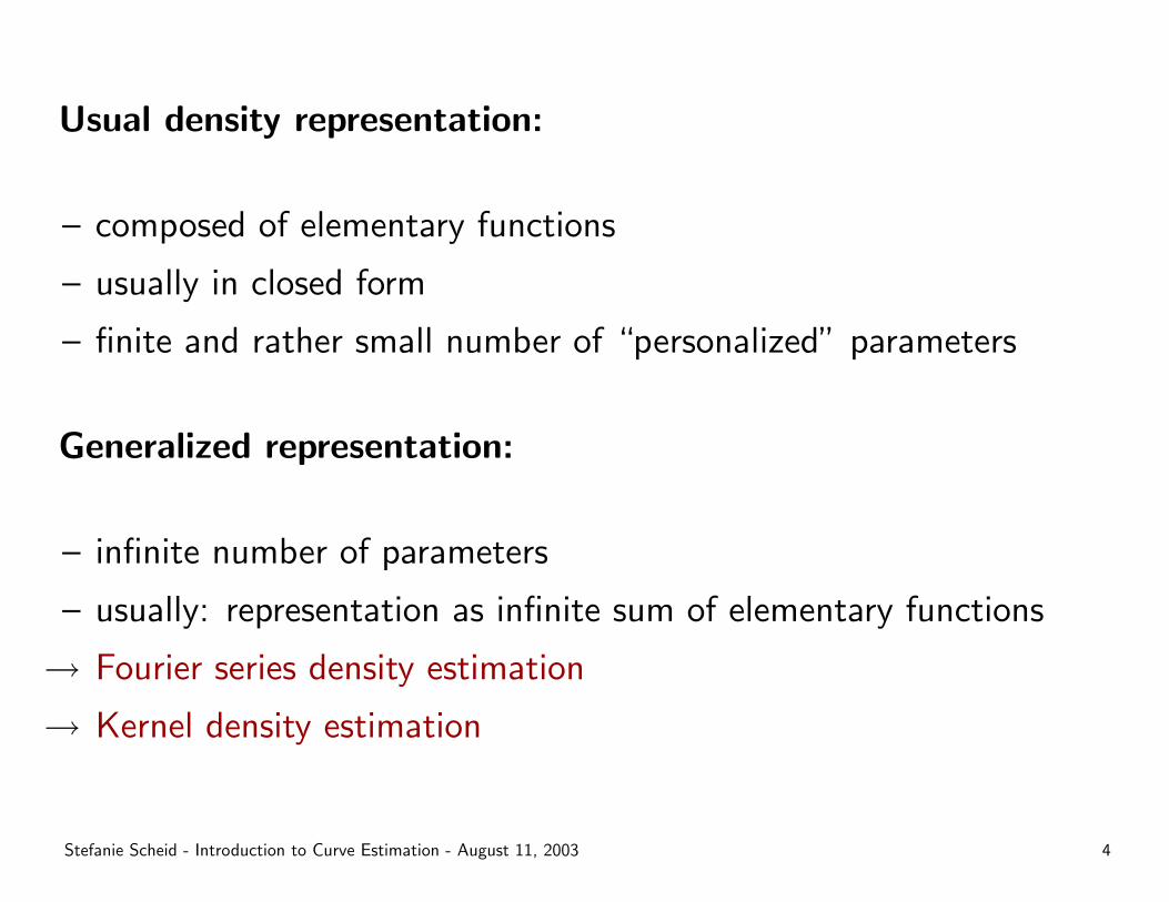
Usual density representation:
– composed of elementary functions
– usually in closed form
– finite and rather small number of “personalized” parameters
Generalized representation:
– infinite number of parameters
– usually: representation as infinite sum of elementary functions
→ Fourier series density estimation
→ Kernel density estimation
Stefanie Scheid - Introduction to Curve Estimation - August 11, 2003 4
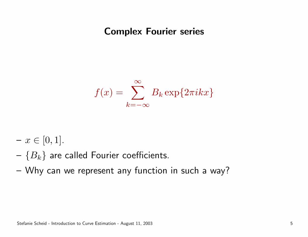
Complex Fourier series
f(x) =∞∑
k=−∞
Bk exp{2πikx}
– x ∈ [0, 1].
– {Bk} are called Fourier coefficients.
– Why can we represent any function in such a way?
Stefanie Scheid - Introduction to Curve Estimation - August 11, 2003 5
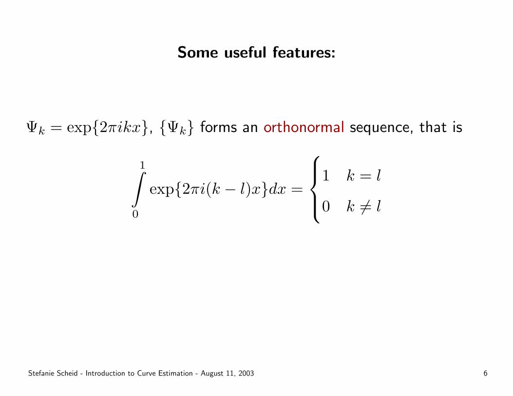
Some useful features:
Ψk = exp{2πikx}, {Ψk} forms an orthonormal sequence, that is
1∫0
exp{2πi(k − l)x}dx =
1 k = l
0 k 6= l
Stefanie Scheid - Introduction to Curve Estimation - August 11, 2003 6
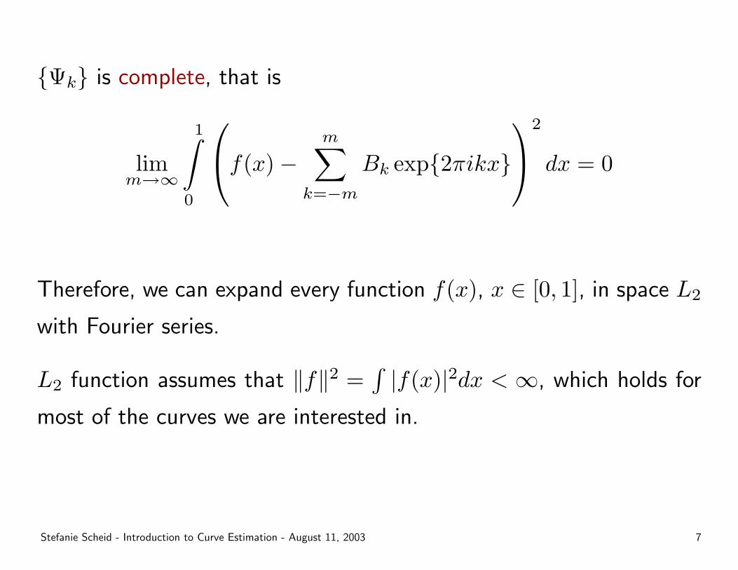
{Ψk} is complete, that is
limm→∞
1∫0
f(x)−m∑
k=−m
Bk exp{2πikx}
2
dx = 0
Therefore, we can expand every function f(x), x ∈ [0, 1], in space L2
with Fourier series.
L2 function assumes that ‖f‖2 =∫|f(x)|2dx < ∞, which holds for
most of the curves we are interested in.
Stefanie Scheid - Introduction to Curve Estimation - August 11, 2003 7
Fourier series density estimation
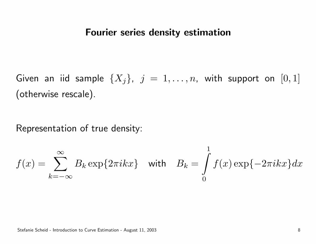
Given an iid sample {Xj}, j = 1, . . . , n, with support on [0, 1]
(otherwise rescale).
Representation of true density:
f(x) =∞∑
k=−∞
Bk exp{2πikx} with Bk =
1∫0
f(x) exp{−2πikx}dx
Stefanie Scheid - Introduction to Curve Estimation - August 11, 2003 8
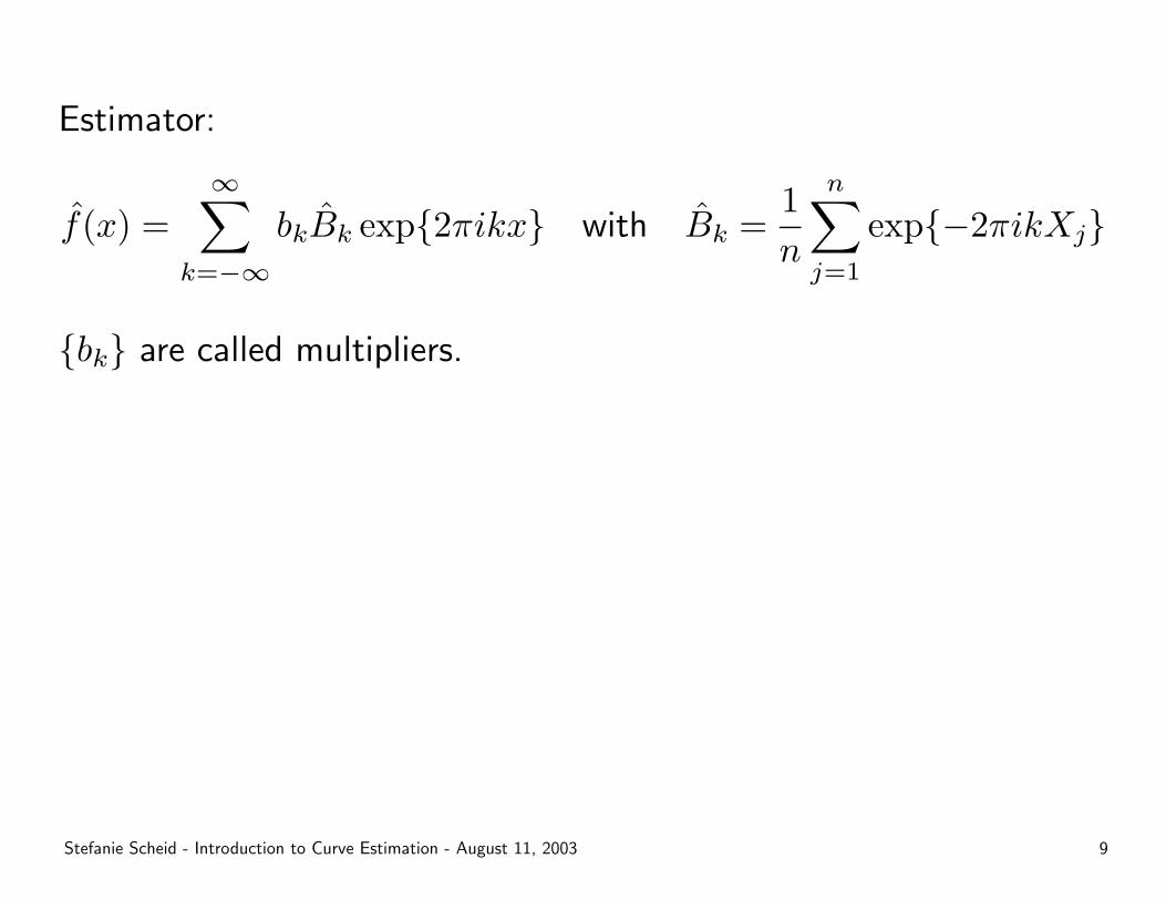
Estimator:
f̂(x) =∞∑
k=−∞
bkB̂k exp{2πikx} with B̂k =1n
n∑j=1
exp{−2πikXj}
{bk} are called multipliers.
Stefanie Scheid - Introduction to Curve Estimation - August 11, 2003 9
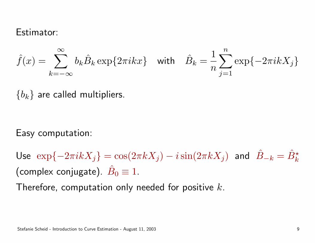
Estimator:
f̂(x) =∞∑
k=−∞
bkB̂k exp{2πikx} with B̂k =1n
n∑j=1
exp{−2πikXj}
{bk} are called multipliers.
Easy computation:
Use exp{−2πikXj} = cos(2πkXj)− i sin(2πkXj) and B̂−k = B̂?k
(complex conjugate). B̂0 ≡ 1.
Therefore, computation only needed for positive k.
Stefanie Scheid - Introduction to Curve Estimation - August 11, 2003 9
B̂k is unbiased estimator for Bk.
However, f̂ is usually biased because number of terms is either infinite
or unknown.
Another advantage of sample coefficients {B̂k}: Same set leads to
variety of other estimates.
That’s where multipliers come into play!
Stefanie Scheid - Introduction to Curve Estimation - August 11, 2003 10
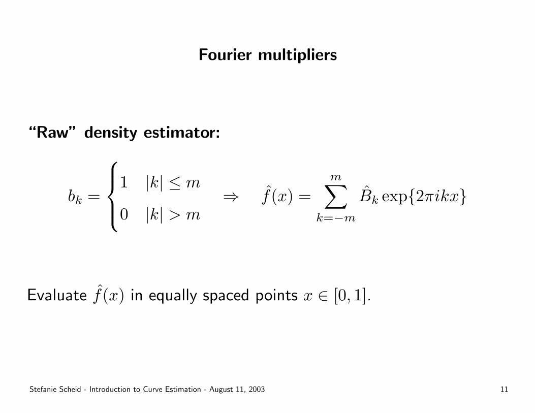
Fourier multipliers
“Raw” density estimator:
bk =
1 |k| ≤ m
0 |k| > m⇒ f̂(x) =
m∑k=−m
B̂k exp{2πikx}
Evaluate f̂(x) in equally spaced points x ∈ [0, 1].
Stefanie Scheid - Introduction to Curve Estimation - August 11, 2003 11
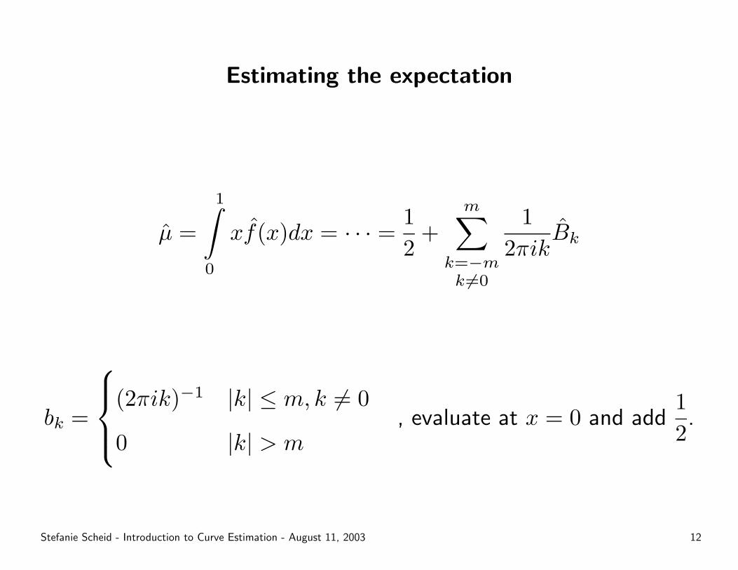
Estimating the expectation
µ̂ =
1∫0
xf̂(x)dx = · · · = 12
+m∑
k=−mk 6=0
12πik
B̂k
bk =
(2πik)−1 |k| ≤ m, k 6= 0
0 |k| > m, evaluate at x = 0 and add
12
.
Stefanie Scheid - Introduction to Curve Estimation - August 11, 2003 12
Advantages of multipliers
– Examination of various distributional features without recomputing
sample coefficients.
– Optimize the estimation procedure.
– Smoothing of estimated curve vs. higher contrast.
Some examples . . .
Stefanie Scheid - Introduction to Curve Estimation - August 11, 2003 13
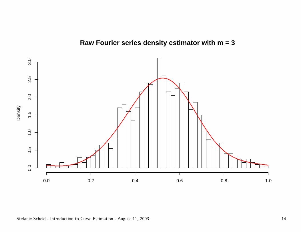
Raw Fourier series density estimator with m = 3
Den
sity
0.0 0.2 0.4 0.6 0.8 1.0
0.0
0.5
1.0
1.5
2.0
2.5
3.0
Stefanie Scheid - Introduction to Curve Estimation - August 11, 2003 14
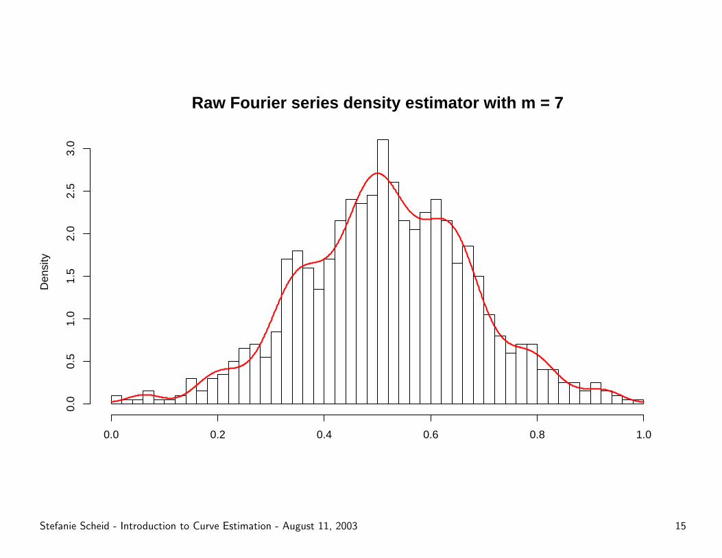
Raw Fourier series density estimator with m = 7
Den
sity
0.0 0.2 0.4 0.6 0.8 1.0
0.0
0.5
1.0
1.5
2.0
2.5
3.0
Stefanie Scheid - Introduction to Curve Estimation - August 11, 2003 15
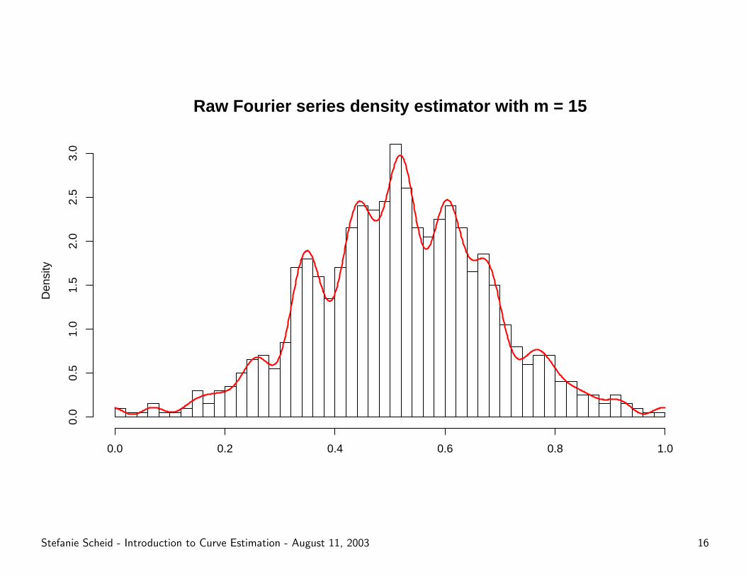
Raw Fourier series density estimator with m = 15
Den
sity
0.0 0.2 0.4 0.6 0.8 1.0
0.0
0.5
1.0
1.5
2.0
2.5
3.0
Stefanie Scheid - Introduction to Curve Estimation - August 11, 2003 16
Kernel density estimation
Histograms are crude kernel density estimators where the kernel is a
block (rectangular shape) somehow positioned over a data point.
Stefanie Scheid - Introduction to Curve Estimation - August 11, 2003 17
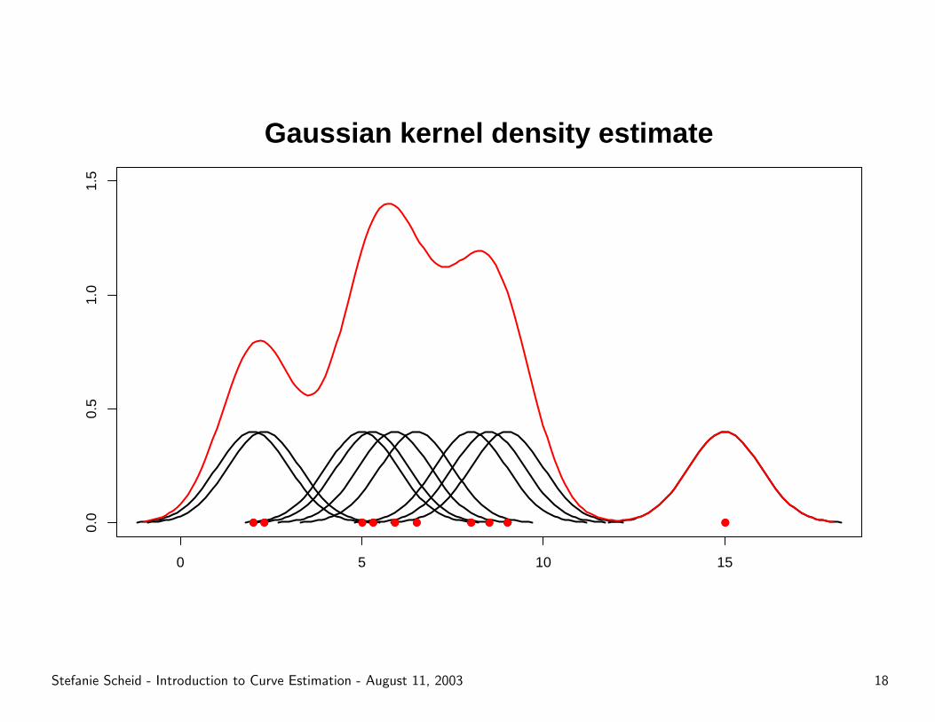
Kernel density estimation
Histograms are crude kernel density estimators where the kernel is a
block (rectangular shape) somehow positioned over a data point.
Kernel estimators:
– use various shapes as kernels
– place the center of a kernel right over the data point
– spread the influence of one point with varying kernel width
⇒ contribution from each kernel is summed to overall estimate
Stefanie Scheid - Introduction to Curve Estimation - August 11, 2003 17
● ● ● ● ● ● ● ● ● ●
0 5 10 15
0.0
0.5
1.0
1.5
Gaussian kernel density estimate
● ● ● ● ● ● ● ● ● ●
Stefanie Scheid - Introduction to Curve Estimation - August 11, 2003 18
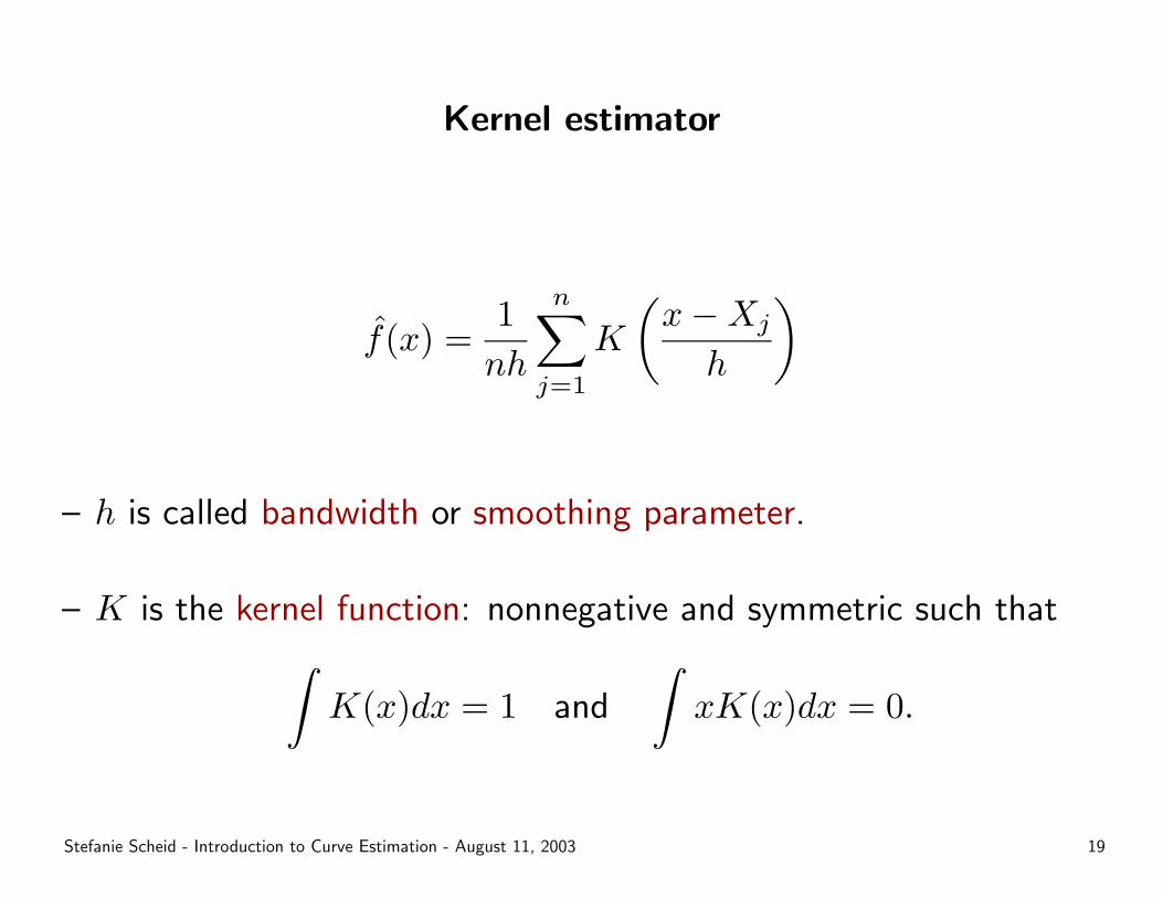
Kernel estimator
f̂(x) =1nh
n∑j=1
K
(x−Xj
h
)
– h is called bandwidth or smoothing parameter.
– K is the kernel function: nonnegative and symmetric such that∫K(x)dx = 1 and
∫xK(x)dx = 0.
Stefanie Scheid - Introduction to Curve Estimation - August 11, 2003 19
– Under mild conditions (h must decrease with increasing n) the
kernel estimate converges in probability to the true density.
– Choice of kernel function usually depends on computational criteria.
– Choice of bandwidth is more important (see literature on “Kernel
Smoothing”).
Stefanie Scheid - Introduction to Curve Estimation - August 11, 2003 20
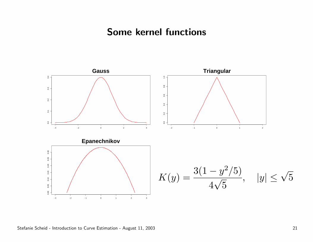
Some kernel functions
−4 −2 0 2 4
0.0
0.1
0.2
0.3
0.4
Gauss
−2 −1 0 1 2
0.0
0.2
0.4
0.6
0.8
1.0
Triangular
−3 −2 −1 0 1 2 3
0.00
0.05
0.10
0.15
0.20
0.25
0.30
Epanechnikov
K(y) =3(1− y2/5)
4√
5, |y| ≤
√5
Stefanie Scheid - Introduction to Curve Estimation - August 11, 2003 21
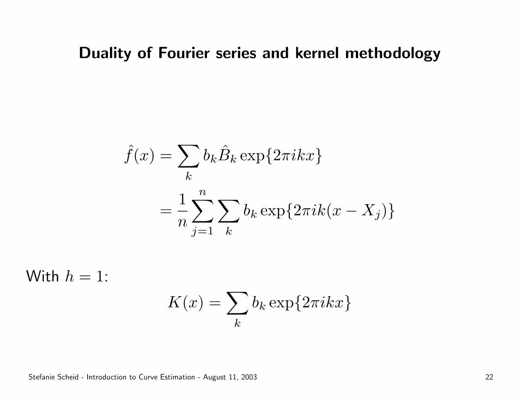
Duality of Fourier series and kernel methodology
f̂(x) =∑k
bkB̂k exp{2πikx}
=1n
n∑j=1
∑k
bk exp{2πik(x−Xj)}
With h = 1:
K(x) =∑k
bk exp{2πikx}
Stefanie Scheid - Introduction to Curve Estimation - August 11, 2003 22
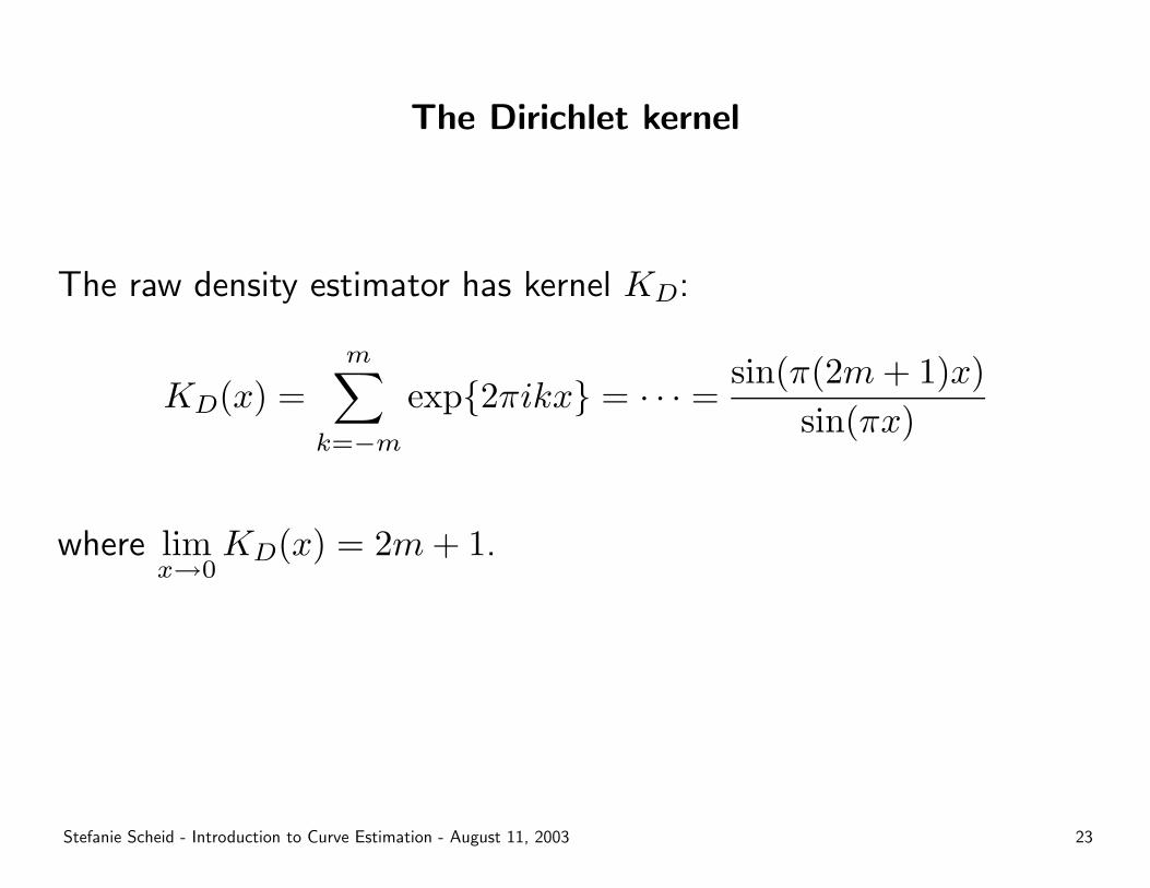
The Dirichlet kernel
The raw density estimator has kernel KD:
KD(x) =m∑
k=−m
exp{2πikx} = · · · = sin(π(2m+ 1)x)sin(πx)
where limx→0
KD(x) = 2m+ 1.
Stefanie Scheid - Introduction to Curve Estimation - August 11, 2003 23
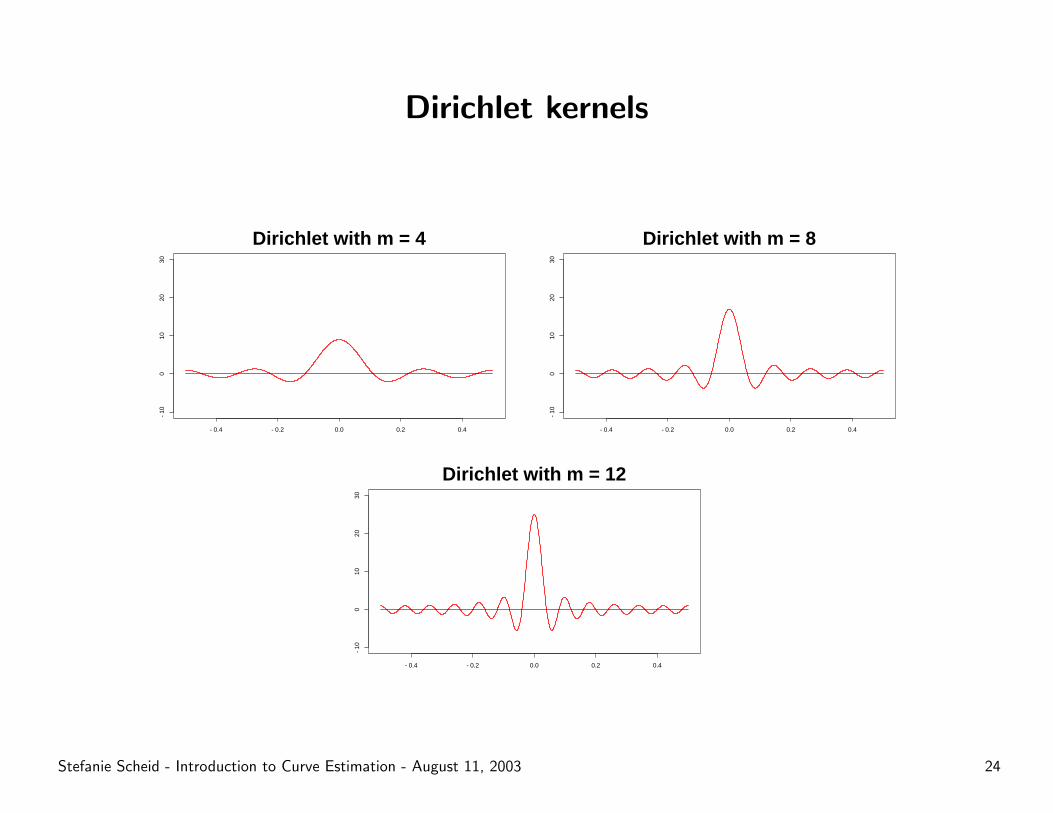
Dirichlet kernels
−0.4 −0.2 0.0 0.2 0.4
−10
010
2030
Dirichlet with m = 4
−0.4 −0.2 0.0 0.2 0.4
−10
010
2030
Dirichlet with m = 8
−0.4 −0.2 0.0 0.2 0.4
−10
010
2030
Dirichlet with m = 12
Stefanie Scheid - Introduction to Curve Estimation - August 11, 2003 24
Differences between kernel and Fourier representation
– Fourier estimates are restricted to finite intervals while some kernels
are not.
– As Dirichlet kernel shows, kernel estimates can result in negative
values if the kernel function takes on negative values.
Stefanie Scheid - Introduction to Curve Estimation - August 11, 2003 25
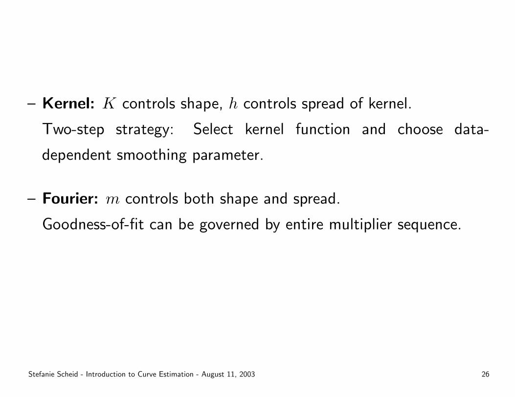
– Kernel: K controls shape, h controls spread of kernel.
Two-step strategy: Select kernel function and choose data-
dependent smoothing parameter.
– Fourier: m controls both shape and spread.
Goodness-of-fit can be governed by entire multiplier sequence.
Stefanie Scheid - Introduction to Curve Estimation - August 11, 2003 26
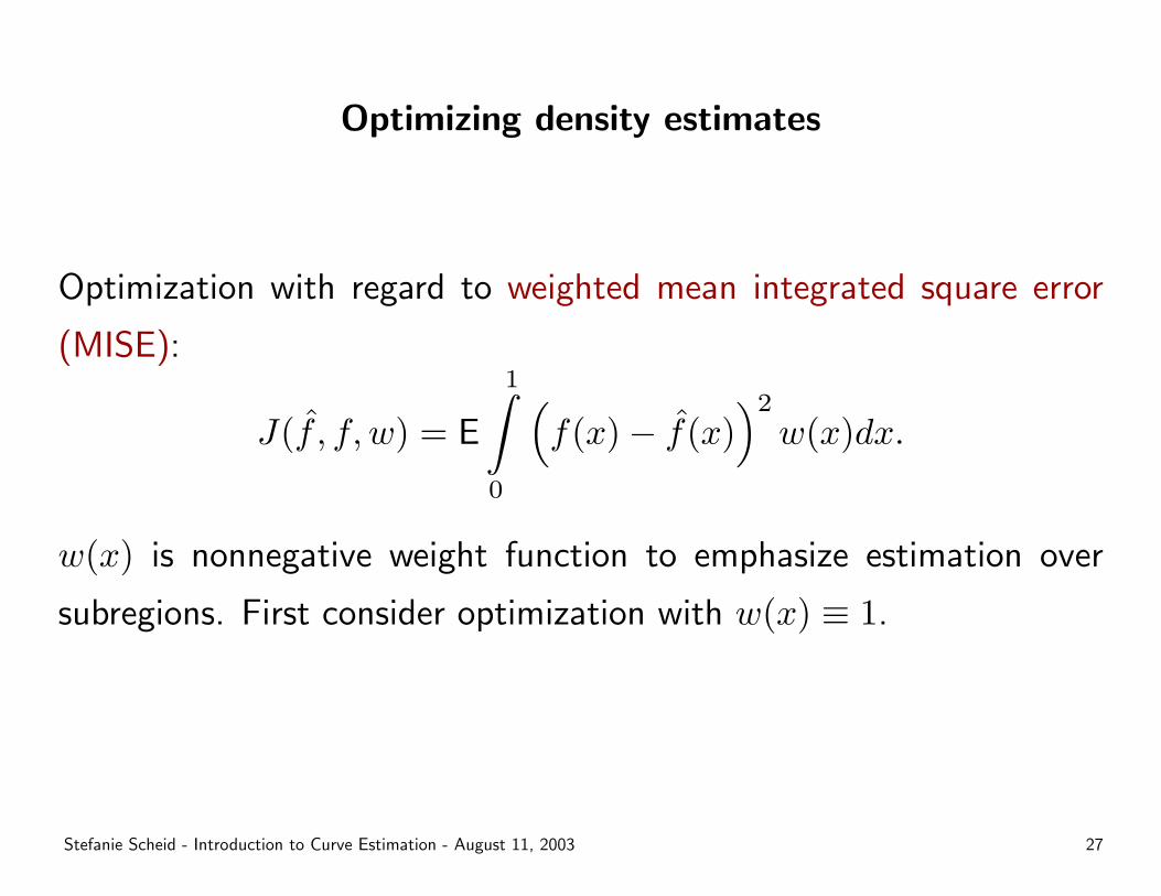
Optimizing density estimates
Optimization with regard to weighted mean integrated square error
(MISE):
J(f̂ , f, w) = E
1∫0
(f(x)− f̂(x)
)2
w(x)dx.
w(x) is nonnegative weight function to emphasize estimation over
subregions. First consider optimization with w(x) ≡ 1.
Stefanie Scheid - Introduction to Curve Estimation - August 11, 2003 27
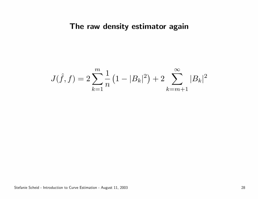
The raw density estimator again
J(f̂ , f) = 2m∑k=1
1n
(1− |Bk|2
)+ 2
∞∑k=m+1
|Bk|2
Stefanie Scheid - Introduction to Curve Estimation - August 11, 2003 28
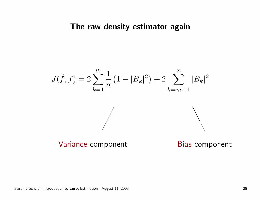
The raw density estimator again
J(f̂ , f) = 2m∑k=1
1n
(1− |Bk|2
)+ 2
∞∑k=m+1
|Bk|2
���������
Variance component
AAAAAAAAK
Bias component
Stefanie Scheid - Introduction to Curve Estimation - August 11, 2003 28
Single term stopping rule
– Estimate ∆Js = J(f̂s, f)−J(f̂s−1, f), gain of including sth Fourier
coefficient. MISE is decreased if ∆Js is negative.
– Include terms only if their inclusion results in negative difference.
Multiple testing problem!
– Inclusion of higher-order terms results in rough estimate.
– Suggestions: Stop after t successive nonnegative inclusions. Choice
of t is data/curve dependent.
Stefanie Scheid - Introduction to Curve Estimation - August 11, 2003 29
Other stopping rules
– Different considerations about estimating MISE lead to various
optimization concepts.
– Not at all generally superior to single term rule. Depends on curve
features.
Stefanie Scheid - Introduction to Curve Estimation - August 11, 2003 30
Multiplier sequences
– So far: “raw” estimate with bk = 1 or bk = 0.
– Now allow {bk} to be sequence tending to zero with increasing k.
– Concepts depend again on considerations about MISE.
– Question of advisable stopping rule remains.
Stefanie Scheid - Introduction to Curve Estimation - August 11, 2003 31
Two-step strategy with multiplier sequence
1. Estimate with raw estimator and one of former stopping rules.
2. Applying a multiplier sequence to the remaining terms will always
improve the estimate.
Stefanie Scheid - Introduction to Curve Estimation - August 11, 2003 32
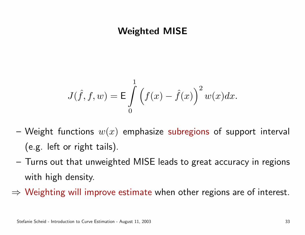
Weighted MISE
J(f̂ , f, w) = E
1∫0
(f(x)− f̂(x)
)2
w(x)dx.
– Weight functions w(x) emphasize subregions of support interval
(e.g. left or right tails).
– Turns out that unweighted MISE leads to great accuracy in regions
with high density.
⇒ Weighting will improve estimate when other regions are of interest.
Stefanie Scheid - Introduction to Curve Estimation - August 11, 2003 33
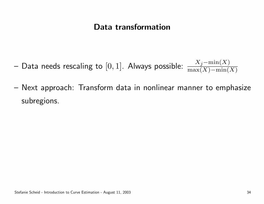
Data transformation
– Data needs rescaling to [0, 1]. Always possible:Xj−min(X)
max(X)−min(X)
– Next approach: Transform data in nonlinear manner to emphasize
subregions.
Stefanie Scheid - Introduction to Curve Estimation - August 11, 2003 34
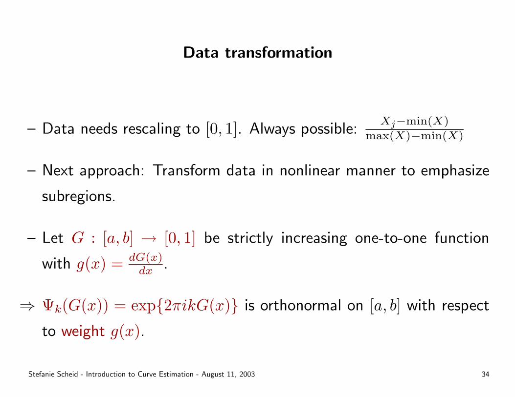
Data transformation
– Data needs rescaling to [0, 1]. Always possible:Xj−min(X)
max(X)−min(X)
– Next approach: Transform data in nonlinear manner to emphasize
subregions.
– Let G : [a, b] → [0, 1] be strictly increasing one-to-one function
with g(x) = dG(x)dx .
⇒ Ψk(G(x)) = exp{2πikG(x)} is orthonormal on [a, b] with respect
to weight g(x).
Stefanie Scheid - Introduction to Curve Estimation - August 11, 2003 34
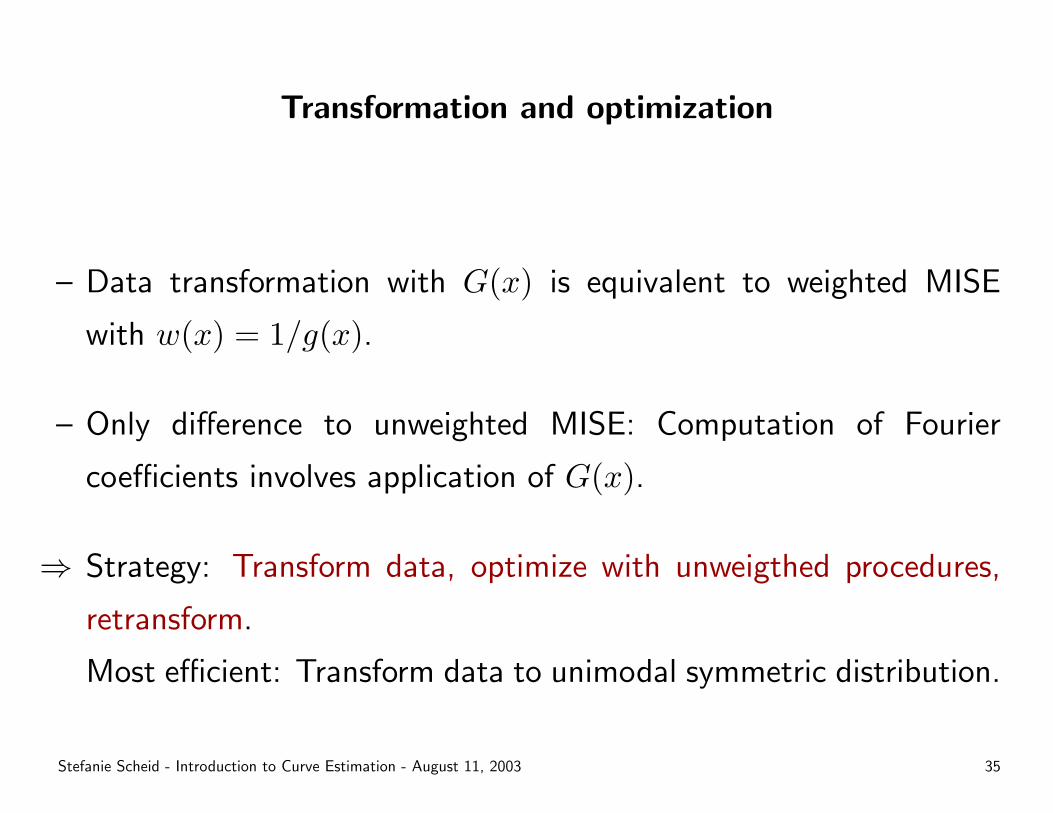
Transformation and optimization
– Data transformation with G(x) is equivalent to weighted MISE
with w(x) = 1/g(x).
– Only difference to unweighted MISE: Computation of Fourier
coefficients involves application of G(x).
⇒ Strategy: Transform data, optimize with unweigthed procedures,
retransform.
Most efficient: Transform data to unimodal symmetric distribution.
Stefanie Scheid - Introduction to Curve Estimation - August 11, 2003 35
Application to gene expression data
– Problem: Fitting two distributions to another by removing a
minimal number of data points.
– Idea: Estimate the two densities in an optimal manner. Remove
points until goodness-of-fit is high with regard to modified MISE.
Stefanie Scheid - Introduction to Curve Estimation - August 11, 2003 36