Introduction to Credit Scoring · the principle of “the investor's right to know.” In 1860...

An Introduction to Credit Scoring

For

Small and Medium Size Enterprises.

Javier Márquez.1

February 2008

I. INTRODUCTION.

This paper is intended as a quick primer on credit scoring, and how it applies to the assessment of risk of small and medium size enterprises (SME’s). It is part of a larger study on how credit scoring is currently being applied for this purpose, and exploring the possibility of broadening the applicability of the technique to encompass a wider spectrum of SME’s. Thus, the aim has been to provide the reader who wishes to understand what credit scoring is about but doesn’t want to become a specialist, with enough information on credit scoring fundamentals so as to feel comfortable with the subject in terms of its mechanics, scientific foundations, applicability and the practical issues that must be addressed for a successful application. It was deemed important to specifically compare credit scoring with ratings, since they are often confused and erroneously addressed as if they were the same or at least “close relatives”. Essentially, the only thing they have in common, is that both are systematic approaches to appraise the risk of an individual debtor; methodologically however, they are extreme opposites.

Ratings live in the realm of big companies that issue or contract large

debt, and the evaluation of the risk of the debtor is done employing the traditional techniques of fundamental analysis and experience. In contrast, credit scoring is based on discriminant analysis; a statistical methodology designed to “optimally” classify a population (e.g. debtors) into clearly distinguishable groups (e.g. “good” and “bad”). As such, it requires large populations so that the statistical parameters estimated are reliable, and provide a reasonable degree of certainty as to what group a particular member of the population belongs. Thus, for single obligor risk measurement, 1 The author wishes to thank Mr. Alberto Jones of Moodys’, Victor Manuel Herrera of Standard

and Poors, and Guillermo Mass and Juan Ramon Bernal of Banco Santander-Serfín for their

generous contributions to this effort. I would particularly like to thank Augusto de la Torre who,

in spite of my reluctance, encouraged me to undertake this project.

1

the technique only makes sense for large populations of debtors with fairly homogenous characteristics. Finally, whereas a rating is an ordinal risk indicator in the sense that higher ratings mean less risk and lower ratings imply more risk in the “opinion” of whoever did the rating, credit scores are actual estimates of default probabilities of debtors in a group, and their reliability depends on the sample in terms of size, the proportions of good and bad debtors it contains, and the mathematical model used to distinguish between them.

Ratings however, are by far the most common reference on individual

credit risk in the industry, for practical and regulatory reasons. Thus, no matter how individual credit risk is assessed, or how precise the technique used to estimate a default probability, it will eventually have to be related to a rating; either as a means to communicate in terms that are readily understood across all levels of a lender organization and regulators, as a means to comply with regulation, or both.

Section two gives a brief history of ratings and credit scoring. Besides

explaining how each technique caters to different types of debtor populations, it is interesting to see that, contrary to popular belief, credit scoring is not a recent fad, but dates back to over sixty years when consumer lenders were overwhelmed in their capacity to process personal loan applications, and something had to be done. In section three, the “anatomy” of credit scoring is explained: building “scorecards”, sample design, discriminant analysis and the issues that must be addressed in practice for successful applications. In the next section, we come full circle and show how, despite their differences, scores can be “mapped” into ratings, establishing an indispensable link between the two which, as already mentioned, is important both for practical and regulatory purposes. In this section, we also go into some detail on how it can be applied in the Basel II framework. The paper concludes with a discussion of the status of credit scoring as it applies to SME lending. It is seen why the tool is very useful at the low end of the scale, and substantiate the claim that in this population the use of credit scoring is widespread. However, it is also explained why the technique becomes less and less applicable as one moves up the ladder, until it becomes difficult or impossible to apply for the larger SME’s.

II. A BRIEF HISTORY OF THE SYSTEMATIC ASSESSMENT OF CREDIT RISK:

CREDIT RATINGS VS. CREDIT SCORING.

The essence of lending money has been understood from the very beginning and it is unlikely to change; namely, one needs to establish potential

2

debtors capacity and willingness to pay. Traditionally, since there is a recorded history of credit over 4000 years ago2 and of banking from the middle ages up to the beginning of the twentieth century, the assessment by bankers of the risk represented by potential debtors, in terms of their capacity and willingness to pay had hardly changed. There was a certain mystique surrounding the shrewd and exquisite banker with an infallible judgment who could, at a glance, determine the “quality” of a would be client. Thus, any banker worth his salt was supposed to have a profound knowledge of his clients and competition, which allowed him to decide by trade, pure instinct and trusting in a bit of luck3, who he could lend money to, how much he could lend them, how much he could charge, how he would be paid, and what collateral he could demand. Over the last half of the last century to the present day, this perception of banking has practically disappeared and over the past twenty five years, there has been a radical change in the way risk in general and credit risk in particular, is perceived, measured and managed.

Basically, the change is a direct response to the dramatic increase in complexity of the credit business, technology and financial knowledge. Whereas well into the nineteenth century bankers generally dealt with a relatively small client base (by today’s standards), of elite customers who could be “dissected” and evaluated on an individual basis, and a manageable number of relatively large loans could be tailored to individual needs, by the first quarter of the twentieth century, the potential client base had expanded enormously.

Although it is not the main subject of this paper, it is important to talk about ratings since they are often confused with scores. As shall be seen later, this does not mean however, that a relationship between ratings and credit scores cannot be established. In fact, a correspondence can be established and it has become a necessity for regulatory purposes, particularly in the light of the new Basel II accord, where capital charges due to risky assets can be either ratings dependent in the “standardized approach” or PD driven, in the Internal Ratings Based (IRB)” approach.

2.1. Ratings.

Large corporations, besides having access to banks, have been able to place debt in public offerings in the market for centuries. As the number of

2 Lewis reported in 1992, that a Babylonian stone tablet reads the inscription: “Two shekels of silver

have been borrowed by Mas-Schamach, the son of Adradimeni, from the sun priestess Amat-

Schamach, the daughter of Warad Enlil. He will pay the sun goddess interest. At the time of the

harvest he will pay back the sum and the interest upon it. 3 No traditional banker will admit gracefully to this “luck” component!

3

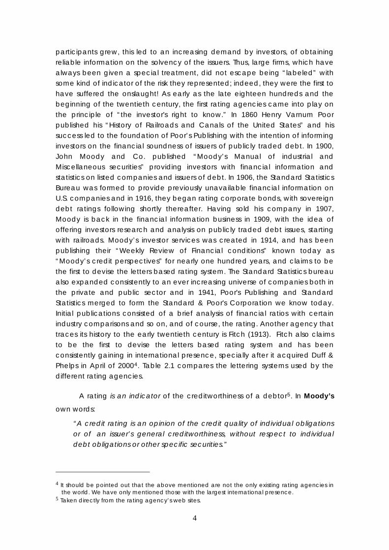
participants grew, this led to an increasing demand by investors, of obtaining reliable information on the solvency of the issuers. Thus, large firms, which have always been given a special treatment, did not escape being “labeled” with some kind of indicator of the risk they represented; indeed, they were the first to have suffered the onslaught! As early as the late eighteen hundreds and the beginning of the twentieth century, the first rating agencies came into play on the principle of “the investor's right to know.” In 1860 Henry Varnum Poor published his “History of Railroads and Canals of the United States” and his success led to the foundation of Poor’s Publishing with the intention of informing investors on the financial soundness of issuers of publicly traded debt. In 1900, John Moody and Co. published “Moody’s Manual of industrial and Miscellaneous securities” providing investors with financial information and statistics on listed companies and issuers of debt. In 1906, the Standard Statistics Bureau was formed to provide previously unavailable financial information on U.S. companies and in 1916, they began rating corporate bonds, with sovereign debt ratings following shortly thereafter. Having sold his company in 1907, Moody is back in the financial information business in 1909, with the idea of offering investors research and analysis on publicly traded debt issues, starting with railroads. Moody’s investor services was created in 1914, and has been publishing their “Weekly Review of Financial conditions” known today as “Moody’s credit perspectives” for nearly one hundred years, and claims to be the first to devise the letters based rating system. The Standard Statistics bureau also expanded consistently to an ever increasing universe of companies both in the private and public sector and in 1941, Poor's Publishing and Standard Statistics merged to form the Standard & Poor's Corporation we know today. Initial publications consisted of a brief analysis of financial ratios with certain industry comparisons and so on, and of course, the rating. Another agency that traces its history to the early twentieth century is Fitch (1913). Fitch also claims to be the first to devise the letters based rating system and has been consistently gaining in international presence, specially after it acquired Duff & Phelps in April of 20004. Table 2.1 compares the lettering systems used by the different rating agencies.

A rating is an indicator of the creditworthiness of a debtor5. In Moody’s

own words:

“A credit rating is an opinion of the credit quality of individual obligations or of an issuer’s general creditworthiness, without respect to individual debt obligations or other specific securities.”

4 It should be pointed out that the above mentioned are not the only existing rating agencies in

the world. We have only mentioned those with the largest international presence. 5 Taken directly from the rating agency’s web sites.

4

Speculative Grade

Invest-mentGrade

Associated Risk

Low

High

CCCCaCCCC

CaaCCCCCCBBBBaBBBB

BaaBBBBBBAAA

AaAAAAAaaAAAAAA

Moody’sS&PFitch

MoreMoreRiskRisk

Less Less RiskRisk

Table 2.1: Comparison of Rating Categories by Rating Agency.

Other rating agencies have similar definitions:

Standard & Poors:

“A credit rating is Standard & Poor’s opinion of the general creditworthiness of an obligor, or the creditworthiness of an obligor with respect to a particular debt security or other financial obligation, based on relevant risk factors. A rating does not constitute a recommendation to purchase, sell, or hold a particular security. In addition, a rating does not comment on the suitability of an investment for a particular investor”.

Fitch:

“Fitch's credit ratings provide an opinion on the relative ability of an entity to meet financial commitments, such as interest, preferred dividends, repayment of principal, insurance claims or counterparty obligations. Credit ratings are used by investors as indications of the likelihood of receiving their money back in accordance with the terms on which they invested”.

Evidently, credit rating has come a long way since the first agencies appeared a hundred years ago. Not only have they expanded their operations to cover the vast spectrum of firms and government agencies that publicly issue debt, but they have consistently refined and systematized their methods. There has also been a parallel development by banks, which employ very similar methods to evaluate the risk of their larger loans. In essence, and with the peculiarities pertaining to each agency or bank, the risk assessment or rating of a particular debt issue of a large debtor, is arrived at after a thorough fundamental analysis of the issuer and his obligations in relation to the particular issue. The quantitative analysis derived from historical data and future projections of financial statements under different business, market and

5

economic scenarios, is contrasted with qualitative appreciations of particular characteristics of the issuer, and the environment. Thus, things like the quality of management and the business strategy of the issuer, along with the competition and the regulatory requirements it faces, whose contribution to risk are not easily quantifiable, are carefully weighed before a recommendation or rating is proposed by the research team responsible for the analysis. The final recommendation or rating is assigned, only after the findings, both quantitative and qualitative, and the proposal of the research team have been discussed in a top level committee. Schematically, the process is presented in figure 2.1. below. It is interesting to see all the things that are considered, and the hierarchy assigned to each, in order to arrive at a rating and that qualitative analysis is placed at the very top of the pyramid.

QUALITATIVEQUALITATIVEANALYSISANALYSIS

ManagementManagementStrategicStrategic ManagementManagement

FinancialFinancial FlexibilityFlexibility

QUANTITATIVE ANALYSISQUANTITATIVE ANALYSIS

Financial StatementsFinancial StatementsPrevious OutstandingPrevious Outstanding

ProjectionsProjections

MARKET POSITIONSMARKET POSITIONS

SECTOR COMPETITIVE ENVIRONMENTSECTOR COMPETITIVE ENVIRONMENT

Global / DomesticGlobal / Domestic

REGULATORY ENVIRONMENT REGULATORY ENVIRONMENT

SECTORIAL ANALYSIS (INDUSTRY) SECTORIAL ANALYSIS (INDUSTRY)

MACROECONOMIC AND SOVEREIGN ANALYSISMACROECONOMIC AND SOVEREIGN ANALYSIS


QUALITATIVEQUALITATIVEANALYSISANALYSIS

ManagementManagementStrategicStrategic ManagementManagement

FinancialFinancial FlexibilityFlexibility

QUANTITATIVE ANALYSISQUANTITATIVE ANALYSIS

Financial StatementsFinancial StatementsPrevious OutstandingPrevious Outstanding

ProjectionsProjections

MARKET POSITIONSMARKET POSITIONS

SECTOR COMPETITIVE ENVIRONMENTSECTOR COMPETITIVE ENVIRONMENT


REGULATORY ENVIRONMENT REGULATORY ENVIRONMENT

SECTORIAL ANALYSIS (INDUSTRY) SECTORIAL ANALYSIS (INDUSTRY)

MACROECONOMIC AND SOVEREIGN ANALYSISMACROECONOMIC AND SOVEREIGN ANALYSIS


Figure 2.1. Standard Considerations in the rating process.

(Courtesy of Moody’s Investor Services.)

Although the general principles of fundamental analysis, as regards the evaluation of the credit worthiness of a debtor are well established, the actual methodologies of the rating agencies, and the internal rating systems used by banks are not publicly disclosed. In all cases they are considered an important part of the intellectual property of the banks and the agencies and key factors of their competitiveness in the industry. Indeed, both the rating agencies and the banks go to great lengths in trying to convince the market and the financial authorities that they do it as well as, or better than the rest. There is an important difference between the banks and the rating agencies however; namely, whereas banks are under no obligation to disclose their internal ratings to any one other than the financial authorities, disclosure of ratings is at the very heart of the rating agencies business. This permits the market and any interested observer to see what the actual track record of the agencies is, and how well the ratings actually capture the risk in rated debt issues.

6

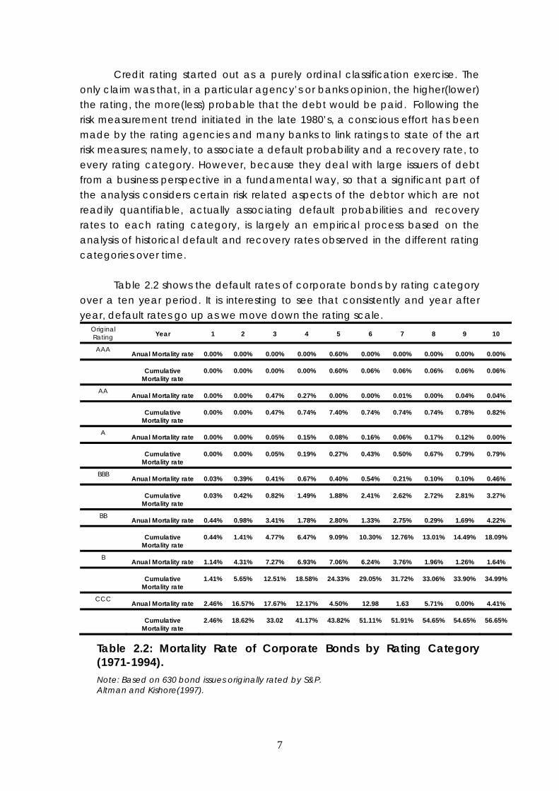
Credit rating started out as a purely ordinal classification exercise. The only claim was that, in a particular agency’s or banks opinion, the higher(lower) the rating, the more(less) probable that the debt would be paid. Following the risk measurement trend initiated in the late 1980’s, a conscious effort has been made by the rating agencies and many banks to link ratings to state of the art risk measures; namely, to associate a default probability and a recovery rate, to every rating category. However, because they deal with large issuers of debt from a business perspective in a fundamental way, so that a significant part of the analysis considers certain risk related aspects of the debtor which are not readily quantifiable, actually associating default probabilities and recovery rates to each rating category, is largely an empirical process based on the analysis of historical default and recovery rates observed in the different rating categories over time.

Table 2.2 shows the default rates of corporate bonds by rating category

over a ten year period. It is interesting to see that consistently and year after year, default rates go up as we move down the rating scale.

Original Rating Year 1 2 3 4 5 6 7 8 9 10

AAA Anual Mortality rate 0.00% 0.00% 0.00% 0.00% 0.60% 0.00% 0.00% 0.00% 0.00% 0.00%

Cumulative

Mortality rate 0.00% 0.00% 0.00% 0.00% 0.60% 0.06% 0.06% 0.06% 0.06% 0.06%

AA Anual Mortality rate 0.00% 0.00% 0.47% 0.27% 0.00% 0.00% 0.01% 0.00% 0.04% 0.04%

Cumulative

Mortality rate 0.00% 0.00% 0.47% 0.74% 7.40% 0.74% 0.74% 0.74% 0.78% 0.82%

A Anual Mortality rate 0.00% 0.00% 0.05% 0.15% 0.08% 0.16% 0.06% 0.17% 0.12% 0.00%

Cumulative

Mortality rate 0.00% 0.00% 0.05% 0.19% 0.27% 0.43% 0.50% 0.67% 0.79% 0.79%

BBB Anual Mortality rate 0.03% 0.39% 0.41% 0.67% 0.40% 0.54% 0.21% 0.10% 0.10% 0.46%

Cumulative

Mortality rate 0.03% 0.42% 0.82% 1.49% 1.88% 2.41% 2.62% 2.72% 2.81% 3.27%

BB Anual Mortality rate 0.44% 0.98% 3.41% 1.78% 2.80% 1.33% 2.75% 0.29% 1.69% 4.22%

Cumulative

Mortality rate 0.44% 1.41% 4.77% 6.47% 9.09% 10.30% 12.76% 13.01% 14.49% 18.09%

B Anual Mortality rate 1.14% 4.31% 7.27% 6.93% 7.06% 6.24% 3.76% 1.96% 1.26% 1.64%

Cumulative

Mortality rate 1.41% 5.65% 12.51% 18.58% 24.33% 29.05% 31.72% 33.06% 33.90% 34.99%

CCC Anual Mortality rate 2.46% 16.57% 17.67% 12.17% 4.50% 12.98 1.63 5.71% 0.00% 4.41%

Cumulative

Mortality rate 2.46% 18.62% 33.02 41.17% 43.82% 51.11% 51.91% 54.65% 54.65% 56.65%

Table 2.2: Mortality Rate of Corporate Bonds by Rating Category (1971-1994). Note: Based on 630 bond issues originally rated by S&P. Altman and Kishore(1997).

7

Data such as that of table 1.1 can be used to estimate default probabilities by rating category. Figure 2.2 shows Moody’s default probability estimates by rating category over time. It is interesting to see that default probabilities increase as ratings go down the scale, which is consistent with the behavior observed in the mortality rate data shown above6.

Figure 2.2: Default Probability by Rating Category

(Courtesy of Moody’s Investor Services.)

More recently, and specially after the Basel II initiative, banks who haven’t already done so, are strongly urged to work towards using rating systems which, to each rating category, can explicitly associate a default probability such as shown above, and an expected recovery rate in case of default. An example of recovery rates is presented in table 2.3 below.

Seniority No. of Bonds Recovery Rate (Mean)

Standard Deviation

Senior guaranteed 89 57.94% 23.12% Senior non guaranteed 225 47.70% 26.60% Senior subordinated 186 35.09% 25.28% Subordinated 218 31.58% 22.50% Junior subordinated 34 20.81% 17.76%

Table 2.3: Recovery Rates on Corporate Bonds by Seniority.

(% of face value of $100). Altman and Kishore(1997).

As seen above, the scrupulous recording of performance data by the agencies, has permitted the estimation of a wide variety of risk related measures. Simply to conclude this section with another recommendation of the Basel Committee, table 2.4 below shows a “transition matrix”, which provides 6 Although the numbers don’t necessarily coincide due to differences in rating scales and methodologies of the different rating agencies.

8

the probability of migration of rated bonds from one rating category to another.

Finally, it should be fairly obvious that rating a large corporate loan by a bank o

Rating AAA AA A BBB BB B CCC Default

r an agency, is a lengthy, labor intensive and costly affair, which is only justified by the magnitude of the debt relative to the analytical effort (cost) involved, and the broad interest manifest by the investor community. As one goes down the scale, doing such an in depth analysis becomes ever more costly, to the point of becoming prohibitive, and some would argue unnecessary. This does not mean that rating other types of loans is not done; quite the contrary. Over the years, rating systems for all sorts of loans(businesses,

AAA 94.30% 5.50% 0.10% 0.00% 0.00% 0.00% 0.00% 0.00%

AA 0.70% 92.60% 6.40% 0.20% 0.10% 0.10% 0.00% 0.00%

A 0.00% 2.60% 92.10% 4.70% 0.30% 0.20% 0.00% 0.00%

BBB 0.00% 0.00% 5.50% 90.00% 2.80% 1.00% 0.10% 0.30%

BB 0.00% 0.00% 0.00% 6.80% 86.10% 6.30% 0.90% 0.00%

B 0.00% 0.00% 0.20% 1.60% 1.70% 93.70% 1.70% 1.10%

CCC 0.00% 0.00% 0.00% 0.00% 9.00% 2.80% 92.50% 4.60%

Table 2.4: Transition Matrix.

Source: Altman and Kao (1992), estimated from data on bonds issued between 1971 and 1989,

consumer or personal loans) have been devised, where loan applicants

.2. Credit Scoring.

With the growth of the middle class in the eighteen hundreds, money lender

rated by S&P.

provide information through a questionnaire of some sort, which is then processed by a credit analyst, who rates and decides to grant or reject the loan, based on experience and intuition. Initially the information required was purely judgmental, and depended heavily on analysts personal opinions of what determined capacity and willingness to pay. It quickly became evident that in many cases, there were rating inconsistencies due to differences of opinion between analysts. Furthermore, the number of applications kept growing, to the point that analysts were overwhelmed, and something else was needed. This brings us to the main subject.

2

s realized there was a rapidly growing market in smaller loans with the added attraction of diversification and the ensuing protection in large

9

numbers. This gives rise to the creation of the first commercial banks, pawn brokers and even mail order services7; all catering to consumer credit. The process really takes off in the 1920’s with the possibility of the public at large to buy automobiles. This however required a radical change in the way of doing business; namely, there was a need to standardize products and systematize the loan origination and management process. In today’s environment, this has become an imperative. Since the typical debtor is lost in the anonymity of the great mass of individuals that owe banks or other consumer creditors money, it is prohibitive to carry out an evaluation of the risk they represent based solely on secrets of the trade, intuition, pure experience or even a rating process as previously described; some kind of automatic classification of the “quality” of debtors has become a necessity.

Credit scoring is the first formal approach to the problem of assessing the credit

Shortly after the war, with the advent of automatic calculators that eventu

risk of a single debtor in a scientific and automated way, in direct response to the need of processing large volumes of applications for relatively small loans. During the nineteen thirties some mail order companies already overwhelmed with demand, devised scoring systems in an attempt to overcome the inconsistencies detected in the credit granting decisions of different analysts. Thus, observable attributes of good or bad debtors were identified, measured and numerically graded accordingly, to produce a final score as a simple sum of the individual components. In many cases the score was associated with a rating. When credit analytical talent and expertise became scarce during WWII, companies engaged in consumer credit on a large scale, asked experienced analysts to write down the rules which led them to decide whether or not they would give someone credit. The result was a hybrid assortment of different kinds of scoring systems and a variety of conditions which experience had taught should be met, if a loan was to have a reasonable chance of performing8.

ally led to full fledged computers, the processes described became subject to automation. The scientific background to modern credit scoring is provided by the pioneering work of R. A. Fisher(1936) who devised a statistical technique called discriminant analysis, to differentiate groups in a population through measurable attributes, when the common characteristics of the

7 Mail order services began as clubs in Yorkshire in the 1800’s, and were restricted to small segments of

the population for very special purposes. 8 Note that this is very similar to an expert system.

10

members of the group are unobservable9. In 1941 D. Durand recognized that the same approach could be used to distinguish between good and bad loans. Mating automation with statistical discriminant analysis was a natural route for credit scoring to follow, eliminating the largely subjective rules of thumb adhered to by analysts, regardless of their validity10. Obviously, the route to success was heavily mined, since establishing creditworthiness of a debtor using an automated process based on discriminant analysis was viewed as a frontal attack on conventional banking wisdom, painstakingly acquired through several millennia. The most famous anecdote is that of E. F. Wonderlic, president of Household Finance Corp. (HFC) in the early 1940’s. Wonderlic was well versed in statistics through his training in psychology, and tried to implement credit scoring in HFC. His frustration at the rejection of the technique is evident in his 1948 report where, after proving that credit scoring actually worked, in a way that any audience technically qualified in statistical techniques would have readily accepted, he pleaded: “These figures from actual results should prove conclusively to the most skeptical that the Credit Guide Score is a tool11 which is consistently able to point out the degree of risk in any personal loan, provided, of course, that it is correctly scored”. That his concern was well founded was corroborated when it was later discovered that many analysts approved loans first, and then filled in the “scorecard” to show a passing score.

Perseverance prevailed however, and more systems were developed. Initially, both the variables selected and the scores assigned were mainly judgmental, but the systematic application of the methods contributed with uniformity of scoring criteria providing the credit origination process with sorely needed consistency and predictability. The economics of processing the exponential growth in personal loan applications, along with increasingly refined statistical techniques with the ensuing improvement of the predictive power of the models, and the constant advances in available computing power, which inexorably reduced application processing time, ultimately forced the acceptance of statistically based, automated scoring systems. The introduction of credit cards in the 1960’s provided further impulse for the extensive use of credit scoring in banks, retailers, and any large consumer lender. Curiously, the issuance in the U. S. of the “Equal Credit Opportunity Acts”

9 Fisher was concerned with the problem of differentiating between two varieties of Iris by the size of the

plants and the origins of skulls by their physical measurements. 10 As previously mentioned, hybrid systems where scoring interacts with expert rules is the domain of

artificial intelligence. See for example Cuena, et. al. (1990). 11 “The Credit Guide Score” was the manual distributed through HFC indicating how credit applications

should be scored.

11

and its amendments in 1975-76 ensured the complete acceptance of credit scoring. It became illegal to reject a loan on the basis of gender, religion, or race, unless it “was empirically derived and statistically based”. Thus, the impartiality in the assessment of would be debtors is generally accepted as one of credit scoring’s main virtues, and leave it to statistics to decide whether a particular characteristic is riskier than another.

This has not gone uncontested however. In several countries different types of activists have lobbied intensively to forbid the use of variables relative to gender, race and creed arguing they could produce discriminatory results, despite evidence to the contrary. In 1976 for example, Chandler and Ewert showed that if gender were allowed to be a scoring variable, more women than men would have access to credit12. Many consumers also object to credit scoring, feeling demeaned by being treated impersonally as “just a number or another member of the group”, and helpless to plea their case when rejected. The issue is really one of “impersonal” versus “impartial” which gives rise to a lively, endless and largely unsettled discussion, since deciding which variables are “politically correct” and which are not, and if and when personal attention is warranted for some cases, pertains more to the realms of ethics or business practice and is therefore highly subjective13. The variables actually used in scorecards for consumer loans are no secret, and anybody who has filled in an application for a credit card, mortgage or car loan knows what they are: Besides name and address, the relevant variables refer to education, employment, how many years in the job, number of dependants, salary and other sources of income (investments etc.), properties and possessions (houses, cars etc.), other debts, bank and personal references and so on. This information is usually complemented with payment history data obtained from the public registries.

Today, it is literally prohibitive, both for considerations of financial risk assessment and in terms of required manpower, to engage in consumer lending activities in any other way. To the chagrin of die-hard traditional analysts, by 1963 default rates in consumer loans screened with credit scoring techniques, had dropped by 50% or more.14 This success invariably led money lenders to try credit scoring in other types of loans, e.g. personal, car or mortgage loans. A case which is of particular interest, is the parallel effort by E. Altman (1968) who first proposed a scoring technique to predict the risk of

12 Among other things, the main reason is that in low income groups with part time employment, women

are generally better than men at repaying their debts. 13 See for example Churchill and Nevin (1979), Capon (1982) and Saunders (1985) for arguments on both

sides of the table. 14 See Meyers and Forgy(1963) and Churchill et. al.(1977).

12

companies going bankrupt. The discussion of Altman’s z-score method will help to illustrate the concept, before going into credit scoring in a more rigorous way in the next section.

2.3. A classical example of Credit Scoring: Altman’s Z-Score.

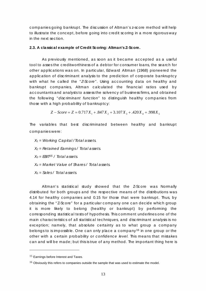
As previously mentioned, as soon as it became accepted as a useful tool to asses the creditworthiness of a debtor for consumer loans, the search for other applications was on. In particular, Edward Altman (1968) pioneered the application of discriminant analysis to the prediction of corporate bankruptcy with what he called the “Z-Score”. Using accounting data on healthy and bankrupt companies, Altman calculated the financial ratios used by accountants and analysts to assess the solvency of business firms, and obtained the following “discriminant function” to distinguish healthy companies from those with a high probability of bankruptcy:

54321 998.420.107.3847.717.0 XXXXXZScoreZ ++++==−

The variables that best discriminated between healthy and bankrupt

companies were:

X1 = Working Capital /Total assets.

X2 = Retained Earnings / Total assets.

X3 = EBITT

15 / Total assets.

X4 = Market Value of Shares / Total assets.

X5 = Sales / Total assets.

Altman’s statistical study showed that the Z-Score was Normally distributed for both groups and the respective means of the distributions was 4.14 for healthy companies and 0.15 for those that were bankrupt. Thus, by obtaining the “Z-Score” for a particular company one can decide which group it is more likely to belong (healthy or bankrupt) by performing the corresponding statistical tests of hypothesis. This comment underlines one of the main characteristics of all statistical techniques, and discriminant analysis is no exception; namely, that absolute certainty as to what group a company belongs to is impossible. One can only place a company16 in one group or the other with a certain probability or confidence level. This means that mistakes can and will be made; but this is true of any method. The important thing here is

15 Earnings before Interest and Taxes. 16 Obviously this refers to companies outside the sample that was used to estimate the model.

13

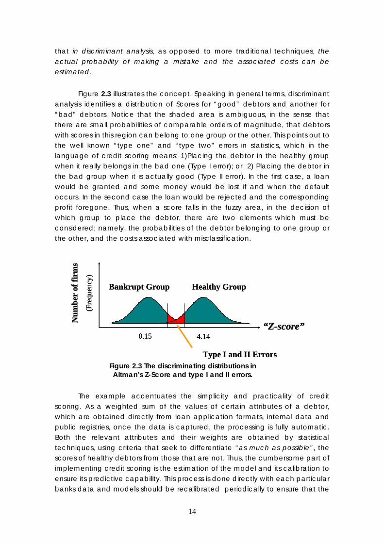
that in discriminant analysis, as opposed to more traditional techniques, the actual probability of making a mistake and the associated costs can be estimated.

Figure 2.3 illustrates the concept. Speaking in general terms, discriminant analysis identifies a distribution of Scores for “good” debtors and another for “bad” debtors. Notice that the shaded area is ambiguous, in the sense that there are small probabilities of comparable orders of magnitude, that debtors with scores in this region can belong to one group or the other. This points out to the well known “type one” and “type two” errors in statistics, which in the language of credit scoring means: 1)Placing the debtor in the healthy group when it really belongs in the bad one (Type I error); or 2) Placing the debtor in the bad group when it is actually good (Type II error). In the first case, a loan would be granted and some money would be lost if and when the default occurs. In the second case the loan would be rejected and the corresponding profit foregone. Thus, when a score falls in the fuzzy area, in the decision of which group to place the debtor, there are two elements which must be considered; namely, the probabilities of the debtor belonging to one group or the other, and the costs associated with misclassification.

BankruptBankrupt GroupGroup Healthy Group

““ZZ--scorescore””0.15 4.14

Type I and II Errors

Num

ber

Num

ber o

foffir

ms

firm

s

(( Fre

quen

cyFr

eque

ncy ))

BankruptBankrupt GroupGroup Healthy Group

““ZZ--scorescore””0.15 4.14

Type I and II Errors

Num

ber

Num

ber o

foffir

ms

firm

s

(( Fre

quen

cyFr

eque

ncy ))

Figure 2.3 The discriminating distributions in Altman’s Z-Score and type I and II errors.

The example accentuates the simplicity and practicality of credit scoring. As a weighted sum of the values of certain attributes of a debtor, which are obtained directly from loan application formats, internal data and public registries, once the data is captured, the processing is fully automatic. Both the relevant attributes and their weights are obtained by statistical techniques, using criteria that seek to differentiate “as much as possible”, the scores of healthy debtors from those that are not. Thus, the cumbersome part of implementing credit scoring is the estimation of the model and its calibration to ensure its predictive capability. This process is done directly with each particular banks data and models should be recalibrated periodically to ensure that the

14

model adapts to economic conditions and the dynamics of the market. All of this is explained in the next section, and the main techniques of discriminant analysis are presented in some detail in appendix “A”.

III. The Anatomy of Credit Scoring Techniques.

In this section we discuss the “what and how” of credit scoring. We begin by describing the “scorecard” , followed by a discussion of its principal elements and the relevant practical issues; namely, the applicants characteristics and attributes, accept/reject cut-offs, the definition of “good” and “bad” debtors, sample design and so on. The section ends with a brief description of “discriminant analysis”, which is the main statistical tool used for building scorecards17.

3.1. The Mechanics of Credit Scoring.

As illustrated by the previous example, credit scoring is an eminently pragmatic and empirical approach to the problem of risk assessment of individual debtors. The emphasis is on predicting defaults, not on explaining why they do or don’t occur. The basic elements of credit scoring are: 1) A set of categories of information called “Characteristics” or “Variables” with their corresponding “attributes”, which qualify and/or quantify how each characteristic applies to an individual debtor, 2) The points associated to a particular attribute as it pertains to an applicant and 3) A threshold or “cut-off value”.

In credit scoring terms, characteristics refer to the questions asked, whereas attributes are the specific answers to these questions, whether they be provided by the applicants or obtained from other sources, such as internal bank data or public registries. The words characteristic and variable are synonymous18, although the first is descriptive of the type of information comprised in each category, while the latter emphasizes the random nature of the information within a particular category. For example, a typical Characteristic or Variable considered in consumer loans is, “Residential Status”. Note however, that the actual number of attributes (possible “allowed” answers to a question) pertaining to this category can vary widely from one creditor to another. Whereas one might be happy with only two (dichotomous) attributes 17 A more detailed presentation will be found in Appendix A. 18 “Characteristic” would be the word used by the credit analyst using the model, whereas “variable” would be the word used by the statistician doing the estimation and calibration.

15

like owner-renting, another might require more specifics such as: owner with no mortgage, owner with a mortgage, rent unfurnished, rent furnished or living with parents. Assuming for the moment that attributes are scored with integers from naught to five, where higher is better, in the first case “owner” might merit a five while “renting” might merit a two. In the second case, five could be the score of “owner no-mortgage”, four for “owner with mortgage” and so on down the line to a zero for “living with parents”.

This little example illustrates the typical scoring structure used in practice; namely: Although, as was the case for Altman’s z-score, characteristics with single attributes scored with continuous values can be used, current practice favors a finite number of attributes (at least two) associated with each characteristic and in general, the points associated to each attribute are two digit numbers. Attributes associated to each characteristic are intended to be comprehensive and mutually exclusive; i.e. only one in each characteristic is pertinent to an applicant, and no question can go unanswered. In the name of practicality, parsimony is the name of the game; the less characteristics, attributes and scores you can get away with, without sacrificing the predictive capability of the model, the better. In principle, characteristics and attributes are determined solely on the basis of their predictive capacity. As such, save for legal restrictions such as those mentioned in the previous section, anything goes: regardless of whether or not a characteristic conforms to intuition or conventional wisdom, If it aids prediction it is included, and discarded otherwise.

In its simplest form, the typical scoring sequence of an application, is to “score” each characteristic with the points of the pertinent attribute, and add over all the characteristics to obtain a total score. Now the third element comes into play: The total score is compared to the threshold or cut-off value and, if it exceeds the threshold, the loan is granted; it is rejected otherwise.

3.2. The Scorecard.

The scorecard is the “organizer” of the mechanical procedure of credit scoring described in the preceding section, and is best explained with an example. Consider a simple scoring exercise in a small regional bank for a loan to a small local business, and assume that only six characteristics are required to asses the risk of applicants in this credit category; namely: The Age of the Applicant, Years of the Business, Liquidity Ratio, Debt to Net Worth, Previous Experience with the Bank, and Maximum Delinquency Ever from the Public Registry. Table 2.1 shows how characteristics, attributes and points are organized in the corresponding “Score Card”. Notice that characteristics 3 & 5 are directly related with the capacity to pay, 2 & 4 directly address the

16

willingness to pay, and the first two are behavioral and indirect indicators of capacity/willingness, as dictated by experience. The table shows the attributes that correspond to each characteristic and their associated points.

The scoring process is straight forward. For example, consider a 43 year

old entrepreneur who’s been in business for 8 years. His financials show a liquidity ratio of 62% and a Debt to Net worth of 37%. Finally, His previous experience with the bank shows no past due payments over 30 days and the information from the public registry confirms this, showing maximum delinquency ever to be thirty days. Referring to the scorecard presented in table 3.1, this applicants score is “12.5”:

SCORE = 2.0 + 1.5 + 1.0 + 3.5 + 2.0 + 2.5 = 12.5

Notice that in the last row of each panel is a line labeled “NEUTRAL”, which is the cut off reference for each characteristic; i.e. 1.5 for “Age of Applicant”, 1.0 for “Years of Business” and so on. The Neutral attribute serves several purposes; first and foremost, the sum of their points (1.5 + 1.0 + 2.0 + 1.0 + 2.0 + 3.0 = 10.5) is the overall accept/reject threshold. Since his score (12.5) exceeds the threshold (10.5), our 43 year old entrepreneur will be granted his loan. Notice that this is the case, despite the fact that his points in two of the characteristics were below the neutral value; namely (1.0 < 2.0) in “Liquidity Ratio” and (2.5 < 3.0) in “Maximum Delinquency Ever”. Thus, the second reason that the Neutral attribute is important is that it allows the analyst who oversees the automatic scoring process, to detect where the weaknesses of the applicant lie, and override the systems assessment (one way or the other) if warranted19. Obviously, this only happens when the score’s proximity to the threshold casts a doubt on the verdict from the mechanical procedure. Although in most instances of consumer lending the rule is applied blindly, in the case of SME’s, this grey area is in the order of ± 10% around the overall accept/reject threshold. In many cases, there are even automatic overrides programmed into the system; in other words, if a score falls in the grey area, another set of tests are performed automatically which either narrow down the grey area or ultimately decide the issue mechanically. In countries like the U.K.20 lenders are encouraged to give rejected applicants the right to appeal, anticipating mistakes such as typographical errors or incorrectly captured data. Furthermore, a rejected applicant may consider that there is relevant information outside that contemplated in the application form, and therefore merits a personal revision that can help his case and change the decision.

19 Normally, in the best case he would have to have authorization from his supervisor. If the

application is for a relatively large loan, he would have to go through a committee. 20 The U.K. Guide to Credit Scoring (2000).

17

Another important property of the Neutral attribute is that it honors its name; that is, scoring a characteristic with the Neutral attributes points, does not incline the balance one way or the other. This is because in this case, the points are picked so that they are “prediction neutral”; neither aiding or hurting the applicants cause, when a characteristic is scored so. This is useful when for some reason or other, the answer provided by the applicant is ambiguous. (e.g. marking more than one attribute etc.), the default choice is the Neutral attribute.

1. AGE OF APPLICANT (Owner) 2. YEARS OF THE BUSINESS

(Company) ATTRIBUTES POINTS ATTRIBUTES POINTS Less than 30 years 0.0 Less than 2 years 0.0 30 years – 34 years 0.5 2 years – 3 years 11 months 0.5 35 years – 39 years 1.5 4 years – 4 years 11 months 1.0 40 years – 49 years 2.0 5 years – 9 years 11 months 1.5 50 years – 59 years 2.5 10 years or more 2.5 60 years or more 2.0 No Answer 0.0 No Answer 0.0 NEUTRAL 1.0 NEUTRAL 1.5

3. LIQUIDITY RATIO (Company) 4. PREVIOUS EXPERIENCE WITH THE BANK

(Company) ATTRIBUTES POINTS ATTRIBUTES POINTS Less than .25 0.0 New client, Less than 6 months 1.0 .25 - .74 1.0 More than 30 past due 0.0 .75 - .99 1.5 No past due payments over 30 days 2.0 1.00 – 1.24 2.0 No past due payments 2.0 1.25 – 1.74 3.0 No enquiries 1.0 1.75 or more 3.5 NEUTRAL 1.0 Cannot be calculated 0.0 NEUTRAL 2.0

5. DEBT / NET WORTH (Company)

6. MAXIMUM DELINQUENCY EVER (Company and/or Owner)

(Public Registry) ATTRIBUTES POINTS ATTRIBUTES POINTS Less than .25 4.0 No investigation (Q) 3.0 .25 - .49 3.5 No record (R) 3.0 .50 - .74 3.0 No Trade Lines (N) 2.5 .75 - .99 2.5 No Usable Trade Line (I) 2.5 1.00 – 1.24 2.0 Charge Off 0.5 1.25 – 1.74 1.5 120 + Days Delinquent (1) 1.0 1.75 – 2.99 1.0 90 Days Delinquent (2) 1.5 3.00 or more 0.5 60 Days Delinquent (3) 2.0 Cannot be calculated 0.5 30 Days Delinquent (4) 2.5 NEUTRAL 2.0 Unknown Delinquency (5) 3.0 Current and Never Delinquent (7) 4.5 Too new to Rate(8) 3.0 All other (9) 3.0 NEUTRAL 3.0

18

Table 3.1: Simple Scorecard Example.21

21 This is a sample of six characteristics from an actual SME scorecard used in a Mexican Bank.

The points have been changed in compliance with the banks request.

19

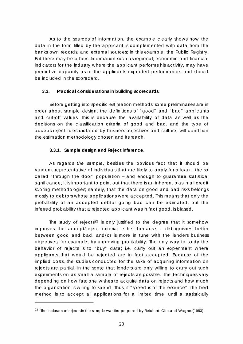
As to the sources of information, the example clearly shows how the

data in the form filled by the applicant is complemented with data from the banks own records, and external sources; in this example, the Public Registry. But there may be others. Information such as regional, economic and financial indicators for the industry where the applicant performs his activity, may have predictive capacity as to the applicants expected performance, and should be included in the scorecard.

3.3. Practical considerations in building scorecards.

Before getting into specific estimation methods, some preliminaries are in

order about sample design, the definitions of “good” and “bad” applicants and cut-off values. This is because the availability of data as well as the decisions on the classification criteria of good and bad, and the type of accept/reject rules dictated by business objectives and culture, will condition the estimation methodology chosen and its reach.

3.3.1. Sample design and Reject inference.

As regards the sample, besides the obvious fact that it should be random, representative of individuals that are likely to apply for a loan – the so called “through the door” population – and enough to guarantee statistical significance, it is important to point out that there is an inherent bias in all credit scoring methodologies; namely, that the data on good and bad risks belongs mostly to debtors whose applications were accepted. This means that only the probability of an accepted debtor going bad can be estimated, but the inferred probability that a rejected applicant was in fact good, is biased. The study of rejects22 is only justified to the degree that it somehow improves the accept/reject criteria; either because it distinguishes better between good and bad, and/or is more in tune with the lenders business objectives; for example, by improving profitability. The only way to study the behavior of rejects is to “buy” data; i.e. carry out an experiment where applicants that would be rejected are in fact accepted. Because of the implied costs, the studies conducted for the sake of acquiring information on rejects are partial, in the sense that lenders are only willing to carry out such experiments on as small a sample of rejects as possible. The techniques vary depending on how fast one wishes to acquire data on rejects and how much the organization is willing to spend. Thus, if “speed is of the essence”, the best method is to accept all applications for a limited time, until a statistically

22 The inclusion of rejects in the sample was first proposed by Reichert, Cho and Wagner(1983).

20

representative sample of rejects is obtained. If the decision is to reduce costs and spread them over time, what is generally done is to accept a random number of rejects (e.g. every tenth reject) until a good sample is obtained. This last scheme can be mixed with a scheme where all applicants with scores “not too far below” the rejection threshold (say 5 to 10%) are accepted, and below that, accept a random number.23 Apart from this, the determination of sample size, and the proportion of “goods” and “bads” that should be put in the sample, are estimated according to standard statistical techniques. It is also standard practice to set aside a “control sample” containing good and bad loans on which to back test the model. Although “the more the merrier”, one must strike a balance between available data, the size of the sample and it’s relevance in terms of how well the data represents the current market situation. This means that information should be as recent as possible -12 to 24 months old - and that there should be enough data to ensure statistical significance of the results. According to Lewis (1992) sample sizes of 3000 where the proportion of goods to bads is around 50-50 is a good place to start; Siddiqi (2006) says that a sample of 2000 each of goods and bads is adequate. If reject study is desired, then an additional 2000 rejects should be considered in the sample. An important practical consideration is that typically, the population is strongly one sided since the goods outnumber the bads in ratios of at least twenty to one, so that actually having samples with equal numbers of goods and bads, may be difficult to obtain. In this case put in all the bads you can get, and “enough” goods so as to minimize statistical error. Other issues on sample selection have to do with things like segmentation, augmentation, adjustments and so on. The need for segmentation arises from the fact that applicants in different regions, income categories or lines of business, may behave differently to the same characteristics and attributes, so that the weights which classify them into good or bad are different. Augmentation has to do with the feasibility and desirability of “augmenting” the sample as new data is received. Adjustment has to do with “over sampling” when there is apriori knowledge on the goods/bads ratio of the “through the door population”, and the differences with the available data24.

23 See for example Thomas et. al. Ch. 8. and Siddiqi Ch. 6. 24 There are many other technical considerations that must be addressed which cannot be

discussed here due to limitations of space. The reader who wishes to expand on the subject is encouraged to consult the specialized bibliography e.g. Thomas et. al. Ch. 8 and Siddiqi Ch. 6.

21

3.3.2. The definition of “bad”. Notice that the selection of the sample requires in all cases that the “good” debtors can be distinguished from the “bad” which must be defined25. Again, pragmatism, in the sense that the classification rule resulting from the definition is easy to interpret and the performance of the accounts can be tracked over time, is essential. The definition must also conform to product characteristics and business “culture” and objectives, so that definitions can vary widely from one creditor to another. For example, whereas a very common rule is to classify any debtor delinquent in three consecutive payments as bad, there are creditors that favor distinguishing between different levels of delinquency as they are related to pricing and profitability. For example, an account that is consistently thirty days overdue, but never rolls over to two or three, can be very profitable if properly priced. Other definitions can also take into account the dollar value of losses in case of delinquency. Notice that the definition adopted will have a direct impact on the sample selection and size, for the reasons previously explained. In general, the “tighter” the definition (e.g. “write-off” or “120 days delinquent”), the harder it will be to get the required number of bad accounts for the sample, whereas the opposite is true in “looser” definitions (e.g. “30 days in arrears”). This points out the trade off between the precision in the definition of bad, and the data count required for a good statistical fit, and leads to the next topic.

3.3.3. The cut-off value. Determining the accept/reject threshold is basically a balancing act between data availability which is a structural constraint, and the business priorities of the lender in terms of number of accounts that leads to the achievement of the objectives of the firm. Thus, if lowering the cut-off means increasing the number of accounts and more profits in spite of higher costs, and profits are the prime objective, it should be done. However, there are cases where profits don’t even enter the equation. For example, the objective may be to simply reduce losses to a certain proportion of asset value; or increase the approval rate to gain market share while maintaining costs at a certain level; define a cut-off that improves the overall turn around and reduce organizational costs or simply maximize the predictive power of the model. All of these criteria are currently used to determine the threshold.

25 By convention, “good” is everything that isn’t “bad”.

22

Cut-off parameters are obtained directly from the statistical estimation procedure used to fit the model to the sample data, and minimally, should correspond to expected accept and reject rates in line with company objectives. A rigorous analysis however, demands the examination of other metrics where the impact of the accept/reject rates are associated to the corresponding expected ratio of goods to bads of the accepted accounts, and the impact of the rule on profitability, revenues and costs, should be carefully assessed.

The simplest cut-off rule was illustrated in section 3.2, and it is called a

“hard low side cut-off” because it leaves no room for overriding the mechanical accept/reject decision. As mentioned in that section, because we are dealing with uncertainty, the most common rule is to define a gray area around the hard cut-off of ± 5 to 10% where applications whose scores lie in this interval, are referred to automatic override tests and/or manual scrutiny for the final decision. Some organizations use more complex cut-off rules, associating scores to different credit limits. For example, suppose that Tmin=T0,, T1, T2, ….Tn=Tmax are the finite number “n” of thresholds or cut-offs defined by a lender to determine credit limits “Li” depending on applicants scores. Then, the rule could go along the following lines26:

niTScoreifL

TTifLTif

LimitCredit iii ,...2,1;ScoreScore0

maxmax

1

min

=⎪⎩

⎪⎨

⎧

>≤<

<= −

Thus, the loan would be granted if it does not exceed the limit that corresponds to the applicants score. If the loan exceeds the limit, the lender can propose a smaller loan, refer to manual scrutiny to see if an override is in order and so on. The rule can be easily modified to give it continuity: assume that “Li” is the adequate level of credit corresponding to a score equal to cut-off value “Ti”, and let

iiii

ii TScoreTif

TTTScore

≤<−−

= −−

−1

1

1λ The following rule provides a continuous credit limit according to the score:

26 This rule and the next are only meant to illustrate the possibilities and the author makes no

claim as to their desirability for practical use.

23

( )⎪⎩

⎪⎨

⎧

>≤<−+

<= −−

maxmax

11

min

Score1Score0

TScoreifLTTifLL

TifLimitCredit iiiiii λλ

This highlights the fact that, given the lenders data constraints, business culture and objectives, the type of rule chosen is limited only to the imagination and technical capabilities of the analyst.

3.3.4. Other complementary tools: Behavior Scoring. Besides the preceding, there are other practical issues which should be

addressed when implementing credit scoring in an organization. For example, the effort and focus are not the same if there is previous experience and one is engaged in a reengineering, updating or refinement process, as those of setting up a system from scratch. A topic that must be addressed, is that of “behavioral scoring”. It should be evident that setting up a credit scoring system, implies a substantial investment in infrastructure; namely computers, software and qualified people. Furthermore the use of the scoring system necessarily entails the systematic accumulation of data of ever increasing quality on current clients and applicants. Thus, the same resources and data can be used for other purposes, besides credit origination; in particular, the monitoring of existing accounts, to determine how the risk profile of current debtors evolves over time. This allows the organization to anticipate cash flows and potential problems, adjust credit limits and interest rate spreads depending on the behavior of different clients and so on, in a dynamic way.

The use of the same credit scoring techniques and tools can be used for

predicting the behavior of existing accounts – hence the term – with the important difference of having better information, then at the time of acceptance. Thus, behavior scoring is aimed at determining the probability of clients remaining in or returning to a satisfactory status, and allows the organization to differentiate between clients. The differentiation should contemplate assessments on changes in the debtors characteristics such as, past and current delinquency levels, time on books, amounts delinquent, whether the account exceeds the limit and by how much, among others. Some users even make assessments on the probability of continued delinquency for currently delinquent clients. Typically, the types of additional useful statistics on clients, are of a historical nature. For example, it is possible to associate scores with the odds of an account performing well. The topic is too vast to dwell on,

24

but the reader is strongly advised to do some further reading27. Suffice it to say that in this day and age, every serious user of credit scoring is also a user of behavior scoring.

3.4. The Scientific Ingredient: Statistical Methods for Building Scorecards.

From the initial development of Credit Scoring Models (CSM´s) in the 1950’s and 1960’s to the present day, the most popular methods used to build credit scorecards are statistical discrimination and classification methods. The main reason is that they’ve been around a long time, so that they are well understood, and bring with them a wide assortment of useful analytical tools: from the properties of sample estimators to hypothesis testing and confidence intervals. In the credit scoring context, these tools permit the measurement of the relative predictive or discriminatory capacity of different characteristics and their attributes, as well as the estimation of the “best”28 choice of “points” or weights to associate to the attributes. This in turn allows the models to be “calibrated” or “fine tuned”, by retaining characteristics with good predictive power and discarding those which add little or nothing to the discriminatory capacity of the model, in the endless quest to keep things as simple as possible. They also provide enormous flexibility for the adaptation of the models to the ever changing circumstances, where the relative importance of characteristics may change. Some may even become irrelevant and must be discarded altogether, to be replaced by new ones with more predictive power.29

Although many proposals exist, in what follows, only the most widely used

statistical techniques are discussed. At the end of this section other approaches that have been proposed will be mentioned, and the interested reader will find technical literature on the subject in the bibliography. The following standard notation will be used:

X = {X1, X2, …,Xm} denotes the set of characteristics or random variables

that have predictive power of applicants performance (good/bad), and are directly associated to available information (i.e. from the application form, public registries, internal records etc.) on applicants. The vectors “xi” denote the attributes associated to Variable “Xi”, so that the components “xij” of an

27 See for example Hopper and Lewis 2002. 28 It is important to point out that there are different criteria of what is “best”, or in what sense

certain choices of weights(points) are better than others. Thus, the choice of optimizing criteria is a matter of taste, highly subjective and subject to debate.

29 For example, initially, having a bank account was a relatively important characteristic, which has virtually lost predictive power in developed markets as this is today common practice with debtors. A more relevant characteristic along these lines is whether or not the applicant has an account with the lender bank.

25

attribute vector are the values that the corresponding random variable can take; that is, the possible answers to the particular question which “Xi” represents. Let “A” be the set of all possible combinations of values of the variables; i.e. all possible ways the questions in the scorecard can be answered. The idea is to partition A into subsets AG and AB so that if the answers in a scorecard belong to A

B

G, the applicant will be considered “good” and accepted, whereas if the answers are in ABB it will be rejected since the applicant would be classified as “bad”. The partition should be such that the resulting accept/reject mix, meets lender objectives in the “best possible way”.

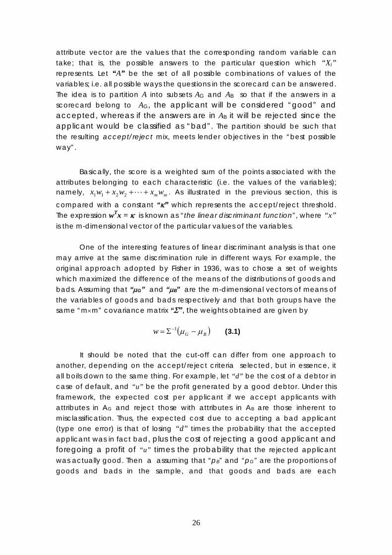
Basically, the score is a weighted sum of the points associated with the attributes belonging to each characteristic (i.e. the values of the variables); namely, . As illustrated in the previous section, this is

compared with a constant “κ” which represents the accept/reject threshold. The expression w

mmwxwxwx +⋅⋅⋅++ 2211

Tx = κ is known as “the linear discriminant function”, where “x” is the m-dimensional vector of the particular values of the variables. One of the interesting features of linear discriminant analysis is that one may arrive at the same discrimination rule in different ways. For example, the original approach adopted by Fisher in 1936, was to chose a set of weights which maximized the difference of the means of the distributions of goods and bads. Assuming that “μG” and “μB” are the m-dimensional vectors of means of the variables of goods and bads respectively and that both groups have the same “m×m” covariance matrix “Σ”, the weights obtained are given by

( )BGw μμ −Σ= −1 (3.1)

It should be noted that the cut-off can differ from one approach to another, depending on the accept/reject criteria selected, but in essence, it all boils down to the same thing. For example, let “d” be the cost of a debtor in case of default, and “u” be the profit generated by a good debtor. Under this framework, the expected cost per applicant if we accept applicants with attributes in AG and reject those with attributes in AB are those inherent to misclassification. Thus, the expected cost due to accepting a bad applicant (type one error) is that of losing “d” times the probability that the accepted applicant was in fact bad, plus the cost of rejecting a good applicant and foregoing a profit of “u” times the probability that the rejected applicant was actually good. Then a assuming that “p

B

BB” and “pG” are the proportions of goods and bads in the sample, and that goods and bads are each

26

multivariate, normally distributed with common covariance matrix as above, it can be shown that the cutoff which minimizes the expected cost is given by30,

.log2

1 1

⎟⎟⎠

⎞⎜⎜⎝

⎛××

+⋅−⋅

=∑ ∑− −

G

BBTBG

TG

pupdμμμμ

κ

From a geometric perspective, the hyperplane wTx = κ effectively divides or separates the set “A” of all possible values of the variables into two subsets; namely those of accepted applications (assumed to be “goods”) and that of the rejects (assumed to be “bads”); this is depicted in figure (2.1). Note that necessarily, there will be “goods” and “bads” in both subsets, due to uncertainty. As previously mentioned, the hyperplane derived from the previous analysis, ensures that the mixture of misclassified applicants (i.e. goods that are rejected and bads that are accepted) is optimal for several accept/reject criteria.

Accepts κ≥xwT

Rejects κ⟨xw T

2x

1x

κ=xwT

κ=xwT

Figure 3.1. The geometry of the accept/reject rule.

A particularly practical approach to obtaining the discriminant function is through linear regression, since the regression equations can be set up so that scores can be viewed as default probabilities. Formally, if “qi” is the probability that applicant i in the sample is a “good”, the regression equations are simply

mimiioi wxwxwxwq +⋅⋅⋅+++= 2211 for all i, (3.2) Thus, the probability of default is simply pi = 1 – qi. These expressions seem to correspond to continuous values of the variables but, as seen in the simple

30 See appendix A.

27

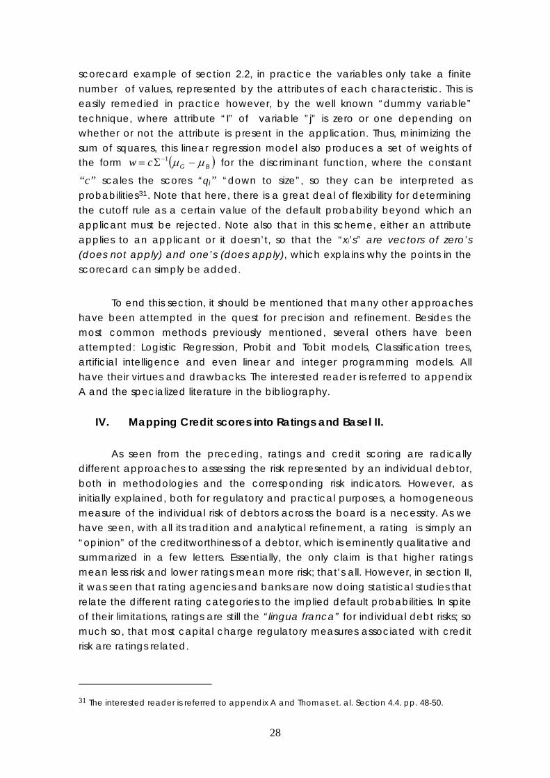
scorecard example of section 2.2, in practice the variables only take a finite number of values, represented by the attributes of each characteristic. This is easily remedied in practice however, by the well known “dummy variable” technique, where attribute “I” of variable ”j” is zero or one depending on whether or not the attribute is present in the application. Thus, minimizing the sum of squares, this linear regression model also produces a set of weights of the form ( )BGcw μμ −Σ= −1 for the discriminant function, where the constant

“c” scales the scores “qi” “down to size”, so they can be interpreted as probabilities31. Note that here, there is a great deal of flexibility for determining the cutoff rule as a certain value of the default probability beyond which an applicant must be rejected. Note also that in this scheme, either an attribute applies to an applicant or it doesn’t, so that the “xi’s” are vectors of zero’s (does not apply) and one’s (does apply), which explains why the points in the scorecard can simply be added.

To end this section, it should be mentioned that many other approaches have been attempted in the quest for precision and refinement. Besides the most common methods previously mentioned, several others have been attempted: Logistic Regression, Probit and Tobit models, Classification trees, artificial intelligence and even linear and integer programming models. All have their virtues and drawbacks. The interested reader is referred to appendix A and the specialized literature in the bibliography.

IV. Mapping Credit scores into Ratings and Basel II.

As seen from the preceding, ratings and credit scoring are radically different approaches to assessing the risk represented by an individual debtor, both in methodologies and the corresponding risk indicators. However, as initially explained, both for regulatory and practical purposes, a homogeneous measure of the individual risk of debtors across the board is a necessity. As we have seen, with all its tradition and analytical refinement, a rating is simply an “opinion” of the creditworthiness of a debtor, which is eminently qualitative and summarized in a few letters. Essentially, the only claim is that higher ratings mean less risk and lower ratings mean more risk; that’s all. However, in section II, it was seen that rating agencies and banks are now doing statistical studies that relate the different rating categories to the implied default probabilities. In spite of their limitations, ratings are still the “lingua franca” for individual debt risks; so much so, that most capital charge regulatory measures associated with credit risk are ratings related.

31 The interested reader is referred to appendix A and Thomas et. al. Section 4.4. pp. 48-50.

28

A particular case in point, is the “Standardized Approach” for capital requirements in the recent Basel II accord which in summary stipulates the Credit Risk Capital Requirement as 8% of the sum of the risk weighted assets; that is:

RWACRCR ×= %8

CRCR = Credit Risk Capital Requirement.

RWA = Sum of the Risk Weighted Assets along all segments of the portfolio.

If banks adopt the standardized approach, then:

∑=

=×=m

jjj wLRWACRCR

108.0%8

Where:

Lj = Total credit extended to segment “j”.

wj = Risk Weight for credit extended to segment “j”.

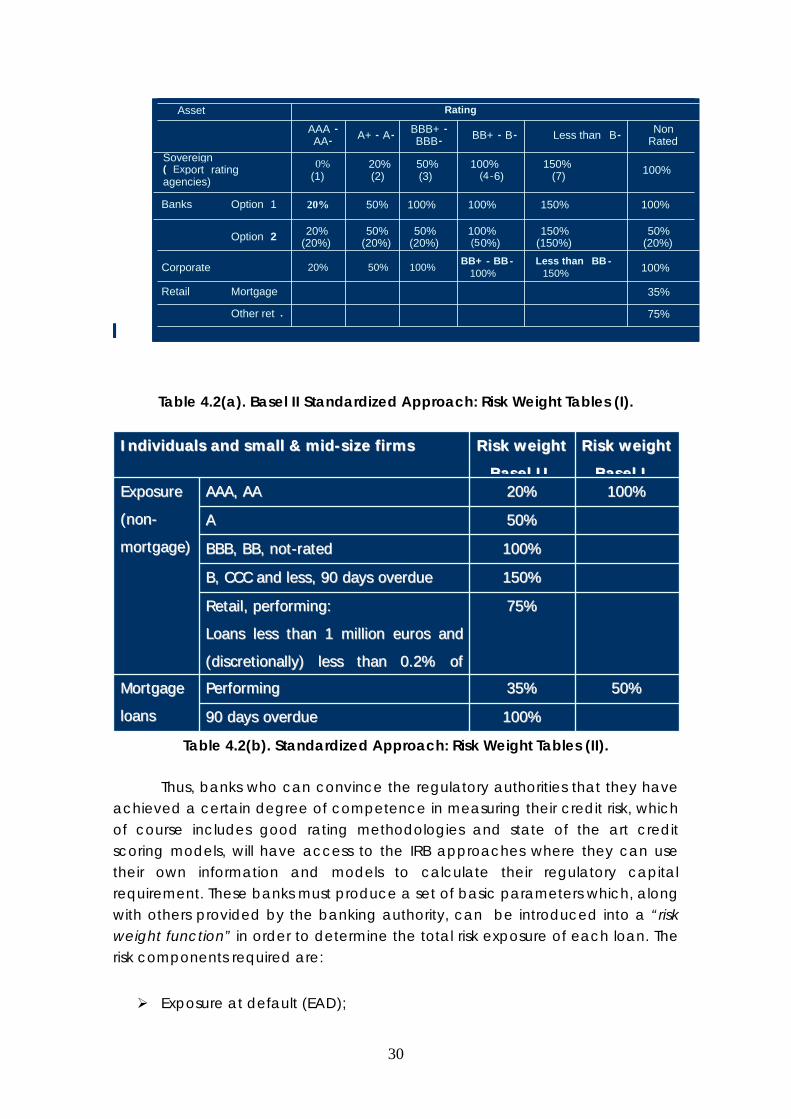
and they must strictly adhere to the risk weights proposed by the new accord, as shown in tables 4.2(a) and 4.2(b), which can be seen to be completely ratings driven. The standardized approach, proposes a separate framework for retail, project finance and equity exposures, and one of the main innovations (relative to the previous accord), is the use of ratings given by external rating agencies to set the risk weights for corporate, bank and sovereign claims. Note that these tables define “buckets” of ratings for different types of loans which establish a correspondence between specific ratings and regulatory capital weights.

Now the Basel II accord gives two other alternatives so that besides the standardized approach, the risk weights can be obtained by more precise and complex credit risk models, known as the “Internal Ratings Based” (IRB) approaches. The intention is that a hierarchy should be established for the capital requirements under the three proposed alternatives; namely: That the capital requirement by the “standardized approach” is larger than under the “foundations internal ratings based(IRB)” approach, which is in turn greater than the requirement under “the advanced IRB approach”. The bigger the differences, the larger the incentives for banks to invest in better risk management tools.

29

Asset Rating

AAA -AA- A+ - A- BBB+ -

BBB- BB+ - B- Less than B- Non Rated

Sovereign( Export ratingagencies)

0%(1)

20%(2)

50%(3)

100%(4-6)

150%(7) 100%

Banks Option 1 20% 50% 100% 100% 150% 100%

Option 2 20%(20%)

50%(20%)

50%(20%)

100%(50%)

150%(150%)

50%(20%)

Corporate 20% 50% 100% BB+ - BB -100%

Less than BB -150% 100%

Retail Mortgage 35%

Other ret . 75%

Asset Rating




0%(1)

20%(2)

50%(3)

100%(4-6)

150%(7) 100%

Banks Option 1 20% 50% 100% 100% 150% 100%

Option 2 20%(20%)

50%(20%)

50%(20%)

100%(50%)

150%(150%)

50%(20%)

Corporate 20% 50% 100% BB+ - BB -100%


Retail Mortgage 35%

Other ret . 75%

Asset Rating




0%(1)

20%(2)

50%(3)

100%(4-6)

150%(7) 100%

Asset Rating




0%(1)

20%(2)

50%(3)

100%(4-6)

150%(7) 100%

Banks Option 1 20% 50% 100% 100% 150% 100%

Option 2 20%(20%)

50%(20%)

50%(20%)

100%(50%)

150%(150%)

50%(20%)

Banks Option 1 20% 50% 100% 100% 150% 100%

Option 2 20%(20%)

50%(20%)

50%(20%)

100%(50%)

150%(150%)

50%(20%)

Corporate 20% 50% 100% BB+ - BB -100%


Retail Mortgage 35%

Corporate 20% 50% 100% BB+ - BB -100%


Retail Mortgage 35%

Other ret . 75%

Table 4.2(a). Basel II Standardized Approach: Risk Weight Tables (I).

110000%% 9900 ddaayyss oovveerrdduuee

5500%% 3355%% PPeerrffoorrmmiinngg MMoorrttggaaggee

llooaannss

7755%% RReettaaiill,, ppeerrffoorrmmiinngg::

LLooaannss lleessss tthhaann 11 mmiilllliioonn eeuurrooss aanndd

((ddiissccrreettiioonnaallllyy)) lleessss tthhaann 00..22%% ooff

115500%% BB,, CCCCCC aanndd lleessss,, 9900 ddaayyss oovveerrdduuee

110000%% BBBBBB,, BBBB,, nnoott--rraatteedd

5500%% AA

110000%% 2200%% AAAAAA,, AAAA EExxppoossuurree

((nnoonn--

mmoorrttggaaggee))

RRiisskk wweeiigghhtt

BBaasseell II

RRiisskk wweeiigghhtt

BBaasseell IIII

IInnddiivviidduuaallss aanndd ssmmaallll && mmiidd--ssiizzee ffiirrmmss

Table 4.2(b). Standardized Approach: Risk Weight Tables (II).

Thus, banks who can convince the regulatory authorities that they have achieved a certain degree of competence in measuring their credit risk, which of course includes good rating methodologies and state of the art credit scoring models, will have access to the IRB approaches where they can use their own information and models to calculate their regulatory capital requirement. These banks must produce a set of basic parameters which, along with others provided by the banking authority, can be introduced into a “risk weight function” in order to determine the total risk exposure of each loan. The risk components required are:

Exposure at default (EAD);

30

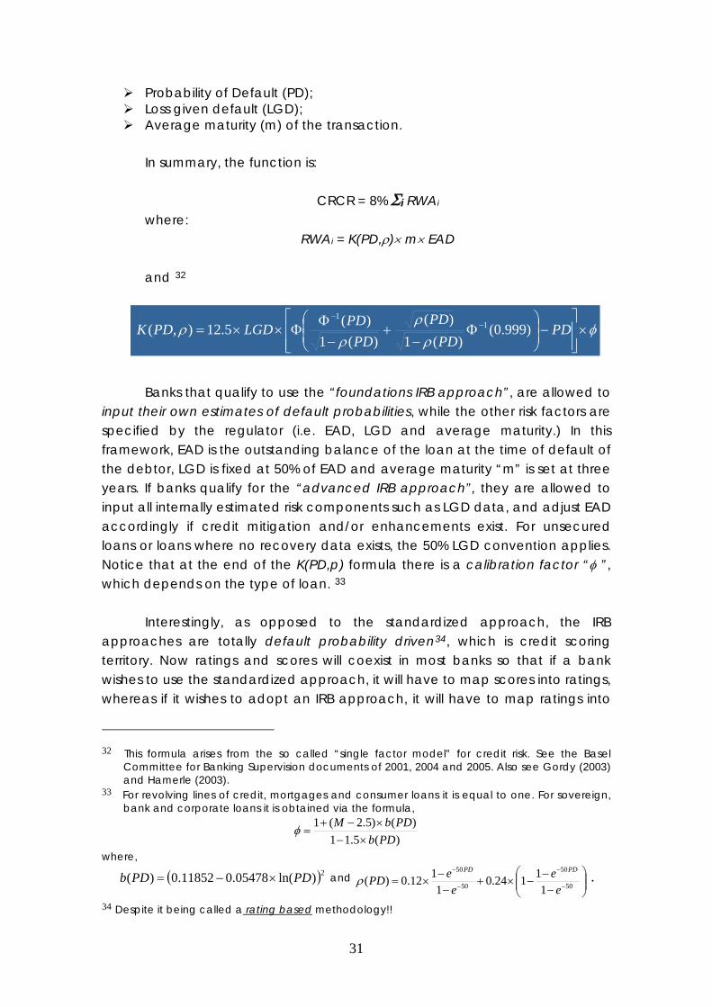
Probability of Default (PD); Loss given default (LGD); Average maturity (m) of the transaction.

In summary, the function is:

CRCR = 8% Σi RWAi

where: RWAi = K(PD,ρ)× m× EAD

and 32

Banks that qualify to use the “foundations IRB approach”, are allowed to

input their own estimates of default probabilities, while the other risk factors are specified by the regulator (i.e. EAD, LGD and average maturity.) In this framework, EAD is the outstanding balance of the loan at the time of default of the debtor, LGD is fixed at 50% of EAD and average maturity “m” is set at three years. If banks qualify for the “advanced IRB approach”, they are allowed to input all internally estimated risk components such as LGD data, and adjust EAD accordingly if credit mitigation and/or enhancements exist. For unsecured loans or loans where no recovery data exists, the 50% LGD convention applies. Notice that at the end of the K(PD,p) formula there is a calibration factor “φ ”, which depends on the type of loan. 33

Interestingly, as opposed to the standardized approach, the IRB

approaches are totally default probability driven34, which is credit scoring territory. Now ratings and scores will coexist in most banks so that if a bank wishes to use the standardized approach, it will have to map scores into ratings, whereas if it wishes to adopt an IRB approach, it will have to map ratings into

φρ

ρρ

ρ ×⎥⎥⎦

⎤

⎢⎢⎣

⎡−⎟

⎟⎠

⎞⎜⎜⎝

⎛Φ

−+

−Φ

Φ××= −−

)999.0()(1

)()(1

)(5.12),( 11

PDPD

PDPD

PDLGDPDK

32 This formula arises from the so called “single factor model” for credit risk. See the Basel

Committee for Banking Supervision documents of 2001, 2004 and 2005. Also see Gordy (2003) and Hamerle (2003).

33 For revolving lines of credit, mortgages and consumer loans it is equal to one. For sovereign, bank and corporate loans it is obtained via the formula,

)(5.11)()5.2(1

PDbPDbM

×−×−+

=φ

where,

( )2)ln(05478.011852.0)( PDPDb ×−= and ⎟⎟⎠

⎞⎜⎜⎝

⎛−−

−×+−−

×= −

−

−

−

50

50

50

50

11124.0

1112.0)(

ee

eePD

PDPD

ρ .

34 Despite it being called a rating based methodology!!

31

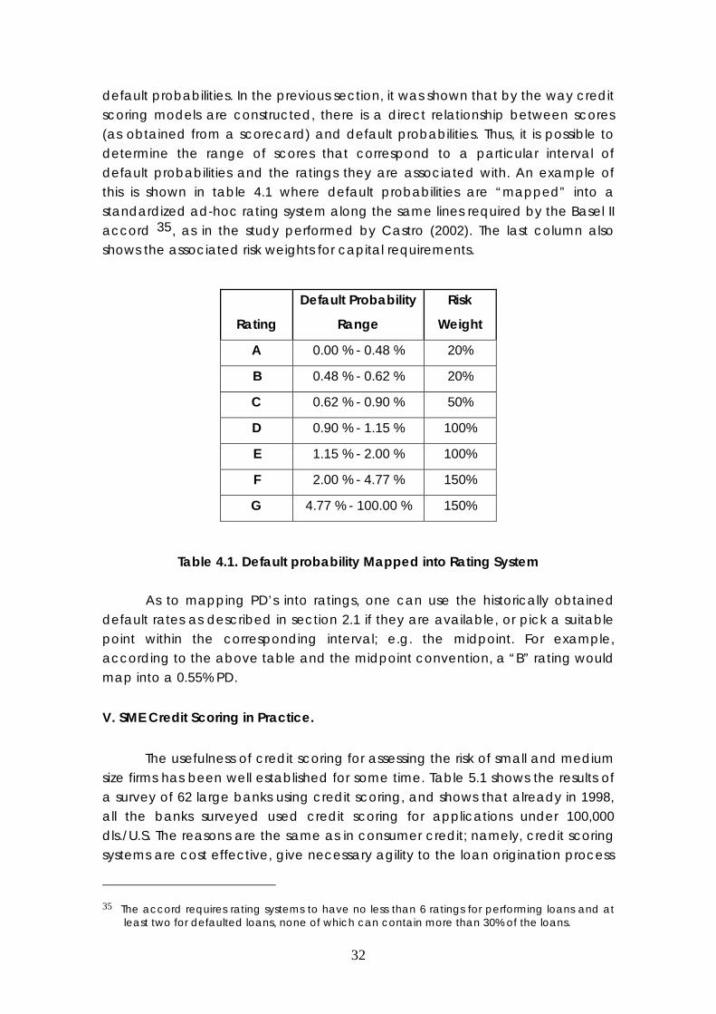
default probabilities. In the previous section, it was shown that by the way credit scoring models are constructed, there is a direct relationship between scores (as obtained from a scorecard) and default probabilities. Thus, it is possible to determine the range of scores that correspond to a particular interval of default probabilities and the ratings they are associated with. An example of this is shown in table 4.1 where default probabilities are “mapped” into a standardized ad-hoc rating system along the same lines required by the Basel II accord 35, as in the study performed by Castro (2002). The last column also shows the associated risk weights for capital requirements.

Rating

Default Probability

Range

Risk

Weight

A 0.00 % - 0.48 % 20%

B 0.48 % - 0.62 % 20%

C 0.62 % - 0.90 % 50%

D 0.90 % - 1.15 % 100%

E 1.15 % - 2.00 % 100%

F 2.00 % - 4.77 % 150%

G 4.77 % - 100.00 % 150%

Table 4.1. Default probability Mapped into Rating System

As to mapping PD’s into ratings, one can use the historically obtained default rates as described in section 2.1 if they are available, or pick a suitable point within the corresponding interval; e.g. the midpoint. For example, according to the above table and the midpoint convention, a “B” rating would map into a 0.55% PD.

V. SME Credit Scoring in Practice.

The usefulness of credit scoring for assessing the risk of small and medium size firms has been well established for some time. Table 5.1 shows the results of a survey of 62 large banks using credit scoring, and shows that already in 1998, all the banks surveyed used credit scoring for applications under 100,000 dls./U.S. The reasons are the same as in consumer credit; namely, credit scoring systems are cost effective, give necessary agility to the loan origination process

35 The accord requires rating systems to have no less than 6 ratings for performing loans and at

least two for defaulted loans, none of which can contain more than 30% of the loans.

32

and facilitate data collecting in a systematic way. The data collected on applicants and clients can be fed back into the process and add much value over time, in the form of progressively better models with more discriminatory power which ultimately result in better default probability estimation, valuation and overall risk assessment capabilities; both for new, through the door applicants, and existing accounts.

Number Percent of

Scoring Banks

Loan Sizes Scored

Under $100,000 62 100.0

$100,000 - $250,000 46 74.2

$250,000 - $1,000,000 13 21.0

Automatic Approval/Rejection 26 41.9

Setting Loan Terms 20 32.3

Use of Proprietary Models 8 12.9

Average Number of Months 24 ---

Table 5.1: Survey Results for Large U.S. Banks Using Small Business Credit Scoring Data as of January 31, 1998ª

ªSource: Frame, Srinivasan, and Woosley (2001).

The table also shows that banks do not find credit scoring equally useful in all cases; in particular, as the size of the requested loan and/or soliciting firm increases, credit scoring is used less and less. Thus, the most successful application of CS models is in the lower bracket of SME’s, because much of the relevant data is on the personal characteristics of the owners, which in this case has good predictive power of the performance of the loan. As you go up the spectrum into larger SME's, the business (market, competition, financials etc.)characteristics of the SME's begin to outweigh those of the owners, becoming very important in the top bracket. In fact, banks treat large SME's (Assets around 6 million U.S. dls. in Mexico) pretty much the same way they will any large company. In summary, the characteristics that have explanatory power change with the size of the company. To this authors knowledge, in the case of larger SME’s, the banks which have the capability to do so, apply the questionnaire only as an initial filter, since they are only accurate for outright rejection.

There are two significant obstacles to applying credit scoring models to larger SME’s. The first is the problem of “opacity”; that is, obtaining hard

33

information in terms of “quality” (i.e. accuracy and credibility), relevance, and the ease with which it can be used in a systematic way. As mentioned above, financial statement information becomes increasingly important in the process, but it is not uniformly reliable over all SME’s. Because they don’t issue debt or stocks which can be scrutinized by analysts and rating agencies, audited financial statements are not common, since businesses are not required to keep reliable records; much less provide them to the public. Thus, the typical scorecard for SME’s, contain more characteristics which describe the owners, and their payment histories on their personal loans, than financial data on their businesses. This is particularly true on the lower end of the spectrum, where businesses are fairly simple and the owners see no need to keep very accurate financial statements. Although this may improve with the size of the firms, softer data on the nature of the business and the quality of the management, which are difficult to capture and standardize become more important, and so far have defied systematization at the high end of the spectrum. As mentioned by Berger and Frame (2007), banks are compensating for the opacity problem by resorting to “relationship lending”; i.e. the debtors history with the bank. Gathering useful relationship data on clients, which can be used in credit scoring models is a slow process, because much of the data is not easily observable, and it is difficult to validate and make it “hard enough”, so that it can be used in a scorecard. The second obstacle to applying credit scoring to large SME’s is structural in nature. One must keep in mind that credit scoring thrives in large populations, whose members can be described by the same set of common characteristics, where statistical techniques can be precise. As one moves up the scale, the population of firms starts thinning down rapidly; from thousands to hundreds to only a few. The problem is aggravated by the heterogeneity of the business sectors where they carry out their activities.36 Both these issues contribute to making the usefulness of credit scoring in the higher brackets of SME´s very questionable if not impossible. In section 3.3.1, on sampling, recall that the referenced authors recommended sample sizes between 3000 and 4000 debtors; with equal proportions of goods and bads. What sense does this make if the total population is a few hundred or maybe a dozen companies? To top it off, what may be a healthy financial ratio in a certain sector may be total nonsense or even disastrous in another; again the problem of different characteristics to explain defaults in different sectors. Besides narrowing down the populations even further, it makes it impossible to obtain a set of homogenous characteristics which make any sense!!

36 In Mexico for example, there are complete industrial sectors represented by only one

company!

34

VI. Concluding Remarks.

Although addressing the same problem of assessing individual credit risk, we have argued that whereas ratings are based on the techniques of fundamental analysis and are applied to asses the default risk of large companies, credit scoring is a scientific approach which is applied to large populations of small debtors where defaults can be explained by the same homogenous set of characteristics. This however does not mean that no relationship can be found between the two; this is not only possible but necessary. In section IV it was seen that the default probabilities, although obtained in very different ways, provide the necessary means of relating one to the other. Furthermore, both ratings and scores can be used for regulatory purposes, and in particular, can be applied in Basel II.

As regards SME’s, we have argued that credit scoring has been

successfully used at the lower end of the spectrum for many years, but its usefulness decreases as we move up the scale; both due to the difficulty of obtaining sufficiently reliable information, and structurally, because populations decrease rapidly as size increases, so that it is difficult to obtain good samples on which to calibrate the models. This problem is further aggravated by the heterogeneity of small companies, whose defaults can therefore not be explained by the same set of characteristics, making it impossible in some cases to get any kind of a sample for estimating a credit scoring model. Thus, as the size of the SME’s increases, the output from credit scoring models is subject to increasing interpretation by traditional analysts who can, at anytime, override the systems recommendation. Thus as size increases, the assessment of credit risk relies ever more on traditional credit analysts and less on automated scoring methods, which are practically ignored for large SME’s.

Finally, although the discussion is well beyond the scope of this paper, it is

important to have a clear idea of the role of credit scoring in the general SME credit context. In particular, it would be unfair to place a big responsibility for the growth of credit in the SME market, squarely on the shoulders of credit scoring. This authors enquiries so far have evidenced that, even if everybody had good models, that allowed a rapid response to all SME loan petitions, this would be insufficient to stimulate rapid growth. In summary, there are important obstacles apart from the problems of agile response and standardized and hard reliable information, that range from fiscal and regulatory issues to the availability of adequate banking products for the market; even cultural characteristics in different countries can provide negative incentives and become important obstacles to SME credit growth. Hopefully these issues will be addressed in further studies and research.

35

Appendix A: Discriminant Analysis

A.1. The Decision Theoretical Approach.

In this approach, it is assumed that the penalties for misclassification of

applicants can be quantified in homogeneous units, and the objective is to

partition A = AG ∪ AB so that the expected penalty to the lender is minimized.

Thus, without loss of generality, and in the simplest case, assume that the

expected profit is the same for all applicants and is denoted by “u”. Assume

also, that the loss in case of default is the same for any accepted applicant

and is denoted by “d”.

B

Let pG denote the proportion of applicants that are “good” and pB

denote the proportion of those that are “bad”. Then the theory of conditional

probability tells us that the probability that a good applicant has attributes “x”

is:

( ) .)(Pr

)(Prgoodisapplicantob

xattibuteshasandgoodisapplicantobGxp = (A.1)

Similarly, let ( Bxp ) denote the probability that a bad applicant will have

attributes “x”.

If ( xGq ) denotes the probability that someone with attributes x is a good

applicant, then,

( ) ,)(Pr

)(Prxattibueshasapplicantob

goodisandxattributeshasapplicantobxGq = (A.2)

and if then (2.1) and (2.2) can be

rearranged to read

( ) x)attributes hascant Prob(appli=xp

( ) ( ) ( ) . good) is and x attributes hascant Prob(appli GpGxpxpxGq == (A.3)

36

From Baye’s theorem, we have that

( ) ( )( ) .xp

pGxpxGq G= (A.4)

Similarly, if ( xBq ) is the probability that someone with attributes x is a bad

applicant, then,

( ) ( )( ) .xp

pBxpxBq B= (A.5)

Solving for “p(x)” in (2.4) and (2.5), equating and rearranging terms, leads to

( )( )

( )( ) .

B

G

pBxppGxp

xBqxGq= (A.6)

Under this framework, the expected cost per applicant if we accept

applicants with attributes in AG and reject those with attributes in AB are those

inherent to misclassification. Thus, the expected cost due to accepting a bad

applicant (type one error) is that of losing “d” with probability

B

( xBq ) when x

belongs to AG, plus the cost of rejecting a good applicant and foregoing

a profit of “u” with probability ( )xGq with x belonging to ABB. In other words,

if we categorize a particular set of attributes ( )pxxxx ,...,, 21= into AG, then there

is only a cost if it is a bad, in which case the expected cost is ( ) BpBxpd × . If x is

classified into AB, there is only a cost if it is a good, and so the expected cost is B

( ) GpGxpu × . By the laws of expectation, adding up over all possible “x”, and

since goods and bads are in proportions pG and pBB respectively, the expected

penalty per debtor is:

37

( ) ( ) ( ) ( ) ( ) ( )∑∑∑∑∈∈∈∈

+=+GBGB AxAxAx

BAx

G xpxBqdxpxGqupBxpdpGxpu .

(2.7)

The rule that minimizes this expected cost is straightforward. Retaking the

above, one classifies x into AG only if the expected profit of so doing is greater

than the penalty for misclassification; i.e. if ( ) ( ) GB pGxpupBxpd ×≤× . Thus,

from (2.6), the classification rule that minimizes the expected cost is given by

( ) ( ){ } ( )( )

( )( )⎪⎭

⎪⎬⎫

⎪⎩

⎪⎨⎧

≤=⎪⎭

⎪⎬⎫

⎪⎩

⎪⎨⎧

≤=×≤×=xBqxGq

udx

pBxppGxp

uxpGxupBxpdxAB

GGBG (A.8)

As previously mentioned, applicants are classified as Bad if they can’t be

classified as good, so that AB is simply the complement of AB G.

The above classification rule depends on being able to estimate “u” and

“d” or their ratio, which may not be possible. If this is the case, a reasonable

alternative is to minimize the probability of committing one type of error while

fixing the probability of committing the other at an acceptable level. The

obvious thing to do is to minimize the losses due to default (type one error) while

maintaining the percentage of accepted applicants at some pre-established

level, which is equivalent to keeping the probability of rejecting good

applicants (type two error) at a certain level. To formalize this, let “a” denote

the desired acceptance rate (i.e. percentage of accepted through the door

applicants). Then AG is the subset of A which minimizes the expected default

rate ( )∑∈ GAx

BpBxp , subject to the constraint

( ) ( )∑∑∈∈

=+GG Ax

BAx

G apBxppGxp (A.9)

If we define ( ) ( ) BpBxpxb = for each Ax∈ , the optimization problem is more

conveniently written as

38

Minimize ( ) ( )( ) ( )∑∑

∈∈⎟⎟⎠

⎞⎜⎜⎝

⎛=

GG AxAxxp

xpxbxb subject to ( ) axp

GAx∑∈

= 37 (A.10)

Playing the Lagrange multiplier game, the optimal AG must be the set of

attributes x satisfying ( )( ) cxpxb

≤ , where c is a constant such that the sum of the

p(x) that satisfy 2.9 is equal to a. From the definitions of p(x) and b(x)and

relationships 2.4, 2.5 and 2.6, after a bit of algebra, one arrives at the following

expression:

( )( )

( )( ) ⎪⎭

⎪⎬⎫

⎪⎩

⎪⎨⎧

≤−

=⎭⎬⎫

⎩⎨⎧

≤=B

GG pBxp

pGxpc

cxcxpxbxA 1

(A.11)

Note that this is virtually the same decision rule as (2.8), and that (1-c)/c is

the implicit D/L ratio in the type one error minimization criteria. 38

Replacing conditional distribution functions ( ) ( )BxpGxp , by conditional

density functions ( ) ( BxfGxf , ) and summation signs by integrals, one can

obtain the same results for continuous variables by playing the same game.

The corresponding decision rule that minimizes the expected cost for

continuous variables is then:

( ) ( ){ } ( )( )⎪⎩

⎪⎨⎧

⎪⎭

⎪⎬⎫

≤=≤= .BxfGxf

updpxpGxufpBxdfxA

G

BGBG (A.12)

37 To see this note that ( ) ( ) ( ) B

AxB

AxB

Ax

pBxppBxppBxpBG

∑∑∑∈∈∈

+= and from 2.4 and 2.5

obtain ( ) ( ) ( ) BG pBxppGxpxp += etc.

38 In other words, type one error minimization implicitly assigns a loss given default to foregone

profit ratio (d/u) equal to (1-c)/c.

39

A.2. Finding weights assuming “goods” and “bads” each have Multivariate

normal distributions with common covariance

In order to apply the decision theoretical approach directly, the only

thing that remains is to specify particular distribution functions for good and

bad applicants. Although theoretically there is no limitation, in practice one

would like to have distributions which can be easily manipulated. An obvious

candidate is the multivariate Normal distribution. Thus, assume there are “n”

characteristics or variables in the scorecard, and the random outcomes of

goods and bads are adequately characterized by multivariate normal

distributions. For convenience, in this section characteristics will always be

called variables and matrix notation is used throughout. All vectors are “column

vectors” so that an “m-dimensional vector” is a matrix with one column and

“m” rows and the transpose of a vector is denoted with the superscript “T”.

Thus, “x” is an m-dimensional vector denoting particular values of the variables

and μG and μB are the m-dimensional vectors of means of the variables of

goods and bads respectively. Assume both groups have the same “m×m”

covariance matrix 39

B

∑ . This means that ( ) ( ) ,,,, iBiiGi BXEGXE μμ == and

( ) ( ) .∑==ijjiji BXXEGXXE .

The corresponding density functions for goods and bads in this case are

( ) ( ) ( ) ( ),

2exp2

1

21

22

⎟⎟⎟

⎠

⎞

⎜⎜⎜

⎝

⎛ −−−Σ=

∑−

−−

T

GGp xxGxf

μμπσ (A.13a) and

( ) ( ) ( ) ( ),

2exp2

1

21

22

⎟⎟⎟

⎠

⎞

⎜⎜⎜

⎝

⎛ −−−Σ=

∑−

−−

T

BBp xxBxf

μμπσ (A.13b)

39 The reader interested in examining the case where the covariance matrices are different for

goods and bads is referred to Thomas et. al. Ch. 4. However, it should be pointed out that the

added uncertainty inherent in estimating two covariance matrices instead of one, makes the

ensuing “quadratic” decision rule less robust than the linear one, and the slightly better

accuracy is not worth the effort in general.

40

Where ( Gx )μ− is a vector and ( )TGx μ− is its transpose, which is the same set

of numbers represented as a vector with “n” rows and 1 column. Recall that

decision rule(2.12) states that

( )( ) G

B

updp

BxfGxf

≥

And substituting (2.13a) for goods in the numerator and (2.13b) for bads in the

denominator, a bit of algebra leads to

( )∑∑ ∑−

− −

⎟⎟⎠

⎞⎜⎜⎝

⎛+

⋅−⋅≥−⋅

1

1 1

.log2 G

BBTBG

TG

BGT

updp

xμμμμ

μμ (A.14)

Thus, the left-hand side of (2.14) is a weighted sum of the values of the

variables, namely, mmwxwxwx +⋅⋅⋅++ 2211 , while the right-hand side is a

constant which represents the accept/reject threshold. Expression (2.14) is

known as “the linear discriminant function”, and the n-dimensional vector of

“weights” of the values of the variables is given by,

( )BGw μμ −Σ= −1 (A.15)

whereas the cut-off constant is:

.log2

1 1

⎟⎟⎠

⎞⎜⎜⎝

⎛+

⋅−⋅=

∑ ∑− −

G

BBTBG

TG

LpDpμμμμ

κ (A.16)

In practice, the means and covariance’s of the distributions are

unknown, so they are replaced by their estimates, namely, the sample means

and and the sample covariance matrix S. With this notation (2.14)

some authors prefer to write the rule as:

Gm Bm

( ) .log2

111

⎟⎟⎠

⎞⎜⎜⎝

⎛+

⋅−⋅≥−⋅

−−−

G

BTBB

TGGT

BG LpDpmSmmSm

mmSx (A.15)

41

A.3. Discriminant analysis: A form of linear regression

It should be pointed out that one may arrive at the same discrimination

rule in different ways. For example, the original approach adopted by Fisher in

1936, was to chose a set of weights which maximized the difference of the

means of the distributions of goods and bads. Perhaps surprisingly, doing so

produces exactly the same set of weights with the advantage that no

distributional assumptions are made.40 Although the derivation of the decision

rule of the previous section is very elegant and intuitively appealing, it is obvious

that in practice it can be a bit awkward. A more practical approach to obtain

the discriminant function is through linear regression. Besides the fact that the

technique is easy to implement, the added attraction of this approach, is that

the regression is set up so that the linear combination of the variables Is that

which best explains the probability of default. Formally, if “qi” is the probability

that applicant i in the sample is a “good”, the regression equations are simply41

mimiioi wxwxwxwq +⋅⋅⋅+++= 2211 for all i, (A.16)

Let “nG” and “nB” be the number of goods and bads in the sample

respectively, so that the size of the sample is n =n

B

G + nBB, and without loss of

generality assume the first “nG” in the sample are the goods and the remaining

“nB” of the sample are bad. Therefore, in the regression equation, B

⎩⎨⎧

++==

=BGG

Gi nnnifor

niforq

,...,10,....,2,11

(A.17)

And the regression equations will be:

40 The interested reader can consult Thomas et. al. Ch. 4, section 4.3. 41 These expressions seem to correspond to continuous values of the variables, but in practice

the variables only take a finite number of values, represented by the attributes of each

characteristic. This is easily remedied in practice however, by the well known “dummy

variable” technique, where attribute “I” of variable ”j” is zero or one depending on whether

or not the attribute is present in the application.

42

BGGpimiio

Gpimiio

nnniforwxwxwxw

niforwxwxwxw

++=+⋅⋅⋅+++=

=+⋅⋅⋅+++=

,...,10

,....,2,11

2211

2211 (A.18)

In linear regression the optimization criterion is to minimize the mean

square error between the left-and right-hand sides of (2.18); i.e.

2

1 0

2

1 0.1 ∑ ∑∑ ∑

+

+= == =⎟⎟⎠

⎞⎜⎜⎝

⎛+⎟⎟

⎠

⎞⎜⎜⎝

⎛−

BG

G

G nn

ni

m

jijj

n

i

m

jijjw

xwxwMinimize (A.19)

Now, by the structure of the model and the rules of expectation, it can

be shown that this linear regression model also produces a set of weights of the

form for the discriminant function, where the constant “c”

scales the scores “q

( BGcw μμ −Σ= −1 )

i” “down to size”, so they can be interpreted as

probabilities42.

By construction, each score “qi” is the probability that an applicant is a

“good” and therefore will not default. In this vein, the probability of default of

an applicant will simply be the complement i.e. the default probability is pi = 1 -

qi. Note that here, there is a great flexibility for determining the cutoff rule as a

certain level value of the default probability beyond which an applicant must

be rejected.

A.4. Logistic regression.

Obviously, the main drawback of the regression approach is that the

score “qi” can be a number outside the unit interval [0, 1], thus failing to satisfy

a basic requirement for being a probability measure. One approach to correct

this problem is that of “logistic regression”, where the regression equations are

of the form:

42 The interested reader is referred to Thomas et. al. Section 4.4. pp. 48-50.

43

xwxwxwxwwq

q Tppo

i

i =++++=⎟⎟⎠

⎞⎜⎜⎝

⎛−

L22111log (A.20)

If qi ≥ 0 then i

i

qq−1

takes on values between 0 and +∞, and log ⎟⎟⎠

⎞⎜⎜⎝

⎛− i

i

qq

1 takes

values between -∞ and +∞. By the rules of logarithms, solving for qi produces

xw

xw

i eeq ⋅

⋅

+=

1 (A.21)

which is the well known “logistic regression assumption”, and it is clear that 0 <

qi < 1. Under the assumption that the distributions of the characteristic values of

the goods and bads are multivariate normal’s with common covariance

matrices, logistic regression also produces a linear discriminant function.

An important consideration however, is that there are many other

distributions which also satisfy the logistic assumption, and could theoretically

produce discriminant functions with better classification power. Besides leading

to non-linear discriminant functions, which effectively goes against the simplicity

of additive scorecards, and although modern computing technology is well up

to the task, there is an added difficulty since weights must be estimated by

maximum likelihood techniques, which in turn requires the use of a numerical

optimization procedure (e.g. the Newton-Raphson method). Furthermore, linear

and logistic regression have been compared exhaustively in practice, and the

empirical evidence obtained by applying both techniques to the same set of

data shows that both methods produce very similar results. There is a theoretical

explanation however, since it can be shown that “q” and log[q/(1-q)] behave in

a very similar way, except when “q” is close to its extreme values; zero and one.

Note however that whatever the related scores are in these extremes, these

pertain to applicants whose behavior is easily predictable, whereas in the other

regions where classification is less evident, the two curves approximate each

other very closely, thus explaining why there is very little difference in the way

they classify applicants.

44

Bibliography.

E. I. Altman (1968), “Financial Ratios, Discriminant Analysis and the Prediction of Corporate Bankruptcy”, Jnl. of Finance, 23, pp. 589-609.

Altman, E.I. (1977): “Zeta Analysis, A New Model to Identify Bankruptcy Risk of Corporations.” Journal of Banking and Finance.

Altman, E.I. (1989): “Measuring Corporate Bond Mortality and Performance.” The Journal of Finance.

Altman E.I., and D.L. Kao. (1992ª). “Rating Drift-Yield Bonds”. Journal of Fixed Income (March).

Altman, E.I., and V.M. Kishore. (1997). “Defaults and Return on High Yield Bonds: Analysis Through 1996”. Special report, New York University Salomon Center, New York, N.Y.

Basel Committee on Banking Supervision (BCBS) (2001), The Internal Ratings-Based Approach. Supporting Document to the New Basel Capital Accord. Consultative Document. Basel Committee on Banking Supervision (BCBS) (2004), Basel II: International Convergence of Capital Measurement and Capital Standards: a Revised Framework. Basel Committee on Banking Supervision (BCBS) (2005), An Explanatory Note on the Basel II IRB Risk Weight Functions. Allen N. Berger and W. Scott Frame, 2007, “Small Business Credit Scoring and Credit Availability”. Jnl. of Small Business Management 45(1) pp. 5-22. N. Capon (1982), “Credit Scoring Systems: A critical analysis”, Jnl. Of Marketing 46, pp. 82-91. Carey, M., Hrycay, M., 2001. Parameterizing Credit Risk Models with Rating Data. Journal of Banking and Finance 25, 197-270. Castro, Christian (2002), “Aplicación del enfoque IRB para el sistema financiero

Argentino utilizando datos de la central de deudores”. Banco Central De la

Republica Argentina. Unpublished document.

G. A. Churchill, J.R. Nevin and R. R. Watson (1977) “The role of Credit Scoring in the Loan Decision”. Credit World, March, pp. 6-10.

45

G. A. Churchill and J.R. Nevin (1979), “The Equal Credit Opportunity Act: An evaluation”, Jnl. Of Marketing, 42, pp. 95-104. Cuena Bartolomé, José, Ana García-Serrano and Javier Márquez Diez-Canedo (1990): "CYRCE: A Pattern of Knowledge Representation and Knowledge Acquisition for Decision on Personal Loans", Expert Systems with applications Vol. 1 pp 155-160 Pergamon Press pic. D. Durand(1941), “Risk elements in Consumer Installment financing”, National Bureau of Economic Research, New York. Equal Credit Opportunity Act (1975), United States Code, Title 15, Section 1691, et. Seq. Equal Credit Opportunity Act Amendments of 1976 (1976), “Report of the Committee on Banking, Housing and Urban Affaires, 94th. Congress, U.S. Government Printing Office, Washington D.C. R. A. Fisher(1936), “The use of multiple measurements in taxonomic problems”. Ann. Eugenics, 7, 179-188. Frame, W. Scott, Aruna Srinivasan, and Lynn Woosley (2001). “The Effect of

Credit Scoring on Small Business Lending.” Journal of Money, Credit, and

Banking, 33, 813-825

Gordy, M. B. (2003).”A risk-factor model foundation for ratings-based bank capital rules,” Journal of Financial Intermediation 12, 199-232. Hamerle, A., Liebig, T., Rösch, D., 2003. Credit Risk Factor Modeling and the Basel II IRB Approach. Discussion Paper Series 2: Banking and Financial Supervision, No 02/2003, Deutsche Bundesbank. Hopper, M.A. and E.M. Lewis (2002), “Behavior scoring and adaptive control systems.”; Credit Scoring and Credit Control (Thomas, Crook, and Edelman eds.) pp. 257-76, Oxford. E. M. Lewis (1992), “An introduction to credit scoring”. Athena Press, San Rafael, Calif. J.H. Myers and E. W. Forgy (1963) “The development of numerical credit evaluation systems”. Jnl. of the American Statistical Association, 58, pp.799-806.

46

A. K. Reichert, C. C. Cho and G. M. Wagner (1983): “An examination of the conceptual issues involved in developing credit scoring models”. Jnl. of Business, Econom. Statist. , 1, pp. 101-114. A. Saunders (1985), “This is Credit Scoring”, Credit Management, Sept. pp. 23-26. Naeem Siddiqi (2006), “Credit Risk Scorecards: Developing and Implementing Intelligent Credit Scoring”. John Wiley & Sons Inc. L. C. Thomas, D. B. Edelman and J. N. Crook (2002): “Credit Scoring and its Applications”; SIAM Monographs on Mathematical Modeling and Computation. E. F. Wonderlic (1952), “An analysis of factors in granting credit”, Indiana University Bulletin, 50, pp. 163-176.

47

Introduction to Credit Scoring · the principle of “the investor's right to know.” In 1860...

Documents

Transcript of Introduction to Credit Scoring · the principle of “the investor's right to know.” In 1860...