Introduction to COMSOL

Travis CampbellDeveloped for CHE 331 – Fall 2012

Oregon State UniversitySchool of Chemical, Biological and Environmental Engineering

What is COMSOL?

• Course requirement

• Modeling and simulation software

• Tool for system design/optimization

• Method for checking work

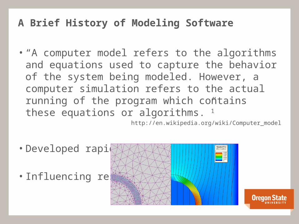
A Brief History of Modeling Software

• “A computer model refers to the algorithms and equations used to capture the behavior of the system being modeled. However, a computer simulation refers to the actual running of the program which contains these equations or algorithms.”1

http://en.wikipedia.org/wiki/Computer_model

• Developed rapidly with computers

• Influencing research

The General Idea Behind Numerical Modeling

• User builds a model with significant variables

• User builds a model mesh

• COMSOL solves the model numerically at every mesh intersection

• Intersections are connected to provide “continuous” data

How is the model solved at every intersection?

• Several methods exist - one example is the Finite Element Method:

𝑆𝑜𝑙𝑣𝑒𝑑𝑦𝑑𝑥

=2𝑥 h𝑤𝑖𝑡 𝑜𝑢𝑡 𝑐𝑎𝑙𝑐𝑢𝑙𝑢𝑠 !

1.𝐿𝑒𝑡𝑑𝑦=𝑦2− 𝑦1

2.𝐿𝑒𝑡𝑑𝑥=𝑥2−𝑥1

3 .𝑆𝑜𝑙𝑣𝑒 𝑓𝑜𝑟 𝑦2 ) +

4 .𝑃𝑙𝑢𝑔𝑖𝑛𝑥1 ,𝑥2 , 𝑦1

𝐺𝑒𝑜𝑚𝑒𝑡𝑟𝑦 𝐵𝐶

5 .𝑅𝑒𝑝𝑒𝑎𝑡𝑛𝑡𝑖𝑚𝑒𝑠𝑏𝑎𝑠𝑒𝑑𝑜𝑛 h𝑚𝑒𝑠 𝑠𝑖𝑧𝑒

Finite Element Method Results

0 1 2 3 4 5 6 70

5

10

15

20

25

30

35

40

y = x2

Analytical delta x = 1delta x = 2 delta x = 3

x

y

COMSOL Step by Step for 4 Models

• Model 1 – Laminar Flow in a Pipe• Model 2 – Turbulent Flow in a Pipe• Model 3 – Laminar Flow between Parallel Plates• Model 4 – Flow of a Falling Film• These notes apply to Version 4.2, only!

COMSOL Model 1 – Laminar Flow in a Pipe

1. Open COMSOL2. Select Space Dimension 2D, click3. Add Physics Laminar Flow, click 4. Select Study Type Stationary, click 5. In Main Menu, select View > Desktop Layout > Reset

DesktopMAIN MENU

GRAPHICS

MODELSUB MENU

MODEL BUILDERMENU

COMSOL Model 1 – Laminar Flow in a Pipe

6. In Model Builder Menu, right-click Geometry 1 and select Rectangle7. Select Rectangle 18. In Model Sub Menu, enter Width: 5 m, Height: 0.1 m9. Click Build Selected10. In Model Builder Menu, right-click Materials and select Open Material

Browser11. In Model Sub Menu, select Liquids and Gases > Liquids > Water12. Click Add Material to Model (click twice)13. In Model Builder Menu, click Laminar Flow14. In Model Sub Menu, select Physical Model > Compressibility >

Incompressible flow15. In Model Builder Menu, right-click Laminar Flow and select Inlet16. Select Inlet 1

COMSOL Model 1 – Laminar Flow in a Pipe

17. Define first Boundary Condition by describing the inlet velocity (average velocity). On the Graphic, select the left boundary

18. In Model Sub Menu, click Add to Selection19. In Model Sub Menu, select Boundary Condition > Velocity. Click

Normal Inflow Velocity. Enter Uo = 0.001 m/s.

20. In Model Builder Menu, right click Laminar Flow and select Outlet21. Select Outlet 122. Define second Boundary Condition by describing the outlet pressure.

On the Graphic, select the right boundary23. In Model Sub Menu, click Add to Selection24. In Model Sub Menu, select Boundary Condition > Pressure, no viscous

stress. Enter po = 0 Pa.

COMSOL Model 1 – Laminar Flow in a Pipe

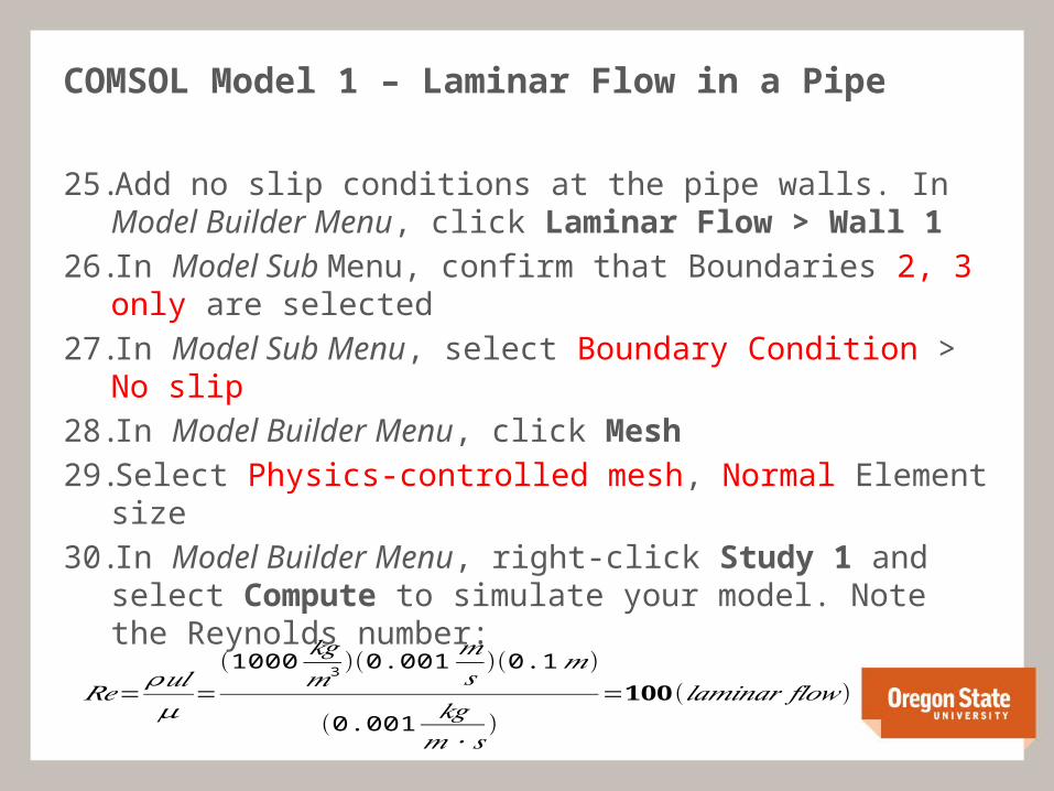
25. Add no slip conditions at the pipe walls. In Model Builder Menu, click Laminar Flow > Wall 1

26. In Model Sub Menu, confirm that Boundaries 2, 3 only are selected

27. In Model Sub Menu, select Boundary Condition > No slip28. In Model Builder Menu, click Mesh29. Select Physics-controlled mesh, Normal Element size30. In Model Builder Menu, right-click Study 1 and select

Compute to simulate your model. Note the Reynolds number:

𝑅𝑒= 𝜌𝑢𝑙𝜇

=(1000

𝑘𝑔𝑚3 )(0.001

𝑚𝑠

)(0.1𝑚)

(0.001 𝑘𝑔𝑚 ∙𝑠

)=𝟏𝟎𝟎 (𝑙𝑎𝑚𝑖𝑛𝑎𝑟 𝑓𝑙𝑜𝑤)

COMSOL Model 1 – Laminar Flow in a Pipe

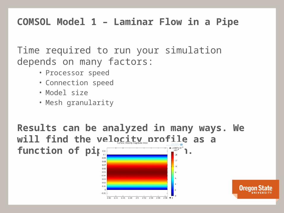
Time required to run your simulation depends on many factors:• Processor speed• Connection speed• Model size• Mesh granularity

Results can be analyzed in many ways. We will find the velocity profile as a function of pipe cross-section.

COMSOL Model 1 – Laminar Flow in a Pipe

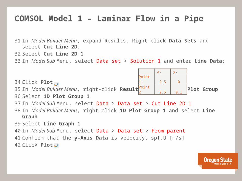
31. In Model Builder Menu, expand Results. Right-click Data Sets and select Cut Line 2D.32. Select Cut Line 2D 133. In Model Sub Menu, select Data set > Solution 1 and enter Line Data:

34. Click Plot 35. In Model Builder Menu, right-click Results and select 1D Plot Group36. Select 1D Plot Group 137. In Model Sub Menu, select Data > Data set > Cut Line 2D 138. In Model Builder Menu, right-click 1D Plot Group 1 and select Line Graph39. Select Line Graph 140. In Model Sub Menu, select Data > Data set > From parent41. Confirm that the y-Axis Data is velocity, spf.U [m/s]42. Click Plot

x: y:Point 1: 2.5 0Point 2: 2.5 0.1

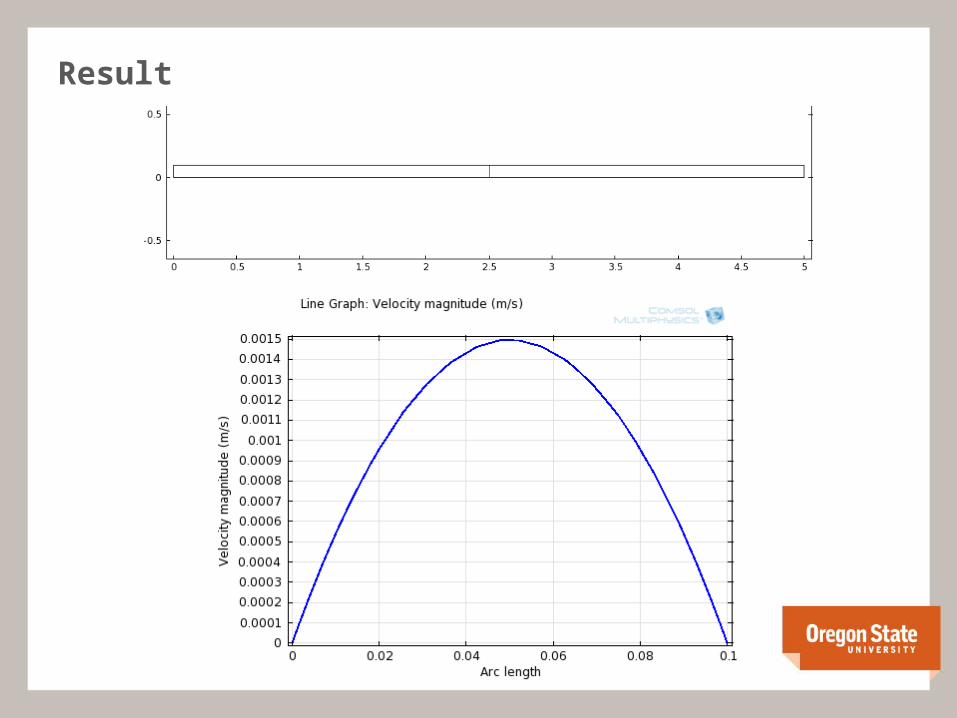
Result

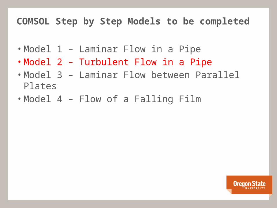
COMSOL Step by Step Models to be completed

• Model 1 – Laminar Flow in a Pipe• Model 2 – Turbulent Flow in a Pipe• Model 3 – Laminar Flow between Parallel Plates• Model 4 – Flow of a Falling Film

COMSOL Model 2 - Turbulent Flow in a Pipe

• Similar to Laminar Flow in a Pipe• Differences:• 3. Turbulent Flow (k-ε)• 19. Enter Uo = 10 m/s• 27. In Model Sub Menu, select Boundary Condition > Wall Functions• Re = 1e6

COMSOL Model 2 - Turbulent Flow in a Pipe

COMSOL Step by Step Models to be completed

• Model 1 – Laminar Flow in a Pipe• Model 2 – Turbulent Flow in a Pipe• Model 3 – Laminar Flow between Parallel Plates• Model 4 – Flow of a Falling Film

COMSOL Model 3 – Laminar Flow between Parallel Plates

• Also similar to Laminar Flow in a Pipe• Differences:• 19. In Model Sub Menu, select Boundary Condition > Pressure, no viscous

stress. Enter po = 0 Pa. Note that both Inlet and Outlet Boundary Conditions are zero pressure. What does this mean?

• After 19:• In Model Builder Menu, right click Laminar Flow and select Wall• Select Wall 2• Define third Boundary Condition by describing the upper plate velocity. On the

Graphic, select the top boundary• In Model Sub Menu, click Add to Selection• In Model Sub Menu, select Boundary Condition > Moving Wall. Enter uw = (0.001, 0)

Pa.• 26. In Model Sub Menu, confirm that Boundary 2 only is selected

COMSOL Model 3 – Laminar Flow between Parallel Plates

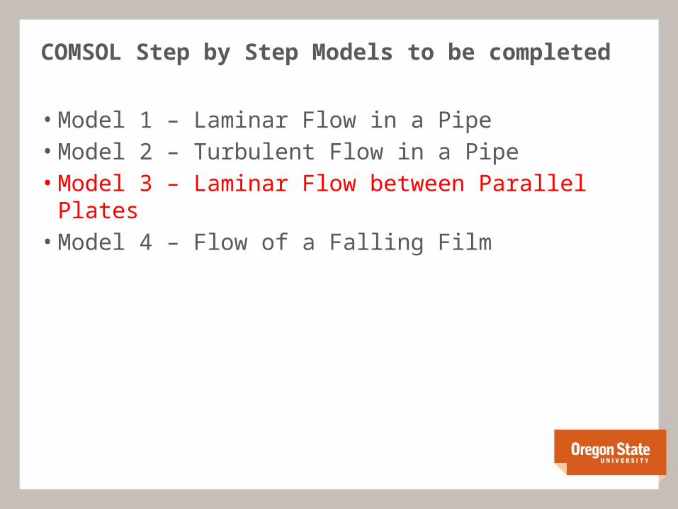
COMSOL Step by Step Models to be completed

• Model 1 – Laminar Flow in a Pipe• Model 2 – Turbulent Flow in a Pipe• Model 3 – Laminar Flow between Parallel Plates• Model 4 – Flow of a Falling Film

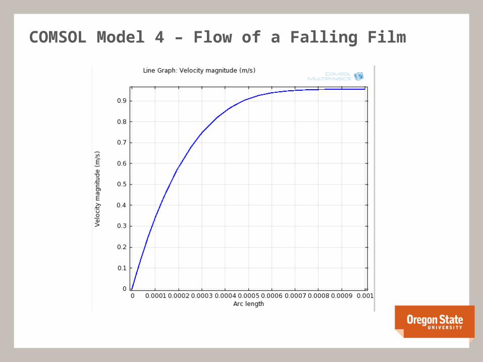
COMSOL Model 4 – Flow of a Falling Film

• Most similar to Laminar Flow between Parallel Plates• Differences:• Make rectangle tall and skinny (W: 0.001 m, H: 0.05 m)• Boundary conditions:• Wall 1 – No Slip• Wall 2 – Outlet, zero pressure• Wall 3 – Inlet, zero velocity• Wall 4 – Open boundary, zero normal stress

• Add Volume Force to Laminar Flow with -9810 N/m3 in the y-direction• Make a horizontal cut line near the bottom of your geometry, to capture

the “fully developed” film flow

COMSOL Model 4 – Flow of a Falling Film