Introduction to Computer Vision

Week 2, Fall 2010 Instructor: Prof. Ko Nishino

Last Week

!  What is Computer Vision !  History of Imaging

"  Camera Obscura

!  Pin-hole Camera !  Thin-lens Law !  Aperture

"  Reciprocity of Aperture-Shutter Speed

!  Defocus, Depth-of-Field !  Distortion

"  Geometric and Radiometric

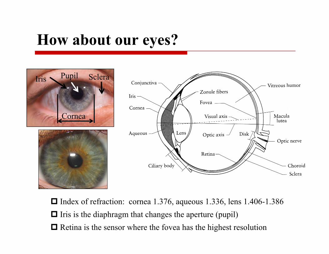
How about our eyes?

#  Index of refraction: cornea 1.376, aqueous 1.336, lens 1.406-1.386 #  Iris is the diaphragm that changes the aperture (pupil) #  Retina is the sensor where the fovea has the highest resolution

Cornea

Sclera Iris Pupil

Accommodation

Changes the focal length of the lens

shorter focal length

Myopia and Hyperopia

(myopia)

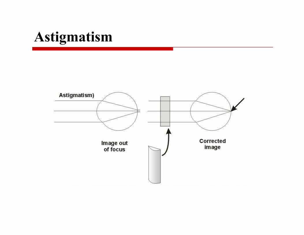
Astigmatism

Image Sensing

Reading: Robot Vision Chapter 2

Human Eye

Rods and Cones

Rods Cones

Achromatic: one type of pigment

Chromatic: three types of pigment

Slow response (long integration time)

Fast response (short integration time)

High amplification High sensitivity

Less amplification Lower absolute sensitivity

Low acuity High acuity

Sensors !  Convert light into electric charge

! CCD (charge coupled device) Higher dynamic range High uniformity Lower noise

! CMOS (complementary metal Oxide semiconductor) Lower voltage

Higher speed Lower system complexity

Sensor Readout

!  CCD

!  CMOS

Images Copyright © 2000 TWI Press, Inc.

Rolling Shutter

!  Read out each row sequentially !  No explicit shutter; controlled sequential exposure !  CMOS !  CCD ! Rolling Shutter !  Introduces distortion for object moving faster than

buffering limit

Rolling Shutter

Figure by Jinwei Gu

Coded Rolling Shutter Photography: Flexible Space-Time Sampling

Jinwei Gu!

Columbia UniversityYasunobu HitomiSony Corporation

Tomoo MitsunagaSony Corporation

Shree NayarColumbia University

Abstract

We propose a novel readout architecture called codedrolling shutter for complementary metal-oxide semiconduc-tor (CMOS) image sensors. Rolling shutter has tradition-

ally been considered as a disadvantage to image quality

since it often introduces skew artifact. In this paper, we

show that by controlling the readout timing and the expo-

sure length for each row, the row-wise exposure discrep-

ancy in rolling shutter can be exploited to flexibly sample

the 3D space-time volume of scene appearance, and can

thus be advantageous for computational photography. The

required controls can be readily implemented in standard

CMOS sensors by altering the logic of the control unit.

We propose several coding schemes and applications:

(1) coded readout allows us to better sample time dimen-

sion for high-speed photography and optical flow based

applications; and (2) row-wise control enables capturing

motion-blur free high dynamic range images from a single

shot. While a prototype chip is currently in development, we

demonstrate the benefits of coded rolling shutter via simu-

lation using images of real scenes.

1. IntroductionCMOS image sensors are rapidly overtaking CCD sen-

sors in a variety of imaging systems, from digital still andvideo cameras to mobile phone cameras to surveillance andweb cameras. In order to maintain high fill-factor and read-out speed, most CMOS image sensors are equipped withcolumn-parallel readout circuits, which simultaneously readall pixels in a row into a line-memory. The readout pro-ceeds row-by-row, sequentially from top to bottom. This iscalled rolling shutter. Rolling shutter has traditionally beenconsidered detrimental to image quality, because pixels indifferent rows are exposed to light at different times, whichoften causes skew and other image artifacts, especially formoving objects [11, 13, 6].

From the perspective of sampling the space-time volumeof a scene, however, we argue that the exposure discrepancyin rolling shutter can actually be exploited using computa-tional photography to achieve new imaging functionalities

!This research was supported in part by Sony Corporation and the Na-tional Science Foundation (IIS-03-25867 and CCF-05-41259).

(a) CMOS image sensor architecture (b) Timing for rolling shutter

Figure 1. The address generator in CMOS image sensors is used to

implement coded rolling shutter with desired row-reset and row-

select patterns for flexible space-time sampling.

and features. In fact, a few recent studies have demonstratedthe use of conventional rolling shutter for kinematics andobject pose estimation [1, 2, 3].

In this paper, we propose a novel readout architecturefor CMOS image sensors called coded rolling shutter. Weshow that by controlling the readout timing and exposurelength for each row of the pixel array, we can flexibly sam-ple the 3D space-time volume of a scene and take pho-tographs that effectively encode temporal scene appearancewithin a single 2D image. These coded images are usefulfor many applications, such as skew compensation, high-speed photography, and high dynamic range imaging.

As shown in Fig. 1, the controls of row-wise readout andexposure can be readily implemented in standard CMOSimage sensors by altering the logic of the address generatorunit without any further hardware modification. For con-ventional rolling shutter, the address generator is simply ashift register which scans all the rows and generates row-reset (RST) and row-select (SEL) signals. For coded rollingshutter, new logics can be implemented to generate the de-sired RST and SEL signals for coded readout and exposure,as shown in Fig. 2. Since the address generator belongs tothe control unit of CMOS image sensors [9, 17], it is easy todesign and implement new logics in the address generatorusing high level tools.

We have begun the process of developing the prototypesensor. We expect to have a fully programmable codedrolling shutter sensor in 18 months. Meanwhile, in this pa-per, we demonstrated coding schemes and their applications

1

Rolling Shutter Distortion

Sensing Brightness

pixel intensity light (photons)

However, incoming light can vary in wavelength

Quantum Efficiency

Pixel intensity:

For monochromatic light with flux :

Sensing Brightness

Incoming light has a spectral distribution

So the pixel intensity becomes

Sensing Color !  Assume we have an image

"  We know the pixel value "  We know our camera parameters

Can we tell the color of the scene? (Can we recover the spectral distribution )

Use a filter Where

then

How do we sense color?

!  Do we have infinite number of filters?

rod

cones

Three filters of different spectral responses

Sensing Color

!  Tristimulus (trichromatic) values Camera’s spectral response functions:

Sensing Color

beam splitter

light

3 CCD Bayer pattern

Foveon X3TM

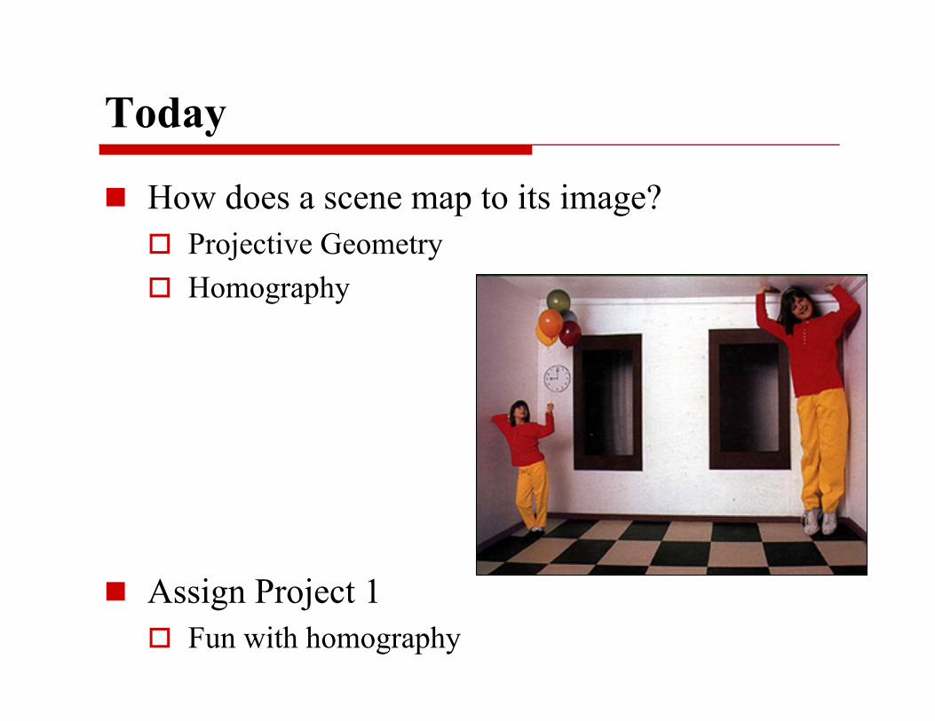
Today

!  How does a scene map to its image? "  Projective Geometry "  Homography

!  Assign Project 1 "  Fun with homography

Camera Models and Projective Geometry

Reading: Zisserman and Mundy book appendix, Simoncelli notes

Modeling Projection

optical axis

center of projection scene point

: effective focal length (will be d from next slide)

Modeling Projection

!  The coordinate system "  We will use the pin-hole model as an approximation "  Put the optical center (Center Of Projection) at the origin "  Put the image plane (Projection Plane) in front of the COP

"  Why? "  The camera looks down the negative z axis

"  we need this if we want right-handed-coordinates

Modeling Projection

!  Perspective Projection "  Compute intersection with PP of ray from (x,y,z) to COP "  Derived using similar triangles

"  We get the projection by throwing out the last coordinate:

Homogeneous Coordinates

!  Is this a linear transformation?

!  Converting from homogeneous coordinates

"  no—division by z is nonlinear

!  Trick: add one more coordinate:

homogeneous image coordinates

homogeneous scene coordinates

Perspective Projection !  Projection is a matrix multiplication using homogeneous

coordinates:

divide by third coordinate

!  This is known as perspective projection "  The matrix is the projection matrix "  Can also formulate as a 4x4 matrix

divide by fourth coordinate

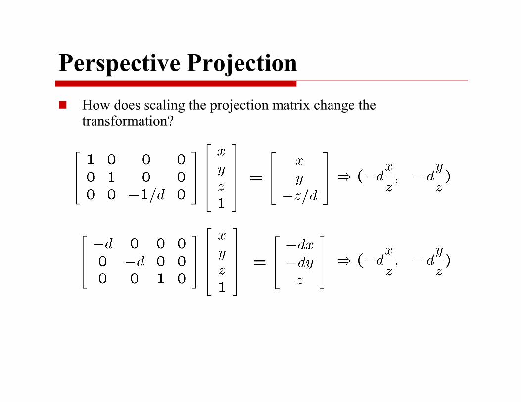
Perspective Projection !  How does scaling the projection matrix change the

transformation?

Orthographic Projection !  Special case of perspective projection

"  Distance from the COP to the PP (effective focal length) is infinite

"  Also called “parallel projection”: (x, y, z) ! (x, y) "  What’s the projection matrix?

Image World

Weak-Perspective Projeciton

!  Scaled orthographic

Affine Projection

!  Also called “paraperspective”

Camera Parameters

!  Projection equation

"  The projection matrix models the cumulative effect of all parameters "  Useful to decompose into a series of operations

!

x =

sxsys

"

#

$ $ $

%

&

' ' '

=

* * * ** * * ** * * *

"

#

$ $ $

%

&

' ' '

XYZ1

"

#

$ $ $ $

%

&

' ' ' '

=(X

!

" =

# fsx 0 x 'c0 # fsy y 'c0 0 1

$

%

& & &

'

(

) ) )

1 0 0 00 1 0 00 0 1 0

$

%

& & &

'

(

) ) )

R3x3 03x101x3 1

$

% & &

'

( ) )

I3x3 T3x1

01x3 1

$

% & &

'

( ) )

projection intrinsics rotation translation

identity matrix

Camera Parameters !  A camera is described by several parameters

"  Translation T of the optical center from the origin of world coords "  Rotation R of the image plane "  focal length f, principle point (x’c, y’c), pixel size (sx, sy) "  blue parameters are called “extrinsics,” red are “intrinsics”

Camera Calibration

!  Goal: estimate the camera parameters "  Version 1: solve for projection matrix

!

x =

wxwyw

"

#

$ $ $

%

&

' ' '

=

* * * ** * * ** * * *

"

#

$ $ $

%

&

' ' '

XYZ1

"

#

$ $ $ $

%

&

' ' ' '

=(X

"  Version 2: solve for camera parameters separately "  intrinsics (focal length, principle point, pixel size) "  extrinsics (rotation angles, translation) "  radial distortion

Estimating the Projection Matrix

!  Place a known object in the scene "  identify correspondence between image and scene "  compute mapping from scene to image

Direct Linear Calibration

Direct Linear Calibration

A 2n ! 12

m 12

0 2n

!  Total least squares "  Since m is only defined up to scale, solve for unit vector "  Minimize

"  Solution: = eigenvector of ATA with smallest eigenvalue "  Works with 6 or more points

Direct Linear Calibration !  Advantage:

"  Very simple to formulate and solve

!  Disadvantages: "  Doesn’t tell you the camera parameters "  Doesn’t model radial distortion "  Hard to impose constraints (e.g., known focal length) "  Doesn’t minimize the right error function

For these reasons, nonlinear methods are preferred •  Define error function E between projected 3D points and image positions

–  E is nonlinear function of intrinsics, extrinsics, radial distortion

•  Minimize E using nonlinear optimization techniques –  e.g., variants of Newton’s method (e.g., Levenberg-Marquart)

Alternative: Multi-Plane Calibration

Images courtesy Jean-Yves Bouguet, Intel Corp.

Advantage •  Only requires a plane •  Don’t have to know positions/orientations •  Good code available online!

–  Intel’s OpenCV library: http://www.intel.com/research/mrl/research/opencv/

–  Matlab version by Jean-Yves Bouget: http://www.vision.caltech.edu/bouguetj/calib_doc/index.html

–  Zhengyou Zhang’s web site: http://research.microsoft.com/~zhang/Calib/