Introduction to Computational Electromagnetics The...
48
Introduction to Computational Electromagnetics The Finite-Element Method Jens Niegemann, Lab for Electromagnetic Fields and Microwave Electronics (IFH), ETH Zürich
Transcript of Introduction to Computational Electromagnetics The...

Introduction to Computational Electromagnetics
The Finite-Element Method
Jens Niegemann, Lab for Electromagnetic Fields and Microwave Electronics (IFH), ETH Zürich

Outline
1) Brief Reminder of Maxwell‘s Equations
2) Introduction to the Finite-Element Method in 1D
3) Practical Computation of the Matrices
4) Implementation of Boundary Conditions/Example
5) Higher-order Elements in 1D
6) Extension to Triangular Meshes (2D)
7) Spurious Modes and Vector Elements
8) Summary
2

BRIEF REMINDER OF MAXWELL‘S EQUATIONS
3

A Reminder of Maxwell’s Equations
In differential form and in time-domain (dim.-less units):
Constitutive Relations (in frequency-domain):
𝝏
𝝏𝒕𝑫 𝐫 , 𝐭 = 𝜵 × 𝑯 𝐫 , 𝐭 − 𝐉 𝐫 , 𝐭 𝜵 ⋅ 𝑫 = 𝟎
𝝏
𝝏𝒕𝑩(𝐫 , 𝐭) = − 𝜵 × 𝐄(𝐫 , 𝐭) 𝜵 ⋅ 𝑩 = 𝟎
4
𝑫 𝒓,𝝎 = 𝝐 𝒓,𝝎 𝑬 𝒓,𝝎 Isotropic, dispersive media
𝑩 𝒓 = 𝑯(𝐫 ) Here: No magnetic response!

A Reminder of Maxwell’s Equations
Transformation to frequency domain: 𝐸 𝑟 , 𝑡 = 𝐸 𝑟 𝑒−𝑖𝜔𝑡
Continuity at material interfaces:
Tangential components continuous
Normal components discontinuous
5
−𝒊𝝎 𝝐 𝐫 𝐄(𝐫 ) = 𝜵 ×𝑯(𝐫 ) − 𝐉 𝐫 , 𝐭 𝜵 ⋅ 𝝐 𝑬 = 𝟎
−𝒊𝝎 𝑯(𝐫 ) = − 𝜵 × 𝐄(𝐫 ) 𝜵 ⋅ 𝑯 = 𝟎
𝝐𝟏 = 𝟏 𝝐𝟐 = 𝟐
𝐸1 𝐸2

The Vector Wave-Equation
Combining the two curl-equations, we find the vector wave-equation
A similar expression can also be derived for 𝐻(𝑟 )
To have a unique solution, we need to provide boundary conditions:
1. Dirichlet Conditions: 𝐄 = 𝐜𝐨𝐧𝐬𝐭 on boundary 𝜕Ω
2. Neumann Conditions: 𝜕
𝜕𝒏 𝐄 = 𝐜𝐨𝐧𝐬𝐭 on boundary 𝜕Ω
3. Mixed/Cauchy Conditions: 𝜕
𝜕𝒏 𝐄 + 𝜸 𝐄 = 𝐜𝐨𝐧𝐬𝐭 on boundary 𝜕Ω
6
𝜵 × 𝜵 × 𝑬 𝐫 − 𝝎𝟐 𝝐 𝐫 𝐄 𝐫 = 𝒊𝝎𝐉 𝐫 , 𝐭

INTRODUCTION TO THE FINITE-ELEMENT
METHOD IN 1D
7

Reduction to the 1D-Wave-Equation
System translationally invariant along (y,z)-axes
Assume bounded domain
Here, simple Dirichlet (PEC) boundary conditions:
𝑬 𝒙𝟎 = 𝑬 𝒙𝑵 = 𝟎
8
𝝏𝒙𝟐 𝑬 𝒙 + 𝝎𝟐𝝐 𝒙 𝑬 𝒙 = −𝒊𝝎𝑱(𝒙)
𝐱 𝐱𝟎 𝐱𝐍
𝛀

Two Approaches to Finite Elements
Two different approaches:
1. Method of weighted residuals/Galerkin‘s Method
2. Variational/Ritz-Approach
In typical cases, both lead to the same discretization!
9

The Method of Weighted Residuals
Assuming we have an approximate solution 𝐸 𝑥 :
𝝏𝒙𝟐 𝑬 𝒙 + 𝝎𝟐𝝐 𝒙 𝑬 𝒙 + 𝒊𝝎𝑱 𝒙 = 𝐑𝐞𝐬 𝒙 ≠ 𝟎
Project the residual onto a set of test functions Ψ𝑖 and
demand that the projection vanishes
𝐑𝐞𝐬 𝒙 ⋅ 𝚿𝐢 𝐱 𝒅𝒙𝛀
= 𝟎
The residual is orthogonal to the function space spanned
by Ψ𝑖
10
Weighting function

The Method of Weighted Residuals
Inserting the expression for 𝐑𝐞𝐬 𝒙 :
𝝏𝒙𝟐 𝑬 𝒙 + 𝝎𝟐𝝐 𝒙 𝑬 𝒙 + 𝒊𝝎𝑱 𝒙 𝚿𝐢 𝐱 𝒅𝒙
𝛀
= 𝟎
Split into separate parts:
𝝏𝒙𝟐 𝑬 𝒙 𝚿𝐢 𝐱 𝒅𝒙
𝛀
+𝝎𝟐 𝝐 𝒙 𝑬 𝒙 𝚿𝐢 𝐱 𝒅𝒙𝛀
= −𝒊𝝎 𝑱 𝒙 𝚿𝐢 𝐱 𝒅𝒙𝛀
Integration by parts: 𝑢′𝑣 𝑑𝑥 =Ω
− 𝑢′𝑣 𝑑𝑥 +Ω
𝑢 𝑣 𝑥0
𝑥𝑁
− 𝝏𝒙 𝑬 𝒙 𝝏𝒙𝚿𝐢 𝒙 𝒅𝒙𝛀
+𝝎𝟐 𝝐 𝒙 𝑬 𝒙 𝚿𝐢 𝐱 𝒅𝒙𝛀
+ 𝝏𝒙 𝑬 𝒙 𝚿𝐢 𝐱𝒙𝟎
𝒙𝑵= 𝑭𝒊
11
=:𝑭𝒊

Choice of the Approximate Solution
Assume an expansion into basis functions 𝚽𝐣 𝐱
𝑬 𝒙 = 𝒆𝒋 𝚽𝐣 𝐱
𝑵
𝒋=𝟎
Insertion into the projections:
𝝎𝟐 𝝐 𝚿𝐢 𝚽𝐣𝒅𝒙𝛀
− 𝝏𝒙𝚿𝒊 𝝏𝒙𝚽𝐣 𝒅𝒙𝛀
+ 𝚿𝐢 𝝏𝒙𝚽𝐣 𝒙𝟎
𝒙𝑵𝒆𝒋
𝑵
𝒋=𝟎
= 𝑭𝒊
Special choice: 𝚽𝐣 𝐱 = 𝚿𝐣 𝐱 (Galerkin‘s Method!)
12

Matrix Form
Leads to symmetric expressions:
𝝎𝟐 𝝐 𝚽𝒊 𝚽𝐣𝒅𝒙𝛀
− 𝝏𝒙𝚽𝒊 𝝏𝒙𝚽𝐣 𝒅𝒙𝛀
+ 𝚽𝐢 𝝏𝒙𝚽𝐣 𝒙𝟎
𝒙𝑵𝒆𝒋
𝑵
𝒋=𝟎
= 𝑭𝒊
Can be written as a matrix-equation:
𝝎𝟐𝑴− 𝑺 + 𝑮 𝒆 = 𝑭
Without source, we have a generalized eigenvalue problem
𝑺 − 𝑮 𝒆 = 𝝎𝟐𝑴 𝒆
13
=:𝑴𝒊𝒋 =: 𝑺𝒊𝒋 =:𝑮𝒊𝒋
Mass-Matrix Stiffness-Matrix

PRACTICAL COMPUTATION OF THE MATRICES
14
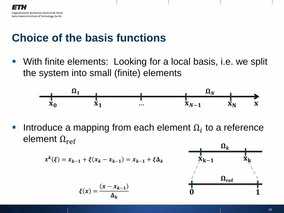
Choice of the basis functions
With finite elements: Looking for a local basis, i.e. we split
the system into small (finite) elements
Introduce a mapping from each element Ω𝑖 to a reference
element Ωref
15
𝐱 𝐱𝟎 𝐱𝐍
𝛀𝟏
𝐱𝟏 𝐱𝑵−𝟏 …
𝛀𝑵
𝐱𝐤−𝟏
𝛀𝒌
𝐱𝐤
𝟎
𝛀𝐫𝐞𝐟
𝟏
𝒙𝒌 𝝃 = 𝒙𝒌−𝟏 + 𝝃 𝒙𝒌 − 𝒙𝒌−𝟏 = 𝒙𝒌−𝟏 + 𝝃𝚫𝒌
𝝃 𝒙 =𝒙 − 𝒙𝒌−𝟏
𝚫𝐤

Considering an individual element
Introducing an interpolatory basis
→ Blackboard
16
𝟎
𝛀𝐫𝐞𝐟
𝟏
𝑬𝟎𝒌 𝑬𝟏
𝒌

Mapping local to global coefficients
Place nodes at interface between elements
Mapping from local dofs to global dofs 𝑬𝟎(𝟏)
𝑬𝟏(𝟏)
𝑬𝟎(𝟐)
𝑬𝟏(𝟐)
𝑬𝟎(𝟑)
𝑬𝟏(𝟑)
𝑬𝟎(𝟒)
𝑬𝟏(𝟒)
=
1 0 0 0 00 1 0 0 00 1 0 0 00 0 1 0 00 0 1 0 00 0 0 1 00 0 0 1 00 0 0 0 1
𝐸0𝐸1𝐸2𝐸3𝐸4
17
𝑬𝟎(𝟏)
𝑬𝟏(𝟏)
𝐱 𝐱𝟎 𝐱𝟒 𝛀𝟏 𝐱𝟏 𝐱𝟑 𝒙𝟐 𝛀𝟒 𝛀𝟐 𝛀𝟑
𝑬𝟎(𝟐)
𝑬𝟏(𝟐)
𝑬𝟎(𝟑)
𝑬𝟏(𝟑)
𝑬𝟎(𝟒)
𝑬𝟏(𝟒)
𝑬𝟎 𝑬𝟏 𝑬𝟐 𝑬𝟑 𝑬𝟒

Construction of the global basis
Expansion:
𝑬 𝒙 = 𝑬𝒋 𝚽𝐣 𝐱
𝑵
𝒋=𝟎
= 𝚽𝟎𝐤 𝑬𝟎
𝒌 +𝚽𝟏𝐤 𝑬𝟏
𝒌
𝑵
𝒌=𝟏
Map to degrees of freedom (dofs):
𝑬 𝒙 = (𝚽𝟎
(𝟏) 𝑬𝟎 +𝚽𝟏
(𝟏) 𝑬𝟏) + (𝚽𝟎
(𝟐)𝑬𝟏 + 𝚽𝟏
(𝟐) 𝑬𝟐) + ⋯+ (𝚽𝟎
(𝐤)𝑬𝒌−𝟏 + 𝚽𝟏
(𝒌) 𝑬𝒌)
Collect global dofs
𝑬 𝒙 = 𝚽𝟎
(𝟏) 𝑬𝟎 + (𝚽𝟏
𝟏+𝚽𝟎
𝟐)𝑬𝟏 +⋯+ (𝚽𝟏
(𝐤−𝟏)+𝚽𝟎
(𝐤))𝑬𝒌−𝟏 + 𝚽𝟏
(𝒌) 𝑬𝒌
18

Construction of the global basis
Expansion:
𝑬 𝒙 = 𝑬𝒋 𝚽𝐣 𝐱
𝑵
𝒋=𝟎
= 𝚽𝟎𝐤 𝑬𝟎
𝒌 +𝚽𝟏𝐤 𝑬𝟏
𝒌
𝑵
𝒌=𝟏
→ Blackboard
19

Final Assembly of the global matrices
With the local matrices at hand, we can easily construct the
global matrices.
General shape: Tri-diagonal because of overlap
𝑴 =
𝑿 𝑿 𝟎 𝟎 𝟎𝑿 𝑿 𝑿 𝟎 𝟎𝟎 𝑿 𝑿 𝑿 𝟎𝟎 𝟎 𝑿 𝑿 𝑿𝟎 𝟎 𝟎 𝑿 𝑿
20

Final Assembly of the global matrices
Iterate over all elements and add local matrices at the right
place:
𝑴 =
𝑴𝟏,𝟏(𝟏) 𝑴𝟏,𝟐
(𝟏)𝟎 𝟎 𝟎
𝑴𝟐,𝟏(𝟏)
𝑴𝟐,𝟐(𝟏)
𝑿 𝟎 𝟎
𝟎 𝑿 𝑿 𝑿 𝟎𝟎 𝟎 𝑿 𝑿 𝑿𝟎 𝟎 𝟎 𝑿 𝑿
21

Final Assembly of the global matrices
Iterate over all elements and add local matrices at the right
place:
𝑴 =
𝑴𝟏,𝟏(𝟏) 𝑴𝟏,𝟐
(𝟏)𝟎 𝟎 𝟎
𝑴𝟐,𝟏(𝟏)
𝑴𝟐,𝟐(𝟏)
+𝑴𝟏,𝟏(𝟐)
𝑴𝟏,𝟐(𝟐)
𝟎 𝟎
𝟎 𝑴𝟐,𝟏(𝟐)
𝑴𝟐,𝟐(𝟐)
𝑿 𝟎
𝟎 𝟎 𝑿 𝑿 𝑿𝟎 𝟎 𝟎 𝑿 𝑿
22

Final Assembly of the global matrices
Iterate over all elements and add local matrices at the right
place:
𝑴 =
𝑴𝟏,𝟏(𝟏) 𝑴𝟏,𝟐
(𝟏)𝟎 𝟎 𝟎
𝑴𝟐,𝟏(𝟏)
𝑴𝟐,𝟐(𝟏)
+𝑴𝟏,𝟏(𝟐)
𝑴𝟏,𝟐(𝟐)
𝟎 𝟎
𝟎 𝑴𝟐,𝟏(𝟐)
𝑴𝟐,𝟐(𝟐)
+𝑴𝟏,𝟏(𝟑)
𝑴𝟏,𝟐(𝟑)
𝟎
𝟎 𝟎 𝑴𝟐,𝟏(𝟑)
𝑴𝟐,𝟐(𝟑)
𝑿
𝟎 𝟎 𝟎 𝑿 𝑿
23

Final Assembly of the global matrices
Iterate over all elements and add local matrices at the right
place:
𝑴 =
𝑴𝟏,𝟏(𝟏) 𝑴𝟏,𝟐
(𝟏)𝟎 𝟎 𝟎
𝑴𝟐,𝟏(𝟏)
𝑴𝟐,𝟐(𝟏)
+𝑴𝟏,𝟏(𝟐)
𝑴𝟏,𝟐(𝟐)
𝟎 𝟎
𝟎 𝑴𝟐,𝟏(𝟐)
𝑴𝟐,𝟐(𝟐)
+𝑴𝟏,𝟏(𝟑)
𝑴𝟏,𝟐(𝟑)
𝟎
𝟎 𝟎 𝑴𝟐,𝟏(𝟑)
𝑴𝟐,𝟐(𝟑)
+𝑴𝟏,𝟏(𝟒)
𝑴𝟏,𝟐(𝟒)
𝟎 𝟎 𝟎 𝑴𝟐,𝟏(𝟒)
𝑴𝟐,𝟐(𝟒)
24

Final Assembly of the global matrices
Stiffness matrix is assembled similarly!
What is still missing is the matrix G = 𝚽𝐢 𝝏𝒙𝚽𝐣 𝒙𝟎
𝒙𝑵
𝑮 =
𝑮𝟎,𝟎 𝑮𝟎,𝟏 𝟎 𝟎 𝟎
𝟎 𝟎 𝟎 𝟎 𝟎𝟎 𝟎 𝟎 𝟎 𝟎𝟎 𝟎 𝟎 𝟎 𝟎𝟎 𝟎 𝟎 𝑮𝑵,𝑵−𝟏 𝑮𝑵,𝑵
Plays a certain role for some boundary conditions!
25

IMPLEMENTATION OF BOUNDARY CONDITIONS
26

Dirichlet Boundary Conditions
Assuming PEC boundary conditions: 𝐸 𝑥0 = 𝐸 𝑥𝑁 = 𝑐
𝑿 𝑿 𝟎 𝟎 𝟎𝑿 𝑿 𝑿 𝟎 𝟎𝟎 𝑿 𝑿 𝑿 𝟎𝟎 𝟎 𝑿 𝑿 𝑿𝟎 𝟎 𝟎 𝑿 𝑿
𝑬𝟎𝑬𝟏𝑬𝟐𝑬𝟑𝑬𝟒
=
𝑭𝟎𝑭𝟏𝑭𝟐𝑭𝟑𝑭𝟒
To enforce boundary conditions, we replace the r.h.s. with
the fixed value and modify the equation
27

Dirichlet Boundary Conditions
Assuming PEC boundary conditions: 𝐸 𝑥0 = 𝐸 𝑥𝑁 = 𝑐
𝟏 𝟎 𝟎 𝟎 𝟎𝑨 𝑿 𝑿 𝟎 𝟎𝟎 𝑿 𝑿 𝑿 𝟎𝟎 𝟎 𝑿 𝑿 𝑩𝟎 𝟎 𝟎 𝟎 𝟏
𝑬𝟎𝑬𝟏𝑬𝟐𝑬𝟑𝑬𝟒
=
𝒄𝑭𝟏𝑭𝟐𝑭𝟑𝒄
Matrix is no longer symetric, but can be fixed!
28

Dirichlet Boundary Conditions
Assuming PEC boundary conditions: 𝐸 𝑥0 = 𝐸 𝑥𝑁 = 𝑐
𝑿 𝑿 𝟎𝑿 𝑿 𝑿𝟎 𝑿 𝑿
𝑬𝟏𝑬𝟐𝑬𝟑
=𝑭𝟏 − 𝒄𝑨
𝑭𝟐𝑭𝟑 − 𝒄𝑩
Matrix is symetric again!
The fixed unknowns can be removed from the system. Can
save significant number of dofs in 2D and 3D
29

HIGHER-ORDER ELEMENTS IN 1D
30

Considering an individual element
Instead of linear interpolation, we can also use quadratic
On the reference element, we now need three nodes!
→ Blackboard
31
𝑬𝟎(𝟏)
𝑬𝟐(𝟏)
𝐱 𝐱𝟎 𝐱𝟒 𝛀𝟏 𝐱𝟏 𝐱𝟑 𝒙𝟐 𝛀𝟒 𝛀𝟐 𝛀𝟑
𝑬𝟎 𝑬𝟏 𝑬𝟐 𝑬𝟑 𝑬𝟒
𝟎 𝛀𝐫𝐞𝐟 𝟏
𝑬𝟎𝒌 𝑬𝟐
𝒌 𝑬𝟏𝒌
𝑬𝟏(𝟏)

Plot of the basis functions
32

Comparison of Convergence
33
Convergence: 𝐸 − 𝐸 ≤ 𝑐 ℎ𝑝+1

EXTENSION TO TRIANGULAR MESHES (2D)
34

TM-Polarization
In TM-Polarization, we can describe the entire dynamics
via the 𝐸𝑧(𝑥, 𝑦)-field
Galerkin-Procedure analogous to 1D
35
𝝏𝒙𝟐 𝑬 𝒙, 𝒚 + 𝝏𝒚
𝟐 𝑬 𝒙, 𝒚 + 𝝎𝟐𝝐 𝒙, 𝒚 𝑬 𝒙, 𝒚 = −𝒊𝝎𝑱(𝒙, 𝒚)
→ Blackboard

Elements in 2D
Typically, one uses triangular or quadrilateral elements
First step: Mesh generation
Similarly to 1d-case, we need
1. Mapping to reference element
2. Local matrices
3. Mapping global to local nodes
→ Blackboard
36

Elements in 2D
Assembly is almost identical to the 1D-Case, but matrix not
tri-diagonal!
Matrices are much larger now: Use specialized sparse
matrix solvers or iterative methods!
Convergence properies as before: 𝐸 − 𝐸 ≤ 𝑐 ℎ𝑝+1
It is also possible to use curved elements!
37

SPURIOUS MODES AND VECTOR ELEMENTS
38

Vectorial Problems
In 3D, we can no longer reduce the problem to a scalar
field:
Idea: Repeat all steps as before, but use basis-functions
for each component independently:
Φ𝑖 ∈Φ𝑖
00
,0Φ𝑖
0,
00Φ𝑖
Freitag, 16. März 2012 39
𝜵 × 𝜵 × 𝑬 𝐫 − 𝝎𝟐 𝝐 𝐫 𝐄 𝐫 = 𝒊𝝎𝐉 𝐫 , 𝐭

Problems with this approach
Does not work very well: In eigenvalue problems one find
spurious modes.
The physical reason is, that we are not solving the full
Maxwell‘s equations, but only the curl-equations.
By taking the divergence of the wave-equation
we find:
Freitag, 16. März 2012 40
𝜵 × 𝜵 × 𝑬 𝐫 = 𝝎𝟐 𝝐 𝐫 𝐄 𝐫
𝝎𝟐 𝛁 𝝐 𝐫 𝐄 𝐫 = 𝟎
Reasons for the Spurious Modes
For 𝜔 ≠ 0, we have the divergence condition build in!
But, for 𝜔 = 0, we will also find solutions, which are
unphysical!
The null-space is of infinite size, since every function
is a solution for 𝜔 = 0.
Freitag, 16. März 2012 41
𝑬 𝒓 = 𝛁𝚽

Poor Numerical Approximation of the Null-Space
The large null-space in itself is not a problem!
Due to poor numerical approximation, we find spurious
non-zero eigenvalues inbetween the correct values
Mathematically, the underlying problem is related to the
discontinuity of the fields at interfaces!
With our current basis functions, we enforce continuity
since we share field-values on nodes or edges!
Freitag, 16. März 2012 42

A simple example
Physical Modes of a rectangular cavity
Freitag, 16. März 2012 43

A simple example
Modes in the null-space of a rectangular cavity
Freitag, 16. März 2012 44

Solution
The common solution: Use more suitable basis functions
Here, Whitney elements (vector elements):
Freitag, 16. März 2012 45
→ Blackboard

Plot of the First-Order Whitney Elements
Freitag, 16. März 2012 46 Departement/Institut/Gruppe

SUMMARY
47

Summary
Finite-Element Method (FEM) is a very powerful and highly
accurate volume method
It leads to linear systems of equations with very sparse
matrices which are easily assembled
For vectorial problems, one should work approp. elements
There is a large variety of commerical (Comsol, JCMWave,
HFSS, Microwave Studio) and open-source frameworks
(Deal.II, FreeFem, Dune, …) available!
48