
Introduction to business cycle theory -...
47
Introduction to business cycle theory ● Following the works of Lucas on rational expectations a new strand of the literature on Macroeconomics has emerged at the start of the 80s (New Classical School) → the so-called RBC approach ● Short-run fluctuations are thought of as corresponding to the result of the optimal's response of the economy subject to productivity shocks. ● Beyond the theoretical approach, it is the methodolical innovation which is now still popular among macroeconomists → DGSE models
Transcript of Introduction to business cycle theory -...
Introduction to business cycle theory
● Following the works of Lucas on rational expectations a new strand of the literature on Macroeconomics has emerged at the start of the 80s (New Classical School)
→ the so-called RBC approach● Short-run fluctuations are thought of as corresponding
to the result of the optimal's response of the economy subject to productivity shocks.
● Beyond the theoretical approach, it is the methodolical innovation which is now still popular among macroeconomists
→ DGSE models

The RBC approach has been initiated by Kydland and E. Prescott (1982, Nobel Prize in 2005).→ In the line of the Lucas critique to Keynesianism: Building a model with explicit micro-foundations taking part in the general equilibrium analysis: market clearing, no monetary factors, at odds with keynesian tradition.
→ No rationale for macroeconomic management = the optimal growth model with short-run fluctuations induced by productivity shocks (stochastic neoclassical growth model in the line of Solow (1956) and Cass-Koopmans (1965)) – see also Chapter 5 on growth theory.
The methodology:→ building a successful (relative to data) business cycle model: imposing a new method based on calibration to evaluate the performance of business cycle models relative to a new definition of the business cycle facts. Quantitative Approach.
→ This methology has been criticized but is now extensively used in macroeconomics today, even by proponents of stabilization interventions. → used in all areas of economics→ even used in frameworks that invoke market failures so that government interventions are desirable.
● The main issues→ what are the factor behind business cycles (real or nominal)?→ are the fluctuations optimal or the « proof » that the economic system is characterized by inefficiencies?→ is there a need to stabilize (welfare costs of the business cycles)?→ what are the policies likely to stabilize the business cycle?

Plan of the talk
1. The RBC approach2. Solving the model3. Quantitative discussion

1. The RBC Model
We consider a Neoclassical growth model in the line of Cass [1965] More specifically:→ consumption > permanent income component
→ investment > capital accumulation→ labor market clears→ productivity shocks to initiate the business cycle
See Plosser [1989], Journal of Economic Perspectives.

Assumptions● Perfectly competitive economy● Optimal growth model + aggregate shocks to
productivity + labor decisions● 2 types of agents: one representative household and
one representative firm● Pareto optimal economy (equilibrium allocation =
planner's solution)→ The planner's allocation can be decentralized by considering a competitive equilibrium where households own the firms
Preferences
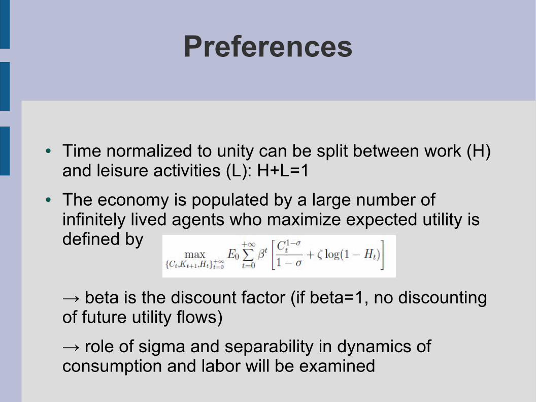
● Time normalized to unity can be split between work (H) and leisure activities (L): H+L=1
● The economy is populated by a large number of infinitely lived agents who maximize expected utility is defined by
→ beta is the discount factor (if beta=1, no discounting of future utility flows)
→ role of sigma and separability in dynamics of consumption and labor will be examined

Technology
● We consider a Cobb-Douglas production function that incorporates secular improvement in factor productivity
where A refers to random shock and X is the deterministic component of productivity: →
● AR(1) process for the random technology

National income accounts● The output can be used for consumption or investment
● The stock of capital evolves according to the level of investment and the depreciation rate of existing capital:
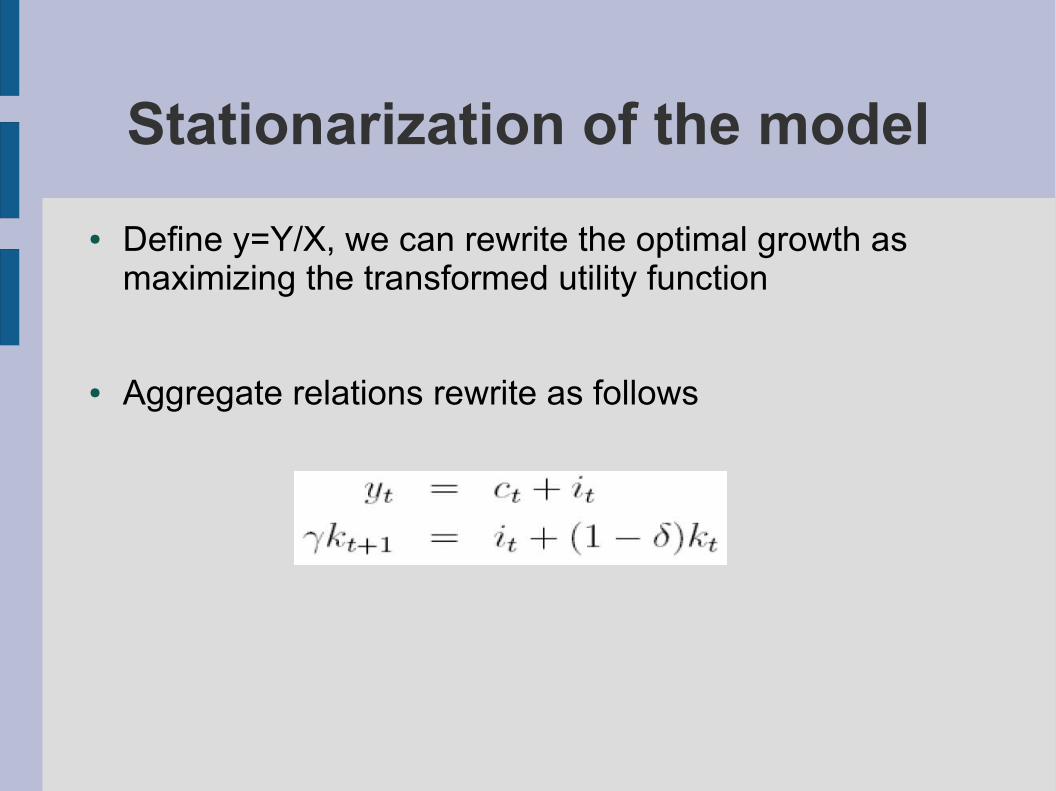
Stationarization of the model● Define y=Y/X, we can rewrite the optimal growth as
maximizing the transformed utility function
● Aggregate relations rewrite as follows

Private decisions of the household
● The household maximizes its expected life-time utility (current + expected) conditional to current capital stock and technology→ he chooses a consumption/saving stream and a labor supply by expecting the future value of the productivity level
st. the BC where r is the rental price of capital and w the wage rate who both depend on technology and capital stock levels (profits are equal to zero)
and transversality condition
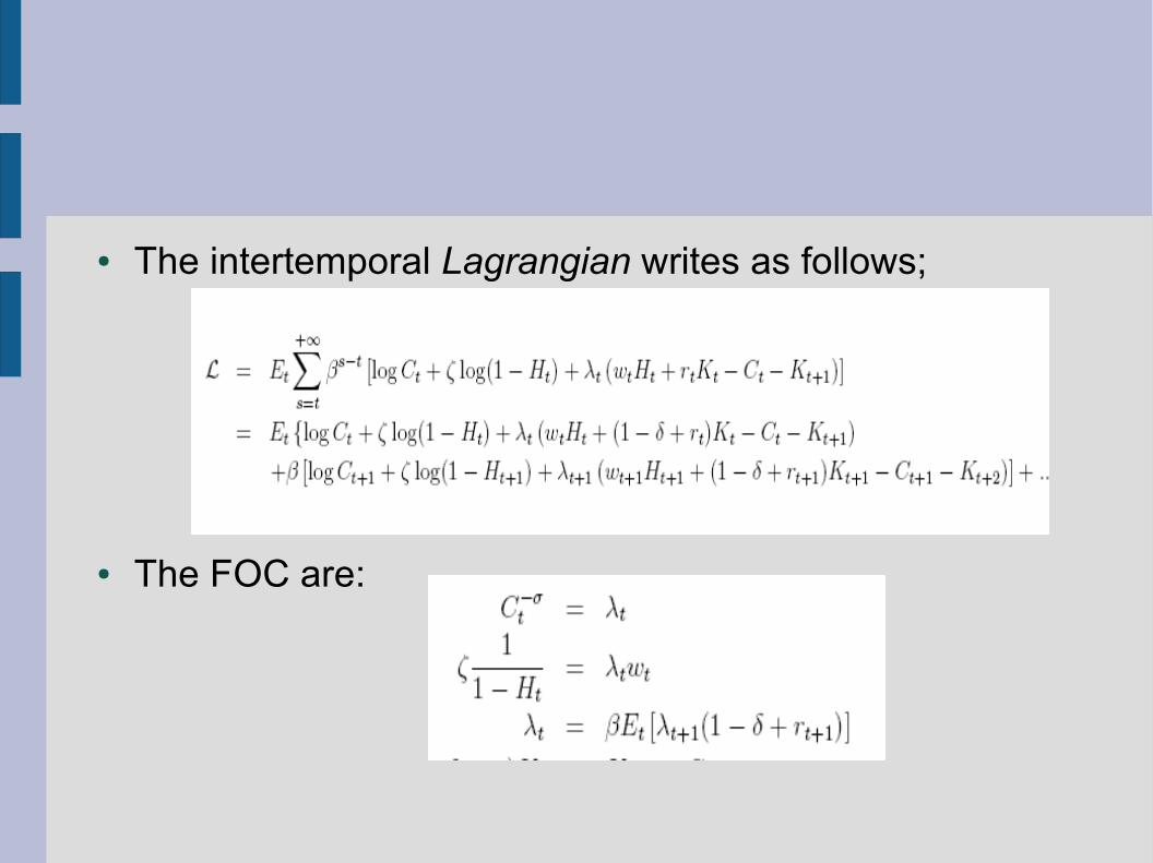
● The intertemporal Lagrangian writes as follows;
● The FOC are:

● Comments of the FOC:→ First condition: The present marginal utility of consumption is equal to the expected and discounted marginal value (in terms of utility) of capital.
→ Second condition : The marginal rate of substitution between consumption and leisure is equal to the real wage. → Third condition: the expected and discounted marginal value of capital is given on the optimal path by the interest factor evaluated in terms of the marginal utility of consumption tomorrow

→ The third and the first conditions determine together the so-called stochastic Euler (or Keynes-Ramsey) condition which relies the marginal rate of substitution between current and future consumptions to the rental rate:
→ the consumption is more increasing than interest rate (time preferences) is high (low)
→ if sigma is high (=low intertemporal substitution) the dynamics of consumption is less sensitive to variations in expected interest rate

Firms' behavior● The firms (own by the household) solve a static
problem by choosing labor demand and capital to maximize at each date profit flows:
● FOC
● Given constant return to scales, straightforward to see that profits will always be equal to zero.

The impact of productivity disturbances: preliminary discussion

2.1 Solving the model : Analytical case
● If we consider complete capital depreciation ( )and log-utility function ( ),we can derive a closed-form solution of the model
● The intertemporal general equilibrium is given by

● This yields to the following deflated equilibrium:

● Solution:
Notice that
From Euler equation, one gets:
Denote
→

● The solution of the canonical RBC model is then given by:
● Total hours are constant (→ empirical puzzle)

2.2 Solving the model :the general case
● In general no analytical solution exist for the non-linear system of stochastic finite difference equations under rational expectations→ need to rely on approximation methods
→ log-linearize the model around the steady-state→ solve the linearized model using standard techniques
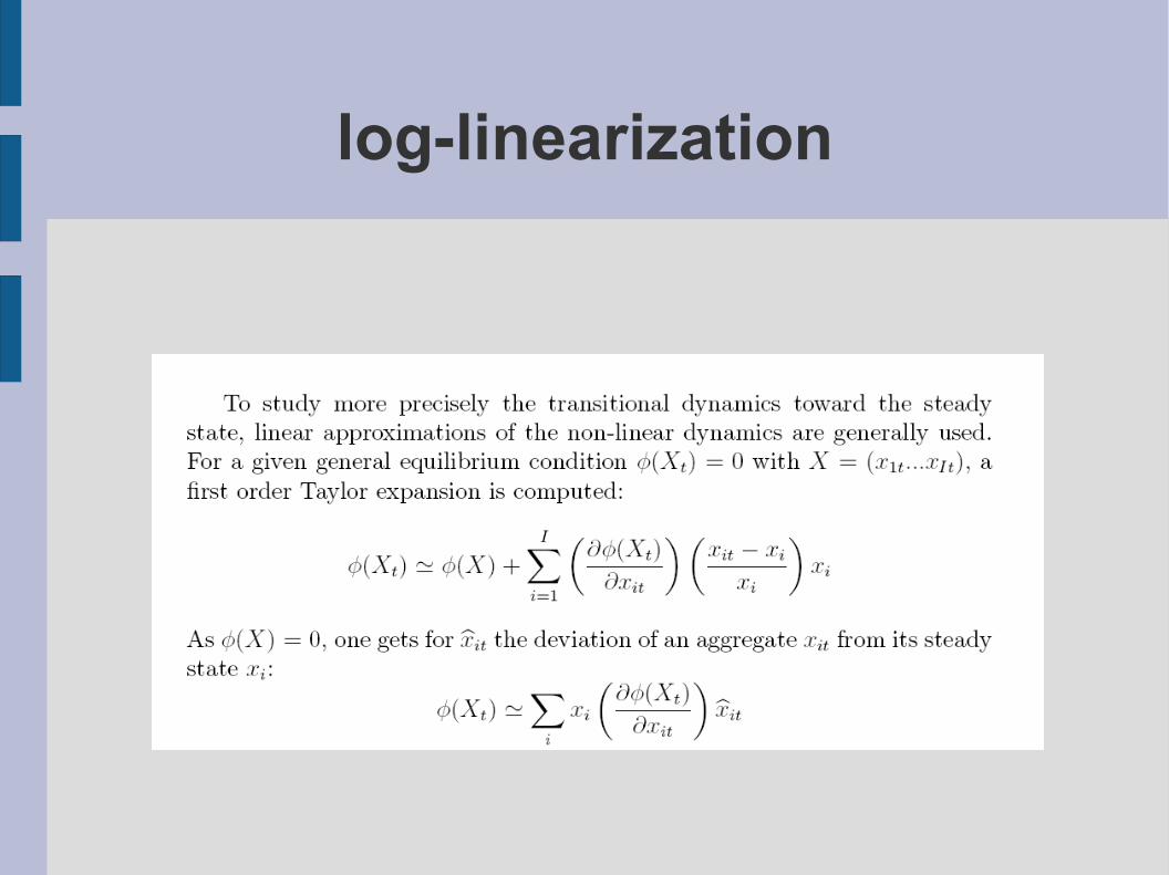
log-linearization
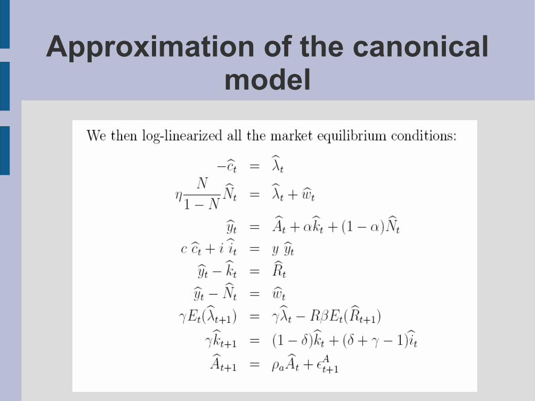
Approximation of the canonical model
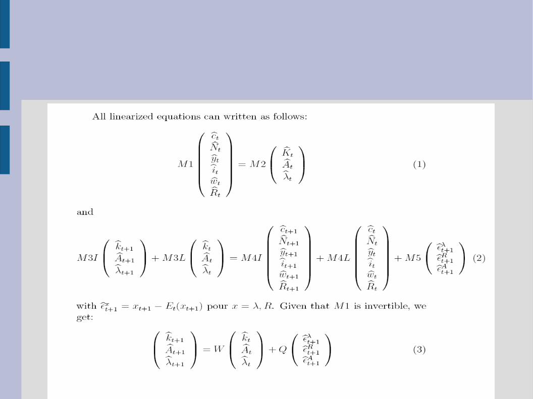


Saddle-path equilibrium
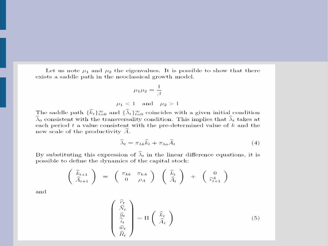

● This model solution can then be used to simulate the model → calibration procedure→ compare model predictions and characteristics of historical data→ is there any empirical puzzles?→ no policy recommandation at this stage (fluctuations are consistent with the response of a Pareto-efficient economy to productivity disturbances)
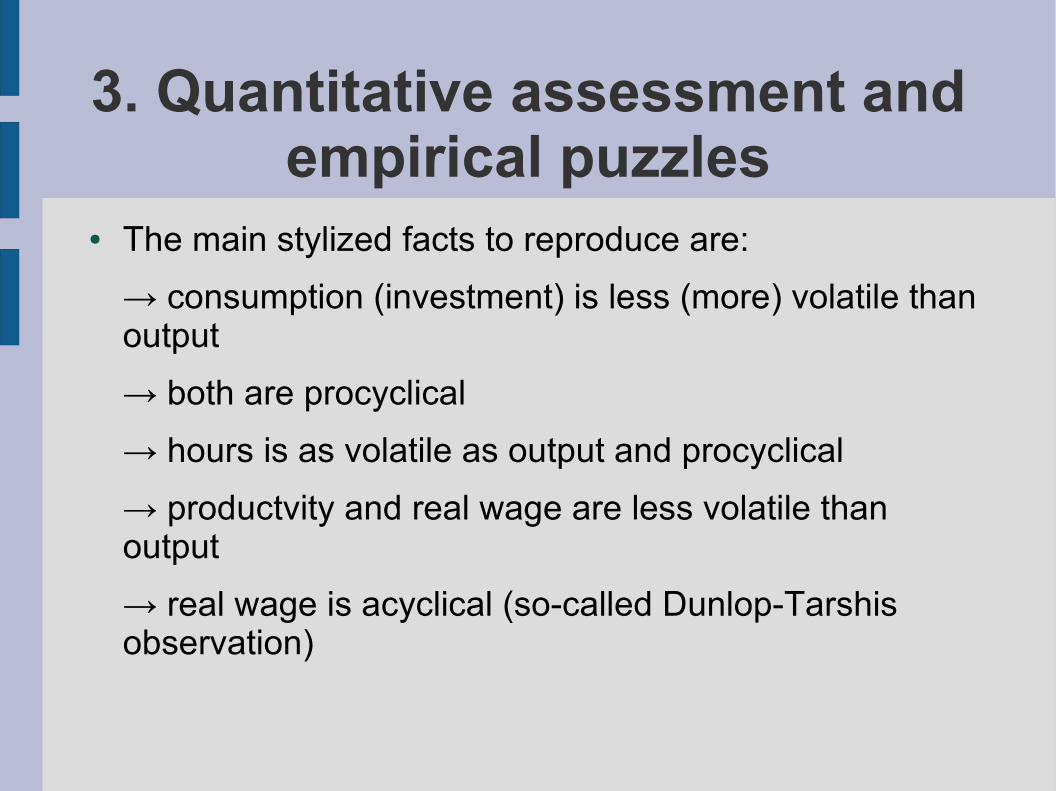
3. Quantitative assessment and empirical puzzles
● The main stylized facts to reproduce are:→ consumption (investment) is less (more) volatile than output→ both are procyclical→ hours is as volatile as output and procyclical
→ productvity and real wage are less volatile than output
→ real wage is acyclical (so-called Dunlop-Tarshis observation)
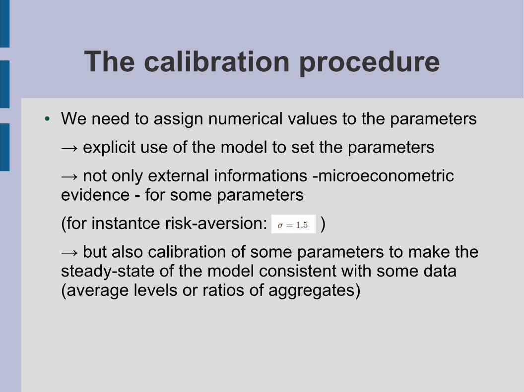
The calibration procedure● We need to assign numerical values to the parameters
→ explicit use of the model to set the parameters
→ not only external informations -microeconometric evidence - for some parameters (for instantce risk-aversion: )
→ but also calibration of some parameters to make the steady-state of the model consistent with some data (average levels or ratios of aggregates)

Calibration on US data● We have to set● We can use observed data for
and growth rate per quarter→ In the data ; use capital accumulation to get
→ In the data and the model implies
→ In the data ; using Euler equation we get >→ In the data H=.31, and this implies
The role of capital dynamics● In a preliminary step we want to examine whether
capital dynamics can account for Business Cycle→ consider perfect foresights dynamics with fixed vs. variable labor cases
→ consider that capital is 1% below its steady-state value
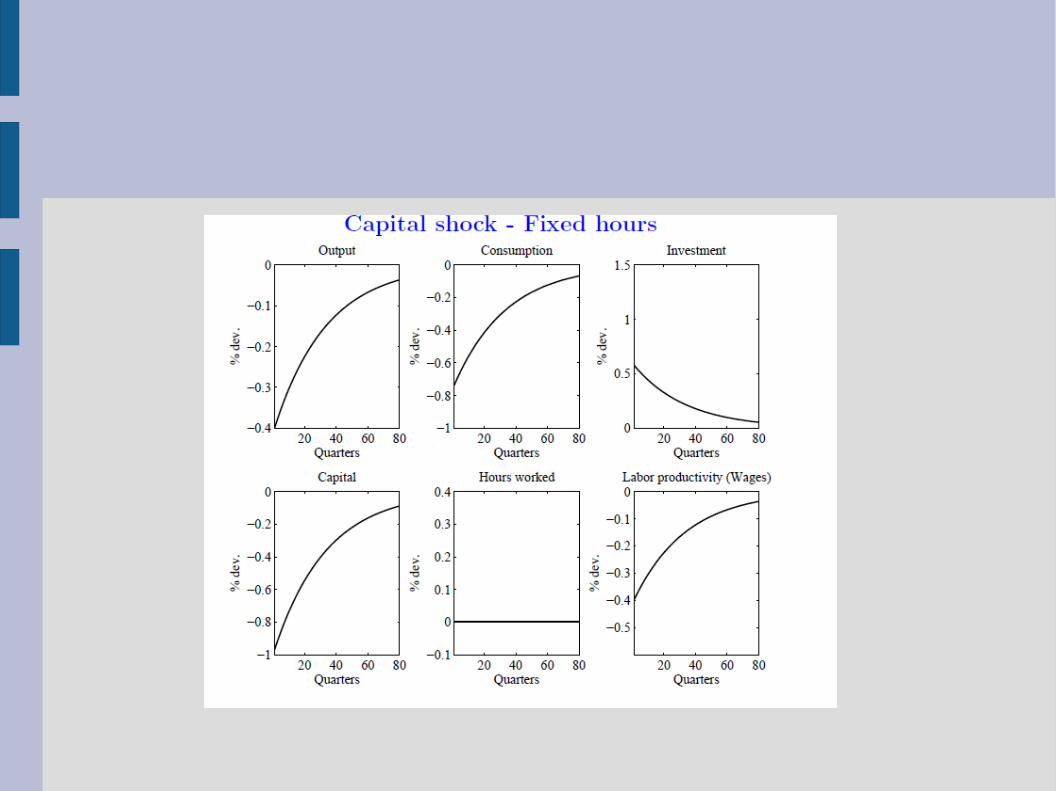
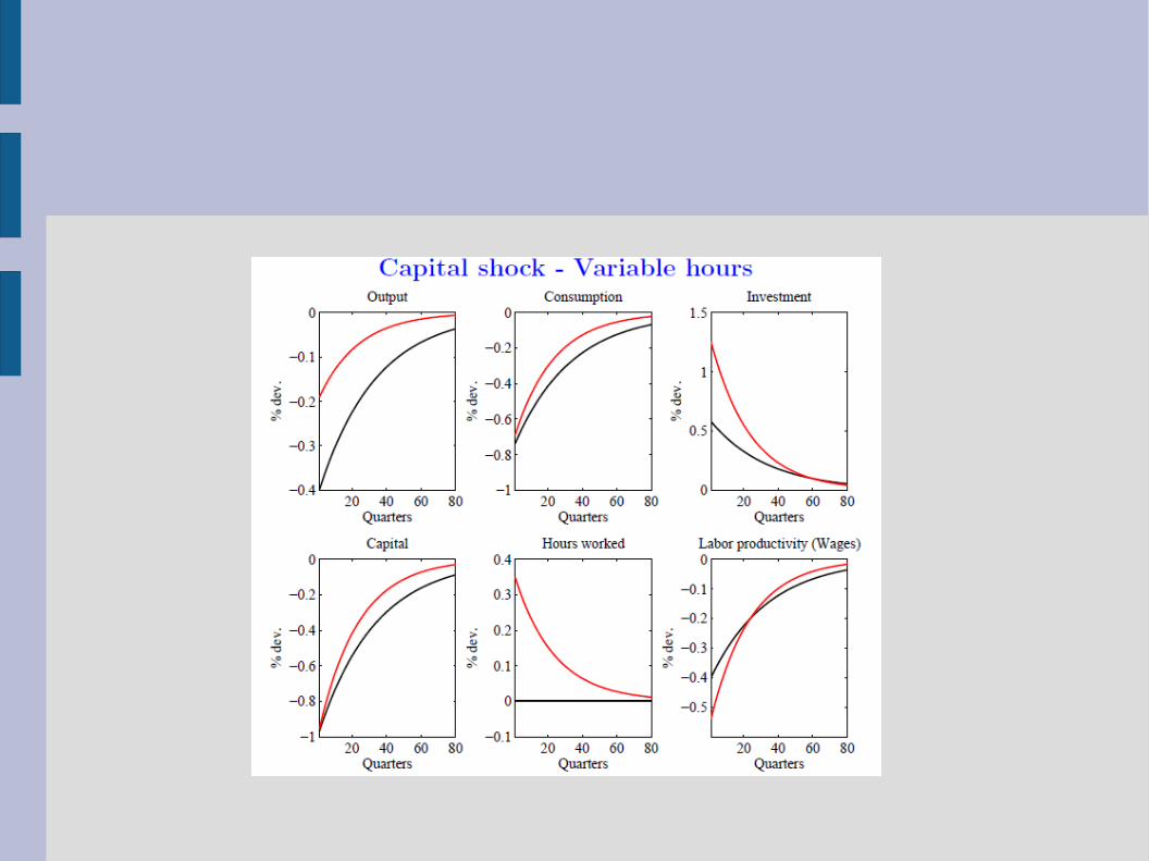

● Capital dynamics cannot be the story for the business cycle→ Solow (1957) already showed that capital accumulation only account for 1/8th of output growth→ Technical progress is the engine of growth
● Transitional dynamics of consumption and investment are negatively correlated in opposition to data
● RBC literature introduces technological shocks

The role of technological shocks
● To calibrate those shocks, use the Solow Residual● We assumed that ● Use historical series for k and y, and then estimate
→ this implies and

Model simulations with estimated shocks
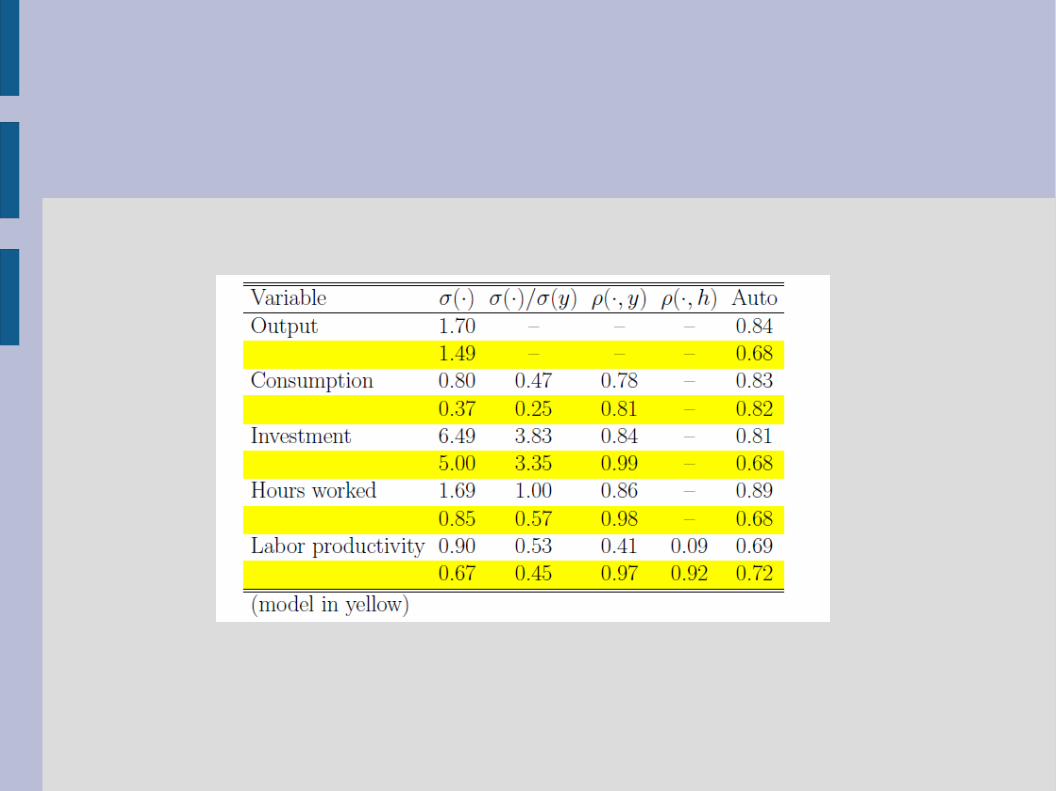
The empirical puzzles● Quite good fit of consumption, investment and output
→ correct ranking of volatilities and correlations
→ the RBC model captures the general pattern of comovements in the data
● But, relative volatility of hours workers is twice lower, and procyclicality of productivity (and real wage) is substantially greater than in the data→ the understanding of the labor market functionning is not good

Other criticisms● The research on RBC becomes so successful because
it proposes a coherent framework/methodology to analyze fluctuations
● Counterfactual predictions● Theoretical concern: productivity shocks are the main
perturbation of optimal fluctuations● Problem of the measure of technological shocks
→ Technological shocks account for 70% of output volatility but little evidence of large supply shocks + recessions have to be explained→ Need of very persistent shocks ↔ the model possesses weak propagation mechanisms


![Untitled-1 [photopedia.info] · 2018-06-15 · 12*GRlECHENLAND 105 12kGRIECHENLANbJ CLANDSCHAFTEN ) 10 Christa Bauer 1 Acheron 2 Dadia 3 Lasithi-Hochebene 4 Mani 5 Methana 6 Pilion](https://static.fdocuments.us/doc/165x107/5e6088f720d710728e33a61b/untitled-1-2018-06-15-12grlechenland-105-12kgriechenlanbj-clandschaften-.jpg)