Introduction to belief functions - Gipsa-lab · A belief function may be viewed both as...

BasicsSelected advanced topics

Introduction to belief functions

Thierry Denœux1

1Université de Technologie de CompiègneHEUDIASYC (UMR CNRS 6599)

http://www.hds.utc.fr/˜tdenoeux

Spring School BFTA 2011Autrans, April 4-8, 2011

Thierry Denœux Introduction to belief functions 1/ 70


Contents of this lecture

1 Context, position of belief functions with respect toclassical theories of uncertainty.

2 Fundamental concepts: belief, plausibility, commonality,Conditioning, basic combination rules.

3 Some more advanced concepts: least commitmentprinciple, cautious rule, multidimensional belief functions.



Uncertain reasoning

In science and engineering we always need to reason withpartial knowledge and uncertain information (from sensors,experts, models, etc.).Different kinds of uncertainty:

Aleatory uncertainty induced by the variability of entities inpopulations and outcomes of random (repeatable)experiments. Example: drawing a ball from an urn. Cannotbe reduced;Epistemic uncertainty, due to lack of knowledge. Example:inability to distinguish the color of a ball because of colorblindness. Can be reduced.

Classical frameworks for reasoning with uncertainty:1 Probability theory;2 Set-membership approach.



Probability theoryInterpretations

Probability theory can be used to represent:Aleatory uncertainty: probabilities are considered asobjective quantities and interpreted as frequencies or limitsof frequencies;Epistemic uncertainty: probabilities are subjective,interpreted as degrees of belief.

Main objections against the use of probability theory as amodel epistemic uncertainty (Bayesian model):

Inability to represent ignorance;Not a plausible model of how people make decisions basedon weak information.



Inability to represent ignoranceThe wine/water paradox

Principle of Indifference (PI): in the absence of informationabout some quantity X , we should assign equal probabilityto any possible value of X .The wine/water paradox:There is a certain quantity of liquid. All that we know aboutthe liquid is that it is composed entirely of wine and water,and the ratio of wine to water is between 1/3 and 3. Whatis the probability that the ratio of wine to water is less than

or equal to 2?



Inability to represent ignoranceThe wine/water paradox (continued)

Let X denote the ratio of wine to water. All we know is thatX ∈ [1/3,3]. According to the PI, X ∼ U[1/3,3].Consequently:

P(X ≤ 2) = (2− 1/3)/(3− 1/3) = 5/8.

Now, let Y = 1/X denote the ratio of water to wine.Similarly, we only know that Y ∈ [1/3,3]. According to thePI, Y ∼ U[1/3,3]. Consequently:

P(X ≤ 2) = P(Y ≥ 1/2)

= (3− 1/2)/(3− 1/3) = 15/16.



Decision makingEllsberg’s paradox

Suppose you have an urn containing 30 red balls and 60balls, either black or yellow. You are given a choicebetween two gambles:

A: You receive 100 euros if you draw a red ball;B: You receive 100 euros if you draw a black ball.

Also, you are given a choice between these two gambles(about a different draw from the same urn):

C: You receive 100 euros if you draw a red or yellow ball;D: You receive 100 euros if you draw a black or yellow ball.

Most people strictly prefer A to B, henceP(red) > P(black), but they strictly prefer D to C, hence

P(black) + P(yellow) > P(red) + P(yellow)

⇒ P(black) > P(red).



Set-membership approach

Partial knowledge about some variable X is described by aset of possible values E (constraint).Example:

Consider a system described by the equation

y = f (x1, . . . , xn; θ)

where y is the output, x1, . . . , xn are the inputs and θ is aparameter.Knowing that xi ∈ [x i , x i ], i = 1, . . . ,n and θ ∈ [θ, θ], find aset X surely containing x .

Advantage: computationally simpler than the probabilisticapproach in many cases (interval analysis).Drawback: no way to express doubt, conservativeapproach.



Theory of belief functions

Alternative theories of uncertainty:Possibility theory (Zadeh, 1978; Dubois and Prade1980’s-1990’s);Imprecise probability theory (Walley, 1990’s);Theory of belief functions (Dempster-Shafer theory,Evidence theory, Transferable Belief Model) (Dempster,1968; Shafer, 1976; Smets 1980’s-1990’s).

The theory of belief functions extends both theSet-membership approach and Probability Theory:

A belief function may be viewed both as a generalized setand as a non additive measure.The theory includes extensions of probabilistic notions(conditioning, marginalization) and set-theoretic notions(intersection, union, inclusion, etc.)



Outline

1 BasicsBelief representationInformation fusionDecision making

2 Selected advanced topicsInformational orderingsCautious ruleMultidimensional belief functions



Belief representationInformation fusionDecision making

Outline






Mass functionDefinition

Let X be a variable taking values in a finite set Ω (frame ofdiscernment).Mass function: m : 2Ω → [0,1] such that∑

A⊆Ω

m(A) = 1.

Every A of Ω such that m(A) > 0 is a focal set of m.m is said to be normalized if m(∅) = 0. This condition maybe required or not.




Murder example

A murder has been committed. There are three suspects:Ω = Peter , John,Mary.A witness saw the murderer going away in the dark, and hecan only assert that it was man. How, we know that thewitness is drunk 20 % of the time.This piece of evidence can be represented by

m(Peter , John) = 0.8,

m(Ω) = 0.2

The mass 0.2 is not committed to Mary, because thetestimony does not accuse Mary at all!




Mass functionMulti-valued mapping interpretation

(Θ, P) Ω

Γdrunk

not drunk

Peter

JohnMary

A mass function m on Ω may be viewed as arising fromA set Θ = θ1, . . . , θr of interpretations;A probability measure P on Θ;A multi-valued mapping Γ : Θ→ 2Ω.

Meaning: under interpretation θi , the evidence tells us thatX ∈ Γ(θi), and nothing more. The probability P(θi) istransferred to Ai = Γ(θi).m(A) is the probability of knowing only that X ∈ A, giventhe available evidence.




Mass functionsSpecial cases

Only one focal set:

m(A) = 1 for some A ⊆ Ω

→ categorical (logical) mass function (∼ set). Specialcase: A = Ω, vacuous mass function, represents totalignorance.All focal sets are singletons:

m(A) > 0⇒ |A| = 1

→ Bayesian mass function (∼ probability mass function).A mass function can thus be seen as

a generalized set;a generalized probability distribution.




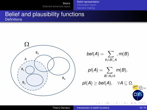
Belief and plausibility functionsDefinitions

Ω

A

B1

B2

B3

B4

bel(A) =∑∅6=B⊆A

,m(B)

pl(A) =∑

B∩A6=∅

m(B),

pl(A) ≥ bel(A), ∀A ⊆ Ω.




Belief and plausibility functionsInterpretation and special cases

Interpretations:bel(A) = degree to which the evidence supports A.pl(A) = upper bound on the degree of support that could beassigned to A if more specific information became available.

Special case: if m is Bayesian, bel = pl (probabilitymeasure).




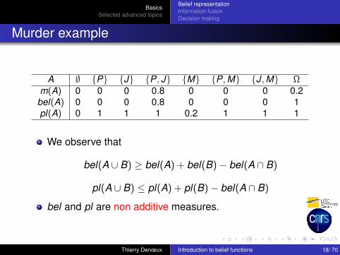
Murder example

A ∅ P J P, J M P,M J,M Ωm(A) 0 0 0 0.8 0 0 0 0.2

bel(A) 0 0 0 0.8 0 0 0 1pl(A) 0 1 1 1 0.2 1 1 1

We observe that

bel(A ∪ B) ≥ bel(A) + bel(B)− bel(A ∩ B)

pl(A ∪ B) ≤ pl(A) + pl(B)− bel(A ∩ B)

bel and pl are non additive measures.




Wine/water paradox revisited

Let X denote the ratio of wine to water. All we know is thatX ∈ [1/3,3]. This is modeled by the categorical massfunction mX such that mX ([1/3,3]) = 1. Consequently:

belX ([2,3]) = 0, plX ([2,3]) = 1.

Now, let Y = 1/X denote the ratio of water to wine. All weknow is that Y ∈ [1/3,3]. This is modeled by thecategorical mass function mY such that mY ([1/3,3]) = 1.Consequently:

belY ([1/3,1/2]) = 0, plY ([1/3,1/2]) = 1.




Relations between m, bel et pl

Relations:

bel(A) = pl(Ω)− pl(A), ∀A ⊆ Ω

m(A) =

∑∅6=B⊆A(−1)|A|−|B|bel(B), A 6= ∅

1− bel(Ω) A = ∅

m, bel et pl are thus three equivalent representations ofa piece of evidence or, equivalently,a state of belief induced by this evidence.




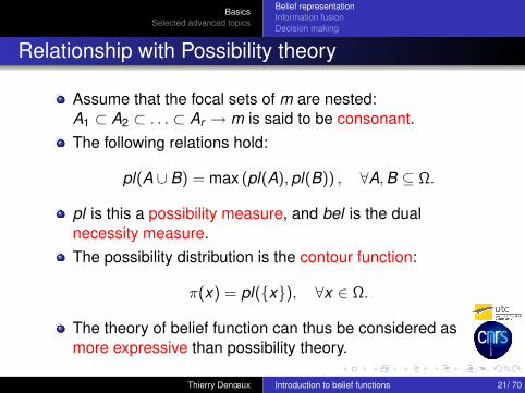
Relationship with Possibility theory

Assume that the focal sets of m are nested:A1 ⊂ A2 ⊂ . . . ⊂ Ar → m is said to be consonant.The following relations hold:

pl(A ∪ B) = max (pl(A),pl(B)) , ∀A,B ⊆ Ω.

pl is this a possibility measure, and bel is the dualnecessity measure.The possibility distribution is the contour function:

π(x) = pl(x), ∀x ∈ Ω.

The theory of belief function can thus be considered asmore expressive than possibility theory.




Outline






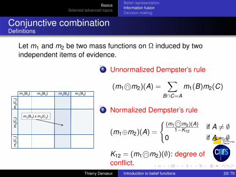
Conjunctive combinationDefinitions

Let m1 and m2 be two mass functions on Ω induced by twoindependent items of evidence.

m1(B1) m1(B2) m1(B3) m1(B4)

m2(

C 1)m

2(C 2)

m2(

C 3)

m1(B3) x m2(C2)

1 Unnormalized Dempster’s rule

(m1 ∩©m2)(A) =∑

B∩C=A

m1(B)m2(C)

2 Normalized Dempster’s rule

(m1⊕m2)(A) =

(m1 ∩©m2)(A)

1−K12if A 6= ∅

0 if A = ∅

K12 = (m1 ∩©m2)(∅): degree ofconflict.




Dempster’s ruleExample

We have m1(Peter , John) = 0.8, m1(Ω) = 0.2.New piece of evidence: a blond hair has been found.There is a probability 0.6 that the room has been cleanedbefore the crime→ m2(John,Mary) = 0.6, m2(Ω) = 0.4.

Peter , John Ω0.8 0.2

John,Mary John John,Mary0.6 0.48 0.12Ω Peter , John Ω

0.4 0.32 0.08




Dempster’s ruleJustification

(Θ1, P1)

ΩΓ1

drunk

not drunk Peter

John

Mary

(Θ2, P2)

Γ2

cleaned

not cleaned

Let (Θ1,P1, Γ1) and (Θ2,P2, Γ2) bethe multi-valued mappingsassociated to m1 and m2.If θ1 ∈ Θ1 and θ2 ∈ Θ2 both hold,then X ∈ Γ1(θ1) ∩ Γ2(θ2).If the two pieces of evidence areindependent, then this happens withprobability P1(θ1)P2(θ2).The normalized rule is obtainedafter conditioning on the event(θ1, θ2)|Γ1(θ1) ∩ Γ2(θ2) 6= ∅.




Dempster’s ruleProperties

Commutativity, associativity. Neutral element: mΩ.Generalization of intersection: if mA and mB arecategorical mass functions, then

mA ∩©mB = mA∩B

Generalization of probabilistic conditioning: if m is aBayesian mass function and mA is a categorical massfunction, then m ⊕mA is a Bayesian mass function thatcorresponding to the conditioning of m by A.Notations for conditioning (special case):

m ∩©mA = m(·|A), m ⊕mA = m∗(·|A).




Dempster’s ruleExpression using commonalities

Commonality function: let q : 2Ω → [0,1] be defined as

q(A) =∑B⊇A

m(B), ∀A ⊆ Ω.

Conversely,

m(A) =∑B⊇A

(−1)|B\A|q(B), ∀A ⊆ Ω.

Interpretation: q(A) = m(A|A), for any A ⊆ Ω.Expression of the unnormalized Dempster’s rule usingcommonalities:

(q1 ∩©q2)(A) = q1(A) · q2(A), ∀A ⊆ Ω.




TBM disjunctive ruleDefinition and justification

Let (Θ1,P1, Γ1) and (Θ2,P2, Γ2) be the multi-valuedmapping frameworks associated to two pieces of evidence.If interpretation θk ∈ Θk holds and piece of evidence k isreliable, then we can conclude that X ∈ Γk (θk ).If interpretation θ1 ∈ Θ1 and θ2 ∈ Θ2 both hold and weassume that at least one of the two pieces of evidence isreliable, then we can conclude that X ∈ Γ1(θ1) ∪ Γ2(θ2).This leads to the TBM disjunctive rule:

(m1 ∪©m2)(A) =∑

B∪C=A

m1(B)m2(C), ∀A ⊆ Ω




TBM disjunctive ruleProperties

Commutativity, associativity.Neutral element: m∅Let b = bel + m(∅) (implicability function). We have:

(b1 ∪©b2) = b1 · b2

De Morgan laws for ∩© and ∪©:

m1 ∪©m2 = m1 ∩©m2,

m1 ∩©m2 = m1 ∪©m2,

where m denotes the complement of m defined bym(A) = m(A) for all A ⊆ Ω.




Selecting a combination rule

All three rules ∩©, ⊕ and ∪© assume the pieces of evidenceto be independent.The conjunctive rules ∩© and ⊕ further assume that thepieces of evidence are both reliable;The TBM disjunctive rule ∪© only assumes that at least oneof the items of evidence combined is reliable (weakerassumption).∩© vs. ⊕:

∩© keeps track of the conflict between items of evidence:very useful in some applications.∩© also makes sense under the open-world assumption.The conflict increases with the number of combined massfunctions: normalization is often necessary at some point.

What to do with dependent items of evidence? → Cautiousrule




Outline






Decision makingProblem formulation

A decision problem can be formalized by defining:A set of acts A = a1, . . . ,as;A set of states of the world Ω;A loss function L : A× Ω→ R, such that L(a, ω) is the lossincurred if we select act a and the true state is ω.

Bayesian frameworkUncertainty on Ω is described by a probability measure P;Define the risk of each act a as the expected loss if a isselected:

R(a) = EP [L(a, ·)] =∑ω∈Ω

L(a, ω)P(ω).

Select an act with minimal risk.

Extension to the belief function framework?




Decision makingCompatible probabilities

Let m be a normalized mass function, and P(m) the set ofcompatible probability measures on Ω, i.e., the set of Pverifying

bel(A) ≤ P(A) ≤ pl(A), ∀A ⊆ Ω.

The lower and upper expected risk of each act a aredefined, respectively, as:

R(a) = Em[L(a, ·)] = infP∈P(m)

RP(a) =∑A⊆Ω

m(A) minω∈A

L(a, ω)

R(a) = Em[L(a, ·)] = supP∈P(m)

RP(a) =∑A⊆Ω

m(A) maxω∈A

L(a, ω)




Decision makingStrategies

For each act a we have a risk interval [R(a),R(a)]. How tocompare these intervals?Three strategies:

1 a is preferred to a′ iff R(a) ≤ R(a′);2 a is preferred to a′ iff R(a) ≤ R(a′) (optimistic strategy);3 a is preferred to a′ iff R(a) ≤ R(a′) (pessimistic strategy).

Strategy 1 yields only a partial preorder: a and a′ are notcomparable if R(a) > R(a′) and R(a′) > R(a).




Decision makingSpecial case

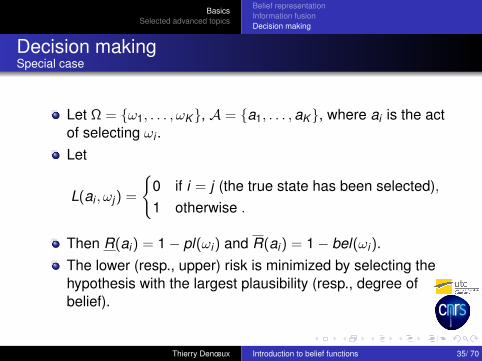
Let Ω = ω1, . . . , ωK, A = a1, . . . ,aK, where ai is the actof selecting ωi .Let

L(ai , ωj) =

0 if i = j (the true state has been selected),1 otherwise .

Then R(ai) = 1− pl(ωi) and R(ai) = 1− bel(ωi).The lower (resp., upper) risk is minimized by selecting thehypothesis with the largest plausibility (resp., degree ofbelief).




Decision makingComing back to Ellsberg’s paradox

We have m(r) = 1/3, m(b, y) = 2/3.

r b y R RA -100 0 0 -100/3 -100/3B 0 -100 0 -200/3 0C -100 0 -100 -100 -100/3D 0 -100 -100 -200/3 -200/3

The observed behavior (preferring A to B and D to C) isexplained by the pessimistic strategy.




Decision makingOther decision strategies

How to find a compromise between the pessimisticstrategy (minimizing the upper expected risk) and theoptimistic one (minimizing the lower expected risk)?Two approaches:

Hurwicz criterion: a is preferred to a′ iff Rρ(a) ≤ Rρ(a′) with

Rρ(a) = (1− ρ)R(a) + ρR(a).

and ρ ∈ [0,1] is a pessimism index describing the attitudeof the decision maker in the face of ambiguity.Pignistic transformation (Transferable Belief Model).




Decision makingTBM approach

The “Dutch book” argument: in order to avoid Dutch books(sequences of bets resulting in sure loss), we have to baseour decisions on a probability distribution on Ω.The TBM postulates that uncertain reasoning and decisionmaking are two fundamentally different operationsoccurring at two different levels:

Uncertain reasoning is performed at the credal level usingthe formalism of belief functions.Decision making is performed at the pignistic level, after them on Ω has been transformed into a probability measure.




Decision makingPignistic transformation

The pignistic transformation Bet transforms a normalizedmass function m into a probability measure Pm = Bet(m)as follows:

Pm(A) =∑∅6=B⊆Ω

m(B)|A ∩ B||B|

, ∀A ⊆ Ω.

It can be shown that bel(A) ≤ Pm(A) ≤ pl(A), hencePm ∈ P(m). Consequently,

R(a) ≤ RPm (a) ≤ R(a), ∀a ∈ A.




Decision makingExample

Let m(John) = 0.48, m(John,Mary) = 0.12,m(Peter , John) = 0.32, m(Ω) = 0.08.We have

Pm(John) = 0.48 +0.12

2+

0.322

+0.08

3≈ 0.73,

Pm(Peter) =0.32

2+

0.083≈ 0.19

Pm(Mary) =0.12

2+

0.083≈ 0.09



Informational orderingsCautious ruleMultidimensional belief functions

Outline






Informational comparison of belief functions

Let m1 et m2 be two mass functions on Ω.In what sense can we say that m1 is more informative(committed) than m2?Special case:

Let mA and mB be two categorical mass functions.mA is more committed than mB iff A ⊆ B.

Extension to arbitrary mass functions?




Plausibility and commonality orderings

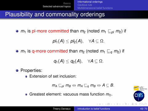
m1 is pl-more committed than m2 (noted m1 vpl m2) if

pl1(A) ≤ pl2(A), ∀A ⊆ Ω.

m1 is q-more committed than m2 (noted m1 vq m2) if

q1(A) ≤ q2(A), ∀A ⊆ Ω.

Properties:Extension of set inclusion:

mA vpl mB ⇔ mA vq mB ⇔ A ⊆ B.

Greatest element: vacuous mass function mΩ.




Strong (specialization) ordering

m1 is a specialization of m2 (noted m1 vs m2) if m1 can beobtained from m2 by distributing each mass m2(B) tosubsets of B:

m1(A) =∑B⊆Ω

S(A,B)m2(B), ∀A ⊆ Ω,

where S(A,B) = proportion of m2(B) transferred to A ⊆ B.S: specialization matrix.Properties:

Extension of set inclusion;Greatest element: mΩ;m1 vs m2 ⇒ m1 vpl m2 and m1 vq m2.




Least Commitment PrincipleDefinition

Definition (Least Commitment Principle)When several belief functions are compatible with a set ofconstraints, the least informative according to someinformational ordering (if it exists) should be selected.

A very powerful method for constructing belief functions!




Outline






Cautious ruleMotivations

The standard rules ∩©, ⊕ and ∪© assume the sources ofinformation to be independent, e.g.

experts with non overlapping experience/knowledge;non overlapping datasets.

What to do in case of non independent evidence?Describe the nature of the interaction between sources(difficult, requires a lot of information);Use a combination rule that tolerates redundancy in thecombined information.

Such rules can be derived from the LCP using suitableinformational orderings.




Cautious rulePrinciple

Two sources provide mass functions m1 and m2, and thesources are both considered to be reliable.After receiving these m1 and m2, the agent’s state of beliefshould be represented by a mass function m12 morecommitted than m1, and more committed than m2.Let Sx (m) be the set of mass functions m′ such thatm′ vx m, for some x ∈ pl ,q, s, · · · . We thus impose thatm12 ∈ Sx (m1) ∩ Sx (m2).According to the LCP, we should select the x-leastcommitted element in Sx (m1) ∩ Sx (m2), if it exists.




Cautious ruleProblem

The above approach works for special cases.Example (Dubois, Prade, Smets 2001): if m1 and m2 areconsonant, then the q-least committed element inSq(m1) ∩ Sq(m2) exists and it is unique: it is the consonantmass function with commonality function q12 = q1 ∧ q2.In general, neither existence nor uniqueness of a solutioncan be guaranteed with any of the x-orderings,x ∈ pl ,q, s.We need to define a new ordering relation.This ordering will be based on the (conjunctive) canonicaldecomposition of belief functions.




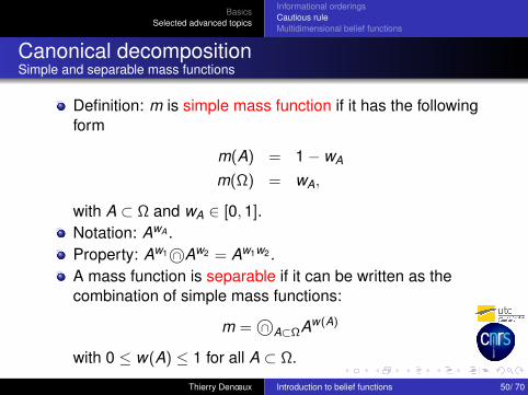
Canonical decompositionSimple and separable mass functions

Definition: m is simple mass function if it has the followingform

m(A) = 1− wA

m(Ω) = wA,

with A ⊂ Ω and wA ∈ [0,1].Notation: AwA .Property: Aw1 ∩©Aw2 = Aw1w2 .A mass function is separable if it can be written as thecombination of simple mass functions:

m = ∩©A⊂ΩAw(A)

with 0 ≤ w(A) ≤ 1 for all A ⊂ Ω.




Canonical decompositionSubtracting evidence

Let m12 = m1 ∩©m2. We have q12 = q1 · q2.Assume we no longer trust m2 and we wish to subtract itfrom m12.If m2 is non dogmatic (i.e. m2(Ω) > 0 or, equivalently,q2(A) > 0, ∀A), m1 can be retrieved as

q1 = q12/q2.

We note m1 = m12 6∩©m2.Remark: m1 6∩©m2 may not be a valid mass function!




Canonical decomposition

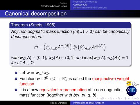
Theorem (Smets, 1995)

Any non dogmatic mass function (m(Ω) > 0) can be canonicallydecomposed as:

m =(∩©A⊂ΩAwC(A)

)6∩©(∩©A⊂ΩAwD(A)

)with wC(A) ∈ (0,1], wD(A) ∈ (0,1] and max(wC(A),wD(A)) = 1for all A ⊂ Ω.

Let w = wC/wD.Function w : 2Ω \Ω→ R∗+ is called the (conjunctive) weightfunction.It is a new equivalent representation of a non dogmaticmass function (together with bel , pl , q, b).




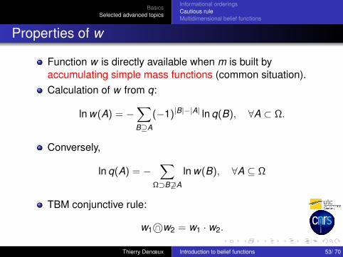
Properties of w

Function w is directly available when m is built byaccumulating simple mass functions (common situation).Calculation of w from q:

ln w(A) = −∑B⊇A

(−1)|B|−|A| ln q(B), ∀A ⊂ Ω.

Conversely,

ln q(A) = −∑

Ω⊃B 6⊇A

ln w(B), ∀A ⊆ Ω

TBM conjunctive rule:

w1 ∩©w2 = w1 · w2.




w-ordering

Let m1 and m2 be two non dogmatic mass functions. Wesay that m1 is w-more committed than m2 (denoted asm1 vw m2) if w1 ≤ w2.Interpretation: m1 = m2 ∩©m with m separable.Properties:

m1 vw m2 ⇒ m1 vs m2 ⇒

m1 vpl m2m1 vq m2,

mΩ is the only maximal element of vw :

mΩ vw m⇒ m = mΩ.




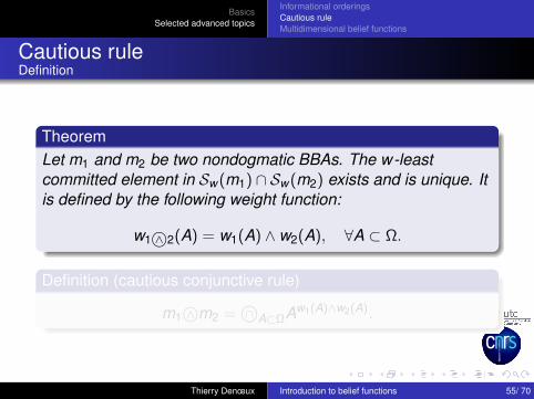
Cautious ruleDefinition

TheoremLet m1 and m2 be two nondogmatic BBAs. The w-leastcommitted element in Sw (m1) ∩ Sw (m2) exists and is unique. Itis defined by the following weight function:

w1 ∧©2(A) = w1(A) ∧ w2(A), ∀A ⊂ Ω.

Definition (cautious conjunctive rule)

m1 ∧©m2 = ∩©A⊂ΩAw1(A)∧w2(A).




Cautious ruleProperties

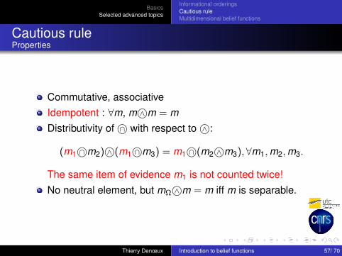
Commutative, associativeIdempotent : ∀m, m ∧©m = mDistributivity of ∩© with respect to ∧©:

(m1 ∩©m2) ∧©(m1 ∩©m3) = m1 ∩©(m2 ∧©m3),∀m1,m2,m3.

The same item of evidence m1 is not counted twice!No neutral element, but mΩ ∧©m = m iff m is separable.




Related rules

Normalized cautious rule:

(m1 ∧©∗m2)(A) =

(m1 ∧©m2)(A)

1−(m1 ∧©m2)(∅) if A 6= ∅0 if A = ∅.

Bold disjunctive rule:

m1 ∨©m2 = m1 ∧©m2.

Both ∧©∗ and ∨© are commutative, associative andidempotent.




Global picture

Six basic rules:

Sources independent dependent

All reliableopen world ∩© ∧©

closed world ⊕ ∧©∗At least one reliable ∪© ∨©




Outline






Multidimensional belief functionsMotivations

B

EEE

C

M

F G

E C

D X4 X5

X3 X2X1

A

X4

X3

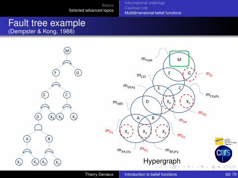
In many applications, we need toexpress uncertain information aboutseveral variables taking values indifferent domains.Example: fault tree (logical relationsbetween Boolean variables andprobabilistic or evidential informationabout elementary events).




Fault tree example(Dempster & Kong, 1988)

B

EEE

C

M

F G

E C

D X4 X5

X3 X2X1

A

X4

X3

M

F G

E C

D X4 X5

X3 X2X1

A B

mFGM

mGmCEF

mDEX4

mABD

mCX4X5

mAX1X3 mBX2X3

mX1

mX3

mX2

mX4

mX5

Hypergraph




Multidimensional belief functionsMarginalization, vacuous extension

Let X and Y be two variables defined on frames ΩX andΩY .Let ΩXY = ΩX × ΩY be the product frame.A mass function mΩXY on ΩXY can be seen as an uncertainrelation between variables X and Y .Two basic operations on product frames:

1 Express a joint mass function mΩXY in the coarser frame ΩXor ΩY (marginalization);

2 Express a marginal mass function mΩX on ΩX in the finerframe ΩXY (vacuous extension).




Marginalization

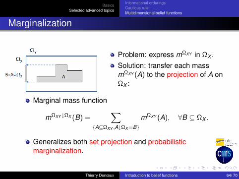
Problem: express mΩXY in ΩX .Solution: transfer each massmΩXY (A) to the projection of A onΩX :

Marginal mass function

mΩXY ↓ΩX (B) =∑

A⊆ΩXY ,A↓ΩX =B

mΩXY (A), ∀B ⊆ ΩX .

Generalizes both set projection and probabilisticmarginalization.




Vacuous extension

Problem: express mΩX in ΩXY .Solution: transfer each massmΩX (B) to the cylindrical extensionof B: B × ΩY .

Vacuous extension:

mΩX↑ΩXY (A) =

mΩX (B) if A = B × ΩY

0 otherwise.




Operations in product framesApplication to approximate reasoning

Assume that we have:Partial knowledge of X formalized as a mass function mΩX ;A joint mass function mΩXY representing an uncertainrelation between X and Y .

What can we say about Y?Solution:

mΩY =(

mΩX↑ΩXY ∩©mΩXY)↓ΩY

.

Infeasible with many variables and large frames ofdiscernment, but efficient algorithms exist to carry out theoperations in frames of minimal dimensions.




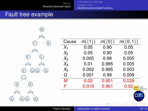
Fault tree example

B

EEE

C

M

F G

E C

D X4 X5

X3 X2X1

A

X4

X3

Cause m(1) m(0) m(0,1)X1 0.05 0.90 0.05X2 0.05 0.90 0.05X3 0.005 0.99 0.005X4 0.01 0.985 0.005X5 0.002 0.995 0.003G 0.001 0.99 0.009M 0.02 0.951 0.029F 0.019 0.961 0.02




Summary

The theory of belief function: a very general formalism forrepresenting imprecision and uncertainty that extends bothprobabilistic and set-theoretic frameworks:

Belief functions can be seen both as generalized sets andas generalized probability measures;Reasoning mechanisms extend both set-theoretic notions(intersection, union, cylindrical extension, inclusionrelations, etc.) and probabilistic notions (conditioning,marginalization, Bayes theorem, stochastic ordering, etc.).

The theory of belief function can also be seen as moregeneral than Possibility theory (possibility measures areparticular plausibility functions).


References

References Icf. http://www.hds.utc.fr/˜tdenoeux

G. Shafer.A mathematical theory of evidence. Princeton University Press,Princeton, N.J., 1976.

Ph. Smets and R. Kennes.The Transferable Belief Model.Artificial Intelligence, 66:191-243, 1994.

D. Dubois and H. Prade.A set-theoretic view of belief functions: logical operations andapproximations by fuzzy sets.International Journal of General Systems, 12(3):193-226, 1986.


References

References IIcf. http://www.hds.utc.fr/˜tdenoeux

T. Denœux.

Analysis of evidence-theoretic decision rules for patternclassification.

Pattern Recognition, 30(7):1095-1107, 1997.

T. Denœux.

Conjunctive and Disjunctive Combination of Belief FunctionsInduced by Non Distinct Bodies of Evidence.

Artificial Intelligence, Vol. 172, pages 234-264, 2008.


Introduction to belief functions - Gipsa-lab · A belief function may be viewed both as...

Documents

Transcript of Introduction to belief functions - Gipsa-lab · A belief function may be viewed both as...