Introduction to Asymptotic Approximation by Holmes

8/14/2019 Introduction to Asymptotic Approximation by Holmes

http://slidepdf.com/reader/full/introduction-to-asymptotic-approximation-by-holmes 1/57



2 1 Introduction to Asymptotic Approximations

___

Figure 1.1 Schematic of solution x0 (t ) given in ( 1.2). This solution comes from thelinearization of ( 1.1) and corresponds to the motion in a uniform gravitational eld

this reduction is that it is unclear how to determine a correction to theapproximate solution in ( 1.2). This is worth knowing since we would then be

able to get a measure of the error made in using ( 1.2) as an approximationand it would also be possible to see just how the nonlinear nature of theoriginal problem affects the motion of the object.

To make the reduction process more systematic, it is rst necessary toscale the variables. To do this, let τ = t/t c and y(τ ) = x(t)/x c , where tcis a characteristic time for the problem and xc is a characteristic value forthe solution. We have a lot of freedom in picking these constants, but theyshould be representative of the situation under consideration. Based on whatis shown in Fig. 1.1, we take tc = v0 /g and xc = v2

0 /g . Doing this the problemtransforms into the following:

d2 ydτ 2

= − 1

(1 + εy)2 , for 0 < τ, (1.3)

wherey(0) = 0 and y (0) = 1 . (1.4)

In (1.3), the parameter ε = v20 /Rg is dimensionless and its value is important

because it gives us a measure of how high the projectile gets in comparisonto the radius of the Earth. In terms of the function x0(t) it can be seen fromFig. 1.1 that ε/ 2 is the ratio of the maximum height of the projectile to theradius of the Earth. Assuming R = 4 ,000 mi, then ε ≈1.5 ×10− 9v2

0 s2 / ft2 . Itwould therefore appear that if v0 is much less than 10 3 ft/s, then ( 1.2) is areasonably good approximation to the solution. We can verify this assertionby reconstructing the rst-order approximation in ( 1.2). This can be done byassuming that the dependence of the solution on ε can be determined using aTaylor series expansion about ε = 0. In other words, for small ε it is assumedthat

y

∼

y0(τ ) + εy1(τ ) +

· · · .

The rst term in this expansion is the scaled version of x0 , and this will beshown later (Sect. 1.6). What is important is that with this approach it ispossible to estimate how well y0 approximates the solution of ( 1.3), (1.4) by

http://-/?-

http://-/?-

http://-/?-

http://-/?-

http://-/?-

http://-/?-

http://-/?-

http://-/?-

http://-/?-

http://-/?-

http://-/?-

http://-/?-

http://-/?-

http://-/?-

http://-/?-

http://-/?-

http://-/?-

http://-/?-

http://-/?-

http://-/?-

http://-/?-

http://-/?-

http://-/?-

http://-/?-



1.2 Taylor’s Theorem and l’Hospital’s Rule 3

nding y1 . The method of deriving the rst-order approximation ( y0) andits correction ( y1) is not difficult, but we rst need to put the denitionof an asymptotic approximation on a rm foundation. Readers interestedin investigating the ideas underlying the nondimensionalization of a physical

problem and some of the theory underlying dimensional analysis may consultHolmes (2009).

1.2 Taylor’s Theorem and l’Hospital’s Rule

As in the preceding example, we will typically end up expanding functions inpowers of ε. Given a function f (ε), one of the most important tools for doing

this is Taylor’s theorem. This is a well-known result, but for completeness itis stated below.

Theorem 1.1. Given a function f (ε), suppose its (n + 1) st derivative f (n +1)

is continuous for εa < ε < ε b. In this case, if ε0 and ε are points in the interval (εa , εb), then

f (ε) = f (ε0) + ( ε −ε0)f (ε0) + · · ·+ 1n!

(ε −ε0)n f (n ) (ε0) + Rn +1 , (1.5)

where Rn +1 =

1(n + 1)!

(ε −ε0)n +1 f (n +1) (ξ ) (1.6)

and ξ is a point between ε0 and ε.

This result is useful because if the rst n + 1 terms from the Taylor seriesare used as an approximation of f (ε), then it is possible to estimate the errorusing (1.6).

A short list of Taylor series expansions that will prove useful in this book

is given in Appendix A. Examples using this list are given below.

Examples

1. Find the rst three terms in the expansion of f (ε) = sin(e ε ) for ε0 = 0.

Given that f = e ε cos(eε ) and f = e ε (cos(e ε ) −sin(e ε )), it follows that

f (ε) = sin(1) + ε cos(1) + 1

2ε2(cos(1)

−sin(1)) +

· · · .

2. Find the rst three terms in the Taylor expansion of f (ε) = e ε / (1 −ε) forε0 = 0.

http://-/?-

http://-/?-




There are a couple of ways this can be done. One is the direct methodusing (1.5), the other is to multiply the series for e ε with the series for1/ (1 −ε). To use the direct method, note that

f (ε) = eε

1 −ε + eε

(1 −ε)2

andf (ε) =

eε

1 −ε +

2eε

(1 −ε)2 + 2eε

(1 −ε)3 .

Evaluating these at ε = 0 it follows from (1.5) that a three-term Taylorexpansion is

f (ε) = 1 + 2 ε + 5 ε2 + · · · .

Another useful result is l’Hospital’s rule, which concerns the value of thelimit of the ratio of two functions.

Theorem 1.2. Suppose f (ε) and φ(ε) are differentiable on the interval (ε0 , εb) and φ (ε) = 0 in this interval. Also suppose

limε↓ ε 0

f (ε)φ (ε)

= A,

where −∞ ≤A ≤ ∞. In this case,

limε↓ ε 0

f (ε)φ(ε)

= A

if either one of the following conditions holds:

1. f →0 and φ →0 as ε ↓ε0 , or

2. φ

→ ∞ as ε

↓ε0 .

The proofs of these two theorems and some of their consequences can befound in Rudin (1964).

1.3 Order Symbols

To dene an asymptotic approximation, we rst need to introduce order, orLandau, symbols .1 The reason for this is that we will be interested in howfunctions behave as a parameter, typically ε, becomes small. For example,1 These symbols were rst introduced by Bachmann (1894), and then Landau (1909)popularized their use. For this reason they are sometimes called Bachmann–Landausymbols.

http://-/?-

http://-/?-

http://-/?-

http://-/?-

http://-/?-

http://-/?-

http://-/?-



1.3 Order Symbols 5

the function φ(ε) = ε does not converge to zero as fast as f (ε) = ε2 whenε →0, and we need a notation to denote this fact.

Denition 1.1.

1. f = O(φ) as ε ↓ε0 means that there are constants k0 and ε1 (independentof ε) so that

|f (ε)| ≤k0|φ(ε)| for ε0 < ε < ε 1 .

We say that “ f is big Oh of φ” as ε ↓ε0 .

2. f = o(φ) as ε ↓ε0 means that for every positive δ there is an ε2 (indepen-dent of ε) so that

|f (ε)| ≤δ |φ(ε)| for ε0 < ε < ε 2 .We say that “ f is little oh of φ” as ε ↓ε0 .

These denitions may seem cumbersome, but they usually are not hardto apply. However, there are other ways to determine the correct order. Of particular interest is the case where φ is not zero near ε0 (i.e., φ = 0 if ε0 < ε < ε β for some εβ > ε 0). In this case we have that f = O(φ) if theratio |f /φ | is bounded for ε near ε0 . Other, perhaps more useful, tests areidentied in the next result.

Theorem 1.3.

1. If

limε↓ ε 0

f (ε)φ(ε)

= L, (1.7)

where −∞< L < ∞, then f = O(φ) as ε ↓ε0 .

2. If

limε↓ ε 0

f (ε)φ(ε)

= 0 , (1.8)

then f = o(φ) as ε ↓ε0 .

The proofs of these statements follow directly from the denition of a limitand are left to the reader.

Examples (for ε ↓ 0)

1. Suppose f = ε2 . Also, let φ1 = ε and φ2 = −3ε2 + 5 ε6 . In this case,

limε↓ 0

f φ1

= 0 ⇒ f = o(φ1 )




andlimε↓ 0

f φ2

= −13 ⇒ f = O(φ2 ).

2. If f = ε sin(1 + 1 /ε ) and φ = ε, then the limit in the preceding theoremdoes not exist. However, |f /φ | ≤1 for 0 < ε , and so from the denition itfollows that f = O(φ).

3. If f (ε) = sin( ε) then, using Taylor’s theorem, f = ε − 12 ε2 sin(ξ ). Thus,

limε ↓0(f /ε ) = 1, and from this it follows that f = O(ε).

4. If f = e − 1/ε then, using l’Hospital’s rule, f = o(εα ) for all values of α . Wesay in this case that f is transcendentally small with respect to the powerfunctions εα .

Some properties of order symbols are examined in the exercises. Threethat are worth mentioning are the following (the symbol ⇔ stands for thestatement “if and only if”):

(a) f = O(1) as ε ↓ε0 ⇔f is bounded as ε ↓ε0 .

(b) f = o(1) as ε ↓ε0 ⇔f →0 as ε ↓ε0 .

(c) f = o(φ) as ε ↓ε0 ⇒f = O(φ) as ε ↓ε0 (but not vice versa).

The proofs of these statements are straightforward and are left to the reader.Some of the other basic properties of these symbols are given in Exercises 1.2and 1.3.

Two symbols we will use occasionally are and ≈. When we say thatf (ε) φ(ε), we mean that f = o(φ), and the statement that ε 1, or thatε is small, means ε ↓0. The symbol ≈ does not have a precise denition andit is used simply to designate an approximate numerical value. An exampleof this is the statement that π ≈3.14.

Exercises

1.1. (a) What values of α, if any, yield f = O(εα ) as ε ↓0: (i) f = √ 1 + ε2 ,(ii) f = ε sin(ε), (iii) f = (1 −eε )− 1 , (iv) f = ln(1 + ε), (v) f = ε ln(ε),(vi) f = sin(1 /ε ), (vii) f = √ x + ε, where 0 ≤x ≤1?

(b) For the functions listed in (a) what values of α, if any, yield f = o(εα )as ε ↓0?

1.2. In this problem it is assumed that ε ↓0.(a) Show f = O(εα ) ⇒f = o(εβ ) for any β < α .(b) Show that if f = O(g), then f α = O(gα ) for any positive α. Give an

example to show that this result is not necessarily true if α is negative.

http://-/?-

http://-/?-

http://-/?-

http://-/?-

http://-/?-



1.4 Asymptotic Approximations 7

(c) Give an example to show that f = O(g) does not necessarily mean thatef = O(eg ).

1.3. This problem establishes some of the basic properties of the order sym-bols, some of which are used extensively in this book. The limit assumed hereis ε ↓0.(a) If f = o(g) and g = O(h), or if f = O(g) and g = o(h), then show that

f = o(h). Note that this result can be written as o(O(h)) = O(o(h)) =o(h).

(b) Assuming f = O(φ1 ) and g = O(φ2 ), show that f + g = O(|φ1 | + |φ2 |).Also, explain why the absolute signs are necessary. Note that this resultcan be written as O(f ) + O(g) = O(|f |+ |g|).(c) Assuming f = O(φ1 ) and g = O(φ2 ), show that fg = O(φ1 φ2 ). Thisresult can be written as O(f )O(g) = O(fg ).

(d) Show that O(O(f )) = O(f ).(e) Show that O(f )o(g) = o(f )o(g) = o(fg ).

1.4. Occasionally it is useful to state the order of a function more precisely.One way to do this is to say f = Os(φ) as ε ↓ε0 ⇔ f = O(φ) but f = o(φ)as ε ↓ε0 .(a) What values of α, if any, yield f = Os(εα ) as ε ↓ 0? (i) f = ε sin(ε), (ii)

f = (1 −eε )− 1 , (iii) f = ln(1 + ε), (iv) f = ε ln(ε), (v) f = sin(1 /ε ).(b) Suppose the limit in ( 1.7) exists. In this case, show that f = Os (φ) as

ε ↓ε0 ⇔0 < limε↓ ε 0

|f /φ | < ∞.1.5. Suppose f = o(φ) for small ε, where f and φ are continuous.(a) Give an example to show that it is not necessarily true that

ε

0f dε = o

ε

0φdε .

(b) Show that

ε

0

f dε = o

ε

0 |φ

|dε .

1.4 Asymptotic Approximations

Our objective is to construct approximations to the solutions of differentialequations. It is therefore important that we state exactly what we meanby an approximation. To introduce this idea, suppose we are interested innding an approximation of f (ε) = ε2 + ε5 for ε close to zero. Becauseε5 ε2 , a reasonable approximation is f (ε) ≈ε2 . On the other hand, a lousyapproximation is f (ε) ≈ 2

3 ε2 . This is lousy even though the error f (ε) − 23 ε2

goes to zero as ε ↓ 0. The problem with this “lousy approximation” is thatthe error is of the same order as the function we are using to approximatef (ε). This observation gives rise to the following denition.

http://-/?-

http://-/?-




x-axis

F u n c t i o n

0 0.2 0.4 0.6 0.8 10

0.5

1

FunctionAsymptotic Approximation

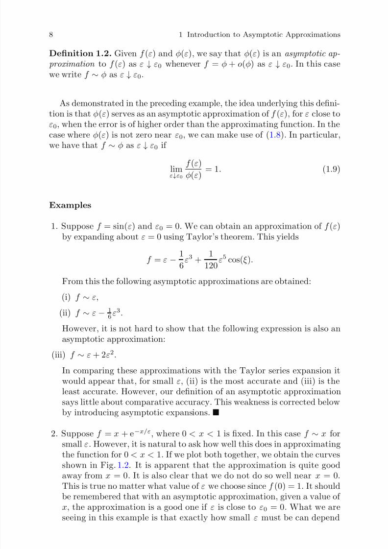
Figure 1.2 Comparison between the function f = x + e − x/ε and its asymptoticapproximation f ∼ x. Note that the two functions are essentially indistinguishableeverywhere except near x = 0. In this plot, ε = 10 − 2

on x (the closer we are to x = 0, the smaller ε must be). In later sectionswe will refer to this situation as a case where the approximation is notuniformly valid on the interval 0 < x < 1.

3. Consider the function f = sin( πx )+ ε3 for 0 ≤x ≤ 12 . For small ε it might

seem reasonable to expect that f ∼sin(πx ). For this to hold it is requiredthat f −sin(πx ) = o(sin( πx )) as ε ↓ 0. If x = 0, then this is true sincelimε↓ 0(ε3 / sin(πx )) = 0. However, at x = 0 this requirement does not holdsince sin(0) = 0. Therefore, sin( πx ) is not an asymptotic approximationof f over the entire interval 0 ≤ x ≤ 1

2 . This problem of using an ap-proximating function whose zeros do not agree with the original functionis one that we will come across on numerous occasions. Usually it is acomplication we will not worry a great deal about because the correctionis relatively small. For instance, in this example the correction is O(ε3 )while everywhere else the function is O(1). This is not true for the cor-rection that is needed to x the approximation in the previous example.There the correction at, or very near, x = 0 is O(1), and this is the same

order as the value of the function through the rest of the interval. We aretherefore not able to ignore the problem at x = 0; how to deal with thisis the subject of Chap.2.

1.4.1 Asymptotic Expansions

Two observations that come from the preceding examples are that an asymp-totic approximation is not unique, and it also does not say much about theaccuracy of the approximation. To address these shortcomings, we need tointroduce more structure into the formulation. In the preceding examples,the sequence 1, ε, ε2 , ε3 , . . . was used in the expansion of the function, but




other, usually more interesting, sequences also arise. In preparation for this,we have the following denitions, which are due to Poincare (1886).

Denition 1.3.

1. The functions φ1 (ε), φ2(ε), . . . form an asymptotic sequence , or are well ordered , as ε ↓ε0 if and only if φm +1 = o(φm ) as ε ↓ε0 for all m.

2. If φ1 (ε), φ2(ε), . . . is an asymptotic sequence, then f (ε) has an asymptotic expansion to n terms, with respect to this sequence, if and only if

f =m

k=1

ak φk + o(φm ) for m = 1 , 2, . . . , n as ε ↓ε0 , (1.10)

where the ak are independent of ε. In this case we write

f ∼a1φ1 (ε) + a2φ2 (ε) + · · ·+ an φn (ε) as ε ↓ε0 . (1.11)

The φk are called the scale or gauge or basis functions.

To make use of this denition, we need to have some idea of what scalefunctions are available. We will run across a wide variety in this book, but acouple of our favorites will turn out to be the following ones:

1. φ1 = ( ε −ε0)α , φ2 = ( ε −ε0)β , φ3 = ( ε −ε0)γ , . . ., where α < β < γ < · · ·.2. φ1 = 1, φ2 = e − 1/ε , φ3 = e − 2/ε , . . . .

The rst of these is simply a generalization of the power series functions, andthe second sequence is useful when we have to describe exponentially smallfunctions. The verication that these do indeed form asymptotic sequencesis left to the reader.

Now comes the harder question. Given a function f (ε), how do we nd anasymptotic expansion of it? The most commonly used methods include em-ploying one of the following: (1) Taylor’s theorem, (2) l’Hospital’s rule, or (3)an educated guess. The last one usually relies on an intuitive understandingof the problem and, many times, on luck. The other two methods are moreroutine and are illustrated in the examples below.

Taylor’s theorem is a particularly useful tool because if the function issmooth enough to let us expand about the point ε = ε0 , then any one of the resulting Taylor polynomials can be used as an asymptotic expansion(for ε ↓ε0). Moreover, Taylor’s theorem enables us to analyze the error very

easily.




Examples (for ε 1)

1. To nd a three-term expansion of e ε , we use Taylor’s theorem to obtain

eε = 1 + ε + 12ε2 + 13 ε3 + · · ·∼1 + ε +

12

ε2 .

2. Finding the rst two terms in the expansion of f (ε) = cos( ε)/ε requiresan extension of Taylor’s theorem because the function is not dened atε = 0. One way this can be done is to factor out the singular part of f (ε)and apply Taylor’s theorem to the remaining regular portion. The singularpart here is 1 /ε , and the regular part is cos( ε). Using the expansion forcos(ε) in Appendix A we obtain

f (ε)∼ 1ε

1 − 12

ε2 + · · ·∼

1ε −

12

ε.

As expected, the expansion, like the function, is not dened at ε = 0.

3. To nd a two-term expansion of

f (ε) = √ 1 + εsin(√ ε)

,

note that√ 1 + ε = 1 +

12

ε + · · ·and

sin(√ ε) = ε1/ 2 − 16

ε3/ 2 + · · · .Consequently,

f (ε)∼ 1 + 1

2 ε + · · ·ε1/ 2 − 1

6 ε3/ 2 + · · · =

1ε1/ 2

1 + 12 ε + · · ·

1 − 16 ε + · · ·

∼ 1ε1/ 2 1 +

12

ε + · · · 1 + 16

ε + · · ·

∼ 1ε1/ 2 1 +

13

ε .

A nice aspect about using Taylor’s theorem is that the scale functions donot have to be specied ahead of time. This differs from the next procedure,




which requires the specication of the scale functions before constructing theexpansion.

To describe the second procedure for constructing an asymptotic expan-sion, suppose the scale functions φ1 , φ2 , . . . are given, and the expansion of

the function has the form f ∼ a1φ1 (ε) + a2φ2 (ε) + · · ·. From the precedingdenition, this means that f = a1φ1 + o(φ1 ). Assuming we can divide byφ1 , we get limε↓ ε 0 (f /φ 1) = a1 . This gives us the value of a1 , and with thisinformation we can determine a2 by noting f = a1φ1 + a2φ2 + o(φ2 ). Thus,limε↓ ε 0 [(f −a1φ1 )/φ 2] = a2 . This idea can be used to calculate the othercoefficients of the expansion, and one obtains the following formulas:

a1 = limε↓ ε 0

f φ1

, (1.12)

a2 = limε↓ ε 0f −a1φ1

φ2, (1.13)

a3 = limε↓ ε 0

f −a1φ1 −a2φ2

φ3. (1.14)

This assumes that the scale functions are nonzero for ε near ε0 and that eachof the limits exists. If this is the case, then the preceding formulas for the akshow that the asymptotic expansion is unique.

Example

Suppose φ1 = 1, φ2 = ε, φ3 = ε2 , . . ., and

f (ε) = 11 + ε

+ e − 1/ε .

From the preceding limit formulas we have that

a1 = limε ↓0

f 1 = 1 ,

a2 = limε ↓0

f −1ε

= limε ↓0

−11 + ε

+ 1ε

e− 1/ε = −1,

a3 = limε ↓0

f −1 + εε2 = lim

ε↓ 0

11 + ε

+ 1ε2 e− 1/ε = 1 .

Thus, f ∼1 −ε + ε2 + · · ·. What is interesting here is that the exponentialmakes absolutely no contribution to this expansion. This is because e − 1/ε =

o(εα

) for all values of α; in other words, the exponential decays so quicklyto zero that any power function considers it to be zero. In this case, we saythat this exponential function is transcendentally small with respect to thesescale functions.




As seen in the previous example, two functions can have the sameasymptotic expansion. In particular, using the power series functions φ0 = 1,φ1 = ε, φ2 = ε2 , . . . one obtains the same expansion as in the previousexample for any of the following functions:

(i) f 1 = tanh(1 /ε )

1 + ε ,

(ii) f 2 = 1 + e− 1/ε

1 + ε ,

(iii) f 3 = 11 + ε

+ ε100 sech(−1/ε ).

This observation brings up the idea of asymptotic equality, or asymptoticequivalence, with respect to a given sequence φ1 , φ2 , φ3 , . . .. We say that twofunctions f and g are asymptotically equal to n terms if f −g = o(φn ) asε ↓ε0 .

1.4.2 Accuracy Versus Convergenceof an Asymptotic Series

It is not unusual to expect that to improve the accuracy of an asymptoticexpansion, it is simply necessary to include more terms. This is what happenswith Taylor series expansions, where in theory one should be able to obtainas accurate a result as desired by simply adding together enough terms. How-ever, with an asymptotic expansion this is not necessarily true. The reasonis that an asymptotic expansion only makes a statement about the series inthe limit of ε ↓ ε0 , whereas increasing the number of terms is saying some-thing about the series as n → ∞. In fact, an asymptotic expansion neednot converge! Moreover, even if it converges, it does not have to convergeto the function that was expanded! These two observations may seem to bemajor aws in our denition of an asymptotic expansion, but they are, infact, attributes that we will take great advantage of throughout this book.

A demonstration that a convergent asymptotic expansion need not con-verge to the function that was expanded can be found in the last example.It is not hard to show that the asymptotic series converges to the function(1 + ε)− 1 . This is clearly not equal to the original function since it is missingthe exponential term.

A well-known example of a divergent asymptotic expansion arises with theBessel function J 0(z), which is dened as

J 0(z) =∞

k=0

(−1)k z2k

22k (k!)2 . (1.15)




0 20 40 60 80 100Number of Terms

10 8

10 0

10 −8

10 −16

E

r r o r

SeriesAsymptotic Approximation

'

Figure 1.3 The error when using the convergent series (1.15 ) or the asymptoticseries (1.16 ) to determine the value of the function f (ε) = J 0 (ε− 1 ) for ε = 1

15 . Thevalues are given as a function of the number of terms used

If we let f (ε) = J 0( 1ε ), then it can be shown that an asymptotic expansion

of f (ε) for small ε is (Abramowitz and Stegun, 1972)

f ∼ 2επ

α cos1ε −

π4

+ β sin1ε −

π4

, (1.16)

whereα∼1 −

1 ·32ε2

2! 82 + 1 ·32 ·52 ·72ε4

4! 84 + · · · (1.17)

andβ ∼

ε8 −

1 ·32 ·52ε3

3! 83 + · · · . (1.18)

It is not hard to show that the series expansions in ( 1.17) and (1.18) aredivergent for all nonzero values of ε (Exercise 1.14). To see just how well adivergent series like ( 1.16) can approximate the function f (ε), the errors inusing (1.15) and (1.16)–(1.18) are shown in Fig. 1.3 for ε = 1 / 15. What isimmediately apparent is that the asymptotic approximation does very wellusing only 1 or 2 terms, while the convergent series needs to include morethan 20 terms to achieve the same error. If a smaller value of ε is used, thenthe situation is even more pronounced, eventually getting to the point thatit is essentially impossible to calculate the value of the Bessel function usingthe series representation since so many terms are needed.

The preceding observations concerning convergence should always be keptin mind when using asymptotic expansions. Also, it should be pointed outthat asymptotic approximations are most valuable when they can give in-sights into the structure of a solution or the physics of the problem understudy. If decimal place accuracy is desired, then numerical methods, or per-

haps numerical methods combined with an asymptotic solution, are probablyworth considering.

The ideas underlying an asymptotic approximation are so natural thatthey are found in some of the earliest work in mathematics. The basis of the denitions given here can be traced back to at least Legendre (1825).

http://-/?-

http://-/?-

http://-/?-

http://-/?-

http://-/?-

http://-/?-

http://-/?-

http://-/?-

http://-/?-

http://-/?-

http://-/?-

http://-/?-

http://-/?-

http://-/?-

http://-/?-

http://-/?-

http://-/?-

http://-/?-

http://-/?-

http://-/?-

http://-/?-

http://-/?-

http://-/?-

http://-/?-




In his Traite des Fonctions Elliptiques he considered approximating a functionwith a series where the error committed using the rst n terms is of the sameorder as the ( n + 1)st term. He referred to this as a semiconvergent series.This is a poor choice of words since an asymptotic series need not converge.

Somewhat earlier than this, Laplace (1812) had found use for asymptoticseries to be able to evaluate certain special functions because the standardseries expansions converged so slowly. He considered the fact that they did notconverge to be “inconvenient,” an interesting attitude that generally leads todisastrous results. The most signicant contribution to the subject was madeby Poincare (1886). He was able to make sense of the numerous divergentseries solutions of differential equations that had been found up to that timeby introducing the concept of an asymptotic expansion. His ideas form thebasis of our development. It is interesting that his paper actually marked the

modern beginnings of two areas in mathematics: the asymptotic solution of adifferential equation and the study of divergent series. The latter can also becalled the theory of summability of a divergent series, and the books by Ford(1916) and Hardy (1954) are good references in this area. However, if thereader has not heard of this particular subject, it is not surprising becauseit has since died of natural causes. Readers interested in the early history of the development of asymptotic approximations may consult the reviews byMcHugh (1971) and Schlissel (1977a).

1.4.3 Manipulating Asymptotic Expansions

It is not hard to show that two asymptotic expansions can be added togetherterm by term, assuming that the same basis functions are used for bothexpansions. Multiplication is also relatively straightforward, albeit more te-dious and limited to asymptotic sequences that can be ordered in particularways (e.g., Exercise 1.12). What is not completely clear is whether or notan asymptotic approximation can be differentiated (assuming the functionsinvolved are smooth). To be more specic, suppose we know that

f (x, ε )∼φ1 (x, ε ) + φ2 (x, ε ) as ε ↓ε0 . (1.19)

What is of interest is whether or not it is true that

ddx

f (x, ε )∼ ddx

φ1 (x, ε ) + ddx

φ2 (x, ε ) as ε ↓ε0 . (1.20)

Based on the conjecture that things will go wrong if at all possible, the only

possible answer to the preceding question is that, no, it is not always true.To give an example, let f (x, ε ) = e − x/ε sin(ex/ε ). For small ε one nds that,for 0 < x < 1,

f ∼0 + 0 ·ε + 0 ·ε2 + · · · . (1.21)

http://-/?-

http://-/?-




However, the function

ddx

f (x, ε ) = −1ε

e− x/ε sin(ex/ε ) + 1ε

cos(ex/ε )

does not even have an expansion in terms of the scale functions used in ( 1.21).Another problem is that even if φ1 and φ2 are well ordered, their derivatives

may not be. For example, letting φ1 = 1 + x and φ2 = ε sin(x/ε ), for 0 ≤x ≤1, then φ2 = o(φ1 ) for ε small, but dd x φ1 and d

dx φ2 are not well ordered.Thus, the question that we need to address is when can we differentiate anexpansion? Well, the answer to this is that if

f (x, ε )∼a1 (x)φ1 (ε) + a2(x)φ2 (ε) as ε ↓ε0 , (1.22)

and if ddx

f (x, ε )∼b1(x)φ1 (ε) + b2(x)φ2 (ε) as ε ↓ε0 , (1.23)

then bk = ddx ak [i.e., the expansion for d

dx f can be obtained by differentiatingthe expansion of f (x, ε ) term by term]. Throughout this book, given ( 1.22),we will automatically assume that ( 1.23) also holds.

The other operation we will have use for is integration, and in this casethe situation is better. If the expansion of a function is as given in (1.22) andall the functions involved are integrable, then

b

af (x, ε )dx∼ b

aa1(x)dx φ1 (ε) + b

aa2(x)dx φ2 (ε) as ε ↓ε0 .

(1.24)It goes without saying here that the interval a ≤ x ≤ b must be within theset of x where (1.22) holds.

Examples

1. Find the rst two terms in the expansion of f (ε) = 1

0 eεx 2

dx.

Given that e εx 2

∼1 + εx 2 + · · ·, and this holds for 0 ≤x ≤1, then

f (ε)∼ 1

0(1 + εx 2 + · · ·)dx

= 1 + 13

ε + · · · .

2. Find the rst two terms in the expansion of

f (ε) = 1

0

dxε2 + x2 .

http://-/?-

http://-/?-

http://-/?-

http://-/?-

http://-/?-

http://-/?-

http://-/?-

http://-/?-

http://-/?-

http://-/?-

http://-/?-




For 0 < x ≤1 the integrand has the expansion

1ε2 + x2 ∼

1x2 −

ε2

x4 + · · · . (1.25)

Unfortunately, the terms in this expansion are not integrable over theinterval 0 ≤ x ≤ 1. This can be avoided by taking the easy way outand simply calculating the integral and then expanding the result. Thisproduces the following:

f (ε) = 1ε

arctan1ε

= 1ε

π2 −arctan( ε)

∼ π2ε −1 + 1

3ε2 + · · · . (1.26)

For more complicated integrals it is not possible to carry out the inte-gration, and this brings up the question of whether we can obtain ( 1.26)some other way. To answer this, note that for ( 1.25) to be well ordered werequire ε2 /x 4 1/x 2 , that is, ε x. Therefore, to use ( 1.25), we write

f (ε) =

δ

0

dx

ε2

+ x2 +

1

δ

dx

ε2

+ x2 ,

where ε δ 1. The idea here is that the rst integral is over a smallinterval containing the singularity, and the second integral is over the re-mainder of the interval where we can use ( 1.25). With this

1

δ

dxε2 + x2 ∼

1

δ

1x2 −

ε2

x4 + · · · dx

=

−1 +

13

ε2 + 1δ

−

ε3

3δ 3 +

· · ·and

δ

0

dxε2 + x2 =

1ε

arctanδ ε

= π2ε −

1δ

+ · · · .Adding these together we obtain ( 1.26).

3. Find the rst two terms in the expansion of

f (ε) = π/ 3

0

dxε2 + sin x

.

http://-/?-

http://-/?-

http://-/?-

http://-/?-

http://-/?-

http://-/?-

http://-/?-

http://-/?-

http://-/?-

http://-/?-




Like the last example, this has a nonintegrable singularity at x = 0 whenε = 0. This is because for x near zero, sin x = x + O(x3 ), and 1 /x is notintegrable when one of the endpoints is x = 0. Consequently, as before, wewill split the interval. First, note that

1ε2 + sin x ∼

1sin x

1 − ε2

sin x + · · · .

For this to be well ordered near x = 0 we require that ε2/ sin x 1, thatis, ε2 x. So, we write

f (ε) = δ

0

dxε2 + sin x

+ π/ 3

δ

dxε2 + sin x

,

where ε2 δ 1. With this

π/ 3

δ

dxε2 + sin x ∼

π/ 3

δ

1sin x

1 − ε2

sin x + · · · dx

= ln13√ 3 −ln tan

δ 2

+ ε2 13√ 3 −cot( δ ) + · · ·

∼ln23√ 3 +

13√ 3 ε2 − ln(δ ) +

ε2

δ +

112

δ 2 + · · ·and, setting η = δ/ε 2 ,

δ

0

dx

ε2 + sin x

= ε2

η

0

d r

ε2 + sin( ε

2r )

∼ ε2

η

0

d r

ε2 + ε

2r −

16 ε

6r

3 + · · ·

∼ η

0

11 + r

+ ε4

r3

6(1 + r )2 + · · · dr

= ln(1 + η ) + 16

ε4 1

2η

2− 2η − 1 + 3 ln(1 + η ) + 1

1 + η+ · · ·

∼ ln( η ) + 1η

+ · · · + 16

ε4 1

2η

2 + · · · + · · · .

Adding these we obtain

f (ε)∼−2ln(ε) + ln23√ 3 .

As a nal comment, the last expansion contains a log term, which mightnot be expected given the original integral. The need for log scale functions



Exercises 19

is not common, but it does occur. In the next chapter this will be mentionedagain in reference to what is known as the switchbacking problem.

Exercises

1.6. Are the following sequences well ordered (for ε ↓0)? If not, arrange themso they are or explain why it is not possible to do so.(a) φn = (1 −e− ε )n for n = 0 , 1, 2, 3, . . . .

(b) φn = [sinh( ε/ 2)]2n for n = 0 , 1, 2, 3, . . . .

(c) φ1 = ε5e− 3/ε , φ2 = ε, φ3 = ε ln(ε), φ4 = e − ε , φ5 = 1ε sin(ε3), φ6 = 1

ln( ε) .

(d) φ1 = ln(1+3 ε2), φ2 = arcsin( ε), φ3 = √ 1 + ε/ sin(ε), φ4 = ε ln[sinh(1 /ε )],φ5 = 1 / (1 −cos(ε)).

(e) φ1 = e ε −1 −ε, φ2 = e ε −1, φ3 = e ε , φ4 = e ε −1 −ε − 12 ε2 .

(f) φ1 = 1, φ2 = ε, φ3 = ε2 , φ4 = ε ln(ε), φ5 = ε2 ln(ε), φ6 = ε ln2(ε),φ7 = ε2 ln2(ε).

(g) φk = 1 if k− 1 ≤ε,0 if 0≤ε < k − 1 , where k = 1 , 2, 3, . . . .

(h) φk(ε) = gk (ε) for k = 1 , 2, . . ., where g(ε) is continuous and g(0) = 0.

(i) φk (ε) = g(εk ) for k = 1 , 2, . . ., where g(x) = x sin( 1x ) for k = 1 , 2, . . ..

(j) φk (ε) = g(εk ) for k = 1 , 2, . . ., where g(x) = e − 1/x .

1.7. Assuming f ∼ a1εα + a2εβ + · · ·, nd α, β (with α < β ) and nonzeroa1 , a2 for the following functions:(a) f =

11 −eε .

(b) f = 1 + 1cos(ε)

3/ 2

.

(c) f = 1 + ε −2 ln(1 + ε) − 11 + ε

.

(d) f = sinh( √ 1 + εx), for 0 < x < ∞.

(e) f = (1 + εx)1/ε , for 0 < x < ∞.

(f) f =

ε

0

sin(x + εx 2)dx.

(g) f =∞

n =1

(12

)n sin(εn

).




(h) f =n

k=0

(1 + εk), where n is a positive integer.

(i) f =

π

0

sin(x)

√ 1 + εxdx.

1.8. Find the rst two terms in the expansion for the following functions:

(a) f = π/ 4

0

dxε2 + sin 2 x

.

(b) f = 1

0

cos(εx)ε + x

dx.

(c) f =

1

0

dx

ε + x(x −1)dx.

1.9. This problem derives an asymptotic approximation for the Stieltjes func-tion, dened as

S (ε) = ∞

0

e− t

1 + εt dt.

(a) Find the rst three terms in the expansion of the integrand for small εand explain why this requires that t 1/ε .

(b) Split the integral into the sum of an integral over 0 < t < δ and oneover δ < t < ∞, where 1 δ 1/ε . Explain why the second integral isbounded by e − δ , and use your expansion in part (a) to nd an approxima-tion for the rst integral. From this derive the following approximation:

S (ε)∼1 −ε + 2 ε2 + · · · .1.10. Assume f (ε) and φ(ε) are positive for ε > 0 and f ∼φ as ε ↓0.(a) Show f α ∼φα as ε ↓0.(b) Give an example to show that it is not necessarily true that e f

∼ eφ as

ε ↓0. What else must be assumed? Is it enough to impose the additionalassumption that φ = O(1) as ε ↓0?

1.11. In this problem, assume the functions are continuous and nonzero forε near ε0 .(a) Show that if f ∼φ as ε ↓ε0 , then φ∼f as ε ↓ε0 .(b) Suppose f ∼ φ and g ∼ ϕ as ε ↓ ε0 . Give an example to show that it is

not necessarily true that f + g ∼φ + ϕ as ε ↓ε0 .

1.12. Suppose f (ε)

∼

a0φ0 (ε) + a1φ1(ε) +

· · · and g(ε)

∼

b0φ0(ε) + b1φ1 (ε) +

· · · as ε ↓ε0 , where φ0 , φ1 , φ2 , . . . is an asymptotic sequence as ε ↓ε0 .(a) Show that f + g∼(a0 + b0)φ0 + ( a1 + b1)φ1 + · · · as ε ↓ε0 .(b) Assuming a0b0 = 0, show that fg ∼ a0b0φ2

0 as ε ↓ ε0 . Also, discuss thepossibilities for the next term in the expansion.



Exercises 21

(c) Suppose that φi φj = φi+ j for all i, j . In this case show that

fg ∼a0b0φ0 + ( a0 b1 + a1b0)φ1 + ( a0 b2 + a1b1 + a2b0)φ2 + · · · as ε ↓ε0 .

(d) Under what conditions on the exponents will the following be an asymp-totic sequence satisfying the condition in part (c): φ0 = ( ε − ε0)α ,φ1 = ( ε −ε0)β , φ2 = ( ε −ε0)γ , . . .?

1.13. This problem considers variations on the denitions given in this sec-tion. It is assumed that φ1 , φ2 , . . . form an asymptotic sequence.(a) Explain why f ∼a1φ1 (ε)+ a2 φ2(ε)+ · · ·+ an φn (ε), where a1 = 0, implies

that the seriesm

k=1

ak φk (ε)

is an asymptotic approximation of f (ε) for m = 1 , . . . , n . Also, explainwhy the converse is not true.

(b) Assuming the am are nonzero, explain why the denition of an asymp-totic expansion is equivalent to saying that am φm (ε) is an asymptoticapproximation of

f −m − 1

k=1

ak φk (ε)

for m = 1 , . . . , n (the sum is taken to be zero when m = 1).(c) Explain why the denition of an asymptotic expansion (to n terms) is

equivalent to saying that

f =n

k=1

ak φk (ε) + o(φn ) as ε ↓ε0 .

1.14. The absolute value of the εk term in ( 1.17), (1.18) is

[(2k −1)!]2k25k− 2[(k −1)!]3

for k = 1 , 2, 3, . . . .

With this show that each series in (1.17), (1.18) diverges for ε > 0.

1.15. The entropy jump [[ S ]] across a shock wave in a gas is given as (Coleand Cook, 1986)

[[S ]] = cv ln1 + γ − 1

2 ε1 − γ +1

2 ε(1 −ε)γ ,

where cv > 0, γ > 1, and ε > 0 is the shock strength.(a) Find a rst-term expansion of the entropy jump for a weak shock (i.e.,

ε 1).(b) What is the order of the second term in the expansion?

http://-/?-

http://-/?-

http://-/?-

http://-/?-

http://-/?-

http://-/?-

http://-/?-

http://-/?-

http://-/?-




1.16. This problem derives asymptotic approximations for the complete el-liptic integral, dened as

K (x) =

π/ 2

0

ds

1 −x sin2 s.

It is assumed that 0 < x < 1.(a) Show that, for x close to zero, K ∼ π

2 (1 + 14 x).

(b) Show that, for x close to one, K ∼−12 ln(1 −x).(c) Show that, for x close to one,

K ∼−12

1 + 14

(1 −x) ln(1 −x).

1.17. A well-studied problem in solid mechanics concerns the deformation of an elastic body when compressed by a rigid punch. This gives rise to havingto evaluate the following integral (Gladwell, 1980):

I = ∞

0N (x)sin( λx )dx,

whereN (x) =

2α sinh( x) −2x1 + α 2 + x2 + 2 α cosh(x) −1

and α and λ are constants with 1 ≤α ≤3. The innite interval complicatesnding a numerical value of I , and so we write

I = x 0

0N (x)sin( λx )dx + R(x0).

The objective is to take x0 large enough that the error R(x0 ) is relativelysmall.(a) Find a two-term expansion of N (x) for large x.(b) Use the rst term in the expansion you found in part (a) to determine a

value of x0 so |R(x0 )| ≤10− 6 .(c) Based on the second term in the expansion you found in part (a), does it

appear that the value of x0 you found in part (b) is a reasonable choice?

1.5 Asymptotic Solution of Algebraicand Transcendental Equations

The examples to follow introduce, and extend, some of the basic ideas forusing asymptotic expansions to nd approximate solutions. They also illus-trate another important point, which is that problems can vary considerably



1.5 Asymptotic Solution of Algebraic and Transcendental Equations 23

Figure 1.4 Sketch of functions appearing in quadratic equation in ( 1.28 )

in type and complexity. The essence of using asymptotic expansions is adapt-ing the method to a particular problem.

Example 1

One of the easiest ways to illustrate how an asymptotic expansion can beused to nd an approximate solution is to consider algebraic equations. As asimple example consider the quadratic equation

x2 + 0 .002x −1 = 0 . (1.27)

The fact that the coefficient of the linear term in x is much smaller than theother coefficients can be used to nd an approximate solution. To do this, westart with the related equation

x2 + 2 εx −1 = 0 , (1.28)

where ε 1.As the rst step we will assess how many solutions there are and their ap-

proximate location. With this in mind the functions involved in this equationare sketched in Fig. 1.4. It is evident that there are two real-valued solutions,

one located slightly to the left of x = 1, the other slightly to the left of x = −1. In other words, the expansion for the solutions should not start outas x ∼ εx0 + · · · because this would be assuming that the solution goes tozero as ε →0. Similarly, we should not assume x∼

1ε x0 + · · · as the solution

does not become unbounded as ε → 0. For this reason we will assume thatthe expansion has the form

x∼x0 + εα x1 + · · · , (1.29)

where α > 0 (this inequality is imposed so the expansion is well orderedfor small ε). It should be pointed out that ( 1.29) is nothing more than aneducated guess. The motivation for making this assumption comes from the

http://-/?-

http://-/?-

http://-/?-

http://-/?-

http://-/?-

http://-/?-




10 −3 10 −2 10 −1 10 00

0.5

1

S o

l u t i o n

Exact SolutionAsymptotic Expansion

e -axis

Figure 1.5 Comparison between positive root of ( 1.28 ) and the two-term asymptoticexpansion x ∼ 1 + ε. It is seen that for small ε the asymptotic approximation is veryclose to the exact value

exactly this to try to reduce the confusion for those who are rst learning thesubject. However, the truth is that few people actually use this symbolism.In other words, O(·) has two meanings, one connected with boundedness asexpressed in the original denition and the other as an identier of particularterms in an equation.

Example 2

As a second example consider the quadratic equation

εx 2 + 2 x −1 = 0 . (1.31)

A sketch of the functions in this equation is given in Fig. 1.6. In this case, forsmall ε, one of the solutions is located slightly to the left of x = 1 / 2 whilethe second moves ever leftward as ε approaches zero. Another observationto make is that if ε = 0, then (1.31) becomes linear, that is, the order of the equation is reduced. This is signicant because it fundamentally altersthe nature of the equation and can give rise to what is known as a singularproblem.

If we approach this problem in the same way as in the previous example,then the regular expansion given in ( 1.29) is used. Carrying out the calcula-tions one nds that

x∼ 12 −

ε8

+ · · · . (1.32)

Not unexpectedly, we have produced an approximation for the solution nearx = 12 . The criticism with this is that there are two solutions of ( 1.31) andthe expansion has produced only one. One remedy is to use ( 1.32) to factorthe quadratic Eq. (1.31) to nd the second solution. However, there is a moredirect way to nd the solution that can be adapted to solving differential

http://-/?-

http://-/?-

http://-/?-

http://-/?-

http://-/?-

http://-/?-

http://-/?-

http://-/?-

http://-/?-

http://-/?-

http://-/?-

http://-/?-

http://-/?-

http://-/?-

http://-/?-

http://-/?-

http://-/?-

http://-/?-





equations with a similar complication. To explain what this is, note that theproblem is singular in the sense that if ε = 0, then the equation is linear

rather than quadratic. To prevent this from happening we assume

x∼εγ (x0 + εα x1 + · · ·), (1.33)

where α > 0 (so the expansion is well ordered). Substituting this into ( 1.31)we have that

ε1+2 γ (x20 + 2 εα x0 x1 + · · ·) + 2 εγ (x0 + εα x1 + · · ·) −1 = 0 . (1.34)① ② ③

The terms on the left-hand side must balance to produce zero, and we needto determine the order of the problem that comes from this balancing. Thereare three possibilities. One of these occurs when γ = 0, and in this case thebalance is between terms ② and ③ . However, this leads to the expansionin (1.32), and we have introduced ( 1.33) to nd the other solution of theproblem. So we have the following other possibilities:

(i) ① ∼ ③ and ② is higher order.The condition ① ∼ ③ requires that 1 + 2 γ = 0, and so γ = −1

2 . With

this we have that ① ,③ = O(1) and ② = O(ε− 1/ 2 ). This violates ourassumption that ② is higher order (i.e., ② ① ) so this case is not possible.

(ii) ① ∼ ② and ③ is higher order.The condition ①

∼② requires that 1 + 2 γ = γ , and so γ = −1. With this

we have that ① , ② = O(ε− 1 ) and ③ = O(1). In this case, the conclusionis consistent with the original assumptions, and so this is the balancingwe are looking for.

With γ =

−1 and (1.34), the problem we need to solve is

x20 + 2 εα x0x1 + · · ·+ 2( x0 + εα x1 + · · ·) −ε = 0 .

http://-/?-

http://-/?-

http://-/?-

http://-/?-

http://-/?-

http://-/?-

http://-/?-

http://-/?-

http://-/?-

http://-/?-

http://-/?-




From this we have

O(1) x20 + 2 x0 = 0.

We are interested in the nonzero solution, and so x0 = −2. With this,from balancing it follows that α = 1.

O(ε) 2x0x1 + 2 x1 −1 = 0

The solution, for x0 = −2, is x1 = −12 .

Thus, a two-term expansion of the second solution of ( 1.31) is

x

∼

1

ε −2

− ε

2.

As a nal note, in the preceding derivation only the nonzero solution of theO(1) equation was considered. One reason for this is that the zero solutionends up producing the solution given in ( 1.32).

Example 3

One of the comforts in solving algebraic equations is that we have a very goodidea of how many solutions to expect. With transcendental equations this isharder to determine, and sketching the functions in the equation takes on amore important role in the derivation. To illustrate, consider the equation

x2 + e εx = 5 . (1.35)

From the sketch in Fig. 1.7 it is apparent that there are two real-valued so-lutions. To nd asymptotic expansions of them assume

x∼x0 + εα

x1 + · · · .Substituting this into ( 1.35) and using Taylor’s theorem on the exponentialwe obtain

Figure 1.7 Sketch of functions appearing in transcendental equation in ( 1.35 )

http://-/?-

http://-/?-

http://-/?-

http://-/?-

http://-/?-

http://-/?-

http://-/?-

http://-/?-

http://-/?-

http://-/?-

http://-/?-




x20 + 2 x0x1εα + · · ·+ 1 + εx0 + · · ·= 5 .

From the O(1) equation we get that x0 = ±2 and α = 1, while the O(ε)equation yields x1 = −1/ 2. Hence, a two-term expansion of each solution isx

∼±2

−ε/ 2.

Example 4

For the last example we investigate the equation

x + 1 + ε sechxε

= 0 . (1.36)

The functions in this equation are sketched in Fig. 1.8, and it is seen thatthere is one real-valued solution. To nd an approximation of it, suppose weproceed in the usual manner and assume

x∼x0 + εα x1 + · · · . (1.37)

Substituting this into ( 1.36) and remembering 0 < sech(z) ≤ 1, it followsthat x0 = −1. The complication is that it is not possible to nd a value of α so that the other terms in ( 1.36) balance. In other words, our assumptionconcerning the structure of the second term in ( 1.37) is incorrect. Given the

character of the hyperbolic function, it is necessary to modify the expansion,and we now assumex∼−1 + µ(ε), (1.38)

where we are not certain what µ is other than µ 1 (so the expansion iswell ordered). Substituting this into ( 1.36) we get

µ + ε sech(−ε− 1 + µ/ε ) = 0 . (1.39)

Now, since sech( −ε− 1 + µ/ε )∼sech(−ε− 1)∼2 exp(−1/ε ), we therefore have

that µ = −2ε exp(−1/ε ). To construct the third term in the expansion, wewould extend ( 1.38) and write


http://-/?-

http://-/?-

http://-/?-

http://-/?-

http://-/?-

http://-/?-

http://-/?-

http://-/?-

http://-/?-

http://-/?-

http://-/?-

http://-/?-

http://-/?-

http://-/?-

http://-/?-



Exercises 29

x∼−1 −2εe− 1/ε + ν (ε), (1.40)

where ν ε exp(−1/ε ). To nd ν , we proceed as before, and the details areleft as an exercise.

Exercises

1.18. Find a two-term asymptotic expansion, for small ε, of each solution xof the following equations:(a) x2 + x −ε = 0,

(b) x2

−(3 + ε)x + 1 + ε = 0,

(c) x2 + (1 −ε −ε2)x + ε −2eε 2

= 0,

(d) x2 −2x + (1 −ε2)25 = 0,

(e) εx3 −3x + 1 = 0,

(f) ε2x3 −x + ε = 0,

(g) x2 + √ 1 + εx = e 1/ (2+ ε) ,

(h) x2 + ε√ 2 + x = cos( ε),

(i) x = π

0 eε sin( x + s ) ds,

(j) x2+ ε = 1

x + 2 ε,

(k) x2 −1 + ε tanh( xε ) = 0,

(l) β = x −(x + β )x −αx + α

ex/ε where α and β are positive constants,

(m) εex 2

= 1 + ε

1 + x2,

(n)1x −1 e

1

x + α =1ε −1 e

1

ε where α > 0 is constant,

(o) ε = 32

x0 rp (r )d r

2/ 3where p(r ) is smooth and positive and p (0) = 0.

(p) xe− x = ε.

1.19. This problem considers the equation 1 + √ x2 + ε = e x .(a) Explain why there is one real root for small ε.(b) Find a two-term expansion of the root.




1.20. In this problem you should sketch the functions in each equation andthen use this to determine the number and approximate location of the real-valued solutions. With this, nd a three-term asymptotic expansion, for smallε, of the nonzero solutions.

(a) x = tanh xε

,

(b) x = tanxε

.

1.21. To determine the natural frequencies of an elastic string, one is facedwith solving the equation tan( λ) = λ.(a) After sketching the two functions in this equation on the same graph

explain why there is an innite number of solutions.(b) To nd an asymptotic expansion of the large solutions of the equation,

assume that λ ∼ ε− α (λ0 + εβ λ1 ). Find ε, α, β , λ0 , λ1 (note λ0 and λ1are nonzero and β > 0).

1.22. An important, but difficult, task in numerical linear algebra is to cal-culate the eigenvalues of a matrix. One of the reasons why it is difficult isthat the roots of the characteristic equation are very sensitive to the valuesof the coefficients of the equation. A well-known example, due to Wilkinson(1964), illustrating this is the equation

x20

−(1 + ε)210x19

+ 20 , 615x18

+ · · ·+ 20! = 0 ,

which can be rewritten as

(x −1)(x −2) · · ·(x −20) = 210 εx 19 .

(a) Find a two-term expansion for each root of this equation.(b) The expansion in part (a) has the form x ∼ x0 + εα x1 . Based on this

result, how small does ε have to be so |x −x0 | < 10− 2 for every root?Does it seem fair to say that even a seemingly small error in the accuracyof the coefficients of the equation has a tremendous effect on the value of the roots?

1.23. Find a two-term asymptotic expansion, for small ε, of the following:(a) The point xm = ( xm , ym ) at which the function

f (x) = x2 + 2 ε sin(x + e y ) + y2

attains its minimum value;

(b) The perimeter of the two-dimensional golf ball described as r = 1 +ε cos(20θ), where 0 ≤ θ ≤ 2π. Explain why ε needs to be fairly smallbefore this two-term expansion can be expected to produce an accurateapproximation of the arc length. Also, explain why this happens in geo-metric terms.



Exercises 31

1.24. To nd the second term of the expansion when solving ( 1.30). we tookα = 1. Show that the choice 0 < α < 1 does not determine the next nonzeroterm in the expansion. Also, explain why the choice 1 < α is not appropriate.

1.25. An important problem in celestial mechanics is to determine the posi-tion of an object given the geometric parameters of its orbit. For an ellipticorbit, one ends up having to solve Kepler’s equation, which is

ε sin(E ) = E −M,

where M = n(t −T ) and ε is the eccentricity of the orbit. This equationdetermines E , the eccentric anomaly, in terms of the time variable t. AfterE is found, the radial and angular coordinates of the object are calculatedusing formulas from geometry. Note that in this equation, n, T , and ε arepositive constants.(a) After sketching the functions in Kepler’s equation on the same graph,

explain why there is at least one solution. Show that if M satises jπ ≤M ≤( j + 1) π, then there is exactly one solution and it satises jπ ≤E ≤( j + 1) π. To do this, you will need to use the fact that 0 ≤ε < 1.(b) The eccentricity for most of the planets in the Solar System is small (e.g.,

for the Earth ε = 0 .02). Assuming ε 1, nd the rst three terms in anasymptotic expansion for E .

(c) Show that your result agrees, through the third term, with the series

solution (Bessel, 1824)

E = M + 2∞

n =1

1n

J n (nε )sin( nM ).

It is interesting that Bessel rst introduced the functions J n (x) whensolving Kepler’s equation. He found that he could solve the problem usinga Fourier series, and this led him to an integral representation of J n (x).This is one of the reasons why these functions were once known as Bessel

coefficients.1.26. The Jacobian elliptic functions sn( x, k ) and cn( x, k ) are dened as fol-lows: given x and k, they satisfy

x = sn( x,k )

0

dt

(1 −t2)(1 −k2 t2)

and

x = 1

cn( x,k )

dt

(1 −t2 )[1 + k2(t2 −1)] ,

where −1 ≤x ≤1 and 0 ≤k ≤1.(a) Show that sn( x, 0) = sin( x).

http://-/?-

http://-/?-




(b) For small values of k, the expansion for sn has the form sn( x, k ) ∼ s0 +k2s1 + · · ·. Use the result from (a) to determine s0 and then show thats1 = −1

4 (x −sin x cos x)cos x.(c) Show that, for small values of k, cn(x, k ) ∼ cos(x) + k2c1 + · · ·, where

c1 = 14 (x −sin x cos x)sin x.

1.27. In the study of porous media one comes across the problem of havingto determine the permeability, k(s), of the medium from experimental data(Holmes, 1986). Setting k(s) = F (s), this problem then reduces to solvingthe following two equations:

1

0F − 1(c −εr )dr = s,

F − 1

(c) −F − 1

(c −ε) = β,where β is a given positive constant. The unknowns here are the constantc and the function F (s), and they both depend on ε (also, s and β areindependent of ε). It is assumed that k(s) is smooth and positive.(a) Find the rst term in the expansion of the permeability for small ε.(b) Show that the second term in the expansion in part (a) is O(ε3 ).

1.28. Consider functions y(x) and Y (x) dened, for 0 ≤x ≤1, through theequations

2

y

drarctanh( r −1)

= 1 −x, and Y (x) = 3e − x/ε .

(a) Show that y is a positive, monotonically increasing function with y ≤ 2.Use this to show that in the interval 0 ≤ x ≤ 1 there is a point of intersection xs where y(xs ) = Y (xs ).

(b) For ε 1 nd the rst two terms in the expansion of xs . It is worth point-ing out that implicitly dened functions, like y(x), arise frequently when

one is using matched asymptotic expansions (the subject of Chap. 2).The denitions of order symbols and asymptotic expansions for complex val-ued functions, vector-valued functions, and even matrix functions are ob-tained by simply replacing the absolute value with the appropriate norm.The following exercises examine how these extensions can be used with ma-trix perturbation problems.

1.29. Let A and D be (real) n ×n matrices.(a) Suppose A is symmetric and has n distinct eigenvalues. Find a two-term

expansion of the eigenvalues of the perturbed matrix A + εD . whereD is positive denite. What you are nding is known as a Rayleigh–Schrodinger series for the eigenvalues.

(b) Suppose A is the identity and D is symmetric. Find a two-term expansionof the eigenvalues for the matrix A + εD .



1.6 Introduction to the Asymptotic Solution of Differential Equations 33

(c) Considering

A =0 1

0 0 and D =

0 0

1 0,

show that a O(ε) perturbation of a matrix need not result in a O(ε)perturbation of the eigenvalues. This example also demonstrates that asmooth perturbation of a matrix need not result in a smooth perturba-tion of the eigenvalues. References for this material and its extensions todifferential equations are Kato (1995) and Hubert and Sanchez-Palencia(1989).

1.30. Find a two-term expansion of ( A + εB )− 1 , where A is an invertiblen ×n matrix.

1.31. Let C be an m ×n matrix with rank n . In this case the pseudoinverseof C is dened as C † ≡(C T C )− 1C T .(a) Find a two-term expansion of ( A + εB )† , where A is an m ×n matrix

with rank n.(b) Show that the result in part (a) reduces to the expansion from Exer-

cise 1.30 when m = n and A is an invertible n ×n matrix.(c) A theorem due to Penrose (1955) states that the solutions of the least-

squares problem of minimizing ||C −B ||2 have the form x = C †b + ( I −C †C )z, where z is an arbitrary n vector. If C = A + εB , where A is anm

×n matrix with rank n, then use the result from part (a) to nd a two-

term asymptotic expansion of the solution. What does your expansionreduce to in the case where m = n and A = I?

1.6 Introduction to the Asymptotic Solution of Differential Equations

The ideas used to construct asymptotic approximations of the solutions of algebraic and transcendental equations can also be applied to differentialequations. What we consider in this section are called regular perturbationproblems. Roughly speaking, this means that a regular Poincare expansionis sufficient to obtain an asymptotic approximation of the solution. In laterchapters we will take up the study of nonregular, or singular, perturbationproblems.

Example: The Projectile Problem

To illustrate how to nd an asymptotic approximation of a solution of a dif-ferential equation, we return to the projectile example described in Sect. 1.1.Specically, we consider the problem

http://-/?-

http://-/?-

http://-/?-

http://-/?-




0 0.5 1 1.5 2axis

0

0.2

0.4

0.6

S o l u t i o n

Numerical Solutiony0

y0 + εy1

Figure 1.9 Comparison between the numerical solution of (1.41), a one-term asymp-totic approximation of the solution, and a two-term asymptotic approximation of thesolution. In these calculations ε = 10 − 1 . There is little difference between the numer-

ical solution and the two-term expansion

This approximation applies for 0 ≤ τ ≤τ h , where τ h > 0 is the point wherey(τ h ) = 0 (i.e., the time when the projectile returns to the surface of theEarth). A comparison between the asymptotic expansion and the numericalsolution of the problem is given in Fig. 1.9. It is seen that the two-termexpansion is essentially indistinguishable from the numerical solution, whichindicates the accuracy of the approximation.

The O(ε) term in (1.46) contains the contribution of the nonlinearity andthe O(1) term is the solution one obtains in a uniform gravitational eld [it isthe scaled version of the solution given in ( 1.2)]. Since y1 ≥0 for 0 ≤τ ≤τ h ,it follows that the contribution of y1 grows with time and increases the ighttime (i.e., it makes τ h larger). This is in agreement with the physics of theproblem, which says that the gravitational force decreases with height, whichshould allow the projectile to stay up longer (Exercise 1.34). This is a fairlysimple example, so there is not a lot that can be said about the solution. Whatthis does illustrate, though, is that an asymptotic approximation is capableof furnishing insights into the properties of the solution, which allows us to

develop an understanding of the situation that may not be possible otherwise.

Example: A Thermokinetic System

A thermokinetic model for the concentration u(t) and temperature q (t) of amixture is (Gray and Scott, 1994)

d

dty = f (y , ε), (1.47)

where y = ( u, q )T and

f =1 −ueε(q− 1)

ueε(q− 1) −q . (1.48)

http://-/?-

http://-/?-

http://-/?-

http://-/?-

http://-/?-

http://-/?-

http://-/?-

http://-/?-

http://-/?-

http://-/?-

http://-/?-

http://-/?-

http://-/?-




The initial condition is y(0) = 0. We are assuming here that the nonlinearityis weak, which means that ε is small.

We expand the solution using our usual assumption, which is that

y∼y0(t) + ε y1(t) + · · · ,

where y0 = ( u0 , q 0)T and y1 = ( u1 , q 1)T . Before substituting this into thedifferential equation, note that

eε(q− 1)∼1 + ε(q −1) +

12

ε2(q −1)2 + · · ·

∼1 + ε(q 0 + εq 1 + · · ·−1) + 12ε

2

(q 0 + εq 1 + · · ·−1)2

+ · · ·∼1 + ε(q 0 −1) + · · ·

and

ueε(q− 1)∼(u0 + εu 1 + · · ·)[1 + ε(q 0 −1) + · · ·]∼u0 + ε [u0(q 0 −1) + u1] + · · · .

With this, ( 1.47) takes the form

y0 + ε y1 + · · ·= 1−u0

u0 −q 0+ ε −u1 −u0(q 0 −1)

−q 1 + u1 + u0(q 0 −1)+ · · · . (1.49)

This leads to the following problems.

O(1) y0 = 1

−u0

u0 −q 0

The solution of this that satises the initial condition y0 (0) = 0 is

y0 = 1 −e− t

1 −(1 + t)e− t . (1.50)

http://-/?-

http://-/?-




O(ε) y1 = −u1 −u0(q 0 −1)

−q 1 + u1 + u0(q 0 −1)

The initial condition is y1(0) = 0. The equation for u1 is rst order,and the solution can be found using an integrating factor. Once u1 isdetermined, then the q 1 equation can be solved using an integratingfactor. Carrying out the calculation one nds that

y1 =

12

(t2 + 2 t −4)e− t + (2 + t)e− 2t

16

(t3 −18t + 30)e − t −(2t + 5)e − 2t. (1.51)

A comparison of the numerical solution for q (t) and the preceding asymp-totic approximation for q (t) is shown in Fig. 1.10 for ε = 0 .1. It is seen thateven the one-term approximation, q ∼1 −(1 + t)e− t , produces a reasonablyaccurate approximation, while the two-term approximation is indistinguish-able from the numerical solution. The approximations for u(t), which are notshown, are also as accurate.

The previous example involved an implicit extension of the denition of an asymptotic expansion to include vector-valued functions. It is possible to

do this because the extension is straightforward and does not require theintroduction of any new ideas. For example, the vector version is simplyDenition 1.3, but f and the a are vector functions. Alternatively, the vectorversion is obtained by expanding each component of y using Denition 1.3.

0 1 2 3 4 5 6 7 80

0.5

1

t−axis

S o l u t i o n

Numerical

1 term

2 terms

Figure 1.10 Comparison between the numerical solution for q(t ), and the one andtwo term approximations coming from ( 1.50 ) and (1.51 ). In the calculation, ε = 0 .1

http://-/?-

http://-/?-

http://-/?-

http://-/?-

http://-/?-

http://-/?-

http://-/?-

http://-/?-

http://-/?-

http://-/?-

http://-/?-




Example: A Nonlinear Potential Problem

The ideas developed in the preceding problem can also be applied to partialdifferential equations. An interesting example arises in the theory of the diffu-sion of ions through a solution containing charged molecules (i.e., a polyelec-trolyte solution). If the solution occupies a domain Ω , then the electrostaticpotential φ(x ) in the solution satises the Poisson–Boltzmann equation

∇2φ = −

k

i=1

α i zi e− z i φ , for x∈Ω, (1.52)

where the α i are positive constants, zi is the valence of the ionic species,and the sum is over all the ionic species that are present. For example, fora simple salt such as NaCl, in the sum k = 2 with z1 = −1 and z2 = 1.There is also an electroneutrality condition for the problem that states thatthe valences and constants must satisfy

k

i=1

α i zi = 0 . (1.53)

On the boundary ∂Ω a uniform charge is imposed, and this condition takesthe form

∂ n φ = ε, on ∂Ω, (1.54)

where n is the unit outward normal to ∂Ω (note ∂ n ≡ n ·∇ is the normalderivative).

For cultural reasons it is worth pointing out two important special casesof (1.52). The rst arises when the sum contains two terms, with z1 = −1and z2 = 1. Using (1.53), we can rewrite ( 1.52) as ∇2 φ = α sinh( φ), whichis known as the sinh–Poisson equation . The second special case occurs whenthere is only one term in the sum and z1 = −1. In this situation, ( 1.52)

reduces to ∇2

φ = αeφ

, which is Liouville’s equation . It is also interestingto note that ( 1.52) arises in several diverse areas of applied mathematics.For example, it occurs in the modeling of semiconductors (Markowich et al.,1990), gel diffusion (Holmes, 1990), combustion (Kapila, 1983), relativisticeld theory (D’Hoker and Jackiw, 1982), and hydrodynamic stability (Stuart,1971). It has also been dealt with extensively by MacGillivray (1972) inderiving Manning’s condensation theory.

The problem we must solve consists of the nonlinear partial differentialequation in ( 1.52) subject to the boundary condition in ( 1.54). This is avery difficult problem, and a closed-form solution is beyond the range of cur-rent mathematical methods. To deal with this, in the Deybe–H¨ uckel theorypresented in most introductory physical chemistry textbooks, it is assumedthat the potential is small enough that the Poisson–Boltzmann equation canbe linearized. This reduction is usually done heuristically, but here we want

http://-/?-

http://-/?-

http://-/?-

http://-/?-

http://-/?-

http://-/?-

http://-/?-

http://-/?-

http://-/?-

http://-/?-

http://-/?-

http://-/?-

http://-/?-

http://-/?-

http://-/?-




to carry out the calculations more systematically. For our problem, a smallpotential means ε is small. Given the boundary condition in ( 1.54), the ap-propriate expansion of the potential, for small ε, is

φ∼ε(φ0(x) + εφ1(x) + · · ·). (1.55)

Substituting this into ( 1.52) we obtain

ε(∇2 φ0 + ε∇

2φ1 + · · ·)= − α i zi e− εz i (φ 0 + εφ 1 + ··· )

∼ α i zi 1 −εz i (φ0 + εφ1 + · · ·) + 12

z2i ε2φ2

0 + · · ·∼ε α i z2

i φ0 + ε2 α i z2i (φ1 +

12

zi φ20 ) + · · · . (1.56)

The last step follows from the electroneutrality condition in ( 1.53). Now,setting

κ2 =k

i=1

α i z2i ,

it follows from (1.56) that the O(ε) problem is

∇2 φ0 = κ2φ0 , for x∈Ω, (1.57)

where, from ( 1.54),∂ n φ0 = 1 on ∂Ω. (1.58)

To solve this problem, the domain Ω needs to be specied, which will be donein the example presented below.

The rst-term approximation φ ∼ εφ0 (x) is the basis of the classicalDebye–H uckel theory in electrochemistry. One of the advantages of our ap-proach is that it is relatively easy to nd the correction to this approximation,and this is accomplished by solving the O(ε2 ) problem. From ( 1.56) one ndsthat

(∇2 −κ2)φ1 = −λφ2

0 , for x∈Ω, (1.59)

where λ = 12 α i z3

i and, from ( 1.54),

∂ n φ1 = 0 , on ∂Ω. (1.60)

It is assumed here that λ = 0.

http://-/?-

http://-/?-

http://-/?-

http://-/?-

http://-/?-

http://-/?-

http://-/?-

http://-/?-

http://-/?-

http://-/?-

http://-/?-

http://-/?-

http://-/?-

http://-/?-

http://-/?-



Exercises 41

r-axis

P o t e

n t i a l

0 2 4 6

φεφ0

8 100

0.02

0.04

0.06

Figure 1.11 Comparison between the numerical solution of ( 1.52), (1.54 ), and therst-term approximation obtained from (1.61) for the region outside the unit sphere.In the calculation, ε = 0 .1

Exercises

1.32. Find a two-term asymptotic expansion, for small ε, of the solution of the following problems:(a) y + εy −y = 1, where y(0) = 0 and y(1) = 1.

(b) y + f (εy) = 0, where y(0) = y(1) = 0 and f (s) is a smooth positive

function.(c) ∇

2u = 0, for x2 + y2 < 1, where u = e εcos( θ) when x2 + y2 = 1.

(d) ∂ t u = ∂ x [D(εu)∂ x u], for 0 < x < 1 and 0 < t , where u(0, t) = u(1, t ) = 0and u(x, 0) = sin(4 πx ). Also, D(s) is a smooth positive function.

1.33. Find a two-term asymptotic expansion, for small ε, of the solution of the following problems. Also, comment on how the boundary conditions helpdetermine the form of the expansion.(a) y

−y + εy3 = 0, where y(0) = 0 and y(1) = 1.

(b) y −y + y3 = 0, where y(0) = 0 and y(1) = ε.

(c) y −y + εy3 = 0, where y(0) = 0 and y(1) = ε.

(d) y −y + εy3 = 0, where y(0) = ε and y(1) = 1.

1.34. This problem concerns aspects of the projectile problem.(a) Assuming τ h ∼τ 0 + ετ 1 , nd τ 0 and τ 1 from (1.46). Give a physical reason

why τ 1 is positive.(b) Find a two-term expansion for the time at which the projectile reaches its

maximum height. How much higher does the projectile get in the nonuni-form gravitational eld? (You should nd a rst-term approximation forthis.)

http://-/?-

http://-/?-

http://-/?-

http://-/?-

http://-/?-

http://-/?-

http://-/?-

http://-/?-

http://-/?-

http://-/?-




1.35. In the projectile problem, to account for air resistance, one obtains theequation

d2 xdt2 = −

gR2

(x + R)2 − kR + x

dxdt

,

where k is a nonnegative constant. Assume here that x(0) = 0 and x (0) = v0 .

(a) What is the nondimensional version of this problem if one uses the samescaling as in Sect. 1.1?

(b) Find a two-term asymptotic expansion of the solution for small ε. Assumein doing this that α = kv0 / (gR) is independent of ε.

(c) Does the addition of air resistance increase or decrease the ight time?

1.36. The eigenvalue problem for the vertical displacement, y(x), of an elasticstring with variable density is

y + λ2 ρ(x, ε )y = 0 , for0 < x < 1,

where y(0) = y(1) = 0. For small ε assume ρ ∼ 1 + εµ(x), where µ(x)is positive and continuous. In this case the solution y(x) and eigenvalue λdepend on ε, and the appropriate expansions are y ∼ y0(x) + εy1(x) andλ∼λ0 + ελ 1 (better expansions will be discussed in Sect. 3.6).(a) Find y0 and λ0 .(b) Find y1 and λ1 .

1.37. An interesting problem that can be traced back to Bernoulli and Euleris that of a whirling elastic string that is held xed at each end (somethinglike a jump rope). The problem comes down to solving for a function y(x)and a frequency of rotation ω that satisfy (Caughey, 1970)

y + ω2 1γ 1 + ε2y2

+ α 2 y = 0 , for0 < x < 1,

where y (0) = y (1) = 0. Here α is a constant that satises 0 < α < 1, and γ is a constant that depends on y through the equation

γ = 1α 2

11 −α 2 −

1

0

dx

1 + ε2y2.

There is one additional constraint imposed on the solution, and it is that

1

0y(x)dx = 0 .

What we have here is an eigenvalue problem where ω is the eigenvalue.(a) Find a two-term expansion of ω for small ε. Note that to do this you will

need to nd the rst term in the expansion for y(x), but not necessarilythe second term.

http://-/?-

http://-/?-



Exercises 43

(b) Comment on the accuracy of the expansion for ω for 0 < α < 1.(c) Caughey (1970) proves that whirling cannot occur at frequencies below

ω = π. Is your expansion in part (a) consistent with this result?

1.38. The equation for the displacement, u(x), of a weakly nonlinear string,on an elastic foundation and with a uniform forcing, is

ddx

ux

1 + ε(ux )2 −k2u = 1 , for0 < x < 1,

where u(0) = u(1) = 0 and k is a positive constant. Find a two-term expan-sion of the solution for small ε. You should nd, but do not need to solve,the problem for the second term.

1.39. The equation for the displacement, u(x), of a nonlinear beam, on anelastic foundation and with a small periodic forcing, is

u −κu + k2u = εF 0 sin(πx ), for0 < x < 1,

where u(0) = u (0) = u(1) = u (1) = 0, k is a positive constant, and F 0 is anonzero constant. Also,

κ = 14

1

0(ux )2 dx.

Find a two-term expansion of the solution for small ε.1.40. Consider the following eigenvalue problem:

a

0K (x, s )y(s)ds = λy(x), for0 < x < a.

This is a Fredholm integral equation, where the kernel K (x, s ) is known andis assumed to be smooth and positive. Also, the eigenfunction is taken to bepositive and normalized so that

a

0y2ds = a.

The eigenvalue λ and the eigenfunction y(x) depend on the value of theparameter a. This exercise investigates how to nd this dependence in thecase where a is small.(a) Find the rst two terms in the expansions of λ and y(x) for small a.(b) By changing variables, transform the integral equation into (Knessl and

Keller, 1991a)

1

0K (aξ,ar )φ(r )dr =

λa

φ(ξ ), for0 < ξ < 1. (1.62)

What happens to the normalization?




Figure 1.12 Figure for Exercise 1.42

(c) From part (b) nd a two-term expansion of λ and φ(ξ ) for small a.(d) Explain why the expansions in parts (a) and (c) for λ are the same but

those for y(x) differ.

1.41. In quantum mechanics, the perturbation theory for bound states in-volves the time-independent (normalized) Schr¨ odinger equation

Ψ −[V 0(x) + εV 1 (x)]Ψ = −EΨ, for − ∞< x < ∞,

where ψ(−∞) = ψ(∞) = 0. In this problem the eigenvalue E is the energy,V 1 is the perturbing potential, and ε is called the coupling constant. Thepotentials V 0 and V 1 are given continuous functions. This exercise examineswhat is known as a logarithmic perturbation expansion to nd the correctionsto the energy (Imbo and Sukhatme, 1984). To do this, it is assumed that theunperturbed ( ε = 0) state is nonzero (more specically, it is a nondegenerateground state).(a) Assuming ψ ∼ψ0 (x) + εψ1(x) + ε2ψ2(x) and E ∼E 0 + εE 1 + ε2E 2 , nd

what problem the rst term in these expansions satises. In this problemassume

∞

−∞ψ2

0 dx = 1 and ∞

−∞ |V 1(x)|dx < ∞.

(b) Letting ψ = eϕ (x ) , nd the problem ϕ(x) satises.(c) Expand ϕ(x) for small ε, and from this nd E 1 and E 2 in terms of ψ0

and the perturbing potential.(d) For a harmonic oscillator (thus, V 0 = λ2x2 with λ > 0) with perturbing

potential V 1 = αx e− γx 2

(where α and γ are positive) show that

E ∼λ − 14

εαγ + λ

2 λλ + 2 γ

.

1.42. From Newton’s second law the displacement, x(t), of the mass in amass–spring–dashpot system satises mx = F s + F d + F e , where m is themass, F s the restoring force in the spring, F d the damping force, and F e theexternal force (Fig. 1.12). In this problem take F e = 0, and assume x(0) = 0and x (0) = v0 .

http://-/?-

http://-/?-

http://-/?-

http://-/?-



Exercises 45

(a) Suppose there is linear damping, F d = −cx , and the spring is linear,F s = −kx. Nondimensionalize the problem using the time scale for theundamped ( c = 0) system. Your answer should contain the parameterα = ck1/ 2 /m 3/ 2; explain why α is the ratio of the period of the undamped

oscillator to the damping time scale.(b) Assume there is linear damping but the spring is nonlinear with F s =

−kx−Kx 3 , where K is a positive constant. The equation in this case isknown as Duffing’s equation. Nondimensionalize the problem using thesame scaling as in part (a). The problem should contain two parameters,α and ε = Kv2

0 k2 /m 3 . Explain why the latter is the ratio of the nonlinearto linear component of the spring.

(c) For the scaled problem in part (b) nd a two-term expansion of the solu-tion in the case where the spring is weakly nonlinear (thus, ε is small).

1.43. In the nonlinear potential example, suppose that k = 2, z1 = 1, andz2 = −1.(a) Show that the equation takes the form

∇2φ = α sinh( φ) for x∈Ω,

where α is a positive constant and the boundary condition is given in(1.54).

(b) Find the problems satised by the rst and second terms in the expansion

for φ.

1.44. Consider the second-order difference equation

yn +1 −2yn + yn − 1 = ( α + εf n )yn , for n = 1 , 2, 3, . . . ,

where, for this problem, α is a positive constant and f n = (1 / 2)n .(a) Find a two-term expansion of the solution for small ε.(b) Suppose y0 = 1, y1 = 0, and α = 2. Calculate the exact solution, and the

two-term expansion you found in part (a), for n = 2 , 3, . . . , 10. Commenton the accuracy of the approximation.

1.45. The theory of self-gravitating annuli orbiting a central mass is used tostudy planetary rings, rings around galaxies, and other such phenomena. Aproblem that arises in this theory is to nd the mass density, ρ(r ), of a ring.This is determined from the following problem (Christodoulou and Narayan,1992):

1

r

d

drr

d

drρ1/n + αρ =

1

r3

− β

r2q , for1

−ε < r < 1 + ε,

where ρ(1 −ε) = ρ(1 + ε) = 0. Also, α > 0, β > 1, q > 3/ 2, and n ≥ 1are constants. This problem is concerned with what is known as a slenderannulus approximation, that is, ε 1.

http://-/?-

http://-/?-

http://-/?-




= ( )x = 1

y = 0

1Figure 1.13 Figure for Exercise 1.46

(a) Rescale the independent variable so the interval is independent of ε.(b) Assuming the density is bounded for small ε, nd the rst term in an

expansion of the mass density.(c) Find the second term in the expansion of the mass density.

1.46. To nd the ow of air over an airplane wing, as illustrated in Fig. 1.13,one can reduce the problem to solving the following integral equation foru(x, ε ) (Geer and Keller, 1968):

β (ε)

α (ε)K (x,ζ ,ε )u(ζ, ε)dζ = −2πf (x), for α(ε) < x < β (ε),

where

K (x,ζ ,ε ) = f (x) −(x −ζ )f (x)(x −ζ )2 + ε2f 2(x)

and 0 ≤ α(ε) < β (ε) ≤ 1. This equation is used to determine u(x, ε ) aswell as the endpoints α(ε) and β (ε). The function f (x) is known and isassociated with the shape of the airplane wing (Fig. 1.13). For this reason,f (x) is assumed to be smooth, positive for 0 < x < 1, and f (0) = f (1) = 0.We will also assume f (x) = 0 at x = 0 , 1.(a) For small ε, explain why it is not appropriate to expand K using the

binomial expansion.(b) In the case where the wing can be described by the ellipse 4( x − 12 )2 +

( yε )2 = 1, the solution of the integral equation is

u(x, ε ) = ε

1 −2ε2 −4x

(β −x)(x −α),

where 2α = 1 −√ 1 −4ε2 and 2β = 1 + √ 1 −4ε2 . For small ε, nd therst two terms in the expansions for α, β , and u.

http://-/?-

http://-/?-

http://-/?-

http://-/?-

http://-/?-

http://-/?-



1.7 Uniformity 47

1.7 Uniformity

We have seen that other parameters or variables that a function depends oncan interfere with the accuracy, or even existence, of an asymptotic expansion.To illustrate the situation, we consider the following equation for y:

(y −1)(y −x) = εy. (1.63)

We are interested here in values of x in the interval 0 < x < 1. For small ε theappropriate expansion of the solution is y ∼y0 + εy1 + · · ·. Substituting thisinto the equation and carrying out the calculations, the following expansionis obtained for one of the solutions:

y ∼1 +

ε

1 −x . (1.64)There is no doubt that this is an asymptotic expansion of the solution; theonly question is how accurate it is for values of x that are close to x = 1.Given the nature of the O(ε) term in the expansion, it is expected that itwill be necessary to have very small ε if such x are used. To say this in aslightly different way, no matter how small we take ε, there are x values inthe interval 0 < x < 1 where the second term is as large as, if not larger than,the rst term. So the expansion does not remain well ordered as x approaches

x = 1, and for this reason it is not uniformly valid for 0 < x < 1. On theother hand, it is uniformly valid if, say, 0 < x < 3/ 4.The following denition is introduced to make precise what is meant by a

uniform approximation. It is written for the specic case of small ε becausethat is the only limit we will be considering in this book when dealing withuniformity. Also, in what follows, I designates an interval on the x-axis.

Denition 1.4. Suppose f (x, ε ) and φ(x, ε ) are continuous functions forx ∈ I and 0 < ε < ε 1 . In this case, φ(x, ε ) is a uniformly valid asymptotic

approximation of f (x, ε ) for x∈I as ε ↓0 if, given any positive constant δ ,there is an ε2 (independent of x and ε) such that

|f −φ| ≤δ |φ| for x∈I and 0 < ε < ε 2 .

The critical point in this denition is that it is possible to nd an openinterval near ε = 0 (specically, 0 < ε < ε 2) so the inequality holds for allvalues of x that are under consideration. This is essentially the idea usedto dene uniform convergence, and this enables us to make several usefulobservations.

The lack of uniformity is often due to what happens at one of the endpointsof the interval I . This is true in (1.64), for x near one, and in Fig. 1.2, for xnear zero. It is possible to use this observation to develop a simple test foruniformity. To explain, suppose that f (x, ε ) ∼ φ(x, ε ) for a < x < b , where

http://-/?-

http://-/?-

http://-/?-

http://-/?-

http://-/?-



1.7 Uniformity 49

of this is very similar to the analogous result for uniform convergence and isleft to the reader.

To summarize the preceding results, we have the following theorem.

Theorem 1.4. Assume f (x, ε ), φ(x, ε ), and φ0(ε) are continuous for a ≤x ≤b and 0 < ε < ε 1 .

(a) If f ∼φ for a ≤x ≤b, and if |φ(x, ε )| is monotonically decreasing in ε,then this asymptotic approximation is uniformly valid for a ≤x ≤b.

(b) Suppose f (x, ε ) ∼ φ(x, ε ) for a < x < b and f (x0 , ε) ∼ φ0(ε) for x0 = aor for x0 = b. If φ0(ε) is nonzero and ( 1.66 ) holds, then f ∼ φ is not uniformly valid for a < x < b .

The idea of uniformity can be extended to asymptotic expansions. Toexplain how, suppose we have a function f (x, ε ) and

f (x, ε )∼a1(x)φ1 (x, ε ) + a2(x)φ2 (x, ε ) as ε ↓0. (1.67)

In other words, we have expanded f in terms of the basis functions φ1 and φ2 ,and they possibly depend on x (in addition to ε). To be able to say that thisexpansion is uniformly valid, we must have, at a minimum, that it remainswell ordered for all values of x under consideration. The exact statement isas follows.

Denition 1.5. The expansion ( 1.67) is uniformly valid for x∈I if, givenany positive constant δ , we can nd an ε2 (independent of x and ε) such that,for 0 < ε < ε 2 ,

|f (x, ε ) −a1(x)φ1 (x, ε )| ≤δ |a1 (x)φ1 (x, ε )|and

|f (x, ε )

−a1(x)φ1 (x, ε )

−a2(x)φ2 (x, ε )

| ≤δ

|a2(x)φ2 (x, ε )

|for all x∈I .

This denition extends in a straightforward manner to expansions involv-ing an arbitrary number of scale functions.

As a comment in passing, in the preceding discussion the variable x wastaken to be a scalar. Nevertheless, the denitions and theorem that have beengiven hold (without change) for the case where x is a vector.

As usual, given a function f (x, ε ), one of the main tools that is used toestablish uniformity is Taylor’s theorem, and this is illustrated in the followingexamples.

http://-/?-

http://-/?-

http://-/?-

http://-/?-




Examples

1. If f = sin( x + ε), then f ∼sin(x) is uniformly valid for π4 < x < 3π

4 . Thiscan be established using Taylor’s theorem (about ε = 0), which gives us

thatf = sin( x) + ε cos(x + ξ ).

Thus, lim ε↓ 0[f −sin(x)] = 0, and from this we have that f ∼ sin(x) forπ4 ≤ x ≤ 3π

4 . Also, since φ ≡ sin(x) is independent of ε, it follows fromTheorem 1.3 that the approximation is uniformly valid over the statedinterval. What may be surprising is that it is not uniform for 0 < x < π

2 ,even though ( 1.66) holds. The easiest way to see this is to note f ∼ εat x = 0, and so φ0 (ε) = ε and φ(0, ε) = 0. Thus, the limit in ( 1.66)is not equal to 1, which means the approximation is nonuniform on thisinterval.

2. A solution of the differential equation

εy + 2 y + 2 y = 0 , for 0 < x < 1, (1.68)

is

y(x) = e αx/ε + e βx/ε , (1.69)

where α = −1 + √ 1 −2ε and β = −1 −√ 1 −2ε. To obtain an asymptoticapproximation of this solution for small ε, note α ∼ −ε −ε2 / 2 and β ∼−2 + ε. Thus, for 0 < x < 1,

y(x)∼e− (1+ ε/ 2) x + e (− 2+ ε)x/ε

∼e− x + e − 2x/ε (1.70)

∼e− x . (1.71)

The approximation in ( 1.71) is not uniform for 0 < x < 1. This is becausethe exponential that was dropped in going from (1.70) to (1.71) is of the same order as ( 1.71) when x = 0 [one can also use ( 1.66) to shownonuniformity]. If we were to retain this term, that is, if we used theapproximation in ( 1.70), then we would have a uniformly valid approx-imation over the interval 0 < x < 1 (Exercise 1.48). To illustrate thedifferences between these approximations, they are plotted in Fig. 1.14 inthe case of ε = 10 − 2 . Both give a very good description of the solutionaway from x = 0, but only the uniform approximation works over theentire interval. The nonuniform approximation breaks down in the regionnear x = 0, in particular, in the region where x = O(ε). This regionis an example of what is known as a boundary layer, and these will beinvestigated extensively in the next chapter.

http://-/?-

http://-/?-

http://-/?-

http://-/?-

http://-/?-

http://-/?-

http://-/?-

http://-/?-

http://-/?-

http://-/?-

http://-/?-

http://-/?-

http://-/?-

http://-/?-

http://-/?-

http://-/?-

http://-/?-

http://-/?-

http://-/?-

http://-/?-

http://-/?-

http://-/?-

http://-/?-

http://-/?-



1.7 Uniformity 51

S o l u t i o n

S o l u t i o n

x-axis

x-axis

0 0.2 0.4 0.6 0.8 10

1

2ExactNonuniformUniform

0 0.01 0.02 0.03 0.04 0.051

2

ExactNonuniformUniform

Figure 1.14 Comparison between the exact solution, (1.69 ), a nonuniform approx-imation, ( 1.71 ), and a uniform approximation, ( 1.70 ), of the solution. The lower plot shows the three functions in the region near x = 0. In both plots the exact and uniformcurves are so close as to be indistinguishable from each other. In these calculations,ε = 10 − 2

3. A solution of the differential equationy + 2 εy + y = 0 , for 0 < t, (1.72)

isy(t) = e − εt sin t 1 −ε2 . (1.73)

Given that √ 1 −ε2∼1 − 1

2 ε2 and e − εt∼1 −εt , it follows that

y(t)∼e− εt

sin t − 12ε

2t (1.74)

∼(1 −εt + · · ·) sin( t) − 12

ε2 t cos(t) + · · ·∼sin( t) −εt sin( t). (1.75)

This example differs from the others because it concerns the approximationover an unbounded interval, where 0 < t < ∞. In this sense Theorem 1.4does not apply. However, the underlying ideas are still applicable. That is,

in (1.75), as t increases, the second term eventually becomes as large asthe rst term, and this means the expansion is not well ordered. This isthe core idea in nonuniformity and the reason that ( 1.75) is not a uniformasymptotic expansion for ( 1.73) for 0 ≤ t < ∞. On the other hand, it isuniform over any bounded interval 0 ≤ t ≤T .

http://-/?-

http://-/?-

http://-/?-

http://-/?-

http://-/?-

http://-/?-

http://-/?-

http://-/?-

http://-/?-

http://-/?-

http://-/?-

http://-/?-

http://-/?-

http://-/?-

http://-/?-




One additional conclusion coming from the last two examples concernsthe reason for nonuniformity and the solution of a differential equation. It issometimes stated that the nonuniformity of a regular series expansion is syn-onymous with ε multiplying the highest derivative in the differential equation.

A prime example of this is ( 1.68). However, as shown in ( 1.72), it is possi-ble for nonuniformity to appear when ε multiplies some other term in theequation. What this means is that problems that we will classify as singularperturbation problems, which means that nonuniformity arises when tryingto use a regular expansion to solve the problem, will arise for multiple rea-sons. Two of the canonical types of singular perturbation problems are thesubject of the next two chapters.

Exercises

1.47. For small ε nd an asymptotic approximation of each solution y of thefollowing equations and determine if it is uniform (in x) over the indicatedinterval:(a) y2 + (1 + ε −x)y −x = 0, for 0 < x < 1.

(b) y3 + (1 −2x)y2 + ( x2 −2x −ε)y + x2 = 0, for 0 < x < 1.

1.48. Show that ( 1.70) is a uniform approximation of ( 1.69) for 0 < x < 1.1.49. This problem investigates the time variable and its effect on the uni-formity of an expansion.(a) Assuming 0 ≤ t ≤ T , where T is independent of ε, show that sin( t) is a

uniform approximation of ( 1.73) and has error that is O(ε).(b) Assuming 0 ≤ t ≤ T , where T is independent of ε, show that ( 1.74) is a

uniform approximation of ( 1.73) and has error that is O(ε4 ). Also, explainwhy it is not uniform for 0 ≤ t < ∞.

(c) Explain why the expansion of the projectile problem given in ( 1.46) is

uniform even though it contains a term like ετ 3

.1.50. If f (ε) = 1 and φ(ε) = 1 + x

ε e− x/ε , then f ∼φ for 0 ≤x ≤1 as ε ↓0.Is this a uniform approximation? Does this violate Theorem 1.4?

1.51. For the function in (1.69) show that

limε↓ 0

limx ↓ 0

y(x) = limx ↓ 0

limε↓ 0

y(x).

This observation is an indication that (1.68) is a singular perturbation prob-

lem, and these types of problems are the subject of the next chapter.1.52. For the following functions, assuming ε 1, nd an asymptotic expan-sion of the form f (x, ε )∼φ(x) that holds for −1 < x < 1. Sketch f (x, ε ) andφ(x), and then explain why the approximation is not uniform for −1 < x < 1.

http://-/?-

http://-/?-

http://-/?-

http://-/?-

http://-/?-

http://-/?-

http://-/?-

http://-/?-

http://-/?-

http://-/?-

http://-/?-

http://-/?-

http://-/?-

http://-/?-

http://-/?-

http://-/?-

http://-/?-

http://-/?-

http://-/?-

http://-/?-

http://-/?-

http://-/?-

http://-/?-

http://-/?-



Exercises 53

(a) f (x, ε ) = x + exp(( x2 −1)/ε ) .

(b) f (x, ε ) = x + tanh( x/ε ).

(c) f (x, ε ) = x + sech( x/ε ) .

1.53. For the following functions, assuming ε 1, nd an asymptotic ex-pansion of the form f (t, ε )∼φ(t) that holds for 0 ≤ t < ∞. Explain why theapproximation is not uniform for 0 ≤ t < ∞.(a) f (t, ε ) = exp( −εt ) sin( t).

(b) f (t, ε ) = sin( ωt) where ω = 1 + ε.

1.54. As an astute reader you probably noticed that the example used tointroduce nonuniformity was never used in the subsequent examples. This

exercise recties that oversight.(a) Find the exact solution of ( 1.63) that corresponds to the expansion in(1.64).

(b) Find the rst four terms in the expansion of the solution from part (a) inthe case where x = 1. Comment on the differences between this expansionand that in ( 1.64).

(c) For both cases, the rst-term approximation is y ∼1. Is this uniform for0 < x < 1?

1.55. This problem explores different ways one can show that an approxima-tion is not uniformly valid. Given a point x0 satisfying a ≤ x0 ≤ b, assumethe following limits exist and are uniform:

Φ(ε) = limx → x 0

φ(x, ε ) and F (ε) = limx → x 0

f (x, ε ).

Also, assume that f and φ are continuous for a < x < b and 0 < ε < ε 1 . Inthis case, if f ∼φ is uniformly valid for a < x < b , and if φ(x, ε ) is bounded,then it must be that

limε↓ 0

Φ(ε) = limε ↓0

F (ε). (1.76)

In this problem it is assumed that x0 = a.(a) The statement that Φ(ε) = lim x → a φ(x, ε ) is uniform means that there is

an interval 0 < ε < ε 1 so that given any δ > 0 it is possible to nd η(independent of ε) so

|φ(x, ε ) −Φ(ε)| < δ if a < x 0 < a + η.

Prove ( 1.76).(b) Assuming the limit Φ(ε) = lim

x → aφ(x, ε ) exists, show that it is uniform if

there is an interval a < x < a + η such that |φ(x, ε )−Φ(ε)| is monotonicallydecreasing as a function of ε.

http://-/?-

http://-/?-

http://-/?-

http://-/?-

http://-/?-

http://-/?-

http://-/?-

http://-/?-

http://-/?-




(c) Show that the condition in part (b) holds if φ(x, ε ) ≥Φ(ε) and

ddε

(φ(x, ε ) −Φ(ε)) ≤0.

(d) Use ( 1.76) to show that x + e − x/ε∼x is not uniform for 0 < x < 1.

1.8 Symbolic Computing

Anyone who uses perturbation methods is struck almost immediately by theamount of algebra that is sometimes necessary to nd an approximation.This raises the question of whether it might be possible to do this with acomputer. Because one of the objectives of perturbation methods is to havean answer that contains the parameters in a problem, it is not convenientto use a computing language like FORTRAN or C to carry out these cal-culations since they require all variables (and parameters) to be evaluated.An alternative is to use a symbolic language like Maple or Mathematica.These systems are capable of manipulating mathematical expressions with-out having to evaluate parameters. This ability has a tremendous potentialfor constructing asymptotic expansions, and so we will illustrate some simpleapplications. More extensive presentations can be found in Boccara (2007)and Richards (2002).

The simplest example is in the use of Taylor’s theorem. For example,suppose we want a two-term expansion of the function

f (ε) = sinh 1

10α + cos( ε),

where α is a constant. If we expect that the expansion of this function is aregular power series, that is,

f ∼f 0 + εf 1 + ε2f 2 + · · · ,then we can obtain the coefficients using a Taylor expansion. To do this,one must enter the formula for f , and in what follows ep designates ε and arepresents α . In Maple, the command for the taylor series expansion is then

taylor( f, ep, 3). (1.77)

In a fraction of a second the machine dutifully responds with

12

exp 1

10a + 1 − 12

exp − 1

10a + 1

+14

exp( 110a +1 )

(10a + 1) 2 + 14

exp(− 110 a +1 )

(10a + 1) 2 ep2 + O(ep 3 ).

http://-/?-

http://-/?-



Exercises 55

Clearly, the effort involved here is minimal, and this makes the use of asymbolic manipulator quite attractive. However, at the same time certaincautions are necessary. It is natural to think that since this is so easy, whynot go for lots of terms and change the 3 in ( 1.77) to, say, 1,000. There may

actually be situations where something like this is necessary, but one wouldbe running the risk of what is known as intermediate expression swell. This isthe situation where the expressions that are being manipulated are so largethat the machine is incapable of handling them with the allotted memory,even though the nal result is relatively simple. In terms of asymptotic ap-proximations, such Herculean feats as deriving 1,000 terms of an expansion isgenerally of little value. In fact, as we saw earlier, the results may actually getworse. Something else that should be pointed out is that even though thesesystems can be big time savers, there are certain things they do not do easily.

One is simplify certain expressions. For example, the preceding expansioncan be rewritten as

sinh 1

10a + 1+

cosh( 110a +1 )

2(10a + 1) 2 ep2 + O(ep 3 ).

It can be very difficult to get the program to “notice” this fact. Also, theprogram does not warn the user that this expansion is singular when 10 a+1 =0. The point here is that one must not stop thinking about the problem, orits solution, just because the work is being done by a machine.

The expansions for the solutions of many of the algebraic and differentialequations studied in this chapter can be solved quite easily using a symbolicmanipulator. To illustrate, consider the projectile problem ( 1.41). The Maplecommands that can be used to construct the expansion are given in Table 1.1.The CPU time needed to carry out these commands depends on the machinebeing used; however, it should not be more than about a couple of seconds.Also, even though the example presented here uses Maple, it is possible tocarry out similar calculations using most other symbolic programs.

It is strongly recommended that anyone using asymptotic expansions ex-periment with a symbolic computing system using a program like the onegiven previously.

Exercises

1.56. Given a function f (ε), suppose its expansion has the form f (ε)∼a1εα +

a2εβ

+ · · ·.(a) Determine a sequence of operations that will nd (in order) α, a1 , β ,and a2 .

(b) Using a symbolic manipulator employ your procedure to try to nd theexpansions for the functions of Exercise 1.7.

http://-/?-

http://-/?-

http://-/?-

http://-/?-

http://-/?-

http://-/?-

http://-/?-

http://-/?-

http://-/?-




Command Explanation

y := y0 ( t ) + ep ∗ y1 (t ) + ep ∗ ep ∗ y2 ( t ); As in ( 1.43 ), thisdenes the termsin the expansion.

de := diff (y , t , t ) + 1 / (1 + ep ∗ y) ˆ 2; As in ( 1.41 ), thisdenes the differ-ential equation.

DE := taylor (de , ep , 3); As in (1.44 ),this expandsthe equation in

powers of ep.

de0 := coeff (DE, ep , 0); Find the O(1)equation.

de1 := coeff (DE, ep , 1); Find the O(ep)equation.

y0 ( t ) := rhs (dsolve (de0 = 0 , y0 (0) = 0 , D(y0 )( 0 ) = 1 , y0 (t ))); Solve the O(1)problem usingthe initial con-ditions given in(1.42 ).

y1 ( t ) := rhs (dsolve (de1 = 0 , y1 (0) = 0 , D(y1 )( 0 ) = 0 , y1 (t ))); Solve the O(ep)problem.

Table 1.1 Maple commands that can be used to nd a two-term expansion of theprojectile problem ( 1.41), ( 1.42)

1.57. Consider the boundary value problem

y = f (ε,x,y,y ) for a < x < b,

where y(a) = α and y(b) = β . Assume f is a smooth function and theconstants a, b, α, and β are independent of ε. It is also assumed that theproblem has a unique solution.(a) Construct an algorithm that will nd the rst two terms in the expansion

of y for small ε.(b) Use your procedure to nd the expansions for the problems of Exercise 1.18(a)–(c).

http://-/?-

http://-/?-

http://-/?-

http://-/?-

http://-/?-

http://-/?-

http://-/?-

http://-/?-

http://-/?-

http://-/?-

http://-/?-

http://-/?-

http://-/?-

http://-/?-

http://-/?-

http://-/?-

http://-/?-



Mark H. Holmes

Introduction to PerturbationMethods

Second Edition

Introduction to Asymptotic Approximation by Holmes

Documents

Transcript of Introduction to Asymptotic Approximation by Holmes