Introduction to Applied Scientific Computing using MATLAB
37
Introduction to Applied Scientific Computing using MATLAB Mohsen Jenadeleh In this lecture, slides from Rutgers and Waterloo universities are used to form the lecture slides
Transcript of Introduction to Applied Scientific Computing using MATLAB

Introduction to Applied Scientific Computing using
MATLAB
Mohsen Jenadeleh
In this lecture, slides from Rutgers and Waterloo universities are used to form the lecture slides

Numerical Methods
Data Fitting, Smoothing, Filtering
• data fitting with polynomials – polyfit, polyval
• examples: Moore’s law, Hank Aaron, US census data• nonlinear data fitting, nlinfit, lsqcurvefit
• data interpolation – interp1,2, spline, pchip
• least-squares polynomial regression
• least-squares with other basis functions
• example: trigonometric fits
• multivariate regression – NFL data• smoothing – smooth
• example: global warming
• digital filtering – filter
• examples: bandpass filter, filtering ECG signals

>> doc polyfit
>> doc polyval
>> doc roots
>> doc poly
Polynomial data fitting polyfit, polyval
Given coefficients p, evaluate P(x) at a vector of x’s – (polyval)
Given p, find the roots of P(x) – (roots)
Given the roots, reconstruct the coefficient vector p – (poly)
Given N data points {xi, yi}, i=1,2,…,N, find an M-th degree
polynomial that best fits the data – (polyfit)

-1 -0.5 0 0.5 10
5
10
15
x
y
y = 5x4 - 2x3 + x2 + 4x + 3
>> p = [5, -2, 1, 4, 3];
>> x = linspace(-1,1,201);
>> y = polyval(p,x);
>> plot(x,y,'b');
polyfit, polyval

Given N data points {xi, yi}, i=1,2,…,N, find an M-th degree
polynomial that best fits the data – (polyfit)
% design procedure:
xi = [x1,x2,...,xN];
yi = [y1,y2,...,yN];
p = polyfit(xi,yi,M);
y = polyval(p,x);
evaluate P(x) at a given vector x
M = polynomial order
if N = M+1, the polynomial
interpolates the data
if N > M+1, the polynomial
provides the best fit in
a least-squares sense
0 1 2 3 4 5-8
-6
-4
-2
0
2
4
6
8
x
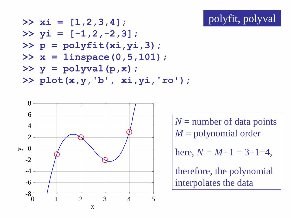
y>> xi = [1,2,3,4];
>> yi = [-1,2,-2,3];
>> p = polyfit(xi,yi,3);
>> x = linspace(0,5,101);
>> y = polyval(p,x);
>> plot(x,y,'b', xi,yi,'ro');
polyfit, polyval
N = number of data points
M = polynomial order
here, N = M+1 = 3+1=4,
therefore, the polynomial
interpolates the data

xi = [1, 3, 4, 6, 9];
yi = [4, 4, 7, 11, 19];
x = linspace(0,10,101);
for M = [1,2,3,4]
p = polyfit(xi,yi,M)
y = polyval(p,x);
figure;
plot(x,y,'r-', xi,yi,'b.', 'markersize',25);
yaxis(-2,22,0:5:20); xaxis(0,10,0:2:10);
xlabel('x'); title('polynomial fit');
legend([' fit, {\itM} = ',num2str(M)],...
' data', 'location','se');
end
polyfit, polyval

0 2 4 6 8 10
0
5
10
15
20
x
polynomial fit
fit , M = 1
da ta
0 2 4 6 8 10
0
5
10
15
20
x
polynomial fit
fit , M = 2
da ta
0 2 4 6 8 10
0
5
10
15
20
x
polynomial fit
fit , M = 3
da ta
0 2 4 6 8 10
0
5
10
15
20
x
polynomial fit
fit , M = 4
da ta

0 2 4 6 8 10 12 14 16 18 200
100
200
300
400
500
600
700
800
t
tota
ls
Ha nk Aa ron's H ome Run Output
linear fit
da ta
0 2 4 6 8 10 12 14 16 18 200
100
200
300
400
500
600
700
800
t
tota
ls
Ha nk Aa ron's H ome Run Output
y = 37x-37
da ta
% year ti H
% ---------------
1954 1 13
1955 2 27
1956 3 26
1957 4 44
1958 5 30
1959 6 39
1960 7 40
1961 8 34
1962 9 45
1963 10 44
1964 11 24
1965 12 32
1966 13 44
1967 14 39
1968 15 29
1969 16 44
1970 17 38
1971 18 47
1972 19 34
1973 20 40
aaron.dat

A = load('aaron.dat');
ti = A(:,2); H = A(:,3);
yi = cumsum(H);
p = polyfit(ti,yi,1)
% p =
% 37.2617 -39.8474
t = linspace(1,20, 101);
y = polyval(p,t);
plot(t,y,'r-', ...
ti,yi,'b.', ...
'markersize', 18);
0 2 4 6 8 10 12 14 16 18 200
100
200
300
400
500
600
700
800
t
tota
ls
Ha nk Aa ron's H ome Run Output
linear fit
da ta
0 2 4 6 8 10 12 14 16 18 200
100
200
300
400
500
600
700
800
t
tota
ls
Ha nk Aa ron's H ome Run Output
y = 37x-37
da ta

Given N data points {xi, yi}, i=1,2,…,N, the following data
models can be reduced to linear fits using an appropriate
transformation of the data:
p = polyfit(xi,log(yi),1); % exponential
y = exp(polyval(p,x)); % y=exp(a*x+log(b))
a = p(1); % y = exp(p(1)*x+p(2))
b = exp(p(2)); % so that y = b*exp(a*x)
1970 1980 1990 2000 201010
2
104
106
108
1010
year
cou
nt
t ra nsistor count
fit
da ta
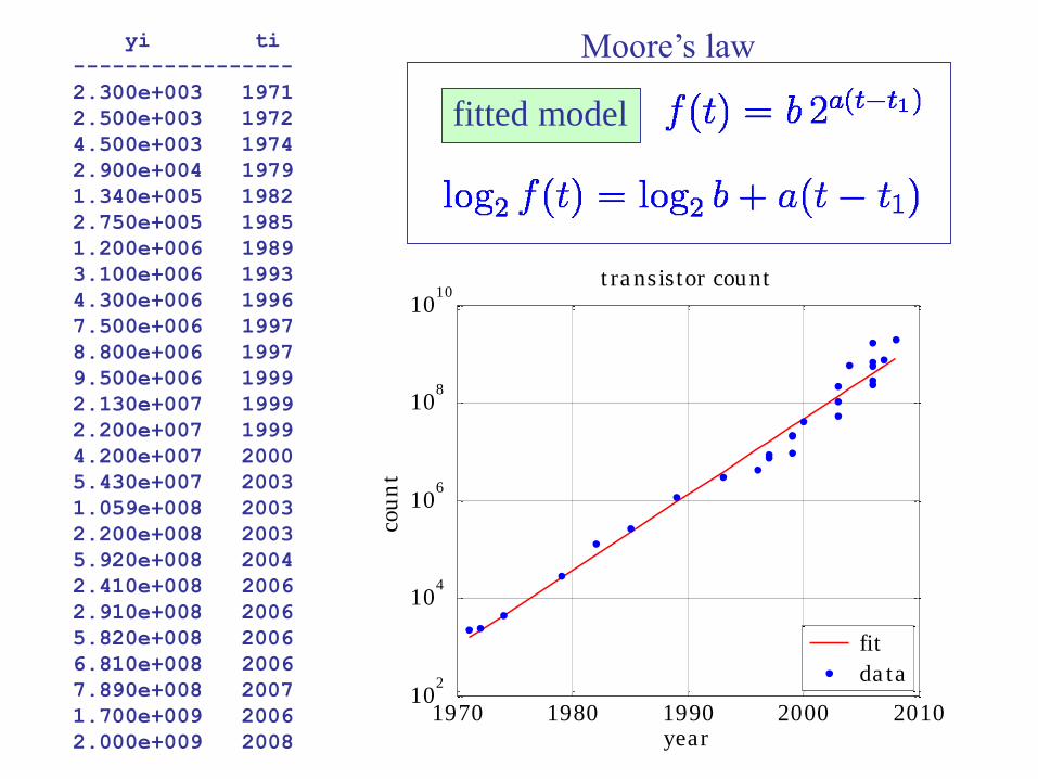
yi ti
-----------------
2.300e+003 1971
2.500e+003 1972
4.500e+003 1974
2.900e+004 1979
1.340e+005 1982
2.750e+005 1985
1.200e+006 1989
3.100e+006 1993
4.300e+006 1996
7.500e+006 1997
8.800e+006 1997
9.500e+006 1999
2.130e+007 1999
2.200e+007 1999
4.200e+007 2000
5.430e+007 2003
1.059e+008 2003
2.200e+008 2003
5.920e+008 2004
2.410e+008 2006
2.910e+008 2006
5.820e+008 2006
6.810e+008 2006
7.890e+008 2007
1.700e+009 2006
2.000e+009 2008
fitted model
Moore’s law

Y = load('transistor_count.dat');
y = Y(:,1); t = Y(:,2);
t1 = t(1); % t1 = 1971
p = polyfit(t-t1, log2(y), 1);
% p =
% 0.5138 10.5889 % b = 2^p(2) = 1.5402e+003
f = 2.^(polyval(p,t-t1));
semilogy(t,f,'r-', t,y,'b.', 'markersize',18)
fitted model:
f(t) = b * 2.^(a*(t-t1)) = 2.^(a*(t-t1)+log2(b));
% a = p(1), log2(b) = p(2) --> b = 2^(p(2))

1800 1840 1880 1920 1960 20001
2
3
4
5
6
t
log
(pop
)
US P opula t ion
quadra t ic fit
da ta
1800 1840 1880 1920 1960 20000
100
200
300
400
t
po
pu
lati
on
, m
illi
on
s
US P opula t ion
fit
da ta
% source: Wikipedia
% US population in millions
%
% ti yi
% ---------------
1790 3.929
1800 5.237
1810 7.240
1820 9.638
1830 12.866
1840 17.069
1850 23.192
1860 31.443
1870 38.558
1880 49.371
1890 62.980
1900 76.212
1910 92.229
1920 106.022
1930 123.202
1940 132.165
1950 151.326
1960 179.323
1970 203.212
1980 226.546
1990 248.710
2000 281.422
2010 308.746

A = load('uspop.dat');
ti = A(:,1); yi = A(:,2);
p = polyfit(ti,log(yi),2) % quadratic fit
% p =
% -0.0001 0.2653 -266.4672
t = linspace(1790, 2010, 201);
y = exp(polyval(p,t));
figure; plot(t, log(y), 'r-', ...
ti,log(yi),'b.','markersize',18);
figure; plot(t, y,'r-', ...
ti,yi,'b.','markersize',18);

planet ri Ti T_est
-----------------------------
Mercury 0.390 452 468
Earth 1.000 285 283
Mars 1.520 230 227
Jupiter 5.200 120 118
Saturn 9.539 88 85
Uranus 19.180 59 59
Neptune 30.060 48 46
Pluto 39.530 37 40
assumed model
Planetary Temperatures
Reference: M. C. LoPresto and N. Hagoort, "Determining Planetary Temperatures with the
Stefan-Boltzmann Law," Phys. Teacher, vol.49, 113 (2011). On sakai.
transformed model

ri = [0.39, 1, 1.52, 5.2, 9.539, 19.18, 30.06, 39.53]';
Ti = [452, 285, 230, 120, 88, 59, 48, 37]'; % columns
p = polyfit(log(ri),log(Ti),1)
c(2)=-p(1); c(1)=exp(p(2));
f = @(c,r) c(1)./r.^c(2);
r = linspace(0.35, 40, 100);
T = f(c,r);
T_est = f(c,ri);
plot(r,T,'r-', ri,Ti,'b.')
% c0 = [200;1]';
% c = nlinfit(ri,Ti,f,c0)
% c = [280.78; 0.5130]
% nlinfit version0 10 20 30 40
0
100
200
300
400
500
dista nce in AU, r
T
(K)
ba sis funct ions
da ta
estimated:
a = c(1) = 283.48
b = c(2) = 0.5329
% basis functions method
c = [ri.^0, -log(ri)] \ log(Ti);
c(1) = exp(c(1));

The curve fitting toolbox allows more complicated nonlinear
data fits. See also the statistics and optimization toolboxes.
>> doc curvefit % curve fitting toolbox
>> doc nlinfit % in statistics toolbox
>> doc lsqcurvefit % in optimization toolbox
c = nlinfit(xi,yi,f,c0);
% c = estimated parameter vector
% xi,yi = vectors of data points
% f = handle to fitting function y = f(c,x)
% c0 = initial parameter vector
% c = lsqcurvefit(f,c0,xi,yi);
c must be first
must be vectorized

An equivalent, do-it-yourself, least-squares version,
uses the built-in function fminsearch,
to mininize the least-squares error criterion:
J = @(c) sum((yi-f(c,xi)).^2); % L2 norm
c = fminsearch(J,c0);
% one can incorporate a weight vector wi
% J = @(c) sum(wi.*(yi-f(c,xi)).^2)
% one can also use the L1-norm criterion,
% which is generally more appropriate if
% there are outliers in the data
J = @(c) sum(abs(yi-f(c,xi))); % L1 norm
c = fminsearch(J,c0);
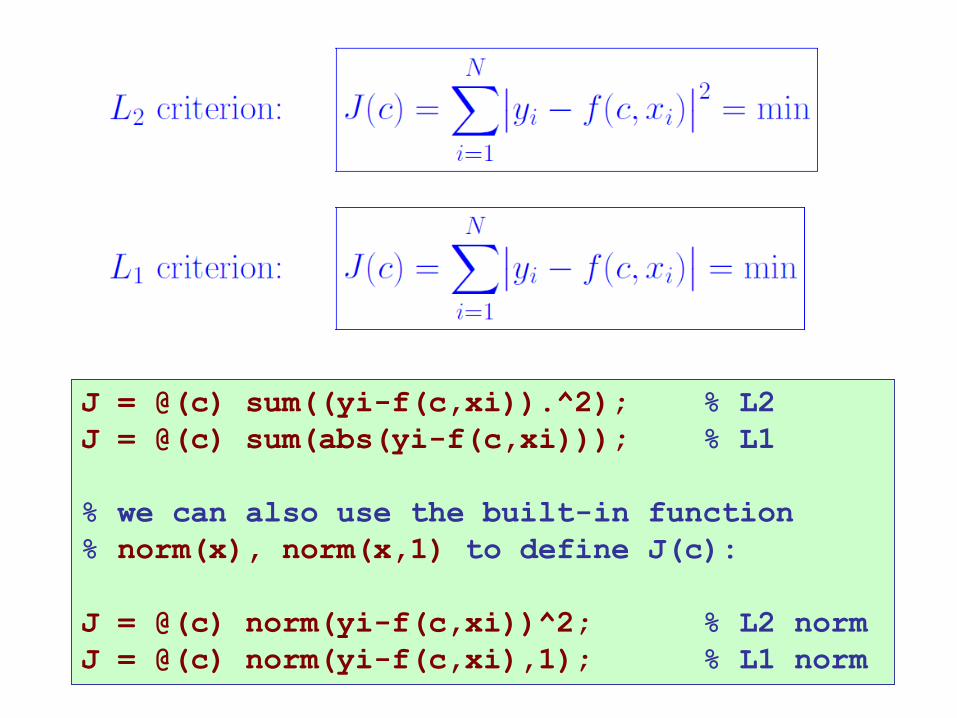
J = @(c) sum((yi-f(c,xi)).^2); % L2
J = @(c) sum(abs(yi-f(c,xi))); % L1
% we can also use the built-in function
% norm(x), norm(x,1) to define J(c):
J = @(c) norm(yi-f(c,xi))^2; % L2 norm
J = @(c) norm(yi-f(c,xi),1); % L1 norm

>> doc curvefit % curve fitting toolbox
% see also
>> doc nlinfit % in statistics toolbox
>> doc lsqcurvefit % in optimization toolbox
>> doc lsqnonlin % nonlinear least-squares
>> doc lsqlin % linear with constraints
>> doc linprog % linear programming
>> doc lsqnonneg % positivity contraints
>> doc quadprog % quadratic programming
>> doc bintprog % binary int programming
useful built-in MATLAB functions

nlinfit Example 1:
f = @(c,t) c(1) + c(2)*cos(c(3)*t).*exp(-c(4)*t);
ce = [1 2 15 1]'; % c = [c1,c2,c3,c4]' = column
rng(201);
ti = 0:0.1:2.9;
yi = f(ce,ti) + 0.2*randn(size(ti));
c0 = [10 10 10 10]';
c = nlinfit(ti,yi,f,c0);
% c = lsqcurvefit(f,c0,ti,yi); [c,be] =
0.9999 1
1.8271 2
15.0056 15
0.9238 1
estimated parameter vector
initial guess
noisy data
parameter vector c = [c1, c2, c3, c4]'
exact model

0 1 2 3-1
0
1
2
3
4
t
fit ted
exact
da ta
t = linspace(0,3,301);
plot(t,f(c,t),'r-', t,f(ce,t),'b:', ti,yi,'b.')
fitted exact data

nlinfit Example 2: Cosmic Microwave Background (CMB)
In 1964 Penzias and Wilson discovered the cosmic blackbody thermal
radiation background, a remnant of the Big Bang, that almost uniformly
fills the entire universe, and predicted theoretically in 1948 by Gamow, Alpher and Herman.
source: http://aether.lbl.gov/www/projects/cobe/cobe_pics.html
NASA's Cosmic Background
Explorer (COBE) satellite,
launched in 1989, carried out
very accurate measurements of
the CMB frequency spectrum
using a Far-Infrared Absolute
Spectrophotometer (FIRAS).
The measurements provided an
almost perfect fit to Planck's
blackbody spectrum at a temperature of T = 2.7250 K

Planck's blackbody radiation formulas
spectral radiance

Least-squares method
Least-squares error criterion:
find T that minimizes E(T)
using fminbnd or nlinfit
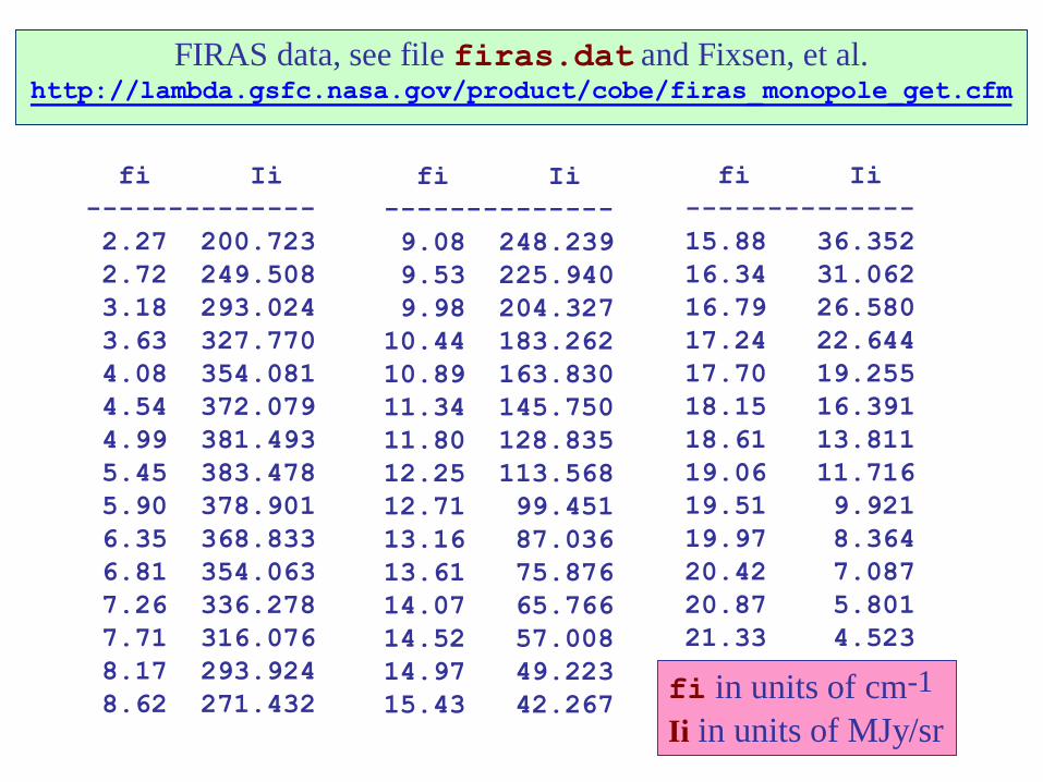
fi Ii
--------------
2.27 200.723
2.72 249.508
3.18 293.024
3.63 327.770
4.08 354.081
4.54 372.079
4.99 381.493
5.45 383.478
5.90 378.901
6.35 368.833
6.81 354.063
7.26 336.278
7.71 316.076
8.17 293.924
8.62 271.432
fi Ii
--------------
9.08 248.239
9.53 225.940
9.98 204.327
10.44 183.262
10.89 163.830
11.34 145.750
11.80 128.835
12.25 113.568
12.71 99.451
13.16 87.036
13.61 75.876
14.07 65.766
14.52 57.008
14.97 49.223
15.43 42.267
fi Ii
--------------
15.88 36.352
16.34 31.062
16.79 26.580
17.24 22.644
17.70 19.255
18.15 16.391
18.61 13.811
19.06 11.716
19.51 9.921
19.97 8.364
20.42 7.087
20.87 5.801
21.33 4.523
FIRAS data, see file firas.dat and Fixsen, et al.http://lambda.gsfc.nasa.gov/product/cobe/firas_monopole_get.cfm
fi in units of cm-1
Ii in units of MJy/sr

h = 6.62606957e-34; % J/Hz, Planck's constant
c = 2.99792458e8; % m/s, speed of light
k = 1.3806488e-23; % J/K, Boltzmann constant
A = 10^47 * 2*h/c^2; % A = 0.00147450
B = 10^9 * h/k; % B = 0.04799243
Y = load('firas.dat'); % load COBE data
fi = Y(:,1) * c * 1e-7; % convert fi to GHz
Ii = Y(:,2); % Ii in MJy/sr
I = @(T,f) A*f.^3./(exp(B*f/T) - 1);
T = nlinfit(fi,Ii,I,3); % T = 2.725013 K
% implement our own least-squares method
E = @(T) sum((Ii - I(T,fi)).^2);
T = fminbnd(E,1,3); % T = 2.725015 K
vectorized in f
sum of squared errors

f = linspace(50,690,641);
If = I(T,f);
plot(f,If,'r-', fi,Ii,'b.');
0 100 200 300 400 500 600 7000
100
200
300
400
f (GH z)
rad
ian
ce (
MJ
y/s
r)
CMB spect rum, wit h T = 2.7250 K
Planck spect rum
da ta
CMB data provide a
remarkable confirmation
of quantum theory

nlinfit Example 3:
% generate simulated data
A = 5; B = 1; a = 2;
rng(100);
ti = 0:0.3:3;
yi = (A*ti+B).*exp(-a*ti) + ...
0.05*randn(size(ti));
yi = round(yi*100)/100;
ce = [A,B,a]';
c0 = [1 1 1]';
% define nlinfit model function
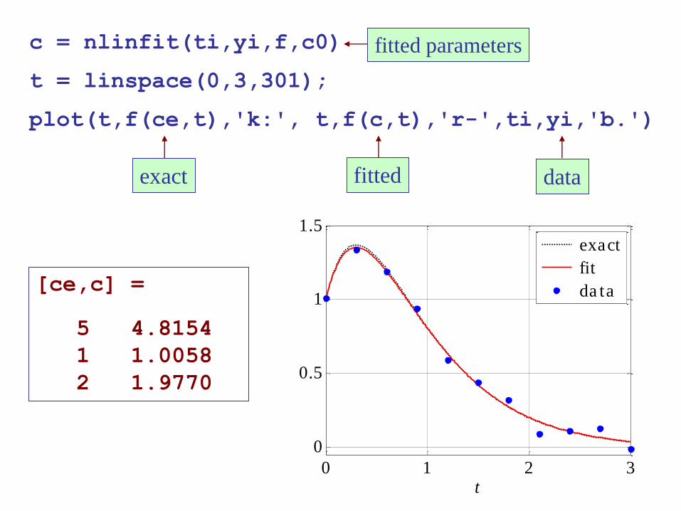
f = @(c,t) (c(1)*t+c(2)).*exp(-c(3)*t);
ti yi
----------
0.0 1.01
0.3 1.34
0.6 1.19
0.9 0.94
1.2 0.59
1.5 0.44
1.8 0.32
2.1 0.09
2.4 0.11
2.7 0.13
3.0 -0.01
assumed model
exact values
exact parameters
initial parameters
fittedexact data
c = nlinfit(ti,yi,f,c0)
t = linspace(0,3,301);
plot(t,f(ce,t),'k:', t,f(c,t),'r-',ti,yi,'b.')
[ce,c] =
5 4.8154
1 1.0058
2 1.9770
fitted parameters
0 1 2 3
0
0.5
1
1.5
t
exact
fit
da ta

nlinfit Example 4: Logistic function
t0 t0
t
f t( ) df t dt( )/
t
K rK/4 = maximum
K/2 inflection point

ti
-----
1.1
2.9
4.5
7.5
9.0
10.5
12.9
15.3
17.4
initial parameters
f = @(c,t) c(1)./ (1 + exp(-c(2)*(t-c(3))));
[df0,i0] = max(diff(yi)./diff(ti));
K0 = max(yi);
r0 = 4*df0/K0;
t0 = ti(i0);
c0 = [K0, r0, t0]';
c = nlinfit(ti,yi,f,c0);
K = c(1); r = c(2); t0 = c(3);
% data inluded in file logsim.m
fitted
data
define logistic
function of the three
parameters K, r, t0
initial estimatesyi
----
0.04
1.13
1.22
3.87
5.33
6.51
8.37
8.67
9.03

fitted data
t = linspace(0,18,181);
plot(t,f(c,t), 'b-', ti,yi,'r.', t0,K/2,'g.');
inflection point
0 2 4 6 8 10 12 14 16 18
0
2
4
6
8
10
12
K = 9.1672, r = 0.4496, t0 = 8.2870
t
f(t)
f (t) =K
1 + e! r (t ! t0)
model, f(t)
da ta
in flect ion, t0 see M-file
logsim.m
on sakai, week-11

ti yi
-----------
1.1 0.04
2.9 1.13
4.5 1.22
7.5 3.87
9.0 5.33
10.5 6.51
12.9 11.00
15.3 8.67
17.4 9.03
% use the same definitions of
% f(c,t), c0, and t
J = @(c) sum(abs(yi - f(c,ti)));
c1 = fminsearch(J,c0); % L1
J = @(c) sum((yi - f(c,ti)).^2);
c2 = fminsearch(J,c0); % L2
plot(t,f(c1,t), 'b-',...
t,f(c2,t), 'b--',...
ti,yi,'r.');
data
outlier
compare the L1 and L2 criteria when
there are outliers in the data

0 2 4 6 8 10 12 14 16 18
0
2
4
6
8
10
12
compar ison of L1 and L
2 cr iteria
t
f(t)
f (t) =K
1 + e! r (t ! t0)
out lier ! L1
L2
da ta

Variety of Growth Models