Introduction to Analysis in One Variable Michael Taylor
288
Introduction to Analysis in One Variable Michael Taylor Math. Dept., UNC E-mail address : [email protected]
Transcript of Introduction to Analysis in One Variable Michael Taylor

Introduction to Analysis in One Variable
Michael Taylor
Math. Dept., UNC
E-mail address: [email protected]

2010 Mathematics Subject Classification. 26A03, 26A06, 26A09, 26A42
Key words and phrases. real numbers, complex numbers, irrationalnumbers, Euclidean space, metric spaces, compact spaces, Cauchysequences, continuous function, power series, derivative, mean value
theorem, Riemann integral, fundamental theorem of calculus, arclength,exponential function, logarithm, trigonometric functions, Euler’s formula,Weierstrass approximation theorem, Fourier series, Newton’s method

Contents
Preface ix
Some basic notation xiii
Chapter 1. Numbers 1
§1.1. Peano arithmetic 2
§1.2. The integers 9
§1.3. Prime factorization and the fundamental theorem of arithmetic 14
§1.4. The rational numbers 16
§1.5. Sequences 21
§1.6. The real numbers 29
§1.7. Irrational numbers 41
§1.8. Cardinal numbers 44
§1.9. Metric properties of R 51
§1.10. Complex numbers 56
Chapter 2. Spaces 65
§2.1. Euclidean spaces 66
§2.2. Metric spaces 74
§2.3. Compactness 80
§2.4. The Baire category theorem 85
Chapter 3. Functions 87
§3.1. Continuous functions 88
§3.2. Sequences and series of functions 97
vii
viii Contents
§3.3. Power series 102
§3.4. Spaces of functions 108
§3.5. Absolutely convergent series 112
Chapter 4. Calculus 117
§4.1. The derivative 119
§4.2. The integral 129
§4.3. Power series 148
§4.4. Curves and arc length 158
§4.5. The exponential and trigonometric functions 172
§4.6. Unbounded integrable functions 191
Chapter 5. Further Topics in Analysis 199
§5.1. Convolutions and bump functions 200
§5.2. The Weierstrass approximation theorem 205
§5.3. The Stone-Weierstrass theorem 208
§5.4. Fourier series 212
§5.5. Newton’s method 237
§5.6. Inner product spaces 243
Appendix A. Complementary results 247
§A.1. The fundamental theorem of algebra 247
§A.2. More on the power series of (1− x)b 249
§A.3. π2 is irrational 251
§A.4. Archimedes’ approximation to π 253
§A.5. Computing π using arctangents 257
§A.6. Power series for tanx 261
§A.7. Abel’s power series theorem 264
§A.8. Continuous but nowhere-differentiable functions 268
Bibliography 273
Index 275
Preface
This is a text for students who have had a three course calculus sequence,and who are ready for a course that explores the logical structure of thisarea of mathematics, which forms the backbone of analysis. This is intendedfor a one semester course. An accompanying text, Introduction to Analysisin Several Variables [13], can be used in the second semester of a one yearsequence.
The main goal of Chapter 1 is to develop the real number system. Westart with a treatment of the “natural numbers” N, obtaining its structurefrom a short list of axioms, the primary one being the principle of induction.Then we construct the set Z of all integers, which has a richer algebraicstructure, and proceed to construct the set Q of rational numbers, whichare quotients of integers (with a nonzero denominator). After discussinginfinite sequences of rational numbers, including the notions of convergentsequences and Cauchy sequences, we construct the set R of real numbers,as ideal limits of Cauchy sequences of rational numbers. At the heart ofthis chapter is the proof that R is complete, i.e., Cauchy sequences of realnumbers always converge to a limit in R. This provides the key to studyingother metric properties of R, such as the compactness of (nonempty) closed,bounded subsets. We end Chapter 1 with a section on the set C of complexnumbers. Many introductions to analysis shy away from the use of complexnumbers. My feeling is that this forecloses the study of way too manybeautiful results that can be appreciated at this level. This is not a coursein complex analysis. That is for another course, and with another text (suchas [14]). However, I think the use of complex numbers in this text servesboth to simplify the treatment of a number of key concepts, and to extendtheir scope in natural and useful ways.
ix
x Preface
In fact, the structure of analysis is revealed more clearly by movingbeyond R and C, and we undertake this in Chapter 2. We start with atreatment of n-dimensional Euclidean space, Rn. There is a notion of Eu-clidean distance between two points in Rn, leading to notions of convergenceand of Cauchy sequences. The spaces Rn are all complete, and again closedbounded sets are compact. Going through this sets one up to appreciate afurther generalization, the notion of a metric space, introduced in §2.2. Thisis followed by §2.3, exploring the notion of compactness in a metric spacesetting.
Chapter 3 deals with functions. It starts in a general setting, of func-tions from one metric space to another. We then treat infinite sequencesof functions, and study the notion of convergence, particularly of uniformconvergence of a sequence of functions. We move on to infinite series. Insuch a case, we take the target space to be Rn, so we can add functions.Section 3.3 treats power series. Here, we study series of the form
(0.0.1)∞∑k=0
ak(z − z0)k,
with ak ∈ C and z running over a disk in C. For results obtained in thissection, regarding the radius of convergence R and the continuity of the sumon DR(z0) = z ∈ C : |z−z0| < R, there is no extra difficulty in allowing akand z to be complex, rather than insisting they be real, and the extra levelof generality will pay big dividends in Chapter 4. One section in Chapter 3is devoted to spaces of functions, illustrating the utility of studying spacesbeyond the case of Rn.
Chapter 4 gets to the heart of the matter, a rigorous development of dif-ferential and integral calculus. We define the derivative in §4.1, and provethe Mean Value Theorem, making essential use of compactness of a closed,bounded interval and its consequences, established in earlier chapters. Thisresult has many important consequences, such as the Inverse Function The-orem, and especially the Fundamental Theorem of Calculus, established in§4.2, after the Riemann integral is introduced. In §4.3, we return to powerseries, this time of the form
(0.0.2)∞∑k=0
ak(t− t0)k.
We require t and t0 to be in R, but still allow ak ∈ C. Results on radiusof convergence R and continuity of the sum f(t) on (t0 − R, t0 + R) followfrom material in Chapter 3. The essential new result in §4.3 is that one canobtain the derivative f ′(t) by differentiating the power series for f(t) termby term. In §4.4 we consider curves in Rn, and obtain a formula for arclength for a smooth curve. We show that a smooth curve with nonvanishing
Preface xi
velocity can be parametrized by arc length. When this is applied to the unitcircle in R2 centered at the origin, one is looking at the standard definitionof the trigonometric functions,
(0.0.3) C(t) = (cos t, sin t).
We provide a demonstration that
(0.0.4) C ′(t) = (− sin t, cos t)
that is much shorter than what is usually presented in calculus texts. In§4.5 we move on to exponential functions. We derive the power series forthe function et, introduced to solve the differential equation dx/dt = x. Wethen observe that with no extra work we get an analogous power series foreat, with derivative aeat, and that this works for complex a as well as forreal a. It is a short step to realize that eit is a unit speed curve tracing outthe unit circle in C ≈ R2, so comparison with (0.0.3) gives Euler’s formula
(0.0.5) eit = cos t+ i sin t.
That the derivative of eit is ieit provides a second proof of (0.0.4). Thuswe have a unified treatment of the exponential and trigonometric functions,carried out further in §4.5, with details developed in numerous exercises.Section 4.6 extends the scope of the Riemann integral to a class of unboundedfunctions.
Chapter 5 treats further topics in analysis. The topics center aroundapproximating functions, via various infinite sequences or series. Topicsinclude polynomial approximation of continuous functions, Fourier series,and Newton’s method for approximating the inverse of a given function.
We end with a collection of appendices, covering various results relatedto material in Chapters 4–5. The first one gives a proof of the fundamentaltheorem of algebra, that every nonconstant polynomial has a complex root.The second explores the power series of (1− x)b, in more detail then domein §4.3, of use in §5.2. There follow three appendices on the nature of π andits numerical evaluation, an appendix on the power series of tanx, and oneon a theorem of Abel on infinite series, and related results. We also studycontinuous functions on R that are nowhere differentiable.
Our approach to the foundations of analysis, outlined above, has somedistinctive features, which we point out here.
1) Approach to numbers. We do not take an axiomatic approach to thepresentation of the real numbers. Rather than hypothesizing that R hasspecified algebraic and metric properties, we build R from more basic objects
xii Preface
(natural numbers, integers, rational numbers) and produce results on itsalgebraic and metric properties as propositions, rather than as axioms.
In addition, we do not shy away from the use of complex numbers. Thesimplifications this use affords range from amusing (construction of a regularpentagon) to profound (Euler’s identity, computing the Dirichlet kernel inFourier series), and such uses of complex numbers can be readily appreciatedby a student at the level of this sort of analysis course.
2) Spaces and geometrical concepts. We emphasize the use of geometricalproperties of n-dimensional Euclidean space, Rn, as an important extensionof metric properties of the line and the plane. Going further, we introducethe notion of metric spaces early on, as a natural extension of the class ofEuclidean spaces. For one interested in functions of one real variable, it isvery useful to encounter such functions taking values in Rn (i.e., curves),and to encounter spaces of functions of one variable (a significant class ofmetric spaces).
One implementation of this approach involves defining the exponentialfunction for complex arguments and making a direct geometrical study ofeit, for real t. This allows for a self-contained treatment of the trigonomet-ric functions, not relying on how this topic might have been covered in aprevious course, and in particular for a derivation of the Euler identity thatis very much different from what one typically sees.
We follow this introduction with a record of some standard notation thatwill be used throughout this text.
AcknowledgmentDuring the preparation of this book, I have been supported by a number ofNSF grants, most recently DMS-1500817.
Some basic notation
R is the set of real numbers.
C is the set of complex numbers.
Z is the set of integers.
Z+ is the set of integers ≥ 0.
N is the set of integers ≥ 1 (the “natural numbers”).
Q is the set of rational numbers.
x ∈ R means x is an element of R, i.e., x is a real number.
(a, b) denotes the set of x ∈ R such that a < x < b.
[a, b] denotes the set of x ∈ R such that a ≤ x ≤ b.
x ∈ R : a ≤ x ≤ b denotes the set of x in R such that a ≤ x ≤ b.
[a, b) = x ∈ R : a ≤ x < b and (a, b] = x ∈ R : a < x ≤ b.
xiii

xiv Some basic notation
z = x− iy if z = x+ iy ∈ C, x, y ∈ R.
Ω denotes the closure of the set Ω.
f : A→ B denotes that the function f takes points in the set A to pointsin B. One also says f maps A to B.
x→ x0 means the variable x tends to the limit x0.
f(x) = O(x) means f(x)/x is bounded. Similarly g(ε) = O(εk) meansg(ε)/εk is bounded.
f(x) = o(x) as x→ 0 (resp., x→ ∞) means f(x)/x→ 0 as x tends to thespecified limit.
S = supn
|an| means S is the smallest real number that satisfies S ≥ |an| forall n. If there is no such real number then we take S = +∞.
lim supk→∞
|ak| = limn→∞
(supk≥n
|ak|).
Chapter 1
Numbers
One foundation for a course in analysis is a solid understanding of the realnumber system. Texts vary on just how to achieve this. Some take an ax-iomatic approach. In such an approach, the set of real numbers is hypothe-sized to have a number of properties, including various algebraic propertiessatisfied by addition and multiplication, order axioms, and, crucially, thecompleteness property, sometimes expressed as the supremum property.
This is not the approach we will take. Rather, we will start with a smalllist of axioms for the natural numbers (i.e., the positive integers), and thenbuild the rest of the edifice logically, obtaining the basic properties of thereal number system, particularly the completeness property, as theorems.
Sections 1.1–1.3 deal with the integers, starting in §1.1 with the set Nof natural numbers. The development proceeds from axioms of G. Peano.The main one is the principle of mathematical induction. We deduce basicresults about integer arithmetic from these axioms. A high point is thefundamental theorem of arithmetic, presented in §1.3.
Section 1.4 discusses the set Q of rational numbers, deriving the basicalgebraic properties of these numbers from the results of §§1.1–1.3. Section1.5 provides a bridge between §1.4 and §1.6. It deals with infinite sequences,including convergent sequences and “Cauchy sequences.”
This prepares the way for §1.6, the main section of this chapter. Here weconstruct the set R of real numbers, as “ideal limits” of rational numbers.We extend basic algebraic results fromQ to R. Furthermore, we establish theresult that R is “complete,” i.e., Cauchy sequences always have limits in R.Section 1.7 provides examples of irrational numbers, such as
√2,√3,√5,...
1
2 1. Numbers
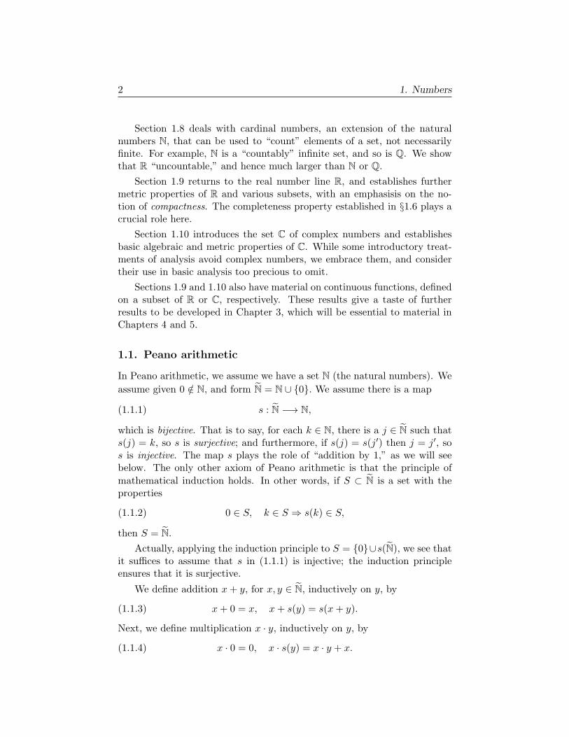
Section 1.8 deals with cardinal numbers, an extension of the naturalnumbers N, that can be used to “count” elements of a set, not necessarilyfinite. For example, N is a “countably” infinite set, and so is Q. We showthat R “uncountable,” and hence much larger than N or Q.
Section 1.9 returns to the real number line R, and establishes furthermetric properties of R and various subsets, with an emphasisis on the no-tion of compactness. The completeness property established in §1.6 plays acrucial role here.
Section 1.10 introduces the set C of complex numbers and establishesbasic algebraic and metric properties of C. While some introductory treat-ments of analysis avoid complex numbers, we embrace them, and considertheir use in basic analysis too precious to omit.
Sections 1.9 and 1.10 also have material on continuous functions, definedon a subset of R or C, respectively. These results give a taste of furtherresults to be developed in Chapter 3, which will be essential to material inChapters 4 and 5.
1.1. Peano arithmetic
In Peano arithmetic, we assume we have a set N (the natural numbers). We
assume given 0 /∈ N, and form N = N ∪ 0. We assume there is a map
(1.1.1) s : N −→ N,
which is bijective. That is to say, for each k ∈ N, there is a j ∈ N such thats(j) = k, so s is surjective; and furthermore, if s(j) = s(j′) then j = j′, sos is injective. The map s plays the role of “addition by 1,” as we will seebelow. The only other axiom of Peano arithmetic is that the principle of
mathematical induction holds. In other words, if S ⊂ N is a set with theproperties
(1.1.2) 0 ∈ S, k ∈ S ⇒ s(k) ∈ S,
then S = N.Actually, applying the induction principle to S = 0∪s(N), we see that
it suffices to assume that s in (1.1.1) is injective; the induction principleensures that it is surjective.
We define addition x+ y, for x, y ∈ N, inductively on y, by
(1.1.3) x+ 0 = x, x+ s(y) = s(x+ y).
Next, we define multiplication x · y, inductively on y, by
(1.1.4) x · 0 = 0, x · s(y) = x · y + x.
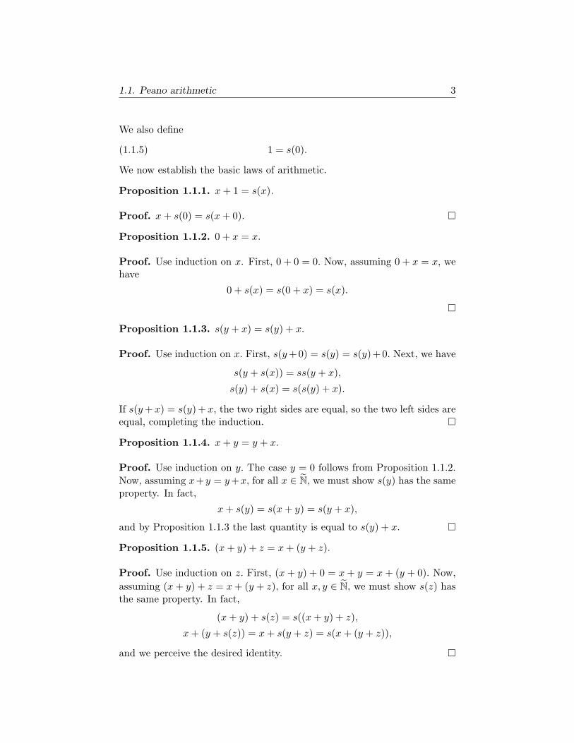
1.1. Peano arithmetic 3
We also define
(1.1.5) 1 = s(0).
We now establish the basic laws of arithmetic.
Proposition 1.1.1. x+ 1 = s(x).
Proof. x+ s(0) = s(x+ 0).
Proposition 1.1.2. 0 + x = x.
Proof. Use induction on x. First, 0 + 0 = 0. Now, assuming 0 + x = x, wehave
0 + s(x) = s(0 + x) = s(x).
Proposition 1.1.3. s(y + x) = s(y) + x.
Proof. Use induction on x. First, s(y+0) = s(y) = s(y)+0. Next, we have
s(y + s(x)) = ss(y + x),
s(y) + s(x) = s(s(y) + x).
If s(y+x) = s(y)+x, the two right sides are equal, so the two left sides areequal, completing the induction.
Proposition 1.1.4. x+ y = y + x.
Proof. Use induction on y. The case y = 0 follows from Proposition 1.1.2.
Now, assuming x+y = y+x, for all x ∈ N, we must show s(y) has the sameproperty. In fact,
x+ s(y) = s(x+ y) = s(y + x),
and by Proposition 1.1.3 the last quantity is equal to s(y) + x.
Proposition 1.1.5. (x+ y) + z = x+ (y + z).
Proof. Use induction on z. First, (x+ y) + 0 = x+ y = x+ (y + 0). Now,
assuming (x+ y) + z = x+ (y + z), for all x, y ∈ N, we must show s(z) hasthe same property. In fact,
(x+ y) + s(z) = s((x+ y) + z),
x+ (y + s(z)) = x+ s(y + z) = s(x+ (y + z)),
and we perceive the desired identity.
4 1. Numbers
Remark. Propositions 1.1.4 and 1.1.5 state the commutative and associa-tive laws for addition.
We now establish some laws for multiplication.
Proposition 1.1.6. x · 1 = x.
Proof. We have
x · s(0) = x · 0 + x = 0 + x = x,
the last identity by Proposition 1.1.2.
Proposition 1.1.7. 0 · y = 0.
Proof. Use induction on y. First, 0 · 0 = 0. Next, assuming 0 · y = 0, wehave 0 · s(y) = 0 · y + 0 = 0 + 0 = 0.
Proposition 1.1.8. s(x) · y = x · y + y.
Proof. Use induction on y. First, s(x) · 0 = 0, while x · 0 + 0 = 0 + 0 = 0.Next, assuming s(x) · y = x · y + y, for all x, we must show that s(y) hasthis property. In fact,
s(x) · s(y) = s(x) · y + s(x) = (x · y + y) + (x+ 1),
x · s(y) + s(y) = (x · y + x) + (y + 1),
and identity then follows via the commutative and associative laws of addi-tion, Propositions 1.1.4 and 1.1.5.
Proposition 1.1.9. x · y = y · x.
Proof. Use induction on y. First, x · 0 = 0 = 0 · x, the latter identity by
Proposition 1.1.7. Next, assuming x · y = y · x for all x ∈ N, we must showthat s(y) has the same property. In fact,
x · s(y) = x · y + x = y · x+ x,
s(y) · x = y · x+ x,
the last identity by Proposition 1.1.8.
Proposition 1.1.10. (x+ y) · z = x · z + y · z.
Proof. Use induction on z. First, the identity clearly holds for z = 0. Next,
assuming it holds for z (for all x, y ∈ N), we must show it holds for s(z). Infact,
(x+ y) · s(z) = (x+ y) · z + (x+ y) = (x · z + y · z) + (x+ y),
x · s(z) + y · s(z) = (x · z + x) + (y · z + y),
1.1. Peano arithmetic 5
and the desired identity follows from the commutative and associative lawsof addition.
Proposition 1.1.11. (x · y) · z = x · (y · z).
Proof. Use induction on z. First, the identity clearly holds for z = 0. Next,
assuming it holds for z (for all x, y ∈ N), we have
(x · y) · s(z) = (x · y) · z + x · y,
while
x · (y · s(z)) = x · (y · z + y) = x · (y · z) + x · y,the last identity by Proposition 1.1.10 (and 1.1.9). These observations yieldthe desired identity.
Remark. Propositions 1.1.9 and 1.1.11 state the commutative and associa-tive laws for multiplication. Proposition 1.10 is the distributive law. Com-bined with Proposition 1.1.9, it also yields
z · (x+ y) = z · x+ z · y,
used above.
We next demonstrate the cancellation law of addition:
Proposition 1.1.12. Given x, y, z ∈ N,
(1.1.6) x+ y = z + y =⇒ x = z.
Proof. Use induction on y. If y = 0, (1.1.6) obviously holds. Assuming(1.1.6) holds for y, we must show that
(1.1.7) x+ s(y) = z + s(y)
implies x = z. In fact, (1.1.7) is equivalent to s(x+ y) = s(z + y). Since themap s is assumed to be one-to-one, this implies that x + y = z + y, so weare done.
We next define an order relation on N. Given x, y ∈ N, we say
(1.1.8) x < y ⇐⇒ y = x+ u, for some u ∈ N.
Similarly there is a definition of x ≤ y. We have x ≤ y if and only if y ∈ Rx,where
(1.1.9) Rx = x+ u : u ∈ N.
Other notation is
y > x⇐⇒ x < y, y ≥ x⇐⇒ x ≤ y.
6 1. Numbers
Proposition 1.1.13. If x ≤ y and y ≤ x then x = y.
Proof. The hypotheses imply
(1.1.10) y = x+ u, x = y + v, u, v ∈ N.
Hence x = x + u + v, so, by Proposition 1.1.12, u + v = 0. Now, if v = 0,then v = s(w), so u+ v = s(u+ w) ∈ N. Thus v = 0, and u = 0.
Proposition 1.1.14. Given x, y ∈ N, either
(1.1.11) x < y, or x = y, or y < x,
and no two can hold.
Proof. That no two of (1.1.11) can hold follows from Proposition 1.1.13. It
remains to show that one must hold. Take y ∈ N. We will establish (1.1.11)by induction on x. Clearly (1.1.11) holds for x = 0. We need to show that
if (1.1.11) holds for a given x ∈ N, then either
(1.1.12) s(x) < y, or s(x) = y, or y < s(x).
Consider the three possibilities in (1.1.11). If either y = x or y < x, thenclearly y < s(x) = x + 1. On the other hand, if x < y, we can use theimplication
(1.1.13) x < y =⇒ s(x) ≤ y
to complete the proof of (1.1.12). See Lemma 1.1.17 for a proof of (1.1.13).
We can now establish the cancellation law for multiplication.
Proposition 1.1.15. Given x, y, z ∈ N,
(1.1.14) x · y = x · z, x = 0 =⇒ y = z.
Proof. If y = z, then either y < z or z < y. Suppose y < z, i.e., z =y + u, u ∈ N. Then the hypotheses of (1.1.14) imply
x · y = x · y + x · u, x = 0,
hence, by Proposition 1.1.12,
(1.1.15) x · u = 0, x = 0.
We thus need to show that (1.1.15) implies u = 0. In fact, if not, then we
can write u = s(w), and x = s(a), with w, a ∈ N, and we have
(1.1.16) x · u = x · w + s(a) = s(x · w + a) ∈ N.
This contradicts (1.1.15), so we are done.
1.1. Peano arithmetic 7
Remark. Note that (1.1.16) implies
(1.1.17) x, y ∈ N =⇒ x · y ∈ N.
We next establish the following variant of the principle of induction,
called the well-ordering property of N.
Proposition 1.1.16. If T ⊂ N is nonempty, then T contains a smallestelement.
Proof. Suppose T contains no smallest element. Then 0 /∈ T. Let
(1.1.18) S = x ∈ N : x < y, ∀ y ∈ T.
Then 0 ∈ S. We claim that
(1.1.19) x ∈ S =⇒ s(x) ∈ S.
Indeed, suppose x ∈ S, so x < y for all y ∈ T. If s(x) /∈ S, we have s(x) ≥ y0for some y0 ∈ T. On the other hand (see Lemma 1.1.17 below),
(1.1.20) x < y0 =⇒ s(x) ≤ y0.
Thus, by Proposition 1.1.13,
(1.1.21) s(x) = y0.
It follows that y0 must be the smallest element of T. Thus, if T has nosmallest element, (1.1.19) must hold. The induction principle then implies
that S = N, which implies T is empty.
Here is the result behind (1.1.13) and (1.1.20).
Lemma 1.1.17. Given x, y ∈ N,
(1.1.22) x < y =⇒ s(x) ≤ y.
Proof. Indeed, x < y ⇒ y = x+ u with u ∈ N, hence u = s(v), so
y = x+ s(v) = s(x+ v) = s(x) + v,
hence s(x) ≤ y.
Remark. Proposition 1.1.16 has a converse, namely, the assertion
(1.1.23) T ⊂ N nonempty =⇒ T contains a smallest element
implies the principle of induction:
(1.1.24)(0 ∈ S ⊂ N, k ∈ S ⇒ s(k) ∈ S
)=⇒ S = N.

8 1. Numbers
To see this, suppose S satisfies the hypotheses of (1.1.24), and let T = N\S.If S = N, then T is nonempty, so (1.1.23) implies T has a smallest element,say x1. Since 0 ∈ S, x1 ∈ N, so x1 = s(x0), and we must have
(1.1.25) x0 ∈ S, s(x0) ∈ T = N \ S,contradicting the hypotheses of (1.1.24).
Exercises
Given n ∈ N, we define∑n
k=1 ak inductively, as follows.
(1.1.26)
1∑k=1
ak = a1,
n+1∑k=1
ak =( n∑k=1
ak
)+ an+1.
Use the principle of induction to establish the following identities.
1. Linear series
(1.1.27) 2
n∑k=1
k = n(n+ 1).
2. Quadratic series
(1.1.28) 6n∑
k=1
k2 = n(n+ 1)(2n+ 1).
3. Geometric series
(1.1.29) (a− 1)
n∑k=1
ak = an+1 − a, if a = 1.
Here, we define the powers an inductively by
(1.1.30) a1 = a, an+1 = an · a.
4. We also set a0 = 1 if a ∈ N, and∑n
k=0 ak = a0 +∑n
k=1 ak. Verify that
(1.1.31) (a− 1)
n∑k=0
ak = an+1 − 1, if a = 1.
5. Given k ∈ N, show that
2k ≥ 2k,
with strict inequality for k > 1.
1.2. The integers 9
6. Show that, for x, x′, y, y′ ∈ N,x < x′, y ≤ y′ =⇒ x+ y < x′ + y′, and
x · y < x′ · y′, if also y′ > 0.
7. Show that the following variant of the principle of induction holds:(1 ∈ S ⊂ N, k ∈ S ⇒ s(k) ∈ S
)=⇒ S = N.
Hint. Consider 0 ∪ S ⊂ N.More generally, with Rx as in (1.9), show that, for x ∈ N,(
x ∈ S ⊂ Rx, k ∈ S ⇒ s(k) ∈ S)=⇒ S = Rx.
Hint. Use induction on x.
8. With an defined inductively as in (1.1.30) for a ∈ N, n ∈ N, show that ifalso m ∈ N,
aman = am+n, (am)n = amn.
Hint. Use induction on n.
1.2. The integers
An integer is thought of as having the form x−a, with x, a ∈ N. To be moreformal, we will define an element of Z as an equivalence class of ordered
pairs (x, a), x, a ∈ N, where we define
(1.2.1) (x, a) ∼ (y, b) ⇐⇒ x+ b = y + a.
We claim (1.2.1) is an equivalence relation. In general, an equivalence rela-tion on a set S is a specification s ∼ t for certain s, t ∈ S, which satisfiesthe following three conditions.
(a) Reflexive. s ∼ s, ∀ s ∈ S.
(b) Symmetric. s ∼ t⇐⇒ t ∼ s.
(c) Transitive. s ∼ t, t ∼ u =⇒ s ∼ u.
We will encounter various equivalence relations in this and subsequent sec-tions. Generally, (a) and (b) are quite easy to verify, and we will concentrateon verifying (c).
Proposition 1.2.1. The relation (1.2.1) is an equivalence relation.
Proof. We need to check that
(1.2.2) (x, a) ∼ (y, b), (y, b) ∼ (z, c) =⇒ (x, a) ∼ (z, c),
10 1. Numbers
i.e., that, for x, y, z, a, b, c ∈ N,
(1.2.3) x+ b = y + a, y + c = z + b =⇒ x+ c = z + a.
In fact, the hypotheses of (1.2.3), and the results of §1.1, imply
(x+ c) + (y + b) = (z + a) + (y + b),
and the conclusion of (1.2.3) then follows from the cancellation property,Proposition 1.1.12.
Let us denote the equivalence class containing (x, a) by [(x, a)]. We thendefine addition and multiplication in Z to satisfy(1.2.4)
[(x, a)] + [(y, b)] = [(x, a) + (y, b)], [(x, a)] · [(y, b)] = [(x, a) · (y, b)],(x, a) + (y, b) = (x+ y, a+ b), (x, a) · (y, b) = (xy + ab, ay + xb).
To see that these operations are well defined, we need:
Proposition 1.2.2. If (x, a) ∼ (x′, a′) and (y, b) ∼ (y′, b′), then
(1.2.5) (x, a) + (y, b) ∼ (x′, a′) + (y′, b′),
and
(1.2.6) (x, a) · (y, b) ∼ (x′, a′) · (y′, b′).
Proof. The hypotheses say
(1.2.7) x+ a′ = x′ + a, y + b′ = y′ + b.
The conclusions follow from results of §1.1. In more detail, adding the twoidentities in (1.2.7)) gives
x+ a′ + y + b′ = x′ + a+ y′ + b,
and rearranging, using the commutative and associative laws of addition,yields
(x+ y) + (a′ + b′) = (x′ + y′) + (a+ b),
implying (1.2.5). The task of proving (1.2.6) is simplified by going throughthe intermediate step
(1.2.8) (x, a) · (y, b) ∼ (x′, a′) · (y, b).
If x′ > x, so x′ = x+u, u ∈ N, then also a′ = a+u, and our task is to prove
(xy + ab, ay + xb) ∼ (xy + uy + ab+ ub, ay + uy + xb+ ub),
which is readily done. Having (1.2.8), we apply similar reasoning to get
(x′, a′) · (y, b) ∼ (x′, a′) · (y′, b′),
and then (1.2.6) follows by transitivity.
1.2. The integers 11
Similarly, it is routine to verify the basic commutative, associative, etc.laws incorporated in the next proposition. To formulate the results, set
(1.2.9) m = [(x, a)], n = [(y, b)], k = [(z, c)] ∈ Z.
Also, define
(1.2.10) 0 = [(0, 0)], 1 = [(1, 0)],
and
(1.2.11) −m = [(a, x)].
Proposition 1.2.3. We have
(1.2.12)
m+ n = n+m,
(m+ n) + k = m+ (n+ k),
m+ 0 = m,
m+ (−m) = 0,
mn = nm,
m(nk) = (mn)k,
m · 1 = m,
m · 0 = 0,
m · (−1) = −m,m · (n+ k) = m · n+m · k.
To give an example of a demonstration of these results, the identitymn = nm is equivalent to
(xy + ab, ay + xb) ∼ (yx+ ba, bx+ ya).
In fact, commutative laws for addition and multiplication in N imply xy +ab = yx + ba and ay + xb = bx + ya. Verification of the other identities in(1.2.12) is left to the reader.
We next establish the cancellation law for addition in Z.
Proposition 1.2.4. Given m,n, k ∈ Z,
(1.2.13) m+ n = k + n =⇒ m = k.
Proof. We give two proofs. For one, we can add −n to both sides and usethe results of Proposition 1.2.3. Alternatively, we can write the hypothesesof (1.2.13) as
x+ y + c+ b = z + y + a+ b
and use Proposition 1.1.12 to deduce that x+ c = z + a.

12 1. Numbers
Note that it is reasonable to set
(1.2.14) m− n = m+ (−n).This defines subtraction on Z.
There is a natural injection
(1.2.15) N → Z, x 7→ [(x, 0)],
whose image we identify with N. Note that the map (1.2.10) preserves addi-tion and multiplication. There is also an injection x 7→ [(0, x)], whose imagewe identify with −N.
Proposition 1.2.5. We have a disjoint union:
(1.2.16) Z = N ∪ 0 ∪ (−N).
Proof. Suppose m ∈ Z; write m = [(x, a)]. By Proposition 1.1.14, either
a < x, or x = a, or x < a.
In these three cases,
x = a+ u, u ∈ N, or x = a, or a = x+ v, v ∈ N.
Then, either
(x, a) ∼ (u, 0), or (x, a) ∼ (0, 0), or (x, a) ∼ (0, v).
We define an order on Z by:
(1.2.17) m < n⇐⇒ n−m ∈ N.
We then have:
Corollary 1.2.6. Given m,n ∈ Z, then either
(1.2.18) m < n, or m = n, or n < m,
and no two can hold.
The map (2.15) is seen to preserve order relations.
Another consequence of (1.2.16) is the following.
Proposition 1.2.7. If m,n ∈ Z and m ·n = 0, then either m = 0 or n = 0.
Proof. Suppose m = 0 and n = 0. We have four cases:
m > 0, n > 0 =⇒ mn > 0,
m < 0, n < 0 =⇒ mn = (−m)(−n) > 0,
m > 0, n < 0 =⇒ mn = −m(−n) < 0,
m < 0, n > 0 =⇒ mn = −(−m)n < 0,

1.2. The integers 13
the first by (1.1.17), and the rest with the help of Exercise 3 below. Thisfinishes the proof.
Using Proposition 1.2.7, we have the following cancellation law for mul-tiplication in Z.
Proposition 1.2.8. Given m,n, k ∈ Z,
(1.2.19) mk = nk, k = 0 =⇒ m = n.
Proof. First, mk = nk ⇒ mk − nk = 0. Now
mk − nk = (m− n)k.
See Exercise 3 below. Hence
mk = nk =⇒ (m− n)k = 0.
Given k = 0, Proposition 1.2.7 implies m− n = 0. Hence m = n.
Exercises
1. Verify Proposition 1.2.3.
2. We define∑n
k=1 ak as in (1.1.26), this time with ak ∈ Z. We also define
ak inductively as in Exercise (3) of §1.1, with a0 = 1 if a = 0. Use theprinciple of induction to establish the identity
n∑k=1
(−1)k−1k = −m if n = 2m,
m+ 1 if n = 2m+ 1.
3. Show that, if m,n, k ∈ Z,
−(nk) = (−n)k, and mk − nk = (m− n)k.
Hint. For the first part, use Proposition 1.2.3 to show that nk+(−n)k = 0.Alternatively, compare (a, x) · (y, b) with (x, a) · (y, b).
4. Deduce the following from Proposition 1.1.16. Let S ⊂ Z be nonemptyand assume there exists m ∈ Z such that m < n for all n ∈ S. Then S hasa smallest element.Hint. Given such m, let S = (−m) + n : n ∈ S. Show that S ⊂ N and
deduce that S has a smallest element.
5. Show that Z has no smallest element.

14 1. Numbers
1.3. Prime factorization and the fundamental theorem ofarithmetic
Let x ∈ N. We say x is composite if one can write
(1.3.1) x = ab, a, b ∈ N,
with neither a nor b equal to 1. If x = 1 is not composite, it is said to beprime. If (1.3.1) holds, we say a|x (and that b|x), or that a is a divisor ofx. Given x ∈ N, x > 1, set
(1.3.2) Dx = a ∈ N : a|x, a > 1.
Thus x ∈ Dx, so Dx is non-empty. By Proposition 1.1.16, Dx contains asmallest element, say p1. Clearly p1 is a prime. Set
(1.3.3) x = p1x1, x1 ∈ N, x1 < x.
The same construction applies to x1, which is > 1 unless x = p1. Hence wehave either x = p1 or
(1.3.4) x1 = p2x2, p2 prime , x2 < x1.
Continue this process, passing from xj to xj+1 as long as xj is not prime.The set S of such xj ∈ N has a smallest element, say xµ−1 = pµ, and wehave
(1.3.5) x = p1p2 · · · pµ, pj prime.
This is part of the Fundamental Theorem of Arithmetic:
Theorem 1.3.1. Given x ∈ N, x = 1, there is a unique product expansion
(1.3.6) x = p1 · · · pµ,
where p1 ≤ · · · ≤ pµ are primes.
Only uniqueness remains to be established. This follows from:
Proposition 1.3.2. Assume a, b ∈ N, and p ∈ N is prime. Then
(1.3.7) p|ab =⇒ p|a or p|b.
We will deduce this from:
Proposition 1.3.3. If p ∈ N is prime and a ∈ N, is not a multiple of p,or more generally if p, a ∈ N have no common divisors > 1, then there existm,n ∈ Z such that
(1.3.8) ma+ np = 1.
1.3. Prime factorization and the fundamental theorem of arithmetic 15
Proof of Proposition 1.3.2. Assume p is a prime which does not dividea. Pick m,n such that (1.3.8) holds. Now, multiply (1.3.8) by b, to get
mab+ npb = b.
Thus, if p|ab, i.e., ab = pk, we have
p(mk + nb) = b,
so p|b, as desired. To prove Proposition 1.3.3, let us set
(1.3.9) Γ = ma+ np : m,n ∈ Z.
Clearly Γ satisfies the following criterion:
Definition. A nonempty subset Γ ⊂ Z is a subgroup of Z provided
(1.3.10) a, b ∈ Γ =⇒ a+ b, a− b ∈ Γ.
Proposition 1.3.4. If Γ ⊂ Z is a subgroup, then either Γ = 0, or thereexists x ∈ N such that
(1.3.11) Γ = mx : m ∈ Z.
Proof. Note that n ∈ Γ ⇔ −n ∈ Γ, so, with Σ = Γ ∩ N, we have a disjointunion
Γ = Σ ∪ 0 ∪ (−Σ).
If Σ = ∅, let x be its smallest element. Then we want to establish (1.3.11),so set Γ0 = mx : m ∈ Z. Clearly Γ0 ⊂ Γ. Similarly, set Σ0 = mx : m ∈N = Γ0 ∩N. We want to show that Σ0 = Σ. If y ∈ Σ \Σ0, then we can pickm0 ∈ N such that
m0x < y < (m0 + 1)x,
and hence
y −m0x ∈ Σ
is smaller than x. This contradiction proves Proposition 1.3.4.
Proof of Proposition 1.3.3. Taking Γ as in (1.3.9), pick x ∈ N such that(1.3.11) holds. Since a ∈ Γ and p ∈ Γ, we have
a = m0x, p = m1x
for some mj ∈ Z. The assumption that a and p have no common divisor > 1implies x = 1. We conclude that 1 ∈ Γ, so (1.3.8) holds.
Exercises

16 1. Numbers
1. Prove that there are infinitely many primes.Hint. If p1, . . . , pm is a complete list of primes, consider
x = p1 · · · pm + 1.
What are its prime factors?
2. Referring to (1.3.10), show that a nonempty subset Γ ⊂ Z is a subgroupof Z provided
(1.3.12) a, b ∈ Γ =⇒ a− b ∈ Γ.
Hint. a ∈ Γ ⇒ 0 = a− a ∈ Γ ⇒ −a = 0− a ∈ Γ, given (1.3.12).
3. Let n ∈ N be a 12 digit integer. Show that if n is not prime, then it mustbe divisible by a prime p < 106.
4. Determine whether the following number is prime:
(1.3.13) 201367.
Hint. This is for the student who can use a computer.
5. Find the smallest prime larger than the number in (1.3.13). Hint. Sameas above.
1.4. The rational numbers
A rational number is thought of as having the formm/n, withm,n ∈ Z, n =0. Thus, we will define an element of Q as an equivalence class of orderedpairs m/n, m ∈ Z, n ∈ Z \ 0, where we define
(1.4.1) m/n ∼ a/b⇐⇒ mb = an.
Proposition 1.4.1. This is an equivalence relation.
Proof. We need to check that
(1.4.2) m/n ∼ a/b, a/b ∼ c/d =⇒ m/n ∼ c/d,
i.e., that, for m, a, c ∈ Z, n, b, d ∈ Z \ 0,
(1.4.3) mb = an, ad = cb =⇒ md = cn.
Now the hypotheses of (1.4.3) imply (mb)(ad) = (an)(cb), hence
(md)(ab) = (cn)(ab).
1.4. The rational numbers 17
We are assuming b = 0. If also a = 0, then ab = 0, and the conclusionof (1.4.3) follows from the cancellation property, Proposition 1.2.8. On theother hand, if a = 0, then m/n ∼ a/b ⇒ mb = 0 ⇒ m = 0 (since b = 0),and similarly a/b ∼ c/d ⇒ cb = 0 ⇒ c = 0, so the desired implication alsoholds in that case.
We will (temporarily) denote the equivalence class containing m/n by[m/n]. We then define addition and multiplication in Q to satisfy
(1.4.4)[m/n] + [a/b] = [(m/n) + (a/b)], [m/n] · [a/b] = [(m/n) · (a/b)],(m/n) + (a/b) = (mb+ na)/(nb), (m/n) · (a/b) = (ma)/(nb).
To see that these operations are well defined, we need:
Proposition 1.4.2. If m/n ∼ m′/n′ and a/b ∼ a′/b′, then
(1.4.5) (m/n) + (a/b) ∼ (m′/n′) + (a′/b′),
and
(1.4.6) (m/n) · (a/b) ∼ (m′/n′) · (a′/b′).
Proof. The hypotheses say
(1.4.7) mn′ = m′n, ab′ = a′b.
The conclusions follow from the results of §1.2. In more detail, multiplyingthe two identities in (1.4.7) yields
man′b′ = m′a′nb,
which implies (1.4.6). To prove (1.4.5), it is convenient to establish theintermediate step
(1.4.8) (m/n) + (a/b) ∼ (m′/n′) + (a/b).
This is equivalent to
(mb+ na)/nb ∼ (m′b+ n′a)/(n′b),
hence to
(mb+ na)n′b = (m′b+ n′a)nb,
or to
mn′bb+ nn′ab = m′nbb+ n′nab.
This in turn follows readily from (1.4.7). Having (1.4.8), we can use a similarargument to establish that
(m′/n′) + (a/b) ∼ (m′/n′) + (a′/b′),
and then (1.4.5) follows by transitivity of ∼.
18 1. Numbers
From now on, we drop the brackets, simply denoting the equivalenceclass of m/n by m/n, and writing (1.4.1) as m/n = a/b.We also may denotean element of Q by a single letter, e.g., x = m/n. There is an injection
(1.4.9) Z → Q, m 7→ m/1,
whose image we identify with Z. This map preserves addition and multipli-cation. We define
(1.4.10) −(m/n) = (−m)/n,
and, if x = m/n = 0, (i.e., m = 0 as well as n = 0), we define
(1.4.11) x−1 = n/m.
The results stated in the following proposition are routine consequences ofthe results of §1.2.
Proposition 1.4.3. Given x, y, z ∈ Q, we have
x+ y = y + x,
(x+ y) + z = x+ (y + z),
x+ 0 = x,
x+ (−x) = 0,
x · y = y · x,(x · y) · z = x · (y · z),
x · 1 = x,
x · 0 = 0,
x · (−1) = −x,x · (y + z) = x · y + x · z.
Furthermore,
x = 0 =⇒ x · x−1 = 1.
For example, if x = m/n, y = a/b with m,n, a, b ∈ Z, n, b = 0, theidentity x · y = y · x is equivalent to (ma)/(nb) ∼ (am)/(bn). In fact, theidentities ma = am and nb = bn follow from Proposition 2.3. We leave therest of Proposition 1.4.3 to the reader.
We also have cancellation laws:
Proposition 1.4.4. Given x, y, z ∈ Q,
(1.4.12) x+ y = z + y =⇒ x = z.
Also,
(1.4.13) xy = zy, y = 0 =⇒ x = z.
1.4. The rational numbers 19
Proof. To get (1.4.12), add −y to both sides of x+ y = z + y and use theresults of Proposition 1.4.3. To get (1.4.13), multiply both sides of x·y = z ·yby y−1.
It is natural to define subtraction and division on Q:
(1.4.14) x− y = x+ (−y),
and, if y = 0,
(1.4.15) x/y = x · y−1.
We now define the order relation on Q. Set
(1.4.16) Q+ = m/n : mn > 0,
where, in (1.4.16), we use the order relation on Z, discussed in §1.2. This iswell defined. In fact, if m/n = m′/n′, then mn′ = m′n, hence (mn)(m′n′) =(mn′)2, and therefore mn > 0 ⇔ m′n′ > 0. Results of §1.2 imply that
(1.4.17) Q = Q+ ∪ 0 ∪ (−Q+)
is a disjoint union, where −Q+ = −x : x ∈ Q+. Also, clearly
(1.4.18) x, y ∈ Q+ =⇒ x+ y, xy,x
y∈ Q+.
We define
(1.4.19) x < y ⇐⇒ y − x ∈ Q+,
and we have, for any x, y ∈ Q, either
(1.4.20) x < y, or x = y, or y < x,
and no two can hold. The map (1.4.9) is seen to preserve the order relations.In light of (1.4.18), we see that
(1.4.21) given x, y > 0, x < y ⇔ x
y< 1 ⇔ 1
y<
1
x.
As usual, we say x ≤ y provided either x < y or x = y. Similarly there arenatural definitions of x > y and of x ≥ y.
The following result implies that Q has the Archimedean property.
Proposition 1.4.5. Given x ∈ Q, there exists k ∈ Z such that
(1.4.22) k − 1 < x ≤ k.
Proof. It suffices to prove (1.4.22) assuming x ∈ Q+; otherwise, work with−x (and make a few minor adjustments). Say x = m/n, m, n ∈ N. Then
S = ℓ ∈ N : ℓ ≥ x
20 1. Numbers
contains m, hence is nonempty. By Proposition 1.1.16, S has a smallestelement; call it k. Then k ≥ x. We cannot have k − 1 ≥ x, for then k − 1would belong to S. Hence (1.4.22) holds.
Exercises
1. Verify Proposition 1.4.3.
2. Look at the exercise set for §1.1, and verify the results of Exercises 3 and4 for a ∈ Q, a = 1, n ∈ N.
3. Here is another route to Exercise 4 of §1.1, i.e.,
(1.4.23)
n∑k=0
ak =an+1 − 1
a− 1, a = 1.
Denote the left side of (1.4.23) by Sn(a). Multiply by a and show that
aSn(a) = Sn(a) + an+1 − 1.
4. Given a ∈ Q, n ∈ N, define an as in Exercise 3 of §1.1. If a = 0, seta0 = 1 and a−n = (a−1)n, with a−1 defined as in (1.4.11). Show that, ifa, b ∈ Q \ 0,
aj+k = ajak, ajk = (aj)k, (ab)j = ajbj , ∀ j, k ∈ Z.
5. Prove the following variant of Proposition 1.4.5.
Proposition 1.4.5A. Given ε ∈ Q, ε > 0, there exists n ∈ N such that
ε >1
n.
6. Work through the proof of the following.Assertion. If x = m/n ∈ Q, then x2 = 2.Hint. We can arrange that m and n have no common factors. Then(m
n
)2= 2 ⇒ m2 = 2n2 ⇒ m even (m = 2k)
⇒ 4k2 = 2n2
⇒ n2 = 2k2
⇒ n even.
1.5. Sequences 21
Contradiction? (See Proposition 1.7.2 for a more general result.)
7. Given xj , yj ∈ Q, show that
x1 < x2, y1 ≤ y2 =⇒ x1 + y1 < x2 + y2.
Show that
0 < x1 < x2, 0 < y1 ≤ y2 =⇒ x1y1 < x2y2.
1.5. Sequences
In this section, we discuss infinite sequences. For now, we deal with se-quences of rational numbers, but we will not explicitly state this restrictionbelow. In fact, once the set of real numbers is constructed in §1.6, the resultsof this section will be seen to hold also for sequences of real numbers.
Definition. A sequence (aj) is said to converge to a limit a provided that,for any n ∈ N, there exists K(n) such that
(1.5.1) j ≥ K(n) =⇒ |aj − a| < 1
n.
We write aj → a, or a = lim aj , or perhaps a = limj→∞ aj .
Here, we define the absolute value |x| of x by
(1.5.2)|x| = x if x ≥ 0,
−x if x < 0.
The absolute value function has various simple properties, such as |xy| =|x| · |y|, which follow readily from the definition. One basic property is thetriangle inequality:
(1.5.3) |x+ y| ≤ |x|+ |y|.
In fact, if either x and y are both positive or they are both negative, one hasequality in (1.5.3). If x and y have opposite signs, then |x+y| ≤ max(|x|, |y|),which in turn is dominated by the right side of (1.5.3).
Proposition 1.5.1. If aj → a and bj → b, then
(1.5.4) aj + bj → a+ b,
and
(1.5.5) ajbj → ab.
If furthermore, bj = 0 for all j and b = 0, then
(1.5.6) aj/bj → a/b.
22 1. Numbers
Proof. To see (1.5.4), we have, by (1.5.3),
(1.5.7) |(aj + bj)− (a+ b)| ≤ |aj − a|+ |bj − b|.
To get (1.5.5), we have
(1.5.8)|ajbj − ab| = |(ajbj − abj) + (abj − ab)|
≤ |bj | · |aj − a|+ |a| · |b− bj |.
The hypotheses imply |bj | ≤ B, for some B, and hence the criterion forconvergence is readily verified. To get (1.5.6), we have
(1.5.9)∣∣∣ajbj
− a
b
∣∣∣ ≤ 1
|b| · |bj ||b| · |a− aj |+ |a| · |b− bj |
.
The hypotheses imply 1/|bj | ≤M for someM, so we also verify the criterionfor convergence in this case.
We next define the concept of a Cauchy sequence.
Definition. A sequence (aj) is a Cauchy sequence provided that, for anyn ∈ N, there exists K(n) such that
(1.5.10) j, k ≥ K(n) =⇒ |aj − ak| ≤1
n.
It is clear that any convergent sequence is Cauchy. On the other hand,we have:
Proposition 1.5.2. Each Cauchy sequence is bounded.
Proof. Take n = 1 in the definition above. Thus, if (aj) is Cauchy, there isa K such that j, k ≥ K ⇒ |aj − ak| ≤ 1. Hence, j ≥ K ⇒ |aj | ≤ |aK | + 1,so, for all j,
|aj | ≤M, M = max(|a1|, . . . , |aK−1|, |aK |+ 1
).
Now, the arguments proving Proposition 1.5.1 also establish:
Proposition 1.5.3. If (aj) and (bj) are Cauchy sequences, so are (aj + bj)and (ajbj). Furthermore, if, for all j, |bj | ≥ c for some c > 0, then (aj/bj)is Cauchy.
The following proposition is a bit deeper than the first three.
Proposition 1.5.4. If (aj) is bounded, i.e., |aj | ≤ M for all j, then it hasa Cauchy subsequence.

1.5. Sequences 23
Figure 1.5.1. Nested intervals containing aj for infinitely many j
Proof. We may as well assumeM ∈ N. Now, either aj ∈ [0,M ] for infinitelymany j or aj ∈ [−M, 0] for infinitely many j. Let I1 be any one of thesetwo intervals containing aj for infinitely many j, and pick j(1) such thataj(1) ∈ I1. Write I1 as the union of two closed intervals, of equal length,sharing only the midpoint of I1. Let I2 be any one of them with the propertythat aj ∈ I2 for infinitely many j, and pick j(2) > j(1) such that aj(2) ∈ I2.
Continue, picking Iν ⊂ Iν−1 ⊂ · · · ⊂ I1, of length M/2ν−1, containing ajfor infinitely many j, and picking j(ν) > j(ν − 1) > · · · > j(1) such thataj(ν) ∈ Iν . See Figure 1.5.1 for an illustration of a possible scenario. Settingbν = aj(ν), we see that (bν) is a Cauchy subsequence of (aj), since, for allk ∈ N,
|bν+k − bν | ≤M/2ν−1.
Here is a significant consequence of Proposition 1.5.4.
Proposition 1.5.5. Each bounded monotone sequence (aj) is Cauchy.
24 1. Numbers
Proof. To say (aj) is monotone is to say that either (aj) is increasing, i.e.,aj ≤ aj+1 for all j, or that (aj) is decreasing, i.e., aj ≥ aj+1 for all j. Forthe sake of argument, assume (aj) is increasing.
By Proposition 5.4, there is a subsequence (bν) = (aj(ν)) which is Cauchy.Thus, given n ∈ N, there exists K(n) such that
(1.5.11) µ, ν ≥ K(n) =⇒ |aj(ν) − aj(µ)| <1
n.
Now, if ν0 ≥ K(n) and k ≥ j ≥ j(ν0), pick ν1 such that j(ν1) ≥ k. Then
aj(ν0) ≤ aj ≤ ak ≤ aj(ν1),
so
(1.5.12) k ≥ j ≥ j(ν0) =⇒ |aj − ak| <1
n.
We give a few simple but basic examples of convergent sequences.
Proposition 1.5.6. If |a| < 1, then aj → 0.
Proof. Set b = |a|; it suffices to show that bj → 0. Consider c = 1/b > 1,hence c = 1 + y, y > 0. We claim that
cj = (1 + y)j ≥ 1 + jy,
for all j ≥ 1. In fact, this clearly holds for j = 1, and if it holds for j = k,then
ck+1 ≥ (1 + y)(1 + ky) > 1 + (k + 1)y.
Hence, by induction, the estimate is established. Consequently,
bj <1
jy,
so the appropriate analogue of (1.5.1) holds, with K(n) = Kn, for anyinteger K > 1/y.
Proposition 1.5.6 enables us to establish the following result on geometricseries.
Proposition 1.5.7. If |x| < 1 and
aj = 1 + x+ · · ·+ xj ,
then
aj →1
1− x.
1.5. Sequences 25
Proof. Note that xaj = x+ x2 + · · ·+ xj+1, so (1− x)aj = 1− xj+1, i.e.,
aj =1− xj+1
1− x.
The conclusion follows from Proposition 1.5.6.
Note in particular that
(1.5.13) 0 < x < 1 =⇒ 1 + x+ · · ·+ xj <1
1− x.
It is an important mathematical fact that not every Cauchy sequence ofrational numbers has a rational number as limit. We give one example here.Consider the sequence
(1.5.14) aj =
j∑ℓ=0
1
ℓ!.
Then (aj) is increasing, and
an+j − an =
n+j∑ℓ=n+1
1
ℓ!<
1
n!
( 1
n+ 1+
1
(n+ 1)2+ · · ·+ 1
(n+ 1)j
),
since (n+ 1)(n+ 2) · · · (n+ j) > (n+ 1)j . Using (1.5.13), we have
(1.5.15) an+j − an <1
(n+ 1)!
1
1− 1n+1
=1
n!· 1n.
Hence (aj) is Cauchy. Taking n = 2, we see that
(1.5.16) j > 2 =⇒ 212 < aj < 23
4 .
Proposition 1.5.8. The sequence (1.5.14) cannot converge to a rationalnumber.
Proof. Assume aj → m/n with m,n ∈ N. By (1.5.16), we must have n > 2.Now, write
(1.5.17)m
n=
n∑ℓ=0
1
ℓ!+ r, r = lim
j→∞(an+j − an).
Multiplying both sides of (1.5.17) by n! gives
(1.5.18) m(n− 1)! = A+ r · n!where
(1.5.19) A =n∑
ℓ=0
n!
ℓ!∈ N.
Thus the identity (1.5.17) forces r · n! ∈ N, while (1.5.15) implies
(1.5.20) 0 < r · n! ≤ 1/n.
26 1. Numbers
This contradiction proves the proposition.
Exercises
1. Show that
limk→∞
k
2k= 0,
and more generally for each n ∈ N,
limk→∞
kn
2k= 0.
Hint. See Exercise 5.
2. Show that
limk→∞
2k
k!= 0,
and more generally for each n ∈ N,
limk→∞
2nk
k!= 0.
3. Suppose a sequence (aj) has the property that there exist
r < 1, K ∈ N
such that
j ≥ K =⇒∣∣∣aj+1
aj
∣∣∣ ≤ r.
Show that aj → 0 as j → ∞. How does this result apply to Exercises 1 and2?
4. If (aj) satisfies the hypotheses of Exercise 3, show that there existsM <∞ such that
k∑j=1
|aj | ≤M, ∀ k.
Remark. This yields the ratio test for infinite series.
5. Show that you get the same criterion for convergence if (1.5.1) is replacedby
j ≥ K(n) =⇒ |aj − a| < 5
n.
Generalize, and note the relevance for the proof of Proposition 1.5.1. Applythe same observation to the criterion (1.5.10) for (aj) to be Cauchy.

1.5. Sequences 27
The following three exercises discuss continued fractions. We assume
(1.5.21) aj ∈ Q, aj ≥ 1, j = 1, 2, 3, . . . ,
and set
(1.5.22) f1 = a1, f2 = a1 +1
a2, f3 = a1 +
1
a2 +1a3
, . . . .
Having fj , we obtain fj+1 by replacing aj by aj + 1/aj+1. In other words,with
(1.5.23) fj = φj(a1, . . . , aj),
given explicitly by (1.5.22) for j = 1, 2, 3, we have
(1.5.24) fj+1 = φj+1(a1, . . . , aj+1) = φj(a1, . . . , aj−1, aj + 1/aj+1).
6. Show that
f1 < fj , ∀ j ≥ 2, and f2 > fj , ∀ j ≥ 3.
Going further, show that
(1.5.25) f1 < f3 < f5 < · · · < f6 < f4 < f2.
7. If also bj+1, bj+1 ≥ 1, show that
(1.5.26)φj+1(a1, . . . , aj , bj+1)− φj+1(a1, . . . , aj , bj+1)
= φj(a1, . . . , aj−1, bj)− φj(a1, . . . , aj−1, bj),
with
(1.5.27)
bj = aj +1
bj+1, bj = aj +
1
bj+1
,
bj − bj =1
bj+1− 1
bj+1
=bj+1 − bj+1
bj+1bj+1
.
Note that bj , bj ∈ (aj , aj + 1].
Iterating this, show that, for each ℓ = j − 1, . . . , 1, (1.5.26) is
(1.5.28) = φℓ(a1, . . . , aℓ−1, bℓ)− φℓ(a1, . . . , aℓ−1, bℓ),
with
(1.5.29)
bℓ = aℓ +1
bℓ+1, bℓ = aℓ +
1
bℓ+1
,
bℓ − bℓ =1
bℓ+1− 1
bℓ+1
= −bℓ+1 − bℓ+1
bℓ+1bℓ+1
.
28 1. Numbers
Finally, (1.5.26) equals b1 − b1. Show that |bℓ − bℓ| , and that
(1.5.30)|b1 − b1| = δ =⇒ |bℓ − bℓ| ≥ δ
=⇒ bℓbℓ ≥ 1 + δ,
for ℓ ≤ j, hence
(1.5.31) δ ≤ (1 + δ)−(j−1)|bj − bj | ≤ (1 + δ)−(j−1).
Show that this implies
(1.5.32) δ2 <1
j − 1.
8. Deduce from Exercises 6–7 that
(1.5.33) (fj) is a Cauchy sequence.
1.6. The real numbers 29
1.6. The real numbers
We think of a real number as a quantity that can be specified by a processof approximation arbitrarily closely by rational numbers. Thus, we definean element of R as an equivalence class of Cauchy sequences of rationalnumbers, where we define
(1.6.1) (aj) ∼ (bj) ⇐⇒ aj − bj → 0.
Proposition 1.6.1. This is an equivalence relation.
Proof. This is a straightforward consequence of Proposition 1.5.1. In par-ticular, to see that
(1.6.2) (aj) ∼ (bj), (bj) ∼ (cj) =⇒ (aj) ∼ (cj),
just use (1.5.4) of Proposition 1.5.1 to write
aj − bj → 0, bj − cj → 0 =⇒ aj − cj → 0.
We denote the equivalence class containing a Cauchy sequence (aj) by[(aj)]. We then define addition and multiplication on R to satisfy
(1.6.3)[(aj)] + [(bj)] = [(aj + bj)],
[(aj)] · [(bj)] = [(ajbj)].
Proposition 1.5.3 states that the sequences (aj+bj) and (ajbj) are Cauchy if(aj) and (bj) are. To conclude that the operations in (1.6.3) are well defined,we need:
Proposition 1.6.2. If Cauchy sequences of rational numbers are givenwhich satisfy (aj) ∼ (a′j) and (bj) ∼ (b′j), then
(1.6.4) (aj + bj) ∼ (a′j + b′j),
and
(1.6.5) (ajbj) ∼ (a′jb′j).
The proof is a straightforward variant of the proof of parts (1.5.4)-(1.5.5)in Proposition 1.5.1, with due account taken of Proposition 1.5.2. For ex-ample, ajbj −a′jb′j = ajbj −ajb′j +ajb′j −a′jb′j , and there are uniform bounds
|aj | ≤ A, |b′j | ≤ B, so
|ajbj − a′jb′j | ≤ |aj | · |bj − b′j |+ |aj − a′j | · |b′j |≤ A|bj − b′j |+B|aj − a′j |.
30 1. Numbers
There is a natural injection
(1.6.6) Q → R, a 7→ [(a, a, a, . . . )],
whose image we identify with Q. This map preserves addition and multipli-cation.
If x = [(aj)], we define
(1.6.7) −x = [(−aj)].
For x = 0, we define x−1 as follows. First, to say x = 0 is to say there existsn ∈ N such that |aj | ≥ 1/n for infinitely many j. Since (aj) is Cauchy, thisimplies that there exists K such that |aj | ≥ 1/2n for all j ≥ K. Now, if weset αj = aK+j , we have (αj) ∼ (aj); we propose to set
(1.6.8) x−1 = [(α−1j )].
We claim that this is well defined. First, by Proposition 1.5.3, (α−1j ) is
Cauchy. Furthermore, if for such x we also have x = [(bj)], and we pick Kso large that also |bj | ≥ 1/2n for all j ≥ K, and set βj = bK+j , we claimthat
(1.6.9) (α−1j ) ∼ (β−1
j ).
Indeed, we have
(1.6.10) |α−1j − β−1
j | = |βj − αj ||αj | · |βj |
≤ 4n2|βj − αj |,
so (1.6.9) holds.
It is now a straightforward exercise to verify the basic algebraic proper-ties of addition and multiplication in R. We state the result.
Proposition 1.6.3. Given x, y, z ∈ R, all the algebraic properties stated inProposition 1.4.3 hold.
For example, if x = [(aj)] and y = [(bj)], the identity xy = yx is equiv-alent to (ajbj) ∼ (bjaj). In fact, the identity ajbj = bjaj for aj , bj ∈ Q,follows from Proposition 1.4.3. The rest of Proposition 1.6.3 is left to thereader.
As in (1.4.14)-(1.4.15), we define x− y = x+ (−y) and, if y = 0, x/y =x · y−1.
We now define an order relation on R. Take x ∈ R, x = [(aj)]. From thediscussion above of x−1, we see that, if x = 0, then one and only one of the

1.6. The real numbers 31
following holds. Either, for some n,K ∈ N,
(1.6.11) j ≥ K =⇒ aj ≥1
2n,
or, for some n,K ∈ N,
(1.6.12) j ≥ K =⇒ aj ≤ − 1
2n.
If (aj) ∼ (bj) and (1.6.11) holds for aj , it also holds for bj (perhaps withdifferent n and K), and ditto for (1.6.12). If (1.6.11) holds, we say x ∈ R+
(and we say x > 0), and if (1.6.12) holds we say x ∈ R− (and we say x < 0).Clearly x > 0 if and only if −x < 0. It is also clear that the map Q → R in(1.6.6) preserves the order relation.
Thus we have the disjoint union
(1.6.13) R = R+ ∪ 0 ∪ R−, R− = −R+.
Also, clearly
(1.6.14) x, y ∈ R+ =⇒ x+ y, xy ∈ R+.
As in (1.4.19), we define
(1.6.15) x < y ⇐⇒ y − x ∈ R+.
If x = [(aj)] and y = [(bj)], we see from (1.6.11)–(1.6.12) that
(1.6.16)
x < y ⇐⇒ for some n,K ∈ N,
j ≥ K ⇒ bj − aj ≥1
n
(i.e., aj ≤ bj −
1
n
).
The relation (1.6.15) can also be written y > x. Similarly we define x ≤ yand y ≤ x, in the obvious fashions.
The following results are straightforward.
Proposition 1.6.4. For elements of R, we have
(1.6.17) x1 < y1, x2 < y2 =⇒ x1 + x2 < y1 + y2,
(1.6.18) x < y ⇐⇒ −y < −x,
(1.6.19) 0 < x < y, a > 0 =⇒ 0 < ax < ay,
(1.6.20) 0 < x < y =⇒ 0 < y−1 < x−1.
Proof. The results (1.6.17) and (1.6.19) follow from (1.6.14); consider, forexample, a(y − x). The result (1.6.18) follows from (1.6.13). To prove(1.6.20), first we see that x > 0 implies x−1 > 0, as follows: if −x−1 > 0, theidentity x · (−x−1) = −1 contradicts (1.6.14). As for the rest of (1.6.20), thehypotheses imply xy > 0, and multiplying both sides of x < y by a = (xy)−1
gives the result, by (1.6.19).
32 1. Numbers
As in (1.5.2), define |x| by
(1.6.21)|x| = x if x ≥ 0,
−x if x < 0.
Note that
(1.6.22) x = [(aj)] =⇒ |x| = [(|aj |)].It is straightforward to verify
(1.6.23) |xy| = |x| · |y|, |x+ y| ≤ |x|+ |y|.
We now show that R has the Archimedean property.
Proposition 1.6.5. Given x ∈ R, there exists k ∈ Z such that
(1.6.24) k − 1 < x ≤ k.
Proof. It suffices to prove (1.6.24) assuming x ∈ R+. Otherwise, work with−x. Say x = [(aj)] where (aj) is a Cauchy sequence of rational numbers.By Proposition 1.5.2, there exists M ∈ Q such that |aj | ≤ M for all j. ByProposition 1.4.5, we have M ≤ ℓ for some ℓ ∈ N. Hence the set S = ℓ ∈N : ℓ ≥ x is nonempty. As in the proof of Proposition 1.4.5, taking k to bethe smallest element of S gives (1.6.24).
Proposition 1.6.6. Given any real ε > 0, there exists n ∈ N such thatε > 1/n.
Proof. Using Proposition 1.6.5, pick n > 1/ε and apply (1.6.20). Alterna-tively, use the reasoning given above (1.6.8).
We are now ready to consider sequences of elements of R.
Definition. A sequence (xj) converges to x if and only if, for any n ∈ N,there exists K(n) such that
(1.6.25) j ≥ K(n) =⇒ |xj − x| < 1
n.
In this case, we write xj → x, or x = lim xj .
The sequence (xj) is Cauchy if and only if, for any n ∈ N, there existsK(n) such that
(1.6.26) j, k ≥ K(n) =⇒ |xj − xk| <1
n.
We note that it is typical to phrase the definition above in terms ofpicking any real ε > 0 and demanding that, e.g., |xj − x| < ε, for large j.The equivalence of the two definitions follows from Proposition 1.6.6.
As in Proposition 1.5.2, we have that every Cauchy sequence is bounded.
1.6. The real numbers 33
It is clear that, if each xj ∈ Q, then the notion that (xj) is Cauchy givenabove coincides with that in §1.5. If also x ∈ Q, the notion that xj → xalso coincides with that given in §1.5. Here is another natural but usefulobservation.
Proposition 1.6.7. If each aj ∈ Q, and x ∈ R, then
(1.6.27) aj → x⇐⇒ x = [(aj)].
Proof. First assume x = [(aj)]. In particular, (aj) is Cauchy. Now, givenm, we have from (1.6.16) that
(1.6.28)|x− ak| <
1
m⇐⇒ ∃K,n such that j ≥ K ⇒ |aj − ak| <
1
m− 1
n
⇐= ∃K such that j ≥ K ⇒ |aj − ak| <1
2m.
On the other hand, since (aj) is Cauchy,
for each m ∈ N, ∃K(m) such that j, k ≥ K(m) ⇒ |aj − ak| <1
2m.
Hence
k ≥ K(m) =⇒ |x− ak| <1
m.
This shows that x = [(aj)] ⇒ aj → x. For the converse, if aj → x, then(aj) is Cauchy, so we have [(aj)] = y ∈ R. The previous argument impliesaj → y. But
|x− y| ≤ |x− aj |+ |aj − y|, ∀ j,so x = y. Thus aj → x⇒ x = [(aj)].
Next, the proof of Proposition 1.5.1 extends to the present case, yielding:
Proposition 1.6.8. If xj → x and yj → y, then
(1.6.29) xj + yj → x+ y,
and
(1.6.30) xjyj → xy.
If furthermore yj = 0 for all j and y = 0, then
(1.6.31) xj/yj → x/y.
So far, statements made about R have emphasized similarities of itsproperties with corresponding properties of Q. The crucial difference be-tween these two sets of numbers is given by the following result, known asthe completeness property.
Theorem 1.6.9. If (xj) is a Cauchy sequence of real numbers, then thereexists x ∈ R such that xj → x.
34 1. Numbers
Proof. Take xj = [(ajℓ : ℓ ∈ N)] with ajℓ ∈ Q. Using (1.6.27), take aj,ℓ(j) =bj ∈ Q such that
(1.6.32) |xj − bj | ≤ 2−j .
Then (bj) is Cauchy, since |bj − bk| ≤ |xj − xk|+ 2−j + 2−k. Now, let
(1.6.33) x = [(bj)].
It follows that
(1.6.34) |xj − x| ≤ |xj − bj |+ |x− bj | ≤ 2−j + |x− bj |,
and hence xj → x.
If we combine Theorem 1.6.9 with the argument behind Proposition1.5.4, we obtain the following important result, known as the Bolzano-Weierstrass Theorem.
Theorem 1.6.10. Each bounded sequence of real numbers has a convergentsubsequence.
Proof. If |xj | ≤M, the proof of Proposition 1.5.4 applies without change toshow that (xj) has a Cauchy subsequence. By Theorem 1.6.9, that Cauchysubsequence converges.
Similarly, adding Theorem 1.6.9 to the argument behind Proposition1.5.5 yields:
Proposition 1.6.11. Each bounded monotone sequence (xj) of real numbersconverges.
A related property of R can be described in terms of the notion of the“supremum” of a set.
Definition. If S ⊂ R, one says that x ∈ R is an upper bound for S providedx ≥ s for all s ∈ S, and one says
(1.6.35) x = sup S
provided x is an upper bound for S and further x ≤ x′ whenever x′ is anupper bound for S.
For some sets, such as S = Z, there is no x ∈ R satisfying (1.6.35).However, there is the following result, known as the supremum property.
Proposition 1.6.12. If S is a nonempty subset of R that has an upperbound, then there is a real x = sup S.

1.6. The real numbers 35
Proof. We use an argument similar to the one in the proof of Proposition1.5.4. Let x0 be an upper bound for S, pick s0 in S, and consider
I0 = [s0, x0] = y ∈ R : s0 ≤ y ≤ x0.
If x0 = s0, then already x0 = sup S. Otherwise, I0 is an interval of nonzerolength, L = x0 − s0. In that case, divide I0 into two equal intervals, havingin common only the midpoint; say I0 = Iℓ0 ∪ Ir0 , where Ir0 lies to the right ofIℓ0.
Let I1 = Ir0 if S∩Ir0 = ∅, and otherwise let I1 = Iℓ0. Note that S∩I1 = ∅.Let x1 be the right endpoint of I1, and pick s1 ∈ S ∩ I1. Note that x1 is alsoan upper bound for S.
Continue, constructing
Iν ⊂ Iν−1 ⊂ · · · ⊂ I0,
where Iν has length 2−νL, such that the right endpoint xν of Iν satisfies
(1.6.36) xν ≥ s, ∀ s ∈ S,
and such that S ∩ Iν = ∅, so there exist sν ∈ S such that
(1.6.37) xν − sν ≤ 2−νL.
The sequence (xν) is bounded and monotone (decreasing) so, by Proposition1.6.11, it converges; xν → x. By (1.6.36), we have x ≥ s for all s ∈ S, andby (6.34) we have x− sν ≤ 2−νL. Hence x satisfies (1.6.35).
We turn to infinite series∑∞
k=0 ak, with ak ∈ R. We say this seriesconverges if and only if the sequence of partial sums
(1.6.38) Sn =
n∑k=0
ak
converges:
(1.6.39)
∞∑k=0
ak = A⇐⇒ Sn → A as n→ ∞.
The following is a useful condition guaranteeing convergence.
Proposition 1.6.13. The infinite series∑∞
k=0 ak converges provided
(1.6.40)
∞∑k=0
|ak| <∞,
i.e., there exists B <∞ such that∑n
k=0 |ak| ≤ B for all n.

36 1. Numbers
Proof. The triangle inequality (the second part of (1.6.23)) gives, for ℓ ≥ 1,
(1.6.41)
|Sn+ℓ − Sn| =∣∣∣ n+ℓ∑k=n+1
ak
∣∣∣≤
n+ℓ∑k=n+1
|ak|,
and we claim this tends to 0 as n→ ∞, uniformly in ℓ ≥ 1, provided (1.6.40)holds. In fact, if the right side of (1.6.41) fails to go to 0 as n → ∞, thereexists ε > 0 and infinitely many nν → ∞ and ℓν ∈ N such that
(1.6.42)
nν+ℓν∑k=nν+1
|ak| ≥ ε.
We can pass to a subsequence and assume nν+1 > nν + ℓν . Then
(1.6.43)
nν+ℓν∑k=n1+1
|ak| ≥ νε,
for all ν, contradicting the bound by B that follows from (1.6.40). Thus(1.6.40) ⇒ (Sn) is Cauchy. Convergence follows, by Theorem 1.6.9.
When (1.6.40) holds, we say the series∑∞
k=0 ak is absolutely convergent.
The following result on alternating series gives another sufficient condi-tion for convergence.
Proposition 1.6.14. Assume ak > 0, ak 0. Then
(1.6.44)
∞∑k=0
(−1)kak
is convergent.
Proof. Denote the partial sums by Sn, n ≥ 0. We see that, for m ∈ N,
(1.6.45) S2m+1 ≤ S2m+3 ≤ S2m+2 ≤ S2m.
Iterating this, we have, as m→ ∞,
(1.6.46) S2m α, S2m+1 β, β ≤ α,
and
(1.6.47) S2m − S2m+1 = a2m+1,
hence α = β, and convergence is established.
1.6. The real numbers 37
Here is an example:∞∑k=0
(−1)k
k + 1= 1− 1
2+
1
3− 1
4+ · · · is convergent.
This series is not absolutely convergent (cf. Exercise 6 below). For an eval-uation of this series, see exercises in §4.5 of Chapter 4.
Exercises
1. Verify Proposition 1.6.3.
2. If S ⊂ R, we say that x ∈ R is a lower bound for S provided x ≤ s for alls ∈ S, and we say
(1.6.48) x = inf S,
provided x is a lower bound for S and further x ≥ x′ whenever x′ is alower bound for S. Mirroring Proposition 1.6.12, show that if S ⊂ R is anonempty set that has a lower bound, then there is a real x = inf S.
3. Given a real number ξ ∈ (0, 1), show it has an infinite decimal expansion,i.e., there exist bk ∈ 0, 1, . . . , 9 such that
(1.6.49) ξ =∞∑k=1
bk · 10−k.
Hint. Start by breaking [0, 1] into ten subintervals of equal length, andpicking one to which ξ belongs.
4. Show that if 0 < x < 1,
(1.6.50)
∞∑k=0
xk =1
1− x<∞.
Hint. As in (1.4.23), we haven∑
k=0
xk =1− xn+1
1− x, x = 1.
The series (1.6.50) is called a geometric series.
5. Assume ak > 0 and ak 0. Show that
(1.6.51)
∞∑k=1
ak <∞ ⇐⇒∞∑k=0
bk <∞,
38 1. Numbers
where
(1.6.52) bk = 2ka2k .
Hint. Use the following observations:
1
2b2 +
1
2b3 + · · · ≤ (a3 + a4) + (a5 + a6 + a7 + a8) + · · · , and
(a3 + a4) + (a5 + a6 + a7 + a8) + · · · ≤ b1 + b2 + · · · .
6. Deduce from Exercise 5 that the harmonic series 1 + 12 + 1
3 + 14 + · · ·
diverges, i.e.,
(1.6.53)∞∑k=1
1
k= ∞.
7. Deduce from Exercises 4–5 that
(1.6.54) p > 1 =⇒∞∑k=1
1
kp<∞.
For now, we take p ∈ N. We will see later that (1.6.54) is meaningful, andtrue, for p ∈ R, p > 1.
8. Given a, b ∈ R \ 0, k ∈ Z, define ak as in Exercise 4 of §1.4. Show that
aj+k = ajak, ajk = (aj)k, (ab)j = ajbj , ∀ j, k ∈ Z.
9. Given k ∈ N, show that, for xj ∈ R,
xj → x =⇒ xkj → xk.
Hint. Use Proposition 6.7.
10. Given xj , x, y ∈ R, show that
xj ≥ y ∀ j, xj → x =⇒ x ≥ y.
11. Given the alternating series∑
(−1)kak as in Proposition 1.6.14 (withak 0), with sum S, show that, for each N ,
N∑k=0
(−1)kak = S + rN , |rN | ≤ |aN+1|.
1.6. The real numbers 39
12. Generalize Exercises 5–6 of §1.5 as follows. Suppose a sequence (aj) inR has the property that there exist r < 1 and K ∈ N such that
j ≥ K =⇒∣∣∣aj+1
aj
∣∣∣ ≤ r.
Show that there exists M <∞ such that
k∑j=1
|aj | ≤M, ∀k ∈ N.
Conclude that∑∞
k=1 ak is convergent.
13. Show that, for each x ∈ R,∞∑k=1
1
k!xk
is convergent.
The following exercises deal with the sequence (fj) of continued fractionsassociated to a sequence (aj) as in (1.5.21), via (1.5.22)–(1.5.24), leading toExercises 6–8 of §1.5.
14. Deduce from (1.5.25) that there exist fo, fe ∈ R such that
f2k+1 fo, f2k fe, fo ≤ fe.
15. Deduce from (1.5.33) that fo = fe (= f , say), and hence
fj −→ f, as j → ∞,
i.e., if (aj) satisfies (1.5.21),
φj(a1, . . . , aj) −→ f, as j → ∞.
We denote the limit by φ(a1, . . . , aj , . . . ).
16. Show that φ(1, 1, . . . , 1, . . . ) = x solves x = 1 + 1/x, and hence
φ(1, 1, . . . , 1, . . . ) =1 +
√5
2.
Note. The existence of such x implies that 5 has a square root,√5 ∈ R.
See Proposition 1.7.1 for a more general result.
40 1. Numbers
17. Take x ∈ (1,∞) \ Q, and define the sequence (aj) of elements of N asfollows. First,
a1 = [x],
where [x] denotes the largest integer ≤ x. Then set
x2 =1
x− a1∈ (1,∞), a2 = [x2],
and, inductively,
xj+1 =1
xj − aj∈ (1,∞), aj+1 = [xj+1].
Show thatx = φ(a1, . . . , aj , . . . ).
18. Conversely, suppose aj ∈ N and set x = φ(a1, . . . , aj , . . . ). Show thatthe construction of Exercise 17 recovers the sequence (aj).
1.7. Irrational numbers 41
1.7. Irrational numbers
There are real numbers that are not rational. One, called e, is given by thelimit of the sequence (1.5.14); in standard notation,
(1.7.1) e =∞∑ℓ=0
1
ℓ!.
This number appears naturally in the theory of the exponential function,which plays a central role in calculus, as exposed in §5 of Chapter 4. Propo-sition 1.5.8 implies that e is not rational. One can approximate e to highaccuracy. In fact, as a consequence of (1.5.15), one has
(1.7.2) e−n∑
ℓ=0
1
ℓ!≤ 1
n!· 1n.
For example, one can verify that
(1.7.3) 120! > 6 · 10198,
and hence
(1.7.4) e−120∑ℓ=0
1
ℓ!< 10−200.
In a fraction of a second, a personal computer with the right program canperform a highly accurate approximation to such a sum, yielding
2.7182818284 5904523536 0287471352 6624977572 4709369995
9574966967 6277240766 3035354759 4571382178 5251664274
2746639193 2003059921 8174135966 2904357290 0334295260
5956307381 3232862794 3490763233 8298807531 · · ·accurate to 190 places after the decimal point.
A number in R \ Q is said to be irrational. We present some othercommon examples of irrational numbers, such as
√2. To begin, one needs
to show that√2 is a well defined real number. The following general result
includes this fact.
Proposition 1.7.1. Given a ∈ R+, k ∈ N, there is a unique b ∈ R+ suchthat bk = a.
Proof. Consider
(1.7.5) Sa,k = x ≥ 0 : xk ≤ a.
Then Sa,k is a nonempty bounded subset of R. Note that if y > 0 and yk > athen y is an upper bound for Sa,k. Hence 1 + a is an upper bound for Sa,k.
Take b = sup Sa,k. We claim that bk = a. In fact, if bk < a, it follows from
42 1. Numbers
Exercise 9 of §6 that there exists b1 > b such that bk1 < a, hence b1 ∈ Sa,k,
so b < supSa,k. Similarly, if bk > a, there exists b0 < b such that bk0 > a,hence b0 is an upper bound for Sa,k, so b > supSa,k.
We write
(1.7.6) b = a1/k.
Now for a list of some irrational numbers:
Proposition 1.7.2. Take a ∈ N, k ∈ N. If a1/k is not an integer, then a1/k
is irrational.
Proof. Assume a1/k = m/n, with m,n ∈ N. We can arrange that m and nhave no common prime factors. Now
(1.7.7) mk = ank,
so
(1.7.8) n |mk.
Thus, if n > 1 and p is a prime factor of n, then p|mk. It follows fromProposition 1.3.2, and induction on k, that p|m. This contradicts our ar-rangement that m and n have no common prime factors, and concludes theproof.
Noting that 12 = 1, 22 = 4, 32 = 9, we have:
Corollary 1.7.3. The following numbers are irrational:
(1.7.9)√2,
√3,
√5,
√6,
√7,
√8.
A similar argument establishes the following more general result.
Proposition 1.7.4. Consider the polynomial
(1.7.10) p(z) = zk + ak−1zk−1 + · · ·+ a1z + a0, aj ∈ Z.
Then
(1.7.11) z ∈ Q, p(z) = 0 =⇒ z ∈ Z.
Proof. If z ∈ Q but z /∈ Z, we can write z = m/n with m,n ∈ Z, n > 1,and m and n containing no common prime factors. Now multiply (1.7.12)by nk, to get
(1.7.12) mk + ak−1mk−1n+ · · ·+ a1mn
k−1 + a0nk = 0, aj ∈ Z.
It follows that n divides mk, so, as in the proof of Proposition 7.2, m andn must have a common prime factor. This contradiction proves Proposition1.7.4.

1.7. Irrational numbers 43
Note that Proposition 1.7.2 deals with the special case
(1.7.13) p(z) = zk − a, a ∈ N.
Remark. The existence of solutions to p(z) = 0 for general p(z) as in(1.7.10) is harder than Proposition 1.7.1, especially when k is even. For thecase of odd k, see Exercise 1 of §1.9. For the general result, see AppendixA.1.
The real line is thick with both rational numbers and irrational numbers.By (1.6.27), given any x ∈ R, there exist aj ∈ Q such that aj → x. Also,given any x ∈ R, there exist irrational bj such that bj → x. To see this, just
take aj ∈ Q, aj → x, and set bj = aj + 2−j√2.
In a sense that can be made precise, there are more irrational numbersthan rational numbers. Namely, Q is countable, while R is uncountable. See§1.8 for a treatment of this.
Perhaps the most intriguing irrational number is π. See Chapter 4 formaterial on π, and Appendix A.3 a proof that it is irrational.
Exercises
1. Let ξ ∈ (0, 1) have a decimal expansion of the form (1.6.49), i.e.,
(1.7.14) ξ =
∞∑k=1
bk · 10−k, bk ∈ 0, 1, . . . , 9.
Show that ξ is rational if and only if (1.7.12) is eventually repeating, i.e., ifand only if there exist N,m ∈ N such that
k ≥ N =⇒ bk+m = bk.
2. Show that∞∑k=1
10−k2 is irrational.
3. Making use of Proposition 1.7.1, define ap for real a > 0, p = m/n ∈ Q.Show that if also q ∈ Q,
apaq = ap+q.
Hint. You might start with am/n = (a1/n)m, given n ∈ N,m ∈ Z. Then youneed to show that if k ∈ N,
(a1/nk)mk = (a1/n)m.
You can use the results of Exercise 8 in §1.6.

44 1. Numbers
4. Show that, if a, b > 0 and p ∈ Q, then
(ab)p = apbp.
Hint. First show that (ab)1/n = a1/nb1/n.
5. Using Exercises 3 and 4, extend (1.6.54) to p ∈ Q, p > 1.
Hint. If ak = k−p, then bk = 2ka2k = 2k(2k)−p = 2−(p−1)k = xk with
x = 2−(p−1).
6. Show that√2 +
√3 is irrational.
Hint. Square it.
7. Specialize the proof of Proposition 1.7.2 to a demonstration that 2 hasno rational square root, and contrast this argument with the proof of sucha result suggested in Exercise 6 of §1.4.
8. Here is a way to approximate√a, given a ∈ R+. Suppose you have an
approximation xk to√a,
xk −√a = δk.
Square this to obtain x2k + a− 2xk√a = δ2k, hence
√a = xk+1 −
δ2k2xk
, xk+1 =a+ x2k2xk
.
Then xk+1 is an improved approximation, as long as |δk| < 2xk. One caniterate this. Try it on
√2 ≈ 7
5,
√3 ≈ 7
4,
√5 ≈ 9
4.
How many iterations does it take to approximate these quantities to 12 digitsof accuracy?
1.8. Cardinal numbers
We return to the natural numbers considered in §1 and make contact withthe fact that these numbers are used to count objects in collections. Namely,let S be some set. If S is empty, we say 0 is the number of its elements. If Sis not empty, pick an element out of S and count “1.” If there remain otherelements of S, pick another element and count “2.” Continue. If you pick afinal element of S and count “n,” then you say S has n elements. At least,that is a standard informal description of counting. We wish to restate thisa little more formally, in the setting where we can apply the Peano axioms.

1.8. Cardinal numbers 45
In order to do this, we consider the following subsets of N. Given n ∈ N,set
(1.8.1) In = j ∈ N : j ≤ n.
While the following is quite obvious, it is worthwhile recording that it is aconsequence of the Peano axioms and the material developed in §1.1.
Lemma 1.8.1. We have
(1.8.2) I1 = 1, In+1 = In ∪ n+ 1.
Proof. Left to the reader.
Now we propose the following
Definition. A nonempty set S has n elements if and only if there exists abijective map φ : S → In.
A reasonable definition of counting should permit one to demonstratethat, if S has n elements and it also has m elements, then m = n. The keyto showing this from the Peano postulates is the following.
Proposition 1.8.2. Assume m,n ∈ N. If there exists an injective mapφ : Im → In, then m ≤ n.
Proof. Use induction on n. The case n = 1 is clear (by Lemma 1.8.1).Assume now that N ≥ 2 and that the result is true for n < N . Then letφ : Im → IN be injective. Two cases arise: either there is an element j ∈ Imsuch that φ(j) = N , or not. (Also, there is no loss of generality in assumingat this point that m ≥ 2.)
If there is such a j, define ψ : Im−1 → IN−1 by
ψ(ℓ) = φ(ℓ) for ℓ < j,
φ(ℓ+ 1) for j ≤ ℓ < m.
Then ψ is injective, so m− 1 ≤ N − 1, and hence m ≤ N .
On the other hand, if there is no such j, then we already have an injectivemap φ : Im → IN−1. The induction hypothesis implies m ≤ N − 1, whichin turn implies m ≤ N .
Corollary 1.8.3. If there exists a bijective map φ : Im → In, then m = n.
Proof. We see that m ≤ n and n ≤ m, so Proposition 1.1.13 applies.
Corollary 1.8.4. If S is a set, m,n ∈ N, and there exist bijective mapsφ : S → Im, ψ : S → In, then m = n.

46 1. Numbers
Proof. Consider ψ φ−1.
Definition. If either S = ∅ or S has n elements for some n ∈ N, we say Sis finite.
The next result implies that any subset of a finite set is finite.
Proposition 1.8.5. Assume n ∈ N. If S ⊂ In is nonempty, then thereexists m ≤ n and a bijective map φ : S → Im.
Proof. Use induction on n. The case n = 1 is clear (by Lemma 1.8.1).Assume the result is true for n < N . Then let S ⊂ IN . Two cases arise:either N ∈ S or N /∈ S.
If N ∈ S, consider S′ = S \ N, so S = S′ ∪ N and S′ ⊂ IN−1. Theinductive hypothesis yields a bijective map ψ : S′ → Im (with m ≤ N − 1),and then we obtain φ : S′ ∪ N → Im+1, equal to ψ on S′ and sending theelement N to m+ 1.
If N /∈ S, then S ⊂ IN−1, and the inductive hypothesis directly yieldsthe desired bijective map. Proposition 1.8.6. The set N is not finite.
Proof. If there were an n ∈ N and a bijective map φ : In → N, then, byrestriction, there would be a bijective map ψ : S → In+1 for some subset Sof In, hence by the results above a bijective map ψ : Im → In+1 for somem ≤ n < n+ 1. This contradicts Corollary 1.8.3.
The next result says that, in a certain sense, N is a minimal set that isnot finite.
Proposition 1.8.7. If S is not finite, then there exists an injective mapΦ : N → S.
Proof. We aim to show that there exists a family of injective maps φn :In → S, with the property that
(1.8.3) φn
∣∣Im
= φm, ∀m ≤ n.
We establish this by induction on n. For n = 1, just pick some element ofS and call it φ1(1). Now assume this claim is true for all n < N . So wehave φN−1 : IN−1 → S injective, but not surjective (since we assume S isnot finite), and (8.3) holds for n ≤ N − 1. Pick x ∈ S not in the range ofφN−1. Then define φN : IN → S so that
(1.8.4)φN (j) = φN−1(j), j ≤ N − 1,
φN (N) = x.
1.8. Cardinal numbers 47
Having the family φn, we define Φ : N → S by Φ(j) = φn(j) for anyn ≥ j.
Two sets S and T are said to have the same cardinality if there exists abijective map between them; we write Card(S) = Card(T ). If there exists aninjective map φ : S → T , we write Card(S) ≤ Card(T ). The following result,known as the Schroeder-Bernstein theorem, implies that Card(S) = Card(T )whenever one has both Card(S) ≤ Card(T ) and Card(T ) ≤ Card(S).
Theorem 1.8.8. Let S and T be sets. Suppose there exist injective mapsφ : S → T and ψ : T → S. Then there exists a bijective map Φ : S → T .
Proof. Let us say an element x ∈ T has a parent y ∈ S if φ(y) = x.Similarly there is a notion of a parent of an element of S. Iterating thisgives a sequence of “ancestors” of any element of S or T . For any elementof S or T , there are three possibilities:
a) The set of ancestors never terminates.
b) The set of ancestors terminates at an element of S.
c) The set of ancestors terminates at an element of T .
We denote by Sa, Ta the elements of S, T , respectively for which case a)holds. Similarly we have Sb, Tb and Sc, Tc. We have disjoint unions
S = Sa ∪ Sb ∪ Sc, T = Ta ∪ Tb ∪ Tc.
Now note that
φ : Sa → Ta, φ : Sb → Tb, ψ : Tc → Sc
are all bijective. Thus we can set Φ equal to φ on Sa ∪ Sb and equal to ψ−1
on Sc, to get a desired bijection.
The terminology above suggests regarding Card(S) as an object (a car-dinal number). Indeed, if S is finite we set Card(S) = n if S has n elements.A set that is not finite is said to be infinite. We can also have a notion ofcardinality of infinite sets. A standard notation for the cardinality of N is
(1.8.5) Card(N) = ℵ0.
Here are some other sets with the same cardinality:
Proposition 1.8.9. We have
(1.8.6) Card(Z) = Card(N× N) = Card(Q) = ℵ0.
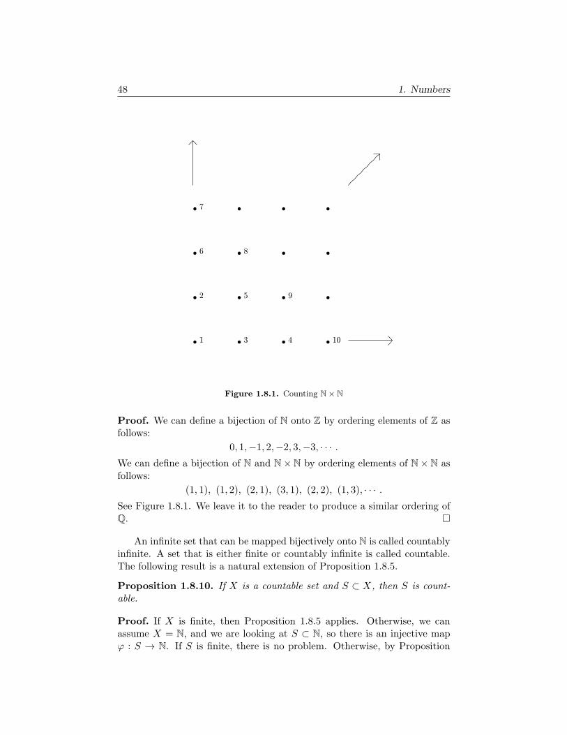
48 1. Numbers
Figure 1.8.1. Counting N× N
Proof. We can define a bijection of N onto Z by ordering elements of Z asfollows:
0, 1,−1, 2,−2, 3,−3, · · · .We can define a bijection of N and N×N by ordering elements of N×N asfollows:
(1, 1), (1, 2), (2, 1), (3, 1), (2, 2), (1, 3), · · · .See Figure 1.8.1. We leave it to the reader to produce a similar ordering ofQ.
An infinite set that can be mapped bijectively onto N is called countablyinfinite. A set that is either finite or countably infinite is called countable.The following result is a natural extension of Proposition 1.8.5.
Proposition 1.8.10. If X is a countable set and S ⊂ X, then S is count-able.
Proof. If X is finite, then Proposition 1.8.5 applies. Otherwise, we canassume X = N, and we are looking at S ⊂ N, so there is an injective mapφ : S → N. If S is finite, there is no problem. Otherwise, by Proposition
1.8. Cardinal numbers 49
1.8.7, there is an injective map ψ : N → S, and then Theorem 1.8.8 impliesthe existence of a bijection between S and N.
There are sets that are not countable; they are said to be uncountable.The following is a key result of G. Cantor.
Proposition 1.8.11. The set R of real numbers is uncountable.
Proof. We may as well show that (0, 1) = x ∈ R : 0 < x < 1 is uncount-able. If it were countable, there would be a bijective map φ : N → (0, 1).Expand the real number φ(j) in its infinite decimal expansion:
(1.8.7) φ(j) =∞∑k=1
ajk · 10−k, ajk ∈ 0, 1, . . . 9.
Now set
(1.8.8)bk = 2 if akk = 2,
3 if akk = 2,
and consider
(1.8.9) ξ =∞∑k=1
bk · 10−k, ξ ∈ (0, 1).
It is seen that ξ is not equal to φ(j) for any j ∈ N, contradicting thehypothesis that φ : N → (0, 1) is onto.
A common notation for the cardinality of R is
(1.8.10) Card(R) = c.
We leave it as an exercise to the reader to show that
(1.8.11) Card(R× R) = c.
Further development of the theory of cardinal numbers requires a for-malization of the notions of set theory. In these notes we have used settheoretical notions rather informally. Our use of such notions has gottensomewhat heavier in this last section. In particular, in the proof of Proposi-tion 1.8.7, the innocent looking use of the phrase “pick x ∈ S . . . ” actuallyassumes a weak version of the Axiom of Choice. For an introduction to theaxiomatic treatment of set theory we refer to [5].
Exercises
1. What is the cardinality of the set P of prime numbers?
50 1. Numbers
2. Let S be a nonempty set and let T be the set of all subsets of S. Adaptthe proof of Proposition 1.8.11 to show that
Card(S) < Card(T ),
i.e., there is not a surjective map φ : S → T .
Hint. There is a natural bijection of T and T , the set of functions f :
S → 0, 1, via f ↔ x ∈ S : f(x) = 1. Given φ : S → T , describe afunction g : S → 0, 1, not in the range of φ, taking a cue from the proofof Proposition 1.8.11.
3. Finish the proof of Proposition 1.8.9.
4. Use the map f(x) = x/(1 + x) to prove that
Card(R+) = Card((0, 1)).
5. Find a one-to-one map of R onto R+ and conclude that Card(R) =Card((0, 1)).
6. Use an interlacing of infinite decimal expansions to prove that
Card((0, 1)× (0, 1)) = Card((0, 1)).
7. Prove (1.8.11).
8. Let m ∈ Z, n ∈ N, and consider
Sm,n = k ∈ Z : m+ 1 ≤ k ≤ m+ n.
Show that
CardSm,n = n.
Hint. Produce a bijective map In → Sm,n.
9. Let S and T be sets. Assume
CardS = m, CardT = n, S ∩ T = ∅,
with m,n ∈ N. Show that
CardS ∪ T = m+ n.
Hint. Produce bijective maps S → Im and T → Sm,n, leading to a bijectionS ∪ T → Im+n.
1.9. Metric properties of R 51
1.9. Metric properties of R
We discuss a number of notions and results related to convergence in R.Recall that a sequence of points (pj) in R converges to a limit p ∈ R (wewrite pj → p) if and only if for every ε > 0 there exists N such that
(1.9.1) j ≥ N =⇒ |pj − p| < ε.
A set S ⊂ R is said to be closed if and only if
(1.9.2) pj ∈ S, pj → p =⇒ p ∈ S.
The complement R \ S of a closed set S is open. Alternatively, Ω ⊂ R isopen if and only if, given q ∈ Ω, there exists ε > 0 such that Bε(q) ⊂ Ω,where
(1.9.3) Bε(q) = p ∈ R : |p− q| < ε,
so q cannot be a limit of a sequence of points in R \ Ω.In particular, the interval
(1.9.4) [a, b] = x ∈ R : a ≤ x ≤ b
is closed, and the interval
(1.9.5) (a, b) = x ∈ R : a < x < b
is open.
We define the closure S of a set S ⊂ R to consist of all points p ∈ Rsuch that Bε(p) ∩ S = ∅ for all ε > 0. Equivalently, p ∈ S if and only ifthere exists an infinite sequence (pj) of points in S such that pj → p. Forexample, the closure of the interval (a, b) is the interval [a, b].
An important property of R is completeness, which we recall is definedas follows. A sequence (pj) of points in R is called a Cauchy sequence if andonly if
(1.9.6) |pj − pk| −→ 0, as j, k → ∞.
It is easy to see that if pj → p for some p ∈ R, then (1.9.6) holds. Thecompleteness property is the converse, given in Theorem 1.6.9, which werecall here.
Theorem 1.9.1. If (pj) is a Cauchy sequence in R, then it has a limit.
Completeness provides a path to the following key notion of compactness.A nonempty set K ⊂ R is said to be compact if and only if the followingproperty holds.
(1.9.7)Each infinite sequence (pj) in K has a subsequence
that converges to a point in K.
52 1. Numbers
It is clear that if K is compact, then it must be closed. It must also bebounded, i.e., there exists R < ∞ such that K ⊂ BR(0). Indeed, if K isnot bounded, there exist pj ∈ K such that |pj+1| ≥ |pj |+ 1. In such a case,|pj −pk| ≥ 1 whenever j = k, so (pj) cannot have a convergent subsequence.The following converse statement is a key result.
Theorem 1.9.2. If a nonempty K ⊂ R is closed and bounded, then it iscompact.
Clearly every nonempty closed subset of a compact set is compact, soTheorem 1.9.2 is a consequence of:
Proposition 1.9.3. Each closed bounded interval I = [a, b] ⊂ R is compact.
Proof. This is a direct consequence of the Bolzano-Weierstrass theorem,Theorem 1.6.10.
Let K ⊂ R be compact. Since K is bounded from above and from below,we have well defined real numbers
(1.9.8) b = supK, a = infK,
the first by Proposition 1.6.12, and the second by a similar argument (cf. Ex-ercise 2 of §1.6). Since a and b are limits of elements of K, we have a, b ∈ K.We use the notation
(1.9.9) b = maxK, a = minK.
We next discuss continuity. If S ⊂ R, a function
(1.9.10) f : S −→ R
is said to be continuous at p ∈ S provided
(1.9.11) pj ∈ S, pj → p =⇒ f(pj) → f(p).
If f is continuous at each p ∈ S, we say f is continuous on S.
The following two results give important connections between continuityand compactness.
Proposition 1.9.4. If K ⊂ R is compact and f : K → R is continuous,then f(K) is compact.
Proof. If (qk) is an infinite sequence of points in f(K), pick pk ∈ K suchthat f(pk) = qk. If K is compact, we have a subsequence pkν → p in K, andthen qkν → f(p) in R.
This leads to the second connection.
1.9. Metric properties of R 53
Proposition 1.9.5. If K ⊂ R is compact and f : K → R is continuous,then there exists p ∈ K such that
(1.9.12) f(p) = maxx∈K
f(x),
and there exists q ∈ K such that
(1.9.13) f(q) = minx∈K
f(x).
Proof. Since f(K) is compact, we have well defined numbers
(1.9.14) b = max f(K), a = min f(K), a, b ∈ f(K).
So take p, q ∈ K such that f(p) = b and f(q) = a.
The next result is called the intermediate value theorem.
Proposition 1.9.6. Take a, b, c ∈ R, a < b. Let f : [a, b] → R be continu-ous. Assume
(1.9.15) f(a) < c < f(b).
Then there exists x ∈ (a, b) such that f(x) = c.
Proof. Let
(1.9.16) S = y ∈ [a, b] : f(y) ≤ c.Then a ∈ S, so S is a nonempty, closed (hence compact) subset of [a, b].Note that b /∈ S. Take
(1.9.17) x = maxS.
Then a < x < b and f(x) ≤ c. If f(x) < c, then there exists ε > 0 such thata < x− ε < x+ ε < b and f(y) < c for x− ε < y < x+ ε. Thus x+ ε ∈ S,contradicting (1.9.17).
Returning to the issue of compactness, we establish some further prop-erties of compact sets K ⊂ R, leading to the important result, Proposition1.9.10 below.
Proposition 1.9.7. Let K ⊂ R be compact. Assume X1 ⊃ X2 ⊃ X3 ⊃ · · ·form a decreasing sequence of closed subsets of K. If each Xm = ∅, then∩mXm = ∅.
Proof. Pick xm ∈ Xm. IfK is compact, (xm) has a convergent subsequence,xmk
→ y. Since xmk: k ≥ ℓ ⊂ Xmℓ
, which is closed, we have y ∈∩mXm.
Corollary 1.9.8. Let K ⊂ R be compact. Assume U1 ⊂ U2 ⊂ U3 ⊂ · · ·form an increasing sequence of open sets in R. If ∪mUm ⊃ K, then UM ⊃ Kfor some M .

54 1. Numbers
Proof. Consider Xm = K \ Um.
Before getting to Proposition 1.9.10, we bring in the following. LetQ denote the set of rational numbers. The set Q ⊂ R has the following“denseness” property: given p ∈ R and ε > 0, there exists q ∈ Q such that|p− q| < ε. Let
(1.9.18) R = Brj (qj) : qj ∈ Q, rj ∈ Q ∩ (0,∞).Note that Q is countable, i.e., it can be put in one-to-one correspondencewith N. Hence R is a countable collection of balls. The following lemma isleft as an exercise for the reader.
Lemma 1.9.9. Let Ω ⊂ R be a nonempty open set. Then
(1.9.19) Ω =∪
B : B ∈ R, B ⊂ Ω.
To state the next result, we say that a collection Uα : α ∈ A covers Kif K ⊂ ∪α∈AUα. If each Uα ⊂ R is open, it is called an open cover of K. IfB ⊂ A and K ⊂ ∪β∈BUβ, we say Uβ : β ∈ B is a subcover. This result iscalled the Heine-Borel theorem.
Proposition 1.9.10. If K ⊂ R is compact, then it has the following prop-erty.
(1.9.20) Every open cover Uα : α ∈ A of K has a finite subcover.
Proof. By Lemma 1.9.9, it suffices to prove the following.
(1.9.21)Every countable cover Bj : j ∈ N of K by open intervals
has a finite subcover.
For this, we set
(1.9.22) Um = B1 ∪ · · · ∪Bm
and apply Corollary 1.9.8.
Exercises
1. Consider a polynomial p(x) = xn + an−1xn−1 + · · · + a1x + a0. Assume
each aj ∈ R and n is odd. Use the intermediate value theorem to show thatp(x) = 0 for some x ∈ R.
We describe the construction of a Cantor set. Take a closed, bounded in-terval [a, b] = C0. Let C1 be obtained from C0 by deleting the open middlethird interval, of length (b − a)/3. At the jth stage, Cj is a disjoint unionof 2j closed intervals, each of length 3−j(b− a). Then Cj+1 is obtained from
1.9. Metric properties of R 55
Cj by deleting the open middle third of each of these 2j intervals. We haveC0 ⊃ C1 ⊃ · · · ⊃ Cj ⊃ · · · , each a closed subset of [a, b].
2. Show that
(1.9.23) C =∩j≥0
Cj
is nonempty, and compact. This is the Cantor set.
3. Suppose C is formed as above, with [a, b] = [0, 1]. Show that points in Care precisely those of the form
(1.9.24) ξ =∞∑j=0
bj 3−j , bj ∈ 0, 2.
4. If p, q ∈ C (and p < q), show that the interval [p, q] must contain pointsnot in C. One says C is totally disconnected.
5. If p ∈ C, ε > 0, show that (p − ε, p + ε) contains infinitely many pointsin C. Given that C is closed, one says C is perfect.
6. Show that Card(C) = Card(R).Hint. With ξ as in (1.9.24) show that
ξ 7→ η =∞∑j=0
(bj2
)2−j
maps C onto [0, 1].
Remark. At this point, we mention theContinuum Hypothesis. If S ⊂ R is uncountable, then CardS = CardR.This hypothesis has been shown not to be amenable to proof or disproof,from the standard axioms of set theory. See [4]. However, there is a largeclass of sets for which the conclusion holds. For example, it holds wheneverS ⊂ R is uncountable and compact. See Exercises 7–9 in §2.3 of Chapter 2for further results along this line.
7. Show that Proposition 1.9.6 implies Proposition 1.7.1.
8. In the setting of Proposition 1.9.6 (the intermediate value theorem),in which f : [a, b] → R is continuous and f(a) < c < f(b), consider thefollowing.
56 1. Numbers
(a) Divide I = [a, b] into two equal intervals Iℓ and Ir, meeting at themidpoint α0 = (a + b)/2. Select I1 = Iℓ if f(α0) ≥ c, I1 = Ir if f(α0) < c.Say I1 = [x1, y1]. Note that f(x1) < c, f(y1) ≥ c.
(b) Divide I1 into two equal intervals I1ℓ and I1r, meeting at the midpoint(x1 + y1)/2 = α1. Select I2 = I1ℓ if f(α1) ≥ c, I2 = I1r if f(α1) < c. SayI2 = [x2, y2]. Note that f(x2) < c, f(y2) ≥ c.
(c) Continue. Having Ik = [xk, yk], of length 2−k(b − a), with f(xk) <c, f(yk) ≥ c, divide Ik into two equal intervals Ikℓ and Ikr, meeting at themidpoint αk = (xk + yk)/2. Select Ik+1 = Ikℓ if f(αk) ≥ c, Ik+1 = Ikr iff(αk) < c. Again, Ik+1 = [xk+1, yk+1] with f(xk+1) < c and f(yk+1) ≥ c.
(d) Show that there exists x ∈ (a, b) such that
xk x, yk x, and f(x) = c.
This method of approximating a solution to f(x) = c is called the bisectionmethod.
1.10. Complex numbers
A complex number is a number of the form
(1.10.1) z = x+ iy, x, y ∈ R,
where the new object i has the property
(1.10.2) i2 = −1.
We denote the set of complex numbers by C. We have R → C, identifyingx ∈ R with x+ i0 ∈ C.
We define addition and multiplication in C as follows. Suppose w =a+ ib, a, b ∈ R. We set
(1.10.3)z + w = (x+ a) + i(y + b),
zw = (xa− yb) + i(xb+ ya).
See Figures 1.10.1 and 1.10.2 for illustrations of these operations.
It is routine to verify various commutative, associative, and distributivelaws, parallel to those in Proposition 1.4.3. If z = 0, i.e., either x = 0 ory = 0, we can set
(1.10.4) z−1 =1
z=
x
x2 + y2− i
y
x2 + y2,
and verify that zz−1 = 1.

1.10. Complex numbers 57
Figure 1.10.1. Addition in the complex plane
For some more notation, for z ∈ C of the form (1.10.1), we set
(1.10.5) z = x− iy, Re z = x, Im z = y.
We say z is the complex conjugate of z, Re z is the real part of z, and Im zis the imaginary part of z.
We next discuss the concept of the magnitude (or absolute value) ofan element z ∈ C. If z has the form (1.10.1), we take a cue from thePythagorean theorem, giving the Euclidean distance from z to 0, and set
(1.10.6) |z| =√x2 + y2.
Note that
(1.10.7) |z|2 = z z.
With this notation, (1.10.4) takes the compact (and clear) form
(1.10.8) z−1 =z
|z|2.
We have
(1.10.9) |zw| = |z| · |w|,
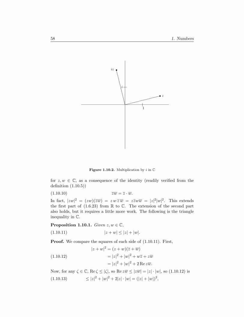
58 1. Numbers
Figure 1.10.2. Multiplication by i in C
for z, w ∈ C, as a consequence of the identity (readily verified from thedefinition (1.10.5))
(1.10.10) zw = z · w.In fact, |zw|2 = (zw)(zw) = z w z w = zzww = |z|2|w|2. This extendsthe first part of (1.6.23) from R to C. The extension of the second partalso holds, but it requires a little more work. The following is the triangleinequality in C.
Proposition 1.10.1. Given z, w ∈ C,
(1.10.11) |z + w| ≤ |z|+ |w|.
Proof. We compare the squares of each side of (1.10.11). First,
(1.10.12)
|z + w|2 = (z + w)(z + w)
= |z|2 + |w|2 + wz + zw
= |z|2 + |w|2 + 2Re zw.
Now, for any ζ ∈ C, Re ζ ≤ |ζ|, so Re zw ≤ |zw| = |z| · |w|, so (1.10.12) is
(1.10.13) ≤ |z|2 + |w|2 + 2|z| · |w| = (|z|+ |w|)2,

1.10. Complex numbers 59
and we have (1.10.11).
We now discuss matters related to convergence in C. Parallel to the realcase, we say a sequence (zj) in C converges to a limit z ∈ C (and writezj → z) if and only if for each ε > 0 there exists N such that
(1.10.14) j ≥ N =⇒ |zj − z| < ε.
Equivalently,
(1.10.15) zj → z ⇐⇒ |zj − z| → 0.
It is easily seen that
(1.10.16) zj → z ⇐⇒ Re zj → Re z and Im zj → Im z.
The set C also has the completeness property, given as follows. A se-quence (zj) in C is said to be a Cauchy sequence if and only if
(1.10.17) |zj − zk| → 0, as j, k → ∞.
It is easy to see (using the triangle inequality) that if zj → z for some z ∈ C,then (1.10.17) holds. Here is the converse:
Proposition 1.10.2. If (zj) is a Cauchy sequence in C, then it has a limit.
Proof. If (zj) is Cauchy in C, then (Re zj) and (Im zj) are Cauchy in R, so,by Theorem 1.6.9, they have limits.
We turn to infinite series∑∞
k=0 ak, with ak ∈ C. We say this convergesif and only if the sequence of partial sums
(1.10.18) Sn =
n∑k=0
ak
converges:
(1.10.19)∞∑k=0
ak = A⇐⇒ Sn → A as n→ ∞.
The following is a useful condition guaranteeing convergence. CompareProposition 1.6.13.
Proposition 1.10.3. The infinite series∑∞
k=0 ak converges provided
(1.10.20)∞∑k=0
|ak| <∞,
i.e., there exists B <∞ such that∑n
k=0 |ak| ≤ B for all n.

60 1. Numbers
Proof. The triangle inequality gives, for ℓ ≥ 1,
(1.10.21)
|Sn+ℓ − Sn| =∣∣∣ n+ℓ∑k=n+1
ak
∣∣∣≤
n+ℓ∑k=n+1
|ak|,
which tends to 0 as n → ∞, uniformly in ℓ ≥ 1, provided (1.10.20) holds(cf. (1.6.42)–(1.6.43)). Hence (1.10.20) ⇒ (Sn) is Cauchy. Convergence thenfollows, by Proposition 1.10.2.
As in the real case, if (1.10.20) holds, we say the infinite series∑∞
k=0 akis absolutely convergent.
An example to which Proposition 1.10.3 applies is the following powerseries, giving the exponential function ez:
(1.10.22) ez =
∞∑k=0
zk
k!, z ∈ C.
Compare Exercise 13 of §1.6. The exponential function is explored in depthin §4.5 of Chapter 4.
We turn to a discussion of polar coordinates on C. Given a nonzeroz ∈ C, we can write
(1.10.23) z = rω, r = |z|, ω =z
|z|.
Then ω has unit distance from 0. If the ray from 0 to ω makes an angle θwith the positive real axis, we have
(1.10.24) Reω = cos θ, Imω = sin θ,
by definition of the trigonometric functions cos and sin. Hence
(1.10.25) z = r cis θ,
where
(1.10.26) cis θ = cos θ + i sin θ.
If also
(1.10.27) w = ρ cisφ, ρ = |w|,
then
(1.10.28) zw = rρ cis(θ + φ),
as a consequence of the identity
(1.10.29) cis(θ + φ) = (cis θ)(cisφ),
1.10. Complex numbers 61
which in turn is equivalent to the pair of trigonometric identities
(1.10.30)cos(θ + φ) = cos θ cosφ− sin θ sinφ,
sin(θ + φ) = cos θ sinφ+ sin θ cosφ.
There is another way to write (1.10.25), using the classical Euler identity
(1.10.31) eiθ = cos θ + i sin θ.
Then (1.10.25) becomes
(1.10.32) z = r eiθ.
The identity (1.10.29) is equivalent to
(1.10.33) ei(θ+φ) = eiθeiφ.
We will present a self-contained derivation of (1.10.31) (and also of (1.10.30)and (1.10.33)) in Chapter 4, §§4.4–4.5. The analysis there includes a precisedescription of what “angle θ” means.
We next define closed and open subsets of C, and discuss the notion ofcompactness. A set S ⊂ C is said to be closed if and only if
(1.10.34) zj ∈ S, zj → z =⇒ z ∈ S.
The complement C \ S of a closed set S is open. Alternatively, Ω ⊂ C isopen if and only if, given q ∈ Ω, there exists ε > 0 such that Bε(q) ⊂ Ω,where
(1.10.35) Bε(q) = z ∈ C : |z − q| < ε,so q cannot be a limit of a sequence of points in C\Ω. We define the closureS of a set S ⊂ C to consist of all points p ∈ C such that Bε(p) ∩ S = ∅ forall ε > 0. Equivalently, p ∈ S if and only if there exists an infinite sequence(pj) of points in S such that pj → p.
Parallel to (1.9.7), we say a nonempty set K ⊂ C is compact if and onlyif the following property holds.
(1.10.36)Each infinite sequence (pj) in K has a subsequence
that converges to a point in K.
As in §1.9, if K ⊂ C is compact, it must be closed and bounded. Parallel toTheorem 1.9.2, we have the converse.
Proposition 1.10.4. If a nonempty K ⊂ C is closed and bounded, then itis compact.
Proof. Let (zj) be a sequence in K. Then (Re zj) and (Im zj) are bounded,so Theorem 1.6.10 implies the existence of a subsequence such that Re zjνand Im zjν converge. Hence the subsequence (zjν ) converges in C. Since Kis closed, the limit must belong to K.
62 1. Numbers
If S ⊂ C, a function
(1.10.37) f : S −→ C
is said to be continuous at p ∈ S provided
(1.10.38) pj ∈ S, pj → p =⇒ f(pj) → f(p).
If f is continuous at each p ∈ S, we say f is continuous on S. The followingresult has the same proof as Proposition 1.9.4.
Proposition 1.10.5. If K ⊂ C is compact and f : K → C is continuous,then f(K) is compact.
Then the following variant of Proposition 1.9.5 is straightforward.
Proposition 1.10.6. If K ⊂ C is compact and f : K → C is continuous,then there exists p ∈ K such that
(1.10.39) |f(p)| = maxz∈K
|f(z)|,
and there exists q ∈ K such that
(1.10.40) |f(q)| = minz∈K
|f(z)|.
There are also straightforward extensions to K ⊂ C of Propositions1.9.7–1.9.10. We omit the details. But see §2.1 of Chapter 2 for furtherextensions.
Exercises
We define π as the smallest positive number such that
cisπ = −1.
See Chapter 4, §§4.4–4.5 for more on this matter.
1. Show that
ω = cis2π
n=⇒ ωn = 1.
For this, use (1.10.29). In conjunction with (1.10.25)–(1.10.28) and Propo-sition 1.7.1, use this to prove the following:
Given a ∈ C, a = 0, n ∈ N, there exist z1, . . . , zn ∈ Csuch that znj = a.
2. Compute (12+
√3
2i)3,
1.10. Complex numbers 63
and verify that
(1.10.41) cosπ
3=
1
2, sin
π
3=
√3
2.
3. Find z1, . . . , zn such that
(1.10.42) znj = 1,
explicitly in the form a+ ib (not simply as cis(2πj/n)), in case
(1.10.43) n = 3, 4, 6, 8.
Hint. Use (1.10.41), and also the fact that the equation u2j = i has solutions
(1.10.44) u1 =1√2+
i√2, u2 = −u1.
4. Take the following path to finding the 5 solutions to
(1.10.45) z5j = 1.
One solution is z1 = 1. Since z5 − 1 = (z− 1)(z4 + z3 + z2 + z+1), we needto find 4 solutions to z4 + z3 + z2 + z + 1 = 0. Write this as
(1.10.46) z2 + z + 1 +1
z+
1
z2= 0,
which, for
(1.10.47) w = z +1
z,
becomes
(1.10.48) w2 + w − 1 = 0.
Use the quadratic formula to find 2 solutions to (1.10.48). Then solve(1.10.47), i.e., z2 − wz + 1 = 0, for z. Use these calculations to show that
cos2π
5=
√5− 1
4.
The roots zj of (1.10.45) form the vertices of a regular pentagon. See Figure1.10.3.
5. Take the following path to explicitly finding the real and imaginary partsof a solution to
z2 = a+ ib.
Namely, with x = Re z, y = Im z, we have
x2 − y2 = a, 2xy = b,

64 1. Numbers
Figure 1.10.3. Regular pentagon, a = (√5− 1)/4.
and also
x2 + y2 = ρ =√a2 + b2,
hence
x =
√ρ+ a
2, y =
b
2x,
as long as a+ ib = −|a|.
6. Taking a cue from Exercise 4 of §1.6, show that
(1.10.49)1
1− z=
∞∑k=0
zk, for z ∈ C, |z| < 1.
7. Show that1
1− z2=
∞∑k=0
z2k, for z ∈ C, |z| < 1.
8. Produce a power series series expansion in z, valid for |z| < 1, for
1
1 + z2.

Chapter 2
Spaces
In Chapter 1 we developed the real number line R, and established a numberof metric properties, such as completeness of R, and compactness of closed,bounded subsets. We also produced the complex plane C, and studied anal-ogous metric properties of C. Here we examine other types of spaces, whichare useful in analysis.
Section 2.1 treats n-dimensional Euclidean space, Rn. This is equippedwith a dot product x · y ∈ R, which gives rise to a norm |x| =
√x · x.
Parallel to (1.6.23) and (1.10.11) of Chapter 1, this norm satisfies the triangleinequality. In this setting, the proof goes through an inequality known asCauchy’s inequality. Then the distance between x and y in Rn is given byd(x, y) = |x−y|, and it satisfies a triangle inequality. With these structures,we have the notion of convergent sequences and Cauchy sequences, and canshow that Rn is complete. There is a notion of compactness for subsets ofRn, similar to that given in (1.9.7) and in (1.10.36) of Chapter 1, for subsetsof R and of C, and it is shown that nonempty, closed bounded subsets of Rn
are compact.
Analysts have found it useful to abstract some of the structures men-tioned above, and apply them to a larger class of spaces, calledmetric spaces.A metric space is a set X, equipped with a distance function d(x, y), satis-fying certain conditions (see (2.2.1)), including the triangle inequality. Forsuch a space, one has natural notions of a convergent sequence and of aCauchy sequence. The space may or may not be complete. If not, thereis a construction of its completion, somewhat similar to the construction ofR as the completion of Q in §1.6 of Chapter 1. We discuss the definitionand some basic properties of metric spaces in §2.2. There is also a naturalnotion of compactness in the metric space context, which we treat in §2.3.
65
66 2. Spaces
Most metric spaces we will encounter are subsets of Euclidean space.One exception introduced in this chapter is the class of infinite products;see (2.3.9). Another important class of metric spaces beyond the Euclideanspace setting consists of spaces of functions, which will be treated in §3.4 ofChapter 3.
2.1. Euclidean spaces
The space Rn, n-dimensional Euclidean space, consists of n-tuples of realnumbers:
(2.1.1) x = (x1, . . . , xn) ∈ Rn, xj ∈ R, 1 ≤ j ≤ n.
The number xj is called the jth component of x. Here we discuss someimportant algebraic and metric structures on Rn. First, there is addition.If x is as in (2.1.1) and also y = (y1, . . . , yn) ∈ Rn, we have
(2.1.2) x+ y = (x1 + y1, . . . , xn + yn) ∈ Rn.
Addition is done componentwise. Also, given a ∈ R, we have
(2.1.3) ax = (ax1, . . . , axn) ∈ Rn.
This is scalar multiplication.
We also have the dot product,
(2.1.4) x · y =n∑
j=1
xjyj = x1y1 + · · ·+ xnyn ∈ R,
given x, y ∈ Rn. The dot product has the properties
(2.1.5)
x · y = y · x,x · (ay + bz) = a(x · y) + b(x · z),x · x > 0 unless x = 0.
Note that
(2.1.6) x · x = x21 + · · ·+ x2n.
We set
(2.1.7) |x| =√x · x,
which we call the norm of x. Note that (2.1.5) implies
(2.1.8) (ax) · (ax) = a2(x · x),
hence
(2.1.9) |ax| = |a| · |x|, for a ∈ R, x ∈ Rn.

2.1. Euclidean spaces 67
Taking a cue from the Pythagorean theorem, we say that the distancefrom x to y in Rn is
(2.1.10) d(x, y) = |x− y|.For us, (2.1.7) and (2.1.10) are simply definitions. We do not need to dependon the Pythagorean theorem. Significant properties will be derived below,without recourse to the Pythagorean theorem.
A set X equipped with a distance function is called a metric space. Wewill consider metric spaces in general in the next section. Here, we want toshow that the Euclidean distance, defined by (2.1.10), satisfies the “triangleinequality,”
(2.1.11) d(x, y) ≤ d(x, z) + d(z, y), ∀x, y, z ∈ Rn.
This in turn is a consequence of the following, also called the triangle in-equality.
Proposition 2.1.1. The norm (2.1.7) on Rn has the property
(2.1.12) |x+ y| ≤ |x|+ |y|, ∀x, y ∈ Rn.
Proof. We compare the squares of the two sides of (2.1.12). First,
(2.1.13)
|x+ y|2 = (x+ y) · (x+ y)
= x · x+ y · x+ y · x+ y · y= |x|2 + 2x · y + |y|2.
Next,
(2.1.14) (|x|+ |y|)2 = |x|2 + 2|x| · |y|+ |y|2.We see that (2.1.12) holds if and only if x · y ≤ |x| · |y|. Thus the proof ofProposition 2.1.1 is finished off by the following result, known as Cauchy’sinequality.
Proposition 2.1.2. For all x, y ∈ Rn,
(2.1.15) |x · y| ≤ |x| · |y|.
Proof. We start with the chain
(2.1.16) 0 ≤ |x− y|2 = (x− y) · (x− y) = |x|2 + |y|2 − 2x · y,which implies
(2.1.17) 2x · y ≤ |x|2 + |y|2, ∀x, y ∈ Rn.
If we replace x by tx and y by t−1y, with t > 0, the left side of (2.1.17) isunchanged, so we have
(2.1.18) 2x · y ≤ t2|x|2 + t−2|y|2, ∀ t > 0.
68 2. Spaces
Now we pick t so that the two terms on the right side of (2.1.18) are equal,namely
(2.1.19) t2 =|y||x|, t−2 =
|x||y|.
(At this point, note that (2.1.15) is obvious if x = 0 or y = 0, so we willassume that x = 0 and y = 0.) Plugging (2.1.19) into (2.1.18) gives
(2.1.20) x · y ≤ |x| · |y|, ∀x, y ∈ Rn.
This is almost (2.1.15). To finish, we can replace x in (2.1.20) by −x =(−1)x, getting
(2.1.21) −(x · y) ≤ |x| · |y|,
and together (2.1.20) and (2.1.21) give (2.1.15).
We now discuss a number of notions and results related to convergencein Rn. First, a sequence of points (pj) in Rn converges to a limit p ∈ Rn (wewrite pj → p) if and only if
(2.1.22) |pj − p| −→ 0,
where | · | is the Euclidean norm on Rn, defined by (2.1.7), and the meaningof (2.1.22) is that for every ε > 0 there exists N such that
(2.1.23) j ≥ N =⇒ |pj − p| < ε.
If we write pj = (p1j , . . . , pnj) and p = (p1, . . . , pn), then (2.1.22) is equiva-lent to
(p1j − p1)2 + · · ·+ (pnj − pn)
2 −→ 0, as j → ∞,
which holds if and only if
|pℓj − pℓ| −→ 0 as j → ∞, for each ℓ ∈ 1, . . . , n.
That is to say, convergence pj → p in Rn is eqivalent to convergence of eachcomponent.
A set S ⊂ Rn is said to be closed if and only if
(2.1.24) pj ∈ S, pj → p =⇒ p ∈ S.
The complement Rn \ S of a closed set S is open. Alternatively, Ω ⊂ Rn isopen if and only if, given q ∈ Ω, there exists ε > 0 such that Bε(q) ⊂ Ω,where
(2.1.25) Bε(q) = p ∈ Rn : |p− q| < ε,
so q cannot be a limit of a sequence of points in Rn \ Ω.
2.1. Euclidean spaces 69
An important property of Rn is completeness, a property defined asfollows. A sequence (pj) of points in Rn is called a Cauchy sequence if andonly if
(2.1.26) |pj − pk| −→ 0, as j, k → ∞.
Again we see that (pj) is Cauchy in Rn if and only if each component isCauchy in R. It is easy to see that if pj → p for some p ∈ Rn, then (2.1.26)holds. The completeness property is the converse.
Theorem 2.1.3. If (pj) is a Cauchy sequence in Rn, then it has a limit,i.e., (2.1.22) holds for some p ∈ Rn.
Proof. Since convergence pj → p in Rn is equivalent to convergence in R ofeach component, the result is a consequence of the completeness of R. Thiswas proved in Chapter 1.
Completeness provides a path to the following key notion of compactness.A nonempty set K ⊂ Rn is said to be compact if and only if the followingproperty holds.
(2.1.27)Each infinite sequence (pj) in K has a subsequence
that converges to a point in K.
It is clear that if K is compact, then it must be closed. It must also bebounded, i.e., there exists R < ∞ such that K ⊂ BR(0). Indeed, if K isnot bounded, there exist pj ∈ K such that |pj+1| ≥ |pj |+ 1. In such a case,|pj −pk| ≥ 1 whenever j = k, so (pj) cannot have a convergent subsequence.The following converse statement is a key result.
Theorem 2.1.4. If a nonempty K ⊂ Rn is closed and bounded, then it iscompact.
Proof. If K ⊂ Rn is closed and bounded, it is a closed subset of some box
(2.1.28) B = (x1, . . . , xn) ∈ Rn : a ≤ xk ≤ b, ∀ k.
Clearly every closed subset of a compact set is compact, so it suffices toshow that B is compact. Now, each closed bounded interval [a, b] in R iscompact, as shown in §1.9 of Chapter 1, and (by reasoning similar to theproof of Theorem 2.1.3) the compactness of B follows readily from this.
We establish some further properties of compact sets K ⊂ Rn, leadingto the important result, Proposition 2.1.8 below. This generalizes resultsestablished for n = 1 in §1.9 of Chapter 1. A further generalization will begiven in §2.3.
70 2. Spaces
Proposition 2.1.5. Let K ⊂ Rn be compact. Assume X1 ⊃ X2 ⊃ X3 ⊃ · · ·form a decreasing sequence of closed subsets of K. If each Xm = ∅, then∩mXm = ∅.
Proof. Pick xm ∈ Xm. IfK is compact, (xm) has a convergent subsequence,xmk
→ y. Since xmk: k ≥ ℓ ⊂ Xmℓ
, which is closed, we have y ∈∩mXm.
Corollary 2.1.6. Let K ⊂ Rn be compact. Assume U1 ⊂ U2 ⊂ U3 ⊂ · · ·form an increasing sequence of open sets in Rn. If ∪mUm ⊃ K, then UM ⊃K for some M .
Proof. Consider Xm = K \ Um.
Before getting to Proposition 2.1.8, we bring in the following. Let Qdenote the set of rational numbers, and let Qn denote the set of points inRn all of whose components are rational. The set Qn ⊂ Rn has the following“denseness” property: given p ∈ Rn and ε > 0, there exists q ∈ Qn suchthat |p− q| < ε. Let
(2.1.29) R = Br(q) : q ∈ Qn, r ∈ Q ∩ (0,∞).Note that Q and Qn are countable, i.e., they can be put in one-to-one corre-spondence with N. Hence R is a countable collection of balls. The followinglemma is left as an exercise for the reader.
Lemma 2.1.7. Let Ω ⊂ Rn be a nonempty open set. Then
(2.1.30) Ω =∪
B : B ∈ R, B ⊂ Ω.
To state the next result, we say that a collection Uα : α ∈ A covers Kif K ⊂ ∪α∈AUα. If each Uα ⊂ Rn is open, it is called an open cover of K. IfB ⊂ A and K ⊂ ∪β∈BUβ, we say Uβ : β ∈ B is a subcover.
Proposition 2.1.8. If K ⊂ Rn is compact, then it has the following prop-erty.
(2.1.31) Every open cover Uα : α ∈ A of K has a finite subcover.
Proof. By Lemma 2.1.7, it suffices to prove the following.
(2.1.32)Every countable cover Bj : j ∈ N of K by open balls
has a finite subcover.
To see this, write R = Bj : j ∈ N. Given the cover Uα, pass toBj : j ∈ J, where j ∈ J if and only of Bj is contained in some Uα.By (2.1.30), Bj : j ∈ J covers K. If (2.1.32) holds, we have a subcoverBℓ : ℓ ∈ L for some finite L ⊂ J . Pick αℓ ∈ A such that Bℓ ⊂ Uαℓ
. TheUαℓ
: ℓ ∈ L is the desired finite subcover advertised in (2.1.31).
2.1. Euclidean spaces 71
Finally, to prove (2.1.32), we set
(2.1.33) Um = B1 ∪ · · · ∪Bm
and apply Corollary 2.1.6.
Exercises
1. Identifying z = x + iy ∈ C with (x, y) ∈ R2 and w = u + iv ∈ C with(u, v) ∈ R2, show that the dot product satisfies
z · w = Re zw.
In light of this, compare the proof of Proposition 2.1.1 with that of Propo-sition 1.10.1 in Chapter 1.
2. Show that the inequality (2.1.12) implies (2.1.11).
3. Given x, y ∈ Rn, we say x is orthogonal to y (x ⊥ y) provided x · y = 0.Show that, for x, y ∈ Rn,
x ⊥ y ⇐⇒ |x+ y|2 = |x|2 + |y|2.
4. Let e1, v ∈ Rn and assume |e1| = |v| = 1. Show that
e1 − v ⊥ e1 + v.
Hint. Expand (e1 − v) · (e1 + v).See Figure 2.1.1 for the geometrical significance of this, when n = 2.
5. Let S1 = x ∈ R2 : |x| = 1 denote the unit circle in R2, and sete1 = (1, 0) ∈ S1. Pick a ∈ R such that 0 < a < 1, and set u = (1 − a)e1.See Figure 2.1.2. Then pick
v ∈ S1 such that v − u ⊥ e1, and set b = |v − e1|.
Show that
(2.1.34) b =√2a.
Hint. Note that 1− a = u · e1 = v · e1, hence a = 1− v · e1.Then expand b2 = (v − e1) · (v − e1).

72 2. Spaces
Figure 2.1.1. Right triangle in a circle
6. Recall the approach to (2.1.34) in classical Euclidean geometry, usingsimilarity of triangles, leading to
a
b=b
2.
What is the relevance of Exercise 4 to this?
In Classical Euclidean geometry, the point v is constructed as the in-tersection of a line (through u, perpendicular to the line from 0 to e1) andthe circle S1. What is the advantage of the material developed here (involv-ing completeness of R) over the axioms of Euclid in guaranteeing that thisintersection exists?
7. Prove Lemma 2.1.7.
8. Use Proposition 2.1.8 to prove the following extension of Proposition2.1.5.
Proposition 2.1.9. Let K ⊂ Rn be compact. Assume Xα : α ∈ A is acollection of closed subsets of K. Assume that for each finite set B ⊂ A,
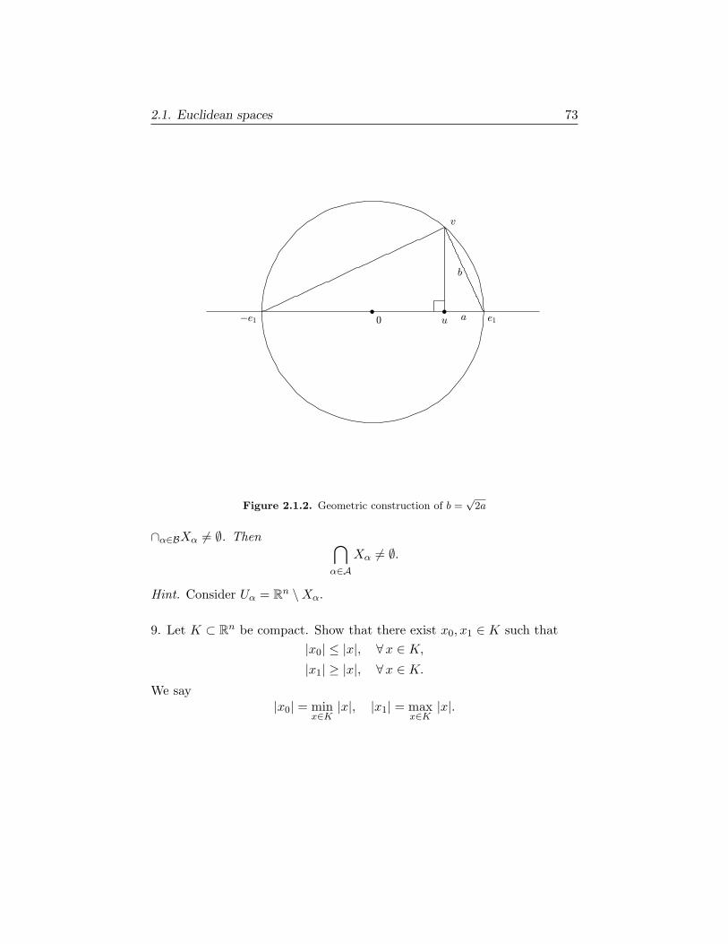
2.1. Euclidean spaces 73
Figure 2.1.2. Geometric construction of b =√2a
∩α∈BXα = ∅. Then ∩α∈A
Xα = ∅.
Hint. Consider Uα = Rn \Xα.
9. Let K ⊂ Rn be compact. Show that there exist x0, x1 ∈ K such that
|x0| ≤ |x|, ∀x ∈ K,
|x1| ≥ |x|, ∀x ∈ K.
We say|x0| = min
x∈K|x|, |x1| = max
x∈K|x|.
74 2. Spaces
2.2. Metric spaces
A metric space is a set X, together with a distance function d : X ×X →[0,∞), having the properties that
(2.2.1)
d(x, y) = 0 ⇐⇒ x = y,
d(x, y) = d(y, x),
d(x, y) ≤ d(x, z) + d(y, z).
The third of these properties is called the triangle inequality. We sometimesdenote this metric space by (X, d). An example of a metric space is the setof rational numbers Q, with d(x, y) = |x− y|. Another example is X = Rn,with
d(x, y) =√(x1 − y1)2 + · · ·+ (xn − yn)2.
This was treated in §2.1.If (xν) is a sequence in X, indexed by ν = 1, 2, 3, . . . , i.e., by ν ∈ Z+,
one says
(2.2.2) xν → y ⇐⇒ d(xν , y) → 0, as ν → ∞.
One says (xν) is a Cauchy sequence if and only if
(2.2.3) d(xν , xµ) → 0 as µ, ν → ∞.
One says X is a complete metric space if every Cauchy sequence convergesto a limit in X. Some metric spaces are not complete; for example, Q isnot complete. You can take a sequence (xν) of rational numbers such thatxν →
√2, which is not rational. Then (xν) is Cauchy in Q, but it has no
limit in Q.If a metric space X is not complete, one can construct its completion X
as follows. Let an element ξ of X consist of an equivalence class of Cauchysequences in X, where we say
(2.2.4) (xν) ∼ (x′ν) =⇒ d(xν , x′ν) → 0.
We write the equivalence class containing (xν) as [xν ]. If ξ = [xν ] and η =[yν ], we can set
(2.2.5) d(ξ, η) = limν→∞
d(xν , yν),
and verify that this is well defined, and makes X a complete metric space.Details are provided at the end of this section.
If the completion of Q is constructed by this process, you get R, the setof real numbers. This construction was carried out in §1.6 of Chapter 1.
There are a number of useful concepts related to the notion of closeness.We define some of them here. First, if p is a point in a metric space X and
2.2. Metric spaces 75
r ∈ (0,∞), the set
(2.2.6) Br(p) = x ∈ X : d(x, p) < r
is called the open ball about p of radius r. Generally, a neighborhood ofp ∈ X is a set containing such a ball, for some r > 0.
A set S ⊂ X is said to be closed if and only if
(2.2.7) pj ∈ S, pj → p =⇒ p ∈ S.
The complement X \ S of a closed set is said to be open. Alternatively,U ⊂ X is open if and only if
(2.2.8) q ∈ U =⇒ ∃ ε > 0 such that Bε(q) ⊂ U,
so q cannot be a limit of a sequence of points in X \ U .
We state a couple of straightforward propositions, whose proofs are leftto the reader.
Proposition 2.2.1. If Uα is a family of open sets in X, then ∪αUα is open.If Kα is a family of closed subsets of X, then ∩αKα is closed.
Given S ⊂ X, we denote by S (the closure of S) the smallest closedsubset of X containing S, i.e., the intersection of all the closed sets Kα ⊂ Xcontaining S. The following result is straightforward.
Proposition 2.2.2. Given S ⊂ X, p ∈ S if and only if there exist xj ∈ Ssuch that xj → p.
Given S ⊂ X, p ∈ X, we say p is an accumulation point of S if and onlyif, for each ε > 0, there exists q ∈ S ∩ Bε(p), q = p. It follows that p is anaccumulation point of S if and only if each Bε(p), ε > 0, contains infinitelymany points of S. One straightforward observation is that all points of S \Sare accumulation points of S.
If S ⊂ Y ⊂ X, we say S is dense in Y provided S ⊃ Y .
The interior of a set S ⊂ X is the largest open set contained in S, i.e.,the union of all the open sets contained in S. Note that the complement ofthe interior of S is equal to the closure of X \ S.
We next define the notion of a connected space. A metric space X issaid to be connected provided that it cannot be written as the union of twodisjoint nonempty open subsets. The following is a basic example. Here, wetreat I as a stand-alone metric space.
Proposition 2.2.3. Each interval I in R is connected.
Proof. Suppose A ⊂ I is nonempty, with nonempty complementB ⊂ I, andboth sets are open. (Hence both sets are closed.) Take a ∈ A, b ∈ B; we can
76 2. Spaces
assume a < b. (Otherwise, switch A and B.) Let ξ = supx ∈ [a, b] : x ∈ A.This exists, by Proposition 1.6.12 of Chapter 1.
Now we obtain a contradiction, as follows. Since A is closed, ξ ∈ A.(Hence ξ < b.) But then, since A is open, ξ > a, and furthermore theremust be a neighborhood (ξ − ε, ξ + ε) contained in A. This would implyξ ≥ ξ + ε. Contradiction.
See the next chapter for more on connectedness, and its connection tothe Intermediate Value Theorem.
Construction of the completion of (X, d)
As indicated earlier in this section, if (X, d) is a metric space, we can
construct its completion (X, d). This construction can be compared to that
done to pass from Q to R in §1.6 of Chapter 1. Elements of X consistof equivalence classes of Cauchy sequences in X, with equivalence relationgiven by (2.2.4). To verify that (2.2.4) defines an equivalence relation, weneed to show that the relation specified there is reflexive, symmetric, andtransitive. The first two properties are completely straightforward. As forthe third, we need to show that
(2.2.9) (xν) ∼ (x′ν), (x′ν) ∼ (x′′ν) =⇒ (xν) ∼ (x′′ν).
In fact, the triangle inequality for d gives
(2.2.10) d(xν , x′′ν) ≤ d(xν , x
′ν) + d(x′ν , x
′′ν),
from which (2.2.9) readily follows. We write the equivalence class containing(xν) as [xν ].
Given ξ = [xν ] and η = [yν ], we propose to define d(ξ, η) by
(2.2.11) d(ξ, η) = limν→∞
d(xν , yν).
To obtain a well defined d : X×X → [0,∞), we need to verify that the limiton the right side of (2.2.11) exists whenever (xν) and (yν) are Cauchy in X,and that the limit is unchanged if (xν) and (yν) are replaced by (x′ν) ∼ (xν)and (y′ν) ∼ (yν). First, we show that dν = d(xν , yν) is a Cauchy sequence inR. The triangle inequality for d gives
dν = d(xν , yν) ≤ d(xν , xµ) + d(xµ, yµ) + d(yµ, yν),
hence
dν − dµ ≤ d(xν , xµ) + d(yµ, yν),
2.2. Metric spaces 77
and the same upper estimate applies to dµ − dν , hence to |dν − dµ|. Thusthe limit on the right side of (2.2.11) exists. Next, with d′ν = d(x′ν , y
′ν), we
have
d′ν = d(x′ν , y′ν) ≤ d(x′ν , xν) + d(xν , yν) + d(yν , y
′ν),
hence
d′ν − dν ≤ d(x′ν , xν) + d(yν , y′ν),
and the same upper estimate applies to dν − d′ν , hence to |d′ν − dν |.These observations establish that d : X × X → [0,∞) is well defined.
We next need to show that it makes X a metric space. First,
(2.2.12) d(ξ, η) = 0 ⇒ limν→∞
d(xν , yν) = 0 ⇒ (xν) ∼ (yν) ⇒ ξ = η.
Next, the symmetry d(ξ, η) = d(η, ξ) follows from (2.2.11) and the symmetry
of d. Finally, if also ζ = [zν ] ∈ X, then
(2.2.13)
d(ξ, ζ) = limνd(xν , zν)
≤ limν
[d(xν , yν) + d(yν , zν)
]= d(ξ, η) + d(η, ζ),
so d satisfies the triangle inequality.
To proceed, we have a natural map
(2.2.14) j : X −→ X, j(x) = (x, x, x, . . . ).
It is clear that for each x, y ∈ X,
(2.2.15) d(j(x), j(y)) = d(x, y).
From here on, we will simply identify a point x ∈ X with its image j(x) ∈ X,
using the notation x ∈ X (so X ⊂ X). It is useful to observe that if (xk) isa Cauchy sequence in X, then
(2.2.16) ξ = [xk] =⇒ limk→∞
d(ξ, xk) = 0.
In fact,
(2.2.17) d(ξ, xk) = limν→∞
d(xν , xk) → 0 as k → ∞.
From here we have the following.
Lemma 2.2.4. The set X is dense in X.
Proof. Given ξ ∈ X, say ξ = [xν ], the fact that xν → ξ in (X, d) followsfrom (2.2.16).
We are now ready for the following analogue of Theorem 1.6.9 of Chapter1.
78 2. Spaces
Proposition 2.2.5. The metric space (X, d) is complete.
Proof. Assume (ξk) is Cauchy in (X, d). By Lemma 2.2.4, we can pick
xk ∈ X such that d(ξk, xk) ≤ 2−k. We claim (xk) is Cauchy in X. In fact,
(2.2.18)
d(xk, xℓ) = d(xk, xℓ)
≤ d(xk, ξk) + d(ξk, ξℓ) + d(ξℓ, xℓ)
≤ d(ξk, ξℓ) + 2−k + 2−ℓ,
so
(2.2.19) d(xk, xℓ) −→ 0 as k, ℓ→ ∞.
Since (xk) is Cauchy in X, it defines an element ξ = [xk] ∈ X. We claimξk → ξ. In fact,
(2.2.20)d(ξk, ξ) ≤ d(ξk, xk) + d(xk, ξ)
≤ d(xk, ξ) + 2−k,
and the fact that d(xk, ξ) → 0 as k → ∞ follows from (2.2.17). Thiscompletes the proof of Proposition 2.2.5.
Exercises
1. Prove Proposition 2.2.1.
2. Prove Proposition 2.2.2.
3. Suppose the metric space (X, d) is complete, and (X, d) is constructedas indicated in (2.2.4)–(2.2.5), and described in detail in (2.2.9)–(2.2.17).
Show that the natural inclusion j : X → X is both one-to-one and onto.
4. Show that if p ∈ Rn and R > 0, the ball BR(p) = x ∈ Rn : |x− p| < Ris connected.Hint. Suppose BR(p) = U ∪ V , a union of two disjoint open sets. Givenq1 ∈ U, q2 ∈ V , consider the line segment
ℓ = tq1 + (1− t)q2 : 0 ≤ t ≤ 1.
5. Let X = Rn, but replace the distance
d(x, y) =√
(x1 − y1)2 + · · ·+ (xn − yn)2

2.2. Metric spaces 79
by
d1(x, y) = |x1 − y1|+ · · ·+ |xn − yn|.Show that (X, d1) is a metric space. In particular, verify the triangle in-equality. Show that a sequence pj converges in (X, d1) if and only if itconverges in (X, d).
6. Show that if U is an open subset of (X, d), then U is a union of openballs.
7. Let S ⊂ X be a dense subset. Let
B = Br(p) : p ∈ S, r ∈ Q+,
with Br(p) defined as in (2.2.6). Show that if U is an open subset of X,then U is a union of balls in B. That is, if q ∈ U , there exists B ∈ B suchthat q ∈ B ⊂ U .
Given a nonempty metric space (X, d), we say it is perfect if it is completeand has no isolated points. Exercises 8–10 deal with perfect metric spaces.
8. Show that if p ∈ X and ε > 0, then Bε(p) contains infinitely many points.
9. Pick distinct p0, p1 ∈ X, and take positive r0 < (1/2)d(p0, p1). Show that
X0 = Br0(p0) and X1 = Br0(p1)
are disjoint perfect subsets of X (i.e., are each perfect metric spaces).
10. Similarly, take distinct p00, p01 ∈ X0 and distinct p10, p11 ∈ X1, andsufficiently small r1 > 0 such that
Xjk = Br1(pjk) for k = 0, 1 are disjoint perfect subsets of Xj .
Continue in this fashion, producing Xj1···jk+1⊂ Xj1···jk , closed balls of radius
rk 0, centered at pj1···jk+1. Show that you can define a function
φ :∞∏ℓ=1
0, 1 → X, φ((j1, j2, j3, . . . )) = limk→∞
pj1j2···jk .
Show that φ is one-to-one, and deduce that
Card(X) ≥ Card(R).
A metric space X is said to be separable if it has a countable dense subset.
80 2. Spaces
11. Let X be a separable metric space, with a dense subset S = pj : j ∈ N.Produce a function
ψ : X −→∞∏ℓ=1
N
as follows. Given x ∈ X, choose a sequence (pjν ) of points in S such thatpjν → x. Set
ψ(x) = (j1, j2, j3, . . . ).
Show that ψ is one-to-one, and deduce that
Card(X) ≤ Card(R).
2.3. Compactness
We return to the notion of compactness, defined in the Euclidean contextin (2.1.27). We say a (nonempty) metric space X is compact provided thefollowing property holds:
(2.3.1) Each sequence (xk) in X has a convergent subsequence.
We will establish various properties of compact metric spaces, and providevarious equivalent characterizations. For example, it is easily seen that(2.3.1) is equivalent to:
(2.3.2) Each infinite subset S ⊂ X has an accumulation point.
The following property is known as total boundedness:
Proposition 2.3.1. If X is a compact metric space, then
(2.3.3)Given ε > 0, ∃ finite set x1, . . . , xN such that
Bε(x1), . . . , Bε(xN ) covers X.
Proof. Take ε > 0 and pick x1 ∈ X. If Bε(x1) = X, we are done. If not,pick x2 ∈ X \ Bε(x1). If Bε(x1) ∪ Bε(x2) = X, we are done. If not, pickx3 ∈ X\[Bε(x1)∪Bε(x2)]. Continue, taking xk+1 ∈ X\[Bε(x1)∪· · ·∪Bε(xk)],if Bε(x1) ∪ · · · ∪Bε(xk) = X. Note that, for 1 ≤ i, j ≤ k,
i = j =⇒ d(xi, xj) ≥ ε.
If one never covers X this way, consider S = xj : j ∈ N. This is an infiniteset with no accumulation point, so property (2.3.2) is contradicted.
Corollary 2.3.2. If X is a compact metric space, it has a countable densesubset.
Proof. Given ε = 2−n, let Sn be a finite set of points xj such that Bε(xj)covers X. Then C = ∪nSn is a countable dense subset of X.
2.3. Compactness 81
Here is another useful property of compact metric spaces, which willeventually be generalized even further, in (2.3.6) below.
Proposition 2.3.3. Let X be a compact metric space. Assume K1 ⊃ K2 ⊃K3 ⊃ · · · form a decreasing sequence of closed subsets of X. If each Kn = ∅,then ∩nKn = ∅.
Proof. Pick xn ∈ Kn. If (2.3.1) holds, (xn) has a convergent subsequence,xnk
→ y. Since xnk: k ≥ ℓ ⊂ Knℓ
, which is closed, we have y ∈ ∩nKn.
Corollary 2.3.4. Let X be a compact metric space. Assume U1 ⊂ U2 ⊂U3 ⊂ · · · form an increasing sequence of open subsets of X. If ∪nUn = X,then UN = X for some N .
Proof. Consider Kn = X \ Un.
The following is an important extension of Corollary 2.3.4. Note howthis generalizes Proposition 2.1.8.
Proposition 2.3.5. If X is a compact metric space, then it has the property:
(2.3.4) Every open cover Uα : α ∈ A of X has a finite subcover.
Proof. Let C = zj : j ∈ N ⊂ X be a countable dense subset of X, asin Corollary 2.3.2. Given p ∈ Uα, there exist zj ∈ C and a rational rj > 0such that p ∈ Brj (zj) ⊂ Uα. Hence each Uα is a union of balls Brj (zj), withzj ∈ C ∩ Uα, rj rational. Thus it suffices to show that
(2.3.5)Every countable cover Bj : j ∈ N of X
by open balls has a finite subcover.
Compare the argument used in Proposition 2.1.8. To prove (2.3.5), we set
Un = B1 ∪ · · · ∪Bn
and apply Corollary 2.3.4.
The following is a convenient alternative to property (2.3.4):
(2.3.6)If Kα ⊂ X are closed and
∩α
Kα = ∅,
then some finite intersection is empty.
Considering Uα = X \Kα, we see that
(2.3.4) ⇐⇒ (2.3.6).
The following result, known as the Heine-Borel theorem, completes Propo-sition 2.3.5.
82 2. Spaces
Theorem 2.3.6. For a metric space X,
(2.3.1) ⇐⇒ (2.3.4).
Proof. By Proposition 2.3.5, (2.3.1) ⇒ (2.3.4). To prove the converse, itwill suffice to show that (2.3.6) ⇒ (2.3.2). So let S ⊂ X and assume S hasno accumulation point. We claim:
Such S must be closed.
Indeed, if z ∈ S and z /∈ S, then z would have to be an accumulation point.To proceed, say S = xα : α ∈ A, and set Kα = S \ xα. Then each Kα
has no accumulation point, hence Kα ⊂ X is closed. Also ∩αKα = ∅. Hencethere exists a finite set F ⊂ A such that ∩α∈FKα = ∅, if (2.3.6) holds.Hence S = ∪α∈Fxα is finite, so indeed (2.3.6) ⇒ (2.3.2).
Remark. So far we have that for every metric space X,
(2.3.1) ⇐⇒ (2.3.2) ⇐⇒ (2.3.4) ⇐⇒ (2.3.6) =⇒ (2.3.3).
We claim that (2.3.3) implies the other conditions if X is complete. Ofcourse, compactness implies completeness, but (2.3.3) may hold for incom-plete X, e.g., X = (0, 1) ⊂ R.
Proposition 2.3.7. If X is a complete metric space with property (2.3.3),then X is compact.
Proof. It suffices to show that (2.3.3) ⇒ (2.3.2) if X is a complete metricspace. So let S ⊂ X be an infinite set. Cover X by balls
B1/2(x1), . . . , B1/2(xN ).
One of these balls contains infinitely many points of S, and so does itsclosure, say X1 = B1/2(y1). Now cover X by finitely many balls of radius1/4; their intersection with X1 provides a cover of X1. One such set contains
infinitely many points of S, and so does its closure X2 = B1/4(y2) ∩ X1.Continue in this fashion, obtaining
X1 ⊃ X2 ⊃ X3 ⊃ · · · ⊃ Xk ⊃ Xk+1 ⊃ · · · , Xj ⊂ B2−j (yj),
each containing infinitely many points of S. Pick zj ∈ Xj . One sees that(zj) forms a Cauchy sequence. If X is complete, it has a limit, zj → z, andz is seen to be an accumulation point of S.
Remark. Note the similarity of this argument with the proof of the Bolzano-Weiersrass theorem in Chapter 1.
2.3. Compactness 83
If Xj , 1 ≤ j ≤ m, is a finite collection of metric spaces, with metrics dj ,we can define a Cartesian product metric space
(2.3.7) X =
m∏j=1
Xj , d(x, y) = d1(x1, y1) + · · ·+ dm(xm, ym).
Another choice of metric is δ(x, y) =√d1(x1, y1)2 + · · ·+ dm(xm, ym)2. The
metrics d and δ are equivalent, i.e., there exist constants C0, C1 ∈ (0,∞)such that
(2.3.8) C0δ(x, y) ≤ d(x, y) ≤ C1δ(x, y), ∀ x, y ∈ X.
A key example is Rm, the Cartesian product of m copies of the real line R.We describe some important classes of compact spaces.
Proposition 2.3.8. If Xj are compact metric spaces, 1 ≤ j ≤ m, so isX =
∏mj=1Xj .
Proof. If (xν) is an infinite sequence of points inX, say xν = (x1ν , . . . , xmν),pick a convergent subsequence of (x1ν) inX1, and consider the correspondingsubsequence of (xν), which we relabel (xν). Using this, pick a convergentsubsequence of (x2ν) in X2. Continue. Having a subsequence such thatxjν → yj inXj for each j = 1, . . . ,m, we then have a convergent subsequencein X.
The following result is useful for analysis on Rn.
Proposition 2.3.9. If K is a closed bounded subset of Rn, then K is com-pact.
Proof. This has been proved in §2.1. There it was noted that the resultfollows from the compactness of a closed bounded interval I = [a, b] in R,which in turn was proved in §1.9 of Chapter 1. Here, we just note thatcompactness of [a, b] is also a corollary of Proposition 2.3.7.
We next give a slightly more sophisticated result on compactness. Thefollowing extension of Proposition 2.3.8 is a special case of Tychonov’s The-orem.
Proposition 2.3.10. If Xj : j ∈ Z+ are compact metric spaces, so isX =
∏∞j=1Xj .
Here, we can make X a metric space by setting
(2.3.9) d(x, y) =
∞∑j=1
2−j dj(pj(x), pj(y))
1 + dj(pj(x), pj(y)),

84 2. Spaces
where pj : X → Xj is the projection onto the jth factor. It is easy to verifythat, if xν ∈ X, then xν → y in X, as ν → ∞, if and only if, for eachj, pj(xν) → pj(y) in Xj .
Proof. Following the argument in Proposition 2.3.8, if (xν) is an infinitesequence of points in X, we obtain a nested family of subsequences
(2.3.10) (xν) ⊃ (x1ν) ⊃ (x2ν) ⊃ · · · ⊃ (xjν) ⊃ · · ·
such that pℓ(xjν) converges in Xℓ, for 1 ≤ ℓ ≤ j. The next step is a diagonal
construction. We set
(2.3.11) ξν = xνν ∈ X.
Then, for each j, after throwing away a finite number N(j) of elements, oneobtains from (ξν) a subsequence of the sequence (xjν) in (2.3.10), so pℓ(ξν)converges in Xℓ for all ℓ. Hence (ξν) is a convergent subsequence of (xν).
Exercises
1. Let φ : [0,∞) → [0,∞) have the following properties: Assume
φ(0) = 0, φ(s) < φ(s+ t) ≤ φ(s) + φ(t), for s ≥ 0, t > 0.
Prove that if d(x, y) is symmetric and satisfies the triangle inequality, sodoes
δ(x, y) = φ(d(x, y)).
2. Show that the function d(x, y) defined by (2.3.9) satisfies (2.2.1).Hint. Consider φ(r) = r/(1 + r).
3. In the setting of (2.3.7), let
δ(x, y) =d1(x1, y1)
2 + · · ·+ dm(xm, ym)21/2
.
Show that
δ(x, y) ≤ d(x, y) ≤√mδ(x, y).
4. Let X be a metric space, p ∈ X, and let K ⊂ X be compact. Show thatthere exist x0, x1 ∈ K such that
d(x0, p) ≤ d(x, p), ∀x ∈ K,
d(x1, p) ≥ d(x, p), ∀x ∈ K.
2.4. The Baire category theorem 85
Show that there exist y0, y1 ∈ K such that
d(q0, q1) ≤ d(y0, y1), ∀ q0, q1 ∈ K.
We say diamK = d(y0, y1).
5. Let X be a metric space that satisfies the total boundedness condition
(2.3.3), and let X be its completion. Show that X is compact.
Hint. Show that X also satisfies condition (2.3.3).
6. Deduce from Exercises 10 and 11 of §2.2 that if X is a compact metricspace with no isolated points, then Card(X) = Card(R). Note how thisgeneralizes the result on Cantor sets in Exercise 6, §1.9, of Chapter 1.
In Exercises 7–9, X is an uncountable compact metric space (so, by Exercise11 of §2.2, CardX ≤ CardR).
7. Define K ⊂ X as follows:
x ∈ K ⇐⇒ Bε(x) is uncountable, ∀ ε > 0.
Show that(a) K = ∅.Hint. Cover X with B1(pj), 1 ≤ j ≤ N0. At least one is uncountable; call
it X0. Cover X0 with X0 ∩ B1/2(pj), 1 ≤ j ≤ N1, pj ∈ X0. At least oneis uncountable; call it X1. Continue, obtaining uncountable compact setsX0 ⊃ X1 ⊃ · · · , with diamXj ≤ 21−j . Show that ∩jXj = x with x ∈ K.
8. In the setting of Exercise 7, show that(b) K is closed (hence compact), and(c) K has no isolated points.Hint for (c). Given x ∈ K, show that, for each ε > 0, there exists δ ∈ (0, ε)
such that Bε(x) \ Bδ(X) is uncountable. Apply Exercise 7 to this compactmetric space.
9. Deduce from Exercises 6–8 that CardK = CardR. Hence conclude that
CardX = CardR.
2.4. The Baire category theorem
If X is a metric space, a subset U ⊂ X is said to be dense if U = X, and asubset S ⊂ X is said to be nowhere dense if S contains no nonempty openset. Consequently, S is nowhere dense if and only if X \ S is dense. Also,
86 2. Spaces
a set U ⊂ X is dense in X if and only if U intersects each nonempty opensubset of X.
Our main goal here is to prove the following.
Theorem 2.4.1. A complete metric space X cannot be written as a count-able union of nowhere dense subsets.
Proof. Let Sk ⊂ X be nowhere dense, k ∈ N. Set
(2.4.1) Tk =k∪
j=1
Sj ,
so Tk are closed, nowhere dense, and increasing. Consider
(2.4.2) Uk = X \ Tk,which are open, dense, and decreasing. Clearly
(2.4.3)∪k
Sk = X =⇒∩k
Uk = ∅,
so to prove the theorem, we show that there exists p ∈ ∩kUk.
To do this, pick p1 ∈ U1 and ε1 > 0 such that Bε1(p1) ⊂ U1. Since U2 isdense in X, we can then pick p2 ∈ Bε1(p1)∩U2 and ε2 ∈ (0, ε1/2) such that
(2.4.4) Bε2(p2) ⊂ Bε1(p1) ∩ U2.
Continue, producing pk ∈ Bεk−1(pk−1) ∩ Uk and εk 0 such that
(2.4.5) Bεk(pk) ⊂ Bεk−1(pk−1) ∩ Uk,
which is possible at each stage because Uk is dense inX, and hence intersectseach nonempty open set. Note that
(2.4.6) pℓ ∈ Bεℓ(pℓ) ⊂ Bεk(pk), ∀ ℓ > k.
It follows that
(2.4.7) d(pℓ, pk) ≤ εk, ∀ ℓ > k,
so (pk) is Cauchy. Since X is complete, this sequence has a limit p ∈ X.
Since each Bεk(pk) is closed, (2.4.6) implies
(2.4.8) p ∈ Bεk(pk) ⊂ Uk, ∀ k.This finishes the proof.
Theorem 2.4.1 is called the Baire category theorem. The terminologyarises as follows. We say a subset Y ⊂ X is of first category provided Y isa countable union of nowhere dense sets. If Y is not a set of first category,we say it is of second category. Theorem 2.4.1 says that if X is a completemetric space, then X is of second category.
Chapter 3
Functions
The playing fields for analysis are spaces, and the players themselves arefunctions. In this chapter we develop some frameworks for understandingthe behavior of various classes of functions. We spend about half the chapterstudying functions f : X → Y from one metric space (X) to another (Y ),and about half specializing to the case Y = Rn.
Our emphasis is on continuous functions, and §3.1 presents a number ofresults on continuous functions f : X → Y , which by definition have theproperty
xν → x =⇒ f(xν) → f(x).
We devote particular attention to the behavior of continuous functions oncompact sets. We bring in the notion of uniform continuity, a priori strongerthan continuity, and show that f continuous onX ⇒ f uniformly continuouson X, provided X is compact. We also introduce the notion of connected-ness, and extend the intermediate value theorem given in §1.9 of Chapter1 to the setting where X is a connected metric space, and f : X → R iscontinuous.
In §3.2 we consider sequences and series of functions, starting with se-quences (fj) of functions fj : X → Y . We study convergence and uniformconvergence. We move to infinite series
∞∑j=1
fj(x),
in case Y = Rn, and discuss conditions on fj yielding convergence, absoluteconvergence, and uniform convergence. Section 3.3 introduces a special class
87
88 3. Functions
of infinite series, power series,∞∑k=0
akzk.
Here we take ak ∈ C and z ∈ C, and consider conditions yielding convergenceon a disk DR = z ∈ C : |z| < R. This section is a prelude to a deeperstudy of power series, as it relates to calculus, in Chapter 4.
In §3.4 we study spaces of functions, including C(X,Y ), the set of con-tinuous functions f : X → Y . Under certain hypotheses (e.g., if either X orY is compact) we can take
D(f, g) = supx∈X
dY (f(x), g(x)),
as a distance function, making C(X,Y ) a metric space. We investigateconditions under which this metric space can be shown to be complete. Wealso investigate conditions under which certain subsets of C(X,Y ) can beshown to be compact. Unlike §§3.1–3.3, this section will not have muchimpact on Chapters 4–5, but we include it to indicate further interestingdirections that analysis does take.
Material in §§3.2–3.3 brings in some basic results on infinite series ofnumbers (or more generally elements of Rn). Section 3.5 puts this materialin a more general context, and shows that a number of key results can bededuced from a general “dominated convergence theorem.”
3.1. Continuous functions
Let X and Y are metric spaces, with distance functions dX and dY , respec-tively. A function f : X → Y is said to be continuous at a point x ∈ X ifand only if
(3.1.1) xν → x in X =⇒ f(xν) → f(x) in Y,
or, equivalently, for each ε > 0, there exists δ > 0 such that
(3.1.2) dX(x, x′) < δ =⇒ dY (f(x), f(x′)) < ε,
that is to say,
(3.1.3) f−1(Bε(f(x)) ⊂ Bδ(x),
where the balls Bε(y) and Bδ(x) are defined as in (2.2.6) of Chapter 2. Herewe use the notation
f−1(S) = x ∈ X : f(x) ∈ S,given S ⊂ Y .
We say f is continuous on X if it is continuous at each point of X. Hereis an equivalent condition.
3.1. Continuous functions 89
Proposition 3.1.1. Given f : X → Y , f is continuous on X if and only if
(3.1.4) U open in Y =⇒ f−1(U) open in X.
Proof. First, assume f is continuous. Let U ⊂ Y be open, and assumex ∈ f−1(U), so f(x) = y ∈ U . Given that U is open, pick ε > 0 such thatBε(y) ⊂ U . Continuity of f at x forces the image of Bδ(x) to lie in the ballBε(y) about y, if δ is small enough, hence to lie in U . Thus Bδ(x) ⊂ f−1(U)for δ small enough, so f−1(U) must be open.
Conversely, assume (3.1.4) holds. If x ∈ X, and f(x) = y, then for allε > 0, f−1(Bε(y)) must be an open set containing x, so f−1(Bε(y)) containsBδ(x) for some δ > 0. Hence f is continuous at x.
We record the following important link between continuity and compact-ness. This extends Proposition 1.9.4 of Chapter 1.
Proposition 3.1.2. If X and Y are metric spaces, f : X → Y continuous,and K ⊂ X compact, then f(K) is a compact subset of Y.
Proof. If (yν) is an infinite sequence of points in f(K), pick xν ∈ K suchthat f(xν) = yν . If K is compact, we have a subsequence xνj → p in X, andthen yνj → f(p) in Y.
If f : X → R is continuous, we say f ∈ C(X). A useful corollary ofProposition 3.1.2 is:
Proposition 3.1.3. If X is a compact metric space and f ∈ C(X), then fassumes a maximum and a minimum value on X.
Proof. We know from Proposition 3.1.2 that f(X) is a compact subset ofR, hence bounded. Proposition 1.6.1 of Chapter 1 implies f(K) ⊂ R has asup and an inf, and, as noted in (1.9.9) of Chapter 1, these numbers are inf(K). That is, we have
(3.1.5) b = max f(K), a = min f(K).
Hence a = f(x0) for some x0 ∈ X, and b = f(x1) for some x1 ∈ X.
For later use, we mention that if X is a nonempty set and f : X → R isbounded from above, disregarding any notion of continuity, we set
(3.1.6) supx∈X
f(x) = sup f(X),
and if f : X → R is bounded from below, we set
(3.1.7) infx∈X
f(x) = inf f(X).
90 3. Functions
If f is not bounded from above, we set sup f = +∞, and if f is not boundedfrom below, we set inf f = −∞.
Given a set X, f : X → R, and xn ∈ X, we set
(3.1.8) lim supn→∞
f(xn) = limn→∞
(supk≥n
f(xk)),
and
(3.1.9) lim infn→∞
f(xn) = limn→∞
(infk≥n
f(xk)).
We return to the notion of continuity. A function f ∈ C(X) is said tobe uniformly continuous provided that, for any ε > 0, there exists δ > 0such that
(3.1.10) x, y ∈ X, d(x, y) ≤ δ =⇒ |f(x)− f(y)| ≤ ε.
More generally, if Y is a metric space with distance function dY , a functionf : X → Y is said to be uniformly continuous provided that, for any ε > 0,there exists δ > 0 such that
(3.1.11) x, y ∈ X, dX(x, y) ≤ δ =⇒ dY (f(x), f(y)) ≤ ε.
An equivalent condition is that f have a modulus of continuity, i.e., a mono-tonic function ω : [0, 1) → [0,∞) such that δ 0 ⇒ ω(δ) 0, and suchthat
(3.1.12) x, y ∈ X, dX(x, y) ≤ δ ≤ 1 =⇒ dY (f(x), f(y)) ≤ ω(δ).
Not all continuous functions are uniformly continuous. For example, if X =(0, 1) ⊂ R, then f(x) = sin 1/x is continuous, but not uniformly continuous,on X. The following result is useful, for example, in the development of theRiemann integral in Chapter 4.
Proposition 3.1.4. If X is a compact metric space and f : X → Y iscontinuous, then f is uniformly continuous.
Proof. If not, there exist ε > 0 and xν , yν ∈ X such that dX(xν , yν) ≤ 2−ν
but
(3.1.13) dY (f(xν), f(yν)) ≥ ε.
Taking a convergent subsequence xνj → p, we also have yνj → p. Nowcontinuity of f at p implies f(xνj ) → f(p) and f(yνj ) → f(p), contradicting(3.1.13).
If X and Y are metric spaces and f : X → Y is continuous, one-to-one, and onto, and if its inverse g = f−1 : Y → X is continuous, we sayf is a homeomorphism. Here is a useful sufficient condition for producinghomeomorphisms.

3.1. Continuous functions 91
Proposition 3.1.5. Let X be a compact metric space. Assume f : X →Y is continuous, one-to-one, and onto. Then its inverse g : Y → X iscontinuous.
Proof. If K ⊂ X is closed, then K is compact, so by Proposition 1.2,f(K) ⊂ Y is compact, hence closed. Now if U ⊂ X is open, with complementK = X \U , we see that f(U) = Y \ f(K), so U open ⇒ f(U) open, that is,
U ⊂ X open =⇒ g−1(U) open.
Hence, by Proposition 3.1.1, g is continuous.
We next define the notion of a connected space. A metric space X issaid to be connected provided that it cannot be written as the union of twodisjoint nonempty open subsets. The following is a basic class of examples.
Proposition 3.1.6. Each interval I in R is connected.
Proof. This is Proposition 2.2.3 of Chapter 2.
We say X is path-connected if, given any p, q ∈ X, there is a continuousmap γ : [0, 1] → X such that γ(0) = p and γ(1) = q. The following is aneasy consequence of Proposition 3.1.6.
Proposition 3.1.7. Every path connected metric space X is connected.
Proof. If X = U ∪ V with U and V open, disjoint, and both nonempty,take p ∈ U, q ∈ V , and let γ : [0, 1] → X be a continuous path from p to q.Then
[0, 1] = γ−1(U) ∪ γ−1(V )
would be a disjoint union of nonempty open sets, which by Proposition 3.1.6cannot happen.
The next result is known as the Intermediate Value Theorem. Note thatit generalizes Proposition 1.9.6 of Chapter 1.
Proposition 3.1.8. Let X be a connected metric space and f : X → Rcontinuous. Assume p, q ∈ X, and f(p) = a < f(q) = b. Then, given anyc ∈ (a, b), there exists z ∈ X such that f(z) = c.
Proof. Under the hypotheses, A = x ∈ X : f(x) < c is open and containsp, while B = x ∈ X : f(x) > c is open and contains q. If X is connected,then A ∪ B cannot be all of X; so any point in its complement has thedesired property.

92 3. Functions
Exercises
1. If X is a metric space, with distance function d, show that
|d(x, y)− d(x′, y′)| ≤ d(x, x′) + d(y, y′),
and hence
d : X ×X −→ [0,∞) is continuous.
2. Let pn(x) = xn. Take b > a > 0, and consider
pn : [a, b] −→ [an, bn].
Use the intermediate value theorem to show that pn is onto.
3. In the setting of Exercise 2, show that pn is one-to-one, so it has aninverse
qn : [an, bn] −→ [a, b].
Use Proposition 3.1.5 to show that qn is continuous. The common notationis
qn(x) = x1/n, x > 0.
Note. This strengthens Proposition 1.7.1 of Chapter 1.
4. Let f, g : X → C be continuous, and let h(x) = f(x)g(x). Show thath : X → C is continuous.
5. Define pn : C → C by pn(z) = zn. Show that pn is continuous for eachn ∈ N.Hint. Start at n = 1, and use Exercise 4 to produce an inductive proof.
6. Let X,Y, Z be metric spaces. Assume f : X → Y and g : Y → Z arecontinuous. Define g f : X → Z by g f(x) = g(f(x)). Show that g f iscontinuous.
7. Let fj : X → Yj be continuous, for j = 1, 2. Define g : X → Y1 × Y2 byg(x) = (f1(x), f2(x)). Show that g is continuous.
We present some exercises that deal with functions that are semicontinu-ous. Given a metric space X and f : X → [−∞,∞], we say f is lower
3.1. Continuous functions 93
semicontinuous at x ∈ X provided
f−1((c,∞]) ⊂ X is open, ∀ c ∈ R.
We say f is upper semicontinuous provided
f−1([−∞, c)) is open, ∀ c ∈ R.
8. Show that
f is lower semicontinuous ⇐⇒ f−1([−∞, c]) is closed, ∀ c ∈ R,
and
f is upper semicontinuous ⇐⇒ f−1([c,∞]) is closed, ∀ c ∈ R.
9. Show that
f is lower semicontinuous ⇐⇒ xn → x implies lim inf f(xn) ≥ f(x).
Show that
f is upper semicontinuous ⇐⇒ xn → x implies lim sup f(xn) ≤ f(x).
10. Given S ⊂ X, show that
χS is lower semicontinuous ⇐⇒ S is open.
χS is upper semicontinuous ⇐⇒ S is closed.
Here, χS(x) = 1 if x ∈ S, 0 if x /∈ S.
11. If X is a compact metric space, show that
f : X → R is lower semicontinuous =⇒ min f is achieved.
In Exercises 12–18, we take
(3.1.14) H =∞∏j=1
[0, 1], K =∞∏j=1
0, 1.
Both these sets are compact spaces, with metrics given as in Proposition2.3.10. (Since infinite series crop up, one might decide to look at theseexercises after reading the next section.)
12. Show that, for 0 < t < 1, the map
(3.1.15) Ft : H −→ [0,∞),

94 3. Functions
given by
(3.1.16) Ft(a) =
∞∑j=1
ajtj ,
is continuous. Here a = (a1, a2, . . . , aj , . . . ), aj ∈ [0, 1].
13. Put an ordering on K by saying a < b (with a as above and b =(b1, b2, . . . )) provided that, if aj = bj for all j < N but aN = bN , thenaN < bN (hence aN = 0 and bN = 1). Show that
a < b =⇒ Ft(a) < Ft(b), provided 0 < t <1
2,
and
a < b =⇒ F1/2(a) ≤ F1/2(b).
14. Deduce from Exercise 13 that
Ft : K −→ [0,∞) is ont-to-one, provided 0 < t <1
2.
Setting Ct = Ft(K), deduce that
Ft : K −→ Ct is a homeomorphism, for 0 < t <1
2.
15. Look at the construction of Cantor sets described in the exercises for§1.9, and show that C1/3 = F1/3(K) is of the form constructed there.
16. Show that
F1/2 : K −→ [0, 1] is onto,
but not one-to-one.Hint. Take the infinite binary expansion of a number ξ ∈ [0, 1], noting that
1 =∞∑j=1
2−j .
17. Given a, b ∈ H, show that
ψab : [0, 1] −→ H, ψab(s) = sa+ (1− s)b,
is continuous. Deduce that H is connected.
18. Given a, b ∈ L, a = b, show that there exist Oa,Ob ⊂ K, both open inK, such that
a ∈ Oa, b ∈ Ob, Oa ∩ Ob = ∅, Oa ∪ Ob = K.
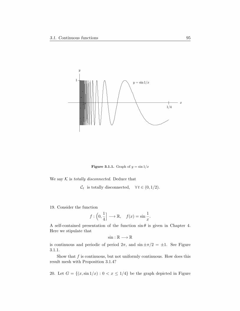
3.1. Continuous functions 95
Figure 3.1.1. Graph of y = sin 1/x
We say K is totally disconnected. Deduce that
Ct is totally disconnected, ∀ t ∈ (0, 1/2).
19. Consider the function
f :(0,
1
4
]−→ R, f(x) = sin
1
x.
A self-contained presentation of the function sin θ is given in Chapter 4.Here we stipulate that
sin : R −→ R
is continuous and periodic of period 2π, and sin±π/2 = ±1. See Figure3.1.1.
Show that f is continuous, but not uniformly continuous. How does thisresult mesh with Proposition 3.1.4?
20. Let G = (x, sin 1/x) : 0 < x ≤ 1/4 be the graph depicted in Figure
96 3. Functions
3.1.1. SetX = G ∪ (0, y) : −1 ≤ y ≤ 1.
Show that X is a compact subset of R2. Show that
X is connected, but not path connected.

3.2. Sequences and series of functions 97
3.2. Sequences and series of functions
Let X and Y be metric spaces, with distance functions dX and dY , respec-tively. Consider a sequence of functions fj : X → Y , which we denote (fj).To say (fj) converges at x to f : X → Y is simply to say that fj(x) → f(x)in Y . If such convergence holds for each x ∈ X, we say (fj) converges to fon X, pointwise.
A stronger type of convergence is uniform convergence. We say fj → funiformly on X provided
(3.2.1) supx∈X
dY (fj(x), f(x)) −→ 0, as j → ∞.
An equivalent characterization is that, for each ε > 0, there exists K ∈ Nsuch that
(3.2.2) j ≥ K =⇒ dY (fj(x), f(x)) ≤ ε, ∀x ∈ X.
A significant property of uniform convergence is that passing to the limitpreserves continuity.
Proposition 3.2.1. If fj : X → Y is continuous for each j and fj → funiformly, then f : X → Y is continuous.
Proof. Fix p ∈ X and take ε > 0. Pick K ∈ N such that (3.2.2) holds.Then pick δ > 0 such that
(3.2.3) x ∈ Bδ(p) =⇒ dY (fK(x), fK(p)) < ε,
which can be done since fK : X → Y is continuous. Together, (3.2.2) and(3.2.3) imply(3.2.4)x ∈ Bδ(p) ⇒ dY (f(x), f(p))
≤ dY (f(x), fK(x)) + dY (fK(x), fK(p)) + dY (fK(p), f(p))
≤ 3ε.
Thus f is continuous at p, for each p ∈ X.
We next consider Cauchy sequences of functions fj : X → Y . To say(fj) is Cauchy at x ∈ X is simply to say (fj(x)) is a Cauchy sequence in Y .We say (fj) is uniformly Cauchy provided
(3.2.5) supx∈X
dY (fj(x), fk(x)) −→ 0, as j, k → ∞.
An equivalent characterization is that, for each ε > 0, there exists K ∈ Nsuch that
(3.2.6) j, k ≥ K =⇒ dY (fj(x), fk(x)) ≤ ε, ∀x ∈ X.

98 3. Functions
If Y is complete, a Cauchy sequence (fj) will have a limit f : X → Y . Wehave the following.
Proposition 3.2.2. Assume Y is complete, and fj : X → Y is uniformlyCauchy. Then (fj) converges uniformly to a limit f : X → Y .
Proof. We have already seen that there exists f : X → Y such that fj(x) →f(x) for each x ∈ X. To finish the proof, take ε > 0, and pick K ∈ N suchthat (3.2.6) holds. Then taking k → ∞ yields
(3.2.7) j ≥ K =⇒ dY (fj(x), f(x)) ≤ ε, ∀x ∈ X,
yielding the uniform convergence.
If, in addition, each fj : X → Y is continuous, we can put Propositions3.2.1 and 3.2.2 together. We leave this to the reader.
It is useful to note the following phenomenon in case, in addition, X iscompact.
Proposition 3.2.3. Assume X is compact, fj : X → Y continuous, andfj → f uniformly on X. Then
(3.2.8) K = f(X) ∪∪j≥1
fj(X) ⊂ Y is compact.
Proof. Let (yν) ⊂ K be an infinite sequence. If there exists j ∈ N suchthat yν ∈ fj(X) for infinitely many ν, convergence of a subsequence to anelement of fj(X) follows from the known compactness of fj(X). Ditto ifyν ∈ f(X) for infinitely many ν. It remains to consider the situation yν ∈fjν (X), jν → ∞ (after perhaps taking a subsequence). That, is, supposeyν = fjν (xν), xν ∈ X, jν → ∞. Passing to a further subsequence, we canassume xν → x in X, and then it follows from the uniform convergence that
(3.2.9) yν −→ y = f(x) ∈ K.
We move from sequences to series. For this, we need some algebraicstructure on Y . Thus, for the rest of this section, we assume
(3.2.10) fj : X −→ Rn,
for some n ∈ N. We look at the infinite series
(3.2.11)
∞∑k=0
fk(x),
3.2. Sequences and series of functions 99
and seek conditions for convergence, which is the same as convergence ofthe sequence of partial sums,
(3.2.12) Sj(x) =
j∑k=0
fk(x).
Parallel to Proposition 1.6.13 of Chapter 1, we have convergence at x ∈ Xprovided
(3.2.13)
∞∑k=0
|fk(x)| <∞,
i.e., provided there exists Bx <∞ such that
(3.2.14)
j∑k=0
|fk(x)| ≤ Bx, ∀ j ∈ N.
In such a case, we say the series (3.2.11) converges absolutely at x. We say(3.2.11) converges uniformly on X if and only if (Sj) converges uniformlyon X. The following sufficient condition for uniform convergence is calledthe Weierstrass M test.
Proposition 3.2.4. Assume there exist Mk such that |fk(x)| ≤Mk, for allx ∈ X, and
(3.2.15)∞∑k=0
Mk <∞.
Then the series (3.2.11) converges uniformly on X, to a limit S : X → Rn.
Proof. This proof is also similar to that of Proposition 1.6.13 of Chapter1, but we review it. We have
(3.2.16)
|Sm+ℓ(x)− Sm(x)| ≤∣∣∣ m+ℓ∑k=m+1
fk(x)∣∣∣
≤m+ℓ∑
k=m+1
|fk(x)|
≤m+ℓ∑
k=m+1
Mk.
Now (3.2.15) implies σm =∑m
k=0Mk is uniformly bounded, so (by Proposi-tion 1.6.11 of Chapter 1), σm β for some β ∈ R+. Hence
(3.2.17) |Sm+ℓ(x)− Sm(x)| ≤ σm+ℓ − σm ≤ β − σm → 0, as m→ ∞,
independent of ℓ ∈ N and x ∈ X. Thus (Sj) is uniformly Cauchy on X, anduniform convergence follows by Propositon 3.2.2.
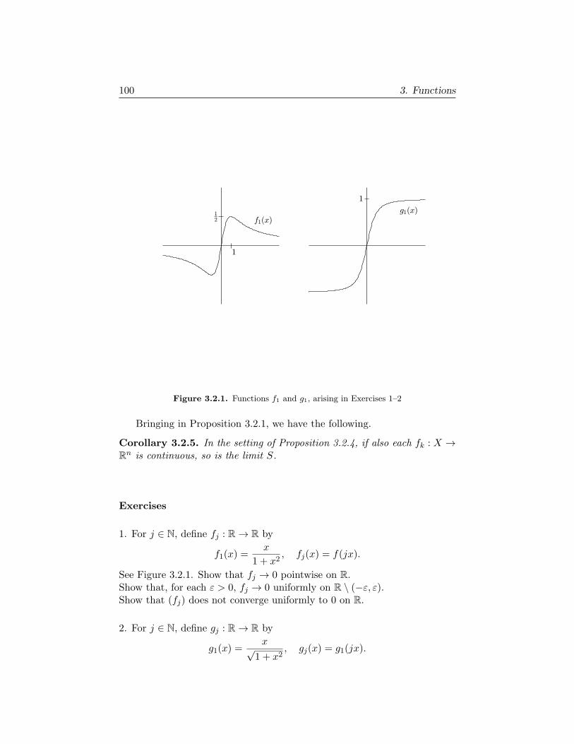
100 3. Functions
Figure 3.2.1. Functions f1 and g1, arising in Exercises 1–2
Bringing in Proposition 3.2.1, we have the following.
Corollary 3.2.5. In the setting of Proposition 3.2.4, if also each fk : X →Rn is continuous, so is the limit S.
Exercises
1. For j ∈ N, define fj : R → R by
f1(x) =x
1 + x2, fj(x) = f(jx).
See Figure 3.2.1. Show that fj → 0 pointwise on R.Show that, for each ε > 0, fj → 0 uniformly on R \ (−ε, ε).Show that (fj) does not converge uniformly to 0 on R.
2. For j ∈ N, define gj : R → R by
g1(x) =x√
1 + x2, gj(x) = g1(jx).

3.2. Sequences and series of functions 101
Show that there exists g : R → R such that gj → g pointwise. Show that gis not continuous on all of R. Where is g discontinuous?
3. Let X be a compact metric space. Assume fj , f : X → R are continuousand
fj(x) f(x), ∀x ∈ X.
Prove that fj → f uniformly on X. (This result is called Dini’s theorem.)Hint. For ε > 0, let Kj(ε) = x ∈ X : f(x) − fj(x) ≥ ε. Note thatKj(ε) ⊃ Kj+1(ε) ⊃ · · · . What about ∩j≥1Kj(ε)?
4. Take gj as in Exercise 2 and consider∞∑k=1
1
k2gk(x).
Show that this series converges uniformly on R, to a continuous limit.
5. Take fj as in Exercise 1 and consider∞∑k=1
1
kfk(x).
Where does this series converge? Where does it converge uniformly? Whereis the sum continuous?Hint. For use in the latter questions, note that, for ℓ ∈ N, ℓ ≤ k ≤ 2ℓ, wehave fk(1/ℓ) ∈ [1/2, 1].
102 3. Functions
3.3. Power series
An important class of infinite series is the class of power series
(3.3.1)∞∑k=0
akzk,
with ak ∈ C. Note that if z1 = 0 and (3.3.1) converges for z = z1, then thereexists C <∞ such that
(3.3.2) |akzk1 | ≤ C, ∀ k.
Hence, if |z| ≤ r|z1|, r < 1, we have
(3.3.3)∞∑k=0
|akzk| ≤ C∞∑k=0
rk =C
1− r<∞,
the last identity being the classical geometric series computation. (Compare(1.10.49) in Chapter 1.) This yields the following.
Proposition 3.3.1. If (3.3.1) converges for some z1 = 0, then either thisseries is absolutely convergent for all z ∈ C, or there is some R ∈ (0,∞)such that the series is absolutely convergent for |z| < R and divergent for|z| > R.
We call R the radius of convergence of (3.3.1). In case of convergencefor all z, we say the radius of convergence is infinite. If R > 0 and (3.1)converges for |z| < R, it defines a function
(3.3.4) f(z) =
∞∑k=0
akzk, z ∈ DR,
on the disk of radius R centered at the origin,
(3.3.5) DR = z ∈ C : |z| < R.
Proposition 3.3.2. If the series (3.3.4) converges in DR, then it convergesuniformly on DS for all S < R, and hence f is continuous on DR, i.e.,given zn, z ∈ DR,
(3.3.6) zn → z =⇒ f(zn) → f(z).
Proof. For each z ∈ DR, there exists S < R such that z ∈ DS , so it sufficesto show that f is continuous on DS whenever 0 < S < R. Pick T such thatS < T < R. We know that there exists C <∞ such that |akT k| ≤ C for allk. Hence
(3.3.7) z ∈ DS =⇒ |akzk| ≤ C(ST
)k.

3.3. Power series 103
Since
(3.3.8)
∞∑k=0
(ST
)k<∞,
the Weierstrass M-test, Proposition 3.2.4, applies, to yield uniform conver-gence on DS . Since
(3.3.9) ∀ k, akzk is continuous,
continuity of f on DS follows from Corollary 3.2.5.
More generally, a power series has the form
(3.3.10) f(z) =∞∑n=0
an(z − z0)n.
It follows from Proposition 3.3.1 that to such a series there is associated aradius of convergence R ∈ [0,∞], with the property that the series convergesabsolutely whenever |z−z0| < R (if R > 0), and diverges whenever |z−z0| >R (if R <∞). We identify R as follows:
(3.3.11)1
R= lim sup
n→∞|an|1/n.
This is established in the following result, which complements Propositions3.3.1–3.3.2.
Proposition 3.3.3. The series (3.3.10) converges whenever |z − z0| < Rand diverges whenever |z− z0| > R, where R is given by (3.3.11). If R > 0,the series converges uniformly on z : |z−z0| ≤ R′, for each R′ < R. Thus,when R > 0, the series (3.3.10) defines a continuous function
(3.3.12) f : DR(z0) −→ C,
where
(3.3.13) DR(z0) = z ∈ C : |z − z0| < R.
Proof. If R′ < R, then there exists N ∈ Z+ such that
n ≥ N =⇒ |an|1/n <1
R′ =⇒ |an|(R′)n < 1.
Thus
(3.3.14) |z − z0| < R′ < R =⇒ |an(z − z0)n| ≤
∣∣∣z − z0R′
∣∣∣n,for n ≥ N , so (3.3.10) is dominated by a convergent geometrical series inDR′(z0).

104 3. Functions
For the converse, we argue as follows. Suppose R′′ > R, so infinitelymany |an|1/n ≥ 1/R′′, hence infinitely many |an|(R′′)n ≥ 1. Then
|z − z0| ≥ R′′ > R =⇒ infinitely many |an(z − z0)n| ≥
∣∣∣z − z0R′′
∣∣∣n ≥ 1,
forcing divergence for |z − z0| > R.
The assertions about uniform convergence and continuity follow as inProposition 3.3.2.
It is useful to note that we can multiply power series with radius ofconvergence R > 0. In fact, there is the following more general result onproducts of absolutely convergent series.
Proposition 3.3.4. Given absolutely convergent series
(3.3.15) A =
∞∑n=0
αn, B =
∞∑n=0
βn,
we have the absolutely convergent series
(3.3.16) AB =
∞∑n=0
γn, γn =
n∑j=0
αjβn−j .
Proof. Take Ak =∑k
n=0 αn, Bk =∑k
n=0 βn. Then
(3.3.17) AkBk =k∑
n=0
γn +Rk
with(3.3.18)
Rk =∑
(m,n)∈σ(k)
αmβn, σ(k) = (m,n) ∈ Z+ × Z+ : m,n ≤ k,m+ n > k.
Hence
(3.3.19)
|Rk| ≤∑
m≤k/2
∑k/2≤n≤k
|αm| |βn|+∑
k/2≤m≤k
∑n≤k
|αm| |βn|
≤ A∑
n≥k/2
|βn|+B∑
m≥k/2
|αm|,
where
(3.3.20) A =
∞∑n=0
|αn| <∞, B =
∞∑n=0
|βn| <∞.
It follows that Rk → 0 as k → ∞. Thus the left side of (3.17) convergesto AB and the right side to
∑∞n=0 γn. The absolute convergence of (3.3.16)
3.3. Power series 105
follows by applying the same argument with αn replaced by |αn| and βnreplaced by |βn|.
Corollary 3.3.5. Suppose the following power series converge for |z| < R:
(3.3.21) f(z) =∞∑n=0
anzn, g(z) =
∞∑n=0
bnzn.
Then, for |z| < R,
(3.3.22) f(z)g(z) =
∞∑n=0
cnzn, cn =
n∑j=0
ajbn−j .
The following result, which is related to Proposition 3.3.4, has a similarproof. (For still more along these lines, see §3.5.)
Proposition 3.3.6. If ajk ∈ C and∑
j,k |ajk| < ∞, then∑
j ajk is ab-
solutely convergent for each k,∑
k ajk is absolutely convergent for each j,and
(3.3.23)∞∑j=0
( ∞∑k=0
ajk
)=
∞∑k=0
( ∞∑j=0
ajk
)=
∑j,k
ajk.
Proof. Clearly the hypothesis implies∑
j |ajk| < ∞ for each k, and also∑k |ajk| <∞ for each j. It also implies that there exists B <∞ such that
SN =
N∑j=0
N∑k=0
|ajk| ≤ B, ∀N.
Now SN is bounded and monotone, so there exists a limit, SN A <∞ asN ∞. It follows that, for each ε > 0, there exists N ∈ N such that∑
(j,k)∈C(N)
|ajk| < ε, C(N) = (j, k) ∈ N× N : j > N or k > N.
Note that if M,K ≥ N , then∣∣∣ M∑j=0
( K∑k=0
ajk
)−
N∑j=0
N∑k=0
ajk
∣∣∣ ≤ ∑(j,k)∈C(N)
|ajk|,
hence ∣∣∣ M∑j=0
( ∞∑k=0
ajk
)−
N∑j=0
N∑k=0
ajk
∣∣∣ ≤ ∑(j,k)∈C(N)
|ajk|.
Therefore ∣∣∣ ∞∑j=0
( ∞∑k=0
ajk
)−
N∑j=0
N∑k=0
ajk
∣∣∣ ≤ ∑(j,k)∈C(N)
|ajk|.

106 3. Functions
We have a similar result with the roles of j and k reversed, and clearly thetwo finite sums agree. It follows that∣∣∣ ∞∑
j=0
( ∞∑k=0
ajk
)−
∞∑k=0
( ∞∑j=0
ajk
)∣∣∣ < 2ε, ∀ ε > 0,
yielding (3.3.23).
Using Proposition 3.3.6, we demonstrate the following. (Thanks toShrawan Kumar for this argument.)
Proposition 3.3.7. If (3.3.10) has a radius of convergence R > 0, andz1 ∈ DR(z0), then f(z) has a convergent power series about z1:
(3.3.24) f(z) =
∞∑k=0
bk(z − z1)k, for |z − z1| < R− |z1 − z0|.
Proof. There is no loss in generality in taking z0 = 0, which we will dohere, for notational simplicity. Setting fz1(ζ) = f(z1 + ζ), we have from(3.3.10)
(3.3.25)
fz1(ζ) =
∞∑n=0
an(ζ + z1)n
=
∞∑n=0
n∑k=0
an
(n
k
)ζkzn−k
1 ,
the second identity by the binomial formula. Now,
(3.3.26)∞∑n=0
n∑k=0
|an|(n
k
)|ζ|k|z1|n−k =
∞∑n=0
|an|(|ζ|+ |z1|)n <∞,
provided |ζ| + |z1| < R, which is the hypothesis in (3.3.24) (with z0 = 0).Hence Proposition 3.3.6 gives
(3.3.27) fz1(ζ) =
∞∑k=0
( ∞∑n=k
an
(n
k
)zn−k1
)ζk.
Hence (3.3.2) holds, with
(3.3.28) bk =
∞∑n=k
an
(n
k
)zn−k1 .
This proves Proposition 3.3.7. Note in particular that
(3.3.29) b1 =∞∑n=1
nanzn−11 .
3.3. Power series 107
For more on power series, see §4.3 of Chapter 4.
Exercises
1. Let ak ∈ C. Assume there exist K ∈ N, α < 1 such that
(3.3.30) k ≥ K =⇒∣∣∣ak+1
ak
∣∣∣ ≤ α.
Show that∑∞
k=0 ak is absolutely convergent.Note. This is the ratio test.
2. Determine the radius of convergence R for each of the following powerseries. If 0 < R <∞, try to determine when convergence holds at points on|z| = R.
(3.3.31)
∞∑n=0
zn,∞∑n=1
zn
n,
∞∑n=1
zn
n2,
∞∑n=1
zn
n!,
∞∑n=1
zn
2n,
∞∑n=1
z2n
2n,
∞∑n=1
nzn,∞∑n=1
n2zn,∞∑n=1
n! zn.
3. Prove Proposition 3.3.6.
4. We have seen that
(3.3.32)1
1− z=
∞∑k=0
zk, |z| < 1.
Find power series in z for
(3.3.33)1
z − 2,
1
z + 3.
Where do they converge?
5. Use Corollary 3.3.5 to produce a power series in z for
(3.3.34)1
z2 + z − 6.
Where does the series converge?

108 3. Functions
6. As an alternative to the use of Corollary 3.3.5, write (3.3.34) as a linearcombination of the functions (3.3.33).
7. Find the power series on z for
1
1 + z2.
Hint. Replace z by −z2 in (3.3.32).
8. Given a > 0, find the power series in z for
1
a2 + z2.
3.4. Spaces of functions
If X and Y are metric spaces, the space C(X,Y ) of continuous maps f :X → Y has a natural metric structure, under some additional hypotheses.We use
(3.4.1) D(f, g) = supx∈X
d(f(x), g(x)
).
This sup exists provided f(X) and g(X) are bounded subsets of Y, where tosay B ⊂ Y is bounded is to say d : B ×B → [0,∞) has bounded image. Inparticular, this supremum exists if X is compact.
Proposition 3.4.1. If X is a compact metric space and Y is a completemetric space, then C(X,Y ), with the metric (3.4.1), is complete.
Proof. ThatD(f, g) satisfies the conditions to define a metric on C(X,Y ) isstraightforward. We check completeness. Suppose (fν) is a Cauchy sequencein C(X,Y ), so, as ν → ∞,
(3.4.2) supk≥0
supx∈X
d(fν+k(x), fν(x)
)≤ εν → 0.
Then in particular (fν(x)) is a Cauchy sequence in Y for each x ∈ X, so itconverges, say to g(x) ∈ Y . It remains to show that g ∈ C(X,Y ) and thatfν → g in the metric (3.4.1).
In fact, taking k → ∞ in the estimate above, we have
(3.4.3) supx∈X
d(g(x), fν(x)
)≤ εν → 0,
i.e., fν → g uniformly. It remains only to show that g is continuous. Forthis, let xj → x in X and fix ε > 0. Pick N so that εN < ε. Since fN is
3.4. Spaces of functions 109
continuous, there exists J such that j ≥ J ⇒ d(fN (xj), fN (x)) < ε. Hence
j ≥ J ⇒ d(g(xj), g(x)
)≤ d
(g(xj), fN (xj)
)+ d
(fN (xj), fN (x)
)+ d
(fN (x), g(x)
)< 3ε.
This completes the proof.
In case Y = R, we write C(X,R) = C(X). The distance function (3.4.1)can then be written
(3.4.4) D(f, g) = ∥f − g∥sup, ∥f∥sup = supx∈X
|f(x)|.
∥f∥sup is a norm on C(X).
Generally, a norm on a vector space V is an assignment f 7→ ∥f∥ ∈[0,∞), satisfying
(3.4.5) ∥f∥ = 0 ⇔ f = 0, ∥af∥ = |a| ∥f∥, ∥f + g∥ ≤ ∥f∥+ ∥g∥,given f, g ∈ V and a a scalar (in R or C). A vector space equipped witha norm is called a normed vector space. It is then a metric space, withdistance function D(f, g) = ∥f − g∥. If the space is complete, one calls V aBanach space.
In particular, by Proposition 3.4.1, C(X) is a Banach space, when X isa compact metric space.
The next result is a special case of the Arzela-Ascoli Theorem. To stateit, we say a modulus of continuity is a strictly monotonically increasing,continuous function ω : [0,∞) → [0,∞) such that ω(0) = 0.
Proposition 3.4.2. Let X and Y be compact metric spaces, and fix a mod-ulus of continuity ω(δ). Then
(3.4.6) Cω =f ∈ C(X,Y ) : d
(f(x), f(x′)
)≤ ω
(d(x, x′)
)∀x, x′ ∈ X
is a compact subset of C(X,Y ).
Proof. Let (fν) be a sequence in Cω. Let Σ be a countable dense subsetof X, as in Corollary 2.3.2 of Chapter 2. For each x ∈ Σ, (fν(x)) is asequence in Y, which hence has a convergent subsequence. Using a diagonalconstruction similar to that in the proof of Proposition 2.3.10 of Chapter 2,we obtain a subsequence (φν) of (fν) with the property that φν(x) convergesin Y, for each x ∈ Σ, say
(3.4.7) φν(x) → ψ(x),
for all x ∈ Σ, where ψ : Σ → Y.
So far, we have not used (3.4.6). This hypothesis will now be used toshow that φν converges uniformly on X. Pick ε > 0. Then pick δ > 0 suchthat ω(δ) < ε/3. Since X is compact, we can cover X by finitely many balls
110 3. Functions
Bδ(xj), 1 ≤ j ≤ N, xj ∈ Σ. Pick M so large that φν(xj) is within ε/3 ofits limit for all ν ≥ M (when 1 ≤ j ≤ N). Now, for any x ∈ X, pickingℓ ∈ 1, . . . , N such that d(x, xℓ) ≤ δ, we have, for k ≥ 0, ν ≥M,
(3.4.8)
d(φν+k(x), φν(x)
)≤ d
(φν+k(x), φν+k(xℓ)
)+ d
(φν+k(xℓ), φν(xℓ)
)+ d
(φν(xℓ), φν(x)
)≤ ε/3 + ε/3 + ε/3.
Thus (φν(x)) is Cauchy in Y for all x ∈ X, hence convergent. Call the limitψ(x), so we now have (3.4.7) for all x ∈ X. Letting k → ∞ in (3.4.8) wehave uniform convergence of φν to ψ. Finally, passing to the limit ν → ∞in
(3.4.9) d(φν(x), φν(x′)) ≤ ω(d(x, x′))
gives ψ ∈ Cω.
We want to re-state Proposition 3.4.2, bringing in the notion of equicon-tinuity. Given metric spaces X and Y , and a set of maps F ⊂ C(X,Y ), wesay F is equicontinuous at a point x0 ∈ X provided
(3.4.10)∀ ε > 0, ∃ δ > 0 such that ∀x ∈ X, f ∈ F ,dX(x, x0) < δ =⇒ dY (f(x), f(x0)) < ε.
We say F is equicontinuous on X if it is equicontinuous at each point of X.We say F is uniformly equicontinuous on X provided
(3.4.11)∀ ε > 0, ∃ δ > 0 such that ∀x, x′ ∈ X, f ∈ F ,dX(x, x′) < δ =⇒ dY (f(x), f(x
′)) < ε.
Note that (3.4.11) is equivalent to the existence of a modulus of continuityω such that F ⊂ Cω, given by (3.4.6). It is useful to record the followingresult.
Proposition 3.4.3. Let X and Y be metric spaces, F ⊂ C(X,Y ). AssumeX is compact. then
(3.4.12) F equicontinuous =⇒ F is uniformly equicontinuous.
Proof. The argument is a variant of the proof of Proposition 3.1.4. Inmore detail, suppose there exist xν , x
′ν ∈ X, ε > 0, and fν ∈ F such that
d(xν , x′ν) ≤ 2−ν but
(3.4.13) d(fν(xν), fν(x′ν)) ≥ ε.
Taking a convergent subsequence xνj → p ∈ X, we also have x′νj → p. Now
equicontinuity of F at p implies that there exists N <∞ such that
(3.4.14) d(g(xνj ), g(p)) <ε
2, ∀ j ≥ N, g ∈ F ,

3.4. Spaces of functions 111
contradicting (3.4.13).
Putting together Propositions 3.4.2 and 3.4.3 then gives the following.
Proposition 3.4.4. Let X and Y be compact metric spaces. If F ⊂C(X,Y ) is equicontinuous on X, then it has compact closure in C(X,Y ).
Exercises
1. Let X and Y be compact metric spaces. Show that if F ⊂ C(X,Y )is compact, then F is equicontinuous. (This is a converse to Proposition3.4.4.)
2. Let X be a compact metric space, and r ∈ (0, 1]. Define Lipr(X,Rn)to consist of continuous functions f : X → Rn such that, for some L < ∞(depending on f),
|f(x)− f(y)| ≤ LdX(x, y)r, ∀x, y ∈ X.
Define a norm
∥f∥r = supx∈X
|f(x)|+ supx,y∈X,x =y
|f(x)− f(y)|d(x, y)r
.
Show that Lipr(X,Rn) is a complete metric space, with distance functionDr(f, g) = ∥f − g∥r.
3. In the setting of Exercise 2, show that if 0 < r < s ≤ 1 and f ∈Lips(X,Rn), then
∥f∥r ≤ C∥f∥1−θsup ∥f∥θs, θ =
r
s∈ (0, 1).
4. In the setting of Exercise 2, show that if 0 < r < s ≤ 1, then
f ∈ Lips(X,Rn) : ∥f∥s ≤ 1
is compact in Lipr(X,Rn).
5. Let X be a compact metric space, and define C(X) as in (3.4.4). Take
P : C(X)× C(X) −→ C(X), P (f, g)(x) = f(x)g(x).
Show that P is continuous.
112 3. Functions
3.5. Absolutely convergent series
Here we look at results on infinite series of numbers (or vectors), related tomaterial in Sections 3.2 and 3.3. We concentrate on absolutely convergentseries. Rather than looking at a series as a sum of ak for k ∈ N, we find itconvenient to consider the following setting. Let Z be a countably infiniteset, and take a function
(3.5.1) f : Z −→ Rn.
We say f is absolutely summable, and write f ∈ ℓ1(Z,Rn), provided thereexists M <∞ such that
(3.5.2)∑k∈F
|f(k)| ≤M, for each finite set F ⊂ Z.
In notation used in §§3.2–3.3, we would have f(k) denoted by fk, k ∈ N (ormaybe k ∈ Z+), but we use the notation f(k) here. If f ∈ ℓ1(Z,Rn), we saythe series
(3.5.3)∑k∈Z
f(k) is absolutely convergent.
Also we would like to write the characterization (3.5.2) as
(3.5.4)∑k∈Z
|f(k)| <∞.
Of course, implicit in (3.5.3)–(3.5.4) is that∑
k∈Z f(k) and∑
k∈Z |f(k)| arewell defined elements of Rn and [0,∞), respectively. We will see shortly thatthis is the case.
To start, we note that, by hypothesis (3.5.2), if f ∈ ℓ1(Z,Rn), the quan-tity
(3.5.5) M(f) = sup∑k∈F
|f(k)| : F ⊂ Z finite
is well defined, and M(f) ≤ M . Hence, given ε > 0, there is a finite setKε(f) ⊂ Z such that
(3.5.6)∑
k∈Kε(f)
|f(k)| ≥M(f)− ε.
These observations yield the following.
Proposition 3.5.1. If f ∈ ℓ1(Z,Rn), then
(3.5.7) F ⊂ Z \Kε(f) finite =⇒∑k∈F
|f(k)| ≤ ε.
This leads to:
3.5. Absolutely convergent series 113
Corollary 3.5.2. If f ∈ ℓ1(Z,Rn) and A,B ⊃ Kε(f) are finite, then
(3.5.8)∣∣∣∑k∈A
f(k)−∑k∈B
f(k)∣∣∣ ≤ 2ε.
To proceed, we bring in the following notion. Given subsets Fν ⊂ Z(ν ∈ N), we say Fν → Z provided that, if F ⊂ Z is finite, there existsN = N(F ) < ∞ such that ν ≥ N ⇒ Fν ⊃ F . Since Z is countable, we seethat there exist sequences Fν → Z such that each Fν is finite.
Proposition 3.5.3. Take f ∈ ℓ1(Z,Rn). Assume Fν ⊂ Z are finite andFν → Z. Then there exists SZ(f) ∈ Rn such that
(3.5.9) limν→∞
∑k∈Fν
f(k) = SZ(f).
Furthermore, the limit SZ(f) is independent of the choice of finite Fν → Z.
Proof. By Corollary 3.5.2, the sequence Sν(f) =∑
k∈Fνf(k) is a Cauchy
sequence in Rn, so it converges to a limit we call SZ(f). As for the inde-pendence of the choice, note that if also F ′
ν are finite and F ′ν → Z, we can
interlace Fν and F ′ν .
Given Proposition 3.5.3, we set
(3.5.10)∑k∈Z
f(k) = SZ(f), for f ∈ ℓ1(Z,Rn).
Note in particular that, if f ∈ ℓ1(Z,Rn), then |f | ∈ ℓ1(Z,R), and
(3.5.11)∑k∈Z
|f(k)| =M(f),
defined in (3.5.6). (These two results illuminate (3.5.3)–(3.5.4).)
Remark. Proposition 3.5.3 contains Propositions 1.6.13 and 1.10.3 of Chap-ter 1. It is stronger than those results, in that it makes clear that the orderof summation is irrelevant.
Our next goal is to establish the following result, known as a dominatedconvergence theorem.
Proposition 3.5.4. For ν ∈ N, let fν ∈ ℓ1(Z,Rn), and let g ∈ ℓ1(Z,R).Assume
(3.5.12) |fν(k)| ≤ g(k), ∀ ν ∈ N, k ∈ Z,
and
(3.5.13) limν→∞
fν(k) = f(k), ∀ k ∈ Z.

114 3. Functions
Then f ∈ ℓ1(Z,Rn) and
(3.5.14) limν→∞
∑k∈Z
fν(k) =∑k∈Z
f(k).
Proof. We have∑
k∈Z |g(k)| =∑
k∈Z g(k) = M < ∞. Parallel to (3.5.6)–(3.5.7), for each ε > 0, we can take a finite set Kε(g) ⊂ Z such that∑
k∈Kε(g)g(k) ≥M − ε, and hence
(3.5.15)
F ⊂ Z \Kε(g) finite =⇒∑k∈F
g(k) ≤ ε
=⇒∑k∈F
|fν(k)| ≤ ε, ∀ ν ∈ N,
the last implication by (3.5.12). In light of Proposition 3.5.3, we can restatethis conclusion as
(3.5.16)∑
k∈Z\Kε(g)
|fν(k)| ≤ ε, ∀ ν ∈ N.
Bringing in (3.5.13), we also have
(3.5.17)∑k∈F
|f(k)| ≤ ε, for each finite F ⊂ Z \Kε(g),
and hence
(3.5.18)∑
k∈Z\Kε(g)
|f(k)| ≤ ε.
On the other hand, since Kε(g) is finite,
(3.5.19) limν→∞
∑k∈Kε(g)
fν(k) =∑
k∈Kε(g)
f(k).
It follows that
(3.5.20)
lim supν→∞
|SZ(fν)− SZ(f)|
≤ lim supν→∞
|SKε(g)(fν)− SKε(g)(f)|
+ lim supν→∞
|SZ\Kε(g)(fν)− SZ\Kε(g)(f)|
≤ 2ε,
for each ε > 0, hence
(3.5.21) lim supν→∞
|SZ(fν)− SZ(f)| = 0,
which is equivalent to (3.5.14).
Here is one simple but basic application of Proposition 3.5.4.

3.5. Absolutely convergent series 115
Corollary 3.5.5. Assume f ∈ ℓ1(Z,Rn). For ν ∈ N, let Fν ⊂ Z andassume Fν → Z. One need not assume that Fν is finite. Then
(3.5.22) limν→∞
∑k∈Fν
f(k) =∑k∈Z
f(k).
Proof. Apply Proposition 3.5.4 with g(k) = |f(k)| and fν(k) = χFν (k)f(k).
The following result recovers Proposition 3.3.6.
Proposition 3.5.6. Let Y and Z be countable sets, and assume f ∈ ℓ1(Y ×Z,Rn), so
(3.5.23)∑
(j,k)∈Y×Z
|f(j, k)| =M <∞.
Then, for each j ∈ Y ,
(3.5.24)∑k∈Z
f(j, k) = g(j)
is absolutely convergent,
(3.5.25) g ∈ ℓ1(Y,Rn),
and
(3.5.26)∑
(j,k)∈Y×Z
f(j, k) =∑j∈Y
g(j).
hence
(3.5.27)∑
(j,k)∈Y×Z
f(j, k) =∑j∈Y
(∑k∈Z
f(j, k)).
Proof. Since∑
k∈Z |f(j, k)| is dominated by (3.5.23), the absolute conver-gence in (3.5.24) is clear. Next, if A ⊂ Y is finite, then
(3.5.28)∑j∈A
|g(j)| ≤∑j∈A
∑k∈Z
|f(j, k)| ≤M,
so g ∈ ℓ1(Y,Rn). Furthermore, if Aν ⊂ Y are finite, then
(3.5.29)∑j∈Aν
g(j) =∑
(j,k)∈Fν
f(j, k), Fν = Aν × Z,
and Aν → Y ⇒ Fν → Y × Z, so (3.5.26) follows from Corollary 3.5.5.
We next examine implications for multiplying two absolutely convergentseries, extending Proposition 3.3.4.
116 3. Functions
Proposition 3.5.7. Let Y and Z be countable sets, and assume f ∈ ℓ1(Y,C),g ∈ ℓ1(Z,C). Define
(3.5.30) f × g : Y × Z −→ C, (f × g)(j, k) = f(j)g(k).
Then
(3.5.31) f × g ∈ ℓ1(Y × Z,C).
Proof. Given a finite set F ⊂ Y × Z, there exist finite A ⊂ Y and B ⊂ Zsuch that F ⊂ A×B. Then
(3.5.32)
∑(j,k)∈F
|f(j)g(k)| ≤∑
(j,k)∈A×B
|f(j)g(k)|
=∑j∈A
|f(j)|∑k∈B
|g(k)|
≤M(f)M(g),
where M(f) =∑
j∈Y |f(j)| and M(g) =∑
k∈Z |g(k)|.
We can apply Proposition 3.5.6 to f × g to deduce:
Proposition 3.5.8. In the setting of Proposition 3.5.7,
(3.5.33)∑
(j,k)∈Y×Z
f(j)g(k) =(∑j∈Y
f(j))(∑
k∈Zg(k)
).
In case Y = Z = N, we can then apply Proposition 3.5.3, with Z replacedby N× N, f replaced by f × g, and
(3.5.34) Fν = (j, k) ∈ N× N : j + k ≤ ν,and recover Proposition 3.3.4, including (3.3.16).
Chapter 4
Calculus
Having foundational material on numbers, spaces, and functions, we proceedfurther into the heart of analysis, with a rigorous development of calculus,for functions of one real variable.
Section 4.1 introduces the derivative, establishes basic identities like theproduct rule and the chain rule, and also obtains some important theoreticalresults, such as the Mean Value Theorem and the Inverse Function Theorem.One application of the latter is the study of x1/n, for x > 0, which leadsmore generally to xr, for x > 0 and r ∈ Q.
Section 4.2 brings in the integral, more precisely the Riemann integral.A major result is the Fundamental Theorem of Calculus, whose proof makesessential use of the Mean Value Theorem. Another topic is the change ofvariable formula for integrals (treated in some exercises).
In §4.3 we treat power series, continuing the development from §3.3 ofChapter 3. Here we treat such topics as term by term differentiation of powerseries, and formulas for the remainder when a power series is truncated. Anapplication of such remainder formulas is made to the study of convergenceof the power series about x = 0 of (1− x)b.
Section 4.4 studies curves in Euclidean space Rn, with particular atten-tion to arc length. We derive an integral formula for arc length. We showthat a smooth curve can be reparametrized by arc length, as an applicationof the Inverse Function Theorem. We then take a look at the unit circle S1
in R2. Using the parametrization of part of S1 as (t,√1− t2), we obtain
a power series for arc lengths, as an application of material of §3 on powerseries of (1 − x)b, with b = −1/2, and x replaced by t2. We also bring in
117
118 4. Calculus
the trigonometric functions, having the property that (cos t, sin t) providesa parametrization of S1 by arc length.
Section 4.5 goes much further into the study of the trigonometric func-tions. Actually, it begins with a treatment of the exponential function et,observes that such treatment extends readily to eat, given a ∈ C, and thenestablishes that eit provides a unit speed parametrization of S1. This di-rectly gives Euler’s formula
eit = cos t+ i sin t,
and provides for a unified treatment of the exponential and trigonometricfunctions. We also bring in log as the inverse function to the exponential,and we use the formula xr = er log x to generalize results of §4.1 on xr fromr ∈ Q to r ∈ R, and further, to r ∈ C.
In §4.6 we give a natural extension of the Riemann integral from theclass of bounded (Riemann integrable) functions to a class of unbounded“integrable” functions. The treatment here is perhaps a desirable alternativeto discussions one sees of “improper integrals.”
4.1. The derivative 119
4.1. The derivative
Consider a function f , defined on an interval (a, b) ⊂ R, taking values in Ror C. Given x ∈ (a, b), we say f is differentiable at x, with derivative f ′(x),provided
(4.1.1) limh→0
f(x+ h)− f(x)
h= f ′(x).
We also use the notation
(4.1.2)df
dx(x) = f ′(x).
A characterization equivalent to (4.1.1) is
(4.1.3) f(x+ h) = f(x) + f ′(x)h+ r(x, h), r(x, h) = o(h),
where
(4.1.4) r(x, h) = o(h) meansr(x, h)
h→ 0 as h→ 0.
Clearly if f is differentiable at x then it is continuous at x. We say f isdifferentiable on (a, b) provided it is differentiable at each point of (a, b). Ifalso g is defined on (a, b) and differentiable at x, we have
(4.1.5)d
dx(f + g)(x) = f ′(x) + g′(x).
We also have the following product rule:
(4.1.6)d
dx(fg)(x) = f ′(x)g(x) + f(x)g′(x).
To prove (4.1.6), note that
f(x+ h)g(x+ h)− f(x)g(x)
h
=f(x+ h)− f(x)
hg(x) + f(x+ h)
g(x+ h)− g(x)
h.
We can use the product rule to show inductively that
(4.1.7)d
dxxn = nxn−1,
for all n ∈ N. In fact, this is immediate from (4.1.1) if n = 1. Given that itholds for n = k, we have
d
dxxk+1 =
d
dx(xxk) =
dx
dxxk + x
d
dxxk
= xk + kxk
= (k + 1)xk,
120 4. Calculus
completing the induction. We also have
1
h
( 1
x+ h− 1
x
)= − 1
x(x+ h)→ − 1
x2, as h→ 0,
for x = 0, hence
(4.1.8)d
dx
1
x= − 1
x2, if x = 0.
From here, we can extend (4.1.7) from n ∈ N to all n ∈ Z (requiring x = 0if n < 0).
A similar inductive argument yields
(4.1.9)d
dxf(x)n = nf(x)n−1f ′(x),
for n ∈ N, and more generally for n ∈ Z (requiring f(x) = 0 if n < 0).
Going further, we have the following chain rule. Suppose f : (a, b) →(α, β) is differentiable at x and g : (α, β) → R (or C) is differentiable aty = f(x). Form G = g f , i.e., G(x) = g(f(x)). We claim
(4.1.10) G = g f =⇒ G′(x) = g′(f(x))f ′(x).
To see this, write
(4.1.11)
G(x+ h) = g(f(x+ h))
= g(f(x) + f ′(x)h+ rf (x, h))
= g(f(x)) + g′(f(x))(f ′(x)h+ rf (x, h))
+ rg(f(x), f′(x)h+ rf (x, h)).
Here,
rf (x, h)
h−→ 0 as h→ 0,
and alsorg(f(x), f
′(x)h+ rf (x, h))
h−→ 0, as h→ 0,
so the analogue of (4.1.3) applies.
The derivative has the following important connection to maxima andminima.
Proposition 4.1.1. Let f : (a, b) → R. Suppose x ∈ (a, b) and
(4.1.12) f(x) ≥ f(y), ∀ y ∈ (a, b).
If f is differentiable at x, then f ′(x) = 0. The same conclusion holds iff(x) ≤ f(y) for all y ∈ (a, b).
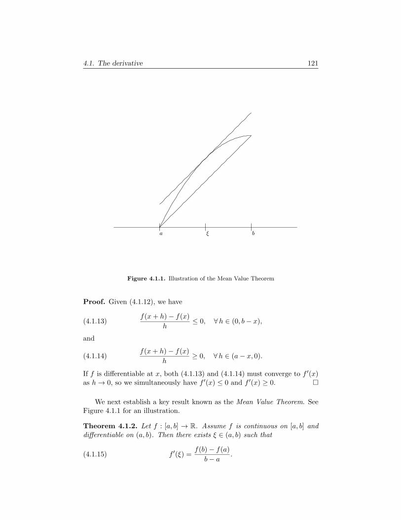
4.1. The derivative 121
Figure 4.1.1. Illustration of the Mean Value Theorem
Proof. Given (4.1.12), we have
(4.1.13)f(x+ h)− f(x)
h≤ 0, ∀h ∈ (0, b− x),
and
(4.1.14)f(x+ h)− f(x)
h≥ 0, ∀h ∈ (a− x, 0).
If f is differentiable at x, both (4.1.13) and (4.1.14) must converge to f ′(x)as h→ 0, so we simultaneously have f ′(x) ≤ 0 and f ′(x) ≥ 0.
We next establish a key result known as the Mean Value Theorem. SeeFigure 4.1.1 for an illustration.
Theorem 4.1.2. Let f : [a, b] → R. Assume f is continuous on [a, b] anddifferentiable on (a, b). Then there exists ξ ∈ (a, b) such that
(4.1.15) f ′(ξ) =f(b)− f(a)
b− a.

122 4. Calculus
Proof. Let g(x) = f(x)−κ(x−a), where κ denotes the right side of (4.1.15).Then g(a) = g(b). The result (4.1.15) is equivalent to the assertion that
(4.1.16) g′(ξ) = 0
for some ξ ∈ (a, b). Now g is continuous on the compact set [a, b], so itassumes both a maximum and a minimum on this set. If g has a maximumat a point ξ ∈ (a, b), then (4.1.16) follows from Proposition 4.1.1. If not,the maximum must be g(a) = g(b), and then g must assume a minimum atsome point ξ ∈ (a, b). Again Proposition 4.1.1 implies (4.1.16).
We use the Mean Value Theorem to produce a criterion for constructingthe inverse of a function. Let
(4.1.17) f : [a, b] −→ R, f(a) = α, f(b) = β.
Assume f is continuous on [a, b], differentiable on (a, b), and
(4.1.18) 0 < γ0 ≤ f ′(x) ≤ γ1 <∞, ∀x ∈ (a, b).
Then (4.1.15) implies
(4.1.19) γ0(b− a) ≤ β − α ≤ γ1(b− a).
We can also apply Theorem 4.1.2 to f , restricted to an interval [x1, x2] ⊂[a, b], to get
(4.1.20) γ0(x2 − x1) ≤ f(x2)− f(x1) ≤ γ1(x2 − x1), if a ≤ x1 < x2 ≤ b.
It follows that
(4.1.21) f : [a, b] −→ [α, β] is one-to-one.
The intermediate value theorem implies f : [a, b] → [α, β] is onto. Conse-quently f has an inverse
(4.1.22) g : [α, β] −→ [a, b], g(f(x)) = x, f(g(y)) = y,
and (4.1.20) implies(4.1.23)γ0(g(y2)− g(y1)) ≤ y2 − y1 ≤ γ1(g(y2)− g(y1)), if α ≤ y1 < y2 ≤ β.
The following result is known as the Inverse Function Theorem.
Theorem 4.1.3. If f is continuous on [a, b] and differentiable on (a, b),and (1.17)–(1.18) hold, then its inverse g : [α, β] → [a, b] is differentiable on(α, β), and
(4.1.24) g′(y) =1
f ′(x), for y = f(x) ∈ (α, β).
The same conclusion holds if in place of (1.18) we have
(4.1.25) −γ1 ≤ f ′(x) ≤ −γ0 < 0, ∀x ∈ (a, b),
except that then β < α.
4.1. The derivative 123
Proof. Fix y ∈ (α, β), and let x = g(y), so y = f(x). From (4.1.22) wehave, for h small enough,
x+ h = g(f(x+ h)) = g(f(x) + f ′(x)h+ r(x, h)),
i.e.,
(4.1.26) g(y + f ′(x)h+ r(x, h)) = g(y) + h, r(x, h) = o(h).
Now (4.1.23) implies
(4.1.27) |g(y1 + r(x, h))− g(y1)| ≤1
γ0|r(x, h)|,
provided y1, y1 + r(y, h) ∈ [α, β], so, with h = f ′(x)h, and y1 = y + h, wehave
(4.1.28) g(y + h) = g(y) +h
f ′(x)+ o(h),
yielding (4.1.24) from the analogue of (4.1.3).
Remark. If one knew that g were differentiable, as well as f , then the iden-tity (4.1.24) would follow by differentiating g(f(x)) = x, applying the chainrule. However, an additional argument, such as given above, is necessary toguarantee that g is differentiable.
Theorem 4.1.3 applies to the functions
(4.1.29) pn(x) = xn, n ∈ N.
By (4.1.7), p′n(x) > 0 for x > 0, so (4.1.18) holds when 0 < a < b <∞. Wecan take a 0 and b ∞ and see that
(4.1.30) pn : (0,∞) −→ (0,∞) is invertible,
with differentiable inverse qn : (0,∞) → (0,∞). We use the notation
(4.1.31) x1/n = qn(x), x > 0,
so, given n ∈ N,
(4.1.32) x > 0 =⇒ x = x1/n · · ·x1/n, (n factors).
Note. We recall that x1/n was constructed, for x > 0, in Chapter 1, §1.7,and its continuity discussed in Chapter 3, §3.1.
Given m ∈ Z, we can set
(4.1.33) xm/n = (x1/n)m, x > 0,

124 4. Calculus
and verify that (x1/kn)km = (x1/n)m. Thus we have xr defined for all r ∈ Q,when x > 0. We have
(4.1.34) xr+s = xrxs, for x > 0, r, s ∈ Q.
See Exercises 3–5 in §1.7 of Chapter 1. Applying (4.1.24) to f(x) = xn and
g(y) = y1/n, we have
(4.1.35)d
dyy1/n =
1
nxn−1, y = xn, x > 0.
Now xn−1 = y/x = y1−1/n, so we get
(4.1.36)d
dyyr = ryr−1, y > 0,
when r = 1/n. Putting this together with (4.1.9) (with m in place of n), weget (4.1.36) for all r = m/n ∈ Q.
The definition of xr for x > 0 and the identity (4.1.36) can be extendedto all r ∈ R, with some more work. We will find a neat way to do this in§4.5.
We recall another common notation, namely
(4.1.37)√x = x1/2, x > 0.
Then (4.1.36) yields
(4.1.38)d
dx
√x =
1
2√x.
In regard to this, note that, if we consider
(4.1.39)
√x+ h−
√x
h,
we can multiply numerator and denominator by√x+ h+
√x, to get
(4.1.40)1√
x+ h+√x,
whose convergence to the right side of (4.1.38) for x > 0 is equivalent to thestatement that
(4.1.41) limh→0
√x+ h =
√x,
i.e., to the continuity of x 7→√x on (0,∞). Such continuity is a consequence
of the fact that, for 0 < a < b <∞, n = 2,
(4.1.42) pn : [a, b] −→ [an, bn]
is continuous, one-to-one, and onto, so, by the compactness of [a, b], itsinverse is continuous. Thus we have an alternative derivation of (4.1.38).

4.1. The derivative 125
If I ⊂ R is an interval and f : I → R (or C), we say f ∈ C1(I) if f isdifferentiable on I and f ′ is continuous on I. If f ′ is in turn differentiable,we have the second derivative of f :
(4.1.43)d2f
dx2(x) = f ′′(x) =
d
dxf ′(x).
If f ′ is differentiable on I and f ′′ is continuous on I, we say f ∈ C2(I).
Inductively, we can define higher order derivatives of f, f (k), also denoteddkf/dxk. Here, f (1) = f ′, f (2) = f ′′, and if f (k) is differentiable,
(4.1.44) f (k+1)(x) =d
dxf (k)(x).
If f (k) is continuous on I, we say f ∈ Ck(I).
Sometimes we will run into functions of more than one variable, andwill want to differentiate with respect to each one of them. For example, iff(x, y) is defined for (x, y) in an open set in R2, we define partial derivatives,
(4.1.45)
∂f
∂x(x, y) = lim
h→0
f(x+ h, y)− f(x, y)
h,
∂f
∂y(x, y) = lim
h→0
f(x, y + h)− f(x, y)
h.
We will not need any more than the definition here. A serious study of thederivative of a function of several variables is given in the companion [13]to this volume, Introduction to Analysis in Several Variables.
We end this section with some results on the significance of the secondderivative.
Proposition 4.1.4. Assume f is differentiable on (a, b), x0 ∈ (a, b), andf ′(x0) = 0. Assume f ′ is differentiable at x0 and f ′′(x0) > 0. Then thereexists δ > 0 such that
(4.1.46) f(x0) < f(x) for all x ∈ (x0 − δ, x0 + δ) \ x0.
We say f has a local minimum at x0.
Proof. Since
(4.1.47) f ′′(x0) = limh→0
f ′(x0 + h)− f ′(x0)
h,
the assertion that f ′′(x0) > 0 implies that there exists δ > 0 such that theright side of (4.1.47) is > 0 for all nonzero h ∈ [−δ, δ]. Hence
(4.1.48)−δ ≤ h < 0 =⇒ f ′(x0 + h) < 0,
0 < h ≤ δ =⇒ f ′(x0 + h) > 0.
This plus the mean value theorem imply (4.1.46).

126 4. Calculus
Remark. Similarly,
(4.1.49) f ′′(x0) < 0 =⇒ f has a local maximum at x0.
These two facts constitute the second derivative test for local maxima andlocal minima.
Let us now assume that f and f ′ are differentiable on (a, b), so f ′′ isdefined at each point of (a, b). Let us further assume
(4.1.50) f ′′(x) > 0, ∀x ∈ (a, b).
The mean value theorem, applied to f ′, yields
(4.1.51) a < x0 < x1 < b =⇒ f ′(x0) < f ′(x1).
Here is another interesting property.
Proposition 4.1.5. If (4.1.50) holds and a < x0 < x1 < b, then
(4.1.52) f(sx0 + (1− s)x1) < sf(x0) + (1− s)f(x1), ∀ s ∈ (0, 1).
Proof. For s ∈ [0, 1], set
(4.1.53) g(s) = sf(x0) + (1− s)f(x1)− f(sx0 + (1− s)x1).
The result (4.1.52) is equivalent to
(4.1.54) g(s) > 0 for 0 < s < 1.
Note that
(4.1.55) g(0) = g(1) = 0.
If (4.1.54) fails, g must assume a minimum at some point s0 ∈ (0, 1). Atsuch a point, g′(s0) = 0. A computation gives
g′(s) = f(x0)− f(x0)− (x0 − x1)f′(sx0 + (1− s)x1),
and hence
(4.1.56) g′′(s) = −(x0 − x1)2f ′′(sx0 + (1− s)x1).
Thus (4.1.50) ⇒ g′′(s0) < 0. Then (4.1.49) ⇒ g has a local maximum at s0.This contradiction establishes (4.1.54), hence (4.1.52).
Remark. The result (4.1.52) implies that the graph of y = f(x) over [x0, x1]lies below the chord, i.e., the line segment from (x0, f(x0)) to (x1, f(x1)) inR2. We say f is convex.

4.1. The derivative 127
Exercises
Compute the derivative of each of the following functions. Specify whereeach of these derivatives are defined.
(1)√1 + x2,
(2) (x2 + x3)−4,
(3)√1+x2
(x2+x3)4.
4. Let f : [0,∞) → R be a C2 function satisfying
(4.1.57) f(x) > 0, f ′(x) > 0, f ′′(x) < 0, for x > 0.
Show that
(4.1.58) x, y > 0 =⇒ f(x+ y) < f(x) + f(y).
5. Apply Exercise 4 to
(4.1.59) f(x) =x
1 + x.
Relate the conclusion to Exercises 1–2 in §2.3 of Chapter 2. Give a directproof that (4.1.58) holds for f in (4.1.59), without using calculus.
6. If f : I → Rn, we define f ′(x) just as in (4.1.1). If f(x) = (f1(x), . . . , fn(x)),then f is differentiable at x if and only if each component fj is, and
f ′(x) = (f ′1(x), . . . , f′n(x)).
Parallel to (4.1.6), show that if g : I → Rn, then the dot product satisfies
d
dxf(x) · g(x) = f ′(x) · g(x) + f(x) · g′(x).
7. Establish the following variant of Proposition 4.1.5. Suppose (4.1.50) isweakened to
(4.1.60) f ′′(x) ≥ 0, ∀x ∈ (a, b).
Show that, in place of (4.1.52), one has
(4.1.61) f(sx0 + (1− s)x1) ≤ sf(x0) + (1− s)f(x1), ∀ s ∈ (0, 1).
Hint. Consider fε(x) = f(x) + εx2.
8. The following is called the generalized mean value theorem. Let f and
128 4. Calculus
g be continuous on [a, b] and differentiable on (a, b). Then there existsξ ∈ (a, b) such that
[f(b)− f(a)]g′(ξ) = [g(b)− g(a)]f ′(ξ).
Show that this follows from the mean value theorem, applied to
h(x) = [f(b)− f(a)]g(x)− [g(b)− g(a)]f(x).
9. Take f : [a, b] → [α, β] and g : [α, β] → [a, b] as in the setting of theInverse Function Theorem, Theorem 1.3. Write (4.1.24) as
(4.1.62) g′(y) =1
f ′(g(y)), y ∈ (α, β).
Show thatf ∈ C1((a, b)) =⇒ g ∈ C1((α, β)),
i.e., the right side of (4.1.62) is continuous on (α, β). Show inductively that,for k ∈ N,
f ∈ Ck((a, b)) =⇒ g ∈ Ck((α, β)).
Example. Show that if f ∈ C2((a, b)), then (having shown that g ∈ C1) theright side of (4.1.62) is C1 and hence
g′′(y) = − 1
f ′(g(y))2f ′′(g(y))g′(y).
10. Let I ⊂ R be an open interval and f : I → R differentiable. (Do notassume f ′ is continuous.) Assume a, b ∈ I, a < b, and
f ′(a) < u < f ′(b).
Show that there exists ξ ∈ (a, b) such that f ′(ξ) = u.Hint. Reduce to the case u = 0, so f ′(a) < 0 < f ′(b). Show that then f |[a,b]has a minimum at a point ξ ∈ (a, b).
4.2. The integral 129
4.2. The integral
In this section, we introduce the Riemann version of the integral, and relate itto the derivative. We will define the Riemann integral of a bounded functionover an interval I = [a, b] on the real line. For now, we assume f is realvalued. To start, we partition I into smaller intervals. A partition P of I isa finite collection of subintervals Jk : 0 ≤ k ≤ N, disjoint except for theirendpoints, whose union is I. We can order the Jk so that Jk = [xk, xk+1],where
(4.2.1) x0 < x1 < · · · < xN < xN+1, x0 = a, xN+1 = b.
We call the points xk the endpoints of P. We set
(4.2.2) ℓ(Jk) = xk+1 − xk, maxsize (P) = max0≤k≤N
ℓ(Jk)
We then set
(4.2.3)
IP(f) =∑k
supJk
f(x) ℓ(Jk),
IP(f) =∑k
infJkf(x) ℓ(Jk).
Here,
supJk
f(x) = sup f(Jk), infJk
f(x) = inf f(Jk),
and we recall that if S ⊂ R is bounded, sup S and inf S were defined in §1.6of Chapter 1; cf. (1.6.35) and (1.6.48). We call IP(f) and IP(f) respectivelythe upper sum and lower sum of f , associated to the partition P. See Figure4.2.1 for an illustration. Note that IP(f) ≤ IP(f). These quantities shouldapproximate the Riemann integral of f, if the partition P is sufficiently“fine.”
To be more precise, if P and Q are two partitions of I, we say P refinesQ, and write P ≻ Q, if P is formed by partitioning each interval in Q.Equivalently, P ≻ Q if and only if all the endpoints of Q are also endpointsof P. It is easy to see that any two partitions have a common refinement;just take the union of their endpoints, to form a new partition. Note alsothat refining a partition lowers the upper sum of f and raises its lower sum:
(4.2.4) P ≻ Q =⇒ IP(f) ≤ IQ(f), and IP(f) ≥ IQ(f).
Consequently, if Pj are any two partitions and Q is a common refinement,we have
(4.2.5) IP1(f) ≤ IQ(f) ≤ IQ(f) ≤ IP2(f).

130 4. Calculus
Figure 4.2.1. Upper and lower sums associated to a partition
Now, whenever f : I → R is bounded, the following quantities are welldefined:
(4.2.6) I(f) = infP∈Π(I)
IP(f), I(f) = supP∈Π(I)
IP(f),
where Π(I) is the set of all partitions of I. We call I(f) the lower integralof f and I(f) its upper integral. Clearly, by (4.2.5), I(f) ≤ I(f). We thensay that f is Riemann integrable provided I(f) = I(f), and in such a case,we set
(4.2.7)
∫ b
af(x) dx =
∫I
f(x) dx = I(f) = I(f).
We will denote the set of Riemann integrable functions on I by R(I).
We derive some basic properties of the Riemann integral.
Proposition 4.2.1. If f, g ∈ R(I), then f + g ∈ R(I), and
(4.2.8)
∫I
(f + g) dx =
∫I
f dx+
∫I
g dx.
4.2. The integral 131
Proof. If Jk is any subinterval of I, then
supJk
(f + g) ≤ supJk
f + supJk
g, and infJk
(f + g) ≥ infJk
f + infJk
g,
so, for any partition P, we have IP(f + g) ≤ IP(f) + IP(g). Also, usingcommon refinements, we can simultaneously approximate I(f) and I(g) byIP(f) and IP(g), and ditto for I(f + g). Thus the characterization (4.2.6)implies I(f + g) ≤ I(f) + I(g). A parallel argument implies I(f + g) ≥I(f) + I(g), and the proposition follows.
Next, there is a fair supply of Riemann integrable functions.
Proposition 4.2.2. If f is continuous on I, then f is Riemann integrable.
Proof. Any continuous function on a compact interval is bounded and uni-formly continuous (see Propositions 3.1.1 and 3.1.3 of Chapter 3). Let ω(δ)be a modulus of continuity for f, so
(4.2.9) |x− y| ≤ δ =⇒ |f(x)− f(y)| ≤ ω(δ), ω(δ) → 0 as δ → 0.
Then
(4.2.10) maxsize (P) ≤ δ =⇒ IP(f)− IP(f) ≤ ω(δ) · ℓ(I),
which yields the proposition.
We denote the set of continuous functions on I by C(I). Thus Proposi-tion 4.2.2 says
C(I) ⊂ R(I).
The proof of Proposition 4.2.2 provides a criterion on a partition guar-anteeing that IP(f) and IP(f) are close to
∫I f dx when f is continuous.
We produce an extension, giving a condition under which IP(f) and I(f)are close, and IP(f) and I(f) are close, given f bounded on I. Given apartition P0 of I, set
(4.2.11) minsize(P0) = minℓ(Jk) : Jk ∈ P0.
Lemma 4.2.3. Let P and Q be two partitions of I. Assume
(4.2.12) maxsize(P) ≤ 1
kminsize(Q).
Let |f | ≤M on I. Then
(4.2.13)IP(f) ≤ IQ(f) +
2M
kℓ(I),
IP(f) ≥ IQ(f)−2M
kℓ(I).
132 4. Calculus
Proof. Let P1 denote the minimal common refinement of P and Q. Con-sider on the one hand those intervals in P that are contained in intervalsin Q and on the other hand those intervals in P that are not containedin intervals in Q. Each interval of the first type is also an interval in P1.Each interval of the second type gets partitioned, to yield two intervals inP1. Denote by Pb
1 the collection of such divided intervals. By (4.2.12), thelengths of the intervals in Pb
1 sum to ≤ ℓ(I)/k. It follows that
|IP(f)− IP1(f)| ≤∑J∈Pb
1
2Mℓ(J) ≤ 2Mℓ(I)
k,
and similarly |IP(f)− IP1(f)| ≤ 2Mℓ(I)/k. Therefore
IP(f) ≤ IP1(f) +2M
kℓ(I), IP(f) ≥ IP1
(f)− 2M
kℓ(I).
Since also IP1(f) ≤ IQ(f) and IP1(f) ≥ IQ(f), we obtain (4.2.13).
The following consequence is sometimes called Darboux’s Theorem.
Theorem 4.2.4. Let Pν be a sequence of partitions of I into ν intervalsJνk, 1 ≤ k ≤ ν, such that
maxsize(Pν) −→ 0.
If f : I → R is bounded, then
(4.2.14) IPν (f) → I(f) and IPν(f) → I(f).
Consequently,
(4.2.15) f ∈ R(I) ⇐⇒ I(f) = limν→∞
ν∑k=1
f(ξνk)ℓ(Jνk),
for arbitrary ξνk ∈ Jνk, in which case the limit is∫I f dx.
Proof. As before, assume |f | ≤ M . Pick ε > 0. Let Q be a partition suchthat
I(f) ≤ IQ(f) ≤ I(f) + ε,
I(f) ≥ IQ(f) ≥ I(f)− ε.
Now pick N such that
ν ≥ N =⇒ maxsizePν ≤ εminsizeQ.
Lemma 2.3 yields, for ν ≥ N ,
IPν (f) ≤ IQ(f) + 2Mℓ(I)ε,
IPν(f) ≥ IQ(f)− 2Mℓ(I)ε.
4.2. The integral 133
Hence, for ν ≥ N ,
I(f) ≤ IPν (f) ≤ I(f) + [2Mℓ(I) + 1]ε,
I(f) ≥ IPν(f) ≥ I(f)− [2Mℓ(I) + 1]ε.
This proves (4.2.14).
Remark. The sums on the right side of (4.2.15) are called Riemann sums,approximating
∫I f dx (when f is Riemann integrable).
Remark. A second proof of Proposition 4.2.1 can readily be deduced fromTheorem 4.2.4.
One should be warned that, once such a specific choice of Pν and ξνk hasbeen made, the limit on the right side of (4.2.15) might exist for a boundedfunction f that is not Riemann integrable. This and other phenomena areillustrated by the following example of a function which is not Riemannintegrable. For x ∈ I, set
(4.2.16) ϑ(x) = 1 if x ∈ Q, ϑ(x) = 0 if x /∈ Q,
where Q is the set of rational numbers. Now every interval J ⊂ I of positivelength contains points in Q and points not in Q, so for any partition P of Iwe have IP(ϑ) = ℓ(I) and IP(ϑ) = 0, hence
(4.2.17) I(ϑ) = ℓ(I), I(ϑ) = 0.
Note that, if Pν is a partition of I into ν equal subintervals, then we couldpick each ξνk to be rational, in which case the limit on the right side of(4.2.15) would be ℓ(I), or we could pick each ξνk to be irrational, in whichcase this limit would be zero. Alternatively, we could pick half of them tobe rational and half to be irrational, and the limit would be 1
2ℓ(I).
Associated to the Riemann integral is a notion of size of a set S, calledcontent. If S is a subset of I, define the “characteristic function”
(4.2.18) χS(x) = 1 if x ∈ S, 0 if x /∈ S.
We define “upper content” cont+ and “lower content” cont− by
(4.2.19) cont+(S) = I(χS), cont−(S) = I(χS).
We say S “has content,” or “is contented” if these quantities are equal,which happens if and only if χS ∈ R(I), in which case the common value ofcont+(S) and cont−(S) is
(4.2.20) m(S) =
∫I
χS(x) dx.
134 4. Calculus
It is easy to see that
(4.2.21) cont+(S) = inf N∑k=1
ℓ(Jk) : S ⊂ J1 ∪ · · · ∪ JN,
where Jk are intervals. Here, we require S to be in the union of a finitecollection of intervals.
There is a more sophisticated notion of the size of a subset of I, calledLebesgue measure. The key to the construction of Lebesgue measure is tocover a set S by a countable (either finite or infinite) set of intervals. Theouter measure of S ⊂ I is defined by
(4.2.22) m∗(S) = inf∑k≥1
ℓ(Jk) : S ⊂∪k≥1
Jk
.
Here Jk is a finite or countably infinite collection of intervals. Clearly
(4.2.23) m∗(S) ≤ cont+(S).
Note that, if S = I ∩Q, then χS = ϑ, defined by (4.2.16). In this case it iseasy to see that cont+(S) = ℓ(I), but m∗(S) = 0. In fact, (4.2.22) readilyyields the following:
(4.2.24) S countable =⇒ m∗(S) = 0.
We point out that we can require the intervals Jk in (4.2.22) to be open.Consequently, since each open cover of a compact set has a finite subcover,
(4.2.25) S compact =⇒ m∗(S) = cont+(S).
See the material at the end of this section for a generalization of Proposi-tion 4.2.2, giving a sufficient condition for a bounded function to be Riemannintegrable on I, in terms of the upper content of its set of discontinuities, inProposition 4.2.11, and then, in Proposition 4.2.12, a refinement, replacingupper content by outer measure.
It is useful to note that∫I f dx is additive in I, in the following sense.
Proposition 4.2.5. If a < b < c, f : [a, c] → R, f1 = f∣∣[a,b]
, f2 = f∣∣[b,c]
,
then
(4.2.26) f ∈ R([a, c]
)⇐⇒ f1 ∈ R
([a, b]
)and f2 ∈ R
([b, c]
),
and, if this holds,
(4.2.27)
∫ c
af dx =
∫ b
af1 dx+
∫ c
bf2 dx.
4.2. The integral 135
Proof. Since any partition of [a, c] has a refinement for which b is an end-point, we may as well consider a partition P = P1 ∪ P2, where P1 is apartition of [a, b] and P2 is a partition of [b, c]. Then
(4.2.28) IP(f) = IP1(f1) + IP2(f2), IP(f) = IP1(f1) + IP2
(f2),
so
(4.2.29) IP(f)− IP(f) =IP1(f1)− IP1
(f1)+IP2(f2)− IP2
(f2).
Since both terms in braces in (4.2.29) are ≥ 0, we have equivalence in(4.2.26). Then (4.2.27) follows from (4.2.28) upon taking finer and finerpartitions, and passing to the limit.
Let I = [a, b]. If f ∈ R(I), then f ∈ R([a, x]) for all x ∈ [a, b], and wecan consider the function
(4.2.30) g(x) =
∫ x
af(t) dt.
If a ≤ x0 ≤ x1 ≤ b, then
(4.2.31) g(x1)− g(x0) =
∫ x1
x0
f(t) dt,
so, if |f | ≤M,
(4.2.32) |g(x1)− g(x0)| ≤M |x1 − x0|.In other words, if f ∈ R(I), then g is Lipschitz continuous on I.
Recall from §4.1 that a function g : (a, b) → R is said to be differentiableat x ∈ (a, b) provided there exists the limit
(4.2.33) limh→0
1
h
[g(x+ h)− g(x)
]= g′(x).
When such a limit exists, g′(x), also denoted dg/dx, is called the derivativeof g at x. Clearly g is continuous wherever it is differentiable.
The next result is part of the Fundamental Theorem of Calculus.
Theorem 4.2.6. If f ∈ C([a, b]), then the function g, defined by (4.2.30),is differentiable at each point x ∈ (a, b), and
(4.2.34) g′(x) = f(x).
Proof. Parallel to (4.2.31), we have, for h > 0,
(4.2.35)1
h
[g(x+ h)− g(x)
]=
1
h
∫ x+h
xf(t) dt.
If f is continuous at x, then, for any ε > 0, there exists δ > 0 such that|f(t) − f(x)| ≤ ε whenever |t − x| ≤ δ. Thus the right side of (4.2.35) iswithin ε of f(x) whenever h ∈ (0, δ]. Thus the desired limit exists as h 0.A similar argument treats h 0.

136 4. Calculus
The next result is the rest of the Fundamental Theorem of Calculus.
Theorem 4.2.7. If G is differentiable and G′(x) is continuous on [a, b],then
(4.2.36)
∫ b
aG′(t) dt = G(b)−G(a).
Proof. Consider the function
(4.2.37) g(x) =
∫ x
aG′(t) dt.
We have g ∈ C([a, b]), g(a) = 0, and, by Theorem 4.2.6,
(4.2.38) g′(x) = G′(x), ∀ x ∈ (a, b).
Thus f(x) = g(x)−G(x) is continuous on [a, b], and
(4.2.39) f ′(x) = 0, ∀ x ∈ (a, b).
We claim that (4.2.39) implies f is constant on [a, b]. Granted this, sincef(a) = g(a) − G(a) = −G(a), we have f(x) = −G(a) for all x ∈ [a, b], sothe integral (4.2.37) is equal to G(x)−G(a) for all x ∈ [a, b]. Taking x = byields (4.2.36).
The fact that (4.2.39) implies f is constant on [a, b] is a consequence ofthe Mean Value Theorem. This was established in §4.1; see Theorem 4.1.2.We repeat the statement here.
Theorem 4.2.8. Let f : [a, β] → R be continuous, and assume f is differ-entiable on (a, β). Then ∃ ξ ∈ (a, β) such that
(4.2.40) f ′(ξ) =f(β)− f(a)
β − a.
Now, to see that (4.2.39) implies f is constant on [a, b], if not, ∃ β ∈ (a, b]such that f(β) = f(a). Then just apply Theorem 4.2.8 to f on [a, β]. Thiscompletes the proof of Theorem 4.2.7.
We now extend Theorems 4.2.6–4.2.7 to the setting of Riemann inte-grable functions.
Proposition 4.2.9. Let f ∈ R([a, b]), and define g by (4.2.28). If x ∈ [a, b]and f is continuous at x, then g is differentiable at x, and g′(x) = f(x).
The proof is identical to that of Theorem 4.2.6.
Proposition 4.2.10. Assume G is differentiable on [a, b] and G′ ∈ R([a, b]).Then (4.2.36) holds.
4.2. The integral 137
Proof. We have
(4.2.41)
G(b)−G(a) =
n−1∑k=0
[G(a+ (b− a)
k + 1
n
)−G
(a+ (b− a)
k
n
)]=b− a
n
n−1∑k=0
G′(ξkn),
for some ξkn satisfying
(4.2.42) a+ (b− a)k
n< ξkn < a+ (b− a)
k + 1
n,
as a consequence of the Mean Value Theorem. Given G′ ∈ R([a, b]), Dar-boux’s theorem (Theorem 4.2.4) implies that as n → ∞ one gets G(b) −G(a) =
∫ ba G
′(t) dt.
Note that the beautiful symmetry in Theorems 4.2.6–4.2.7 is not pre-served in Propositions 4.2.9–4.2.10. The hypothesis of Proposition 4.2.10requires G to be differentiable at each x ∈ [a, b], but the conclusion of Propo-sition 4.2.9 does not yield differentiability at all points. For this reason, weregard Propositions 4.2.9–4.2.10 as less “fundamental” than Theorems 4.2.6–4.2.7. There are more satisfactory extensions of the fundamental theoremof calculus, involving the Lebesgue integral, and a more subtle notion of the“derivative” of a non-smooth function. For this, we can point the reader toChapters 10-11 of the text [12], Measure Theory and Integration.
So far, we have dealt with integration of real valued functions. If f :I → C, we set f = f1 + if2 with fj : I → R and say f ∈ R(I) if and only iff1 and f2 are in R(I). Then
(4.2.43)
∫I
f dx =
∫I
f1 dx+ i
∫I
f2 dx.
There are straightforward extensions of Propositions 4.2.5–4.2.10 to complexvalued functions. Similar comments apply to functions f : I → Rn.
Complementary results on Riemann integrability
Here we provide a condition, more general then Proposition 4.2.2, whichguarantees Riemann integrability.
Proposition 4.2.11. Let f : I → R be a bounded function, with I = [a, b].Suppose that the set S of points of discontinuity of f has the property
(4.2.44) cont+(S) = 0.
138 4. Calculus
Then f ∈ R(I).
Proof. Say |f(x)| ≤ M . Take ε > 0. As in (4.2.21), take intervals
J1, . . . , JN such that S ⊂ J1 ∪ · · · ∪ JN and∑N
k=1 ℓ(Jk) < ε. In fact, fatteneach Jk such that S is contained in the interior of this collection of intervals.Consider a partition P0 of I, whose intervals include J1, . . . , JN , amongstothers, which we label I1, . . . , IK . Now f is continuous on each interval Iν ,so, subdividing each Iν as necessary, hence refining P0 to a partition P1,we arrange that sup f − inf f < ε on each such subdivided interval. Denotethese subdivided intervals I ′1, . . . , I
′L. It readily follows that
(4.2.45)0 ≤ IP1(f)− IP1
(f) <
N∑k=1
2Mℓ(Jk) +
L∑k=1
εℓ(I ′k)
< 2εM + εℓ(I).
Since ε can be taken arbitrarily small, this establishes that f ∈ R(I).
With a little more effort, we can establish the following result, which, inlight of (4.2.23), is a bit sharper than Proposition 4.2.11.
Proposition 4.2.12. In the setting of Proposition 4.2.11, if we replace(4.2.44) by
(4.2.46) m∗(S) = 0,
we still conclude that f ∈ R(I).
Proof. As before, we assume |f(x)| ≤ M and pick ε > 0. This time, takea countable collection of open intervals Jk such that S ⊂ ∪k≥1Jk and∑
k≥1 ℓ(Jk) < ε. Now f is continuous at each p ∈ I \ S, so there exists an
interval Kp, open (in I), containing p, such that supKpf− infKp f < ε. Now
Jk : k ∈ N ∪ Kp : p ∈ I \ S is an open cover of I, so it has a finitesubcover, which we denote J1, . . . , JN ,K1, . . . ,KM. We have
(4.2.47)
N∑k=1
ℓ(Jk) < ε, and supKj
f − infKj
f < ε, ∀ j ∈ 1, . . . ,M.
Let P be the partition of I obtained by taking the union of all the endpointsof Jk and Kj in (4.2.47). Let us write
P = Lk : 0 ≤ k ≤ µ
=(∪k∈A
Lk
)∪(∪k∈B
Lk
),
where we say k ∈ A provided Lk is contained in an interval of the formKj for some j ∈ 1, . . . ,M, as in (4.2.47). Consequently, if k ∈ B, then
4.2. The integral 139
Lk ⊂ Jℓ for some ℓ ∈ 1, . . . , N, so
(4.2.48)∪k∈B
Lk ⊂N∪ℓ=1
Jℓ.
We therefore have
(4.2.49)∑k∈B
ℓ(Lk) < ε, and supLj
f − infLj
f < ε, ∀ j ∈ A.
It follows that
(4.2.50)0 ≤ IP(f)− IP(f) <
∑k∈B
2Mℓ(Lk) +∑j∈A
εℓ(Lj)
< 2εM + εℓ(I).
Since ε can be taken arbitrarily small, this establishes that f ∈ R(I).
Remark. Proposition 4.2.12 is part of the sharp result that a boundedfunction f on I = [a, b] is Riemann integrable if and only if its set S ofpoints of discontinuity satisfies (4.2.46). Standard books on measure theory,including [6] and [12], establish this.
We give an example of a function to which Proposition 4.2.11 applies,and then an example for which Proposition 4.2.11 fails to apply, but Propo-sition 4.2.12 applies.
Example 1. Let I = [0, 1]. Define f : I → R by
(4.2.51)f(0) = 0,
f(x) = (−1)j for x ∈ (2−(j+1), 2−j ], j ≥ 0.
Then |f | ≤ 1 and the set of points of discontinuity of f is
(4.2.52) S = 0 ∪ 2−j : j ≥ 1.
It is easy to see that cont+ S = 0. Hence f ∈ R(I).
See Exercises 16-17 below for a more elaborate example to which Proposition4.2.11 applies.
Example 2. Again I = [0, 1]. Define f : I → R by
(4.2.53)
f(x) = 0 if x /∈ Q,1
nif x =
m
n, in lowest terms.

140 4. Calculus
Then |f | ≤ 1 and the set of points of discontinuity of f is
(4.2.54) S = I ∩Q.
As we have seen below (4.2.23), cont+ S = 1, so Proposition 4.2.11 does notapply. Nevertheless, it is fairly easy to see directly that
(4.2.55) I(f) = I(f) = 0, so f ∈ R(I).
In fact, given ε > 0, f ≥ ε only on a finite set, hence
(4.2.56) I(f) ≤ ε, ∀ ε > 0.
As indicated below (4.2.23), (4.2.46) does apply to this function, so Propo-sition 4.2.12 applies. Example 2 is illustrative of the following general phe-nomenon, which is worth recording.
Corollary 4.2.13. If f : I → R is bounded and its set S of points ofdiscontinuity is countable, then f ∈ R(I).
Proof. By virtue of (4.2.24), Proposition 4.2.12 applies.
Here is another useful sufficient condition condition for Riemann inte-grability.
Proposition 4.2.14. If f : I → R is bounded and monotone, then f ∈R(I).
Proof. It suffices to consider the case that f is monotone increasing. LetPN = Jk : 1 ≤ k ≤ N be the partition of I into N intervals of equallength. Note that supJk f ≤ infJk+1
f . Hence
(4.2.57)IPN
(f) ≤N−1∑k=1
( infJk+1
f)ℓ(Jk) + (supJN
f)ℓ(JN )
≤ IPN(f) + 2M
ℓ(I)
N,
if |f | ≤ M . Taking N → ∞, we deduce from Theorem 4.2.4 that I(f) ≤I(f), which proves f ∈ R(I).
Remark. It can be shown that if f is monotone, then its set of points of dis-continuity is countable. Given this, Proposition 4.2.14 is also a consequenceof Corollary 4.2.13.
By contrast, the function ϑ in (4.2.16) is discontinuous at each point of I.

4.2. The integral 141
We mention some alternative characterizations of I(f) and I(f), whichcan be useful. Given I = [a, b], we say g : I → R is piecewise constant on I(and write g ∈ PK(I)) provided there exists a partition P = Jk of I suchthat g is constant on the interior of each interval Jk. Clearly PK(I) ⊂ R(I).It is easy to see that, if f : I → R is bounded,
(4.2.58)
I(f) = inf∫
I
f1 dx : f1 ∈ PK(I), f1 ≥ f,
I(f) = sup∫
I
f0 dx : f0 ∈ PK(I), f0 ≤ f.
Hence, given f : I → R bounded,
(4.2.59)
f ∈ R(I) ⇔ for each ε > 0, ∃f0, f1 ∈ PK(I) such that
f0 ≤ f ≤ f1 and
∫I
(f1 − f0) dx < ε.
This can be used to prove
(4.2.60) f, g ∈ R(I) =⇒ fg ∈ R(I),
via the fact that
(4.2.61) fj , gj ∈ PK(I) =⇒ fjgj ∈ PK(I).
In fact, we have the following, which can be used to prove (4.2.60), basedon the identity
2fg = (f + g)2 − f2 − g2.
Proposition 4.2.15. Let f ∈ R(I), and assume |f | ≤M . Let
φ : [−M,M ] → R
be continuous. Then φ f ∈ R(I).
Proof. We proceed in steps.
Step 1. We can obtain φ as a uniform limit on [−M,M ] of a sequence φν
of continuous, piecewise linear functions. Then φν f → φ f uniformly onI. A uniform limit g of functions gν ∈ R(I) is in R(I) (see Exercise 9). Soit suffices to prove Proposition 4.2.15 when φ is continuous and piecewiselinear.
Step 2. Given φ : [−M,M ] → R continuous and piecewise linear, it is anexercise to write φ = φ1−φ2, with φj : [−M,M ] → Rmonotone, continuous,and piecewise linear. Now φ1 f, φ2 f ∈ R(I) ⇒ φ f ∈ R(I).
142 4. Calculus
Step 3. We now demonstrate Proposition 4.2.15 when φ : [−M,M ] → R ismonotone and Lipschitz. By Step 2, this will suffice. So we assume
−M ≤ x1 < x2 ≤M =⇒ φ(x1) ≤ φ(x2) and φ(x2)− φ(x1) ≤ L(x2 − x1),
for some L <∞. Given ε > 0, pick f0, f1 ∈ PK(I), as in (2.59). Then
φ f0, φ f1 ∈ PK(I), φ f0 ≤ φ f ≤ φ f1,and ∫
I
(φ f1 − φ f0) dx ≤ L
∫I
(f1 − f0) dx ≤ Lε.
This proves φ f ∈ R(I).
For another characterization of R(I), we can deduce from (4.2.58) that,if f : I → R is bounded,
(4.2.62)
I(f) = inf∫
I
φ1 dx : φ1 ∈ C(I), φ1 ≥ f,
I(f) = sup∫
I
φ0 dx : φ0 ∈ C(I), φ0 ≤ f,
and this leads to the following variant of (4.2.59).
Proposition 4.2.16. Given f : I → R bounded, f ∈ R(I) if and only if foreach ε > 0, there exist φ0, φ1 ∈ C(I) such that
(4.2.63) φ0 ≤ f ≤ φ1, and
∫I
(φ1 − φ0) dx < ε.
4.2. The integral 143
Exercises
1. Let c > 0 and let f : [ac, bc] → R be Riemann integrable. Workingdirectly with the definition of integral, show that
(4.2.64)
∫ b
af(cx) dx =
1
c
∫ bc
acf(x) dx.
More generally, show that
(4.2.65)
∫ b−d/c
a−d/cf(cx+ d) dx =
1
c
∫ bc
acf(x) dx.
2. Let f : I × S → R be continuous, where I = [a, b] and S ⊂ Rn. Takeφ(y) =
∫I f(x, y) dx. Show that φ is continuous on S.
Hint. If fj : I → R are continuous and |f1(x)− f2(x)| ≤ δ on I, then
(4.2.66)∣∣∣∫I
f1 dx−∫I
f2 dx∣∣∣ ≤ ℓ(I)δ.
3. With f as in Exercise 2, suppose gj : S → R are continuous and a ≤g0(y) < g1(y) ≤ b. Take φ(y) =
∫ g1(y)g0(y)
f(x, y) dx. Show that φ is continuous
on S.Hint. Make a change of variables, linear in x, to reduce this to Exercise 2.
4. Let φ : [a, b] → [A,B] be C1 on a neighborhood J of [a, b], with φ′(x) > 0for all x ∈ [a, b]. Assume φ(a) = A, φ(b) = B. Show that the identity
(4.2.67)
∫ B
Af(y) dy =
∫ b
af(φ(t)
)φ′(t) dt,
for any f ∈ C([A,B]), follows from the chain rule and the FundamentalTheorem of Calculus. The identity (4.2.67) is called the change of variableformula for the integral.Hint. Replace b by x, B by φ(x), and differentiate.
Going further, using (4.2.62)–(4.2.63), show that f ∈ R([A,B]) ⇒ f φ ∈R([a, b]) and (4.2.67) holds. (This result contains that of Exercise 1.)
5. Show that, if f and g are C1 on a neighborhood of [a, b], then
(4.2.68)
∫ b
af(s)g′(s) ds = −
∫ b
af ′(s)g(s) ds+
[f(b)g(b)− f(a)g(a)
].
This transformation of integrals is called “integration by parts.”
144 4. Calculus
6. Let f : (−a, a) → R be a Cj+1 function. Show that, for x ∈ (−a, a),
(4.2.69) f(x) = f(0) + f ′(0)x+f ′′(0)
2x2 + · · ·+ f (j)(0)
j!xj +Rj(x),
where
(4.2.70) Rj(x) =
∫ x
0
(x− s)j
j!f (j+1)(s) ds
This is Taylor’s formula with remainder.Hint. Use induction. If (4.2.69)–(4.2.70) holds for 0 ≤ j ≤ k, show that itholds for j = k + 1, by showing that(4.2.71)∫ x
0
(x− s)k
k!f (k+1)(s) ds =
f (k+1)(0)
(k + 1)!xk+1 +
∫ x
0
(x− s)k+1
(k + 1)!f (k+2)(s) ds.
To establish this, use the integration by parts formula (4.2.68), with f(s)
replaced by f (k+1)(s), and with appropriate g(s). See §4.3 for another ap-proach. Note that another presentation of (4.2.70) is
(4.2.72) Rj(x) =xj+1
(j + 1)!
∫ 1
0f (j+1)
((1− t1/(j+1)
)x)dt.
For another demonstration of (4.2.70), see the proof of Proposition 4.3.4.
7. Assume f : (−a, a) → R is a Cj function. Show that, for x ∈ (−a, a),(4.2.69) holds, with
(4.2.73) Rj(x) =1
(j − 1)!
∫ x
0(x− s)j−1
[f (j)(s)− f (j)(0)
]ds.
Hint. Apply (4.2.70) with j replaced by j − 1. Add and subtract f (j)(0) to
the factor f (j)(s) in the resulting integrand.
8. Given I = [a, b], show that
(4.2.74) f, g ∈ R(I) =⇒ fg ∈ R(I),
as advertised in (4.2.60).
9. Assume fk ∈ R(I) and fk → f uniformly on I. Prove that f ∈ R(I) and
(4.2.75)
∫I
fk dx −→∫I
f dx.
10. Given I = [a, b], Iε = [a + ε, b − ε], assume fk ∈ R(I), |fk| ≤ M on I
4.2. The integral 145
for all k, and
(4.2.76) fk −→ f uniformly on Iε,
for all ε ∈ (0, (b− a)/2). Prove that f ∈ R(I) and (4.2.75) holds.
11. Use the fundamental theorem of calculus and results of §4.1 to compute
(4.2.77)
∫ b
axr dx, r ∈ Q \ −1,
where −∞ < a < b < ∞ if r ≥ 0 and 0 < a < b < ∞ if r < 0. See §4.5 for(4.2.77) with r = −1.
12. Use the change of variable result of Exercise 4 to compute
(4.2.78)
∫ 1
0x√1 + x2 dx.
13. We say f ∈ R(R) provided f |[k,k+1] ∈ R([k, k + 1]) for each k ∈ Z, and
(4.2.79)∞∑
k=−∞
∫ k+1
k|f(x)| dx <∞.
If f ∈ R(R), we set
(4.2.80)
∫ ∞
−∞f(x) dx = lim
k→∞
∫ k
−kf(x) dx.
Formulate and demonstrate basic properties of the integral over R of ele-ments of R(R).
14. This exercise discusses the integral test for absolute convergence of aninfinite series, which goes as follows. Let f be a positive, monotonicallydecreasing, continuous function on [0,∞), and suppose |ak| = f(k). Then
∞∑k=0
|ak| <∞ ⇐⇒∫ ∞
0f(x) dx <∞.
Prove this.Hint. Use
N∑k=1
|ak| ≤∫ N
0f(x) dx ≤
N−1∑k=0
|ak|.
15. Use the integral test to show that, if p > 0,∞∑k=1
1
kp<∞ ⇐⇒ p > 1.
146 4. Calculus
Note. Compare Exercise 7 in §1.6 of Chapter 1. (For now, p ∈ Q+. Resultsof §4.5 allow one to take p ∈ R+.) Hint. Use Exercise 11 to evaluate IN (p) =∫ N1 x−p dx, for p = −1, and let N → ∞. See if you can show
∫∞1 x−1 dx = ∞
without knowing about logN . Subhint. Show that∫ 21 x
−1 dx =∫ 2NN x−1 dx.
In Exercises 16–17, C ⊂ [a, b] is the Cantor set introduced in the exercisesfor §1.9 of Chapter 1. As in (1.9.23) of Chapter 1, C = ∩j≥0Cj .
16. Show that cont+ Cj = (2/3)j(b− a), and conclude that
cont+ C = 0.
17. Define f : [a, b] → R as follows. We call an interval of length 3−j(b− a),omitted in passing from Cj−1 to Cj , a “j-interval.” Set
f(x) = 0, if x ∈ C,
(−1)j , if x belongs to a j-interval.
Show that the set of discontinuities of f is C. Hence Proposition 4.2.11implies f ∈ R([a, b]).
18. Let fk ∈ R([a, b]) and f : [a, b] → R satisfy the following conditions.
(a) |fk| ≤M <∞, ∀ k,(b) fk(x) −→ f(x), ∀x ∈ [a, b],
(c) Given ε > 0, there exists Sε ⊂ [a, b] such that
cont+ Sε < ε, and fk → f uniformly on [a, b] \ Sε.
Show that f ∈ R([a, b]) and∫ b
afk(x) dx −→
∫ b
af(x) dx, as k → ∞.
Remark. In the Lebesgue theory of integration, there is a stronger result,known as the Lebesgue dominated convergence theorem. See Exercises 12–14 in §4.6 for more on this.
19. Recall that one ingredient in the proof of Theorem 4.2.7 was that iff : (a, b) → R, then
(4.2.81) f ′(x) = 0 for all x ∈ (a, b) =⇒ f is constant on (a, b).
Consider the following approach to proving (4.2.81), which avoids use of theMean Value Theorem.
4.2. The integral 147
(a) Assume a < x0 < y0 < b and f(x0) = f(y0). Say f(y0) = f(x0)+A(y0−x0), and we may as well assume A > 0.(b) Divide I0 = [x0, y0] into two equal intervals, I0ℓ and I0r, meeting at themidpoint ξ0 = (x0 + y0)/2. Show that either
f(ξ0) ≥ f(x0) +A(ξ0 − x0) or f(y0) ≥ f(ξ0) +A(y0 − ξ0).
Set I1 = I0ℓ if the former holds; otherwise, set I1 = I0r. Say I1 = [x1, y1].(c) Inductively, having Ik = [xk, yk], of length 2−k(y0 − x0), divide it intotwo equal intervals, Ikℓ and Ikr, meeting at the midpoint ξk = (xk + yk)/2.Show that either
f(ξk) ≥ f(xk) +A(ξk − xk) or f(yk) ≥ f(ξk) +A(yk − ξk).
Set Ik+1 = Ikℓ if the former holds; otherwise set Ik+1 = Ikr.(d) Show that
xk x, yk x, x ∈ [x0, y0],
and that, if f is differentiable at x, then f ′(x) ≥ A. Note that this contra-dicts the hypothesis that f ′(x) = 0 for all x ∈ (a, b).

148 4. Calculus
4.3. Power series
In §3.3 of Chapter 3 we introduced power series, of the form
(4.3.1) f(z) =
∞∑k=0
ak(z − z0)k,
with ak ∈ C, and established the following.
Proposition 4.3.1. If the series (4.3.1) converges for some z1 = z0, theneither this series is absolutely convergent for all z ∈ C or there is someR ∈ (0,∞) such that the series is absolutely convergent for |z− z0| < R anddivergent for |z − z0| > R. The series converges uniformly on
(4.3.2) DS(z0) = z ∈ C : |z − z0| < S,
for each S < R, and f is continuous on DR(z0).
Recall that R is called the radius of convergence of the power series(4.3.1). We now restrict attention to cases where z0 ∈ R and z = t ∈ R, andapply calculus to the study of such power series. We emphasize that we stillallow the coefficients ak to be complex numbers.
Proposition 4.3.2. Assume ak ∈ C and
(4.3.3) f(t) =∞∑k=0
aktk
converges for real t satisfying |t| < R. Then f is differentiable on the interval−R < t < R, and its derivative is given by
(4.3.4) f ′(t) =
∞∑k=1
kaktk−1,
the latter series being absolutely convergent for |t| < R.
We first check absolute convergence of the series (4.3.4). Let S < T < R.Convergence of (4.3.3) implies there exists C <∞ such that
(4.3.5) |ak|T k ≤ C, ∀ k.
Hence, if |t| ≤ S,
(4.3.6) |kaktk−1| ≤ C
Sk(ST
)k,
which readily yields absolute convergence. (See Exercise 1 below.) Hence
(4.3.7) g(t) =
∞∑k=1
kaktk−1
4.3. Power series 149
is continuous on (−R,R). To show that f ′(t) = g(t), by the fundamentaltheorem of calculus, it is equivalent to show
(4.3.8)
∫ t
0g(s) ds = f(t)− f(0).
The following result implies this.
Proposition 4.3.3. Assume bk ∈ C and
(4.3.9) g(t) =∞∑k=0
bktk
converges for real t, satisfying |t| < R. Then, for |t| < R,
(4.3.10)
∫ t
0g(s) ds =
∞∑k=0
bkk + 1
tk+1,
the series being absolutely convergent for |t| < R.
Proof. Since, for |t| < R,
(4.3.11)∣∣∣ bkk + 1
tk+1∣∣∣ ≤ R|bktk|,
convergence of the series in (4.3.10) is clear. Next, write
(4.3.12)
g(t) = SN (t) +RN (t),
SN (t) =N∑k=0
bktk, RN (t) =
∞∑k=N+1
bktk.
As in the proof of Proposition 3.3.2 in Chapter 3, pick S < T < R. Thereexists C <∞ such that |bkT k| ≤ C for all k. Hence
(4.3.13) |t| ≤ S ⇒ |RN (t)| ≤ C∞∑
k=N+1
(ST
)k= CεN → 0, as N → ∞.
so
(4.3.14)
∫ t
0g(s) ds =
N∑k=0
bkk + 1
tk+1 +
∫ t
0RN (s) ds,
and, for |t| ≤ S,
(4.3.15)∣∣∣∫ t
0RN (s) ds
∣∣∣ ≤ ∫ t
0|RN (s)| ds ≤ CRεN .
This gives (4.3.10).
150 4. Calculus
Second proof of Proposition 4.3.2. As shown in Proposition 3.3.7 ofChapter 3, if |t1| < R, then f(t) has a convergent power series about t1:
(4.3.16) f(t) =
∞∑k=0
bk(t− t1)k = b0 + b1(t− t1) + (t− t1)
2∞∑k=0
bk+2(t− t1)k,
for |t− t1| < R− |t1|, with
(4.3.17) b1 =
∞∑n=1
nantn−11 .
Now Proposition 3.1 applies to∑∞
k=0 bk+1(t− t1)k = g(t). Hence
limt→t1
f(t)− f(t1)
t− t1= b1 + lim
t→t1(t− t1)g(t) = b1,
as desired.
Remark. The definition of (4.3.10) for t < 0 follows standard convention.More generally, if a < b and g ∈ R([a, b]), then∫ a
bg(s) ds = −
∫ b
ag(s) ds.
More generally, if we have a power series about t0,
(4.3.18) f(t) =∞∑k=0
ak(t− t0)k, for |t− t0| < R,
then f is differentiable for |t− t0| < R and
(4.3.19) f ′(t) =
∞∑k=1
kak(t− t0)k−1.
We can then differentiate this power series, and inductively obtain
(4.3.20) f (n)(t) =∞∑k=n
k(k − 1) · · · (k − n+ 1)ak(t− t0)k−n.
In particular,
(4.3.21) f (n)(t0) = n! an.
We can turn (4.3.21) around and write
(4.3.22) an =f (n)(t0)
n!.
4.3. Power series 151
This suggests the following method of taking a given function and derivinga power series representation. Namely, if we can, we compute f (k)(t0) andpropose that
(4.3.23) f(t) =
∞∑k=0
f (k)(t0)
k!(t− t0)
k,
at least on some interval about t0.
To take an example, consider
(4.3.24) f(t) = (1− t)−r,
with r ∈ Q (but −r /∈ N), and take t0 = 0. (Results of §4.5 will allow us toextend this analysis to r ∈ R.) Using (4.1.36), we get
(4.3.25) f ′(t) = r(1− t)−(r+1),
for t < 1. Inductively, for k ∈ N,
(4.3.26) f (k)(t) =[k−1∏ℓ=0
(r + ℓ)](1− t)−(r+k).
Hence, for k ≥ 1,
(4.3.27) f (k)(0) =k−1∏ℓ=0
(r + ℓ) = r(r + 1) · · · (r + k − 1).
Consequently, we propose that
(4.3.28) (1− t)−r =
∞∑k=0
akk!tk, |t| < 1,
with
(4.3.29) a0 = 1, ak =k−1∏ℓ=0
(r + ℓ), for k ≥ 1.
We can verify convergence of the right side of (4.3.28) by using the ratiotest:
(4.3.30)∣∣∣ak+1t
k+1/(k + 1)!
aktk/k!
∣∣∣ = k + r
k + 1|t|.
This computation implies that the power series on the right side of (4.3.28)is absolutely convergent for |t| < 1, yielding a function
(4.3.31) g(t) =∞∑k=0
akk!tk, |t| < 1.
It remains to establish that g(t) = (1− t)−r.

152 4. Calculus
We take up this task, on a more general level. Establishing that theseries
(4.3.32)∞∑k=0
f (k)(t0)
k!(t− t0)
k
converges to f(t) is equivalent to examining the remainder Rn(t, t0) in thefinite expansion
(4.3.33) f(t) =n∑
k=0
f (k)(t0)
k!(t− t0)
k +Rn(t, t0).
The series (4.3.32) converges to f(t) if and only if Rn(t, t0) → 0 as n→ ∞.To see when this happens, we need a compact formula for the remainderRn, which we proceed to derive.
It seems to clarify matters if we switch notation a bit, and write
(4.3.34) f(x) = f(y) + f ′(y)(x− y) + · · ·+ f (n)(y)
n!(x− y)n +Rn(x, y).
We now take the y-derivative of each side of (4.3.34). The y-derivative ofthe left side is 0, and when we apply ∂/∂y to the right side, we observe anenormous amount of cancellation. There results the identity
(4.3.35)∂Rn
∂y(x, y) = − 1
n!f (n+1)(y)(x− y)n.
Also,
(4.3.36) Rn(x, x) = 0.
If we concentrate on Rn(x, y) as a function of y and look at the differencequotient [Rn(x, y) − Rn(x, x)]/(y − x), an immediate consequence of themean value theorem is that, if f is real valued,
(4.3.37) Rn(x, y) =1
n!(x− y)(x− ξn)
nf (n+1)(ξn),
for some ξn betweeen x and y. This is known as Cauchy’s formula for theremainder. If f (n+1) is continuous, we can apply the fundamental theoremof calculus to (4.3.35)–(4.3.36), and obtain the following integral formula forthe remainder in the power series.
Proposition 4.3.4. If I ⊂ R is an interval, x, y ∈ I, and f ∈ Cn+1(I),then the remainder Rn(x, y) in (4.3.34) is given by
(4.3.38) Rn(x, y) =1
n!
∫ x
y(x− s)nf (n+1)(s) ds.

4.3. Power series 153
This works regardless of whether f is real valued. Another derivation of(4.3.38) arose in the exercise set for §4.2. The change of variable x − s =t(x− y) gives the integral formula
(4.3.39) Rn(x, y) =1
n!(x− y)n+1
∫ 1
0tnf (n+1)(ty + (1− t)x) dt.
If we think of this integral as 1/(n+1) times a weighted mean of f (n+1), weget the Lagrange formula for the remainder,
(4.3.40) Rn(x, y) =1
(n+ 1)!(x− y)n+1f (n+1)(ζn),
for some ζn between x and y, provided f is real valued. The Lagrangeformula is shorter and neater than the Cauchy formula, but the Cauchyformula is actually more powerful. The calculations in (4.3.43)–(4.3.54)below will illustrate this.
Note that, if I(x, y) denotes the interval with endpoints x and y (e.g.,(x, y) if x < y), then (4.3.38) implies
(4.3.41) |Rn(x, y)| ≤|x− y|n!
supξ∈I(x,y)
|(x− ξ)nf (n+1)(ξ)|,
while (4.3.39) implies
(4.3.42) |Rn(x, y)| ≤|x− y|n+1
(n+ 1)!sup
ξ∈I(x,y)|f (n+1)(ξ)|.
In case f is real valued, (4.3.41) also follows from the Cauchy formula (4.3.37)and (4.3.42) follows from the Lagrange formula (4.3.40).
Let us apply these estimates with f as in (4.3.24), i.e.,
(4.3.43) f(x) = (1− x)−r,
and y = 0. By (4.3.26),
(4.3.44) f (n+1)(ξ) = an+1(1− ξ)−(r+n+1), an+1 =
n∏ℓ=0
(r + ℓ).
Consequently,
(4.3.45)f (n+1)(ξ)
n!= bn(1− ξ)−(r+n+1), bn =
an+1
n!.
Note that
(4.3.46)bn+1
bn=n+ 1 + r
n+ 1→ 1, as n→ ∞.
Let us first investigate the estimate of Rn(x, 0) given by (4.3.42) (as inthe Lagrange formula), and see how it leads to a suboptimal conclusion.

154 4. Calculus
(The impatient reader might skip (4.3.47)–(4.3.50) and go to (4.3.51).) By(4.3.45), if n is sufficiently large that r + n+ 1 > 0,
(4.3.47)
supξ∈I(x,0)
|f (n+1)(ξ)|(n+ 1)!
=|bn|n+ 1
if − 1 ≤ x ≤ 0,
|bn|n+ 1
(1− x)−(r+n+1) if 0 ≤ x < 1.
Thus (4.3.42) implies
(4.3.48)
|Rn(x, 0)| ≤|bn|n+ 1
|x|n+1 if − 1 ≤ x ≤ 0,
|bn|n+ 1
1
(1− x)r
( x
1− x
)n+1if 0 ≤ x < 1.
Note that, by (4.3.46),
cn =|bn|n+ 1
=⇒ cn+1
cn=
|bn+1||bn|
n+ 1
n+ 2→ 1 as n→ ∞,
so we conclude from the first part of (4.3.48) that
(4.3.49) Rn(x, 0) −→ 0 as n→ ∞, if − 1 < x ≤ 0.
On the other hand, x/(1−x) is < 1 for 0 ≤ x < 1/2, but not for 1/2 ≤ x < 1.Hence the factor (x/(1 − x))n+1 decreases geometrically for 0 ≤ x < 1/2,but not for 1/2 ≤ x < 1. Thus the second part of (4.3.48) yields only
(4.3.50) Rn(x, 0) −→ 0 as n→ ∞, if 0 ≤ x <1
2.
This is what the remainder estimate (4.3.42) yields.
To get the stronger result
(4.3.51) Rn(x, 0) −→ 0 as n→ ∞, for |x| < 1,
we use the remainder estimate (4.3.41) (as in the Cauchy formula). Thisgives
(4.3.52) |Rn(x, 0)| ≤ |bn| · |x| supξ∈I(x,0)
|x− ξ|n
|1− ξ|n+1+r,
with bn as in (4.3.45). Now
(4.3.53)
0 ≤ ξ ≤ x < 1 =⇒ x− ξ
1− ξ≤ x,
−1 < x ≤ ξ ≤ 0 =⇒∣∣∣x− ξ
1− ξ
∣∣∣ ≤ |x− ξ| ≤ |x|.
4.3. Power series 155
The first conclusion holds since it is equivalent to x− ξ ≤ x(1− ξ) = x−xξ,hence to xξ ≤ ξ. The second conclusion in (4.3.53) holds since ξ ≤ 0 ⇒1− ξ ≥ 1. We deduce from (4.3.52)–(4.3.53) that
(4.3.54) |x| < 1 =⇒ |Rn(x, 0)| ≤ |bn| · |x|n+1.
Using (4.3.46) then gives the desired conclusion (4.3.51).
We can now conclude that (4.3.28) holds, with ak given by (4.3.29). Foranother proof of (4.3.28), see Exercise 14.
There are some important examples of power series representations forwhich one does not need to use remainder estimates like (4.3.41) or (4.3.42).For example, as seen in Chapter 1, we have
(4.3.55)n∑
k=0
xk =1− xn+1
1− x,
if x = 1. The right side tends to 1/(1− x) as n→ ∞, if |x| < 1, so we get
(4.3.56)1
1− x=
∞∑k=0
xk, |x| < 1,
without further ado, which is the case r = 1 of (4.3.28)–(4.3.29). We candifferentiate (4.3.56) repeatedly to get
(4.3.57) (1− x)−n =∞∑k=0
ck(n)xk, |x| < 1, n ∈ N,
and verify that (4.3.57) agrees with (4.3.28)–(4.3.29) with r = n. However,when r /∈ Z, such an analysis of Rn(x, 0) as made above seems necessary.
Let us also note that we can apply Proposition 4.3.3 to (4.3.56), obtain-ing
(4.3.58)∞∑k=0
xk+1
k + 1=
∫ x
0
dy
1− y, |x| < 1.
Material covered in §4.5 will produce another formula for the right side of(4.3.58).
Returning to the integral formula for the remainder Rn(x, y) in (4.3.34),we record the following variant of Proposition 4.3.4.
Proposition 4.3.5. If I ∈ R is an interval, x, y ∈ I, and f ∈ Cn(I), then
(4.3.59) Rn(x, y) =1
(n− 1)!
∫ x
y(x− s)n−1[f (n)(s)− f (n)(y)] ds.
Proof. Do (4.3.34)–(4.3.38) with n replaced by n− 1, and then write
Rn−1(x, y) =f (n)(y)
n!+Rn(x, y).
156 4. Calculus
Remark. An advantage of (4.3.59) over (4.3.38) is that for (4.3.59), weneed only f ∈ Cn(I), rather than f ∈ Cn+1(I).
Exercises
1. Show that (4.3.6) yields the absolute convergence asserted in the proofof Proposition 4.3.2. More generally, show that, for any n ∈ N, r ∈ (0, 1),
∞∑k=1
knrk <∞.
Hint. Refer to the ratio test, discussed in §3.3 (Exercise 1) of Chapter 3.
2. A special case of (4.3.18)–(4.3.21) is that, given a polynomial p(t) =
antn + · · ·+ a1t+ a0, we have p(k)(0) = k! ak. Apply this to
Pn(t) = (1 + t)n.
Compute P(k)n (t) using (4.1.7) repeatedly, then compute P
(k)n (0), and use
this to establish the binomial formula:
(1 + t)n =n∑
k=0
(n
k
)tk,
(n
k
)=
n!
k!(n− k)!.
3. Find the coefficients in the power series
1√1− x4
=
∞∑k=0
bkxk.
Show that this series converges to the left side for |x| < 1.Hint. Take r = 1/2 in (4.3.28)–(4.3.29) and set t = x4.
4. Expand ∫ x
0
dy√1− y4
in a power series in x. Show this holds for |x| < 1.
5. Expand ∫ x
0
dy√1 + y4
as a power series in x. Show that this holds for |x| < 1.

4.3. Power series 157
6. Expand ∫ 1
0
dt√1 + xt4
as a power series in x. Show that this holds for |x| < 1.
7. Let I ⊂ R be an open interval, x0 ∈ I, and assume f ∈ C2(I) andf ′(x0) = 0. Use Proposition 4.3.4 to show that
f ′′(x0) > 0 ⇒ f has a local mimimum at x0,
f ′′(x0) < 0 ⇒ f has a local maximum at x0.
Compare the proof of Proposition 4.1.4.
8. Note that√2 = 2
√1− 1
2.
Expand the right side in a power series, using (4.3.28)–(4.3.29). How manyterms suffice to approximate
√2 to 12 digits?
9. In the setting of Exercise 8, investigate series that converge faster, suchas series obtained from
√2 =
3
2
√1− 1
9
=10
7
√1− 1
50.
10. Apply variants of the methods of Exercises 8–9 to approximate√3,
√5,√
7, and√1001.
11. Given a rational approximation xn to√2, write
√2 = xn
√1 + δn.
Assume |δn| ≤ 1/2. Then set
xn+1 = xn
(1 +
1
2δn
), 2 = x2n+1(1 + δn+1).
Estimate δn+1. Does the sequence (xn) approach√2 faster than a power
series? Apply this method to the last approximation in Exercise 9.
12. Assume F ∈ C([a, b]), g ∈ R([a, b]), F real valued, and g ≥ 0 on [a, b].
158 4. Calculus
Show that ∫ b
ag(t)F (t) dt =
(∫ b
ag(t) dt
)F (ζ),
for some ζ ∈ (a, b). Show how this result justifies passing from (4.3.39) to(4.3.40).
Hint. If A = minF, B = maxF , and M =∫ ba g(t) dt, show that
AM ≤∫ b
ag(t)F (t) dt ≤ BM.
13. Recall that the Cauchy formula (4.3.37) for the remainder Rn(x, y) wasobtained by applying the Mean Value Theorem to the difference quotient
Rn(x, y)−Rn(x, x)
y − x.
Now apply the generalized mean value theorem, described in Exercise 8 of§4.1, with
f(y) = R(x, y), g(y) = (x− y)n+1,
to obtain the Lagrange formula (4.3.40).
14. Here is an approach to the proof of (4.3.28) that avoids formulas for theremainder Rn(x, 0). Set
fr(t) = (1− t)−r, gr(t) =
∞∑k=0
akk!tk, for |t| < 1,
with ak given by (4.3.29). Show that, for |t| < 1,
f ′r(t) =r
1− tfr(t), and (1− t)g′r(t) = rgr(t).
Then show thatd
dt(1− t)rgr(t) = 0,
and deduce that fr(t) = gr(t).
4.4. Curves and arc length
The term “curve” is commonly used to refer to a couple of different, butclosely related, objects. In one meaning, a curve is a continuous functionfrom an interval I ⊂ R to n-dimensional Euclidean space:
(4.4.1) γ : I −→ Rn, γ(t) = (γ1(t), . . . , γn(t)).
We say γ is differentiable provided each component γj is, in which case
(4.4.2) γ′(t) = (γ′1(t), . . . , γ′n(t)).
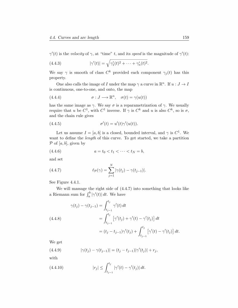
4.4. Curves and arc length 159
γ′(t) is the velocity of γ, at “time” t, and its speed is the magnitude of γ′(t):
(4.4.3) |γ′(t)| =√γ′1(t)
2 + · · ·+ γ′n(t)2.
We say γ is smooth of class Ck provided each component γj(t) has thisproperty.
One also calls the image of I under the map γ a curve in Rn. If u : J → Iis continuous, one-to-one, and onto, the map
(4.4.4) σ : J −→ Rn, σ(t) = γ(u(t))
has the same image as γ. We say σ is a reparametrization of γ. We usuallyrequire that u be C1, with C1 inverse. If γ is Ck and u is also Ck, so is σ,and the chain rule gives
(4.4.5) σ′(t) = u′(t)γ′(u(t)).
Let us assume I = [a, b] is a closed, bounded interval, and γ is C1. Wewant to define the length of this curve. To get started, we take a partitionP of [a, b], given by
(4.4.6) a = t0 < t1 < · · · < tN = b,
and set
(4.4.7) ℓP(γ) =N∑j=1
|γ(tj)− γ(tj−1)|.
See Figure 4.4.1.
We will massage the right side of (4.4.7) into something that looks like
a Riemann sum for∫ ba |γ′(t)| dt. We have
(4.4.8)
γ(tj)− γ(tj−1) =
∫ tj
tj−1
γ′(t) dt
=
∫ tj
tj−1
[γ′(tj) + γ′(t)− γ′(tj)
]dt
= (tj − tj−1)γ′(tj) +
∫ tj
tj−1
[γ′(t)− γ′(tj)
]dt.
We get
(4.4.9) |γ(tj)− γ(tj−1)| = (tj − tj−1)|γ′(tj)|+ rj ,
with
(4.4.10) |rj | ≤∫ tj
tj−1
|γ′(t)− γ′(tj)| dt.
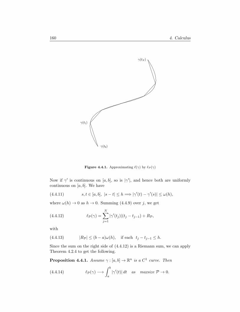
160 4. Calculus
Figure 4.4.1. Approximating ℓ(γ) by ℓP(γ)
Now if γ′ is continuous on [a, b], so is |γ′|, and hence both are uniformlycontinuous on [a, b]. We have
(4.4.11) s, t ∈ [a, b], |s− t| ≤ h =⇒ |γ′(t)− γ′(s)| ≤ ω(h),
where ω(h) → 0 as h→ 0. Summing (4.4.9) over j, we get
(4.4.12) ℓP(γ) =N∑j=1
|γ′(tj)|(tj − tj−1) +RP ,
with
(4.4.13) |RP | ≤ (b− a)ω(h), if each tj − tj−1 ≤ h.
Since the sum on the right side of (4.4.12) is a Riemann sum, we can applyTheorem 4.2.4 to get the following.
Proposition 4.4.1. Assume γ : [a, b] → Rn is a C1 curve. Then
(4.4.14) ℓP(γ) −→∫ b
a|γ′(t)| dt as maxsize P → 0.

4.4. Curves and arc length 161
We call this limit the length of the curve γ, and write
(4.4.15) ℓ(γ) =
∫ b
a|γ′(t)| dt.
Note that if u : [α, β] → [a, b] is a C1 map with C1 inverse, and σ = γu,as in (4.4.4), we have from (4.4.5) that |σ′(t)| = |u′(t)| · |γ′(u(t))|, and thechange of variable formula (4.2.67) for the integral gives
(4.4.16)
∫ β
α|σ′(t)| dt =
∫ b
a|γ′(t)| dt,
hence we have the geometrically natural result
(4.4.17) ℓ(σ) = ℓ(γ).
Given such a C1 curve γ, it is natural to consider the length function
(4.4.18) ℓγ(t) =
∫ t
a|γ′(s)| ds, ℓ′γ(t) = |γ′(t)|.
If we assume also that γ′ is nowhere vanishing on [a, b], Theorem 4.1.3, theinverse function theorem, implies that ℓγ : [a, b] → [0, ℓ(γ)] has a C1 inverse
(4.4.19) u : [0, ℓ(γ)] −→ [a, b],
and then σ = γ u : [0, ℓ(γ)] → Rn satisfies
(4.4.20)
σ′(t) = u′(t)γ′(u(t))
=1
ℓ′γ(s)γ′(u(t)), for t = ℓγ(s), s = u(t),
since the chain rule applied to u(ℓγ(t)) = t yields u′(ℓγ(t))ℓ′γ(t) = 1. Also,
by (4.18), ℓ′γ(s) = |γ′(s)| = |γ′(u(t))|, so
(4.4.21) |σ′(t)| ≡ 1.
Then σ is a reparametrization of γ, and σ has unit speed. We say σ is areparametrization by arc length.
We now focus on that most classical example of a curve in the plane R2,the unit circle
(4.4.22) S1 = (x, y) ∈ R2 : x2 + y2 = 1.
We can parametrize S1 away from (x, y) = (±1, 0) by
(4.4.23) γ+(t) = (t,√
1− t2), γ−(t) = (t,−√
1− t2),
on the intersection of S1 with (x, y) : y > 0 and (x, y) : y < 0, respec-tively. Here γ± : (−1, 1) → R2, and both maps are smooth. In fact, we can

162 4. Calculus
take γ± : [−1, 1] → R2, but these functions are not differentiable at ±1. Wecan also parametrize S1 away from (x, y) = (0,±1), by
(4.4.24) γℓ(t) = (−√
1− t2, t), γr(t) = (√
1− t2, t),
again with t ∈ (−1, 1). Note that
(4.4.25) γ′+(t) = (1,−t(1− t2)−1/2),
so
(4.4.26) |γ′+(t)|2 = 1 +t2
1− t2=
1
1− t2.
Hence, if ℓ(t) is the length of the image γ+([0, t]), we have
(4.4.27) ℓ(t) =
∫ t
0
1√1− s2
ds, for 0 < t < 1.
The same formula holds with γ+ replaced by γ−, γℓ, or γr.
We can evaluate the integral (4.4.27) as a power series in t, as follows.As seen in §3,
(4.4.28) (1− r)−1/2 =∞∑k=0
akk!rk, for |r| < 1,
where
(4.4.29) a0 = 1, a1 =1
2, ak =
(12
)(32
)· · ·
(k − 1
2
).
The power series converges uniformly on [−ρ, ρ], for each ρ ∈ (0, 1). Itfollows that
(4.4.30) (1− s2)−1/2 =
∞∑k=0
akk!s2k, |s| < 1,
uniformly convergent on [−a, a] for each a ∈ (0, 1). Hence we can integrate(4.4.30) term by term to get
(4.4.31) ℓ(t) =∞∑k=0
akk!
t2k+1
2k + 1, 0 ≤ t < 1.
One can use (4.4.27)–(4.4.31) to get a rapidly convergent infinite series forthe number π, defined as
(4.4.32) π is half the length of S1.
See Exercise 7 in §4.5.Since S1 is a smooth curve, it can be parametrized by arc length. We
will let C : R → S1 be such a parametrization, satisfying
(4.4.33) C(0) = (1, 0), C ′(0) = (0, 1),
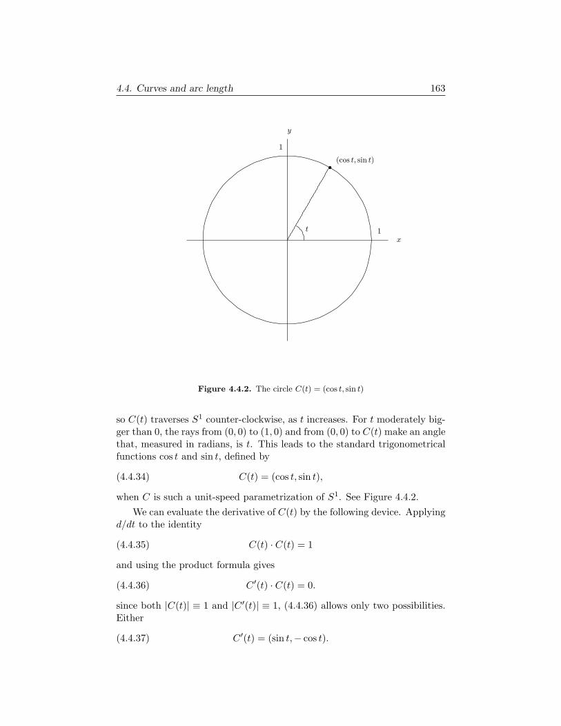
4.4. Curves and arc length 163
Figure 4.4.2. The circle C(t) = (cos t, sin t)
so C(t) traverses S1 counter-clockwise, as t increases. For t moderately big-ger than 0, the rays from (0, 0) to (1, 0) and from (0, 0) to C(t) make an anglethat, measured in radians, is t. This leads to the standard trigonometricalfunctions cos t and sin t, defined by
(4.4.34) C(t) = (cos t, sin t),
when C is such a unit-speed parametrization of S1. See Figure 4.4.2.
We can evaluate the derivative of C(t) by the following device. Applyingd/dt to the identity
(4.4.35) C(t) · C(t) = 1
and using the product formula gives
(4.4.36) C ′(t) · C(t) = 0.
since both |C(t)| ≡ 1 and |C ′(t)| ≡ 1, (4.4.36) allows only two possibilities.Either
(4.4.37) C ′(t) = (sin t,− cos t).
164 4. Calculus
or
(4.4.38) C ′(t) = (− sin t, cos t).
Since C ′(0) = (0, 1), (4.4.37) is not a possibility. This implies
(4.4.39)d
dtcos t = − sin t,
d
dtsin t = cos t.
We will derive further important results on cos t and sin t in §4.5.One can think of cos t and sin t as special functions arising to analyze
the length of arcs in the circle. Related special functions arise to analyzethe length of portions of a parabola in R2, say the graph of
(4.4.40) y =1
2x2.
This curve is parametrized by
(4.4.41) γ(t) =(t,1
2t2),
so
(4.4.42) γ′(t) = (1, t).
In such a case, the length of γ([0, t]) is
(4.4.43) ℓγ(t) =
∫ t
0
√1 + s2 ds.
Methods to evaluate the integral in (4.42) are provided in §4.5. See Exercise10 of §4.5.
The study of lengths of other curves has stimulated much work in anal-ysis. Another example is the ellipse
(4.4.44)x2
a2+y2
b2= 1,
given a, b ∈ (0,∞). This curve is parametrized by
(4.4.45) γ(t) = (a cos t, b sin t).
In such a case, by (4.38), γ′(t) = (−a sin t, b cos t), so
(4.4.46)|γ′(t)|2 = a2 sin2 t+ b2 cos2 t
= b2 + η sin2 t, η = a2 − b2,
and hence the length of γ([0, t]) is
(4.4.47) ℓγ(t) = b
∫ t
0
√1 + σ sin2 s ds, σ =
η
b2.
If a = b, this is called an elliptic integral, and it gives rise to a more subtlefamily of special functions, called elliptic functions. Material on this can befound in Chapter 6 of [14], Introduction to Complex Analysis.
4.4. Curves and arc length 165
We end this section with a brief discussion of curves in polar coordinates.We define a map
(4.4.48) Π : R2 −→ R2, Π(r, θ) = (r cos θ, r sin θ).
We say (r, θ) are polar coordinates of (x, y) ∈ R2 if Π(r, θ) = (x, y). Now, Πin (4.4.48) is not bijective, since
(4.4.49) Π(r, θ + 2π) = Π(r, θ), Π(r, θ + π) = Π(−r, θ),
and Π(0, θ) is independent of θ. So polar coordinates are not unique, butwe will not belabor this point. The point we make is that an equation
(4.4.50) r = ρ(θ), ρ : [a, b] → R,
yields a curve in R2, namely (with θ = t)
(4.4.51) γ(t) = (ρ(t) cos t, ρ(t) sin t), a ≤ t ≤ b.
The circle (4.4.34) corresponds to ρ(θ) ≡ 1. Other cases include
(4.4.52) ρ(θ) = a cos θ, −π2≤ θ ≤ π
2,
yielding a circle of diameter a/2 centered at (a/2, 0) (see Exercise 6 below),and
(4.4.53) ρ(θ) = a cos 3θ,
yielding a figure called a three-leaved rose. See Figure 4.4.3.
To compute the arc length of (4.4.51), we note that, by (4.4.39),
(4.4.54)x(t) = ρ(t) sin t, y(t) = ρ(t) sin t
⇒ x′(t) = ρ′(t) cos t− ρ(t) sin t, y′(t) = ρ′(t) sin t+ ρ(t) cos t,
hence
(4.4.55)
x′(t)2 + y′(t)2 = ρ′(t)2 cos2 t− 2ρ(t)ρ′(t) cos t sin t+ ρ(t)2 sin2 t
+ ρ′(t)2 sin2 t+ 2ρ(t)ρ′(t) sin t cos t+ ρ(t)2 cos2 t
= ρ′(t)2 + ρ(t)2.
Therefore
(4.4.56) ℓ(γ) =
∫ b
a|γ′(t)| dt =
∫ b
a
√ρ(t)2 + ρ′(t)2 dt.
Exercises
1. Let γ(t) = (t2, t3). Compute the length of γ([0, t]).
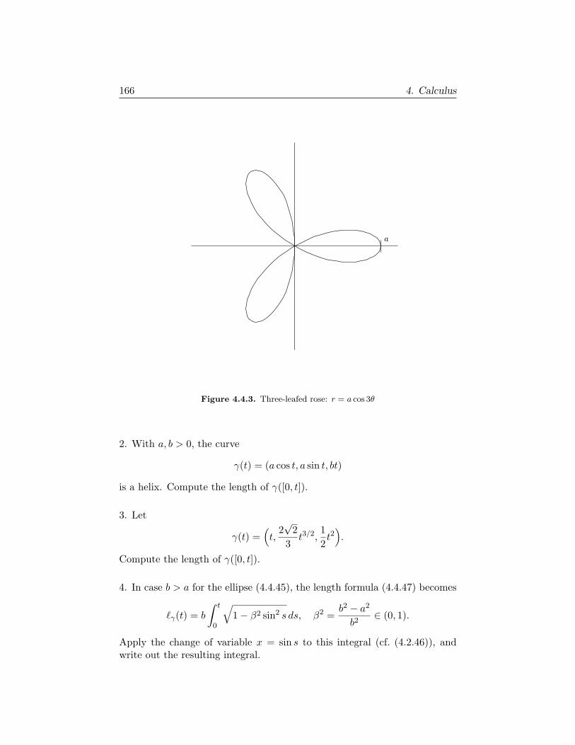
166 4. Calculus
Figure 4.4.3. Three-leafed rose: r = a cos 3θ
2. With a, b > 0, the curve
γ(t) = (a cos t, a sin t, bt)
is a helix. Compute the length of γ([0, t]).
3. Let
γ(t) =(t,2√2
3t3/2,
1
2t2).
Compute the length of γ([0, t]).
4. In case b > a for the ellipse (4.4.45), the length formula (4.4.47) becomes
ℓγ(t) = b
∫ t
0
√1− β2 sin2 s ds, β2 =
b2 − a2
b2∈ (0, 1).
Apply the change of variable x = sin s to this integral (cf. (4.2.46)), andwrite out the resulting integral.
4.4. Curves and arc length 167
5. The second half of (4.4.49) is equivalent to the identity
(cos(θ + π), sin(θ + π)) = −(cos θ, sin θ).
Deduce this from the definition (4.4.32) of π, together with the characteri-zation of C(t) in (4.4.34) as the unit speed parametrization of S1, satisfying(4.4.33). For a more general identity, see (4.5.44).
6. The curve defined by (4.4.52) can be written
γ(t) = (a cos2 t, a cos t sin t), −π2≤ t ≤ π
2.
Peek ahead at (4.5.44) and show that
γ(t) =(a2+a
2cos 2t,
a
2sin 2t
).
Verify that this traces out a circle of radius a/2, centered at (a/2, 0).
7. Use (4.4.56) to write the arc length of the curve given by (4.4.53) as anintegral. Show this integral has the same general form as (4.4.46)–(4.4.47).
8. Let γ : [a, b] → Rn be a C1 curve. Show that
ℓ(γ) ≥ |γ(b)− γ(a)|,
with strict inequality if there exists t ∈ (a, b) such that γ(t) does not lie onthe line segment from γ(a) to γ(b).Hint. To get started, show that, in (4.4.7), ℓP(γ) ≥ |γ(b)− γ(a)|.
9. Consider the curve C(t) = (cos t, sin t), discussed in (4.4.33)–(4.4.38).Note that the length ℓC(t) of C([0, t]) is t, for t > 0. Show that
C(π2
)= (0, 1), C(π) = (−1, 0), C(2π) = (1, 0).
10. In the setting of Exercise 9, compute |C(t)− (1, 0)|. Then deduce fromExercise 8 that, for 0 < t ≤ π/2,
1− cos t <t2
2,
hence (multiplying by 1 + cos t),
(4.4.57) sin2 t < t21 + cos t
2.
Hint. sin2 t = 1− cos2 t.

168 4. Calculus
11. Let γ : [a, b] → Rn be a C1 curve, and assume that |γ(t)| ≥ 1 for allt ∈ [a, b]. Set
σ(t) =1
|γ(t)|γ(t).
Show that
ℓ(σ) ≤ ℓ(γ).
Hint. Show that
x, y ∈ Rn, |x| ≥ 1, |y| ≥ 1 =⇒∣∣∣ x|x| − y
|y|
∣∣∣ ≤ |x− y|,
and deduce that ℓP(σ) ≤ ℓP(γ).
12. Consider curves γ, σ : R → R2 given by
γ(u) = (1, u), σ(u) =1
|γ(u)|γ(u),
so σ(u) lies on the unit circle centered at the origin. Show that
σ(tan t) = C(t),
where C(t) is as in (4.4.34) and
tan t =sin t
cos t.
See Figure 4.4.4.
13. With ℓγ(u) defined to be the length of γ([0, u]) and ℓσ(u) and ℓC(t)similarly defined (cf. Exercise 9), deduce from Exercises 11–12 that, for0 ≤ t < π/2,
(4.4.58) t ≤ tan t.
14. Deduce from Exercises 10 and 13 that, for 0 ≤ t < π/2,
sin t ≤ t ≤ tan t,
and hence
cos t ≤ sin t
t≤ 1.
Use this to give a demonstration that
(4.4.59) limt→0
sin t
t= 1,
independent of the use of (4.4.39).
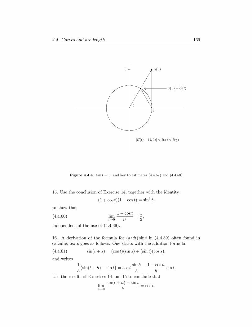
4.4. Curves and arc length 169
Figure 4.4.4. tan t = u, and key to estimates (4.4.57) and (4.4.58)
15. Use the conclusion of Exercise 14, together with the identity
(1 + cos t)(1− cos t) = sin2 t,
to show that
(4.4.60) limt→0
1− cos t
t2=
1
2,
independent of the use of (4.4.39).
16. A derivation of the formula for (d/dt) sin t in (4.4.39) often found incalculus texts goes as follows. One starts with the addition formula
(4.4.61) sin(t+ s) = (cos t)(sin s) + (sin t)(cos s),
and writes
1
h
(sin(t+ h)− sin t
)= cos t
sinh
h− 1− cosh
hsin t.
Use the results of Exercises 14 and 15 to conclude that
limh→0
sin(t+ h)− sin t
h= cos t.
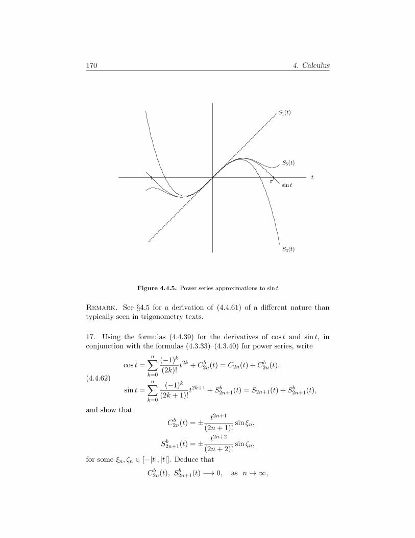
170 4. Calculus
Figure 4.4.5. Power series approximations to sin t
Remark. See §4.5 for a derivation of (4.4.61) of a different nature thantypically seen in trigonometry texts.
17. Using the formulas (4.4.39) for the derivatives of cos t and sin t, inconjunction with the formulas (4.3.33)–(4.3.40) for power series, write
(4.4.62)
cos t =n∑
k=0
(−1)k
(2k)!t2k + Cb
2n(t) = C2n(t) + Cb2n(t),
sin t =
n∑k=0
(−1)k
(2k + 1)!t2k+1 + Sb
2n+1(t) = S2n+1(t) + Sb2n+1(t),
and show that
Cb2n(t) = ± t2n+1
(2n+ 1)!sin ξn,
Sb2n+1(t) = ± t2n+2
(2n+ 2)!sin ζn,
for some ξn, ζn ∈ [−|t|, |t|]. Deduce that
Cb2n(t), S
b2n+1(t) −→ 0, as n→ ∞,
4.4. Curves and arc length 171
uniformly for t in a bounded set. See Figure 4.4.5 for graphs of sin t and thepower series approximations S1(t), S3(t), and S5(t).

172 4. Calculus
4.5. The exponential and trigonometric functions
The exponential function is one of the central objects of analysis. In thissection we define the exponential function, both for real and complex argu-ments, and establish a number of basic properties, including fundamentalconnections to the trigonometric functions.
We construct the exponential function to solve the differential equation
(4.5.1)dx
dt= x, x(0) = 1.
We seek a solution as a power series
(4.5.2) x(t) =∞∑k=0
aktk.
In such a case, if this series converges for |t| < R, then, by Proposition 4.3.2,
(4.5.3)
x′(t) =
∞∑k=1
kaktk−1
=∞∑ℓ=0
(ℓ+ 1)aℓ+1tℓ,
so for (4.5.1) to hold we need
(4.5.4) a0 = 1, ak+1 =akk + 1
,
i.e., ak = 1/k!, where k! = k(k − 1) · · · 2 · 1. Thus (4.5.1) is solved by
(4.5.5) x(t) = et =∞∑k=0
1
k!tk, t ∈ R.
This defines the exponential function et.
More generally, we can define
(4.5.6) ez =∞∑k=0
1
k!zk, z ∈ C.
The ratio test then shows that the series (4.5.6) is absolutely convergent forall z ∈ C, and uniformly convergent for |z| ≤ R, for each R <∞. Note that,again by Proposition 4.3.2,
(4.5.7) eat =∞∑k=0
ak
k!tk
solves
(4.5.8)d
dteat = aeat,
4.5. The exponential and trigonometric functions 173
and this works for each a ∈ C.We claim that eat is the unique solution to
(4.5.9)dy
dt= ay, y(0) = 1.
To see this, compute the derivative of e−aty(t):
(4.5.10)d
dt
(e−aty(t)
)= −ae−aty(t) + e−atay(t) = 0,
where we use the product rule, (4.5.8) (with a replaced by −a) and (4.5.9).Thus e−aty(t) is independent of t. Evaluating at t = 0 gives
(4.5.11) e−aty(t) = 1, ∀ t ∈ R,
whenever y(t) solves (4.5.9). Since eat solves (4.5.9), we have e−ateat = 1,hence
(4.5.12) e−at =1
eat, ∀ t ∈ R, a ∈ C.
Thus multiplying both sides of (4.5.11) by eat gives the asserted uniqueness:
(4.5.13) y(t) = eat, ∀ t ∈ R.
We can draw further useful conclusions from applying d/dt to productsof exponential functions. In fact, let a, b ∈ C; then
(4.5.14)
d
dt
(e−ate−bte(a+b)t
)= −ae−ate−bte(a+b)t − be−ate−bte(a+b)t + (a+ b)e−ate−bte(a+b)t
= 0,
so again we are differentiating a function that is independent of t. Evaluationat t = 0 gives
(4.5.15) e−ate−bte(a+b)t = 1, ∀ t ∈ R.
Again using (4.5.12), we get
(4.5.16) e(a+b)t = eatebt, ∀ t ∈ R, a, b ∈ C,
or, setting t = 1,
(4.5.17) ea+b = eaeb, ∀ a, b ∈ C.
We next record some properties of exp(t) = et for real t. The powerseries (4.5.5) clearly gives et > 0 for t ≥ 0. Since e−t = 1/et, we see thatet > 0 for all t ∈ R. Since det/dt = et > 0, the function is monotone

174 4. Calculus
increasing in t, and since d2et/dt2 = et > 0, this function is convex. (SeeProposition 4.1.5 and the remark that follows it.) Note that, for t > 0,
(4.5.18) et = 1 + t+t2
2+ · · · > 1 + t +∞,
as t ∞. Hence
(4.5.19) limt→+∞
et = +∞.
Since e−t = 1/et,
(4.5.20) limt→−∞
et = 0.
As a consequence,
(4.5.21) exp : R −→ (0,∞)
is one-to-one and onto, with positive derivative, so there is a smooth inverse
(4.5.22) L : (0,∞) −→ R.
We call this inverse the natural logarithm:
(4.5.23) log x = L(x).
See Figures 4.5.1 and 4.5.2 for graphs of x = et and t = log x.
Applying d/dt to
(4.5.24) L(et) = t
gives
(4.5.25) L′(et)et = 1, hence L′(et) =1
et,
i.e.,
(4.5.26)d
dxlog x =
1
x.
Since log 1 = 0, we get
(4.5.27) log x =
∫ x
1
dy
y.
An immediate consequence of (4.5.17) (for a, b ∈ R) is the identity
(4.5.28) log xy = log x+ log y, x, y ∈ (0,∞).
We move on to a study of ez for purely imaginary z, i.e., of
(4.5.29) γ(t) = eit, t ∈ R.
This traces out a curve in the complex plane, and we want to understandwhich curve it is. Let us set
(4.5.30) eit = c(t) + is(t),
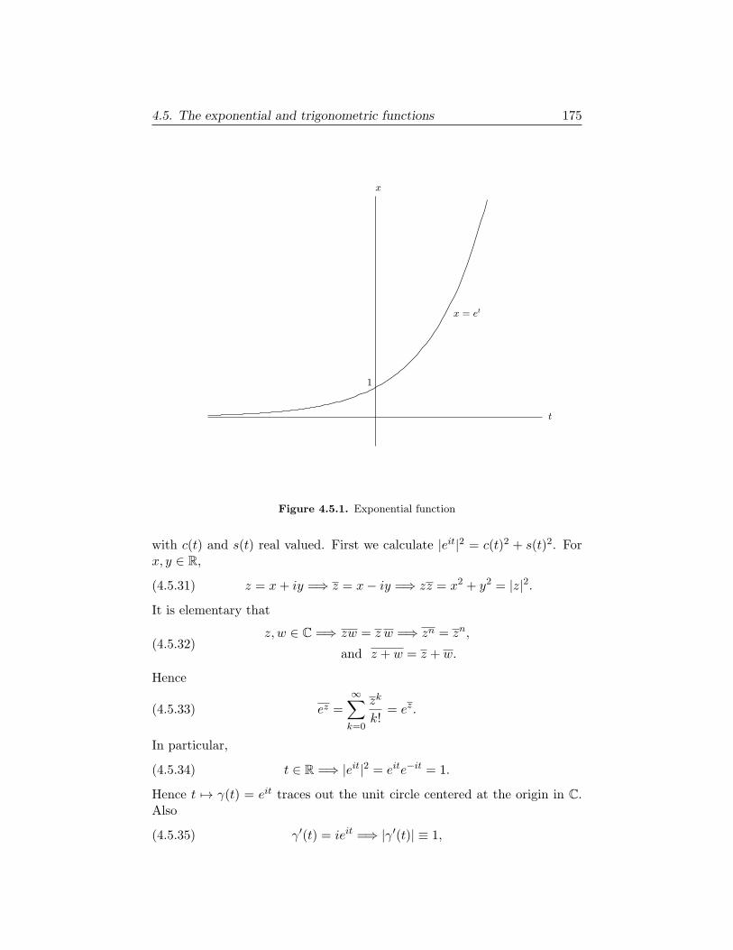
4.5. The exponential and trigonometric functions 175
Figure 4.5.1. Exponential function
with c(t) and s(t) real valued. First we calculate |eit|2 = c(t)2 + s(t)2. Forx, y ∈ R,
(4.5.31) z = x+ iy =⇒ z = x− iy =⇒ zz = x2 + y2 = |z|2.
It is elementary that
(4.5.32)z, w ∈ C =⇒ zw = z w =⇒ zn = zn,
and z + w = z + w.
Hence
(4.5.33) ez =
∞∑k=0
zk
k!= ez.
In particular,
(4.5.34) t ∈ R =⇒ |eit|2 = eite−it = 1.
Hence t 7→ γ(t) = eit traces out the unit circle centered at the origin in C.Also
(4.5.35) γ′(t) = ieit =⇒ |γ′(t)| ≡ 1,
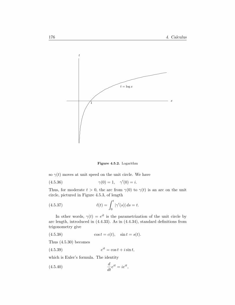
176 4. Calculus
Figure 4.5.2. Logarithm
so γ(t) moves at unit speed on the unit circle. We have
(4.5.36) γ(0) = 1, γ′(0) = i.
Thus, for moderate t > 0, the arc from γ(0) to γ(t) is an arc on the unitcircle, pictured in Figure 4.5.3, of length
(4.5.37) ℓ(t) =
∫ t
0|γ′(s)| ds = t.
In other words, γ(t) = eit is the parametrization of the unit circle byarc length, introduced in (4.4.33). As in (4.4.34), standard definitions fromtrigonometry give
(4.5.38) cos t = c(t), sin t = s(t).
Thus (4.5.30) becomes
(4.5.39) eit = cos t+ i sin t,
which is Euler’s formula. The identity
(4.5.40)d
dteit = ieit,

4.5. The exponential and trigonometric functions 177
Figure 4.5.3. The circle eit = c(t) + is(t)
applied to (4.5.39), yields
(4.5.41)d
dtcos t = − sin t,
d
dtsin t = cos t.
Compare the derivation of (4.4.39). We can use (4.5.17) to derive formulasfor sin and cos of the sum of two angles. Indeed, comparing
(4.5.42) ei(s+t) = cos(s+ t) + i sin(s+ t)
with
(4.5.43) eiseit = (cos s+ i sin s)(cos t+ i sin t)
gives
(4.5.44)cos(s+ t) = (cos s)(cos t)− (sin s)(sin t),
sin(s+ t) = (sin s)(cos t) + (cos s)(sin t).
Further material on the trigonometric functions is developed in the exercisesbelow.
Remark. An alternative approach to Euler’s formula (4.5.39) is to takethe power series for eit, via (4.5.7), and compare it to the power series for
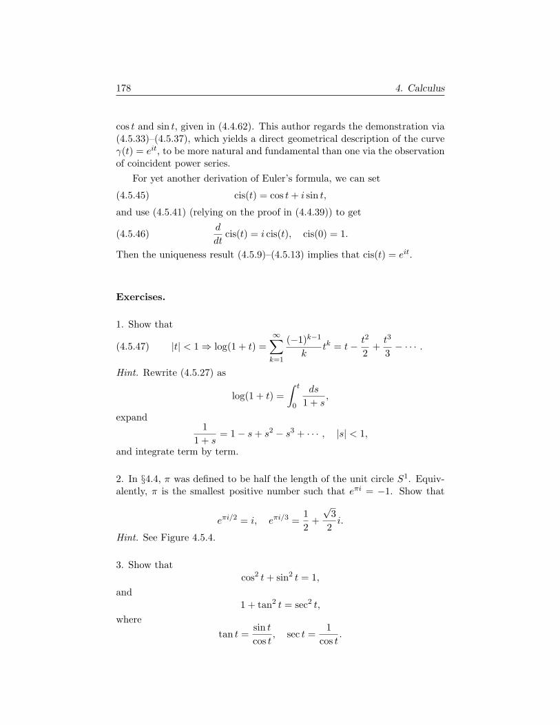
178 4. Calculus
cos t and sin t, given in (4.4.62). This author regards the demonstration via(4.5.33)–(4.5.37), which yields a direct geometrical description of the curveγ(t) = eit, to be more natural and fundamental than one via the observationof coincident power series.
For yet another derivation of Euler’s formula, we can set
(4.5.45) cis(t) = cos t+ i sin t,
and use (4.5.41) (relying on the proof in (4.4.39)) to get
(4.5.46)d
dtcis(t) = i cis(t), cis(0) = 1.
Then the uniqueness result (4.5.9)–(4.5.13) implies that cis(t) = eit.
Exercises.
1. Show that
(4.5.47) |t| < 1 ⇒ log(1 + t) =
∞∑k=1
(−1)k−1
ktk = t− t2
2+t3
3− · · · .
Hint. Rewrite (4.5.27) as
log(1 + t) =
∫ t
0
ds
1 + s,
expand1
1 + s= 1− s+ s2 − s3 + · · · , |s| < 1,
and integrate term by term.
2. In §4.4, π was defined to be half the length of the unit circle S1. Equiv-alently, π is the smallest positive number such that eπi = −1. Show that
eπi/2 = i, eπi/3 =1
2+
√3
2i.
Hint. See Figure 4.5.4.
3. Show that
cos2 t+ sin2 t = 1,
and
1 + tan2 t = sec2 t,
where
tan t =sin t
cos t, sec t =
1
cos t.
4.5. The exponential and trigonometric functions 179
Figure 4.5.4. Regular hexagon, a = eπi/3
4. Show that
d
dttan t = sec2 t = 1 + tan2 t,
d
dtsec t = sec t tan t.
5. Evaluate ∫ y
0
dx
1 + x2.
Hint. Set x = tan t.
6. Evaluate ∫ y
0
dx√1− x2
.
Hint. Set x = sin t.
180 4. Calculus
7. Show thatπ
6=
∫ 1/2
0
dx√1− x2
.
Use (4.4.27)–(4.4.31) to obtain a rapidly convergent infinite series for π.
Hint. Show that sinπ/6 = 1/2. Use Exercise 2 and the identity eπi/6 =
eπi/2e−πi/3. Note that ak in (4.4.29)-(4.4.31) satisfies ak+1 = (k + 1/2)ak.Deduce that
(4.5.48) π =
∞∑k=0
bk2k + 1
, b0 = 3, bk+1 =1
4
2k + 1
2k + 2bk.
8. Set
cosh t =1
2(et + e−t), sinh t =
1
2(et − e−t).
Show thatd
dtcosh t = sinh t,
d
dtsinh t = cosh t,
and
cosh2 t− sinh2 t = 1.
9. Evaluate ∫ y
0
dx√1 + x2
.
Hint. Set x = sinh t.
10. Evaluate ∫ y
0
√1 + x2 dx.
11. Using Exercise 4, verify that
d
dt(sec t+ tan t) = sec t(sec t+ tan t),
d
dt(sec t tan t) = sec3 t+ sec t tan2 t,
= 2 sec3 t− sec t.
12. Next verify that
d
dtlog | sec t| = tan t,
d
dtlog | sec t+ tan t| = sec t.
4.5. The exponential and trigonometric functions 181
13. Now verify that ∫tan t dt = log | sec t|,∫sec t dt = log | sec t+ tan t|,
2
∫sec3 t dt = sec t tan t+
∫sec t dt.
(Here and below, we omit the arbitrary additive constants in indefinite inte-grals.) See the next exercise, and also Exercises 40–43 for other approachesto evaluating these and related integrals.
14. Here is another approach to the evaluation of∫sec t dt. We evaluate
I(u) =
∫ u
0
dv√1 + v2
in two ways.(a) Using v = sinh y, show that
I(u) =
∫ sinh−1 u
0dy = sinh−1 u.
(b) Using v = tan t, show that
I(u) =
∫ tan−1 u
0sec t dt.
Deduce that ∫ x
0sec t dt = sinh−1(tanx), for |x| < π
2.
Deduce from this that
cosh(∫ x
0sec t dt
)= secx.
Compare these formulas with the analogue in Exercise 13. (See Exercise 45for an interesting complement.)
15. Show that
Ean(t) =
n∑k=0
ak
k!tk satisfies
d
dtEa
n(t) = aEan−1(t).
From this, show that
d
dt
(e−atEa
n(t))= −a
n+1
n!tne−at.
182 4. Calculus
16. Use Exercise 15 and the fundamental theorem of calculus to show that∫tne−at dt = − n!
an+1Ea
n(t)e−at
= − n!
an+1
(1 + at+
a2t2
2!+ · · ·+ antn
n!
)e−at.
17. Take a = −i in Exercise 16 to produce formulas for∫tn cos t dt and
∫tn sin t dt.
Exercises on xr
In §4.1, we defined xr for x > 0 and r ∈ Q. Now we define xr for x > 0 andr ∈ C, as follows:
(4.5.49) xr = er log x.
18. Show that if r = n ∈ N, (5.46) yields xn = x · · ·x (n factors).
19. Show that if r = 1/n, x1/n defined by (4.5.49) satisfies
x = x1/n · · ·x1/n (n factors),
and deduce that x1/n, defined by (4.5.49), coincides with x1/n as defined in§4.1.
20. Show that xr, defined by (4.5.49), coincides with xr as defined in §4.1,for all r ∈ Q.
21. Show that, for x > 0,
xr+s = xrxs, and (xr)s = xrs, ∀ r, s ∈ C.
22. Show that, given r ∈ C,d
dxxr = rxr−1, ∀x > 0.
22A. For y > 0, evaluate∫ y0 cos(log x) dx and
∫ x0 sin(log x) dx.
4.5. The exponential and trigonometric functions 183
Hint. Deduce from (4.5.49) and Euler’s formula that
cos(log x) + i sin(log x) = xi.
Use the result of Exercise 22 to integrate xi.
23. Show that, given r, rj ∈ C, x > 0,
rj → r =⇒ xrj → xr.
24. Given a > 0, compute
d
dxax, x ∈ R.
25. Compute
d
dxxx, x > 0.
26. Prove that
x1/x −→ 1, as x→ ∞.
Hint. Show thatlog x
x−→ 0, as x→ ∞.
27. Verify that ∫ 1
0xx dx =
∫ 1
0ex log x dx
=
∫ ∞
0e−ye−y
e−y dy
=∞∑n=1
∫ ∞
0
(−1)n
n!yne−(n+1)y dy.
28. Show that, if α > 0, n ∈ N,∫ ∞
0yne−αy dy = (−1)nF (n)(α),
where
F (α) =
∫ ∞
0e−αy dy =
1
α.
184 4. Calculus
29. Using Exercises 27–28, show that∫ 1
0xx dx =
∞∑n=0
(−1)n(n+ 1)−(n+1)
= 1− 1
22+
1
33− 1
44+ · · · .
Some special series
30. Using (4.5.47), show that
∞∑k=1
(−1)k−1
k= log 2.
Hint. Using properties of alternating series, show that if t ∈ (0, 1),
N∑k=1
(−1)k−1
ktk = log(1 + t) + rN (t), |rN (t)| ≤ tN+1
N + 1,
and let t 1.
31. Using the result of Exercise 5, show that∞∑k=0
(−1)k
2k + 1=π
4.
Hint. Exercise 5 implies
tan−1 y =
∞∑k=0
(−1)k
2k + 1y2k+1, for − 1 < y < 1.
Use an argument like that suggested for Exercise 30, taking y 1.
Alternative approach to exponentials and logs
An alternative approach is to define log : (0,∞) → R first and derive someof its properties, and then define the exponential function Exp : R → (0,∞)as its inverse. The following exercises describe how to implement this. Tostart, we take (4.5.27) as a definition:
(4.5.50) log x =
∫ x
1
dy
y, x > 0.
4.5. The exponential and trigonometric functions 185
32. Using (4.5.50), show that
(4.5.51) log(xy) = log x+ log y, ∀x, y > 0.
Also show
(4.5.52) log1
x= − log x, ∀x > 0.
33. Show from (4.5.50) that
(4.5.53)d
dxlog x =
1
x, x > 0.
34. Show that log x→ +∞ as x→ +∞.(Hint. See the hint for Exercise 15 in §4.2.)Then show that log x→ −∞ as x→ 0.
35. Deduce from Exercises 33 and 34, together with Theorem 4.1.3, that
log : (0,∞) −→ R is one-to-one and onto,
with a differentiable inverse. We denote the inverse function
Exp : R −→ (0,∞), also set et = Exp(t).
36. Deduce from Exercise 32 that
(4.5.54) es+t = eset, ∀ s, t ∈ R.
Note. (4.5.54) is a special case of (4.5.17).
37. Deduce from (4.5.53) and Theorem 4.1.3 that
(4.5.55)d
dtet = et, ∀ t ∈ R.
As a consequence,
(4.5.56)dn
dtnet = et, ∀ t ∈ R, n ∈ N.
38. Note that e0 = 1, since log 1 = 0. Deduce from (4.5.56), together withthe power series formulas (4.3.34) and (4.3.40), that, for all t ∈ R, n ∈ N,
(4.5.57) et =
n∑k=0
1
k!tk +Rn(t),
186 4. Calculus
where
(4.5.58) Rn(t) =tn+1
(n+ 1)!eζn ,
for some ζn between 0 and t.
39. Deduce from Exercise 38 that
(4.5.59) et =∞∑k=0
1
k!tk, ∀ t ∈ R.
Remark. Exercises 35–39 develop et only for t ∈ R. At this point, it is natu-ral to segue to (4.5.6) and from there to arguments involving (4.5.7)–(4.5.17),and then on to (4.5.29)–(4.5.41), renewing contact with the trigonometricfunctions.
Some more trigonometric integrals
The next few exercises treat integrals of the form
(4.5.60)
∫R(cos θ, sin θ) dθ.
Here and below, typically R is a rational function of its arguments.
40. Using the substitution x = tan θ/2, show that
dθ = 2dx
1 + x2, cos θ =
1− x2
1 + x2, sin θ =
2x
1 + x2.
Hint. With α = θ/2, use
cos 2α = 2 cos2 α− 1, and sec2 α = 1 + tan2 α.
41. Deduce that (4.5.60) converts to
(4.5.61) 2
∫R(1− x2
1 + x2,
2x
1 + x2
) dx
1 + x2.
42. Use this approach to compute∫1
sin θdθ, and
∫1
cos θdθ.
Compare the second result with that from Exercise 13.
4.5. The exponential and trigonometric functions 187
43. Use the substitution t = sin θ to show that, for k ∈ Z+,∫sec2k+1 θ dθ =
∫dt
(1− t2)k+1.
Compare what you get by the methods of Exercises 40–42, and also (fork = 0, 1) those of Exercise 13.Hint. sec2k+1 θ = (cos θ)/(1− sin2 θ)k+1.
We next look at integrals of the form
(4.5.62)
∫R(coshu, sinhu) du.
44. Using the substitution x = tanhu/2, show that
du = 2dx
1− x2, coshu =
1 + x2
1− x2, sinhu =
2x
1− x2,
and obtain an analogue of (4.5.61).
45. Looking back at Exercise 14, complement the identity
d
dtsinh−1(tan t) = sec t
withd
dutan−1(sinhu) =
1
coshu= sechu.
Compare the resulting formula for∫sechu du with what you get via Exercise
44.
We next look at integrals of the form
(4.5.63)
∫R(x,
√1 + x2) dx.
This extends results arising in Exercise 14.
46. Using the substitution x = tan θ, show that
dx = sec2 θ dθ,√
1 + x2 = sec θ,
and deduce that (4.5.63) converts to∫R( sin θ
cos θ,
1
cos θ
) 1
cos2 θdθ,
a class of integrals to which Exercises 40–41 apply.
188 4. Calculus
47. Using the substitution x = sinhu, show that
dx = coshu du,√1 + x2 = coshu,
and deduce that (4.5.63) converts to∫R(sinhu, coshu) coshu du,
a class of integrals to which Exercise 44 applies.
48. Apply the substitution x = sin θ to integrals of the form∫R(x,
√1− x2) dx,
and work out an analogue of Exercise 46.
49. We next look at arc length on the graph of t = log x. Consider the curveγ : (0,∞) → R2 given by
γ(x) = (x, log x).
Taking ℓγ(x) = ℓ(γ([1, x]) =∫ x1 |γ′(s)| ds (as in (4.4.18)), for x > 1, show
that
ℓγ(x) =
∫ x
1
√1 + y2
dy
y.
Use methods developed in Exercises 46 and/or 47 (complemented by thosedeveloped in Exercises 41 and 44) to evaluate this arc length. For anotherperspective, examine the arc length of
σ(t) = (t, et).
The gamma function
50. Show that
Γ(x) =
∫ ∞
0e−ttx−1 dt
defines
Γ : (0,∞) −→ Ras a continuous function. This is called the gamma function.
51. Show that, for x > 0,
Γ(x+ 1) = xΓ(x).
4.5. The exponential and trigonometric functions 189
Hint. Write
Γ(x+ 1) = −∫ ∞
0
( ddte−t
)tx dt,
and integrate by parts.
52. Show that Γ(1) = 1, and deduce from Exercise 51 that, for n ∈ N,
Γ(n+ 1) = n!
Remark. The gamma function has many uses in analysis. Further materialon this can be found in Chapter 3 of [13], and a good deal more can be foundin Chapter 4 of [14].
Exponentials and factorials
53. Looking at the power series for en, show that en > nn/n!, or equivalently
n! >(ne
)n.
54. We consider some more precise estimates on n!. In preparation for this,establish that, for 1 ≤ a < b <∞∫ b
alog x dx = x log x− x
∣∣∣ba.
Also, using the fact that (d2/dx2) log x < 0,
1
2
[log a+ log(a+ 1)
]<
∫ a+1
alog x dx < log(a+ 1
2).
55. Note that, for n ≥ 2,
log n! = log 2 + · · ·+ log n.
Using Exercise 54, show that∫ n
1log x dx > log 2 + · · ·+ log(n− 1) + 1
2 log n,
and hence
n! <(ne
)ne√n.
56. Similarly, using Exercise 54, show that∫ n+1/2
3/2log x dx < log 2 + · · ·+ log n,
190 4. Calculus
and hence
n! > e(n+1/2) log(n+1/2)e−(n+1/2)e−(3/2) log(3/2)e3/2.
Usinglog(n+ 1
2) = log n+ log(1 + 12n),
log(1 + δ) > δ − 12δ
2,
for 0 < δ < 1, deduce that
n! >(ne
)n[e(22
)3/2]√n.
Remark. A celebrated result known as Stirling’s formula says
(4.5.64) n! ∼(ne
)n√2πn,
as n→ ∞, in the sense that the ratio of the two sides tends to 1. We have
e(23
)3/2<
√2π < e.
Compute each of these three quantities to 5 digits of accuracy.
The gamma function is useful for proving (4.5.64). A proof can be found inAppendix A.3 of [14].
4.6. Unbounded integrable functions 191
4.6. Unbounded integrable functions
There are lots of unbounded functions we would like to be able to integrate.For example, consider f(x) = x−1/2 on (0, 1] (defined any way you like atx = 0). Since, for ε ∈ (0, 1),
(4.6.1)
∫ 1
εx−1/2 dx = 2− 2
√ε,
this has a limit as ε 0, and it is natural to set
(4.6.2)
∫ 1
0x−1/2 dx = 2.
Sometimes (4.6.2) is called an “improper integral,” but we do not considerthat to be a proper designation. Here, we define a class R#(I) of not nec-essarily bounded “integrable” functions on an interval I = [a, b], as follows.
First, assume f ≥ 0 on I, and for A ∈ (0,∞), set
(4.6.3)fA(x) = f(x) if f(x) ≤ A,
A, if f(x) > A.
We say f ∈ R#(I) provided
(4.6.4)
fA ∈ R(I), ∀A <∞, and
∃ uniform bound
∫I
fA dx ≤M.
If f ≥ 0 satisfies (4.6.4), then∫I fA dx increases monotonically to a finite
limit as A +∞, and we call the limit∫I f dx:
(4.6.5)
∫I
fA dx∫I
f dx, for f ∈ R#(I), f ≥ 0.
We also use the notation∫ ba f dx, if I = [a, b]. If I is understood, we might
just write∫f dx. It is valuable to have the following.
Proposition 4.6.1. If f, g : I → R+ are in R#(I), then f + g ∈ R#(I),and
(4.6.6)
∫I
(f + g) dx =
∫I
f dx+
∫I
g dx.
Proof. To start, note that (f + g)A ≤ fA + gA. In fact,
(4.6.7) (f + g)A = (fA + gA)A.
192 4. Calculus
Hence (f + g)A ∈ R(I) and∫(f + g)A dx ≤
∫fA dx +
∫gA dx ≤
∫f dx +∫
g dx, so we have f + g ∈ R#(I) and
(4.6.8)
∫(f + g) dx ≤
∫f dx+
∫g dx.
On the other hand, if B > 2A, then (f + g)B ≥ fA + gA, so
(4.6.9)
∫(f + g) dx ≥
∫fA dx+
∫gA dx,
for all A <∞, and hence
(4.6.10)
∫(f + g) dx ≥
∫f dx+
∫g dx.
Together, (4.6.8) and (4.6.10) yield (4.6.6).
Next, we take f : I → R and set
(4.6.11)f = f+ − f−, f+(x) = f(x) if f(x) ≥ 0,
0 if f(x) < 0.
Then we say
(4.6.12) f ∈ R#(I) ⇐⇒ f+, f− ∈ R#(I),
and set
(4.6.13)
∫I
f dx =
∫I
f+ dx−∫I
f− dx,
where the two terms on the right are defined as in (4.6.5). To extend theadditivity, we begin as follows
Proposition 4.6.2. Assume that g ∈ R#(I) and that gj ≥ 0, gj ∈ R#(I),and
(4.6.14) g = g0 − g1.
Then
(4.6.15)
∫g dx =
∫g0 dx−
∫g1 dx.
Proof. Take g = g+ − g− as in (4.6.11). Then (4.6.14) implies
(4.6.16) g+ + g1 = g0 + g−,
which by Proposition 4.6.1 yields
(4.6.17)
∫g+ dx+
∫g1 dx =
∫g0 dx+
∫g− dx.
This implies
(4.6.18)
∫g+ dx−
∫g− dx =
∫g0 dx−
∫g1 dx,

4.6. Unbounded integrable functions 193
which yields (4.6.15)
We now extend additivity.
Proposition 4.6.3. Assume f1, f2 ∈ R#(I). Then f1 + f2 ∈ R#(I) and
(4.6.19)
∫I
(f1 + f2) dx =
∫I
f1 dx+
∫I
f2 dx.
Proof. If g = f1 + f2 = (f+1 − f−1 ) + (f+2 − f−2 ), then
(4.6.20) g = g0 − g1, g0 = f+1 + f+2 , g1 = f−1 + f−2 .
We have gj ∈ R#(I), and then
(4.6.21)
∫(f1 + f2) dx =
∫g0 dx−
∫g1 dx
=
∫(f+1 + f+2 ) dx−
∫(f−1 + f−2 ) dx
=
∫f+1 dx+
∫f+2 dx−
∫f−1 dx−
∫f−2 dx,
the first equality by Proposition 4.6.2, the second tautologically, and thethird by Proposition 4.6.1. Since
(4.6.22)
∫fj dx =
∫f+j dx−
∫f−j dx,
this gives (4.6.19).
If f : I → C, we set f = f1 + if2, fj : I → R, and say f ∈ R#(I) if and
only if f1 and f2 belong to R#(I). Then we set
(4.6.23)
∫f dx =
∫f1 dx+ i
∫f2 dx.
Similar comments apply to f : I → Rn.
Given f ∈ R#(I), we set
(4.6.24) ∥f∥L1(I) =
∫I
|f(x)| dx.
We have, for f, g ∈ R#(I), a ∈ C,
(4.6.25) ∥af∥L1(I) = |a| ∥f∥L1(I),

194 4. Calculus
and
(4.6.26)
∥f + g∥L1(I) =
∫I
|f + g| dx
≤∫I
(|f |+ |g|) dx
= ∥f∥L1(I) + ∥g∥L1(I).
Note that, if S ⊂ I,
(4.6.27) cont+(S) = 0 =⇒∫I
|χS | dx = 0,
where cont+(S) is defined by (4.2.21). Thus, to get a metric, we need toform equivalence classes. The set of equivalence classes [f ] of elements ofR#(I), where
(4.6.28) f ∼ f ⇐⇒∫I
|f − f | dx = 0,
forms a metric space, with distance function
(4.6.29) D([f ], [g]) = ∥f − g∥L1(I).
However, this metric space is not complete. One needs the Lebesgue integralto obtain a complete metric space. One can see [6] or [12].
We next show that each f ∈ R#(I) can be approximated in L1 by asequence of bounded, Riemann integrable functions.
Proposition 4.6.4. If f ∈ R#(I), then there exist fk ∈ R(I) such that
(4.6.30) ∥f − fk∥L1(I) −→ 0, as k → ∞.
Proof. If we separately approximate Re f and Im f by such sequences, thenwe approximate f , so it suffices to treat the case where f is real. Similarly,writing f = f+ − f−, we see that it suffices to treat the case where f ≥ 0on I. For such f , simply take
(4.6.31) fk = fA, A = k,
with fA as in (4.6.3). Then (4.6.5) implies
(4.6.32)
∫I
fk dx∫I
f dx,

4.6. Unbounded integrable functions 195
and Proposition 4.6.3 gives
(4.6.33)
∫I
|f − fk| dx =
∫I
(f − fk) dx
=
∫I
f dx−∫I
fk dx
→ 0 as k → ∞.
So far, we have dealt with integrable functions on a bounded interval.Now, we say f : R → R (or C, or Rn) belongs to R#(R) provided f |I ∈R#(I) for each closed, bounded interval I ⊂ R and
(4.6.34) ∃A <∞ such that
∫ R
−R|f | dx ≤ A, ∀R <∞.
In such a case, we set
(4.6.35)
∫ ∞
−∞f dx = lim
R→∞
∫ R
−Rf dx.
One can similarly define R#(R+).
Exercises
1. Let f : [0, 1] → R+ and assume f is continuous on (0, 1]. Show that
f ∈ R#([0, 1]) ⇐⇒∫ 1
εf dx is bounded as ε 0.
In such a case, show that ∫ 1
0f dx = lim
ε→0
∫ 1
εf dx.
2. Let a > 0. Define pa : [0, 1] → R by pa = x−a if 0 < x ≤ 1 Set pa(0) = 0.Show that
pa ∈ R#([0, 1]) ⇐⇒ a < 1.
3. Let b > 0. Define qb : [0, 1/2] → R by
qb(x) =1
x| log x|b,

196 4. Calculus
if 0 < x ≤ 1/2. Set qb(0) = 0. Show that
qb ∈ R#([0, 1/2]) ⇐⇒ b > 1.
4. Show that if a ∈ C and if f ∈ R#(I), then
af ∈ R#(I), and
∫af dx = a
∫f dx.
Hint. Check this for a > 0, a = −1, and a = i.
5. Show that
f ∈ R(I), g ∈ R#(I) =⇒ fg ∈ R#(I).
Hint. Use (4.2.53). First treat the case f, g ≥ 1, f ≤M . Show that in sucha case,
(fg)A = (fAgA)A, and (fg)A ≤MgA.
6. Compute ∫ 1
0log t dt.
Hint. To compute∫ 1ε log t dt, first compute
d
dt(t log t).
7. Given g ∈ R(I), show that there exist gk ∈ PK(I) such that
∥g − gk∥L1(I) −→ 0.
Given h ∈ PK(I), show that there exist hk ∈ C(I) such that
∥h− hk∥L1(I) −→ 0.
8. Using Exercise 7 and Proposition 4.6.4, prove the following: given f ∈R#(I), there exist fk ∈ C(I) such that
∥f − fk∥L1(I) −→ 0.
9. Recall Exercise 4 of §4.2. If φ : [a, b] → [A,B] is C1, with φ′(x) > 0 forall x ∈ [a, b], then
(4.6.36)
∫ B
Af(y) dy =
∫ b
af(φ(t))φ′(t) dt,
for each f ∈ C([a, b]), where A = φ(a), B = φ(b). Using Exercise 8, showthat (4.6.36) holds for each f ∈ R#([a, b]).
4.6. Unbounded integrable functions 197
10. If f ∈ R#(R), so (4.6.34) holds, prove that the limit exists in (4.6.35).
11. Given f(x) = x−1/2(1 + x2)−1 for x > 0, show that f ∈ R#(R+). Showthat ∫ ∞
0
1
1 + x2dx√x= 2
∫ ∞
0
dy
1 + y4.
12. Let fk ∈ R#([a, b]), f : [a, b] → R satisfy
(a) |fk| ≤ g, ∀ k, for some g ∈ R#([a, b]),
(b) Given ε > 0, ∃ contented Sε ⊂ [a, b] such that∫Sε
g dx < ε, and fk → f uniformly on [a, b] \ Sε.
Show that f ∈ R#([a, b]) and∫ b
afk(x) dx −→
∫ b
af(x) dx, as k → ∞.
13. Let g ∈ R#([a, b]) be ≥ 0. Show that for each ε > 0, there exists δ > 0such that
S ⊂ [a, b] contented, contS < δ =⇒∫S
g dx < ε.
Hint. With gA defined as in (4.6.3), pick A such that∫gA dx ≥
∫g dx−ε/2.
Then pick δ < ε/2A.
14. Deduce from Exercises 12–13 the following. Let fk ∈ R#([a, b]), f :[a, b] → R satisfy
(a) |fk| ≤ g, ∀ k, for some g ∈ R#([a, b]),
(b) Given δ > 0, ∃ contented Sδ ⊂ [a, b] such that
contSδ < δ, and fk → f uniformly on [a, b] \ Sδ.
Show that f ∈ R#([a, b]) and∫ b
afk(x) dx −→
∫ b
af(x) dx, as k → ∞.
Remark. Compare Exercise 18 of §4.2. As mentioned there, the Lebesguetheory of integration has a stronger result, known as the Lebesgue dominatedconvergence theorem.

198 4. Calculus
15. Given g(s) = 1/√1− s2, show that g ∈ R#([−1, 1]), and that∫ 1
−1
ds√1− s2
= π.
Compare the arc length formula (4.4.27).
16. Given f(t) = 1/√t(1− t), show that f ∈ R#([0, 1]), and that∫ 1
0
dt√t(1− t)
= π.
Hint. Set t = s2.
Chapter 5
Further Topics inAnalysis
In this final chapter we apply results of Chapters 3 and 4 to a selection oftopics in analysis. One underlying theme here is the approximation of afunction by a sequence of “simpler” functions.
In §5.1 we define the convolution of functions on R,
f ∗ u(x) =∫ ∞
−∞f(y)u(x− y) dy,
and give conditions on a sequence (fn) guaranteeing that fn ∗ u → u asn → ∞. In §5.2 we treat the Weierstrass approximation theorem, whichstates that each continuous function on a closed, bounded interval [a, b] is auniform limit of a sequence of polynomials. We give two proofs, one usingconvolutions and one using the uniform convergence on [−1, 1] of the powerseries of (1 − x)b, whenever b > 0, which we establish in Appendix A.2.(Here, we take b = 1/2.) Section 5.3 treats a far reaching generalization,known as the Stone-Weierstrass theorem. A special case, of use in §5.4, isthat each continuous function on T1 is a uniform limit of a sequence of finitelinear combinations of the exponentials eikθ, k ∈ Z.
Section 5.4 introduces Fourier series,
f(θ) =∞∑
k=−∞ake
ikθ.
A central question is when this holds with
ak =1
2π
∫ π
−πf(θ)e−ikθ dθ.
199
200 5. Further Topics in Analysis
This is the Fourier inversion problem, and we examine several aspects ofthis. Fourier analysis is a major area in modern analysis. Material treatedhere will provide a useful background (and stimulus) for further study.
We mention that Chapter 3 of [14] deals with Fourier series on a similarlevel as here, while making contact with complex analysis, and also includingtreatments of the Fourier transform and Laplace transform. Progressivelymore advanced treatments of Fourier analysis can be found in [13], Chapter7, [6], Chapter 8, and [15], Chapter 3.
Section 5.5 treats the use of Newton’s method to solve
f(ξ) = y
for ξ in an interval [a, b] given that f(a)−y and f(b)−y have opposite signsand that
|f ′′(x)| ≤ A, |f ′(x)| ≥ B > 0, ∀x ∈ [a, b].
It is seen that if an initial guess x0 is close enough to ξ, then Newton’smethod produces a sequence (xk) satisfying
|xk − ξ| ≤ Cβ2k, for some β ∈ (0, 1).
It is extremely useful to have such a rapid approximation of the solution ξ.
This chapter also has an appendix, §5.6, dealing with inner productspaces. This class of space generalizes the notion of Euclidean spaces, con-sidered in §2.1, from finite to infinite dimensions. The results are of use inour treatment of Fourier series, in §5.4.
5.1. Convolutions and bump functions
If u is bounded and continuous on R and f is integrable (say f ∈ R(R)) wedefine the convolution f ∗ u by
(5.1.1) f ∗ u(x) =∫ ∞
−∞f(y)u(x− y) dy.
Clearly
(5.1.2)
∫|f | dx = A, |u| ≤M on R =⇒ |f ∗ u| ≤ AM on R.
Also, a change of variable gives
(5.1.3) f ∗ u(x) =∫ ∞
−∞f(x− y)u(y) dy.
We want to analyze the convolution action of a sequence of integrablefunctions fn on R that satisfy the following conditions:
(5.1.4) fn ≥ 0,
∫fn dx = 1,
∫R\In
fn dx = εn → 0,
5.1. Convolutions and bump functions 201
where
(5.1.5) In = [−δn, δn], δn → 0.
Let u ∈ C(R) be supported on a bounded interval [−A,A], or more generally,assume
(5.1.6) u ∈ C(R), |u| ≤M on R,
and u is uniformly continuous on R, so with δn as in (5.1.5),
(5.1.7) |x− x′| ≤ 2δn =⇒ |u(x)− u(x′)| ≤ εn → 0.
We aim to prove the following.
Proposition 5.1.1. If fn ∈ R(R) satisfy (5.1.4)–(5.1.5) and if u ∈ C(R) isbounded and uniformly continuous (satisfying (5.1.6)–(5.1.7)), then
(5.1.8) un = fn ∗ u −→ u, uniformly on R, as n→ ∞.
Proof. To start, write
(5.1.9)
un(x) =
∫fn(y)u(x− y) dy
=
∫In
fn(y)u(x− y) dy +
∫R\In
fn(y)u(x− y) dy
= vn(x) + rn(x).
Clearly
(5.1.10) |rn(x)| ≤Mεn, ∀x ∈ R.
Next,
(5.1.11) vn(x)− u(x) =
∫In
fn(y)[u(x− y)− u(x)] dy − εnu(x),
so
(5.1.12) |vn(x)− u(x)| ≤ εn +Mεn, ∀x ∈ R,
hence
(5.1.13) |un(x)− u(x)| ≤ εn + 2Mεn, ∀x ∈ R,
yielding (5.1.8).
Here is a sequence of functions (fn) satisfying (5.1.4)–(5.1.5). First, set
(5.1.14) gn(x) =1
An(x2 − 1)n, An =
∫ 1
−1(x2 − 1)n dx,
202 5. Further Topics in Analysis
and then set
(5.1.15)fn(x) = gn(x), |x| ≤ 1,
0, |x| ≥ 1.
It is readily verified that such (fn) satisfy (5.1.4)–(5.1.5). We will use thissequence in Proposition 5.1.1 for one proof of the Weierstrass approximationtheorem, in the next section.
The functions fn defined by (5.1.14)–(5.1.15) have the property
(5.1.16) fn ∈ Cn−1(R).
Furthermore, they have compact support, i.e., vanish outside some compactset. We say
(5.1.17) f ∈ Ck0 (R),
provided f ∈ Ck(R) and f has compact support. The following result isuseful.
Proposition 5.1.2. If f ∈ Ck0 (R) and u ∈ R(R), then f ∗ u ∈ Ck(R), and
(provided k ≥ 1)
(5.1.18)d
dxf ∗ u(x) = f ′ ∗ u(x).
Proof. We start with the case k = 0, and show that
f ∈ C00 (R), u ∈ R(R) =⇒ f ∗ u ∈ C(R).
In fact, by (5.1.3),∣∣∣f ∗ u(x+ h)− f ∗ u(x)∣∣∣ = ∣∣∣∫ ∞
−∞[f(x+ h− y)− f(x− y)]u(y) dy
∣∣∣≤ sup
x|f(x+ h)− f(x)|
∫ ∞
−∞|u(y)| dy,
which clearly tends to 0 as h→ 0.
From here, it suffices to treat the case k = 1, since if f ∈ Ck0 (R), then
f ′ ∈ Ck−10 (R), and one can use induction on k. Using (5.1.3), we have
(5.1.19)f ∗ u(x+ h)− f ∗ u(x)
h=
∫ ∞
−∞gh(x− y)u(y) dy,
where
(5.1.20) gh(x) =1
h[f(x+ h)− f(x)].
We claim that
(5.1.21) f ∈ C10 (R) =⇒ gh → f ′ uniformly on R, as h→ 0.
5.1. Convolutions and bump functions 203
Given this,
(5.1.22)
∣∣∣∫ ∞
−∞gh(x− y)u(y) dy −
∫ ∞
−∞f ′(x− y)u(y) dy
∣∣∣≤ sup
x|gh(x)− f ′(x)|
∫ ∞
−∞|u(y)| dy,
which yields (5.1.18).
It remains to prove (5.1.21). Indeed, the fundamental theorem of calcu-lus implies
(5.1.23) gh(x) =1
h
∫ x+h
xf ′(y) dy,
if h > 0, so
(5.1.24) |gh(x)− f ′(x)| ≤ supx≤y≤x+h
|f ′(y)− f ′(x)|,
if h > 0, with a similar estimate if h < 0. This yields (5.1.21).
We say
(5.1.25) f ∈ C∞(R) provided f ∈ Ck(R) for all k,
and similarly f ∈ C∞0 (R) provided f ∈ Ck
0 (R), for all k. It is useful to havesome examples of functions in C∞
0 (R). We start with the following. Set
(5.1.26)G(x) = e−1/x2
, if x > 0,
0, if x ≤ 0.
Lemma 5.1.3. G ∈ C∞(R).
Proof. Clearly g ∈ Ck for all k on (0,∞) and on (−∞, 0). We need tocheck its behavior at 0. The fact that G is continuous at 0 follows from
(5.1.27) e−y2 −→ 0, as y → ∞.
Note that
(5.1.28)G′(x) =
2
x3e−1/x2
, if x > 0,
0, if x < 0.
also
(5.1.29) G′(0) = limh→0
G(h)
h= 0,
as a consequence of
(5.1.30) ye−y2 −→ 0, as y → ∞.
204 5. Further Topics in Analysis
Clearly G′ is continuous on (0,∞) and on (−∞, 0). The continuity at 0 is aconsequence of
(5.1.31) y3e−y2 −→ 0, as y → ∞.
The existence and continuity of higher derivatives of G follows a similarpattern, making use of
(5.1.32) yke−y2 −→ 0, as y → ∞,
for each k ∈ N. We leave the details to the reader.
Corollary 5.1.4. Set
(5.1.33) g(x) = G(x)G(1− x).
Then g ∈ C∞0 (R). In fact, g(x) = 0 if and only if 0 < x < 1.
Exercises
1. Let f ∈ R(R) satisfy
(5.1.34) f ≥ 0,
∫f dx = 1,
and set
(5.1.35) fn(x) = nf(xn
), n ∈ N.
Show that Proposition 5.1.1 applies to the sequence fn.
2. Take
(5.1.36) f(x) =1
Ae−x2
, A =
∫ ∞
−∞e−x2
dx.
Show that Exercise 1 applies to this case.Note. In [13] it is shown that A =
√π in (5.1.36).
3. Modify the proof of Lemma 5.1.3 to show that, if
G1(x) = e−1/x, if x > 0,
0, if x ≤ 0,
then G1 ∈ C∞(R).
4. Establish whether each of the following functions is in C∞(R).
φ(x) = G(x) sin1
x, if x = 0,
0, if x = 0.
5.2. The Weierstrass approximation theorem 205
ψ(x) = G1(x) sin1
x, if x = 0,
0, if x = 0.
Here G(x) is as in (5.1.26) and G1(x) is as in Exercise 3.
5.2. The Weierstrass approximation theorem
The following result of Weierstrass is a very useful tool in analysis.
Theorem 5.2.1. Given a compact interval I, any continuous function f onI is a uniform limit of polynomials.
Otherwise stated, our goal is to prove that the space C(I) of continuous(real valued) functions on I is equal to P(I), the uniform closure in C(I) ofthe space of polynomials.
We will give two proofs of this theorem. Our starting point for the firstproof will be the result that the power series for (1−x)a converges uniformlyon [−1, 1], for any a > 0. This is established in Appendix A.2, and we willuse it, with a = 1/2.
From the identity x1/2 = (1− (1−x))1/2, we have x1/2 ∈ P([0, 2]). Moreto the point, from the identity
(5.2.1) |x| =(1− (1− x2)
)1/2,
we have |x| ∈ P([−√2,√2]). Using |x| = b−1|bx|, for any b > 0, we see that
|x| ∈ P(I) for any interval I = [−c, c], and also for any closed subinterval,hence for any compact interval I. By translation, we have
(5.2.2) |x− a| ∈ P(I)
for any compact interval I. Using the identities
(5.2.3) max(x, y) =1
2(x+ y)+
1
2|x− y|, min(x, y) =
1
2(x+ y)− 1
2|x− y|,
we see that for any a ∈ R and any compact I,
(5.2.4) max(x, a), min(x, a) ∈ P(I).
We next note that P(I) is an algebra of functions, i.e.,
(5.2.5) f, g ∈ P(I), c ∈ R =⇒ f + g, fg, cf ∈ P(I).
Using this, one sees that, given f ∈ P(I), with range in a compact intervalJ , one has h f ∈ P(I) for all h ∈ P(J). Hence f ∈ P(I) ⇒ |f | ∈ P(I),and, via (5.2.3), we deduce that
(5.2.6) f, g ∈ P(I) =⇒ max(f, g), min(f, g) ∈ P(I).

206 5. Further Topics in Analysis
Suppose now that I ′ = [a′, b′] is a subinterval of I = [a, b]. With thenotation x+ = max(x, 0), we have
(5.2.7) fII′(x) = min((x− a′)+, (b
′ − x)+)∈ P(I).
This is a piecewise linear function, equal to zero off I \ I ′, with slope 1 froma′ to the midpoint m′ of I ′, and slope −1 from m′ to b′.
Now if I is divided into N equal subintervals, any continuous functionon I that is linear on each such subinterval can be written as a linear combi-nation of such “tent functions,” so it belongs to P(I). Finally, any f ∈ C(I)can be uniformly approximated by such piecewise linear functions, so wehave f ∈ P(I), proving the theorem.
For the second proof, we bring in the sequence of functions fn definedby (5.1.14)–(5.1.15), i.e., first set
(5.2.8) gn(x) =1
An(x2 − 1)n, An =
∫ 1
−1(x2 − 1)n dx,
and then set
(5.2.9)fn(x) = gn(x), |x| ≤ 1,
0, |x| ≥ 1.
It is readily verified that such (fn) satisfy (5.1.4)–(5.1.5). We will use thissequence in Proposition 5.1.1 to prove that if I ⊂ R is a closed, boundedinterval, and f ∈ C(I), then there exist polynomials pn(x) such that
(5.2.10) pn −→ f, uniformly on I.
To start, we note that by an affine change of variable, there is no loss ofgenerality in assuming that
(5.2.11) I =[−1
4,1
4
].
Next, given I as in (5.2.11) and f ∈ C(I), it is easy to extend f to a function
(5.2.12) u ∈ C(R), u(x) = 0 for |x| ≥ 1
2.
Now, with fn as in (5.2.8)–(5.2.9), we can apply Proposition 5.1.1 to deducethat
(5.2.13) un(x) =
∫fn(y)u(x− y) dy =⇒ un → u uniformly on R.
Now
(5.2.14)|x| ≤ 1
2=⇒ u(x− y) = 0 for |y| > 1
=⇒ un(x) =
∫gn(y)u(x− y) dy,

5.2. The Weierstrass approximation theorem 207
that is,
(5.2.15) |x| ≤ 1
2=⇒ un(x) = pn(x),
where
(5.2.16)
pn(x) =
∫gn(y)u(x− y) dy
=
∫gn(x− y)u(y) dy.
The last identity makes it clear that each pn(x) is a polynomial in x. Since(5.2.13) and (5.2.15) imply
(5.2.17) pn −→ u uniformly on[−1
2,1
2
],
we have (5.2.10).
Exercises
1. As in Exercises 1–2 of §5.1, take
f(x) =1
Ae−x2
, A =
∫ ∞
−∞e−x2
dx,
fn(x) = nf(xn
).
Let u ∈ C(R) vanish outside [−1, 1]. Let ε > 0 and take n ∈ N such that
supx
|fn ∗ u(x)− u(x)| < ε.
Approximate fn by a sufficient partial sum of the power series
fn(x) =n
A
∞∑k=0
1
k!
(−x
2
n2
)k,
and use this to obtain a third proof of Theorem 5.2.1.
Remark. A fourth proof of Theorem 5.2.1 is indicated in Exercise 8 of §5.4.
2. Let f be continuous on [−1, 1]. If f is odd, show that it is a uniform limitof finite linear combinations of x, x3, x5, . . . , x2k+1, . . . . If f is even, show itis a uniform limit of finite linear combinations of 1, x2, x4, . . . , x2k, . . . .
3. If g is continuous on [−π/2, π/2], show that g is a uniform limit of finitelinear combinations of
sinx, sin2 x, sin3 x, . . . , sink x, . . . .
208 5. Further Topics in Analysis
Hint. Write g(x) = f(sinx) with f continuous on [−1, 1].
4. If g is continuous on [−π, π] and even, show that g is a uniform limit offinite linear combinations of
1, cosx, cos2 x, . . . , cosk x, . . . .
Hint. cos : [0, π] → [−1, 1] is a homeomorphism.
5. Assume h : R → C is continuous, periodic of period 2π, and odd, so
(5.2.18) h(x+ 2π) = h(x), h(−x) = −h(x), ∀x ∈ R.Show that h is a uniform limit of finite linear combinations of
sinx, sinx cosx, sinx cos2 x, . . . , sinx cosk x, . . . .
Hint. Given ε > 0, find δ > 0 and continuous hε, satisfying (5.2.18), suchthat
supx
|h(x)− hε(x)| < ε, hε(x) = 0 if |x− jπ| < δ, j ∈ Z.
Then apply Exercise 4 to g(x) = hε(x)/ sinx.
5.3. The Stone-Weierstrass theorem
A far reaching extension of the Weierstrass approximation theorem, due toM. Stone, is the following result, known as the Stone-Weierstrass theorem.
Theorem 5.3.1. Let X be a compact metric space, A a subalgebra ofCR(X), the algebra of real valued continuous functions on X. Suppose 1 ∈ Aand that A separates points of X, i.e., for distinct p, q ∈ X, there existshpq ∈ A with hpq(p) = hpq(q). Then the closure A is equal to CR(X).
We will derive this from the following lemma.
Lemma 5.3.2. Let A ⊂ CR(X) satisfy the hypotheses of Theorem 5.3.1,and let K, L ⊂ X be disjoint, compact subsets of X. Then there existsgKL ∈ A such that
(5.3.1) gKL = 1 on K, 0 on L, and 0 ≤ gKL ≤ 1 on X.
Proof of Theorem 5.3.1 To start, take f ∈ CR(X) such that 0 ≤ f ≤ 1on X. Set
(5.3.2) K = x ∈ X : f(x) ≥ 23, U = x ∈ X : f(x) > 1
3, L = X \ U.
Lemma 5.3.2 implies that there exists g ∈ A such that
(5.3.3) g =1
3on K, g = 0 on L, and 0 ≤ g ≤ 1
3.
5.3. The Stone-Weierstrass theorem 209
Then 0 ≤ g ≤ f ≤ 1 on X, and more precisely
(5.3.4) 0 ≤ f − g ≤ 2
3, on X.
We can apply such reasoning with f replaced by f − g, obtaining g2 ∈ Asuch that
(5.3.5) 0 ≤ f − g − g2 ≤(23
)2, on X,
and iterate, obtaining gj ∈ A such that, for each k,
(5.3.6) 0 ≤ f − g − g2 − · · · − gk ≤(23
)k, on X.
This yields f ∈ A whenever f ∈ CR(X) satisfies 0 ≤ f ≤ 1. It is an easystep to see that f ∈ CR(X) ⇒ f ∈ A.
Proof of Lemma 5.3.2. We present the proof in six steps.
Step 1. Let f ∈ A and assume φ : R → R is continuous. If sup |f | ≤ A,we can apply the Weierstrass approximation theorem to get polynomialspk → φ uniformly on [−A,A]. Then pk f → φ f uniformly on X, soφ f ∈ A.
Step 2. Consequently, if fj ∈ A, then
(5.3.7) max(f1, f2) =1
2|f1 − f2|+
1
2(f1 + f2) ∈ A,
and similarly min(f1, f2) ∈ A.
Step 3. It follows from the hypotheses that if p, q ∈ X and p = q, thenthere exists fpq ∈ A, equal to 1 at p and to 0 at q.
Step 4. Apply an appropriate continuous φ : R → R to get gpq = φ fpq ∈A, equal to 1 on a neighborhood of p and to 0 on a neighborhood of q, andsatisfying 0 ≤ gpq ≤ 1 on X.
Step 5. Let L ⊂ X be compact and fix p ∈ X \ L. By Step 4, given q ∈ L,there exists gpq ∈ A such that gpq = 1 on a neighborhood Oq of p, equal to0 on a neighborhood Ωq of q, satisfying 0 ≤ gpq ≤ 1 on X.

210 5. Further Topics in Analysis
Now Ωq is an open cover of L, so there exists a finite subcover Ωq1 , . . . ,ΩqN .Let
(5.3.8) gpL = min1≤j≤N
gpqj ∈ A.
Taking O = ∩N1 Oqj , an open neighborhood of p, we have
(5.3.9) gpL = 1 on O, 0 on L, and 0 ≤ gpL ≤ 1 on X.
Step 6. Take K, L ⊂ X disjoint, compact subsets. By Step 5, for eachp ∈ K, there exists gpL ∈ A, equal to 1 on a neighborhood Op of p, andequal to 0 on L.
Now Op covers K, so there exists a finite subcover Op1 , . . . ,OpM . Let
(5.3.10) gKL = max1≤j≤M
gpjL ∈ A.
We have
(5.3.11) gKL = 1 on K, 0 on L, and 0 ≤ gKL ≤ 1 on X,
as asserted in the lemma.
Theorem 5.3.1 has a complex analogue.
Theorem 5.3.3. Let X be a compact metric space, A a subalgebra (over C)of C(X), the algebra of complex valued continuous functions on X. Suppose1 ∈ A and that A separates the points of X. Furthermore, assume
(5.3.12) f ∈ A =⇒ f ∈ A.
Then the closure A = C(X).
Proof. Set AR = f + f : f ∈ A. One sees that Theorem 5.3.1 applies toAR.
Here are a couple of applications of Theorems 5.3.1–5.3.3.
Corollary 5.3.4. If X is a compact subset of Rn, then every f ∈ C(X) isa uniform limit of polynomials on Rn.
Corollary 5.3.5. The space of trigonometric polynomials, given by
(5.3.13)
N∑k=−N
ak eikθ,
is dense in C(S1).
5.3. The Stone-Weierstrass theorem 211
Exercises
1. Prove Corollary 5.3.4.
2. Prove Corollary 5.3.5, using Theorem 5.3.3.
Hint. eikθeiℓθ = ei(k+ℓ)θ, and eikθ = e−ikθ.
3. Use the results of Exercises 4–5 in §5.2 to provide another proof ofCorollary 5.3.5.Hint. Use cosk θ = ((eiθ + e−iθ)/2)k, etc.
4. Let X be a compact metric space, and K ⊂ X a compact subset. Showthat A = f |K : f ∈ C(X) is dense in C(K).
5. In the setting of Exercise 4, take f ∈ C(K), ε > 0. Show that thereexists g1 ∈ C(X) such that
supK
|g1 − f | ≤ ε, and supX
|g1| ≤ supK
|f |.
6. Iterate the result of Exercise 5 to get gk ∈ C(X) such that
supK
|gk − (f − g1 − · · · − gk−1)| ≤ 2−k, supX
|gk| ≤ 2−(k−1).
7. Use the results of Exercises 4–6 to show that, if f ∈ C(K), then thereexists g ∈ C(X) such that g|K = f .

212 5. Further Topics in Analysis
5.4. Fourier series
We work on T1 = R/(2πZ), which under θ 7→ eiθ is equivalent to S1 = z ∈C : |z| = 1. Given f ∈ C(T1), or more generally f ∈ R(T1) (or still moregenerally, if f ∈ R#(T1), defined as in §4.6 of Chapter 4), we set, for k ∈ Z,
(5.4.1) f(k) =1
2π
∫ 2π
0f(θ)e−ikθ dθ.
We call f(k) the Fourier coefficients of f . We say
(5.4.2) f ∈ A(T1) ⇐⇒∞∑
k=−∞|f(k)| <∞.
Our first goal is to prove the following.
Proposition 5.4.1. Given f ∈ C(T1), if f ∈ A(T1), then
(5.4.3) f(θ) =
∞∑k=−∞
f(k)eikθ.
Proof. Given∑
|f(k)| < ∞, the right side of (5.4.3) is absolutely anduniformly convergent, defining
(5.4.4) g(θ) =
∞∑k=−∞
f(k)eikθ, g ∈ C(T1),
and our task is to show that f ≡ g. Making use of the identities
(5.4.5)
1
2π
∫ 2π
0eiℓθ dθ = 0, if ℓ = 0,
1, if ℓ = 0,
we get f(k) = g(k), for all k ∈ Z. Let us set u = f − g. We have
(5.4.6) u ∈ C(T1), u(k) = 0, ∀ k ∈ Z.It remains to show that this implies u ≡ 0. To prove this, we use Corollary5.3.5, which implies that, for each v ∈ C(T1), there exist trigonometricpolynomials, i.e., finite linear combinations vN of eikθ : k ∈ Z, such that
(5.4.7) vN −→ v uniformly on T1.
Now (5.4.6) implies ∫T1
u(θ)vN (θ) dθ = 0, ∀N,
and passing to the limit, using (5.4.7), gives
(5.4.8)
∫T1
u(θ)v(θ) dθ = 0, ∀ v ∈ C(T1).
5.4. Fourier series 213
Taking v = u gives
(5.4.9)
∫T1
|u(θ)|2 dθ = 0,
forcing u ≡ 0, and completing the proof.
We seek conditions on f that imply (5.4.2). Integration by parts forf ∈ C1(T1) gives, for k = 0,
(5.4.10)
f(k) =1
2π
∫ 2π
0f(θ)
i
k
∂
∂θ(e−ikθ) dθ
=1
2πik
∫ 2π
0f ′(θ)e−ikθ dθ,
hence
(5.4.11) |f(k)| ≤ 1
2π|k|
∫ 2π
0|f ′(θ)| dθ.
If f ∈ C2(T1), we can integrate by parts a second time, and get
(5.4.12) f(k) = − 1
2πk2
∫ 2π
0f ′′(θ)e−ikθ dθ,
hence
|f(k)| ≤ 1
2πk2
∫ 2π
0|f ′′(θ)| dθ.
In concert with
(5.4.13) |f(k)| ≤ 1
2π
∫ 2π
0|f(θ)| dθ,
which follows from (5.4.1), we have
(5.4.14) |f(k)| ≤ 1
2π(k2 + 1)
∫ 2π
0
[|f ′′(θ)|+ |f(θ)|
]dθ.
Hence
(5.4.15) f ∈ C2(T1) =⇒∑
|f(k)| <∞.
We will sharpen this implication below. We start with an interestingexample. Consider
(5.4.16) f(θ) = |θ|, −π ≤ θ ≤ π,
and extend this to be periodic of period 2π, yielding f ∈ C(T1). We have
(5.4.17)
f(k) =1
2π
∫ π
−π|θ|e−ikθ dθ =
1
π
∫ π
0θ cos kθ dθ
= −[1− (−1)k]1
πk2,

214 5. Further Topics in Analysis
for k = 0, while f(0) = π/2. This is clearly a summable series, so f ∈ A(T1),and Proposition 5.4.1 implies that, for −π ≤ θ ≤ π,
(5.4.18)
|θ| = π
2−
∑k odd
2
πk2eikθ
=π
2− 4
π
∞∑ℓ=0
1
(2ℓ+ 1)2cos(2ℓ+ 1)θ.
Now, evaluating this at θ = 0 yields the identity
(5.4.19)
∞∑ℓ=0
1
(2ℓ+ 1)2=π2
8.
Using this, we can evaluate
(5.4.20) S =
∞∑k=1
1
k2,
as follows. We have
(5.4.21)
∞∑k=1
1
k2=
∑k≥1 odd
1
k2+
∑k≥2 even
1
k2
=π2
8+
1
4
∞∑ℓ=1
1
ℓ2,
hence S − S/4 = π2/8, so
(5.4.22)
∞∑k=1
1
k2=π2
6.
We see from (5.4.17) that if f is given by (5.4.16), then f(k) satisfies
(5.4.23) |f(k)| ≤ C
k2 + 1.
This is a special case of the following generalization of (5.4.15).
Proposition 5.4.2. Let f be Lipschitz continuous and piecewise C2 on T1.Then (5.4.23) holds.
Proof. Here we are assuming f is C2 on T1 \ p1, . . . , pℓ, and f ′ and f ′′
have limits at each of the endpoints of the associated intervals in T1, but fis not assumed to be differentiable at the endpoints pℓ. We can write f asa sum of functions fν , each of which is Lipschitz on T1, C2 on T1 \ pν , andf ′ν and f ′′ν have limits as one approaches pν from either side. It suffices to
show that each fν(k) satisfies (5.4.23).
5.4. Fourier series 215
Now g(θ) = fν(θ + pν − π) is singular only at θ = π, and g(k) =
fν(k)eik(pν−π), so it suffices to prove Proposition 5.4.2 when f has a singu-
larity only at θ = π. In other words, f ∈ C2([−π, π]), and f(−π) = f(π).
In this case, we still have (5.4.10), since the endpoint contributions fromintegration by parts still cancel. A second integration by parts gives, inplace of (5.4.12),
(5.4.24)
f(k) =1
2πik
∫ π
−πf ′(θ)
i
k
∂
∂θ(e−ikθ) dθ
= − 1
2πk2
[∫ π
−πf ′′(θ)e−ikθ dθ + f ′(π)− f ′(−π)
],
which yields (5.4.23).
We next make use of (5.4.5) to produce results on∫T1 |f(θ)|2 dθ, starting
with the following.
Proposition 5.4.3. Given f ∈ A(T1),
(5.4.25)∑
|f(k)|2 = 1
2π
∫T1
|f(θ)|2 dθ.
More generally, if also g ∈ A(T1),
(5.4.26)∑
f(k)g(k) =1
2π
∫T1
f(θ)g(θ) dθ.
Proof. Switching order of summation and integration and using (5.4.5), wehave
(5.4.27)
1
2π
∫T1
f(θ)g(θ) dθ =1
2π
∫T1
∑j,k
f(j)g(k)e−i(j−k)θ dθ
=∑k
f(k)g(k),
giving (5.4.26). Taking g = f gives (5.4.25).
We will extend the scope of Proposition 5.4.3 below. Closely tied to thisis the issue of convergence of SNf to f as N → ∞, where
(5.4.28) SNf(θ) =∑|k|≤N
f(k)eikθ.
Clearly f ∈ A(S1) ⇒ SNf → f uniformly on T1 as N → ∞. Here, we areinterested in convergence in L2-norm, where
(5.4.29) ∥f∥2L2 =1
2π
∫T1
|f(θ)|2 dθ.
216 5. Further Topics in Analysis
Given f ∈ R(T1), this defines a “norm,” satisfying the following result,called the triangle inequality:
(5.4.30) ∥f + g∥L2 ≤ ∥f∥L2 + ∥g∥L2 .
See Appendix 5.6 for details on this. Behind these results is the fact that
(5.4.31) ∥f∥2L2 = (f, f)L2 ,
where, when f and g belong to R(T1), we define the inner product
(5.4.32) (f, g)L2 =1
2π
∫S1
f(θ)g(θ) dθ.
Thus the content of (5.4.25) is that
(5.4.33)∑
|f(k)|2 = ∥f∥2L2 ,
and that of (5.4.26) is that
(5.4.34)∑
f(k)g(k) = (f, g)L2 .
The left side of (5.4.33) is the square norm of the sequence (f(k)) in ℓ2.Generally, a sequence (ak) (k ∈ Z) belongs to ℓ2 if and only if
(5.4.35) ∥(ak)∥2ℓ2 =∑
|ak|2 <∞.
There is an associated inner product
(5.4.36) ((ak), (bk)) =∑
akbk.
As in (5.4.30), one has (see §5.6)
(5.4.37) ∥(ak) + (bk)∥ℓ2 ≤ ∥(ak)∥ℓ2 + ∥(bk)∥ℓ2 .
As for the notion of L2-norm convergence, we say
(5.4.38) fν → f in L2 ⇐⇒ ∥f − fν∥L2 → 0.
There is a similar notion of convergence in ℓ2. Clearly
(5.4.39) ∥f − fν∥L2 ≤ supθ
|f(θ)− fν(θ)|.
In view of the uniform convergence SNf → f for f ∈ A(T1) noted above,we have
(5.4.40) f ∈ A(T1) =⇒ SNf → f in L2, as N → ∞.
The triangle inequality implies
(5.4.41)∣∣∣∥f∥L2 − ∥SNf∥L2
∣∣∣ ≤ ∥f − SNf∥L2 ,
5.4. Fourier series 217
and clearly (by Proposition 5.4.3)
(5.4.42) ∥SNf∥2L2 =N∑
k=−N
|f(k)|2,
so
(5.4.43) ∥f − SNf∥L2 → 0 as N → ∞ =⇒ ∥f∥2L2 =∑
|f(k)|2.
We now consider more general functions f ∈ R(T1). With f(k) andSNf defined by (5.4.1) and (5.4.28), we define RNf by
(5.4.44) f = SNf +RNf.
Note that∫T1 f(θ)e
−ikθ dθ =∫T1 SNf(θ)e
−ikθ dθ for |k| ≤ N , hence
(5.4.45) (f, SNf)L2 = (SNf, SNf)L2 ,
and hence
(5.4.46) (SNf,RNf)L2 = 0.
Consequently,
(5.4.47)∥f∥2L2 = (SNf +RNf, SNf +RNf)L2
= ∥SNf∥2L2 + ∥RNf∥2L2 .
In particular,
(5.4.48) ∥SNf∥L2 ≤ ∥f∥L2 .
We are now in a position to prove the following.
Lemma 5.4.4. Let f, fν belong to R(T1). Assume
(5.4.49) limν→∞
∥f − fν∥L2 = 0,
and, for each ν,
(5.4.50) limN→∞
∥fν − SNfν∥L2 = 0.
Then
(5.4.51) limN→∞
∥f − SNf∥L2 = 0.
Proof. Writing f − SNf = (f − fν) + (fν − SNfν) + SN (fν − f), and usingthe triangle inequality, we have, for each ν,
(5.4.52) ∥f − SNf∥L2 ≤ ∥f − fν∥L2 + ∥fν − SNfν∥L2 + ∥SN (fν − f)∥L2 .
Taking N → ∞ and using (5.4.48), we have
(5.4.53) lim supN→∞
∥f − SNf∥L2 ≤ 2∥f − fν∥L2 ,
for each ν. Then (5.4.49) yields the desired conclusion (5.4.51).
218 5. Further Topics in Analysis
Given f ∈ C(T1), we have trigonometric polynomials fν → f uniformlyon T1, and clearly (5.4.50) holds for each such fν . Thus Lemma 5.4.4 yieldsthe following.
(5.4.54)f ∈ C(T1) =⇒ SNf → f in L2, and∑
|f(k)|2 = ∥f∥2L2 .
Lemma 5.4.4 also applies to many discontinuous functions. Consider,for example
(5.4.55)f(θ) = 0 for − π < θ < 0,
1 for 0 < θ < π.
We can set, for ν ∈ N,
(5.4.56)
fν(θ) = 0 for − π ≤ θ ≤ 0,
νθ for 0 ≤ θ ≤ 1
ν,
1 for1
ν≤ θ ≤ π − 1
ν,
ν(π − θ) for π − 1
ν≤ θ ≤ π.
Then each fν ∈ C(T1). (In fact, fν ∈ A(T1), by Proposition 5.4.2.). Also,one can check that ∥f − fν∥2L2 ≤ 2/ν. Thus the conclusion in (5.4.54) holdsfor f given by (5.4.55).
More generally, any piecewise continuous function on T1 is an L2 limitof continuous functions, so the conclusion of (5.4.54) holds for them. To gofurther, let us consider the class of Riemann integrable functions. A functionf : T1 → R is Riemann integrable provided f is bounded (say |f | ≤M) and,for each δ > 0, there exist piecewise constant functions gδ and hδ on T1 suchthat
(5.4.57) gδ ≤ f ≤ hδ, and
∫T1
(hδ(θ)− gδ(θ)
)dθ < δ.
Then
(5.4.58)
∫T1
f(θ) dθ = limδ→0
∫T1
gδ(θ) dθ = limδ→0
∫T1
hδ(θ) dθ.
Note that we can assume |hδ|, |gδ| < M + 1, and so
(5.4.59)
1
2π
∫T1
|f(θ)− gδ(θ)|2 dθ ≤M + 1
π
∫T1
|hδ(θ)− gδ(θ)| dθ
<M + 1
πδ,
5.4. Fourier series 219
so gδ → f in L2-norm. A function f : T1 → C is Riemann integrableprovided its real and imaginary parts are. In such a case, there are alsopiecewise constant functions fν → f in L2-norm, giving the following.
Proposition 5.4.5. We have
(5.4.60)f ∈ R(T1) =⇒ SNf → f in L2, and∑
|f(k)|2 = ∥f∥2L2 .
This is not the end of the story. Lemma 5.4.4 extends to unboundedfunctions on T1 that are square integrable, such as
(5.4.61) f(θ) = |θ|−α on [−π, π], 0 < α <1
2.
In such a case, one can take fν(θ) = min(f(θ), ν), ν ∈ N. Then each fνis continuous and ∥f − fν∥L2 → 0 as ν → ∞. The conclusion of (5.4.60)holds for such f . We can fit (5.4.61) into the following general setting. Iff : T1 → C, we say
f ∈ R2(T1) ⇐⇒ f, |f |2 ∈ R#(T1),
where R# is defined in §4.6 of Chapter 4. Though we will not pursue thedetails, Lemma 4.4 extends to f, fν ∈ R2(T1), and then (5.4.60) holds forf ∈ R2(T1).
The ultimate theory of functions for which the result
(5.4.62) SNf −→ f in L2-norm
holds was produced by H. Lebesgue in what is now known as the theory ofLebesgue measure and integration. There is the notion of measurability ofa function f : T1 → C. One says f ∈ L2(T1) provided f is measurable and∫T1 |f(θ)|2 dθ < ∞, the integral here being the Lebesgue integral. Actually,
L2(T1) consists of equivalence classes of such functions, where f1 ∼ f2 if andonly if
∫|f1(θ) − f2(θ)|2 dθ = 0. With ℓ2 as in (5.4.35), it is then the case
that
(5.4.63) F : L2(T1) −→ ℓ2,
given by
(5.4.64) (Ff)(k) = f(k),
is one-to-one and onto, with
(5.4.65)∑
|f(k)|2 = ∥f∥2L2 , ∀ f ∈ L2(T1),
and
(5.4.66) SNf −→ f in L2, ∀ f ∈ L2(T1).

220 5. Further Topics in Analysis
We refer to books on the subject (e.g., [12]) for information on Lebesgueintegration.
We mention two key propositions which, together with the argumentsgiven above, establish these results. The fact that Ff ∈ ℓ2 for all f ∈ L2(T1)and (5.4.65)–(5.4.66) hold follows via Lemma 5.4.4 from the following.
Proposition A. Given f ∈ L2(T1), there exist fν ∈ C(T1) such that fν → fin L2.
As for the surjectivity of F in (5.4.63), note that, given (ak) ∈ ℓ2, thesequence
fν(θ) =∑|k|≤ν
akeikθ
satisfies, for µ > ν,
∥fµ − fν∥2L2 =∑
ν<|k|≤µ
|ak|2 → 0 as ν → ∞.
That is to say, (fν) is a Cauchy sequence in L2(T1). Surjectivity followsfrom the fact that Cauchy sequences in L2(T1) always converge to a limit:
Proposition B. If (fν) is a Cauchy sequence in L2(T1), there exists f ∈L2(T1) such that fν → f in L2-norm.
Proofs of Propositions A and B can be found in the standard texts onmeasure theory and integration, such as [12].
We now establish a sufficient condition for a function f to belong toA(T1), more general than that in Proposition 5.4.2.
Proposition 5.4.6. If f is a continuous, piecewise C1 function on T1, then∑|f(k)| <∞.
Proof. As in the proof of Proposition 5.4.2, we can reduce the problem tothe case f ∈ C1([−π, π]), f(−π) = f(π). In such a case, with g = f ′ ∈C([−π, π]), the integration by parts argument (5.4.10) gives
(5.4.67) f(k) =1
ikg(k), k = 0.
By (5.4.60),
(5.4.68)∑
|g(k)|2 = ∥g∥2L2 .

5.4. Fourier series 221
Also, by Cauchy’s inequality (cf. Appendix 5.6),
(5.4.69)
∑k =0
|f(k)| ≤(∑k =0
1
k2
)1/2(∑k =0
|g(k)|2)1/2
≤ C∥g∥L2 .
This completes the proof.
Moving beyond square integrable functions, we now provide some resultson Fourier series for a function f ∈ R#(T1). For starters, if f ∈ R#(T1),then (5.4.1) yields
(5.4.70) |f(k)| ≤ 1
2π
∫ 2π
0|f(θ)| dθ = 1
2π∥f∥L1(T1).
Using this, we can establish the following result, which is part of what iscalled the Riemann-Lebesgue lemma.
Proposition 5.4.7. Given f ∈ R#(T1),
(5.4.71) f(k) −→ 0, as |k| → ∞.
Proof. By Proposition 4.6.4 of Chapter 4, there exist fν ∈ R(T1) such that
(5.4.72) ∥f − fν∥L1(T1) −→ 0, as ν → ∞.
Now Proposition 5.4.5 applies to each fν , so∑
k |fν(k)|2 < ∞, for each ν.Hence
(5.4.73) fν(k) −→ 0, as k → ∞, for each ν.
Since
(5.4.74) supk
|f(k)− fν(k)| ≤1
2π∥f − fν∥L1(T1),
(5.4.71) follows.
We now consider conditions on f ∈ R#(T1) guaranteeing that SNf(θ)converges to f(θ) as N → ∞, at a particular point θ ∈ T1. Note that
(5.4.75)
SNf(θ) =
N∑k=−N
f(k)eikθ
=1
2π
N∑k=−N
∫T1
f(φ)eik(θ−φ) dφ
=
∫T1
f(φ)DN (θ − φ) dφ,

222 5. Further Topics in Analysis
where DN (θ), called the Dirichlet kernel, is given by
(5.4.76) DN (θ) =1
2π
N∑k=−N
eikθ.
The following compact formula is very useful.
Lemma 5.4.8. We have DN (0) = (2N + 1)/2π, and if θ ∈ T1 \ 0,
(5.4.77) DN (θ) =1
2π
sin(N + 1/2)θ
sin θ/2.
Proof. The formula (5.4.76) can be rewritten
(5.4.78) DN (θ) =1
2πe−iNθ
2N∑k=0
eikθ.
Using the geometrical series∑2N
k=0 zk = (1 − z2N+1)/(1 − z), for z = 1, we
have
(5.4.79)DN (θ) =
1
2πe−iNθ 1− ei(2N+1)θ
1− eiθ
=1
2π
ei(N+1)θ − e−iNθ
eiθ − 1,
and multiplying numerator and denominator by e−iθ/2 gives (5.4.77).
See Figure 5.4.1 for a graph of DN (θ) with N = 10.
We can rewrite (5.4.75) as
(5.4.80)
SNf(θ) =
∫T1
f(θ − φ)DN (φ) dφ
=
∫T1
f(θ + φ)DN (φ) dφ,
using the fact that DN (φ) = DN (−φ). Another useful presentation is
(5.4.81) SNf(θ)− f(θ) =
∫T1
[f(θ + φ)− f(θ)]DN (φ) dφ.
Using the identity
(5.4.82) sin(N +
1
2
)φ = (sinNφ)
(cos
φ
2
)+ (cosNφ)
(sin
φ
2
),
we can write
(5.4.83) 2πDN (φ) = (sinNφ) cotφ
2+ cosNφ,
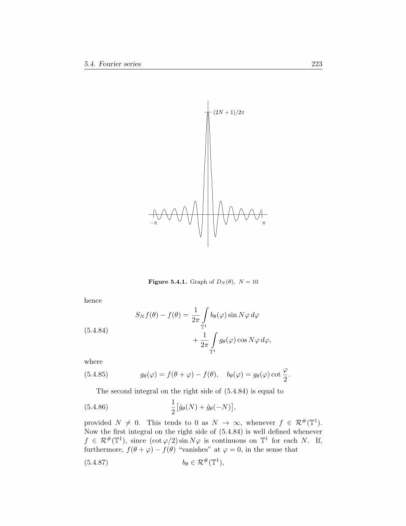
5.4. Fourier series 223
Figure 5.4.1. Graph of DN (θ), N = 10
hence
(5.4.84)
SNf(θ)− f(θ) =1
2π
∫T1
bθ(φ) sinNφdφ
+1
2π
∫T1
gθ(φ) cosNφdφ,
where
(5.4.85) gθ(φ) = f(θ + φ)− f(θ), bθ(φ) = gθ(φ) cotφ
2.
The second integral on the right side of (5.4.84) is equal to
(5.4.86)1
2
[gθ(N) + gθ(−N)
],
provided N = 0. This tends to 0 as N → ∞, whenever f ∈ R#(T1).Now the first integral on the right side of (5.4.84) is well defined wheneverf ∈ R#(T1), since (cotφ/2) sinNφ is continuous on T1 for each N . If,furthermore, f(θ + φ)− f(θ) “vanishes” at φ = 0, in the sense that
(5.4.87) bθ ∈ R#(T1),
224 5. Further Topics in Analysis
then this integral is equal to
(5.4.88)1
2i
[bθ(N)− bθ(−N)
],
which tends to 0 as N → ∞, given (5.4.87). We record the result justestablished.
Proposition 5.4.9. Let f ∈ R#(T1). Fix θ ∈ T1, and define gθ, bθ asin (5.4.85). Assume gθ(φ) “vanishes” at φ = 0, in the sense that (5.4.87)holds. Then
(5.4.89) SNf(θ) −→ f(θ), as N → ∞.
Proposition 5.4.9 has the following application. We say a function f ∈R#(T1) is Holder continuous at θ ∈ T1, with exponent α ∈ (0, 1], providedthere exists δ > 0, C <∞, such that
(5.4.90) |φ| ≤ δ =⇒ |f(θ + φ)− f(θ)| ≤ C|φ|α.
Proposition 5.4.9 implies the following.
Proposition 5.4.10. Let f ∈ R#(T1). If f is Holder continuous at θ, withsome exponent α ∈ (0, 1], then (5.4.89) holds.
Proof. We have
(5.4.91)∣∣∣f(θ + φ)− f(θ)
sinφ/2
∣∣∣ ≤ C ′|φ|−(1−α),
for |φ| ≤ δ. Since sinφ/2 is bounded away from 0 for φ ∈ [−π, π] \ [−δ, δ],the hypothesis (5.4.87) holds.
We now look at the following class of piecewise regular functions, withjumps. Take points pj ,
(5.4.92) −π = p0 < p1 < · · · < pK = π.
Take functions
(5.4.93) fj : [pj , pj+1] −→ C,
Holder continuous with exponent α > 0, for 0 ≤ j ≤ K−1. Define f : T1 →C by
(5.4.94)
f(θ) = fj(θ), if pj < θ < pj+1,
fj(pj+1) + fj+1(pj+1)
2, if θ = pj+1.
By convention, we take K ≡ 0 (recall that π ≡ −π in T1).
Proposition 5.4.11. With f as specified above, we have
(5.4.95) SNf(θ) −→ f(θ), ∀ θ ∈ T1.
5.4. Fourier series 225
Proof. If θ /∈ p0, . . . , pK, this follows from Proposition 5.4.10. It remainsto consider the case θ = pj for some j. Note that
(5.4.96) SNRφf = RφSNf,
where Rφf(θ) = f(θ + φ). Hence there is no loss of generality in takingpj = 0. Parallel to (5.4.96), we have
(5.4.97) SNTf = TSNf, Tf(θ) = f(−θ).
Hence
(5.4.98) SNf(0) =1
2SN (f + Tf)(0).
However, f +Tf is Holder continuous at θ = 0, with value 2f(0), so Propo-sition 5.4.10 implies
(5.4.99)1
2SN (f + Tf)(0) −→ f(0), as N → ∞.
This gives (5.4.95) for θ = pj = 0.
If f is given by (5.4.92)–(5.4.94) and α ∈ (0, 1), we say
(5.4.100) f ∈ PCα(T1).
If instead m ∈ N and such fj in (5.4.93) belong to Cm([pj , pj+1]), we say
(5.4.101) f ∈ PCm(T1).
Let us take a closer look at the following function χ, which belongs toPCm(T1) for all m ∈ N:
(5.4.102)χ(θ) = 0 for − π < θ < 0,
1 for 0 < θ < π,
with χ(0) = χ(±π) = 1/2. A calculation (cf. Exercise 3 below) gives
(5.4.103) χ(0) =1
2, χ(k) =
1
2πi
[1− (−1)k
], k = 0.
Hence
(5.4.104) SNχ(θ) =1
2+
2
π
M∑ℓ=1
sin(2ℓ+ 1)θ
2ℓ+ 1, N = 2M + 1.
See Figures 5.4.2–5.4.3 for the graphs of SNχ(θ), with N = 11 and N = 21.
These graphs illustrate the following phenomena regarding SNχ(θ).
(I) If J is a closed interval in T1 that is disjoint from the points where χjumps, then
(5.4.105) supθ∈J
|SNχ(θ)− χ(θ)| −→ 0, as N → ∞.

226 5. Further Topics in Analysis
Figure 5.4.2. Graph of SNχ(θ), N = 11.
(II) Near a point of discontinuity, SNχ(θ) overshoots χ(θ), by an amountthat does not decay as N → ∞. This overshot is accompanied by an os-cillatory behavior in SNχ(θ), that decays as θ moves away from the jump.
The first phenomenon is a special case of Riemann localization of convergenceof Fourier series. The second is a special case of the Gibbs phenomenon. Weaim to establish some results that justify these observations.
For this, it will be convenient to bring in the following class of functions.
Definition. Given f ∈ R(T1), we say f ∈ BV(T1) provided there existfν ∈ C1(T1) and A <∞ such that
(5.4.106) ∥f ′ν∥L1 ≤ A, and fν → f in L2-norm.
We write
(5.4.107)∥f∥TV = infA : (5.4.106) holds,∥f∥BV = ∥f∥sup + ∥f∥TV.
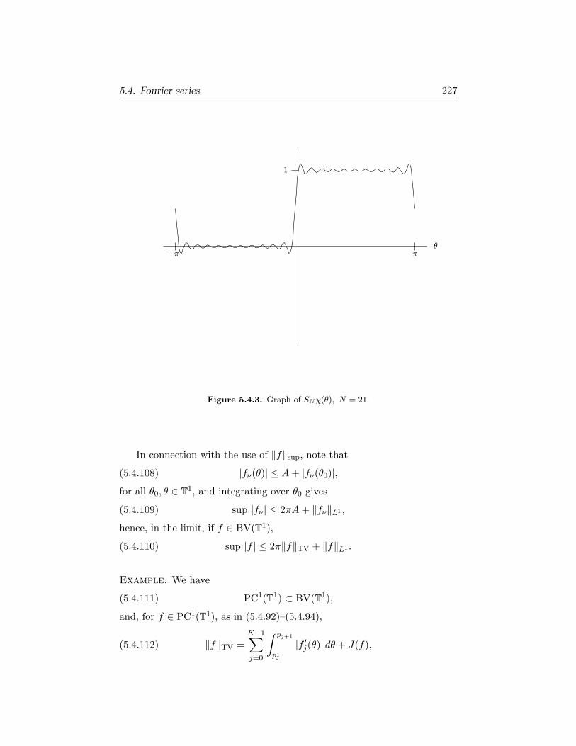
5.4. Fourier series 227
Figure 5.4.3. Graph of SNχ(θ), N = 21.
In connection with the use of ∥f∥sup, note that
(5.4.108) |fν(θ)| ≤ A+ |fν(θ0)|,
for all θ0, θ ∈ T1, and integrating over θ0 gives
(5.4.109) sup |fν | ≤ 2πA+ ∥fν∥L1 ,
hence, in the limit, if f ∈ BV(T1),
(5.4.110) sup |f | ≤ 2π∥f∥TV + ∥f∥L1 .
Example. We have
(5.4.111) PC1(T1) ⊂ BV(T1),
and, for f ∈ PC1(T1), as in (5.4.92)–(5.4.94),
(5.4.112) ∥f∥TV =
K−1∑j=0
∫ pj+1
pj
|f ′j(θ)| dθ + J(f),
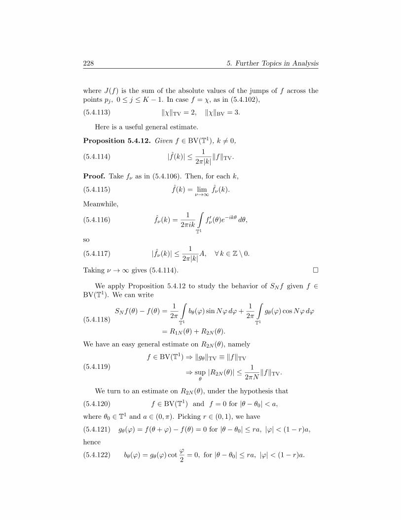
228 5. Further Topics in Analysis
where J(f) is the sum of the absolute values of the jumps of f across thepoints pj , 0 ≤ j ≤ K − 1. In case f = χ, as in (5.4.102),
(5.4.113) ∥χ∥TV = 2, ∥χ∥BV = 3.
Here is a useful general estimate.
Proposition 5.4.12. Given f ∈ BV(T1), k = 0,
(5.4.114) |f(k)| ≤ 1
2π|k|∥f∥TV.
Proof. Take fν as in (5.4.106). Then, for each k,
(5.4.115) f(k) = limν→∞
fν(k).
Meanwhile,
(5.4.116) fν(k) =1
2πik
∫T1
f ′ν(θ)e−ikθ dθ,
so
(5.4.117) |fν(k)| ≤1
2π|k|A, ∀ k ∈ Z \ 0.
Taking ν → ∞ gives (5.4.114).
We apply Proposition 5.4.12 to study the behavior of SNf given f ∈BV(T1). We can write
(5.4.118)SNf(θ)− f(θ) =
1
2π
∫T1
bθ(φ) sinNφdφ+1
2π
∫T1
gθ(φ) cosNφdφ
= R1N (θ) +R2N (θ).
We have an easy general estimate on R2N (θ), namely
(5.4.119)
f ∈ BV(T1) ⇒ ∥gθ∥TV ≡ ∥f∥TV
⇒ supθ
|R2N (θ)| ≤ 1
2πN∥f∥TV.
We turn to an estimate on R2N (θ), under the hypothesis that
(5.4.120) f ∈ BV(T1) and f = 0 for |θ − θ0| < a,
where θ0 ∈ T1 and a ∈ (0, π). Picking r ∈ (0, 1), we have
(5.4.121) gθ(φ) = f(θ + φ)− f(θ) = 0 for |θ − θ0| ≤ ra, |φ| < (1− r)a,
hence
(5.4.122) bθ(φ) = gθ(φ) cotφ
2= 0, for |θ − θ0| ≤ ra, |φ| < (1− r)a.
5.4. Fourier series 229
Since the only singularity of cotφ/2 in T1 is at φ = 0, we have
(5.4.123) bθ ∈ BV(T1), ∀ |θ − θ0| < a,
and
(5.4.124) ∥bθ∥BV ≤ C(r, a)∥f∥BV, for |θ − θ0| ≤ ra,
when r ∈ (0, 1). Hence, by Proposition 5.4.12,
(5.4.125) |R1N (θ)| ≤ C ′(r, a)
N∥f∥BV, for |θ − θ0| ≤ ra,
when (5.4.120) holds. Putting this together with (5.4.119), we have thefollowing.
Proposition 5.4.13. If f ∈ BV(T1) satisfies (5.4.120), then, for each r ∈(0, 1), there exists C = C(r, a) such that
(5.4.126) sup|θ−θ0|≤ra
|SNf(θ)− f(θ)| ≤ C
N∥f∥BV.
We get the same sort of conclusion if (5.4.120) is modified to read
(5.4.127) f ∈ BV(T1), g ∈ C2(T1), and f = g for |θ − θ0| < a,
since g ∈ C2(T1) ⇒ |g(k)| ≤ C/k2. We then replace ∥f∥BV on the rightside of (5.4.126) by ∥f∥BV + ∥g∥C2 . This has the following consequence,explaining Phenomenon I for SNχ(θ).
Corollary 5.4.14. If we take
(5.4.128) f ∈ PC2(T1),
and J is a closed interval in T1 that is disjoint from the set of points wheref has a jump, then there exists C = C(J, f) such that
(5.4.129) supθ∈J
|SNf(θ)− f(θ)| ≤ C
N.
We next address Phenomenon II. We take f ∈ BV(T1) and return to
(5.4.130) SNf(θ) =
∫T1
fθ(φ)DN (φ) dφ, fθ(φ) = f(φ+ θ),
with DN (θ) as in (5.4.83). It will be convenient to relate this to a slightlydifferent family of operators, namely
(5.4.131) SNf(θ) =
∫T1
fθ(φ)EN (φ) dφ,
with
(5.4.132) EN (φ) =1
π
sinNφ
φ.

230 5. Further Topics in Analysis
Note that
(5.4.133) DN (φ) = EN (φ) +1
2πγ(φ) sinNφ+
1
2πcosNφ,
where
(5.4.134) γ(φ) = cotφ
2− 2
φ
is a smooth, odd function of φ on [−π, π] (which, as a function on T1, hasa jump at π). We have
(5.4.135)
∣∣∣ 12π
∫T1
fθ(φ)γ(φ) sinNφdφ∣∣∣ ≤ C
N∥fθγ∥TV
≤ C
N∥f∥BV,
and
(5.4.136)∣∣∣ 12π
∫T1
fθ(φ) cosNφdφ∣∣∣ ≤ C
N∥f∥TV,
hence
(5.4.137) supθ∈T1
∣∣SNf(θ)− SNf(θ)∣∣ ≤ C
N∥f∥BV.
We now specialize to f = χ, given by (5.4.102). We have
(5.4.138) SNχ(θ) =1
π
∫ π−θ
−θ
sinNφ
φdφ, if 0 ≤ θ ≤ π.
Note that
(5.4.139) SNχ(θ)−1
2is odd in θ ∈ [−π, π],
so an analysis of (5.4.138) suffices. Since (sinNφ)/φ is even, we have
(5.4.140) SNχ(θ) =1
π
∫ θ
0
sinNφ
φdφ+
1
π
∫ π−θ
0
sinNφ
φdφ,
for θ ∈ [0, π].
We bring in the following special function:
(5.4.141) G(x) =2
π
∫ x
0
sin y
ydy,
and deduce that
(5.4.142) SNχ(θ) =1
2G(Nθ) +
1
2G(N(π − θ)), for θ ∈ [0, π].

5.4. Fourier series 231
The function G(x) is called the sine-integral. It can be evaluated accu-rately for x in a bounded interval by taking the power series
(5.4.143)sin y
y=
∞∑k=0
(−1)ky2k
(2k + 1)!,
and integrating term by term:
(5.4.144) G(x) =2
π
∞∑k=0
(−1)k
2k + 1
x2k+1
(2k + 1)!.
Regarding the behavior of G(x) as x→ +∞, note that
(5.4.145) G(Nπ) =2
π
N−1∑k=0
(−1)kak,
where
(5.4.146) ak =
∫ (k+1)π
kπ
| sin y|y
dy 0, as k ∞.
It follows that G(x) tends to a finite limit as x→ +∞. In fact,
(5.4.147) limx→∞
G(x) = 1.
This can be seen from
(5.4.148) SNχ(π2
)= G
(Nπ2
), or SNχ(0) =
1
2G(Nπ),
together with (5.4.137) and Proposition 5.4.11, which together imply
(5.4.149) SNχ(π2
)→ χ
(π2
)= 1, SNχ(0) → χ(0) =
1
2, as N → ∞.
From here, another look at (5.4.145)–(5.4.146) yields
(5.4.150) |G(x)− 1| ≤ C
x, for x > 0.
See Exercise 12 below for a more precise result.
See Figure 5.4.4 for the graph of G(x). We see that G(x) overshoots itslimiting value of 1. In fact, as one can check using (5.4.144)–(5.4.146),
(5.4.151) Gmax = G(π) ≈ 1.1789797444 · · · .
Combining the identity (5.4.142) with (5.4.137), we have the followingincisive description of SNχ on [0, π].
Proposition 5.4.15. For χ given by (5.4.102), we have
(5.4.152) sup0≤θ≤π
∣∣∣SNχ(θ)− 1
2
[G(Nθ) +G(N(π − θ))
]∣∣∣ ≤ C
N.
232 5. Further Topics in Analysis
Figure 5.4.4. Graph of the sine-integral, G(x)
We can extend the analysis of Proposition 5.4.15 to negative θ using thefact that both χ(θ)− 1/2 (hence SNχ(θ)− 1/2) and G(x) are odd functionsof their arguments. Combining this observation with Proposition 5.4.15 andwith (5.4.150), we have the following.
Corollary 5.4.16. Let I ⊂ (−π, π) be a closed interval. Then there existsC = C(I) <∞ such that
(5.4.153) supθ∈I
∣∣∣SNχ(θ)− 1
2− 1
2G(Nθ)
∣∣∣ ≤ C
N.
We now move beyond SNχ and examine the Gibbs phenomenon for amore general class of functions with jumps. We take
(5.4.154) f ∈ PC2(T1).
Assume f has a jump at θ = 0, and
(5.4.155) limθ0
f(θ) = 0, limθ0
f(θ) = 1.
Let I ⊂ (−π, π) be a closed interval, containing 0, but disjoint from theother jumps of f . We can write
(5.4.156) f − χ = g + h,
5.4. Fourier series 233
with h ∈ BV(T1), h ≡ 0 on a neighborhood of I, and g satisfying thehypotheses of Proposition 5.4.2. It follows from Propositions 5.4.2 and 5.4.13that
(5.4.157) supθ∈I
∣∣∣SN (g + h)(θ)− g(θ)∣∣∣ ≤ C
N,
hence
(5.4.158) supθ∈I
∣∣∣SN (f − χ)(θ)− (f − χ)(θ)∣∣∣ ≤ C
N.
Combining this with Corollary 5.4.16 yields the following.
Proposition 5.4.17. Assume f ∈ PC2(T1) satisfies (5.4.155), and let I ⊂(−π, π) be a closed interval that is disjoint from the jumps of f other thanat θ = 0. Then
(5.4.159) SNf(θ) =1
2+
1
2G(Nθ) + (f − χ)(θ) +O
( 1
N
),
uniformly in θ ∈ I.
We leave it as an exercise to extend Proposition 5.4.17 to the case where
(5.4.160) limθ0
f(θ) = a, limθ0
f(θ) = b.
Using the fact that SNRφf = RφSNf for φ ∈ T1, one can also analyze theGibbs phenomenon for SNf(θ) near other jumps of f ∈ PC2(T1).
234 5. Further Topics in Analysis
Exercises
1. Prove (5.4.80).
2. Prove (5.4.97).
3. Compute χ(k) when
(5.4.161)χ(θ) = 1 for 0 < θ < π,
0 for − π < θ < 0.
Then use (5.4.60) to obtain another proof of (5.4.22).
4. Apply Proposition 5.4.11 to χ in (5.4.161), when θ = 0, π/2, π. Usethe computation at θ = π/2 to show the following (compare Exercise 31 inChapter 4, §4.5):
π
4= 1− 1
3+
1
5− 1
7+ · · · .
5. Apply (5.4.60) when f(θ) is given by (5.4.16). Use this to show that
∞∑k=1
1
k4=π4
90.
6. Use Proposition 5.4.10 in concert with Proposition 5.4.2 to demonstratethat (5.4.3) holds when f is Lipschitz and piecewise C2 on T1, without re-course to Corollary 5.3.5 (whose proof in §5.3 uses the Stone-Weierstrasstheorem). Use this in turn to prove Proposition 5.4.1, without using Corol-lary 5.3.5.
7. Use the results of Exercise 6 to give a proof of Corollary 5.3.5 that doesnot use the Stone-Weierstrass theorem.Hint. As in the end of the proof of Theorem 5.2.1, each f ∈ C(T1) can beuniformly approximated by a sequence of Lipschitz, piecewise linear func-tions.
Recall that Corollary 5.3.5 states that each f ∈ C(T1) can be uniformlyapproximated by a sequence of finite linear combinations of the functionseikθ, k ∈ Z. The proof given in §5.3 relied on the Weierstrass approximationtheorem, Theorem 5.2.1, which was used in the proof of Theorems 5.3.1 and

5.4. Fourier series 235
5.3.3. Exercise 7 indicates a proof of Corollary 5.3.5 that does not dependon Theorem 5.2.1.
8. Give another proof of Theorem 5.2.1, as a corollary of Corollary 5.3.5.Hint. You can take I = [−π/2, π/2]. Given f ∈ C(I), you can extend itto f ∈ C([−π, π]), vanishing at ±π, and identify such f with an element ofC(T1). Given ε > 0, approximate f uniformly to within ε on [−π, π] by afinite sum
N∑k=−N
akeikθ.
Then approximate eikθ uniformly to within ε/(2N + 1) by a partial sum ofthe power series for eikθ, for each k ∈ −N, . . . , N.
9. Let f ∈ C(T1). Assume there exist fν ∈ A(T1) and B < ∞ such thatfν → f uniformly on T1 and
∞∑k=−∞
|fν(k)| ≤ B, ∀ ν.
Show that f ∈ A(T1).
10. Let f ∈ C(T1). Assume there exist fν ∈ C(T1) satisfying the conditionsof Proposition 5.4.6 such that fν → f uniformly on T1, and assume thereexists C <∞ such that ∫
T1
|f ′ν(θ)|2 dθ ≤ C, ∀ ν.
Show that f ∈ A(T1). Hint. Use (5.4.69), with f replaced by fν .
11. Recall the Dirichlet kernel DN (θ), defined by (5.4.76). Show that
(5.4.162)
DN (θ) =1
2π
N∑k=−N
cos kθ
=1
2π
(1 + 2
N∑k=1
cos kθ).
Try to find trigonometric identities, not involving the complex exponentialseikθ, that take one from (5.4.162) to the key identity (5.4.77), i.e.,
(5.4.163) DN (θ) =1
2π
sin(N + 1/2)θ
sin θ/2.
236 5. Further Topics in Analysis
Remark. One point of this exercise is to highlight the advantages of be-ing able to work with complex-valued functions, which, in (5.4.78)–(5.4.79),allow one to reduce the calculation of DN (θ) to a simple geometric series.The reader is challenged to establish (5.4.163) without benefit of this use ofcomplex numbers. Feel free to throw in the towel if you get stuck!
12. Recall the sine-integral
G(x) =2
π
∫ x
0
sin y
ydy.
Using (5.4.147) and integration by parts, show that, for x > 0,
1−G(x) =2
π
∫ ∞
x
1
ysin y dy
=2
π
[cosxx
−∫ ∞
x
1
y2cos y dy
]=
2
π
[cosxx
− sinx
x2+
∫ ∞
x
2
y3sin y dy
].

5.5. Newton’s method 237
5.5. Newton’s method
Here we describe a method to approximate the solution to
(5.5.1) f(ξ) = 0.
We assume f : [a, b] → R is continuous and f ∈ C2((a, b)). We assumeit is known that f vanishes somewhere in (a, b). For example, f(a) andf(b) might have opposite signs. We take x0 ∈ (a, b) as an initial guess of asolution to (5.5.1), and inductively construct the sequence (xk), going fromxk to xk+1 as follows. Replace f by its best linear approximation at xk,
(5.5.2) g(x) = f(xk) + f ′(xk)(x− xk),
and solve g(xk+1) = 0. This yields
(5.5.3) xk+1 − xk = − f(xk)
f ′(xk),
or
(5.5.4) xk+1 = xk −f(xk)
f ′(xk).
See Figure 5.5.1 for an illustration. Naturally, we need to assume f ′(x)is bounded away from 0 on (a, b). This production of the sequence (xk)is Newton’s method, and as we will see, under appropriate hypotheses itconverges quite rapidly to ξ.
We want to give a condition guaranteeing that |xk+1− ξ| < |xk− ξ|. Say
(5.5.5) xk = ξ + δ.
Then (5.5.4) yields
(5.5.6)
xk+1 − ξ = δ − f(ξ + δ)
f ′(ξ + δ)
=f ′(ξ + δ)δ − f(ξ + δ)
f ′(ξ + δ).
Now the mean value theorem implies
(5.5.7) f(ξ + δ)− f(ξ) = f ′(ξ + τδ)δ, for some τ ∈ (0, 1).
Since f(ξ) = 0, we get from (5.5.6) that
(5.5.8) xk+1 − ξ =f ′(ξ + δ)− f ′(ξ + τδ)
f ′(ξ + δ)δ.
A second application of the mean value theorem gives
(5.5.9) f ′(ξ + δ)− f ′(ξ + τδ) = (1− τ)δf ′′(ξ + γδ),

238 5. Further Topics in Analysis
Figure 5.5.1. One iteration of Newton’s method
for some γ ∈ (τ, 1), hence
(5.5.10) xk+1 − ξ = (1− τ)f ′′(ξ + γδ)
f ′(ξ + δ)δ2, τ ∈ (0, 1), γ ∈ (τ, 1).
Consequently,
(5.5.11) |xk+1 − ξ| ≤ sup0<γ<1
∣∣∣f ′′(ξ + γδ)
f ′(ξ + δ)
∣∣∣δ2.A favorable condition for convergence is that the right side of (5.5.11) is≤ βδ for some β < 1. This leads to the following.
Proposition 5.5.1. Let f ∈ C([a, b]) be C2 on (a, b). Assume there existsa solution ξ ∈ (a, b) to (5.5.1). Assume there exist A,B ∈ (0,∞) such that
(5.5.12) |f ′′(x)| ≤ A, |f ′(x)| ≥ B, ∀x ∈ (a, b).
Pick x0 ∈ (a, b). Assume
(5.5.13) |x0 − ξ| = δ0, [ξ − δ0, ξ + δ0] ⊂ (a, b),
and
(5.5.14)A
Bδ0 = β < 1.
5.5. Newton’s method 239
Then xk, defined inductively by (5.5.4), converges to ξ as k → ∞.
When Proposition 5.5.1 applies, one clearly has
(5.5.15) |xk − ξ| ≤ βkδ0.
In fact, (5.5.11) implies much faster convergence than this. With |xk − ξ| =δk, (5.5.11) implies
(5.5.16) δk+1 ≤A
Bδ2k,
hence
(5.5.17) δ1 ≤A
Bδ20 , δ2 ≤
(AB
)1+2δ40 , δ3 ≤
(AB
)1+2+4δ80 ,
and, inductively,
(5.5.18) δk ≤(AB
)2k−1δ2k0 = β2
k−1δ0,
with β as in (5.5.14). Note that the exponent on β in (5.5.18) is much larger(for moderately large k) than that in (5.5.15). One says the sequence (xk)converges quadratically to the limit ξ, solving (5.5.1). Roughly speaking,xk+1 has twice as many digits of accuracy as xk. We say that Newton’smethod has quadratic convergence
If we change (5.5.1) to
(5.5.19) f(ξ) = y,
then the results above apply to f(x) = f(x)− y, so we get the sequence ofapproximate solutions defined inductively by
(5.5.20) xk+1 = xk −f(xk)− y
f ′(xk),
and the formula (5.5.10) and estimate (5.5.11) remain valid.
As an example, let us take
(5.5.21) f(x) = x2 on [a, b] = [1, 2], γ ∈ (1, 4),
and approximate ξ =√γ, which solves (5.5.19) with y = γ. Note that
f(1) = 1 < γ and f(2) = 4 > γ. In this case, (5.5.20) becomes
(5.5.22)xk+1 = xk −
x2k − γ
2xk
=xk2
+γ
2xk.
Let us pick
(5.5.23) γ = 2, x0 =3
2.
240 5. Further Topics in Analysis
Examining (1.4)2 and (1.5)2, we see that 1.4 <√2 < 1.5. Thus (5.5.13)
holds with δ0 < 1/10. Furthermore, (5.5.12) holds with A = B = 2, so(5.5.14) holds with β < 1/10. Hence, by (5.5.18),
(5.5.24) |xk −√2| ≤ 10−2k .
Explicit computations give
(5.5.25)
x0 = 1.5
x1 = 1.41666666666666
x2 = 1.41421568627451
x3 = 1.41421356237469
x4 = 1.41421356237309.
We have |x24 − 2| ≤ 4 · 10−16, consistent with (5.5.24).
Under certain circumstances, Newton’s method can be even better thanquadratically convergent. This happens when f ′′(ξ) = 0, assuming also thatf is C3. In such a case, the mean value theorem implies
(5.5.26)f ′′(ξ + γδ) = f ′′(ξ + γδ)− f ′′(ξ)
= γδf (3)(ξ + σγδ),
for some σ ∈ (0, 1). Hence, given |xk − ξ| = δk, we get from (5.5.11) that
(5.5.27) |xk+1 − ξ| ≤ sup0<γ<1
∣∣∣f (3)(ξ + γδk)
f ′(ξ + δk)
∣∣∣δ3k.Thus xk → ξ cubically.
Here is an application to the production of a sequence that rapidly con-verges to π, based on
(5.5.28) sinπ = 0.
We take f(x) = sinx. Then f ′′(x) = − sinx, so the considerations aboveapply. The iteration (5.5.4) becomes
(5.5.29) xk+1 = xk −sinxkcosxk
.
If xk = π + δk, note that
(5.5.30) cos(π + δk) = −1 +O(δ2k),
so the iteration
(5.5.31) xk+1 = xk + sinxk

5.5. Newton’s method 241
is also cubically convergent, if x0 is chosen close enough to π. Now, the firstfew terms of the series (5.4.27)–(5.4.31) of Chapter 4, applied to
(5.5.32)π
6=
∫ 1/2
0
dx√1− x2
(cf. Chapter 4, §4.5, Exercise 7, (4.5.48)), yields π = 3.14 · · · . We take
(5.5.33) x0 = 3,
and use the iteration (5.5.31), obtaining
(5.5.34)
x1 = 3.14112000805987
x2 = 3.14159265357220
x3 = 3.14159265358979.
The error π−x2 is < 2·10−11, and all the printed digits of x3 are accurate. Ifthe computation were to higher precision, x3 would approximate π to quitea few more digits.
By contrast, we apply Newton’s method to
(5.5.35) sinπ
6=
1
2
(equivalent to (5.5.32)). In this case, f(x) = sinx/6, and (5.5.20) becomes
(5.5.36) xk+1 = xk − 6sin(xk/6)− 1/2
cos(xk/6).
If we take x0 = 3, as in (5.5.33), the iteration (5.5.36) yields
(5.5.37)
x1 = 3.14066684291090
x2 = 3.14159261236234
x3 = 3.14159265358979.
Note that x1 here is almost as accurate an approximation to π as is x1 in(5.5.34), but x2 here is substantially less accurate than x2 in (5.5.34). Here,x3 has full accuracy, though as noted above, x3 in (5.5.34) could be muchmore accurate if the computation (5.5.31) were done to higher precision.
242 5. Further Topics in Analysis
Exercises
Using a calculator or a computer, implement Newton’s method to get ap-proximate solutions to the following equations.
1. x5 − x3 + 1 = 0.
2. ex = 2x.
3. tanx = x.
4. x log x = 2.
5. xx = 3.
6. Apply Newton’s method to f(x) = 1/x, obtaining the sequence
(5.5.38) xk+1 = 2xk − ax2k
of approximate solutions to f(x) = a. That is, xk → 1/a, if x0 is closeenough. Try this out with a = 3, x0 = 0.3. Note that the right side of(5.5.38) involves only multiplication and subtraction.
7. In light of Exercise 6, consider the following alternative to (5.5.22) as aniteration to approximate
√γ. Pick x0 ≈
√γ, y0 ≈ 1/x0, and set
(5.5.39)
xk+1 =xk2
+γ
2yk,
yk+1/2 = (2− xk+1yk)yk,
yk+1 = (2− xk+1yk+1/2)yk+1/2.
Here the goal is that xk → √γ while yk → 1/xk. Note that (5.5.39) involves
no divisions (except by 2). Try this out with
γ = 2, x0 = 1.5, y0 =2
3,
and compare the speed of convergence with that displayed in (5.5.25).
8. Prove Proposition 5.5.1 when the hypothesis (5.5.13) is replaced by
(5.5.40) |f(x0)| ≤ Bδ0, [x0 − δ0, x0 + δ0] ⊂ (a, b).

5.6. Inner product spaces 243
5.6. Inner product spaces
In §5.4, we have looked at norms and inner products on spaces of functions,such as C(S1) and R(S1), which are vector spaces. Generally, a complexvector space V is a set on which there are operations of vector addition:
(5.6.1) f, g ∈ V =⇒ f + g ∈ V,
and multiplication by an element of C (called scalar multiplication):
(5.6.2) a ∈ C, f ∈ V =⇒ af ∈ V,
satisfying the following properties. For vector addition, we have
(5.6.3) f + g = g+ f, (f + g) + h = f + (g+ h), f +0 = f, f + (−f) = 0.
For multiplication by scalars, we have
(5.6.4) a(bf) = (ab)f, 1 · f = f.
Furthermore, we have two distributive laws:
(5.6.5) a(f + g) = af + ag, (a+ b)f = af + bf.
These properties are readily verified for the function spaces mentioned above.
An inner product on a complex vector space V assigns to elements f, g ∈V the quantity (f, g) ∈ C, in a fashion that obeys the following three rules:
(5.6.6)
(a1f1 + a2f2, g) = a1(f1, g) + a2(f2, g),
(f, g) = (g, f),
(f, f) > 0 unless f = 0.
A vector space equipped with an inner product is called an inner productspace. For example,
(5.6.7) (f, g) =1
2π
∫S1
f(θ)g(θ) dθ
defines an inner product on C(S1), and also on R(S1), where we identifytwo functions that differ only on a set of upper content zero. Similarly,
(5.6.8) (f, g) =
∫ ∞
−∞f(x)g(x) dx
defines an inner product on R(R) (where, again, we identify two functionsthat differ only on a set of upper content zero).
As another example, in we define ℓ2 to consist of sequences (ak)k∈Z suchthat
(5.6.9)∞∑
k=−∞|ak|2 <∞.

244 5. Further Topics in Analysis
An inner product on ℓ2 is given by
(5.6.10)((ak), (bk)
)=
∞∑k=−∞
akbk.
Given an inner product on V , one says the object ∥f∥ defined by
(5.6.11) ∥f∥ =√
(f, f)
is the norm on V associated with the inner product. Generally, a norm onV is a function f 7→ ∥f∥ satisfying
(5.6.12) ∥af∥ = |a| · ∥f∥, a ∈ C, f ∈ V,
(5.6.13) ∥f∥ > 0 unless f = 0,
(5.6.14) ∥f + g∥ ≤ ∥f∥+ ∥g∥.
The property (5.6.14) is called the triangle inequality. A vector spaceequipped with a norm is called a normed vector space. We can define adistance function on such a space by
(5.6.15) d(f, g) = ∥f − g∥.
Properties (5.6.12)–(5.6.14) imply that d : V ×V → [0,∞) makes V a metricspace.
If ∥f∥ is given by (5.6.11), from an inner product satisfying (5.6.6), itis clear that (5.6.12)–(5.6.13) hold, but (5.6.14) requires a demonstration.Note that
(5.6.16)
∥f + g∥2 = (f + g, f + g)
= ∥f∥2 + (f, g) + (g, f) + ∥g∥2
= ∥f∥2 + 2Re(f, g) + ∥g∥2,
while
(5.6.17) (∥f∥+ ∥g∥)2 = ∥f∥2 + 2∥f∥ · ∥g∥+ ∥g∥2.
Thus to establish (5.6.17) it suffices to prove the following, known as Cauchy’sinequality.
Proposition 5.6.1. For any inner product on a vector space V , with ∥f∥defined by (5.6.11),
(5.6.18) |(f, g)| ≤ ∥f∥ · ∥g∥, ∀ f, g ∈ V.
Proof. We start with
(5.6.19) 0 ≤ ∥f − g∥2 = ∥f∥2 − 2Re(f, g) + ∥g∥2,
5.6. Inner product spaces 245
which implies
(5.6.20) 2Re(f, g) ≤ ∥f∥2 + ∥g∥2, ∀ f, g ∈ V.
Replacing f by af for arbitrary a ∈ C of absolute value 1 yields 2Re a(f, g) ≤∥f∥2 + ∥g∥2, for all such a, hence(5.6.21) 2|(f, g)| ≤ ∥f∥2 + ∥g∥2, ∀ f, g ∈ V.
Replacing f by tf and g by t−1g for arbitrary t ∈ (0,∞), we have
(5.6.22) 2|(f, g)| ≤ t2∥f∥2 + t−2∥g∥2, ∀ f, g ∈ V, t ∈ (0,∞).
If we take t2 = ∥g∥/∥f∥, we obtain the desired inequality (5.6.18). Thisassumes f and g are both nonzero, but (5.6.18) is trivial if f or g is 0.
An inner product space V is called a Hilbert space if it is a complete met-ric space, i.e., if every Cauchy sequence (fν) in V has a limit in V . The spaceℓ2 has this completeness property, but C(S1), with inner product (5.6.7),does not, nor does R(S1). Chapter 2 describes a process of constructing thecompletion of a metric space. When appied to an incomplete inner productspace, it produces a Hilbert space. When this process is applied to C(S1),the completion is the space L2(S1). An alternative construction of L2(S1)uses the Lebesgue integral.

Appendix A
Complementary results
Here we present some results that complement material in the main bodyof the text. Appendix A.1 gives a proof of the Fundamental Theorem ofAlgebra, that every nonconstant polynomial has a complex root. AppendixA.2 refines material from Chapter 4 on the power series for (1− x)b, in caseb > 0. This is useful in the proof of the Weierstrass approximation theoremin Chapter 5. Appendix A.3 shows that π2 is irrational. Appendix A.4 dis-cusses a method of numerically evaluating π that goes back to Archimedes.Appendix A.5 discusses calculations of π using arctangents. Appendix A.6treats the power series for tanx, whose coefficients require a more elaboratederivation than those for sinx and cosx. Appendix A.7 discusses a theoremof Abel, giving the optimal condition under which a power series in t withradius of convergence 1 can be shown to converge uniformly in t ∈ [0, 1],as well as related issues regarding convergence of infinite series. AppendixA.8 discusses the existence of continuous functions on R that are nowheredifferentiable.
A.1. The fundamental theorem of algebra
The following result is the fundamental theorem of algebra.
Theorem A.1.1. If p(z) is a nonconstant polynomial (with complex coeffi-cients), then p(z) must have a complex root.
Proof. We have, for some n ≥ 1, an = 0,
(A.1.1)p(z) = anz
n + · · ·+ a1z + a0
= anzn(1 +O(z−1)
), |z| → ∞,
247
248 A. Complementary results
which implies
(A.1.2) lim|z|→∞
|p(z)| = ∞.
Picking R ∈ (0,∞) such that
(A.1.3) inf|z|≥R
|p(z)| > |p(0)|,
we deduce that
(A.1.4) inf|z|≤R
|p(z)| = infz∈C
|p(z)|.
Since DR = z : |z| ≤ R is compact and p is continuous, there existsz0 ∈ DR such that
(A.1.5) |p(z0)| = infz∈C
|p(z)|.
The theorem hence follows from:
Lemma A.1.2. If p(z) is a nonconstant polynomial and (A.1.5) holds, thenp(z0) = 0.
Proof. Suppose to the contrary that
(A.1.6) p(z0) = a = 0.
We can write
(A.1.7) p(z0 + ζ) = a+ q(ζ),
where q(ζ) is a (nonconstant) polynomial in ζ, satisfying q(0) = 0. Hence,for some k ≥ 1 and b = 0, we have q(ζ) = bζk + · · ·+ bnζ
n, i.e.,
(A.1.8) q(ζ) = bζk +O(ζk+1), ζ → 0,
so, uniformly on S1 = ω : |ω| = 1
(A.1.9) p(z0 + εω) = a+ bωkεk +O(εk+1), ε 0.
Pick ω ∈ S1 such that
(A.1.10)b
|b|ωk = − a
|a|,
which is possible since a = 0 and b = 0. In more detail, since−(a/|a|)(|b|/b) ∈S1, Euler’s identity implies
− a
|a||b|b
= eiθ,
for some θ ∈ R, so we can take
ω = eiθ/k.
A.2. More on the power series of (1− x)b 249
Given (A.1.10),
(A.1.11) p(z0 + εω) = a(1−
∣∣∣ ba
∣∣∣εk)+O(εk+1),
which contradicts (A.1.5) for ε > 0 small enough. Thus (A.1.6) is impossible.This proves Lemma A.1.2, hence Theorem A.1.1.
Now that we have shown that p(z) in (A.1.1) must have one root, wecan show it has n roots (counting multiplicity).
Proposition A.1.3. For a polynomial p(z) of degree n, as in (A.1.1), thereexist r1, . . . , rn ∈ C such that
(A.1.12) p(z) = an(z − r1) · · · (z − rn).
Proof. We have shown that p(z) has one root; call it r1. Dividing p(z) byz − r1, we have
(A.1.13) p(z) = (z − r1)p(z) + q,
where p(z) = anzn−1 + · · · + a0 and q is a polynomial of degree < 1, i.e., a
constant. Setting z = r1 in (A.1.13) yields q = 0, so
(A.1.14) p(z) = (z − r1)p(z).
Since p(z) is a polynomial of degree n − 1, the result (A.1.12) follows byinduction on n.
The numbers rj , 1 ≤ j ≤ n, in (A.1.12) are called the roots of p(z). Ifk of them coincide (say with rℓ) we say rℓ is a root of multiplicity k. If rℓ isdistinct from rj for all j = ℓ, we say rℓ is a simple root.
A.2. More on the power series of (1− x)b
In §4.3 of Chapter 4, we showed that
(A.2.1) (1− x)b =∞∑k=0
akk!xk,
for |x| < 1, with
(A.2.2) a0 = 1, ak =
k−1∏ℓ=0
(−b+ ℓ), for k ≥ 1.
There we required b ∈ Q, but in §4.5 of Chapter 4 we defined yb, for y > 0,for all b ∈ R (and for y ≥ 0 if b > 0), and noted that such a result extends.Here, we prove a further result, when b > 0.
250 A. Complementary results
Proposition A.2.1. Given b > 0, ak as in (A.2.2), the identity (A.2.1)holds for x ∈ [−1, 1], and the series converges absolutely and uniformly on[−1, 1].
Proof. Our main task is to show that
(A.2.3)
∞∑k=0
|ak|k!
<∞,
if b > 0. This implies that the right side of (A.2.1) converges absolutely anduniformly on [−1, 1] and its limit, g(x), is continuous on [−1, 1]. We alreadyknow that g(x) = (1 − x)b on (−1, 1), and since both sides are continuouson [−1, 1], the identity also holds at the endpoints. Now, if k − 1 > b,
(A.2.4)akk!
= − b
k
∏1≤ℓ≤b
(1− b
ℓ
) ∏b<ℓ≤k−1
(1− b
ℓ
),
which we write as (B/k)pk, where pk denotes the last product in (A.2.4).Then
(A.2.5)
log pk =∑
b<ℓ≤k−1
log(1− b
ℓ
)≤ −
∑b<ℓ≤k−1
b
ℓ
≤ −b log k + β,
for some β ∈ R. Here, we have used
(A.2.6) log(1− r) < −r, for 0 < r < 1,
and
(A.2.7)
k−1∑ℓ=1
1
ℓ>
∫ k
1
dy
y.
It follows from (A.2.5) that
(A.2.8) pk ≤ e−b log k+β = γk−b,
so
(A.2.9)|ak|k!
≤ |Bγ| k−(1+b),
giving (C.3).
Exercise
A.3. π2 is irrational 251
1. Why did we not put this argument in §4.3 of Chapter 4?Hint. logs
A.3. π2 is irrational
The following proof that π2 is irrational follows a classic argument of I. Niven,[10]. The idea is to consider
(A.3.1) In =
∫ π
0φn(x) sinx dx, φn(x) =
1
n!xn(π − x)n.
Clearly In > 0 for each n ∈ N, and In → 0 very fast, faster than geometri-cally:
(A.3.2) 0 < In <1
n!
(π2
)2n.
The next key fact, to be established below, is that In is a polynomial ofdegree n in π2 with integer coefficients:
(A.3.3) In =
n∑k=0
cnkπ2k, cnk ∈ Z.
Given this it follows readily that π2 is irrational. In fact, if π2 = a/b, a, b ∈N, then
(A.3.4)n∑
k=0
cnka2kb2n−2k = b2nIn.
But the left side of (A.3.4) is an integer for each n, while by the estimate(A.3.2), the right side belongs to the interval (0, 1) for large n, yielding acontradiction. It remains to establish (A.3.3).
A method of computing the integral in (A.3.1), which works for anypolynomial φn(x) is the following. One looks for an antiderivative of theform
(A.3.5) Gn(x) sinx− Fn(x) cosx,
where Fn and Gn are polynomials. One needs
(A.3.6) Gn(x) = F ′n(x), G′
n(x) + Fn(x) = φn(x),
hence
(A.3.7) F ′′n (x) + Fn(x) = φn(x).
252 A. Complementary results
One can exploit the nilpotence of ∂2x on the space of polynomials of degree≤ 2n and set
(A.3.8)
Fn(x) = (I + ∂2x)−1φn(x)
=n∑
k=0
(−1)kφ(2k)n (x).
Then
(A.3.9)d
dx
(F ′n(x) sinx− Fn(x) cosx
)= φn(x) sinx.
Integrating (A.3.9) over x ∈ [0, π] gives
(A.3.10)
∫ π
0φn(x) sinx dx = Fn(0) + Fn(π) = 2Fn(0),
the last identity holding for φn(x) as in (B.1) because then φn(π−x) = φn(x)and hence Fn(π − x) = Fn(x). For the first identity in (A.3.10), we use thedefining property that sinπ = 0 while cosπ = −1.
In light of (A.3.8), to prove (A.3.3) it suffices to establish an analogous
property for φ(2k)n (0). Comparing the binomial formula and Taylor’s formula
for φn(x):
(A.3.11)
φn(x) =1
n!
n∑ℓ=0
(−1)ℓ(n
ℓ
)πn−ℓxn+ℓ, and
φn(x) =
2n∑k=0
1
k!φ(k)n (0)xk,
we see that
(A.3.12) k = n+ ℓ⇒ φ(k)n (0) = (−1)ℓ
(n+ ℓ)!
n!
(n
ℓ
)πn−ℓ,
so
(A.3.13) 2k = n+ ℓ⇒ φ(2k)n (0) = (−1)n
(n+ ℓ)!
n!
(n
ℓ
)π2(k−ℓ).
Of course φ(2k)n (0) = 0 for 2k < n. Clearly the multiple of π2(k−ℓ) in (A.3.13)
is an integer. In fact,
(A.3.14)
(n+ ℓ)!
n!
(n
ℓ
)=
(n+ ℓ)!
n!
n!
ℓ!(n− ℓ)!
=(n+ ℓ)!
n!ℓ!
n!
(n− ℓ)!
=
(n+ ℓ
n
)n(n− 1) · · · (n− ℓ+ 1).
Thus (A.3.3) is established, and the proof that π2 is irrational is complete.
A.4. Archimedes’ approximation to π 253
Remark. A deeper result is that π is transcendental, i.e., it is not the rootof any nontrivial polynomial with rational coefficients. A proof of this canbe found in [8].
A.4. Archimedes’ approximation to π
Here we discuss an approximation to π proposed by Archimedes. It is basedon the fact (known to the ancient Greeks) that the unit disk D = (x, y) ∈R2 : x2 + y2 ≤ 1 has the property
(A.4.1) AreaD = π.
We have not discussed area in this text, but a detailed study is made in thecompanion text [13].
Actually, (A.4.1) was originally the definition of π. Here, we have taken(4.4.32) of Chapter 4 as the definition. To get the equivalence, we appeal tonotions from first-year calculus, giving areas of regions bounded by graphsin terms of integrals. We have
(A.4.2)
AreaD = 2
∫ 1
−1
√1− x2 dx
= 2
∫ π/2
−π/2cos2 θ dθ
=
∫ π/2
−π/2(cos 2θ + 1) dθ
= π.
Here, the second identity follows from the substitution x = sin θ and thethird from the identity
cos 2θ = cos2 θ − sin2 θ = 2 cos2 θ − 1,
a consequence of (4.5.44), with s = t = θ. One can also get (A.4.1) bycomputing areas in polar coordinates (cf. [13]).
We will discuss the approximation of the area of D by that of a sequenceof polygons, roughly in the spirit of Archimedes, but with the advantage ofadvances in calculus, including the power series for sin t. Once we havethe resulting approximations to π, in (A.4.24), we provide two alternativeapproaches, which do not involve the notion of area. One brings in arclength, instead.
From (A.4.1), the method of Archimedes proceeds as follows. If Pn isa regular n-gon inscribed in the unit circle, then AreaPn → π as n → ∞,
254 A. Complementary results
with
(A.4.3) π − c
n2< AreaPn < π.
See (A.4.18)–(A.4.20) below for more on this. Note that such a polygondecomposes into n equal sized isoceles triangles, with two sides of length 1meeting at an angle αn = 2π/n. Such a triangle Tn has
(A.4.4) Area Tn =(sin
αn
2
)(cos
αn
2
)=
1
2sinαn,
so
(A.4.5) AreaPn =n
2sin
2π
n.
One can obtain an inductive formula for AreaPn for n = 2k as follows.Set
(A.4.6) Sk = sin2π
2k, Ck = cos
2π
2k.
Then, for example, S2 = 1, C2 = 0, and
(A.4.7) (Ck+1 + iSk+1)2 = Ck + iSk,
i.e.,
(A.4.8) C2k+1 − S2
k+1 = Ck, 2Ck+1Sk+1 = Sk.
We are in the position of solving
(A.4.9) x2 − y2 = a, 2xy = b,
for x and y, knowing that a ≥ 0, b, x, y > 0. We substitute y = b/2x intothe first equation, obtaining
(A.4.10) x2 − b2
4x2= a,
then set u = x2 and get
(A.4.11) u2 − au− b2
4= 0,
whose positive solution is
(A.4.12) u =a
2+
1
2
√a2 + b2.
Then
(A.4.13) x =√u, y =
b
2√u.
Taking a = Ck, b = Sk, and knowing that C2k + S2
k = 1, we obtain
(A.4.14) Sk+1 =Sk
2√Uk,
A.4. Archimedes’ approximation to π 255
with
(A.4.15) Uk =1 + Ck
2=
1 +√1− S2
k
2.
Then
(A.4.16) AreaP2k = 2k−1 Sk.
Alternatively, with Pk = AreaP2k , we have
(A.4.17) Pk+1 =Pk√Uk.
As we show below, π is approximated to 15 digits of accuracy in 25 iterationsof (A.4.14)–(A.4.17), starting with S2 = 1 and P2 = 2.
First, we take a closer look at the error estimate in (A.4.3). Note that
(A.4.18) π −AreaPn =n
2
(2πn
− sin2π
n
),
and that
(A.4.19) δ − sin δ =δ3
3!− δ5
5!+ · · · < δ3
3!, for 0 < δ < 6,
so
(A.4.20) π −AreaPn <2π3
3· 1
n2, for n ≥ 2.
Thus we can take c = 2π3/3 in (A.4.3) for n ≥ 2, and this is asymptoticallysharp.
From (A.4.20) with n = 225, we have
(A.4.21) π − P25 <2π3
3· 2−50.
Since
(A.4.22) 210 = 1024 ⇒ 250 ≈ 1015, and2π3
3≈ 20,
we get
(A.4.23) π − P25 ≈ 10−14.
We record computations of Pk for k = 5, . . . , 25:
(A.4.24)
P5 = 3.124
P10 = 3.14157
P15 = 3.14159263
P20 = 3.14159265357
P25 = 3.14159265358978.
Note the agreement with (A.4.23).
256 A. Complementary results
The Archimedes method often gets bad press because the error given in(A.4.20) decreases slowly with n. However, given that we take n = 2k anditerate on k, the error actually decreases exponentially in k. Nevertheless,use of the infinite series suggested in Exercise 7 of §4.5 in Chapter 4 hasadvantages over the use of (A.4.14)–(A.4.17), particularly in that it doesnot require one to calculate a bunch of square roots.
There is another disadvantage of the iteration (A.4.14)–(A.4.17), thoughit does not show up in a mere 25 iterations (at least, not if one is using doubleprecision arithmetic). Namely, any error in the approximate calculation ofPk (compared to its exact value), due for example to truncation error, canget magnified in the approximate calculation of Pk+ℓ for ℓ ≥ 1. This willultimately lead to an instability, and a breakdown in the viability of theiterative method (A.4.14)–(A.4.17).
We next show how the approximation to π described here can be justifiedwithout any notion of area. In fact, setting
(A.4.25) An =n
2sin
2π
n,
(cf. (A.4.5)), we get
(A.4.26) 0 < π −An <2π3
3
1
n2, for n ≥ 2,
directly from (A.4.19); cf. (A.4.20). Thus, we can simply set Pk = A2k ,and then the estimates (A.4.21)–(A.4.23) hold, and the iteration (A.4.14)–(A.4.17) works, without recourse to area.
In effect, the previous paragraph took the geometry out of Archimedes’approximation to π. To bring it back, we note the following variant, makinguse of arc length (treated thoroughly in §4.4 of Chapter 4) in place of area.Namely, the perimeter Qn of the regular n-gon Pn is a union of n linesegments, each being the base of an isoceles triangle with two sides of length1, meeting at an angle αn = 2π/n. Hence each such line segment has length2 sinαn/2, so
(A.4.27) ℓ(Qn) = 2n sinπ
n.
The fact that
(A.4.28) ℓ(Qn) −→ 2π, as n→ ∞
follows from the definition (4.4.32) together with Proposition 4.4.1 of Chap-ter 4. Note that (A.4.27) implies
(A.4.29) ℓ(Qn) = 2A2n,
leading us again to Archimedes’ approximation.
A.5. Computing π using arctangents 257
Note. Actually, Archimedes started with the regular hexagon and pro-
ceeded from there to evaluate Pk = AreaP3·2k , for k up to 5. The basiciteration (A.4.7)–(A.4.15) also applies to this case. By (A.4.20),
0 < π −AreaP96 < 0.00225.
Archimedes’ presentation was
3 +10
71< π < 3 +
1
7.
A.5. Computing π using arctangents
In Exercise 3 of §4.5 in Chapter 4, we defined tan t = sin t/ cos t. It is readilyverified (via Exercise 4 of §4.5 in Chapter 4) that
(A.5.1) tan :(−π2,π
2
)−→ R
is one-to-one and onto, with positive derivative, so it has a smooth inverse
(A.5.2) tan−1 : R −→(−π2,π
2
).
It follows from Exercise 5 of §4.5 in Chapter 4 that
(A.5.3) tan−1 x =
∫ x
0
ds
1 + s2.
We can insert the power series for (1 + s2)−1 and integrate term by term toget
(A.5.4) tan−1 x =∞∑k=0
(−1)k
2k + 1x2k+1, if − 1 < x < 1.
This provides a way to obtain rapidly convergent series for π, alternativeto that proposed in Exercise 7 of §4.5 in Chapter 4, which can be called anevaluation of π using the arcsine.
For a first effort, we use
(A.5.5) tanπ
6=
1√3,
which follows from
(A.5.6) sinπ
6=
1
2, cos
π
6=
√3
2⇐⇒ eπi/6 =
√3
2+
1
2i,
compare Exercises 2 and 7 of §4.5 in Chapter 4. Now (A.5.4)–(A.5.5) yield
(A.5.7)π
6=
1√3
∞∑k=0
(−1)k
2k + 1
(13
)k.
258 A. Complementary results
We can compare (A.5.7) with the series (4.5.48) for π. One difference isthe occurrence of the factor 1/
√3, which is irrational. To be sure, it is not
hard to compute√3 to high precision. Compare Exercises 8–10 of §4.3 in
Chapter 4; for a faster method, see Exercise 8 in §1.7. See also the treatmentof Newton’s method in §5.5 of Chapter 5. Nevertheless, the presence of thisirrational factor in (A.5.7) is a bit of a glitch. Another disadvantage of(A.5.7) is that this series converges more slowly than (4.5.48).
We can do better by expressing π as a finite linear combination of termstan−1 xj for certain fairly small rational numbers xj . The key to this is thefollowing formula for tan(a+ b). Using (4.5.44), we have
(A.5.8)
tan(a+ b) =sin(a+ b)
cos(a+ b)=
sin a cos b+ cos a sin b
cos a cos b− sin a sin b
=tan a+ tan b
1− tan a tan b.
Since tanπ/4 = 1, we have, for a, b, a+ b ∈ (−π/2, π/2),
(A.5.9)π
4= a+ b⇐=
tan a+ tan b
1− tan a tan b= 1.
Taking a = tan−1 x, b = tan−1 y gives
(A.5.10)
π
4= tan−1 x+ tan−1 y ⇐= x+ y = 1− xy
⇐= x =1− y
1 + y.
If we set y = 1/2, we get x = 1/3, so
(A.5.11)π
4= tan−1 1
3+ tan−1 1
2.
The power series (A.5.4) for tan−1(1/3) and tan−1(1/2) both converge fasterthan (A.5.7), but that for tan−1(1/2) converges at essentially the same rateas (4.5.48). We might optimise by taking x = y in (A.5.10), but that yieldsx = y =
√2 − 1, and we do not want to plug this irrational number into
(A.5.4). Taking a cue from√2 − 1 ≈ 0.414, we set y = 2/5, which yields
x = 3/7, so
(A.5.12)π
4= tan−1 2
5+ tan−1 3
7.
Both resulting power series converge faster than (4.5.48), but not by much.
To do better, we bring in a formula for tan(a + 2b). Note that settinga = b in (A.5.8) yields
(A.5.13) tan 2b =2 tan b
1− tan2 b,
A.5. Computing π using arctangents 259
and concatenating this with (A.5.8) (with b replaced by 2b) yields, aftersome elementary calculation,
(A.5.14) tan(a+ 2b) =tan a(1− tan2 b) + 2 tan b
1− tan2 b− 2 tan a tan b.
Thus, parallel to (A.5.9),
(A.5.15)π
4= a+ 2b⇐=
tan a(1− tan2 b) + 2 tan b
1− tan2 b− 2 tan a tan b= 1.
Taking a = tan−1 x, b = tan−1 y gives
(A.5.16)
π
4= tan−1 x+ 2 tan−1 y ⇐= x(1− y2) + 2y = 1− y2 − 2xy
⇐= x =1− y2 − 2y
1− y2 + 2y.
Taking y = 1/3 yields x = 1/7, so
(A.5.17)π
4= tan−1 1
7+ 2 tan−1 1
3.
Both resulting power series converge significantly faster than (4.5.48). Al-ternatively, we can take y = 1/4, yielding x = 7/23, so
(A.5.18)π
4= tan−1 7
23+ 2 tan−1 1
4.
The power series for tan−1(7/23) converges a little faster than that fortan−1(1/3).
One can go still farther, iterating (A.5.13) to produce a formula fortan 4b, and concatenating this with (A.5.8) to produce a formula for
(A.5.19) tan(a+ 4b).
An argument somewhat parallel to that involving (A.5.15)–(A.5.16) yieldsidentities of the form
(A.5.20)π
4= tan−1 x+ 4 tan−1 y,
including the following, known as Machin’s formula:
(A.5.21)π
4= 4 tan−1 1
5− tan−1 1
239,
with y = 1/5, x = −1/239. For many years, this was the most popularformula for high precision approximations to π, until the 1970s, when amore sophisticated method (actually discovered by Gauss in 1799) becameavailable. For more on this, the reader can consult Chapter 7 of [1].
Returning to the arctangent function, we record a series that convergessomewhat faster than (A.5.4), for such values of x as occur in (A.5.11),(A.5.12), (A.5.17), (A.5.18), and (A.5.21). The following is due to Euler.

260 A. Complementary results
Proposition A.5.1. For x ∈ R,
(A.5.22) x tan−1 x = φ( x2
1 + x2
),
with
(A.5.23) φ(z) = z(1 +
2
3z +
2 · 43 · 5
z2 +2 · 4 · 63 · 5 · 7
z3 + · · ·).
The power series (A.5.23) has the same radius of convergence as (A.5.4).The advantage of (A.5.22)–(A.5.23) over (A.5.4) lies in the fact that x2/(1+x2) is a bit smaller than x2, for the values of x that appear in our variousformulas for π.
To start the proof of Proposition A.5.1, note that
(A.5.24) z =x2
1 + x2⇐⇒ x2 =
z
1− z.
Hence, by (A.5.4),
(A.5.25)
x tan−1 x =
∞∑k=1
(−1)k−1
2k − 1x2k
=∞∑k=1
(−1)k−1
2k − 1zk(1− z)−k.
Now
(A.5.26) (1− z)−1 =
∞∑n=0
zn,
and differentiating repeatedly gives
(A.5.27) (1− z)−k =∞∑n=0
(k + n− 1
n
)zn,
for |z| < 1. Thus, with z = x2/(1 + x2), we have (A.5.22) with
(A.5.28)
φ(z) =∞∑k=1
∞∑n=0
(−1)k−1
2k − 1
(k + n− 1
n
)zn+k
=
∞∑ℓ=1
ℓ−1∑n=0
(−1)ℓ−n−n
2ℓ− 2n− 1
(ℓ− 1
n
)zℓ.
Hence
(A.5.29) φ(z) =
∞∑ℓ=1
ℓ−1∑m=0
(−1)m
2m+ 1
(ℓ− 1
m
)zℓ.

A.6. Power series for tanx 261
To get (A.5.23), it remains to show that
(A.5.30) φℓ =ℓ−1∑m=0
(−1)m
2m+ 1
(ℓ− 1
m
)=⇒ φℓ =
2 · 4 · · · 2(ℓ− 1)
3 · 5 · · · (2ℓ− 1), ℓ ≥ 2,
while
(A.5.31) φ1 = 1.
In fact, (A.5.31) is routine, so it suffices to establish that
(A.5.32) φℓ+1 =2ℓ
2ℓ+ 1φℓ.
To see this, note that the binomial formula gives
(A.5.33) (1− s2)ℓ−1 =ℓ−1∑m=0
(−1)m(ℓ− 1
m
)s2m,
and integrating over s ∈ [0, 1] gives
(A.5.34) φℓ =
∫ 1
0(1− s2)ℓ−1 ds.
To get the recurrence relation (A.5.32), we start with
(A.5.35)
d
ds(1− s2)ℓ+1 = −2(ℓ+ 1)s(1− s2)ℓ,
d2
ds2(1− s2)ℓ+1 = −2(ℓ+ 1)(1− s2)ℓ + 4ℓ(ℓ+ 1)s2(1− s2)ℓ−1.
Integrating the last identity over s ∈ [0, 1] gives
(A.5.36) 2ℓ
∫ 1
0(1− s2)ℓ−1s2 ds =
∫ 1
0(1− s2)ℓ ds.
Hence
(A.5.37) 2ℓ(−φℓ+1 + φℓ) = φℓ+1,
which gives (A.5.32). This finishes the proof of Proposition A.5.1.
A.6. Power series for tanx
Recall that
(A.6.1) tanx =sinx
cosx
is a smooth function on (−π/2, π/2). Here we desire to represent it as aconvergent power series
(A.6.2) T (x) =
∞∑k=0
τkx2k+1.
262 A. Complementary results
Only odd exponents are involved since tan(−x) = − tanx. We will derive arecursive formula for the coefficients τk.
As seen in Exercise 4 of §4.5 in Chapter 4,
(A.6.3)d
dxtanx = 1 + tan2 x.
To find the coefficients τk in (A.6.2), we construct the power series to solvethe differential equation
(A.6.4) T ′(x) = 1 + T (x)2, T (0) = 0.
Indeed, if (A.6.2) is a convergent power series for |x| < r, then, on such aninterval,
(A.6.5) T ′(x) =∞∑k=0
(2k + 1)τkx2k,
and
(A.6.6)
T (x)2 =∑j,k≥0
τjτkx2(j+k)+2
=∞∑ℓ=0
ℓ∑k=0
τkτℓ−kx2ℓ+2.
We can rewrite (A.6.5) as
(A.6.7) T ′(x) = τ0 +
∞∑ℓ=0
(2ℓ+ 3)τℓ+1x2ℓ+2,
and then the equation (A.6.2) yields τ0 = 1 and
(A.6.8) τℓ+1 =1
2ℓ+ 3
ℓ∑k=0
τkτℓ−k, for ℓ ≥ 0.
Clearly, given τ0 = 1, (A.6.8) uniquely determines τk for all k ∈ N. Thefirst few terms are
(A.6.9) τ0 = 1, τ1 =1
3, τ2 =
2
3 · 5, τ3 =
1
7
( 2
3 · 5+
1
3 · 3+
2
3 · 5
).
An easy induction shows that, for each k ∈ N,
(A.6.10) 0 < τk < 1.
It follows that (A.6.2) is a convergent power series, at least on |x| < 1,and that on this interval the equation (A.6.4) holds. We claim that, on theinterval of convergence,
(A.6.11) T (x) = tanx.
A.6. Power series for tanx 263
For this task, remainder formulas such as (4.3.37) and (4.3.38) are notso convenient, since formulas for high derivatives of tanx become quite un-wieldly. We take another approach, bringing in the function tan−1, intro-duced in (A.5.2)–(A.5.3). If (A.6.2) converges for |x| < r, then
(A.6.12) ψ(x) = tan−1 T (x)
defines a smooth function on (−r, r), and, via (A.5.3) and the chain rule,
(A.6.13) ψ′(x) =T ′(x)
1 + T (x)2= 1.
Since ψ(0) = 0, it follows that ψ(x) = x, hence that T (x) = tanx, so
(A.6.14) tanx =∞∑k=0
τkx2k+1,
with τ0 = 1 and τk for k ∈ N defined recursively by (A.6.8).
As one might expect, the radius of convergence of the power series(A.6.14), seen above to be ≥ 1, is actually π/2. This is conveniently es-tabished using methods of complex analysis, such as treated in [14].
The coefficients τk in the power series for tanx are closely related to theBernoulli numbers Bk, which arise in the power series expansion
(A.6.15)z
ez − 1=
∞∑k=0
Bk
k!zk.
In this case, one can multiply the power series on the right side of (A.6.15)by
(A.6.16)ez − 1
z=
∞∑j=0
zj
(j + 1)!
to get the recursion formula
(A.6.17) B0 = 1,
ℓ−1∑k=0
1
(ℓ− k)!
Bk
k!= 0.
The first few terms are
(A.6.18) B0 = 1, B1 = −1
2, B2 =
1
6, B3 = 0, B4 = − 1
30.
Methods of complex analysis (cf. [14]) show that the power series in (A.6.15)has radius of convergence 2π. It turns out that Bk = 0 for all odd k ≥ 3. Infact, a formula equivalent to (A.6.15) is
(A.6.19)1
2
ez + 1
ez − 1=
1
z+
∞∑k=1
B2k
(2k)!z2k−1.
264 A. Complementary results
It is an exercise to show that the difference between the left side of (A.6.19)and 1/z is odd in z. Now an application of Euler’s formula to (A.6.19) yields
(A.6.20) x cotx =
∞∑k=0
(−1)kB2k
(2k)!(2x)2k.
Furthermore, one can show that
(A.6.21) tanx = cotx− 2 cot 2x,
and then deduce from (A.6.20) that (A.6.14) holds, with
(A.6.22) τk−1 = (−1)k−1 22k(22k − 1)
(2k)!B2k, k ≥ 1.
The fact that τk is positive for each k is equivalent to the fact that B2k ispositive for k odd, and negative for k even (which might take one some effortto glean from (A.6.17)). Note that comparing (A.6.22) and (A.6.10) impliesthat the radius of convergence of the power series in (A.6.19) is at least 4.
For further results, relating (A.6.20) to results connecting the Bernoullinumbers to ζ(2k), defined by
(A.6.23) ζ(2k) =
∞∑n=1
n−2k,
see §6.1 of [14]. One upshot of these results is the identity
(A.6.24) tanπ
2x =
∞∑k=1
τ#k x2k−1, τ#k =
4
π(1− 2−2k)ζ(2k).
A.7. Abel’s power series theorem
In this appendix we prove the following result of Abel and derive someapplications.
Theorem A.7.1. Assume we have a convergent series
(A.7.1)∞∑k=0
ak = A.
Then
(A.7.2) f(r) =∞∑k=0
akrk
converges uniformly on [0, 1], so f ∈ C([0, 1]).
As a warm up, we look at the following somewhat simpler result.
A.7. Abel’s power series theorem 265
Proposition A.7.2. Assume we have an absolutely convergent series
(A.7.3)∞∑k=0
|ak| <∞.
Then the series (G.2) converges uniformly on [−1, 1], so f ∈ C([−1, 1]).
Proof. Writing (A.7.2) as∑∞
k=0 fk(r) with fk(r) = akrk, we have |fk(r)| ≤
|ak| for |r| ≤ 1, so the conclusion follows from the Weierstrass M -test,Proposition 3.2.4 of Chapter 3.
Theorem A.7.1 is much more subtle than Proposition A.7.2. One ingre-dient in the proof is the following summation by parts formula.
Proposition A.7.3. Let (aj) and (bj) be sequences, and let
(A.7.4) sn =n∑
j=0
aj .
If m > n, then
(A.7.5)m∑
k=n+1
akbk = (smbm − snbn+1) +m−1∑
k=n+1
sk(bk − bk+1).
Proof. Write the left side of (A.7.5) as
(A.7.6)m∑
k=n+1
(sk − sk−1)bk.
It is then straightforward to obtain the right side.
Before applying Proposition A.7.3 to the proof of Theorem A.7.1, wenote that, by Proposition 3.3.3 of Chapter 3, the power series (A.7.2) con-verges uniformly on compact subsets of (−1, 1), and defines f ∈ C((−1, 1)).Our task here is to get uniform convergence up to r = 1.
To proceed, we apply (A.7.5) with bk = rk and n + 1 = 0, s−1 = 0, toget
(A.7.7)
m∑k=0
akrk = (1− r)
m−1∑k=0
skrk + smr
m.
266 A. Complementary results
Now, we want to add and subtract a function gm(r), defined for 0 ≤ r < 1by
(A.7.8)
gm(r) = (1− r)
∞∑k=m
skrk
= Arm + (1− r)∞∑
k=m
σkrk,
with A as in (G.1) and
(A.7.9) σk = sk −A −→ 0, as k → ∞.
Note that, for 0 ≤ r < 1, µ ∈ N,
(A.7.10)
(1− r)∣∣∣ ∞∑k=µ
σkrk∣∣∣ ≤ (
supk≥µ
|σk|)(1− r)
∞∑k=µ
rk
=(supk≥µ
|σk|)rµ.
It follows that
(A.7.11) gm(r) = Arm + hm(r)
extends to be continuous on [0, 1] and
(A.7.12) |hm(r)| ≤ supk≥m
|σk|, hm(1) = 0.
Now adding and subtracting gm(r) in (A.7.7) gives
(A.7.13)
m∑k=0
akrk = g0(r) + (sm −A)rm − hm(r),
and this converges uniformly for r ∈ [0, 1] to g0(r). We have Theorem A.7.1,with f(r) = g0(r).
Here is one illustration of Theorem A.7.1. Let ak = (−1)k−1/k, whichproduces a convergent series by the alternating series test (Chapter 1, Propo-sition 1.6.3). By (4.5.47),
(A.7.14)
∞∑k=1
(−1)k−1
krk = log(1 + r),
for |r| < 1. It follows from Theorem A.7.1 that this infinite series convergesuniformly on [0, 1], and hence
(A.7.15)
∞∑k=1
(−1)k−1
k= log 2.
A.7. Abel’s power series theorem 267
See Exercise 30 in §4.5 of Chapter 4 for a more direct approach to (A.7.15),using the special behavior of alternating series. Here is a more substantialgeneralization.
Claim. For all θ ∈ (0, 2π), the series
(A.7.16)
∞∑k=1
eikθ
k= S(θ)
converges.
Given this claim (which we establish below), it follows from TheoremA.7.1 that
(A.7.17) limr1
∞∑k=1
eikθ
krk = S(θ), ∀ θ ∈ (0, 2π).
Note that taking θ = π gives (A.7.15). Incidentally, we mention that thefunction log : (0,∞) → R has a natural extension to
(A.7.18) log : C \ (−∞, 0] −→ C,
and
(A.7.19)∞∑k=1
1
kzk = − log(1− z), for |z| < 1,
from which one can deduce, via Theorem A.7.1, that S(θ) in (A.7.16) satisfies
(A.7.20) S(θ) = − log(1− eiθ), 0 < θ < 2π.
Details on (A.7.18)–(A.7.19) would take us too far into the area of complexanalysis for a treatment here. One can find such material in [14].
We want to establish the convergence of (A.7.16) for θ ∈ (0, 2π). In fact,we prove the following more general result.
Proposition A.7.4. If bk 0, then
(A.7.21)∞∑k=1
bkeikθ = F (θ)
converges for all θ ∈ (0, 2π).
Given Proposition A.7.4, it then follows from Theorem A.7.1 that
(A.7.22) limr1
∞∑k=1
bkrkeikθ = F (θ), ∀ θ ∈ (0, 2π).
In turn, Proposition A.7.4 is a special case of the following more generalresult, known as the Dirichlet test for convergence of an infinite series.

268 A. Complementary results
Proposition A.7.5. If bk 0, ak ∈ C, and there exists B <∞ such that
(A.7.23) sk =
k∑j=1
aj =⇒ |sk| ≤ B, ∀ k ∈ N,
then
(A.7.24)
∞∑k=1
akbk converges.
To apply Proposition A.7.5 to Proposition A.7.4, take ak = eikθ andobserve that
(A.7.25)
k∑j=1
eijθ =1− eikθ
1− eiθeiθ,
which is uniformly bounded (in k) for each θ ∈ (0, 2π).
To prove Proposition A.7.5, we use summation by parts, PropositionA.7.3. We have, via (A.7.5) with n = 0, s0 = 0,
(A.7.26)
m∑k=1
akbk = smbm +
m−1∑k=1
sk(bk − bk+1).
Now, if |sk| ≤ B for all k and bk 0, then
(A.7.27)∞∑k=1
|sk(bk − bk+1)| ≤ B∞∑k=1
(bk − bk+1) = Bb1 <∞,
so the infinite series
(A.7.28)
∞∑k=1
sk(bk − bk+1)
is absolutely convergent, and the convergence of the left side of (A.7.26)readily follows.
A.8. Continuous but nowhere-differentiable functions
It is easy to produce continuous functions that are not differentiable every-where, such as | sinx|, which fails to be differentiable at x = kπ, for k ∈ Z,but is differentiable at all other points. In fact, “most” continuous functionsare nowhere differentiable. We will establish a result along this line in thisappendix.
First we will produce a family of continuous, nowhere-differentiable func-tions, of the form
(A.8.1) φ(x) =
∞∑k=1
αk sin(2πβkx),
A.8. Continuous but nowhere-differentiable functions 269
and more generally of the form
(A.8.2) φ(x) =∞∑k=1
αkψ(βkx) =∞∑k=1
ψk(x),
where ψ : R → R is a continuous function with the following properties:
(A.8.3)
ψ(x+ 1) = ψ(x),
max ψ = 1, min ψ = −1,
Λ(ψ) ≤ L,
where Λ(ψ) denotes the Lipschitz constant of ψ,
(A.8.4) Λ(ψ) = supx =y
∣∣∣ψ(x)− ψ(y)
x− y
∣∣∣.As for the coefficients αk and βk, we will have
(A.8.5) αk 0, βk ∞,
at sufficiently rapid rates, specified below, in (A.8.16). We will establish thefollowing.
Proposition A.8.1. Under the conditions (A.8.2)–(A.8.3), and with αk, βksatisfying (A.8.16) below, φ : R → R is continuous, but, for each ξ ∈ R,
(A.8.6) lim suph→0
∣∣∣φ(ξ)− φ(ξ + h)
h
∣∣∣ = ∞.
Hence φ is nowhere differentiable.
Proof. For each integer n ≥ 2, we divide φ(x) into three parts:
(A.8.7)φ(x) =
n−1∑k=1
ψk(x) + ψn(x) +∞∑
k=n+1
ψk(x)
= Φn(x) + ψn(x) +Rn(x).
Conditions we will place on αk and βk will guarantee that oscillations ofψn over intervals of length 2/βn cannot be cancelled out by oscillations ofΦn +Rn.
To start, since
(A.8.8) Λ(ψk) ≤ αkβkL,
we have
(A.8.9) Λ(Φn) ≤ L
n−1∑k=1
αkβk.
270 A. Complementary results
Meanwhile, for all x,
(A.8.10) |Rn(x)| ≤∞∑n+1
αk.
Now, given ξ ∈ R, set
(A.8.11) In(ξ) = x ∈ R : |x− ξ| ≤ β−1n .
We see from (A.8.3) that
(A.8.12) maxx∈In(ξ)
|ψn(x)− ψn(ξ)| ≥ αn.
Meanwhile, by (A.8.9),
(A.8.13) |Φn(x)− Φn(ξ)| ≤ Lβ−1n
n−1∑k=1
αkβk, ∀x ∈ In(ξ),
and, by (A.8.10),
(A.8.14) |Rn(x)−Rn(ξ)| ≤ 2∞∑
k=n+1
αk, ∀x ∈ In(ξ).
It follows from (A.8.12)–(A.8.14) that
(A.8.15) maxx∈In(ξ)
|φ(x)− φ(ξ)| ≥ αn
2,
provided
(A.8.16)αn
2≥ Lβ−1
n
n−1∑k=1
αkβk + 2
∞∑k=n+1
αk.
Hence, if (A.8.16) holds, then, for each ξ ∈ R,
(A.8.17) sup|x−ξ|≤β−1
n
∣∣∣φ(x)− φ(ξ)
x− ξ
∣∣∣ ≥ αnβn2
,
which gives (A.8.6), since our conditions entail
(A.8.18) αnβn −→ ∞, as n→ ∞.
Note that a sufficient condition for (A.8.16) to hold is that simultane-ously
(A.8.19)∞∑
k=n+1
αk ≤ 1
4αn, and γn ≥ 2L
n−1∑k=1
γk, γk = αkβk.
If, for example, we take
(A.8.20) αk = αk, γk = γk,

A.8. Continuous but nowhere-differentiable functions 271
then the first condition in (A.8.19) holds provided α ≤ 1/5, and the secondcondition in (A.8.19) holds provided γ ≥ 2L+ 1.
To proceed, let us take T = R/Z (a variant of T1 = R/2πZ consideredin §5.4), and consider the space C(T) of real valued continuous functions onT (naturally isomorphic to the space of continuous functions on R that areperiodic of period 1), with sup norm
(A.8.21) ∥f∥sup = supx∈T
|f(x)|.
As seen in §3.4, this is a Banach space, a complete metric space with distancefunction d(f, g) = ∥f − g∥sup. Let us define a subset W ⊂ C(T) satisfying(for f ∈ C(T))
(A.8.22) f ∈ W ⇐⇒ lim supy→0
∣∣∣f(ξ)− f(ξ + y)
y
∣∣∣ = ∞, ∀ ξ ∈ T.
As discussed above, elements f ∈ W are nowhere differentiable. The follow-ing is a simple consequence of Proposition A.8.1.
Corollary A.8.2. The set W is dense in C(T).
Proof. Given g ∈ C(T), ε > 0, we can find h ∈ Lip(T) such that ∥g −h∥sup < ε. Then we can construct φ of the form (A.8.2) (with βk ∈ N) suchthat (A.8.6) holds and ∥φ∥sup < ε. It follows that ∥g − (h + φ)∥sup < 2ε,and of course h+ φ ∈ W.
We want to prove a stronger result, that “most” elements of C(T) belongto W. To get this, let us set, for each N ∈ N,
(A.8.23)LN = f ∈C(T) : ∃ ξ ∈ T such that
|f(ξ)− f(ξ + y)| ≤ N |y|, ∀ y ∈ T.
The following will be a key result.
Lemma A.8.3. For each N ∈ N,
(A.8.24) LN is nowhere dense in C(T).
Note that
(A.8.25) W = C(T) \∪N∈N
LN .
Given Lemma A.8.3, we can deduce from the material in §2.4, on the Bairecategory theorem, the following conclusion.
Theorem A.8.4. The complement in C(T) of the set W, hence of the setof nowhere differentiable functions on T, is a set of first category.

272 A. Complementary results
Proof of Lemma A.8.3. If LN does not satisfy (A.8.24), then its closureLN contains an open set U ⊂ C(T). In turn, by Corollary A.8.2, U containsa function φ satisfying
(A.8.26) lim supy→0
∣∣∣φ(ξ)− φ(ξ + y)
y
∣∣∣ = ∞, ∀ ξ ∈ T.
Since LN ⊃ U ∋ φ, we have fν ∈ LN such that
(A.8.27) fν −→ φ, uniformly on T.By definition of LN , there exist ξν ∈ T such that
(A.8.28) |fν(ξν)− fν(ξν + y)| ≤ N |y|, ∀ y ∈ T.Passing to a subsequence, we can arrange that ξν → ξ ∈ T. Replacing fν(x)by gν(x) = fν(x− (ξ − ξν)), we also have gν → φ uniformly, and
(A.8.29) |gν(ξ)− gν(ξ + y)| ≤ N |y|, ∀ y ∈ T.Then taking ν → ∞ yields
(A.8.30) |φ(ξ)− φ(ξ + y)| ≤ N |y|, ∀ y ∈ T.This contradicts (A.8.26), so we have Lemma A.8.3, and hence TheoremA.8.4.

Bibliography
[1] J. Arndt and C. Haenel, π Unleashed, Springer-Verlag, New York, 2001.
[2] R. Bartle and D. Sherbert, Introduction to Real Analysis, J. Wiley, New York, 1992.
[3] P. Beckmann, A History of π, St. Martin’s Press, New York, 1971.
[4] P. Cohen, Set Theory and the Continuum Hypothesis, Dover, New York, 2008.
[5] K. Devlin, The Joy of Sets: Fundamentals of Contemporary Set Theory, Springer-Verlag, New York, 1993.
[6] G. Folland, Real Analysis: Modern Techniques and Applications, Wiley-Interscience,New York, 1984.
[7] J. Kitchen, Calculus of One Variable, Addison-Wesley, New York, 1968.
[8] S. Lang, Algebra, Addison-Wesley, Reading MA, 1965.
[9] S. Lang, Short Calculus, Springer-Verlag, New York, 2002.
[10] I. Niven, A simple proof that π is irrational, Bull. AMS 53 (1947), 509.
[11] K. Smith, Primer of Modern Analysis, Springer-Verlag, New York, 1983.
[12] M. Taylor, Measure Theory and Integration, American Mathematical Society, Prov-idence RI, 2006.
[13] M. Taylor, Introduction to Analysis in Several Variables (Advanced Calculus), Amer-ican Msthematical Society, Providence RI, to appear.
[14] M. Taylor, Introduction to Complex Analysis, GSM #202, American MathematicalSociety, Providence RI, 2019.
[15] M. Taylor, Partial Differential Equations, Vols. 1–3, Springer-Verlag, New York,1996 (2nd ed., 2011).
[16] M. Taylor, Introduction to Differential Equations, American Mathematical Society,Providence RI, 2011.
[17] M. Taylor, Elementary Differential Geometry, Lecture Notes, 2019.
[18] O. Toeplitz, The Calculus, a Genetic Approach, Univ. of Chicago Press, 1963 (trans-lated from German original).
273

Index
Abel’s theorem, 264absolute value, 21, 57absolutely convergent series, 36, 60,
104, 112, 249accumulation point, 75addition, 3, 10, 17, 29, 56alternating series, 36, 184angle, 61arc length, 161, 165, 188Archimedean property, 19, 32Archimedes’ approach to pi, 253arctangent, 257Arzela-Ascoli theorem, 109associative law, 4, 5, 11
Baire category theorem, 86, 271Banach space, 109, 271Bernoulli numbers, 263bijective, 2binomial formula, 156bisection method, 56Bolzano-Weierstrass theorem, 34, 52, 82bounded sequence, 22
calculus, 117cancellation law, 5, 6, 11, 13, 18Cantor set, 55, 94, 146Card, 47cardinal number, 47Cartesian product, 83Cauchy remainder formula, 153, 158Cauchy sequence, 22, 29, 32, 51, 68, 74Cauchy’s inequality, 67, 221, 244
chain rule, 120, 143
change of variable formula, 143, 161
characteristic function, 133
circle, 161
cis, 60, 178
closed set, 51, 61, 68, 75
closure, 51
closure of a set, 75
commutative law, 4, 5, 11
compact metric space, 80
compact set, 51, 61, 69, 89
complete metric space, 74
completeness property, 33, 51, 68
completion of a metric space, 76
complex conjugate, 57
complex number, 56
composite number, 14
connected, 91
connected space, 75
content, 133
continued fraction, 39
continued fractions, 27
continuous function, 52, 88, 131
continuum hypothesis, 55
convergent sequence, 21, 32, 68
convergent series, 35
convex, 126, 174
convolution, 200
cos, 60, 163, 176
cosh, 180, 181
countable set, 49
curve, 159
275

276 Index
Darboux theorem, 132, 137dense subset, 79derivative, 119, 148diagonal construction, 84, 109differentiable, 119differential equation, 172, 262Dini’s theorem, 101Dirichlet kernel, 222, 235Dirichlet test, 267distance, 67distance function, 74distributive law, 5division, 19dominated convergence theorem, 113,
146, 197dot product, 66
e, 41ellipse, 164equicontinuous, 110equivalence class, 29equivalence relation, 9, 16Euclidean space, 66Euler identity, 61, 176, 183Euler’s formula, 264exp, 173exponential function, 41, 60, 172, 184
finite set, 46Fourier series, 212fundamental theorem of algebra, 247fundamental theorem of arithmetic, 14fundamental theorem of calculus, 135,
143, 149
gamma function, 188generalized mean value theorem, 128,
158geometric series, 37, 102, 236Gibbs phenomenon, 226
Heine-Borel theorem, 54, 81Hilbert space, 245homeomorphism, 90Holder continuous, 224
imaginary part, 57improper integral, 191infimum, 37infinite decimal expansion, 37infinite series, 35, 98infinite set, 47injective, 2
inner product, 216, 243inner product space, 243integer, 9integral, 129integral remainder formula, 152integral test, 145integration by parts, 143interior, 75intermediate value theorem, 53, 91interval, 51, 129inverse function theorem, 122, 128irrational number, 41, 251
Lagrange remainder formula, 153, 158Lebesgue integral, 194, 219Lebesgue measure, 134length, 161liminf, 90limit, 21limsup, 90Lipschitz continuous, 135local maximum, 126, 157local minimum, 125, 157log, 174, 184logarithm, 174lower semicontinuous, 93
Machin’s formula, 259max, 52maximum, 89, 120maxsize, 129mean value theorem, 121, 136, 137, 146,
237metric space, 67, 74, 88min, 52minimum, 89, 120minsize, 131modulus of continuity, 90monotone function, 140monotone sequence, 23multiplication, 3, 10, 17, 29, 56multiplying power series, 104
natural numbers, 2neighborhood, 75Newton’s method, 237norm, 66, 109, 216, 244nowhere-differentiable functions, 268
open set, 51, 61, 68, 75order relation, 6, 12, 19, 31outer measure, 134

Index 277
parabola, 164parametrization by arc length, 161partial derivative, 125partition, 129path-connected, 91Peano arithmetic, 2perfect set, 55pi, 62, 162, 178, 180, 240, 251, 257piecewise constant function, 140polar coordinates, 165polynomial, 42, 247power series, 102, 148, 172, 262power series remainder formula, 152powers, 8prime number, 14principle of induction, 2, 7product rule, 119
quadratic convergence, 239
radius of convergence, 102, 148ratio test, 26, 107, 156, 172rational number, 16real number, 29real part, 57regular pentagon, 63reparametrization, 159Riemann integrable, 130Riemann integral, 129Riemann localization, 226Riemann sum, 133, 159Riemann-Lebesgue lemma, 221
Schroeder-Bernstein theorem, 47sec, 179, 181second derivative, 124, 125separable space, 79sequence, 21sin, 60, 95, 163, 176sine-integral, 231, 236sinh, 180, 181speed, 159square integrable function, 219Stirling’s formula, 190Stone-Weierstrass theorem, 208, 234subsequence, 22subtraction, 12, 19summation by parts, 265supremum, 34supremum property, 34surjective, 2
tan, 168, 179, 181, 262
Taylor’s formula with remainder, 144totally disconnected, 55, 95triangle inequality, 21, 58, 67, 74, 216,
244trigonometric function, 172trigonometric identities, 61trigonometric integral, 186trigonometric polynomial, 211Tychonov’s theorem, 83
unbounded integrable function, 191uncountable set, 49uniform continuity, 90uniform convergence, 97, 249upper semicontinuous, 93
vector space, 243velocity, 159
Weierstrass approximation theorem, 205Weierstrass M test, 99well-ordering property, 7