1

Supplemental Lecture 12

Differential Forms for Physics Students I. Introduction

II. Special Relativity and Electrodynamics

Abstract

In our textbook and in various supplementary lectures, special relativity and electrodynamics

have been presented using the mathematics of vector calculus and tensor analysis. More modern

approaches to these subjects use differential forms. The aim of this lecture is to use differential

forms to unify Maxwell’s equations into two quartets (Gauss’ Law and the Maxwell-Ampere

equations in one case, and the absence of magnetic monopoles and Faraday’s equation in the

other case) as a consequence of Lorentz covariance. We begin with an introduction to the

mathematics of differential forms, exterior products, exterior differentiation, interior products,

the Hodge star operator (duality), the Poincare Lemma and generalized Stoke’s Theorems.

Examples are drawn from three dimensional Euclidean space and four dimensional Minkowski

space time. The electromagnetic field strength differential form is introduced and the

transformation properties of the electric and magnetic fields under Lorentz boosts are obtained.

Maxwell’s equations are discussed in the language of differential forms and comparisons with

tensor analyses are presented. The electromagnetic field strength differential form and the

interior product lead to a formulation of the Lorentz force law which is a manifestly covariant.

This lecture supplements material in the textbook: Special Relativity, Electrodynamics and

General Relativity: From Newton to Einstein (ISBN: 978-0-12-813720-8) by John B. Kogut. The

term “textbook” in these Supplemental Lectures will refer to that work.

Keywords: Differential Forms, Exterior Algebra, Exterior Derivative, Poincare Lemma,

Generalized Stoke’s Theorems, Special Relativity, Lorentz Invariance, Electrodynamics,

Maxwell’s Equations, Lorentz Force Law.

Contents Introduction: Setting the Stage. .................................................................................................................... 2

Exterior Algebra ............................................................................................................................................ 5

The Hodge Star (*) Operator ........................................................................................................................ 9

2

Exterior Derivative ...................................................................................................................................... 13

Mappings and Coordinate Changes ............................................................................................................ 15

The Poincare Lemma and its Converse ....................................................................................................... 16

Special Relativity: Inertial Reference Frames, the Minkowski Metric and Four Vectors ............................ 17

Electromagnetism, Tensors and Forms ....................................................................................................... 19

The Lorentz Force Law and the Interior Product ........................................................................................ 26

Generalized Stoke’s Theorem and Integral Theorems in R3 ....................................................................... 28

References .................................................................................................................................................. 29

Introduction: Setting the Stage.

When we study vector calculus in R3, three dimensional Euclidean space, certain combinations

of derivatives and integrals occur repeatedly. For example, there is the gradient of a function,

∇��⃗ 𝑓𝑓 = �𝜕𝜕𝑥𝑥𝑓𝑓,𝜕𝜕𝑦𝑦𝑓𝑓,𝜕𝜕𝑧𝑧𝑓𝑓�

in Cartesian coordinates where 𝜕𝜕𝑥𝑥𝑓𝑓 is short-hand for 𝜕𝜕𝑓𝑓 𝜕𝜕𝜕𝜕⁄ , etc. and its line integral,

�∇��⃗ 𝑓𝑓 ∙ 𝑑𝑑𝑟𝑟𝑏𝑏

𝑎𝑎

= � �𝜕𝜕𝑥𝑥𝑓𝑓 𝑑𝑑𝜕𝜕 + 𝜕𝜕𝑦𝑦𝑓𝑓 𝑑𝑑𝑑𝑑 + 𝜕𝜕𝑧𝑧𝑓𝑓 𝑑𝑑𝑑𝑑�𝑏𝑏

𝑎𝑎

= 𝑓𝑓�𝑏𝑏�⃗ � − 𝑓𝑓(�⃗�𝑎)

In more generality, we find line integrals and integrands,

� (𝐴𝐴 𝑑𝑑𝜕𝜕 + 𝐵𝐵 𝑑𝑑𝑑𝑑 + 𝐶𝐶 𝑑𝑑𝑑𝑑)𝑏𝑏

𝑎𝑎

where the path between �⃗�𝑎 and 𝑏𝑏�⃗ must be specified, and A, B and C are functions of position and

the integrand is 𝜔𝜔 = 𝐴𝐴 𝑑𝑑𝜕𝜕 + 𝐵𝐵 𝑑𝑑𝑑𝑑 + 𝐶𝐶 𝑑𝑑𝑑𝑑.

There are also surface integrals like those expressing Stoke’s Law of vector calculus,

��∇��⃗ × 𝑉𝑉�⃗ � ∙ 𝑑𝑑�⃗�𝑎𝑆𝑆

= � 𝑉𝑉�⃗ ∙ 𝑑𝑑𝑟𝑟𝜕𝜕𝑆𝑆

3

where S is a compact, smooth simple surface in R3 and 𝜕𝜕𝜕𝜕 is its closed boundary curve. The

surface must be orientable and 𝑑𝑑�⃗�𝑎 is its oriented surface area element at point P,

𝑑𝑑�⃗�𝑎 = 𝑑𝑑𝑟𝑟1 × 𝑑𝑑𝑟𝑟2 = (𝑑𝑑𝑑𝑑1𝑑𝑑𝑑𝑑2 − 𝑑𝑑𝑑𝑑1𝑑𝑑𝑑𝑑2,𝑑𝑑𝑑𝑑1𝑑𝑑𝜕𝜕2 − 𝑑𝑑𝜕𝜕1𝑑𝑑𝑑𝑑2,𝑑𝑑𝜕𝜕1𝑑𝑑𝑑𝑑2 − 𝑑𝑑𝑑𝑑1𝑑𝑑𝜕𝜕2)

where 𝑑𝑑𝑟𝑟1 and 𝑑𝑑𝑟𝑟2 are independent vectors that lie in the surface’s tangent space at the point P.

We see that the Cartesian components of 𝑑𝑑�⃗�𝑎 are anti-symmetric in the indices 1 and 2. Such

quantities will be the building blocks of differential forms, as will be discussed later. Note that

𝑑𝑑�⃗�𝑎 is an axial vector (sometimes called a polar vector in the literature) because it is the cross

product of two vectors. The same comment applies to the curl, ∇��⃗ × 𝑉𝑉�⃗ .

In general, we meet integrals,

�(𝑃𝑃 𝑑𝑑𝑑𝑑𝑑𝑑𝑑𝑑 + 𝑄𝑄 𝑑𝑑𝑑𝑑𝑑𝑑𝜕𝜕 + 𝑅𝑅 𝑑𝑑𝜕𝜕𝑑𝑑𝑑𝑑)

and their integrands, 𝛼𝛼 = 𝑃𝑃 𝑑𝑑𝑑𝑑𝑑𝑑𝑑𝑑 + 𝑄𝑄 𝑑𝑑𝑑𝑑𝑑𝑑𝜕𝜕 + 𝑅𝑅 𝑑𝑑𝜕𝜕𝑑𝑑𝑑𝑑.

There are also volume integrals like the expression of Gauss’ Law,

�∇��⃗ ∙ 𝑉𝑉�⃗ 𝑑𝑑𝑑𝑑℧

= �𝑉𝑉�⃗ ∙ 𝑑𝑑�⃗�𝑎𝜕𝜕℧

where 𝑑𝑑𝑑𝑑 is the element of volume, 𝑑𝑑𝜕𝜕𝑑𝑑𝑑𝑑𝑑𝑑𝑑𝑑 in Cartesian coordinates, and 𝜕𝜕℧ is the oriented

surface of the volume ℧.

In general we meet integrals,

�𝜌𝜌 𝑑𝑑𝜕𝜕𝑑𝑑𝑑𝑑𝑑𝑑𝑑𝑑

and integrands 𝛾𝛾 = 𝜌𝜌 𝑑𝑑𝜕𝜕𝑑𝑑𝑑𝑑𝑑𝑑𝑑𝑑.

When we study vector calculus and electrodynamics, we also discover many vector

identities, like 𝐴𝐴 × �𝐵𝐵�⃗ × 𝐶𝐶� = �𝐴𝐴 ∙ 𝐶𝐶�𝐵𝐵�⃗ − �𝐴𝐴 ∙ 𝐵𝐵�⃗ �𝐶𝐶 ,and some involving differential operators

like grad, curl and div, and we learn many identities among them, like, div curl=0, and curl

grad=0. Many of these results appear related, but the formalism of vector calculus and tensor

analysis doesn’t uncover their systematics. This is where differential forms and exterior algebra

shine! Even more importantly, differential forms have geometric significance so we can use them

4

to find geometric identities that are true in any coordinate system. We have seen how important

this is in special and general relativity as well as in differential geometry. A central idea of

relativity is to express physical relationships free of any particular coordinate system or frame of

reference. We will see that differential forms provide a better language in which to accomplish

this goal.

Let’s look ahead to the content of this lecture to see where we are headed. We will

begin with differential forms in an n-dimensional vector space, L. A r-form will read

𝜔𝜔 =1𝑟𝑟!�𝐴𝐴𝑖𝑖1𝑖𝑖2∙∙∙𝑖𝑖𝑟𝑟 𝑑𝑑𝜕𝜕

𝑖𝑖1 ∧ 𝑑𝑑𝜕𝜕𝑖𝑖2 ∧∙∙∙∧ 𝑑𝑑𝜕𝜕𝑖𝑖𝑟𝑟

where 𝐴𝐴𝑖𝑖1𝑖𝑖2∙∙∙𝑖𝑖𝑟𝑟 is fully anti-symmetric in its indices and each index runs from 1 to n and the

“wedge” operation ∧ is also fully antisymmetric. For example, consider a 2-form in R3,

𝜔𝜔 =12

(𝐴𝐴12 𝑑𝑑𝜕𝜕1 ∧ 𝑑𝑑𝜕𝜕2 + 𝐴𝐴21 𝑑𝑑𝜕𝜕2 ∧ 𝑑𝑑𝜕𝜕1 +⋅⋅⋅)

= 𝐴𝐴12 𝑑𝑑𝜕𝜕1 ∧ 𝑑𝑑𝜕𝜕2 + 𝐴𝐴13 𝑑𝑑𝜕𝜕1 ∧ 𝑑𝑑𝜕𝜕3 + 𝐴𝐴23 𝑑𝑑𝜕𝜕2 ∧ 𝑑𝑑𝜕𝜕3

where we used the anti-symmetry of 𝐴𝐴𝑖𝑖𝑖𝑖 and the ∧ operation to simplify the expression and write

it with only ascending indices. In particular, we used,

𝑑𝑑𝜕𝜕1 ∧ 𝑑𝑑𝜕𝜕2 = −𝑑𝑑𝜕𝜕2 ∧ 𝑑𝑑𝜕𝜕1

where 𝜕𝜕 = (𝜕𝜕1, 𝜕𝜕2, … , 𝜕𝜕𝑛𝑛) is an n dimensional vector, and we noted,

𝑑𝑑𝜕𝜕𝑖𝑖 ∧ 𝑑𝑑𝜕𝜕𝑖𝑖 = 0

We will also find in the lecture that for each r-form 𝜔𝜔, we will associate a (𝑟𝑟 + 1) −form

𝑑𝑑𝜔𝜔 which will satisfy a generalized Stokes integral formula,

∫ 𝜔𝜔 = ∫ 𝑑𝑑𝜔𝜔Σ𝜕𝜕Σ (1)

where Σ will denote an appropriate region (a curve, an oriented surface, a compact volume, etc.)

in the space L and 𝜕𝜕Σ denotes its boundary. In addition, we will also demonstrate Poincare’s

Lemma, 𝑑𝑑𝑑𝑑𝜔𝜔 = 0. We will see that these simple, general expressions capture all the diverse

relations in vector calculus and vector algebra that we have alluded to above! The formalism of

5

differential forms unifies much of what we have derived earlier in a very efficient fashion by

concentrating on the underlying geometric objects involved.

We will illuminate these assertions in the sections below.

The spaces of interest in this lecture will be restricted to Euclidean three space R3, Euclidean n-

dimensional space, Rn, and four dimensional Minkowski space time M4. In later lectures on

differential forms in differential geometry and general relativity we will turn to curved spaces

described by general coordinate systems. Here our goal is limited to the basic ideas of

differential forms, and their applications to special relativity and electrodynamics, Maxwell’s

Equations in particular, in Cartesian coordinates.

Exterior Algebra

Let L be an n-dimensional vector space. Call members of this space 1-forms 𝛼𝛼𝑖𝑖 or 𝛽𝛽𝑖𝑖. Then we

construct new vector spaces called Λ𝑝𝑝𝐿𝐿 using a “wedge product”. Its members are called p-

forms. We take Λ0𝐿𝐿 to be the real numbers R, and Λ1𝐿𝐿 = 𝐿𝐿. Then Λ2𝐿𝐿 consists of sums of the

terms 𝛼𝛼𝑖𝑖⋀𝛽𝛽𝑖𝑖, where the wedge operation ⋀ between 1-forms is given the property,

𝛼𝛼⋀𝛽𝛽 = −𝛽𝛽⋀𝛼𝛼 (2)

and so

𝛼𝛼⋀𝛼𝛼 = 0

The wedge product is also given linearity properties,

𝛼𝛼⋀(𝑏𝑏1𝛽𝛽1 + 𝑏𝑏2𝛽𝛽2) = 𝑏𝑏1𝛼𝛼⋀𝛽𝛽1 + 𝑏𝑏2𝛼𝛼⋀𝛽𝛽2 (3.a)

(𝑎𝑎1𝛼𝛼1 + 𝑎𝑎2𝛼𝛼2)⋀𝛽𝛽 = 𝑎𝑎1𝛼𝛼1⋀𝛽𝛽 + 𝑎𝑎2𝛼𝛼2⋀𝛽𝛽 (3.b)

One calls 𝛼𝛼⋀𝛽𝛽 the “exterior product” of the forms 𝛼𝛼 and 𝛽𝛽.

We can uncover more properties of the space Λ2𝐿𝐿 if we choose a basis of L. Let 𝜎𝜎1,

𝜎𝜎2,…, 𝜎𝜎𝑛𝑛 be a basis of L. Then one can write the general vectors 𝛼𝛼 and 𝛽𝛽 as 𝛼𝛼 = ∑ 𝑎𝑎𝑖𝑖𝜎𝜎𝑖𝑖𝑛𝑛1 and

𝛽𝛽 = ∑ 𝑏𝑏𝑖𝑖𝜎𝜎𝑖𝑖𝑛𝑛1 . Then the exterior product of 𝛼𝛼 and 𝛽𝛽 becomes,

6

𝛼𝛼⋀𝛽𝛽 = �� 𝑎𝑎𝑖𝑖𝜎𝜎𝑖𝑖𝑛𝑛

1�⋀ �� 𝑏𝑏𝑖𝑖𝜎𝜎𝑖𝑖

𝑛𝑛

1� = �𝑎𝑎𝑖𝑖𝑏𝑏𝑖𝑖𝜎𝜎𝑖𝑖 ⋀𝜎𝜎𝑖𝑖

Multiplying out and rearranging,

𝛼𝛼⋀𝛽𝛽 = ��𝑎𝑎𝑖𝑖𝑏𝑏𝑖𝑖 − 𝑎𝑎𝑖𝑖𝑏𝑏𝑖𝑖�𝜎𝜎𝑖𝑖 ⋀𝜎𝜎𝑖𝑖𝑖𝑖<𝑖𝑖

We see that members of the set �𝜎𝜎𝑖𝑖⋀𝜎𝜎𝑖𝑖�, 1 < 𝑖𝑖 < 𝑗𝑗 ≤ 𝑛𝑛, form the basis of Λ2𝐿𝐿. Its dimension is,

dimΛ2𝐿𝐿 =𝑛𝑛(𝑛𝑛 − 1)

2= �𝑛𝑛2�

where we identified the binomial coefficient.

The generalization to Λ𝑝𝑝𝐿𝐿 is clear. A p-form reads �𝛼𝛼1⋀𝛼𝛼2⋀… 𝛼𝛼𝑝𝑝−1⋀𝛼𝛼𝑝𝑝�. We can write each

𝛼𝛼𝑖𝑖 in terms of the basis (𝜎𝜎1,𝜎𝜎2, … ,𝜎𝜎𝑛𝑛) of L. The basis of Λ𝑝𝑝𝐿𝐿 is then,

𝜎𝜎𝐻𝐻 = 𝜎𝜎ℎ1 ⋀𝜎𝜎ℎ2⋀…⋀𝜎𝜎ℎ𝑛𝑛

with 1 < ℎ1 < ℎ2 ∙∙∙< ℎ𝑝𝑝 ≤ 𝑛𝑛. So,

dimΛ𝑝𝑝𝐿𝐿 =𝑛𝑛!

𝑝𝑝! (𝑛𝑛 − 𝑝𝑝)!= �

𝑛𝑛𝑝𝑝�

where we again identified the binomial coefficient. Note that dimΛ0𝐿𝐿 = dimΛ𝑛𝑛𝐿𝐿 = 1. The

systematics are important here. Take n=4. Then �40� = 1, �4

1� = 4, �42� = 6, �4

3� = 4 and �44� =

1. This reminds us of the symmetry,

�𝑛𝑛𝑝𝑝� = �

𝑛𝑛𝑛𝑛 − 𝑝𝑝�

This equality will play an important role when we discuss the Hodge star (*) operation in

Minkowski space. We will see later that the relation �42� = 6 implies that the electromagnetic

field provides a six dimensional representation of the Lorentz group. We saw this in the textbook

in our tensor analysis discussion of the electromagnetic field.

Similarly for n=3, �30� = 1, �3

1� = 3, �32� = 3, �3

3� = 1. The relation �32� = 3 will play

an important role in identifying 2-forms in R3 with axial vectors, such as the magnetic field and it

7

will guide us toward constructing a Lorentz invariant 2-form to describe the electromagnetic

field in special relativity.

In more generality we can consider the construction of forms by taking the product of

linear spaces. Consider,

Λ𝑝𝑝𝐿𝐿 × Λ𝑞𝑞𝐿𝐿 → Λ𝑝𝑝+𝑞𝑞𝐿𝐿

with the product �𝛼𝛼1⋀𝛼𝛼2⋀… 𝛼𝛼𝑝𝑝−1⋀𝛼𝛼𝑝𝑝�⋀� 𝛽𝛽1⋀𝛽𝛽2⋀… 𝛽𝛽𝑞𝑞−1⋀𝛽𝛽𝑞𝑞�. The exterior product has the

properties,

1. 𝛼𝛼⋀(𝛽𝛽1 + 𝛽𝛽2) = 𝛼𝛼⋀𝛽𝛽1 + 𝛼𝛼⋀𝛽𝛽2, is distributive

2. 𝛼𝛼⋀(𝛽𝛽⋀𝛾𝛾) = (𝛼𝛼⋀𝛽𝛽)⋀𝛾𝛾, is associative (4)

3. 𝛼𝛼⋀𝛽𝛽 = (−1)𝑝𝑝𝑞𝑞𝛽𝛽⋀𝛼𝛼, where 𝛼𝛼 ∈ Λ𝑝𝑝𝐿𝐿 and 𝛽𝛽 ∈ Λ𝑞𝑞𝐿𝐿

Note that the associative property #2 is not shared by the cross product in three dimensions. For

example, for the usual unit vectors, 𝚤𝚤̂ × �𝚤𝚤̂ × 𝑘𝑘�� ≠ (𝚤𝚤̂ × 𝚤𝚤̂) × 𝑘𝑘�. And to prove property #3, one

simply counts the number of interchanges of the 1-forms to transform 𝛼𝛼⋀𝛽𝛽 to 𝛽𝛽⋀𝛼𝛼.

Let’s demonstrate property #3 through a few examples, a 1-form and a 3-form,

(𝛼𝛼1⋀𝛼𝛼2⋀𝛼𝛼3)⋀𝛽𝛽 = −1 ∙ 𝛼𝛼1⋀𝛼𝛼2⋀𝛽𝛽⋀𝛼𝛼3 = (−1)2𝛼𝛼1⋀𝛽𝛽⋀𝛼𝛼2⋀𝛼𝛼3 = (−1)3𝛽𝛽⋀𝛼𝛼1⋀𝛼𝛼2⋀𝛼𝛼3

By contrast, two 2-forms,

(𝛼𝛼1⋀𝛼𝛼2)⋀(𝛽𝛽1⋀𝛽𝛽2) = (−1)2∙2(𝛽𝛽1⋀𝛽𝛽2)⋀(𝛼𝛼1⋀𝛼𝛼2) = (𝛽𝛽1⋀𝛽𝛽2)⋀(𝛼𝛼1⋀𝛼𝛼2)

Next, let’s take the wedge product of two differential forms in R3,

(𝐴𝐴1 𝑑𝑑𝜕𝜕 + 𝐴𝐴2 𝑑𝑑𝑑𝑑 + 𝐴𝐴3 𝑑𝑑𝑑𝑑)⋀(𝐵𝐵1 𝑑𝑑𝜕𝜕 + 𝐵𝐵2 𝑑𝑑𝑑𝑑 + 𝐵𝐵3 𝑑𝑑𝑑𝑑)

= (𝐴𝐴2𝐵𝐵3 − 𝐴𝐴3𝐵𝐵2)𝑑𝑑𝑑𝑑⋀𝑑𝑑𝑑𝑑 + (𝐴𝐴3𝐵𝐵1 − 𝐴𝐴1𝐵𝐵3)𝑑𝑑𝑑𝑑⋀𝑑𝑑𝜕𝜕 + (𝐴𝐴1𝐵𝐵2 − 𝐴𝐴2𝐵𝐵1)𝑑𝑑𝜕𝜕⋀𝑑𝑑𝑑𝑑 (5)

We see the components of the cross product of the two Cartesian vectors 𝐴𝐴 and 𝐵𝐵�⃗ on the right

hand side. But what are we to make of the differentials? Take the vector of differentials

(𝑑𝑑𝜕𝜕,𝑑𝑑𝑑𝑑,𝑑𝑑𝑑𝑑) and consider {(𝑑𝑑𝜕𝜕, 0,0), (0,𝑑𝑑𝑑𝑑, 0), (0,0,𝑑𝑑𝑑𝑑)} as the basis vectors for 𝐿𝐿 = Λ1𝐿𝐿 . But

we saw above that Λ2𝐿𝐿 is also three dimensional and so there are three independent 2-forms

which can be taken as a basis for Λ2𝐿𝐿: {(𝑑𝑑𝑑𝑑⋀𝑑𝑑𝑑𝑑, 0,0), (0,𝑑𝑑𝑑𝑑⋀𝑑𝑑𝜕𝜕, 0), (0,0,𝑑𝑑𝜕𝜕⋀𝑑𝑑𝑑𝑑)}. From this

8

perspective Eq. 5 gives precisely the cross product of two vectors in R3. But it has the advantages

that 1. It generalizes to all dimensions, and 2. It distinguishes axial vectors from ordinary

vectors. Property #2 here will be important when we consider the magnetic field in Minkowski

space time.

If we take the wedge product between a 1-form and a 2-form, we can retrieve the formula for the

inner product of two vectors,

(𝐴𝐴1 𝑑𝑑𝜕𝜕 + 𝐴𝐴2 𝑑𝑑𝑑𝑑 + 𝐴𝐴3 𝑑𝑑𝑑𝑑)⋀(𝐵𝐵1𝑑𝑑𝑑𝑑⋀𝑑𝑑𝑑𝑑 + 𝐵𝐵2𝑑𝑑𝑑𝑑⋀𝑑𝑑𝜕𝜕 + 𝐵𝐵3𝑑𝑑𝜕𝜕⋀𝑑𝑑𝑑𝑑)

= (𝐴𝐴1𝐵𝐵1 + 𝐴𝐴2𝐵𝐵2 + 𝐴𝐴3𝐵𝐵3)𝑑𝑑𝜕𝜕⋀𝑑𝑑𝑑𝑑⋀𝑑𝑑𝑑𝑑

Note that the right hand side is proportional to the volume 3-form which spans the one

dimensional space Λ3𝐿𝐿, where L is R3 and the inner product of the two vectors 𝐴𝐴 and 𝐵𝐵�⃗ is

𝐴𝐴 ∙ 𝐵𝐵�⃗ = 𝐴𝐴1𝐵𝐵1 + 𝐴𝐴2𝐵𝐵2 + 𝐴𝐴3𝐵𝐵3.

There are other properties of wedge products that play a role in mathematics and physics.

A particularly useful one is the relationship of wedge products to determinants. Let A be a linear

operator with a matrix representation on L,

𝐴𝐴𝜎𝜎𝑖𝑖 = �𝐴𝐴 𝑖𝑖𝑖𝑖

𝑛𝑛

𝑖𝑖=1

𝜎𝜎𝑖𝑖

Then one can derive a formula for the 𝑛𝑛 × 𝑛𝑛 determinant of 𝐴𝐴,

𝐴𝐴𝜎𝜎1 ⋀𝐴𝐴𝜎𝜎2 …⋀𝐴𝐴𝜎𝜎𝑛𝑛 = 𝐷𝐷𝐷𝐷𝐷𝐷(𝐴𝐴) 𝜎𝜎1 ⋀𝜎𝜎2 …⋀𝜎𝜎𝑛𝑛

If we check this formula for the case n=2, we will see how to get the general result,

𝐴𝐴𝜎𝜎1 ⋀𝐴𝐴𝜎𝜎2 = (𝐴𝐴11𝜎𝜎1 + 𝐴𝐴21𝜎𝜎2) ⋀(𝐴𝐴12𝜎𝜎1 + 𝐴𝐴22𝜎𝜎2) = (𝐴𝐴11𝐴𝐴22 − 𝐴𝐴21𝐴𝐴12 ) 𝜎𝜎1 ⋀𝜎𝜎2

where we see the determinant of the 2 × 2 matrix A,

𝐴𝐴 = �𝐴𝐴 11 𝐴𝐴 2

1

𝐴𝐴 12 𝐴𝐴 2

2 �

It should be clear that much of what we have done here does not depend on a metric, or

inner product, for the linear space L. However, we are headed for physical applications. The

inner product for R3, which we have illustrated above is the usual,

9

𝛼𝛼 ∙ 𝛽𝛽 = 𝑎𝑎1𝑏𝑏1 + 𝑎𝑎2𝑏𝑏2 + 𝑎𝑎3𝑏𝑏3

where 𝛼𝛼 = ∑ 𝑎𝑎𝑖𝑖𝜎𝜎𝑖𝑖31 and 𝛽𝛽 = ∑ 𝑏𝑏𝑖𝑖𝜎𝜎𝑖𝑖3

1 .

When we turn to special relativity, the metric becomes pseudo-Riemannian,

𝛼𝛼 ∙ 𝛽𝛽 = −𝑎𝑎0𝑏𝑏0 + 𝑎𝑎1𝑏𝑏1 + 𝑎𝑎2𝑏𝑏2 + 𝑎𝑎3𝑏𝑏3

Note that we have switched the sign of the Minkowski metric relative to the textbook. Clearly

here we want the signature of the metric to be (−, +, +, +) to emphasize the positive definite

aspect of the metric in the spatial subspace R3.

The Hodge Star (*) Operator

We noted above that if L has dimension n, the dimension of Λ𝑝𝑝𝐿𝐿 and Λ𝑛𝑛−𝑝𝑝𝐿𝐿 are identical. This

suggests that we can map forms between the two spaces and maintain the orientation of the basis

vectors when doing so. We considered an example above for 𝑝𝑝 = 1, and 𝑛𝑛 = 3,

(𝐴𝐴1 𝑑𝑑𝜕𝜕 + 𝐴𝐴2 𝑑𝑑𝑑𝑑 + 𝐴𝐴3 𝑑𝑑𝑑𝑑)⋀(𝐵𝐵1𝑑𝑑𝑑𝑑⋀𝑑𝑑𝑑𝑑 + 𝐵𝐵2𝑑𝑑𝑑𝑑⋀𝑑𝑑𝜕𝜕 + 𝐵𝐵3𝑑𝑑𝜕𝜕⋀𝑑𝑑𝑑𝑑)

= (𝐴𝐴1𝐵𝐵1 + 𝐴𝐴2𝐵𝐵2 + 𝐴𝐴3𝐵𝐵3)𝑑𝑑𝜕𝜕⋀𝑑𝑑𝑑𝑑⋀𝑑𝑑𝑑𝑑

This relation also suggests that one can think of the vector 𝐵𝐵�⃗ as existing in Λ1𝐿𝐿 =L instead of Λ2𝐿𝐿

and one can map 2-forms to 1-forms for 𝑛𝑛 = 3. This is the idea behind the definition of the

Hodge star (*) operation.

To begin we provide Λ1𝐿𝐿 = 𝐿𝐿 with an inner product, 𝛼𝛼𝑖𝑖 ∙ 𝛽𝛽𝑖𝑖. This induces an inner product in the

spaces Λ𝑝𝑝𝐿𝐿, �𝛼𝛼1⋀𝛼𝛼2⋀… 𝛼𝛼𝑝𝑝−1⋀𝛼𝛼𝑝𝑝� ∙ � 𝛽𝛽1⋀𝛽𝛽2⋀… 𝛽𝛽𝑝𝑝−1⋀𝛽𝛽𝑝𝑝�. Because of the anti-symmetric

character of the wedge operator, the induced dot product must be anti-symmetric in the indices of

𝛼𝛼𝑖𝑖 and 𝛽𝛽𝑖𝑖. This suggests the definition as a determinant of a 𝑛𝑛 × 𝑛𝑛 matrix,

�𝛼𝛼1⋀𝛼𝛼2⋀… 𝛼𝛼𝑝𝑝−1⋀𝛼𝛼𝑝𝑝� ∙ � 𝛽𝛽1⋀𝛽𝛽2⋀… 𝛽𝛽𝑝𝑝−1⋀𝛽𝛽𝑝𝑝� = 𝑑𝑑𝐷𝐷𝐷𝐷�𝛼𝛼𝑖𝑖 ∙ 𝛽𝛽𝑖𝑖�

In addition to the correct anti-symmetry in the indices i and j, the determinant is unchanged by

interchanging the 𝛼𝛼′𝑠𝑠 and 𝛽𝛽′𝑠𝑠 since this operation merely interchanges rows with columns in the

𝑛𝑛 × 𝑛𝑛 matrix. Take an example, 𝑝𝑝 = 2,

(𝛼𝛼1⋀𝛼𝛼2) ∙ ( 𝛽𝛽1⋀𝛽𝛽2) = 𝑑𝑑𝐷𝐷𝐷𝐷�𝛼𝛼𝑖𝑖 ∙ 𝛽𝛽𝑖𝑖� = (𝛼𝛼1 ∙ 𝛽𝛽1𝛼𝛼2 ∙ 𝛽𝛽2 − 𝛼𝛼1 ∙ 𝛽𝛽2𝛼𝛼2 ∙ 𝛽𝛽1)

10

Now we can define the Hodge star (*) operation: Let L be a linear space of dimension n

with an inner product. Let 𝜏𝜏 ∈ ⋀𝑝𝑝𝐿𝐿 and 𝜇𝜇 ∈ ⋀𝑛𝑛−𝑝𝑝𝐿𝐿. Then ∗ 𝜏𝜏 ∈ ⋀𝑛𝑛−𝑝𝑝𝐿𝐿 is defined so that,

𝜏𝜏⋀𝜇𝜇 = (∗ 𝜏𝜏 ∙ 𝜇𝜇)𝜎𝜎 (6)

where 𝜎𝜎 is the basis form of ⋀𝑛𝑛𝐿𝐿 and the ∙ indicates the inner product in the space ⋀𝑛𝑛−𝑝𝑝𝐿𝐿.

This definition is an obvious generalization of our R3 example. Using it, we can see how *

maps the various differential forms in ⋀𝑛𝑛−𝑝𝑝𝐿𝐿 for the case L=R3. We learn from the R3 example

above,

(𝐴𝐴1 𝑑𝑑𝜕𝜕 + 𝐴𝐴2 𝑑𝑑𝑑𝑑 + 𝐴𝐴3 𝑑𝑑𝑑𝑑)⋀(𝐵𝐵1𝑑𝑑𝑑𝑑⋀𝑑𝑑𝑑𝑑 + 𝐵𝐵2𝑑𝑑𝑑𝑑⋀𝑑𝑑𝜕𝜕 + 𝐵𝐵3𝑑𝑑𝜕𝜕⋀𝑑𝑑𝑑𝑑)

= (𝐴𝐴1𝐵𝐵1 + 𝐴𝐴2𝐵𝐵2 + 𝐴𝐴3𝐵𝐵3)𝑑𝑑𝜕𝜕⋀𝑑𝑑𝑑𝑑⋀𝑑𝑑𝑑𝑑

that,

∗ 𝑑𝑑𝜕𝜕 = 𝑑𝑑𝑑𝑑⋀𝑑𝑑𝑑𝑑, ∗ 𝑑𝑑𝑑𝑑 = 𝑑𝑑𝑑𝑑⋀𝑑𝑑𝜕𝜕, ∗ 𝑑𝑑𝑑𝑑 = 𝑑𝑑𝜕𝜕⋀𝑑𝑑𝑑𝑑

And if we consider the identity,

(𝐵𝐵1𝑑𝑑𝑑𝑑⋀𝑑𝑑𝑑𝑑 + 𝐵𝐵2𝑑𝑑𝑑𝑑⋀𝑑𝑑𝜕𝜕 + 𝐵𝐵3𝑑𝑑𝜕𝜕⋀𝑑𝑑𝑑𝑑)⋀(𝐴𝐴1 𝑑𝑑𝜕𝜕 + 𝐴𝐴2 𝑑𝑑𝑑𝑑 + 𝐴𝐴3 𝑑𝑑𝑑𝑑)

= (𝐴𝐴1𝐵𝐵1 + 𝐴𝐴2𝐵𝐵2 + 𝐴𝐴3𝐵𝐵3)𝑑𝑑𝜕𝜕⋀𝑑𝑑𝑑𝑑⋀𝑑𝑑𝑑𝑑

we also learn that,

∗ (𝑑𝑑𝑑𝑑⋀𝑑𝑑𝑑𝑑) = 𝑑𝑑𝜕𝜕, ∗ (𝑑𝑑𝑑𝑑⋀𝑑𝑑𝜕𝜕) = 𝑑𝑑𝑑𝑑, ∗ (𝑑𝑑𝜕𝜕⋀𝑑𝑑𝑑𝑑) = 𝑑𝑑𝑑𝑑

And finally, ∗∗= 1 for R3.

Next we need the Hodge star (*) operation for Minkowski space time. We choose the basis

{𝑐𝑐𝑑𝑑𝐷𝐷,𝑑𝑑𝜕𝜕1,𝑑𝑑𝜕𝜕2,𝑑𝑑𝜕𝜕3} with the diagonal inner products �𝑑𝑑𝜕𝜕𝑖𝑖 ∙ 𝑑𝑑𝜕𝜕𝑖𝑖� = 1 and (𝑐𝑐𝑑𝑑𝐷𝐷 ∙ 𝑐𝑐𝑑𝑑𝐷𝐷) = −1.

The minus sign in this metric will require attention.

Let’s first obtain ∗ (𝑑𝑑𝜕𝜕⋀𝑑𝑑𝑑𝑑). We begin with a triviality, which is just the definition of 𝜎𝜎,

the basis form for ⋀4𝐿𝐿 for 𝐿𝐿 = M4, 𝜎𝜎 ≡ 𝑐𝑐𝑑𝑑𝐷𝐷⋀𝑑𝑑𝜕𝜕⋀𝑑𝑑𝑑𝑑⋀𝑑𝑑𝑑𝑑, or

(𝑑𝑑𝜕𝜕⋀𝑑𝑑𝑑𝑑)⋀(𝑑𝑑𝑑𝑑⋀𝑐𝑐𝑑𝑑𝐷𝐷) = − 𝜎𝜎

But the relation that defines the Hodge star operator reads,

11

(𝑑𝑑𝜕𝜕⋀𝑑𝑑𝑑𝑑)⋀(𝑑𝑑𝑑𝑑⋀𝑐𝑐𝑑𝑑𝐷𝐷) = �∗ (𝑑𝑑𝜕𝜕⋀𝑑𝑑𝑑𝑑) ∙ (𝑑𝑑𝑑𝑑⋀𝑐𝑐𝑑𝑑𝐷𝐷)� 𝜎𝜎 = − 𝜎𝜎

So,

∗ (𝑑𝑑𝜕𝜕⋀𝑑𝑑𝑑𝑑) ∙ (𝑑𝑑𝑑𝑑⋀𝑐𝑐𝑑𝑑𝐷𝐷) = −1

And this requires ∗ (𝑑𝑑𝜕𝜕⋀𝑑𝑑𝑑𝑑) = 𝑑𝑑𝑑𝑑⋀𝑐𝑐𝑑𝑑t, because the definition of the inner product for ⋀2𝑀𝑀4

reads,

(𝑑𝑑𝑑𝑑⋀𝑐𝑐𝑑𝑑𝐷𝐷) ∙ (𝑑𝑑𝑑𝑑⋀𝑐𝑐𝑑𝑑𝐷𝐷) = det(𝑑𝑑𝑑𝑑 ∙ 𝑑𝑑𝑑𝑑 𝑐𝑐𝑑𝑑𝐷𝐷 ∙ 𝑐𝑐𝑑𝑑𝐷𝐷 − (𝑑𝑑𝑑𝑑 ∙ 𝑑𝑑𝐷𝐷)2) = det(1 ∙ (−1) − 02) = −1

Additional exercises of this sort produce all the results we need,

∗ �𝑑𝑑𝜕𝜕𝑖𝑖⋀𝑑𝑑𝜕𝜕𝑘𝑘� = 𝑑𝑑𝜕𝜕𝑖𝑖⋀𝑐𝑐𝑑𝑑𝐷𝐷

∗ �𝑑𝑑𝜕𝜕𝑖𝑖⋀𝑐𝑐𝑑𝑑𝐷𝐷� = −𝑑𝑑𝜕𝜕𝑖𝑖⋀𝑑𝑑𝜕𝜕𝑘𝑘

where (𝑖𝑖, 𝑗𝑗,𝑘𝑘) are ordered in a cyclic fashion and each spatial index ranges from 1 to 3.

Next let’s derive,

∗ 𝑐𝑐𝑑𝑑𝐷𝐷 = 𝑑𝑑𝜕𝜕⋀𝑑𝑑𝑑𝑑⋀𝑑𝑑𝑑𝑑

We begin with the definition,

𝑐𝑐𝑑𝑑𝐷𝐷⋀(𝑑𝑑𝜕𝜕⋀𝑑𝑑𝑑𝑑⋀𝑑𝑑𝑑𝑑) = 𝜎𝜎

But we have the definition of ∗ 𝑐𝑐𝑑𝑑𝐷𝐷,

𝑐𝑐𝑑𝑑𝐷𝐷⋀(𝑑𝑑𝜕𝜕⋀𝑑𝑑𝑑𝑑⋀𝑑𝑑𝑑𝑑) = �∗ 𝑐𝑐𝑑𝑑𝐷𝐷 ∙ (𝑑𝑑𝜕𝜕⋀𝑑𝑑𝑑𝑑⋀𝑑𝑑𝑑𝑑)� 𝜎𝜎

The inner product,

(𝑑𝑑𝜕𝜕⋀𝑑𝑑𝑑𝑑⋀𝑑𝑑𝑑𝑑) ∙ (𝑑𝑑𝜕𝜕⋀𝑑𝑑𝑑𝑑⋀𝑑𝑑𝑑𝑑) = 𝑑𝑑𝐷𝐷𝐷𝐷 �1 0 00 1 00 0 1

� = 1

So ∗ 𝑐𝑐𝑑𝑑𝐷𝐷 = 𝑑𝑑𝜕𝜕⋀𝑑𝑑𝑑𝑑⋀𝑑𝑑𝑑𝑑 produces the correct result.

Using additional elementary arguments and calculations, we can collect more results we will

need,

∗ (𝑑𝑑𝜕𝜕⋀𝑑𝑑𝑑𝑑⋀𝑑𝑑𝑑𝑑) = 𝑐𝑐𝑑𝑑𝐷𝐷 , ∗ 𝑑𝑑𝜕𝜕 = 𝑐𝑐𝑑𝑑𝐷𝐷⋀𝑑𝑑𝑑𝑑⋀𝑑𝑑𝑑𝑑 , ∗ (𝑐𝑐𝑑𝑑𝐷𝐷⋀𝑑𝑑𝑑𝑑⋀𝑑𝑑𝑑𝑑) = 𝑑𝑑𝜕𝜕

12

We will see that the Hodge star (*) operator is useful when one writes Maxwell’s equations using

forms.

(Cautionary note: Some references use 𝑑𝑑𝜕𝜕⋀𝑑𝑑𝑑𝑑⋀𝑑𝑑𝑑𝑑⋀𝑐𝑐𝑑𝑑𝐷𝐷 for the basis form of ⋀4M4. This effects

the sign of *.)

Let’s illustrate the operator in some simple examples. First, we noticed above that

𝑎𝑎⋀𝑏𝑏 = (𝐴𝐴1 𝑑𝑑𝜕𝜕 + 𝐴𝐴2 𝑑𝑑𝑑𝑑 + 𝐴𝐴3 𝑑𝑑𝑑𝑑)⋀(𝐵𝐵1 𝑑𝑑𝜕𝜕 + 𝐵𝐵2 𝑑𝑑𝑑𝑑 + 𝐵𝐵3 𝑑𝑑𝑑𝑑)

= (𝐴𝐴2𝐵𝐵3 − 𝐴𝐴3𝐵𝐵2)𝑑𝑑𝑑𝑑⋀𝑑𝑑𝑑𝑑 + (𝐴𝐴3𝐵𝐵1 − 𝐴𝐴1𝐵𝐵3)𝑑𝑑𝑑𝑑⋀𝑑𝑑𝜕𝜕 + (𝐴𝐴1𝐵𝐵2 − 𝐴𝐴2𝐵𝐵1)𝑑𝑑𝜕𝜕⋀𝑑𝑑𝑑𝑑

in R3. So,

�⃗�𝑎 × 𝑏𝑏�⃗ =∗ (𝑎𝑎⋀𝑏𝑏)

which gives us the precise mapping from vectors and cross products in R3 to exterior products.

Another identity in R3 which is useful in vector calculus begins with a 1-form,

𝑑𝑑𝑓𝑓 = 𝜕𝜕𝑥𝑥𝑓𝑓 𝑑𝑑𝜕𝜕 + 𝜕𝜕𝑦𝑦𝑓𝑓 𝑑𝑑𝑑𝑑 + 𝜕𝜕𝑧𝑧𝑓𝑓 𝑑𝑑𝑑𝑑

So,

∗ 𝑑𝑑𝑓𝑓 = 𝜕𝜕𝑥𝑥𝑓𝑓𝑑𝑑𝑑𝑑⋀𝑑𝑑𝑑𝑑 + 𝜕𝜕𝑦𝑦𝑓𝑓𝑑𝑑𝑑𝑑⋀𝑑𝑑𝜕𝜕 + 𝜕𝜕𝑧𝑧𝑓𝑓𝑑𝑑𝜕𝜕⋀𝑑𝑑𝑑𝑑

So,

𝑑𝑑𝑓𝑓⋀ ∗ 𝑑𝑑𝑑𝑑 = �𝜕𝜕𝑥𝑥𝑓𝑓𝜕𝜕𝑥𝑥𝑑𝑑 + 𝜕𝜕𝑦𝑦𝑓𝑓𝜕𝜕𝑦𝑦𝑑𝑑 + 𝜕𝜕𝑧𝑧𝑓𝑓 𝜕𝜕𝑧𝑧𝑑𝑑 �𝑑𝑑𝜕𝜕⋀𝑑𝑑𝑑𝑑⋀𝑑𝑑𝑑𝑑 = �∇��⃗ 𝑓𝑓 ∙ ∇��⃗ 𝑑𝑑� 𝑑𝑑𝑑𝑑𝑑𝑑𝑑𝑑

Finally let’s collect results for the Hodge star (*) operator for a general n-dimensional

linear space L [1]. The derivations of these results generalize the results we obtained explicitly

above for R3 and M4 (Minkowski space time). Let {𝜎𝜎1,𝜎𝜎2, … ,𝜎𝜎𝑛𝑛} be an orthonormal basis of L

and let 𝜏𝜏 = 𝜎𝜎1⋀ 𝜎𝜎2⋀… ⋀𝜎𝜎𝑝𝑝 so 𝜏𝜏 ∈ ⋀𝑝𝑝𝐿𝐿 , then

∗ 𝜏𝜏 = (𝜎𝜎𝐾𝐾 ∙ 𝜎𝜎𝐾𝐾)𝜎𝜎𝐾𝐾

where 𝐾𝐾 = {𝑝𝑝 + 1,𝑝𝑝 + 2, … ,𝑛𝑛}. Or, one can write this result as,

∗ 𝜎𝜎𝐻𝐻 = (𝜎𝜎𝐾𝐾 ∙ 𝜎𝜎𝐾𝐾)𝜎𝜎𝐾𝐾

13

where 𝐻𝐻 = {1,2, … ,𝑝𝑝}. Then using property #3 in Eq.4 above, 𝜎𝜎𝐾𝐾⋀𝜎𝜎𝐻𝐻 = (−1)𝑝𝑝(𝑛𝑛−𝑝𝑝)𝜎𝜎𝐻𝐻⋀𝜎𝜎𝐾𝐾, it

is easy to derive

∗ 𝜎𝜎𝐾𝐾 = (−1)𝑝𝑝(𝑛𝑛−𝑝𝑝)(𝜎𝜎𝐻𝐻 ∙ 𝜎𝜎𝐻𝐻)𝜎𝜎𝐻𝐻

And finally,

∗ (∗ 𝜎𝜎𝐻𝐻) = (−1)𝑝𝑝(𝑛𝑛−𝑝𝑝)+𝑠𝑠𝜎𝜎𝐻𝐻

where s is the number of minus signs in the signature of the metric (s=0 for R3 and s=1 for M4).

Using these results it is also easy to see that for any p-form 𝛼𝛼,

∗ (∗ 𝛼𝛼) = (−1)𝑝𝑝(𝑛𝑛−𝑝𝑝)+𝑠𝑠𝛼𝛼

and for any p-forms 𝛼𝛼 and 𝛽𝛽,

𝛼𝛼⋀ ∗ 𝛽𝛽 = 𝛽𝛽⋀ ∗ 𝛼𝛼 = (−1)𝑠𝑠(𝛼𝛼 ∙ 𝛽𝛽)𝜎𝜎

where 𝜎𝜎 is the basis form of the 1 dimensional space ⋀𝑛𝑛𝐿𝐿, as always.

The reader can consult the references [1-3] for additional general n-dimensional results.

Our emphasis in this lecture is on R3 and M4 where explicit calculations, as illustrated above, are

by far the clearest and simplest ways to obtain results.

Exterior Derivative

We have already considered differential 1-forms in the n dimensional linear space L, ∑ 𝑎𝑎𝑖𝑖𝑑𝑑𝜕𝜕𝑖𝑖𝑛𝑛𝑖𝑖=1

and p-forms in ⋀𝑝𝑝𝐿𝐿, ∑𝑎𝑎𝐻𝐻𝑑𝑑𝜕𝜕ℎ1⋀…⋀𝑑𝑑𝜕𝜕ℎ𝑝𝑝 where 𝐻𝐻 = �ℎ1,ℎ2, … ,ℎ𝑝𝑝� for 1 ≤ ℎ1 < ℎ2 < ⋯ <

ℎ𝑝𝑝 ≤ 𝑛𝑛. We have seen some examples of differential forms:1-forms, 𝜔𝜔 = 𝑃𝑃𝑑𝑑𝜕𝜕 + 𝑄𝑄𝑑𝑑𝑑𝑑 + 𝑅𝑅𝑑𝑑𝑑𝑑

where (𝑃𝑃,𝑄𝑄,𝑅𝑅) is a vector field in R3 where its components, like 𝑃𝑃 = 𝑃𝑃(𝜕𝜕, 𝑑𝑑, 𝑑𝑑), are functions of

position; 2-forms: 𝛼𝛼 = 𝐴𝐴𝑑𝑑𝑑𝑑⋀𝑑𝑑𝑑𝑑 + 𝐵𝐵𝑑𝑑𝑑𝑑⋀𝑑𝑑𝜕𝜕 + 𝐶𝐶𝑑𝑑𝜕𝜕⋀𝑑𝑑𝑑𝑑 where (𝐴𝐴,𝐵𝐵,𝐶𝐶) is an axial vector field

in R3, like a magnetic field 𝐵𝐵�⃗ .

Now consider the defining relations for the exterior derivative d. For a 0-form 𝑓𝑓, a scalar

function,

𝑑𝑑𝑓𝑓 = 𝜕𝜕𝑥𝑥𝑓𝑓 𝑑𝑑𝜕𝜕 + 𝜕𝜕𝑦𝑦𝑓𝑓 𝑑𝑑𝑑𝑑 + 𝜕𝜕𝑧𝑧𝑓𝑓 𝑑𝑑𝑑𝑑

14

and 𝜕𝜕𝑥𝑥 = 𝜕𝜕 𝜕𝜕𝜕𝜕⁄ , etc. as usual. For a 1-form, 𝜔𝜔 = 𝑃𝑃𝑑𝑑𝜕𝜕 + 𝑄𝑄𝑑𝑑𝑑𝑑 + 𝑅𝑅𝑑𝑑𝑑𝑑,

𝑑𝑑𝜔𝜔 = 𝑑𝑑𝑃𝑃⋀𝑑𝑑𝜕𝜕 + 𝑑𝑑𝑄𝑄⋀𝑑𝑑𝑑𝑑 + 𝑑𝑑𝑅𝑅⋀𝑑𝑑𝑑𝑑

= �𝜕𝜕𝑥𝑥𝑃𝑃 𝑑𝑑𝜕𝜕 + 𝜕𝜕𝑦𝑦𝑃𝑃 𝑑𝑑𝑑𝑑 + 𝜕𝜕𝑧𝑧𝑃𝑃 𝑑𝑑𝑑𝑑�⋀𝑑𝑑𝜕𝜕 + �𝜕𝜕𝑥𝑥𝑄𝑄 𝑑𝑑𝜕𝜕 + 𝜕𝜕𝑦𝑦𝑄𝑄 𝑑𝑑𝑑𝑑 + 𝜕𝜕𝑧𝑧𝑄𝑄 𝑑𝑑𝑑𝑑�⋀𝑑𝑑𝑑𝑑

+ �𝜕𝜕𝑥𝑥𝑅𝑅 𝑑𝑑𝜕𝜕 + 𝜕𝜕𝑦𝑦𝑅𝑅 𝑑𝑑𝑑𝑑 + 𝜕𝜕𝑧𝑧𝑅𝑅 𝑑𝑑𝑑𝑑�⋀𝑑𝑑𝑑𝑑

= 𝜕𝜕𝑦𝑦𝑃𝑃 𝑑𝑑𝑑𝑑⋀𝑑𝑑𝜕𝜕 + 𝜕𝜕𝑧𝑧𝑃𝑃 𝑑𝑑𝑑𝑑⋀𝑑𝑑𝜕𝜕 + 𝜕𝜕𝑥𝑥𝑄𝑄 𝑑𝑑𝜕𝜕⋀𝑑𝑑𝑑𝑑 + 𝜕𝜕𝑧𝑧𝑄𝑄 𝑑𝑑𝑑𝑑⋀𝑑𝑑𝑑𝑑 + 𝜕𝜕𝑥𝑥𝑅𝑅 𝑑𝑑𝜕𝜕⋀𝑑𝑑𝑑𝑑

+ 𝜕𝜕𝑦𝑦𝑅𝑅 𝑑𝑑𝑑𝑑⋀𝑑𝑑𝑑𝑑

= �𝜕𝜕𝑦𝑦𝑅𝑅 − 𝜕𝜕𝑧𝑧𝑄𝑄�𝑑𝑑𝑑𝑑⋀𝑑𝑑𝑑𝑑 + (𝜕𝜕𝑧𝑧𝑃𝑃 − 𝜕𝜕𝑥𝑥𝑅𝑅)𝑑𝑑𝑑𝑑⋀𝑑𝑑𝜕𝜕 + �𝜕𝜕𝑥𝑥𝑄𝑄 − 𝜕𝜕𝑦𝑦𝑃𝑃�𝑑𝑑𝜕𝜕⋀𝑑𝑑𝑑𝑑

In summary then,

∗ 𝑑𝑑𝜔𝜔 = ∇��⃗ × 𝜔𝜔��⃗

Similarly, for a 2-form, 𝛼𝛼 = 𝐴𝐴𝑑𝑑𝑑𝑑⋀𝑑𝑑𝑑𝑑 + 𝐵𝐵𝑑𝑑𝑑𝑑⋀𝑑𝑑𝜕𝜕 + 𝐶𝐶𝑑𝑑𝜕𝜕⋀𝑑𝑑𝑑𝑑, we calculate

𝑑𝑑𝛼𝛼 = �𝜕𝜕𝑥𝑥𝐴𝐴 + 𝜕𝜕𝑦𝑦𝐵𝐵 + 𝜕𝜕𝑧𝑧𝐶𝐶�𝑑𝑑𝜕𝜕⋀𝑑𝑑𝑑𝑑⋀𝑑𝑑𝑑𝑑

So, in this case,

∗ 𝑑𝑑𝛼𝛼 = ∇��⃗ ∙ �⃗�𝛼

Now let’s collect the properties of the exterior derivative,

1. d maps p-forms to (p+1)-forms

2. It is a linear operator: 𝑑𝑑(𝜔𝜔 + 𝜌𝜌) = 𝑑𝑑𝜔𝜔 + 𝑑𝑑𝜌𝜌

3. 𝑑𝑑(𝜔𝜔⋀𝜌𝜌) = 𝑑𝑑𝜔𝜔⋀𝜌𝜌 + (−1)deg𝜔𝜔𝜔𝜔⋀𝑑𝑑𝜌𝜌 (7)

4. For a function f, 𝑑𝑑𝑓𝑓 = ∑ 𝜕𝜕𝜕𝜕𝜕𝜕𝑥𝑥𝑖𝑖

𝑑𝑑𝜕𝜕𝑖𝑖

5. 𝑑𝑑(𝑑𝑑𝜔𝜔) = 0

A few comments: The minus sign in property #3 comes from 𝑑𝑑𝜕𝜕𝑖𝑖⋀𝑑𝑑𝜕𝜕𝐻𝐻 = (−1)deg𝑑𝑑𝑥𝑥𝐻𝐻𝑑𝑑𝜕𝜕𝐻𝐻⋀𝑑𝑑𝜕𝜕𝑖𝑖,

and property #5 follows from some simple “index-ology” for symmetric and anti-symmetric

objects. For example, take 𝜔𝜔 = 𝑎𝑎𝑑𝑑𝜕𝜕𝐻𝐻. Then, 𝑑𝑑𝜔𝜔 = ∑ 𝜕𝜕𝑎𝑎𝜕𝜕𝑥𝑥𝑖𝑖

𝑑𝑑𝜕𝜕𝑖𝑖⋀𝑑𝑑𝜕𝜕𝐻𝐻 and 𝑑𝑑(𝑑𝑑𝜔𝜔) =

∑ 𝜕𝜕𝑎𝑎𝜕𝜕𝑥𝑥𝑖𝑖𝜕𝜕𝑥𝑥𝑗𝑗

𝑑𝑑𝜕𝜕𝑖𝑖⋀𝑑𝑑𝜕𝜕𝑖𝑖⋀𝑑𝑑𝜕𝜕𝐻𝐻 = 0 , because the partial derivatives are symmetric in i and j while the

differential form 𝑑𝑑𝜕𝜕𝑖𝑖⋀𝑑𝑑𝜕𝜕𝑖𝑖⋀𝑑𝑑𝜕𝜕𝐻𝐻 is anti-symmetric in i and j, so the sum over the indices

vanishes identically. The general result, property #5, is called Poincare’s Lemma.

15

Mappings and Coordinate Changes

We frequently need to map one region of space or space time to another, or we have to change

coordinates in a given patch of space or space time. We need to write down some formalism for

this. (There is nothing new in this section, just applications of the chain rule and some notation.)

Let U and V be regions in R3 with a mapping 𝜑𝜑 between them, 𝜑𝜑:𝑈𝑈 → 𝑉𝑉. Then the

coordinates in V are related to the coordinates in U,

𝑑𝑑𝑖𝑖 = 𝑑𝑑𝑖𝑖�𝜕𝜕𝑖𝑖�

If g is a scalar function defined in the region V, then we can obtain a function over the region U

by convolution, Φ𝑑𝑑 = 𝑑𝑑 ∙ 𝜑𝜑. For example, if 𝜔𝜔 is a 1-form over the region V, 𝜔𝜔 = ∑𝑎𝑎𝑖𝑖(𝑑𝑑)𝑑𝑑𝑑𝑑𝑖𝑖,

then,

Φω = ω�𝑑𝑑(𝜕𝜕)� = �𝑎𝑎𝑖𝑖�𝑑𝑑(𝜕𝜕)�𝜕𝜕𝑑𝑑𝑖𝑖

𝜕𝜕𝜕𝜕𝑖𝑖𝑑𝑑𝜕𝜕𝑖𝑖

We can apply this idea to a 2-form and derive another familiar result,

Φ(𝑑𝑑𝑑𝑑1⋀𝑑𝑑𝑑𝑑2) = ��𝜕𝜕𝑑𝑑1

𝜕𝜕𝜕𝜕𝑖𝑖𝑑𝑑𝜕𝜕𝑖𝑖�⋀��

𝜕𝜕𝑑𝑑2

𝜕𝜕𝜕𝜕𝑖𝑖𝑑𝑑𝜕𝜕𝑖𝑖� = �

𝜕𝜕𝑑𝑑1

𝜕𝜕𝜕𝜕𝑖𝑖𝜕𝜕𝑑𝑑2

𝜕𝜕𝜕𝜕𝑖𝑖𝑑𝑑𝜕𝜕𝑖𝑖⋀𝑑𝑑𝜕𝜕𝑖𝑖

=12��

𝜕𝜕𝑑𝑑1

𝜕𝜕𝜕𝜕𝑖𝑖𝜕𝜕𝑑𝑑2

𝜕𝜕𝜕𝜕𝑖𝑖−𝜕𝜕𝑑𝑑1

𝜕𝜕𝜕𝜕𝑖𝑖𝜕𝜕𝑑𝑑2

𝜕𝜕𝜕𝜕𝑖𝑖� 𝑑𝑑𝜕𝜕𝑖𝑖⋀𝑑𝑑𝜕𝜕𝑖𝑖 =

12�

𝜕𝜕(𝑑𝑑1,𝑑𝑑2)𝜕𝜕(𝜕𝜕𝑖𝑖 , 𝜕𝜕𝑖𝑖) 𝑑𝑑𝜕𝜕

𝑖𝑖⋀𝑑𝑑𝜕𝜕𝑖𝑖

where we have identified the Jacobian of the transformation 𝑑𝑑𝑖𝑖 = 𝑑𝑑𝑖𝑖�𝜕𝜕𝑖𝑖�. We have seen this

identity in vector calculus applications to oriented surface integrals, for example.

If we have a 1-form 𝜔𝜔 in a region U of R3 and a change of coordinate 𝜑𝜑, 𝑑𝑑𝑖𝑖 = 𝑑𝑑𝑖𝑖�𝜕𝜕𝑖𝑖�, then

we can calculate the exterior derivative of 𝜔𝜔 by either 1. First changing variables and then

calculating d, or 2. Calculating d and then changing variables. If the exterior derivative is a truly

geometric operation, we should get the same result by both procedures. The demonstration of

this fact is just another application of the chain rule. To illustrate this general remark, take a

special case where we begin with a 0-form 𝑓𝑓(𝑑𝑑), so 𝑑𝑑𝑓𝑓 = ∑ 𝜕𝜕𝜕𝜕𝜕𝜕𝑦𝑦𝑗𝑗

𝑑𝑑𝑑𝑑𝑖𝑖. Then,

16

Φdf = �𝜕𝜕𝑓𝑓�𝑑𝑑(𝜕𝜕)�𝜕𝜕𝑑𝑑𝑖𝑖

𝜕𝜕𝑑𝑑𝑖𝑖

𝜕𝜕𝜕𝜕𝑖𝑖𝑑𝑑𝜕𝜕𝑖𝑖 = �

𝜕𝜕(Φf)𝜕𝜕𝜕𝜕𝑖𝑖

𝑑𝑑𝜕𝜕𝑖𝑖 = 𝑑𝑑Φf

The references [1-3] provide additional discussions of maps and changes of coordinates.

The Poincare Lemma and its Converse

Let’s consider several more applications of property #5, Eq. 7, of the exterior derivative,

Poincare’s Lemma, to demonstrate that it unifies a number of familiar results from vector

calculus. Consider the vector identities ∇��⃗ × �∇��⃗ 𝑓𝑓� = 0 and ∇��⃗ ∙ �∇��⃗ × 𝑊𝑊���⃗ � = 0.

The first result follows from 𝑑𝑑𝑑𝑑𝑓𝑓 = 0 for a 0-form f. In this case, 𝑑𝑑𝑓𝑓 = ∑ 𝜕𝜕𝜕𝜕𝜕𝜕𝑥𝑥𝑖𝑖

𝑑𝑑𝜕𝜕𝑖𝑖. Let’s

write this as 𝑑𝑑𝑓𝑓 = ∑𝑉𝑉𝑖𝑖𝑑𝑑𝜕𝜕𝑖𝑖 with 𝑉𝑉�⃗ = ∇��⃗ 𝑓𝑓. Then,

𝑑𝑑𝑑𝑑𝑓𝑓 = �𝑑𝑑𝑉𝑉𝑖𝑖𝑑𝑑𝜕𝜕𝑖𝑖 = �𝜕𝜕𝑉𝑉𝑖𝑖𝜕𝜕𝜕𝜕𝑖𝑖

𝑑𝑑𝜕𝜕𝑖𝑖⋀𝑑𝑑𝜕𝜕𝑖𝑖 =12��

𝜕𝜕𝑉𝑉𝑖𝑖𝜕𝜕𝜕𝜕𝑖𝑖

−𝜕𝜕𝑉𝑉𝑖𝑖𝜕𝜕𝜕𝜕𝑖𝑖

� 𝑑𝑑𝜕𝜕𝑖𝑖⋀𝑑𝑑𝜕𝜕𝑖𝑖

=12��∇��⃗ × 𝑉𝑉�⃗ �

𝑘𝑘𝑑𝑑𝜕𝜕𝑖𝑖⋀𝑑𝑑𝜕𝜕𝑖𝑖

But since 𝑑𝑑𝑑𝑑𝑓𝑓 = 0 (since 𝑑𝑑𝑑𝑑𝑓𝑓 = 12∑ � 𝜕𝜕2𝜕𝜕

𝜕𝜕𝑥𝑥𝑗𝑗𝜕𝜕𝑥𝑥𝑖𝑖− 𝜕𝜕2𝜕𝜕

𝜕𝜕𝑥𝑥𝑖𝑖𝜕𝜕𝑥𝑥𝑗𝑗� 𝑑𝑑𝜕𝜕𝑖𝑖⋀𝑑𝑑𝜕𝜕𝑖𝑖 = 1

2∑(0)𝑑𝑑𝜕𝜕𝑖𝑖⋀𝑑𝑑𝜕𝜕𝑖𝑖 = 0), we

learn in the language of vector calculus that ∇��⃗ × V��⃗ = 0 if 𝑉𝑉�⃗ = ∇��⃗ 𝑓𝑓.

The second result follows from 𝑑𝑑𝑑𝑑𝜔𝜔 = 0 if we begin with 𝜔𝜔 = 𝑃𝑃𝑑𝑑𝜕𝜕 + 𝑄𝑄𝑑𝑑𝑑𝑑 + 𝑅𝑅𝑑𝑑𝑑𝑑 and

calculate 𝑑𝑑𝜔𝜔 = �𝜕𝜕𝑦𝑦𝑅𝑅 − 𝜕𝜕𝑧𝑧𝑄𝑄�𝑑𝑑𝑑𝑑⋀𝑑𝑑𝑑𝑑 + (𝜕𝜕𝑧𝑧𝑃𝑃 − 𝜕𝜕𝑥𝑥𝑅𝑅)𝑑𝑑𝑑𝑑⋀𝑑𝑑𝜕𝜕 + �𝜕𝜕𝑥𝑥𝑄𝑄 − 𝜕𝜕𝑦𝑦𝑃𝑃�𝑑𝑑𝜕𝜕⋀𝑑𝑑𝑑𝑑 and then

𝑑𝑑𝑑𝑑𝜔𝜔 = �𝜕𝜕𝑥𝑥�𝜕𝜕𝑦𝑦𝑅𝑅 − 𝜕𝜕𝑧𝑧𝑄𝑄� + 𝜕𝜕𝑦𝑦(𝜕𝜕𝑧𝑧𝑃𝑃 − 𝜕𝜕𝑥𝑥𝑅𝑅) + 𝜕𝜕𝑧𝑧�𝜕𝜕𝑥𝑥𝑄𝑄 − 𝜕𝜕𝑦𝑦𝑃𝑃� � 𝑑𝑑𝜕𝜕⋀𝑑𝑑𝑑𝑑⋀𝑑𝑑𝑑𝑑 = (0) ∙ 𝑑𝑑𝜕𝜕⋀𝑑𝑑𝑑𝑑⋀𝑑𝑑𝑑𝑑.

We have ∇��⃗ ∙ �∇��⃗ × 𝜔𝜔��⃗ � = 0, as claimed.

The references [1-3] contain more examples as well.

The converse of Poincare’s Lemma is also a very significant result: If 𝜔𝜔 is a p-form (𝑝𝑝 ≥

1) and 𝑑𝑑𝜔𝜔 = 0, then there is a (𝑝𝑝 − 1) −form,𝛼𝛼, so that 𝜔𝜔 = 𝑑𝑑𝛼𝛼. This holds for regions with

simple topologies [2]. The proof is by construction [1] and will be discussed further in the

Supplementary Lecture on differential forms and differential geometry. In physical applications,

such as electrodynamics, one constructs 𝛼𝛼 as needed. We will do this below for the

electromagnetic field strength 2-form and identify the four vector potential.

17

Special Relativity: Inertial Reference Frames, the Minkowski Metric and Four Vectors

Before discussing Maxwell’s equations and the Lorentz force Law, let’s review some relevant

topics in special relativity.

Special Relativity is the theory of space time having the Minkowski metric. In Cartesian

coordinates (𝑐𝑐𝐷𝐷, 𝜕𝜕,𝑑𝑑, 𝑑𝑑), the metric is 𝑑𝑑𝑠𝑠2 = −𝑐𝑐2𝑑𝑑𝐷𝐷2 + 𝑑𝑑𝜕𝜕2 + 𝑑𝑑𝑑𝑑2 + 𝑑𝑑𝑑𝑑2. Inertial reference

frames play an important role in Special Relativity. These are frames which are free of external

forces so that free particles move with constant velocities. The transformation between inertial

frames moving at constant relative velocity 𝑑𝑑 are Lorentz Transformations, or “boosts”. The

formulas relating space time measurements between frames 𝜕𝜕 and 𝜕𝜕′ having relative velocity 𝑑𝑑 in

the x direction read,

𝐷𝐷 = 𝛾𝛾 �𝐷𝐷′ + 𝑣𝑣𝑐𝑐2𝜕𝜕′� 𝜕𝜕 = 𝛾𝛾(𝜕𝜕′ + 𝑑𝑑𝐷𝐷′) 𝑑𝑑 = 𝑑𝑑′ 𝑑𝑑 = 𝑑𝑑′ (8)

where 𝛾𝛾 = (1 − 𝑑𝑑2 𝑐𝑐2⁄ )−1 2⁄ and 𝑐𝑐 is the speed of light, the Lorentz invariant speed limit in all

inertial frames. Of course, we can also consider accelerating frames of references, or even

references with arbitrarily varying velocities in special relativity, as long as the underlying space

time is Minkowskian. This was discussed and demonstrated in the Supplementary Lectures #3

and #10 on accelerating rockets, the twin paradox and Rindler spaces. Rindler spaces are frames

of reference with a fixed proper acceleration.

By contrast to special relativity, General Relativity is the relativistic theory of gravity in

which space time itself is curved and the Minkowski metric only applies locally. Supplementary

Lecture 11 can be consulted here.

In order to implement Lorentz transformations simply and to understand the Lorentz

covariance of relativistic dynamics in the textbook, we introduced four vectors instead of the

three vectors so familiar in Newtonian physics. The four vector for space and time is 𝜕𝜕𝜇𝜇 =

(𝑐𝑐𝐷𝐷, 𝜕𝜕,𝑑𝑑, 𝑑𝑑). It transforms between inertial frames by the Lorentz transformation formula Eq.8

above. Next we need four vector expressions for velocity, momentum, acceleration and force.

Four vectors are particularly valuable because they transform in the same fashion as 𝜕𝜕𝜇𝜇. Consider

a particle in an inertial frame moving a 3-distance 𝑑𝑑�⃗�𝜕 in a time interval 𝑑𝑑𝐷𝐷. The invariant interval

18

describing this motion is, −𝑐𝑐−2𝑑𝑑𝑠𝑠2 = 𝑑𝑑𝐷𝐷2 − 𝑐𝑐−2𝑑𝑑�⃗�𝜕 ∙ 𝑑𝑑�⃗�𝜕 = (1 − 𝑑𝑑2 𝑐𝑐2⁄ )𝑑𝑑𝐷𝐷2. So if one defines

the proper time of the particle to be the Lorentz invariant, 𝑑𝑑𝜏𝜏2 = −𝑐𝑐−2𝑑𝑑𝑠𝑠2, then 𝑑𝑑𝐷𝐷 𝑑𝑑𝜏𝜏⁄ = 𝛾𝛾 =

(1 − 𝑑𝑑2 𝑐𝑐2⁄ )−1 2⁄ where 𝑑𝑑 is the velocity of the particle at time 𝐷𝐷 in the inertial frame where it is

being observed. So, the proper time 𝜏𝜏 is the ordinary time variable 𝐷𝐷 in the particle’s

instantaneous rest frame. The four velocity is then defined as

𝑢𝑢𝜇𝜇 =𝑑𝑑𝜕𝜕𝜇𝜇

𝑑𝑑𝜏𝜏= �

𝑑𝑑𝑐𝑐𝐷𝐷𝑑𝑑𝜏𝜏

,𝑑𝑑�⃗�𝜕𝑑𝑑𝜏𝜏� = 𝛾𝛾(𝑐𝑐, �⃗�𝑑)

The length of 𝑢𝑢𝜇𝜇 is Lorentz invariant: 𝑢𝑢 ∙ 𝑢𝑢 = ∑𝑢𝑢𝜇𝜇𝑢𝑢𝜇𝜇 = − (𝑢𝑢0)2 + 𝑢𝑢�⃗ 2 = −𝛾𝛾2(𝑐𝑐2 − 𝑑𝑑2) = −𝑐𝑐2.

Next, the relativistic four momentum is defined to be 𝑝𝑝 = 𝑚𝑚0𝑢𝑢 where 𝑚𝑚0 is the particle’s rest

mass (here we suppress the index on four vectors and write 𝑝𝑝 instead of 𝑝𝑝𝜇𝜇). Since 𝑢𝑢 is a four

vector and therefore transforms like the space time coordinate 𝜕𝜕, 𝑝𝑝 is also a four vector. In

addition, it also has a Lorentz invariant space time length: 𝑝𝑝 ∙ 𝑝𝑝 = 𝑚𝑚0𝑢𝑢 ∙ 𝑢𝑢 = −𝑚𝑚0𝑐𝑐2. The

relativistic four acceleration is just 𝑎𝑎 = 𝑑𝑑𝑢𝑢 𝑑𝑑𝜏𝜏⁄ . Note that it is “perpendicular” to 𝑢𝑢: differentiate

𝑢𝑢 ∙ 𝑢𝑢 = −𝑐𝑐2 with respect to the proper time and find 𝑢𝑢 ∙ 𝑎𝑎 = 0. There is also the Minkowski four

force, 𝑓𝑓 = 𝑑𝑑𝑝𝑝 𝑑𝑑𝜏𝜏⁄ = 𝑚𝑚0 𝑑𝑑𝑢𝑢 𝑑𝑑𝜏𝜏⁄ = 𝑚𝑚0𝑎𝑎. So,

𝑓𝑓 =𝑑𝑑𝑑𝑑𝜏𝜏𝑝𝑝 =

𝑑𝑑𝑑𝑑𝜏𝜏

(𝛾𝛾𝑚𝑚0𝑐𝑐, 𝛾𝛾𝑚𝑚0�⃗�𝑑) = �𝑑𝑑𝑑𝑑𝜏𝜏

(𝛾𝛾𝑚𝑚0𝑐𝑐),𝑑𝑑𝑑𝑑𝜏𝜏

(𝛾𝛾𝑚𝑚0�⃗�𝑑)� = �𝑑𝑑𝑑𝑑𝜏𝜏

(𝛾𝛾𝑚𝑚0𝑐𝑐), 𝛾𝛾𝑑𝑑𝑑𝑑𝐷𝐷

(�⃗�𝑝)�

= �𝑓𝑓0, 𝛾𝛾𝑓𝑓�

But, using the argument above, 𝑓𝑓 is “perpendicular” to 𝑝𝑝 and 𝑢𝑢, so

𝑓𝑓 ∙ 𝑢𝑢 = −𝑓𝑓0𝛾𝛾𝑐𝑐 + 𝛾𝛾𝑓𝑓 ∙ 𝛾𝛾�⃗�𝑑 = 0

which implies that 𝑓𝑓0 = 𝛾𝛾𝑓𝑓 ∙ �⃗�𝑑 𝑐𝑐⁄ . Collecting these partial results,

𝑓𝑓 = 𝛾𝛾�𝑓𝑓 ∙ �⃗�𝑑 𝑐𝑐⁄ ,𝑓𝑓�

where we see the classical Newtonian power, 𝑓𝑓 ∙ �⃗�𝑑. This expression should be compared to the

relativistic four momentum,

𝑝𝑝 = (𝐸𝐸 𝑐𝑐⁄ , �⃗�𝑝)

19

where 𝐸𝐸 = 𝛾𝛾𝑚𝑚0𝑐𝑐2 is the relativistic energy, and �⃗�𝑝 is the relativistic three momentum , 𝑝𝑝 =

𝛾𝛾𝑚𝑚0�⃗�𝑑. Since 𝑝𝑝 ∙ 𝑝𝑝 = −𝑚𝑚0𝑐𝑐2, 𝐸𝐸 and �⃗�𝑝 satisfy the relativistic energy-momentum relation, 𝐸𝐸2 =

�⃗�𝑝2𝑐𝑐2 + 𝑚𝑚02𝑐𝑐4. Since 𝑓𝑓0 = 𝑑𝑑𝑝𝑝0 𝑑𝑑𝜏𝜏⁄ we read off 𝛾𝛾 𝑓𝑓 ∙ �⃗�𝑑 𝑐𝑐 = 𝑑𝑑𝐸𝐸 𝑐𝑐𝑑𝑑𝜏𝜏 = 𝛾𝛾𝑑𝑑𝐸𝐸 𝑐𝑐𝑑𝑑𝐷𝐷⁄⁄� , and we have

the power-work relation, 𝑑𝑑𝐸𝐸 𝑑𝑑𝐷𝐷 =⁄ 𝑓𝑓 ∙ �⃗�𝑑 which can also be written in another familiar form,

𝑑𝑑𝐸𝐸 = 𝑓𝑓 ∙ 𝑑𝑑�⃗�𝜕.

These exercises illustrate that in special relativity, time and space are unified and as a

consequence, energy and momentum, and power and force are unified as well.

Electromagnetism, Tensors and Forms

There are two basic equations in electromagnetism: The Lorentz force law and Maxwell’s

equations.

The Lorentz force law states that the relativistic three force on a particle of charge q and velocity

�⃗�𝑑 in a given electric 𝐸𝐸�⃗ and magnetic field 𝐵𝐵 ���⃗ is,

𝑓𝑓 = 𝑑𝑑𝑑𝑑𝑑𝑑�⃗�𝑝 = 𝑞𝑞�𝐸𝐸�⃗ + �⃗�𝑑 × 𝐵𝐵�⃗ � (9)

where �⃗�𝑝 is the relativistic three momentum, 𝛾𝛾𝑚𝑚0�⃗�𝑑. From our general four vector formalism, we

have the four force,

𝑓𝑓 = 𝛾𝛾�𝑓𝑓 ∙ �⃗�𝑑 𝑐𝑐⁄ ,𝑓𝑓� = 𝛾𝛾𝑞𝑞 �1𝑐𝑐𝐸𝐸�⃗ ∙ �⃗�𝑑,𝐸𝐸�⃗ + �⃗�𝑑 × 𝐵𝐵�⃗ �

The four vector force can be written in a manifestly Lorentz covariant form using the

electromagnetic field strength tensor 𝐹𝐹𝜇𝜇𝜇𝜇,

𝑓𝑓𝜇𝜇 = 𝑞𝑞 ∑ 𝐹𝐹𝜇𝜇𝜇𝜇𝑢𝑢𝜇𝜇𝜇𝜇 (10)

where 𝐹𝐹𝜇𝜇𝜇𝜇 is the fully anti-symmetric second rank tensor,

𝐹𝐹𝜇𝜇𝜇𝜇 =

⎝

⎜⎛

0 𝐸𝐸𝜕𝜕 𝑐𝑐⁄ 𝐸𝐸𝑑𝑑 𝑐𝑐⁄ 𝐸𝐸𝑑𝑑 𝑐𝑐⁄−𝐸𝐸𝜕𝜕 𝑐𝑐⁄ 0 𝐵𝐵𝑑𝑑 −𝐵𝐵𝑑𝑑−𝐸𝐸𝑑𝑑 𝑐𝑐⁄ −𝐵𝐵𝑑𝑑 0 𝐵𝐵𝜕𝜕−𝐸𝐸𝑑𝑑 𝑐𝑐⁄ 𝐵𝐵𝑑𝑑 −𝐵𝐵𝜕𝜕 0 ⎠

⎟⎞

, 𝐹𝐹𝜇𝜇𝜇𝜇 =

⎝

⎜⎛

0 −𝐸𝐸𝜕𝜕 𝑐𝑐⁄ −𝐸𝐸𝑑𝑑 𝑐𝑐⁄ −𝐸𝐸𝑑𝑑 𝑐𝑐⁄𝐸𝐸𝜕𝜕 𝑐𝑐⁄ 0 𝐵𝐵𝑑𝑑 −𝐵𝐵𝑑𝑑𝐸𝐸𝑑𝑑 𝑐𝑐⁄ −𝐵𝐵𝑑𝑑 0 𝐵𝐵𝜕𝜕𝐸𝐸𝑑𝑑 𝑐𝑐⁄ 𝐵𝐵𝑑𝑑 −𝐵𝐵𝜕𝜕 0 ⎠

⎟⎞

20

One verifies that these two expressions, Eq. 9 and Eq.10, for the Lorentz force are identical by

simply writing out the contraction ∑𝐹𝐹𝜇𝜇𝜇𝜇𝑢𝑢𝜇𝜇. All this was demonstrated in Chapter 10 of the

textbook. No tricks. (Be careful with signs (𝑑𝑑00 = −1,𝑑𝑑11 = 𝑑𝑑22 = 𝑑𝑑33 = +1)).

We can equally well write the tensor expression for the Lorentz force law as an identity

between two Lorentz invariant 1-forms

𝒻𝒻 = �𝑓𝑓𝜇𝜇 𝑑𝑑𝜕𝜕𝜇𝜇 = 𝑞𝑞�𝐹𝐹𝜇𝜇𝜇𝜇𝑢𝑢𝜇𝜇𝑑𝑑𝜕𝜕𝜇𝜇

However, it is more advantageous to write the electromagnetic field strength as a 2-form,

ℱ = �𝐹𝐹𝜇𝜇𝜇𝜇 𝑑𝑑𝜕𝜕𝜇𝜇⋀𝑑𝑑𝜕𝜕𝜇𝜇

where the sum is done for 𝜇𝜇 < 𝜌𝜌. Note that the 2-form ℱ is manifestly Lorentz invariant. Writing

out the sum, we can express the 2-form ℱ in terms of the electric and magnetic fields,

ℱ =1𝑐𝑐

(𝐸𝐸1𝑑𝑑𝜕𝜕1 + 𝐸𝐸2𝑑𝑑𝜕𝜕2 + 𝐸𝐸3𝑑𝑑𝜕𝜕3)⋀(𝑐𝑐𝑑𝑑𝐷𝐷) + (𝐵𝐵1𝑑𝑑𝜕𝜕2⋀𝑑𝑑𝜕𝜕3 + 𝐵𝐵2𝑑𝑑𝜕𝜕3⋀𝑑𝑑𝜕𝜕1 + 𝐵𝐵3𝑑𝑑𝜕𝜕1⋀𝑑𝑑𝜕𝜕2)

Let’s make a short aside on the space time structure of ℱ. From the perspective of Lorentz

transformations, ℱ is a scalar invariant. This means that the electric and magnetic fields must

transform among themselves under boosts providing a six dimensional representation of the

Lorentz Group. We established this in the textbook, but we verify it here using ℱ because this

demonstration provides a very different perspective on familiar territory. Let �𝐸𝐸�⃗ ,𝐵𝐵�⃗ � be the fields

in frame S and let �𝐸𝐸�⃗ ′,𝐵𝐵�⃗ ′� be the fields in frame S’. Then we must have ℱ = ℱ′, or, writing it

out,

1𝑐𝑐

(𝐸𝐸1𝑑𝑑𝜕𝜕1 + 𝐸𝐸2𝑑𝑑𝜕𝜕2 + 𝐸𝐸3𝑑𝑑𝜕𝜕3)⋀(𝑐𝑐𝑑𝑑𝐷𝐷) + (𝐵𝐵1𝑑𝑑𝜕𝜕2⋀𝑑𝑑𝜕𝜕3 + 𝐵𝐵2𝑑𝑑𝜕𝜕3⋀𝑑𝑑𝜕𝜕1 + 𝐵𝐵3𝑑𝑑𝜕𝜕1⋀𝑑𝑑𝜕𝜕2) =

1𝑐𝑐

(𝐸𝐸′1𝑑𝑑𝜕𝜕′1 + 𝐸𝐸′2𝑑𝑑𝜕𝜕′2 + 𝐸𝐸′3𝑑𝑑𝜕𝜕′3)⋀(𝑐𝑐𝑑𝑑𝐷𝐷′) + (𝐵𝐵′1𝑑𝑑𝜕𝜕′2⋀𝑑𝑑𝜕𝜕′3 + 𝐵𝐵′2𝑑𝑑𝜕𝜕′3⋀𝑑𝑑𝜕𝜕′1 + 𝐵𝐵′3𝑑𝑑𝜕𝜕′1⋀𝑑𝑑𝜕𝜕′2)

21

Now we can determine the linear transformation connecting �𝐸𝐸�⃗ ,𝐵𝐵�⃗ � to �𝐸𝐸�⃗ ′,𝐵𝐵�⃗ ′� by replacing

{𝑐𝑐𝑑𝑑𝐷𝐷′,𝑑𝑑𝜕𝜕′1,𝑑𝑑𝜕𝜕′2,𝑑𝑑𝜕𝜕′3} by {𝑐𝑐𝑑𝑑𝐷𝐷,𝑑𝑑𝜕𝜕1,𝑑𝑑𝜕𝜕2,𝑑𝑑𝜕𝜕3} using the Lorentz transformations written out in

Eq. 8 above. After some algebra and care with the order of the exterior products, we find,

𝐸𝐸1′ = 𝐸𝐸1 𝐸𝐸2′ = 𝛾𝛾(𝐸𝐸2 − 𝑑𝑑𝐵𝐵3) 𝐸𝐸3′ = 𝛾𝛾(𝐸𝐸3 + 𝑑𝑑𝐵𝐵2)

𝐵𝐵1′ = 𝐵𝐵1 𝐵𝐵2′ = 𝛾𝛾 �𝐵𝐵2 +𝑑𝑑𝑐𝑐2𝐸𝐸3� 𝐵𝐵3′ = 𝛾𝛾 �𝐵𝐵3 −

𝑑𝑑𝑐𝑐2𝐸𝐸2�

which checks with more elementary derivations in the textbook. The real point of this exercise is

to appreciate the Lorentz invariance, physical and geometric character of the 2-form ℱ. (A

cautionary note: mathematics books which are not concerned with the symmetries of space time,

use pieces of ℱ to derive various relations. But the pieces of ℱ are not individually frame

independent, so these relations will not close under boosts and must be used carefully.)

Now let’s return to the main developments of this section. In order to write Maxwell’s

equations we need to recall some facts about the sources for the electromagnetic field, the

electric charge, density and current densities. Suppose there are electric charges flowing and

producing a charge density 𝜌𝜌(𝜕𝜕) and current density 𝚥𝚥(𝜕𝜕) in a frame S. Let the velocity of the

flow near space time x be �⃗�𝑑. Call the charge density in the instantaneous rest frame of the charges

near space time position x 𝜌𝜌0. Then the charge density in the original frame S is 𝜌𝜌 = 𝛾𝛾𝜌𝜌0, since 𝜌𝜌

measures the charge (an invariant) per unit volume, and we have recalled that lengths along the

direction of motion of the moving charges are contracted by a factor of 1 𝛾𝛾⁄ . The current density

in frame S is then 𝚥𝚥 = 𝜌𝜌�⃗�𝑑 = 𝛾𝛾𝜌𝜌0�⃗�𝑑, where we continue to suppress the argument, space time

position x, of 𝚥𝚥 and 𝜌𝜌. Looking back at the formulas for the relativistic four momentum, we see

that 𝑗𝑗𝜇𝜇 = (𝑐𝑐𝜌𝜌, 𝚥𝚥) = 𝛾𝛾𝜌𝜌0(𝑐𝑐, �⃗�𝑑) = 𝜌𝜌0𝑢𝑢𝜇𝜇 comprises a four vector. We can form a Lorentz invariant

1-form to represent the current,

𝑗𝑗 = �𝑗𝑗𝜇𝜇𝑑𝑑𝜕𝜕𝜇𝜇

We will also need its dual,

∗ 𝑗𝑗 = (𝑗𝑗1𝑑𝑑𝜕𝜕2⋀𝑑𝑑𝜕𝜕3 + 𝑗𝑗2𝑑𝑑𝜕𝜕3⋀𝑑𝑑𝜕𝜕1 + 𝑗𝑗3𝑑𝑑𝜕𝜕1⋀𝑑𝑑𝜕𝜕2)⋀(𝑐𝑐𝑑𝑑𝐷𝐷) − 𝑐𝑐𝜌𝜌𝑑𝑑𝜕𝜕1⋀𝑑𝑑𝜕𝜕2⋀𝑑𝑑𝜕𝜕3

22

Current conservation is an essential property of 𝑗𝑗𝜇𝜇. In local, relativistic form it reads

∑𝜕𝜕𝜇𝜇𝑗𝑗𝜇𝜇 = 0. We will check below that this conservation law can 1. be expressed in terms of the

dual form ∗ 𝑗𝑗 and 2. its conservation is a consequence of Maxwell’s equations,

𝑑𝑑 ∗ 𝑗𝑗 = 0

A crucial property of the electric current is that the electric charge is Lorentz invariant.

This was critical to establishing the four vector character of 𝑗𝑗𝜇𝜇 and it makes electrodynamics a

“vector” theory. In fact, experiment shows that the charge of a particle is unaffected by its

motion, no matter if it is moving with velocity �⃗�𝑑 approaching the speed of light, accelerating

violently etc. Maxwell’s equations and the Lorentz force law apply to charged particles in any

state of motion and in all cases the coordinate invariance of the electric charge applies. This

stands in opposition to gravity where the source of the gravitational field is the energy-

momentum field strength tensor. Gravity is a tensor force, the quantum of gravity is the massless

graviton which has spin-2. The classical features of these aspects of gravity were confirmed by

the LIGO experiment in 2015 as discussed in the textbook.

Let’s recall Maxwell’s equations written in terms of the electric and magnetic fields:

1. ∇��⃗ ∙ 𝐸𝐸�⃗ = 4𝜋𝜋𝜌𝜌 Gauss’ Law

2. ∇��⃗ × 𝐵𝐵�⃗ = 4𝜋𝜋 𝑐𝑐2𝐽𝐽 + 1

𝑐𝑐2𝜕𝜕𝐸𝐸�⃗

𝜕𝜕𝑑𝑑 Ampere-Maxwell’s Law

3. ∇��⃗ ∙ 𝐵𝐵�⃗ = 0 Absence of Magnetic Charge

4. ∇��⃗ × 𝐸𝐸�⃗ = −𝜕𝜕𝐵𝐵�⃗

𝜕𝜕𝑑𝑑 Faraday’s Law

In the textbook discussion of these laws, we were interested in seeing how much of their content

was specific to electrodynamics and how much was a consequence of special relativity. And we

wanted to do this investigation with a minimum of mathematical technology, just vector calculus

and elementary differential equations. We found that the key was Gauss’ Law: Gauss’ Law states

that the charge density at any space time point determines the divergence of the electric field at

that same space time point. Accepting this, we boosted the differential equation #1 above and

derived #2, Ampere-Maxwell’s equation. We learned that Lorentz covariance unifies these

equations into a single quartet of equations: all must be true at every four dimensional “point” in

M4 if any one of them is true, given the validity of special relativity. The unifying feature here

23

was the electric current four vector 𝑗𝑗𝜇𝜇: the source term in Gauss’ Law is 𝑗𝑗0 and the source term in

Ampere-Maxwell’s equation is 𝚥𝚥 . Under boosts, the components of 𝑗𝑗𝜇𝜇 mix according to Eq.8

which in turn means that Gauss’ Law mixes with Ampere-Maxwell’s Law. The same unification

ideas apply to the remaining quartet of equations, the local absence of magnetic monopoles and

Faraday’s Law. Then using tensor notation, which is explicitly Lorentz covariant, we achieved

the same unification using the tensor formulation of Maxwell’s equations, ∑ 𝜕𝜕𝜇𝜇𝐹𝐹𝜇𝜇𝜇𝜇4𝜇𝜇=0 = 4𝜋𝜋

𝑐𝑐2𝑗𝑗𝜇𝜇

and ∑ 𝜕𝜕𝜇𝜇𝐹𝐹�𝜇𝜇𝜇𝜇4𝜇𝜇=0 = 0, in the textbook.

In fact, the same unification can be achieved with differential forms. Let’s see how this

works. We first postulate

𝑑𝑑 ℱ = 0

for the electromagnetic 2-form. Using the expression for ℱ above, we find,

𝑑𝑑 ℱ = (𝜕𝜕2𝐸𝐸1𝑑𝑑𝜕𝜕2⋀𝑑𝑑𝜕𝜕1⋀𝑐𝑐𝑑𝑑𝐷𝐷 + 𝜕𝜕3𝐸𝐸1𝑑𝑑𝜕𝜕3⋀𝑑𝑑𝜕𝜕1⋀𝑐𝑐𝑑𝑑𝐷𝐷 + 𝜕𝜕1𝐸𝐸2𝑑𝑑𝜕𝜕1⋀𝑑𝑑𝜕𝜕2⋀𝑐𝑐𝑑𝑑𝐷𝐷 + 𝜕𝜕3𝐸𝐸2𝑑𝑑𝜕𝜕3⋀𝑑𝑑𝜕𝜕2⋀𝑐𝑐𝑑𝑑𝐷𝐷

+ 𝜕𝜕1𝐸𝐸3𝑑𝑑𝜕𝜕1⋀𝑑𝑑𝜕𝜕3⋀𝑐𝑐𝑑𝑑𝐷𝐷 + 𝜕𝜕2𝐸𝐸3𝑑𝑑𝜕𝜕2⋀𝑑𝑑𝜕𝜕3⋀𝑐𝑐𝑑𝑑𝐷𝐷 + 𝜕𝜕2𝐸𝐸1𝑑𝑑𝜕𝜕3⋀𝑑𝑑𝜕𝜕1⋀𝑐𝑐𝑑𝑑𝐷𝐷)/𝑐𝑐

+ (𝜕𝜕1𝐵𝐵1𝑑𝑑𝜕𝜕1⋀𝑑𝑑𝜕𝜕2⋀𝑑𝑑𝜕𝜕3 + 𝜕𝜕0𝐵𝐵1𝑐𝑐𝑑𝑑𝐷𝐷⋀𝑑𝑑𝜕𝜕2⋀𝑑𝑑𝜕𝜕3 + 𝜕𝜕2𝐵𝐵2𝑑𝑑𝜕𝜕2⋀𝑑𝑑𝜕𝜕3⋀𝑑𝑑𝜕𝜕1

+ 𝜕𝜕0𝐵𝐵2𝑐𝑐𝑑𝑑𝐷𝐷⋀𝑑𝑑𝜕𝜕3⋀𝑑𝑑𝜕𝜕1+𝜕𝜕3𝐵𝐵3𝑑𝑑𝜕𝜕3⋀𝑑𝑑𝜕𝜕1⋀𝑑𝑑𝜕𝜕2 + 𝜕𝜕0𝐵𝐵3𝑐𝑐𝑑𝑑𝐷𝐷⋀𝑑𝑑𝜕𝜕1⋀𝑑𝑑𝜕𝜕2)

So, organizing terms,

𝑑𝑑ℱ = (𝜕𝜕2𝐸𝐸3 − 𝜕𝜕3𝐸𝐸2 + 𝜕𝜕𝑑𝑑𝐵𝐵1)𝑑𝑑𝜕𝜕2⋀𝑑𝑑𝜕𝜕3⋀𝑑𝑑𝐷𝐷

+(𝜕𝜕3𝐸𝐸1 − 𝜕𝜕1𝐸𝐸3 + 𝜕𝜕𝑑𝑑𝐵𝐵2)𝑑𝑑𝜕𝜕3⋀𝑑𝑑𝜕𝜕1⋀𝑑𝑑𝐷𝐷

+(𝜕𝜕1𝐸𝐸2 − 𝜕𝜕2𝐸𝐸1 + 𝜕𝜕𝑑𝑑𝐵𝐵3)𝑑𝑑𝜕𝜕1⋀𝑑𝑑𝜕𝜕2⋀𝑑𝑑𝐷𝐷

+(𝜕𝜕1𝐵𝐵1 + 𝜕𝜕2𝐵𝐵2 + 𝜕𝜕3𝐵𝐵3)𝑑𝑑𝜕𝜕1⋀𝑑𝑑𝜕𝜕2⋀𝑑𝑑𝜕𝜕3 (11)

So, in order for 𝑑𝑑ℱ to vanish, each coefficient of the four terms must vanish individually and we

see the four Cartesian components of Maxwell’s equations #3 and #4 above. So, the expected

unification has occurred again: a quartet of equations follows, the absence of magnetic

monopoles and Faraday’s Law must all be true together.

24

Next we will also need ∗ ℱ, which we will call “the dual” of ℱ, following

electromagnetic terminology reviewed in Chapter 10 of the textbook. We recorded the ∗

(𝑑𝑑𝜕𝜕𝜇𝜇⋀𝑑𝑑𝜕𝜕𝜇𝜇) for M4 above, so it is trivial to obtain,

∗ ℱ = (𝐵𝐵1𝑑𝑑𝜕𝜕1 + 𝐵𝐵2𝑑𝑑𝜕𝜕2 + 𝐵𝐵3𝑑𝑑𝜕𝜕3)⋀(𝑐𝑐𝑑𝑑𝐷𝐷) −1𝑐𝑐

(𝐸𝐸1𝑑𝑑𝜕𝜕2⋀𝑑𝑑𝜕𝜕3 + 𝐸𝐸2𝑑𝑑𝜕𝜕3⋀𝑑𝑑𝜕𝜕1 + 𝐸𝐸3𝑑𝑑𝜕𝜕1⋀𝑑𝑑𝜕𝜕2)

and identify,

∗ ℱ = �𝐹𝐹�𝜇𝜇𝜇𝜇 𝑑𝑑𝜕𝜕𝜇𝜇⋀𝑑𝑑𝜕𝜕𝜇𝜇

where 𝐹𝐹�𝜇𝜇𝜇𝜇 is the “dual” of the electromagnetic field strength tensor introduced in Chapter 10 of

the textbook to write two of the Maxwell’s equations in unified, explicitly covariant fashion,

𝐹𝐹�𝜇𝜇𝜇𝜇 =

⎝

⎜⎛

0 −𝐵𝐵𝜕𝜕 −𝐵𝐵𝑑𝑑 −𝐵𝐵𝑑𝑑𝐵𝐵𝜕𝜕 0 𝐸𝐸𝑑𝑑 𝑐𝑐⁄ −𝐸𝐸𝑑𝑑 𝑐𝑐⁄𝐵𝐵𝑑𝑑 −𝐸𝐸𝑑𝑑 𝑐𝑐⁄ 0 𝐸𝐸𝜕𝜕 𝑐𝑐⁄𝐵𝐵𝑑𝑑 𝐸𝐸𝑑𝑑 𝑐𝑐⁄ −𝐸𝐸𝜕𝜕 𝑐𝑐⁄ 0 ⎠

⎟⎞

Now let’s turn to Gauss’ Law and Ampere-Maxwell’s Laws. They are contained in the

single expression,

𝑑𝑑 ∗ ℱ −4𝜋𝜋𝑐𝑐2

∗ 𝑗𝑗 = 0

The expression for 𝑑𝑑 ∗ ℱ can be obtained from the expression for 𝑑𝑑ℱ by noting that ∗ ℱ is

obtained from ℱ by taking 𝐸𝐸�⃗ /𝑐𝑐 → 𝐵𝐵�⃗ and 𝐵𝐵�⃗ → −𝐸𝐸�⃗ 𝑐𝑐⁄ . So,

𝑑𝑑 ∗ ℱ −4𝜋𝜋𝑐𝑐2

∗ 𝑗𝑗 = + �𝜕𝜕2𝐵𝐵3 − 𝜕𝜕3𝐵𝐵2 − 𝜕𝜕0𝐸𝐸1/𝑐𝑐 −4𝜋𝜋𝑐𝑐2𝑗𝑗1� 𝑑𝑑𝜕𝜕2⋀𝑑𝑑𝜕𝜕3⋀𝑐𝑐𝑑𝑑𝐷𝐷

+ �𝜕𝜕3𝐵𝐵1 − 𝜕𝜕1𝐵𝐵3 − 𝜕𝜕0𝐸𝐸2/𝑐𝑐 −4𝜋𝜋𝑐𝑐2𝑗𝑗2� 𝑑𝑑𝜕𝜕3⋀𝑑𝑑𝜕𝜕1⋀𝑐𝑐𝑑𝑑𝐷𝐷

+ �𝜕𝜕1𝐵𝐵2 − 𝜕𝜕2𝐵𝐵1 − 𝜕𝜕0𝐸𝐸3/𝑐𝑐 −4𝜋𝜋𝑐𝑐2𝑗𝑗3� 𝑑𝑑𝜕𝜕1⋀𝑑𝑑𝜕𝜕2⋀𝑐𝑐𝑑𝑑𝐷𝐷

−�𝜕𝜕1𝐸𝐸1/𝑐𝑐 + 𝜕𝜕2𝐸𝐸2/𝑐𝑐 + 𝜕𝜕3𝐸𝐸3/𝑐𝑐 − 4𝜋𝜋𝑐𝑐2𝜌𝜌𝑐𝑐� 𝑑𝑑𝜕𝜕1⋀𝑑𝑑𝜕𝜕2⋀𝑑𝑑𝜕𝜕3 (12)

25

Repeating the argument above, in order for 𝑑𝑑 ∗ ℱ − 4𝜋𝜋𝑐𝑐2∗ 𝑗𝑗 to vanish, each coefficient of the four

terms must vanish individually and we see the four Cartesian components of Maxwell’s

equations #1 and #2 above. So, the expected unification has occurred again: a quartet of

equations follows, Gauss Law and Ampere-Maxwell’s Law must all be true together.

In addition, as we found in the textbook using tensor analysis, 𝑑𝑑 ∗ ℱ − 4𝜋𝜋𝑐𝑐2∗ 𝑗𝑗 = 0 implies

current conservation. To see this, one applies the exterior derivative to 𝑑𝑑 ∗ ℱ − 4𝜋𝜋𝑐𝑐2∗ 𝑗𝑗 = 0, and

uses 𝑑𝑑𝑑𝑑 = 0 to conclude 𝑑𝑑 ∗ 𝑗𝑗 = 0 which reads,

𝑑𝑑 ∗ 𝑗𝑗 = 𝜕𝜕1𝑗𝑗1𝑑𝑑𝜕𝜕1⋀𝑑𝑑𝜕𝜕2⋀𝑑𝑑𝜕𝜕3⋀𝑐𝑐𝑑𝑑𝐷𝐷 + 𝜕𝜕2𝑗𝑗2𝑑𝑑𝜕𝜕2⋀𝑑𝑑𝜕𝜕3⋀𝑑𝑑𝜕𝜕1⋀𝑐𝑐𝑑𝑑𝐷𝐷 + 𝜕𝜕3𝑗𝑗3𝑑𝑑𝜕𝜕3⋀𝑑𝑑𝜕𝜕1⋀𝑑𝑑𝜕𝜕2⋀𝑐𝑐𝑑𝑑𝐷𝐷

− 𝜕𝜕0𝑗𝑗0𝑐𝑐𝑑𝑑𝐷𝐷⋀𝑑𝑑𝜕𝜕1⋀𝑑𝑑𝜕𝜕2⋀𝑑𝑑𝜕𝜕3

So,

𝑑𝑑 ∗ 𝑗𝑗 = ��𝜕𝜕𝜇𝜇𝑗𝑗𝜇𝜇� 𝑑𝑑𝜕𝜕1⋀𝑑𝑑𝜕𝜕2⋀𝑑𝑑𝜕𝜕3⋀𝑐𝑐𝑑𝑑𝐷𝐷

and the coefficient ∑𝜕𝜕𝜇𝜇𝑗𝑗𝜇𝜇 = 0, given that 𝑑𝑑 ∗ 𝑗𝑗 = 0.

We can also introduce the four vector potential in this language. Since 𝑑𝑑 ℱ = 0, the

converse of the Poincare Lemma implies that there must exist a 1-form 𝒜𝒜 so that ℱ = 𝑑𝑑𝒜𝒜.

Introduce a four vector potential 𝐴𝐴𝜇𝜇 by writing,

𝒜𝒜 = �𝐴𝐴𝜇𝜇𝑑𝑑𝜕𝜕𝜇𝜇

Then 𝑑𝑑𝒜𝒜 = ℱ reads, after doing some by-now familiar algebra,

𝑑𝑑 𝒜𝒜 = �(𝜕𝜕1𝐴𝐴0 − 𝜕𝜕0𝐴𝐴1)𝑑𝑑𝜕𝜕1 + (𝜕𝜕2𝐴𝐴0 − 𝜕𝜕0𝐴𝐴2)𝑑𝑑𝜕𝜕2 + (𝜕𝜕3𝐴𝐴0 − 𝜕𝜕0𝐴𝐴3)𝑑𝑑𝜕𝜕3�⋀𝑐𝑐𝑑𝑑𝐷𝐷

+ (𝜕𝜕2𝐴𝐴3 − 𝜕𝜕3𝐴𝐴2)𝑑𝑑𝜕𝜕2⋀𝑑𝑑𝜕𝜕3 + (𝜕𝜕3𝐴𝐴1 − 𝜕𝜕1𝐴𝐴3)𝑑𝑑𝜕𝜕3⋀𝑑𝑑𝜕𝜕1

+ (𝜕𝜕1𝐴𝐴2 − 𝜕𝜕2𝐴𝐴1)𝑑𝑑𝜕𝜕1⋀𝑑𝑑𝜕𝜕2

= ℱ = (𝐸𝐸1𝑑𝑑𝜕𝜕1 + 𝐸𝐸2𝑑𝑑𝜕𝜕2 + 𝐸𝐸3𝑑𝑑𝜕𝜕3)⋀𝑑𝑑𝐷𝐷 + (𝐵𝐵1𝑑𝑑𝜕𝜕2⋀𝑑𝑑𝜕𝜕3 + 𝐵𝐵2𝑑𝑑𝜕𝜕3⋀𝑑𝑑𝜕𝜕1 + 𝐵𝐵3𝑑𝑑𝜕𝜕1⋀𝑑𝑑𝜕𝜕2)

So, we read off the familiar expressions for the magnetic and electric fields in terms of the four

vector potential,

26

𝐵𝐵�⃗ = ∇��⃗ × 𝐴𝐴 𝐸𝐸�⃗ = 𝑐𝑐∇��⃗ 𝐴𝐴0 −𝜕𝜕𝜕𝜕𝐷𝐷𝐴𝐴

The form 𝒜𝒜 allows one to write ℱ in a manifestly anti-symmetric, covariant fashion,

ℱ = 𝑑𝑑𝒜𝒜 = ��𝜕𝜕𝜈𝜈𝐴𝐴𝜇𝜇� 𝑑𝑑𝜕𝜕𝜈𝜈⋀𝑑𝑑𝜕𝜕𝜇𝜇 = ��𝜕𝜕𝜈𝜈𝐴𝐴𝜇𝜇 − 𝜕𝜕𝜇𝜇𝐴𝐴𝜈𝜈�𝜈𝜈<𝜇𝜇

𝑑𝑑𝜕𝜕𝜈𝜈⋀𝑑𝑑𝜕𝜕𝜇𝜇 = �𝐹𝐹𝜈𝜈𝜇𝜇𝑑𝑑𝜕𝜕𝜈𝜈⋀𝑑𝑑𝜕𝜕𝜇𝜇𝜈𝜈<𝜇𝜇

In summary, differential forms allow one to write Maxwell’s equations in a particularly

succinct form. When we do this, Eq.11 and Eq.12 display a striking asymmetry: there is no

“magnetic current” to accompany the electric current, so two of Maxwell’s equations are source-

less and two are not. Why are there no fundamental magnetic monopoles? Is this a property of

electrodynamics itself? Perhaps the smallness of the fine structure constant is important here. Or

is it a property of the universe described by a unified field theory and created by an inflationary

mechanism? Interesting questions!

The Lorentz Force Law and the Interior Product

Let’s return to the Lorentz force law and write it in the language of differential forms. As

mentioned above, it is easy to write it in tensor language,

𝒻𝒻 = �𝑓𝑓𝜇𝜇 𝑑𝑑𝜕𝜕𝜇𝜇

where the four force is given by 𝑓𝑓𝜇𝜇 = 𝑞𝑞 ∑𝐹𝐹𝜈𝜈𝜇𝜇𝑢𝑢𝜈𝜈 = 𝛾𝛾�−𝑓𝑓 ∙ �⃗�𝑑 𝑐𝑐⁄ , 𝑓𝑓� = 𝛾𝛾𝑞𝑞 �− 1𝑐𝑐𝐸𝐸�⃗ ∙ �⃗�𝑑,𝐸𝐸�⃗ + �⃗�𝑑 × 𝐵𝐵�⃗ �.

(Be careful with the signs here: 𝑓𝑓𝜇𝜇 = ∑𝑑𝑑𝜇𝜇𝜇𝜇𝑓𝑓𝜇𝜇 and the non-zero entries in the matric are on-

diagonal and read 𝑑𝑑𝜇𝜇𝜇𝜇 = (−1, +1, +1, +1). ) We want to write the force 1-form 𝒻𝒻 directly in

terms of the electromagnetic 2-form ℱ. So, we need an operation on forms that serves as a

contraction on tensors, ∑𝐹𝐹𝜈𝜈𝜇𝜇𝑢𝑢𝜈𝜈. his is done with the “interior product”.

The formalism is a bit arcane. One introduces a linear operator which depends on a four

vector, the velocity four vector 𝑢𝑢 in our case. When acting on a 1-form 𝒶𝒶 = ∑𝑎𝑎𝜇𝜇 𝑑𝑑𝜕𝜕𝜇𝜇 it should

map it to R with a value equal to its inner product with the four vector 𝑢𝑢. One calls the operator

“𝚤𝚤𝑢𝑢" ,

27

𝚤𝚤𝑢𝑢𝒶𝒶 = ∑𝑢𝑢𝜇𝜇𝑎𝑎𝜇𝜇 (13.a)

Then its operation on a p-form 𝛼𝛼 should be,

𝚤𝚤𝑢𝑢𝛼𝛼 = ∑ ∑ 𝑢𝑢𝜇𝜇𝑎𝑎𝜇𝜇𝑖𝑖2,…,𝑖𝑖𝑝𝑝𝜇𝜇𝑖𝑖2<⋯<𝑖𝑖𝑝𝑝 𝑑𝑑𝜕𝜕𝑖𝑖2⋀𝑑𝑑𝜕𝜕𝑖𝑖3 …⋀𝑑𝑑𝜕𝜕𝑖𝑖𝑝𝑝 (13.b)

We can read off various properties of 𝚤𝚤𝑢𝑢:

1. 𝚤𝚤𝑎𝑎𝑢𝑢+𝑏𝑏𝑣𝑣 = 𝑎𝑎𝚤𝚤𝑢𝑢 + 𝑏𝑏𝚤𝚤𝑣𝑣 Linearity

2. 𝚤𝚤𝑢𝑢(𝒶𝒶⋀𝒷𝒷) = 𝚤𝚤𝑢𝑢(𝒶𝒶)⋀𝒷𝒷 + (−1)𝑝𝑝 𝒶𝒶⋀𝚤𝚤𝑢𝑢(𝒷𝒷)

The sign (−1)𝑝𝑝 multiplying the second term in property #2 follows from pushing the

contraction index 𝜇𝜇 through the p indices of the p-form 𝒶𝒶 in Eq. 13.b.

Let’s consider an example of these rules before returning to the Lorentz force law. Let

{𝐷𝐷1, 𝐷𝐷2, 𝐷𝐷3} and {𝐷𝐷1, 𝐷𝐷2, 𝐷𝐷3} be a basis and a dual basis in R3: 𝐷𝐷𝑖𝑖 ∙ 𝐷𝐷𝑖𝑖 = 𝛿𝛿𝑖𝑖𝑖𝑖. Then if �⃗�𝑑 is a three

vector, �⃗�𝑑 = ∑𝑑𝑑𝑘𝑘𝐷𝐷𝑘𝑘, we have, using property #2 repeatedly,

𝚤𝚤𝑣𝑣�⃗ (𝐷𝐷1⋀𝐷𝐷2⋀𝐷𝐷3) = 𝑑𝑑1𝐷𝐷2⋀𝐷𝐷3 − 𝑑𝑑2𝐷𝐷1⋀𝐷𝐷3 + 𝑑𝑑3𝐷𝐷1⋀𝐷𝐷2

Or,

𝚤𝚤𝑣𝑣�⃗ (𝐷𝐷1⋀𝐷𝐷2⋀𝐷𝐷3) = 𝑑𝑑1𝐷𝐷2⋀𝐷𝐷3 + 𝑑𝑑2𝐷𝐷3⋀𝐷𝐷1 + 𝑑𝑑3𝐷𝐷1⋀𝐷𝐷2

Next we should establish the Lorentz force law,

𝒻𝒻 = 𝑞𝑞𝚤𝚤𝑢𝑢ℱ

Instead of substituting ℱ = 1𝑐𝑐

(𝐸𝐸1𝑑𝑑𝜕𝜕1 + 𝐸𝐸2𝑑𝑑𝜕𝜕2 + 𝐸𝐸3𝑑𝑑𝜕𝜕3)⋀(𝑐𝑐𝑑𝑑𝐷𝐷) + (𝐵𝐵1𝑑𝑑𝜕𝜕2⋀𝑑𝑑𝜕𝜕3 +

𝐵𝐵2𝑑𝑑𝜕𝜕3⋀𝑑𝑑𝜕𝜕1 + 𝐵𝐵3𝑑𝑑𝜕𝜕1⋀𝑑𝑑𝜕𝜕2) here and deriving 𝒻𝒻 = − 𝛾𝛾𝑞𝑞𝐸𝐸�⃗ ∙ �⃗�𝑑 𝑑𝑑𝐷𝐷 + �𝐸𝐸�⃗ + �⃗�𝑑 × 𝐵𝐵�⃗ � ∙ 𝑑𝑑�⃗�𝜕, which is a

rewrite of the four vector form of the Lorentz force law, 𝑓𝑓𝜇𝜇 = 𝑞𝑞 ∑𝐹𝐹𝜈𝜈𝜇𝜇𝑢𝑢𝜈𝜈 = 𝛾𝛾�−𝑓𝑓 ∙ �⃗�𝑑 𝑐𝑐⁄ , 𝑓𝑓� =

𝛾𝛾𝑞𝑞 �− 1𝑐𝑐𝐸𝐸�⃗ ∙ �⃗�𝑑,𝐸𝐸�⃗ + �⃗�𝑑 × 𝐵𝐵�⃗ �, let’s use covariant notation and obtain the covariant form of the force

law without going through the (old fashioned) three vector form of the law. (The reader should

do the algebra that delivers the results using the three vector form of ℱ. One can find it in

reference [3].) We begin with,

28

ℱ = 𝑑𝑑𝒜𝒜 = ��𝜕𝜕𝜇𝜇𝐴𝐴𝜈𝜈 − 𝜕𝜕𝜈𝜈𝐴𝐴𝜇𝜇�𝜇𝜇<𝜈𝜈

𝑑𝑑𝜕𝜕𝜇𝜇⋀𝑑𝑑𝜕𝜕𝜈𝜈 =12�𝐹𝐹𝜇𝜇𝜈𝜈𝑑𝑑𝜕𝜕𝜇𝜇⋀𝑑𝑑𝜕𝜕𝜈𝜈𝜇𝜇,𝜈𝜈

And we need to evaluate,

𝚤𝚤𝑢𝑢ℱ =12�𝐹𝐹𝜇𝜇𝜈𝜈 𝚤𝚤𝑢𝑢(𝑑𝑑𝜕𝜕𝜇𝜇)⋀𝑑𝑑𝜕𝜕𝜈𝜈 −𝜇𝜇,𝜈𝜈

12�𝐹𝐹𝜇𝜇𝜈𝜈𝑑𝑑𝜕𝜕𝜇𝜇⋀ 𝚤𝚤𝑢𝑢(𝑑𝑑𝜕𝜕𝜈𝜈)𝜇𝜇,𝜈𝜈

But 𝚤𝚤𝑢𝑢(𝑑𝑑𝜕𝜕𝜈𝜈) = 𝑢𝑢𝜈𝜈, applying the definition Eq. 13.a, so

𝑞𝑞𝚤𝚤𝑢𝑢ℱ = 𝑞𝑞12�𝐹𝐹𝜇𝜇𝜈𝜈𝑑𝑑𝜇𝜇𝑑𝑑𝜕𝜕𝜈𝜈 −𝜇𝜇,𝜈𝜈

𝑞𝑞12�𝐹𝐹𝜇𝜇𝜈𝜈𝑑𝑑𝜈𝜈𝑑𝑑𝜕𝜕𝜇𝜇 = 𝑞𝑞�𝐹𝐹𝜈𝜈𝜇𝜇𝑑𝑑𝜈𝜈𝑑𝑑𝜕𝜕𝜇𝜇

𝜇𝜇,𝜈𝜈𝜇𝜇,𝜈𝜈

which also could have been obtained immediately using Eq. 13.b. This result implies that 𝒻𝒻 =

∑𝑓𝑓𝜇𝜇 𝑑𝑑𝜕𝜕𝜇𝜇 with 𝑓𝑓𝜈𝜈 = ∑ 𝑞𝑞𝐹𝐹𝜇𝜇𝜈𝜈𝑑𝑑𝜇𝜇𝜇𝜇 which is the covariant tensor form of the Lorentz force law.

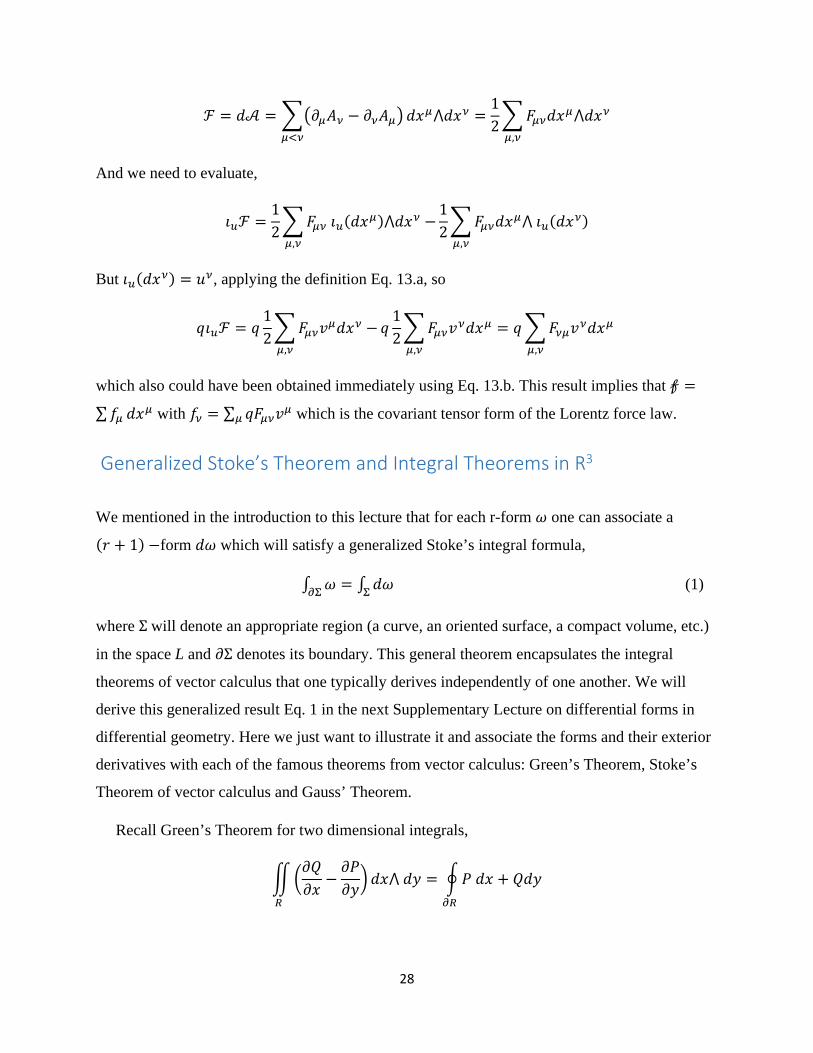
Generalized Stoke’s Theorem and Integral Theorems in R3

We mentioned in the introduction to this lecture that for each r-form 𝜔𝜔 one can associate a

(𝑟𝑟 + 1) −form 𝑑𝑑𝜔𝜔 which will satisfy a generalized Stoke’s integral formula,

∫ 𝜔𝜔 = ∫ 𝑑𝑑𝜔𝜔Σ𝜕𝜕Σ (1)

where Σ will denote an appropriate region (a curve, an oriented surface, a compact volume, etc.)

in the space L and 𝜕𝜕Σ denotes its boundary. This general theorem encapsulates the integral

theorems of vector calculus that one typically derives independently of one another. We will

derive this generalized result Eq. 1 in the next Supplementary Lecture on differential forms in

differential geometry. Here we just want to illustrate it and associate the forms and their exterior

derivatives with each of the famous theorems from vector calculus: Green’s Theorem, Stoke’s

Theorem of vector calculus and Gauss’ Theorem.

Recall Green’s Theorem for two dimensional integrals,

��𝜕𝜕𝑄𝑄𝜕𝜕𝜕𝜕

−𝜕𝜕𝑃𝑃𝜕𝜕𝑑𝑑�

𝑅𝑅

𝑑𝑑𝜕𝜕⋀ 𝑑𝑑𝑑𝑑 = �𝑃𝑃 𝑑𝑑𝜕𝜕 + 𝑄𝑄𝑑𝑑𝑑𝑑𝜕𝜕𝑅𝑅

29

where R is a planar region and 𝜕𝜕𝑅𝑅 is its boundary. If we take 𝜔𝜔 = 𝑃𝑃 𝑑𝑑𝜕𝜕 + 𝑄𝑄𝑑𝑑𝑑𝑑, then we have

calculated in several illustrations above that 𝑑𝑑𝜔𝜔 = �𝜕𝜕𝜕𝜕𝜕𝜕𝑥𝑥− 𝜕𝜕𝜕𝜕

𝜕𝜕𝑦𝑦� 𝑑𝑑𝜕𝜕⋀ 𝑑𝑑𝑑𝑑, and we see that Green’s

Theorem is just a special case of the generalized Stoke’s theorem Eq.1.

Next we have Stoke’s Theorem of vector calculus. Let there be a vector field in R3, 𝑉𝑉�⃗ =

𝑃𝑃𝚤𝚤̂ + 𝑄𝑄𝚥𝚥̂ + 𝑅𝑅𝑘𝑘� and let there be an oriented surface S with boundary curve 𝜕𝜕𝜕𝜕. Then,

��∇��⃗ × 𝑉𝑉�⃗ � ∙ 𝑑𝑑�⃗�𝑎𝑆𝑆

= �𝑉𝑉�⃗ ∙ 𝑑𝑑𝑟𝑟𝜕𝜕𝑆𝑆

This time we define the 1-form 𝜔𝜔 = 𝑃𝑃 𝑑𝑑𝜕𝜕 + 𝑄𝑄𝑑𝑑𝑑𝑑 + 𝑅𝑅 𝑑𝑑𝑑𝑑 and calculate its exterior derivative,

𝑑𝑑𝜔𝜔 = �𝜕𝜕𝑄𝑄𝜕𝜕𝜕𝜕

−𝜕𝜕𝑃𝑃𝜕𝜕𝑑𝑑�

𝑑𝑑𝜕𝜕⋀𝑑𝑑𝑑𝑑 + �𝜕𝜕𝑃𝑃𝜕𝜕𝑑𝑑

−𝜕𝜕𝑅𝑅𝜕𝜕𝜕𝜕�

𝑑𝑑𝑑𝑑⋀𝑑𝑑𝜕𝜕 + �𝜕𝜕𝑅𝑅𝜕𝜕𝑑𝑑

−𝜕𝜕𝑄𝑄𝜕𝜕𝑑𝑑�

𝑑𝑑𝑑𝑑⋀𝑑𝑑𝑑𝑑

Then we see that Stoke’s Theorem of vector calculus is another example of the generalized

Stoke’s Theorem Eq.1. We need only write the surface element vector differential 𝑑𝑑�⃗�𝑎 in

Cartesian coordinates as was done in the introductory section of this lecture.

Finally, we have Gauss’ Theorem. Again, identify a vector field in R3, 𝑉𝑉�⃗ = 𝑃𝑃𝚤𝚤̂ + 𝑄𝑄𝚥𝚥̂ + 𝑅𝑅𝑘𝑘�

and let there be a three dimensional region R with oriented boundary surface 𝜕𝜕𝑅𝑅. Then,

�∇��⃗ ∙ 𝑉𝑉�⃗ 𝑑𝑑𝜕𝜕⋀𝑑𝑑𝑑𝑑⋀𝑑𝑑𝑑𝑑𝑅𝑅

= �𝑉𝑉�⃗ ∙ 𝑑𝑑�⃗�𝑎𝜕𝜕𝑅𝑅

If we define the 2-form 𝜔𝜔 = 𝑃𝑃 𝑑𝑑𝑑𝑑⋀𝑑𝑑𝑑𝑑 + 𝑄𝑄 𝑑𝑑𝑑𝑑⋀𝑑𝑑𝜕𝜕 + 𝑅𝑅 𝑑𝑑𝜕𝜕⋀𝑑𝑑𝑑𝑑, then its exterior derivative is,

𝑑𝑑𝜔𝜔 = �𝜕𝜕𝜕𝜕𝜕𝜕𝑥𝑥

+ 𝜕𝜕𝜕𝜕𝜕𝜕𝑦𝑦

+ 𝜕𝜕𝑅𝑅𝜕𝜕𝑧𝑧

� 𝑑𝑑𝜕𝜕⋀𝑑𝑑𝑑𝑑⋀𝑑𝑑𝑑𝑑, and the generalized Stoke’s Theorem Eq.1 reproduces Gauss’

Law.

All this illustrates how differential forms unify otherwise diverse results in vector calculus.

When we turn to differential geometry and general relativity, we shall find more

challenging examples of this trend.

References

30

1. H. Flanders, Differential Forms with Applications to the Physical Sciences, Academic

Press, New York, 1963.

2. M. P. Do Carmo, Differential Forms and Applications, Springer-Verlag, Berlin, 1971.

3. T. Frankel, The Geometry of Physics. An Introduction, Cambridge University Press,

Cambridge, 1997.