Introduction p;q -tensor Basic notation. n ;:::;x Msvante/papers/sjN15.pdf · elegant in...
122
RIEMANNIAN GEOMETRY: SOME EXAMPLES, INCLUDING MAP PROJECTIONS SVANTE JANSON Abstract. Some standard formulas are collected on curvature in Rie- mannian geometry, using coordinates. (There are, as far as I know, no new results). Many examples are given, in particular for manifolds with constant curvature, including many well-known map projections of the sphere and several well-known representations of hyperbolic space, but also some lesser known. 1. Introduction We collect general formulas on curvature in Riemannian geometry and give some examples, with emphasis on manifolds with constant curvature, in particular some standard map projections of the sphere (Section 6) and some standard representations of hyperbolic space (Section 7). We work with coordinates, and therefore represent tensors as indexed quantities A i 1 ,...,ip j 1 ,...,jq with arbitrary numbers p > 0 and q > 0 of indices (con- travariant and covariant, respectively); we say that this tensor is of type (p, q), or a (p, q)-tensor. Some formulas and calculations are much more elegant in coordinate-free formulations, see e.g. [4], but our emphasis is on explicit calculations. We assume knowledge of basic tensor calculus, including covariant and contravariant tensors, contractions and raising and lowering of indices. 1.1. Basic notation. We consider an n-dimensional Riemannian manifold M and a coordinate system (x 1 ,...,x n ), i.e. a diffeomorphic map of an open subset of M onto an open subset of R n ; we assume n > 2. All indices thus take the values 1,...,n. We use the Einstein summation convention: a i i means ∑ n i=1 a i i . The metric tensor is g ij , and the inverse matrix is denoted g ij : ( g ij ) = ( g ij ) -1 (1.1) or in the usual notation with coordinates g ik g kj = δ i j , (1.2) where δ i j denotes the Kronecker delta. (We may also write δ ij when more convenient, which often is the case when considering an example with a given Date : 1 March, 2015; revised 14 March, 2015. 1
Transcript of Introduction p;q -tensor Basic notation. n ;:::;x Msvante/papers/sjN15.pdf · elegant in...

RIEMANNIAN GEOMETRY: SOME EXAMPLES,
INCLUDING MAP PROJECTIONS
SVANTE JANSON
Abstract. Some standard formulas are collected on curvature in Rie-mannian geometry, using coordinates. (There are, as far as I know, nonew results). Many examples are given, in particular for manifolds withconstant curvature, including many well-known map projections of thesphere and several well-known representations of hyperbolic space, butalso some lesser known.
1. Introduction
We collect general formulas on curvature in Riemannian geometry andgive some examples, with emphasis on manifolds with constant curvature,in particular some standard map projections of the sphere (Section 6) andsome standard representations of hyperbolic space (Section 7).
We work with coordinates, and therefore represent tensors as indexed
quantities Ai1,...,ipj1,...,jq
with arbitrary numbers p > 0 and q > 0 of indices (con-
travariant and covariant, respectively); we say that this tensor is of type(p, q), or a (p, q)-tensor. Some formulas and calculations are much moreelegant in coordinate-free formulations, see e.g. [4], but our emphasis is onexplicit calculations.
We assume knowledge of basic tensor calculus, including covariant andcontravariant tensors, contractions and raising and lowering of indices.
1.1. Basic notation. We consider an n-dimensional Riemannian manifoldM and a coordinate system (x1, . . . , xn), i.e. a diffeomorphic map of an opensubset of M onto an open subset of Rn; we assume n > 2. All indices thustake the values 1, . . . , n. We use the Einstein summation convention: aiimeans
∑ni=1 a
ii.
The metric tensor is gij , and the inverse matrix is denoted gij :(gij)
=(gij)−1
(1.1)
or in the usual notation with coordinates
gikgkj = δij , (1.2)
where δij denotes the Kronecker delta. (We may also write δij when moreconvenient, which often is the case when considering an example with a given
Date: 1 March, 2015; revised 14 March, 2015.
1
2 SVANTE JANSON
coordinate system.) Recall that the metric tensor is symmetric: gij = gjiand note that contracting the metric tensor or δ yields the dimension:
gijgij = δii = n. (1.3)
We denote the determinant of a 2-tensor A = (Aij) by |A|. In particular,
|g| := det(gij). (1.4)
It is easily seen, using (1.2) and expansions of the determinant, that
∂|g|∂gij
= |g|gij . (1.5)
The invariant measure µ on M is given by
dµ = |g|1/2 dx1 · · · dxn. (1.6)
(This measure can be defined in an invariant way as the n-dimensionalHausdorff measure on M .)
The volume scale is thus |g|−1/2.
1.2. Distortion. The condition number κ > 1 of the metric tensor gij (ata given point) is the ratio between the largest and smallest eigenvalue ofgij . Thus κ = 1 if and only if gij is conformal. It is seen, by taking an ONbasis diagonalizing gij , that the map maps infinitesimally small spheres to
ellipsoids with the ratio of largest and smallest axes κ1/2, and conversely,infinitesimally small spheres on the map correspond to ellipsoids with thisratio of largest and smallest axes. We define
ε :=√
1− 1/κ. (1.7)
Thus 0 6 ε < 1, and ε = 0 if and only if gij is conformal. If n = 2, thenε is the eccentricity of the ellipses that correspond to (infinitesimally) smallcircles by either the coordinate map or its inverse.
If n = 2, then the two eigenvalues of the matrix gij are, with τ :=Tr(gij) = g11 + g22,
τ ±√τ2 − 4|g|2
=g11 + g22 ±
√(g11 + g22)2 − 4|g|
2(1.8)
and thus
κ =g11 + g22 +
√(g11 + g22)2 − 4|g|
g11 + g22 −√
(g11 + g22)2 − 4|g|=g11 + g22 +
√(g11 − g22)2 + 4g2
12
g11 + g22 −√
(g11 − g22)2 + 4g212
(1.9)and, by (1.7),
ε2 =2√
(g11 + g22)2 − 4|g|g11 + g22 +
√(g11 + g22)2 − 4|g|
=2√
(g11 − g22)2 + 4g212
g11 + g22 +√
(g11 − g22)2 + 4g212
.
(1.10)
RIEMANNIAN GEOMETRY: SOME EXAMPLES 3
1.3. Derivatives. We denote partial derivatives simply by indices after acomma:
Apq...kl...,i :=∂
∂xiApq...kl... (1.11)
and similarly for higher derivatives.The Levi-Civita connection has the components
Γmij = gmkΓkij (1.12)
whereΓkij = 1
2
(gki,j + gkj,i − gij,k
). (1.13)
(Γkij is often denote [ij, k]. Γkij and Γkij are also called the Christoffel
symbols of the first and second kind.) Note that Γkij is symmetric in i andj:
Γkij = Γkji. (1.14)
(This says that the Levi-Civita connection that is used in a Riemannianmanifold is torsion-free.)
The covariant derivative of a tensor field is denoted by indices after asemicolon. Recall that for a function (scalar) f , the covariant derivativeequals the usual partial derivative in (1.11):
f;i = f,i. (1.15)
For a contravariant vector field Ak we have
Ak;i = Ak,i + ΓkjiAj (1.16)
and for a covariant vector field Ak we have
Ak;i = Ak,i − ΓjkiAj (1.17)
and for tensor fields of higher order we similarly add to the partial derivativeone term as in (1.16) for each contravariant index and subtract one term asin (1.17) for each covariant index, for example
Aijkl;m = Aijkl,m + ΓipmApjkl − ΓpjmA
ipkl − ΓpkmA
ijpl − ΓplmA
ijkp. (1.18)
Recall that the Levi-Civita connection has the property that the covariantderivative of the metric tensor vanishes:
gij;k = 0; (1.19)
indeed, this together with (1.14) is easily seen to be equivalent to (1.13).Higher covariant derivatives are defined by iteration, for example
f;ij := (f;i);j = f,ij − Γkijf,k. (1.20)
Recall that the covariant derivative of a tensor field is a tensor field, i.e.,invariant in the right way under changes of coordinates, while the partialderivative is not (except for a scalar field, where the two derivatives are thesame, see (1.15)).
A simple calculation, using integration by parts in coordinate neighbour-hoods together with (1.6), (1.5), (1.16) and (1.19), shows that if f is a

4 SVANTE JANSON
smooth function and Ai is a vector field, and at least one of them has com-pact support, then ∫
Mf,iA
i dµ = −∫MfAi;i dµ. (1.21)
If Aij and Bij are symmetric covariant 2-tensors, we define their Kulkarni–Nomizu product to be the covariant 4-tensor
Aij Bkl := AikBjl +AjlBik −AilBjk −AjkBil. (1.22)
We may also use the notation (AB)ijkl. (The notation AijBkl is slightlyimproper, but will be convenient. The notation (A B)ijkl is formallybetter.) Note that AB = B A.
Remark 1.1. The Kulkarni–Nomizu product in (1.22) is the bilinear ex-tension of the map
(AiCj , BkDl) 7→ AiCj BkDl = (Ai ∧Bj)(Ck ∧Dl) (1.23)
where Ai ∧Bj := AiBj −AjBi is the exterior product.
1.4. The Laplace–Beltrami operator. The Laplace–Beltrami operator∆ is a second-order differential operator defined on (smooth) functions onM as the contraction of the second covariant derivative:
∆F := gijF;ij = gijF,ij − gijΓkijF,k. (1.24)
A function F is harmonic if ∆F = 0.For an extension to differential forms, see e.g. [19, Chapter 6].The integration by parts formula (1.21) implies that if F andG are smooth
functions and at least one of them has compact support, then∫MF∆Gdµ = −
∫MgijF,iG,j dµ =
∫MG∆F dµ. (1.25)
In particular, if M is compact, then this holds for all smooth F and G andshows that −∆ is a non-negative operator. (For this reason, the Laplace–Beltrami operator is sometimes defined with the opposite sign.) See further[19].
1.5. Curves. Let γ : (a, b)→ M be a smooth curve, i.e., a smooth map ofan open interval into the Riemannian manifold M . Let Dt denote covariantdifferentiation along γ. For a tensor field Apq...kl... it can be defined by
DtApq...kl... (γ(t)) = Apq...kl...;i(γ(t))γi(t); (1.26)
for example, for a tensor of type (1,1), cf. (1.16)–(1.18),
DtApk(γ(t)) =
(Apk,i + ΓpjiA
jk − ΓjkiA
pj
)γi(t)
=d
dtApk(γ(t)) + ΓpjiA
jkγ
i − ΓjkiApj γi. (1.27)
However, this depends only on the values of the tensor field along the curve,and thus it can be defined for any tensor Apq...kl... (t) defined along the curve.
RIEMANNIAN GEOMETRY: SOME EXAMPLES 5
For each t ∈ (a, b), Dtγ(t) = γ(t) is the tangent vector at γ(t) withcomponents γi(t) = d
dtγi(t); this is called the velocity vector, and the velocity
is its length
‖γ‖ := 〈γ, γ〉1/2 =(gij γ
iγj)1/2
. (1.28)
The acceleration is the vector D2t γ(t) which has components, cf. (1.26)–
(1.27),
D2t γ
i = Dtγi = γi + Γijkγ
j γk, (1.29)
where Γijk = Γijk(γ).Since the covariate derivative Dg = 0 for the Levi-Civita connection, see
(1.19),
Dt
(gij γ
iγj)
= gijDtγiγj + gij γ
iDtγj = 2〈Dtγ, γ〉 = 2〈D2
t γ, γ〉. (1.30)
Consequently, γ has constant velocity, i.e., 〈γ, γ〉 = gij γiγj is constant, if
and only if the acceleration is orthogonal to the velocity vector.Let, assuming γ 6= 0,
PND2t γ := D2
t γ −〈D2
t γ, γ〉〈γ, γ〉
γ (1.31)
be the normal component of the acceleration, i.e., the component orthogonalto the velocity. The (geodesic) curvature κ of the curve is
κ = κ(t) = ‖PND2t γ‖/‖Dtγ‖2; (1.32)
this is invariant under reparametrization of γ (including time-reversal). Wethus may assume that γ is parametrized by arc length, i.e., ‖Dtγ‖ = 1. Inthis case, the acceleration and velocity vectors are orthogonal as said above,so PND
2t γ = D2
t γ and thus
κ = ‖D2t γ‖ if ‖γ‖ = 1. (1.33)
We usually consider the curvature as the non-negative number κ, but wecan also give it a direction and consider the curvature vector, which is thetangent vector
~κ := PND2t γ/‖Dtγ‖2; (1.34)
this too is invariant under reparametrization (including time-reversal). Notethat
‖~κ‖ = κ (1.35)
and that (by definition) ~κ is orthogonal to the velocity vector γ.
Remark 1.2. In an oriented 2-dimensional manifold, we can alternativelyconsider the curvature κ with sign, with κ > 0 if ~κ is to the left of γ. (Notethat the sign changes under time-reversal.) See further Appendix C forcurves in the complex plane.
6 SVANTE JANSON
1.6. Geodesics. A geodesic is a curve γ(t) with acceleration D2t γ = 0, i.e.,
by (1.29), a curve γ(t) such that
γi + Γijk(γ)γj γk = 0. (1.36)
By (1.30), a geodesic has constant velocity.If the connection has the special form
Γkij = δki aj + δkj ai (1.37)
for some functions ai, then (1.36) becomes
γi = −2aj(γ)γj γi (1.38)
which shows that γ is parallel to γ; consequently each geodesic is a straightline in the coordinates xi. The converse holds too, so straight lines aregeodesics if and only if the connection is of the form (1.37), see Theorem D.1.
2. The curvature tensors
2.1. The Riemann curvature tensor. Covariant differentiation is notcommutative. For a contravariant vector field Ai we have
Ai;jk −Ai;kj = RilkjAl, (2.1)
where the tensor Rilkj , the Riemann curvature tensor, is given by
Rijkl = Γijl,k − Γijk,l + ΓiksΓsjl − ΓilsΓ
sjk. (2.2)
The covariant form Rijkl = gimRmjkl of the curvature tensor is given by
Rijkl = 12
(gil,jk + gjk,il − gik,jl − gjl,ik
)+ gpq
(ΓpilΓ
qjk − ΓpikΓ
qjl
). (2.3)
For a covariant vector field Ai we have the analoguous commutation re-lation
Ai;jk −Ai;kj = −RlikjAl, (2.4)
and similarly for tensors of higher order (with one term for each index).
Remark 2.1. In (2.1) and (2.4), it might seem more natural to reverse theorder of the last two indices in the curvature tensor, which means replacingRijkl in (2.2) by Rijlk = −Rijkl. This convention also occurs in the literature,
but the one used here seems to be more common. (The difference is thusin the sign of Rijkl. The Ricci tensor Rij defined below is defined to be the
same in any case.)
Note the symmetries
Rijkl = −Rijlk = −Rjikl = Rjilk (2.5)
and
Rijkl = Rklij . (2.6)
In particular, with two coinciding indices,
Riikl = Rijkk = 0. (2.7)

RIEMANNIAN GEOMETRY: SOME EXAMPLES 7
Moreover, (2.3) also implies the Bianchi identity
Rijkl +Riklj +Riljk = 0. (2.8)
Note also the second Bianchi identity
Rijkl;m +Rijlm;k +Rijmk;l = 0. (2.9)
Four distinct indices i, j, k, l can be permuted in 24 ways, and (2.5)–(2.6)show that only three of the resulting Rijkl are essentially distinct; each ofthe 24 equals ±Rijkl, ±Riklj or ±Riljk. Moreover, two of these three valuesdetermine the third by the Bianchi identity. Hence, of these 24 differentvalues, there are only 2 linearly independent. See further Appendix A.
2.2. The Ricci tensor. The Ricci tensor is defined as the contraction
Rij := Rkikj = gklRkilj = gklRikjl
= Γkij,k − Γkik,j + ΓkksΓsij − ΓkjsΓ
sik. (2.10)
The Ricci tensor is symmetric,
Rij = Rji, (2.11)
as a consequence of (2.6).The second Bianchi identity (2.9) implies
Rijkl;i = gimRijkl;m = Rjl;k −Rjk;l. (2.12)
2.3. Scalar curvature. The scalar curvature is the contraction (trace) ofthe Ricci tensor
R := Rii = gijRij = gijgklRikjl. (2.13)
The second Bianchi identity (2.9), or (2.12), implies
R,i = R;i = 2Rki;k = 2gjkRij;k. (2.14)
2.4. The Weyl tensor. When n > 3, the curvature tensor can be decom-posed as
Rijkl =1
2n(n− 1)Rgij gkl +
1
n− 2
(Rij −
1
nRgij
) gkl +Wijkl, (2.15)
where
Wijkl := Rijkl −1
n− 2Rij gkl +
1
2(n− 1)(n− 2)Rgij gkl (2.16)
is the Weyl tensor. The two first terms on the right-hand side of (2.15) canbe seen as the parts of Rijkl determined by the scalar curvature R and the
traceless part of the Ricci curvature Rij − 1nRgij ; together they thus yield
the part of Rijkl determined by the Ricci tensor, and the Weyl tensor is theremainder; see Appendix A.
The Weyl tensor satisfies the same symmetry relations (2.5)–(2.6) and(2.8) as the Riemann curvature tensor, see Appendix A. Furthermore, thecontraction vanishes:
W kikj = gklWkilj = gklWikjl = 0, (2.17)
8 SVANTE JANSON
see (A.20)–(A.23).When n = 2, the Weyl tensor is trivially defined to be 0. Moreover, then
Rij − 1nRgij = 0, and (2.15) still holds in the form
Rijkl =1
2n(n− 1)Rgij gkl +Wijkl =
1
4Rgij gkl, (2.18)
see (A.28).Also when n = 3, the Weyl tensor Wijkl vanishes identically; (2.15) then
becomes, see (A.27),
Rijkl =1
12Rgij gkl +
(Rij −
1
3Rgij
) gkl =
(Rij −
1
4Rgij
) gkl.
(2.19)
2.5. The traceless Ricci tensor. The traceless Ricci tensor is defined as
Tij := Rij −1
nRgij ; (2.20)
thus the contractionT ii := gijTij = 0, (2.21)
which explains its name. Note that Tij = 0 if and only if Rij is a multiple
of gij . See further Appendix A; Tij is the traceless component denoted R(2)ij
in (A.8) and (A.10).
2.6. The Schouten tensor. The Schouten tensor is the symmetric tensordefined, for n > 3, by
Sij :=1
n− 2Rij−
R
2(n− 1)(n− 2)gij =
1
n− 2
(Rij−
1
2(n− 1)Rgij
); (2.22)
thus (2.16) can be written as
Wijkl = Rijkl − Sij gkl. (2.23)
Equivalently,Rijkl = Wijkl + Sij gkl, (2.24)
and by (A.15), this is the unique decomposition of Rijkl of this type withtensors Wijkl and Sij such that W i
jil = 0 and Sij = Sji.The contraction is
Sii =1
2(n− 1)R. (2.25)
2.7. The Einstein tensor. The Einstein tensor is defined as
Gij = Rij − 12Rgij = Rij − 1
2gijgklRkl (2.26)
or equivalentlyGij = Rij − 1
2Rgij . (2.27)
The Einstein tensor Gij is symmetric, and it follows from (2.14) that itsdivergence vanishes:
Gij ;j = 0. (2.28)
RIEMANNIAN GEOMETRY: SOME EXAMPLES 9
The contraction is
Gii = −n− 2
2R. (2.29)
Note that for n > 3, the traceless Ricci tensor (2.20), the Schouten tensor(2.22) and the Einstein tensor (2.26) are three different linear combinationsof Rij and R. (If n = 2, then Gij = Tij and Sij is not defined.)
2.8. The Cotton tensor. The Cotton tensor is defined, for n > 3, as
Cijk := Sij;k − Sik;j . (2.30)
The reason for this definition is that by a simple calculation using (2.16),(2.12) and (2.14),
(n− 2)W ijkl;i := (n− 2)gimWijkl;m
= (n− 2)Rijkl;i−(Rik;igjl−Ril;igjk +Rjl;k −Rjk;l
)+
1
n− 1
(R;kgjl−R;lgjk
)= (n− 3)
(Rjl;k −Rjk;l
)− n− 3
2(n− 1)
(R;kgjl −R;lgjk
)(2.31)
and thus
W ijkl;i = (n− 3)
(Sjl;k − Sjk;l
)= −(n− 3)Cjkl. (2.32)
2.9. Sectional curvature. Let σ be a two-dimensional subspace of thetangent space Mx at some point x, and let U and V be two tangent vectorsspanning σ (i.e., any two linearly independent vectors in σ). Then thesectional curvature at σ is defined as
K(σ) := K(U, V ) :=RijklU
iV jUkV l
‖U ∧ V ‖2(2.33)
where we define the norm of the 2-form U ∧ V = U iV j − U jV i by
‖U ∧ V ‖2 := 12gikgjl(U
iV j − U jV i)(UkV l − U lV k)
= 12(gij gkl)U iV jUkV l
= 〈U,U〉〈V, V 〉 − 〈U, V 〉2. (2.34)
It is easily seen that the fractions in (2.33) are the same for any pair of vectorsU and V spanning σ; thus K(U, V ) depends only on σ which justifies thedefinition of K(σ). By (2.34) we can also write
K(σ) := K(U, V ) =RijklU
iV jUkV l
12(gij gkl)U iV jUkV l
. (2.35)
A Riemannian manifold M is isotropic if K(σ) = K(x) is the same forall two-dimensional subspaces σ of Mx, for every x ∈M . This is equivalentto, see [4, Lemmas 3.3 and 3.4],
Rijkl = K(x)12 gij gkl = K(x)
(gikgjl − gilgjk
). (2.36)
10 SVANTE JANSON
By (2.15) (and (2.18) when n = 2), see further Appendix A, this is alsoequivalent to
Wijkl = 0 and Rij = 1nRgij . (2.37)
For an isotropic manifold we have, with K = K(x), as a consequence of(2.36),
Rij = (n− 1)Kgij , (2.38)
R = n(n− 1)K. (2.39)
Moreover, by (2.20), (2.22) and (2.26),
Tij = 0, (2.40)
Sij = 12Kgij (n > 3), (2.41)
Gij = −(n− 1)(n− 2)
2Kgij . (2.42)
A Riemannian manifold M is of constant (sectional) curvature if K(σ) =K is the same for all two-dimensional subspaces σ ofMx for all points x ∈M ,i.e., if M is isotropic and K(x) is a constant function. In other words, by(2.36), M is of constant curvature if and only if
Rijkl = 12K gij gkl = K
(gikgjl − gilgjk
)(2.43)
for some constant K; in this case (2.38)–(2.39) hold, and in particular K =R/(n(n− 1)).
Every two-dimensional manifold is isotropic by definition, or by (2.18),but not necessarily of constant curvature.
On the other hand, if M is isotropic then Rij = 1nRgij so (2.14) yields
R;i = 2gjkRij;k = 2ng
jkR;k gij = 2nR;i. (2.44)
Hence, if furthermore n > 3, then R,i = R;i = 0 and thus R is locallyconstant. Thus a connected manifold with dimension > 3 is isotropic if andonly if it is of constant curvature. (In other words, a connected manifold isisotropic if and only if it has dimension 2 or has constant curvature.)
It follows from (2.30) and (2.41) that for a manifold with constant curva-ture and n > 3, Cijk = 0. Furthermore, Wijkl = 0 by (2.37).
3. Special cases
3.1. The two-dimensional case. If n = 2, the only non-zero componentsof Rijkl are, by (2.5)–(2.6),
R1212 = R2121 = −R1221 = −R2112. (3.1)
It follows from (2.10) that, with R := R1212,
R11 = Rg22, R22 = Rg11, R12 = R21 = −Rg12 (3.2)
and thus by (1.1)
Rij = R|g|−1gij (3.3)

RIEMANNIAN GEOMETRY: SOME EXAMPLES 11
and
R = 2|g|−1R. (3.4)
This can also be written
R1212 = R2121 = −R1221 = −R2112 = 12 |g|R (3.5)
or, equivalently,
Rijkl = 12R(gikgjl − gilgjk
)= 1
4Rgij gkl, (3.6)
and
Rij = 12Rgij . (3.7)
(See (A.28)–(A.29) for alternative proofs.)By (3.6) and (2.36), the metric is isotropic with sectional curvature
K = 12R. (3.8)
The Weyl tensor vanishes by definition: Wijkl = 0.Also the Einstein tensor vanishes: Gij = 0 by (3.7) and (2.26).The Schouten and Cotton tensors are not defined.For the special case of a smooth surface in R3, the Gaussian curvature
at a point p can be defined as the product of the two principal curvaturesat p (or as the determinant of the shape operator S : Mp → Mp given by
S(v) = − ∂∂vN , where N is the unit normal field). The Gaussian curvature
equals the sectional curvature K.
3.2. Flat metric. A Riemannian manifold M is flat if it locally is isometricto Euclidean space, i.e., if it can be covered by coordinate systems withgij = δij . It follows immediately by (1.13) and (1.12) that the connection
coefficients Γkij and Γkij vanish; hence by (2.2), the curvature tensor vanishes:
Rijkl = 0. Conversely, it is well-known that the converse also holds (see e.g.[4, Corollary 8.2.2]):
Theorem 3.1. A manifold M is flat if and only if Rijkl = 0.
By (2.43), M is flat if and only if it is of constant curvature 0.It follows immediately from the definitions above that in a flat manifold,
also the Ricci tensor, Weyl tensor, Einstein tensor and scalar curvaturevanish, as well as, when n > 3, the Schouten and Cotton tensors. Conversely,we see for example from (2.15) (and (2.18) when n = 2) that M is flat if andonly if the Weyl and Ricci tensors vanish; in particular, if n = 3 then M isflat if and only if the Ricci tensor vanishes. Similarly, by (2.24), if n > 3,then M is flat if and only if the Weyl and Schouten tensors vanish.
3.3. Conformal metric. Consider a conformal Riemannian metric
ds = w(x)|dx| = eϕ(x)|dx|. (3.9)
In other words,
gij = w(x)2δij = e2ϕ(x)δij . (3.10)

12 SVANTE JANSON
Thengij = w(x)−2δij = e−2ϕ(x)δij . (3.11)
The invariant measure (1.6) is
dµ = w(x)n dx1 · · · dxn = enϕ(x) dx1 · · · dxn. (3.12)
We have, cf. [4, Section 8.3],
Γkij = [ij, k] = ww,iδjk + ww,jδik − ww,kδij . (3.13)
and thusΓkij = ϕ,iδjk + ϕ,jδik − ϕ,kδij . (3.14)
It follows by a calculation that, with ‖∇ϕ‖2 =∑n
i=1 ϕ2,i,
Rijkl = e2ϕ(
(ϕ,iϕ,j − ϕ,ij) δkl − ‖∇ϕ‖2(δikδjl − δilδjk))
= e2ϕ(ϕ,iϕ,j − ϕ,ij − 1
2‖∇ϕ‖2δij
) δkl, (3.15)
and thus, by another calculation, with ∆ϕ :=∑n
i=1 ϕ,ii,
Rij = (n− 2)(ϕ,iϕ,j − ϕ,ij − ‖∇ϕ‖2δij
)−∆ϕ δij (3.16)
and
R = −e−2ϕ(
(n− 1)(n− 2)‖∇ϕ‖2 + 2(n− 1)∆ϕ). (3.17)
The Weyl tensor thus vanishes, by (2.16), or by (A.20),
Wijkl = 0. (3.18)
The Einstein tensor is
Gij = (n− 2)(ϕ,iϕ,j − ϕ,ij + 1
2(n− 3)‖∇ϕ‖2δij + ∆ϕ δij
). (3.19)
For n > 3, the Schouten tensor is by (3.15)
Sij = ϕ,iϕ,j − ϕ;ij − 12‖∇ϕ‖
2gij (3.20)
and a calculation shows that the Cotton tensor vanishes:
Cijk = 0. (3.21)
The Laplace–Beltrami operator ∆ is given by
∆F = e−2ϕ
(n∑i=1
F,ii + (n− 2)
n∑i=1
ϕ,iF,i
)(3.22)
= w−nn∑i=1
(wn−2F,i),i. (3.23)
A Riemannian manifold M is (locally) conformally flat if it locally isconformally equivalent to Euclidean space, i.e., if it can be covered by co-ordinate systems with metrics as in (3.10). (Such coordinates are calledisothermal.) A manifold of dimension 2 is always conformally flat. (By The-orem 3.1, (3.6) and (3.43) below, this is equivalent to the existence of localsolutions to ∆ϕ = R/2. See e.g. [6, P.4.8] together with [19, Theorem 6.8]
RIEMANNIAN GEOMETRY: SOME EXAMPLES 13
for a proof. This holds also under much weaker regularity, see e.g. Korn [9],Lichtenstein [12], Chern [2] and Hartman and Wintner [5].) If n > 3, (3.18)and (3.21) show that if M is conformally flat, then Wijkl = 0 and Cijk = 0.The Weyl–Schouten theorem says that the converse holds too; moreover, ifn = 3 then Wijkl = 0 automatically, and if n > 4, then Wijkl = 0 in Mimplies Cijk = 0 by (2.32). Hence we have the following characterisation.(For a proof, see e.g. [6]. The necessity of Wijkl = 0 when n > 4 was shownby Weyl [18] and the sufficiency by Schouten [14]; the case n = 3 was treatedearlier by Cotton [3].)
Theorem 3.2 (Weyl–Schouten). M is conformally flat if and only if
• n = 2,• n = 3 and Cijk = 0, or• n > 4 and Wijkl = 0.
Note that for n = 3 the condition is a third-order system of partial dif-ferential equations in gij , but for n > 4 only a second-order system.
3.3.1. The case n = 2. For a conformal Riemannian metric in the specialcase n = 2, when (3.6)–(3.7) hold, (3.15)–(3.17) simplify to
Rijkl = −12e
2ϕ∆ϕ δij δkl, (3.24)
Rij = −∆ϕ δij , (3.25)
R = −2e−2ϕ∆ϕ. (3.26)
The sectional curvature is, by (2.36) or (3.8),
K = R/2 = −e−2ϕ∆ϕ. (3.27)
The Laplace–Beltrami operator is by (3.22)
∆F = e−2ϕn∑i=1
F,ii. (3.28)
In particular, the coordinate functions xj are harmonic, since xj,ii = 0.
3.4. Conformally equivalent metrics. More generally, consider two con-formally equivalent Riemannian metrics gij and
gij = w(x)2gij = e2ϕ(x)gij . (3.29)
We denote quantities related to gij by a tilde. Note that covariant derivativesand norms below are calculated for gij .
We have
gij = w(x)−2gij = e−2ϕ(x)gij . (3.30)
Calculations show that
Γkij = Γkij + ϕ,iδkj + ϕ,jδ
ki − gklϕ,l gij (3.31)

14 SVANTE JANSON
and, with ‖∇ϕ‖2 := gijϕ,iϕ,j and ∆ϕ := gijϕ;ij as in (1.24),
Rijkl = e2ϕ(Rijkl + (ϕ,iϕ,j − ϕ;ij) gkl − 1
2‖∇ϕ‖2gij gkl
)= e2ϕ
(Rijkl +
(ϕ,iϕ,j − ϕ;ij − 1
2‖∇ϕ‖2gij) gkl
), (3.32)
Rij = Rij + (n− 2)(ϕ,iϕ,j − ϕ;ij − ‖∇ϕ‖2gij
)−∆ϕgij , (3.33)
R = e−2ϕ(R− (n− 1)(n− 2)‖∇ϕ‖2 − 2(n− 1)∆ϕ
); (3.34)
for n > 2, the latter formula can also be written
R = e−2ϕ(R− 4(n− 1)
n− 2e−(n−2)ϕ/2∆e(n−2)ϕ/2
). (3.35)
The Weyl tensor is, by (2.16), or by (A.20),
Wijkl = e2ϕWijkl. (3.36)
This becomes nicer for the (3, 1)-tensor W ijkl which is completely invariant:
W ijkl = W i
jkl. (3.37)
The Weyl tensor W ijkl is thus sometimes called the conformal curvature
tensor.The Schouten tensor (for n > 3) transforms as, e.g. by (3.32) and (2.24),
Sij = Sij + ϕ,iϕ,j − ϕ;ij − 12‖∇ϕ‖
2gij . (3.38)
A calculation shows that the Cotton tensor (for n > 3) transforms as
Cijk = Cijk +W lijkϕ,l. (3.39)
In particular, if n = 3, then the Weyl tensor vanishes and Cijk = Cijk, i.e.,the Cotton tensor is conformally invariant.
The Laplace–Beltrami operator ∆ transforms as
∆F = e−2ϕ(∆F + (n− 2)gijϕ,iF,j
). (3.40)
3.4.1. The case n = 2. In the special case n = 2, when (3.6)–(3.7) hold,(3.32)–(3.34) simplify to
Rijkl = e2ϕ(Rijkl − 1
2∆ϕgij gkl)
(3.41)
Rij = Rij −∆ϕgij , (3.42)
R = e−2ϕ(R− 2∆ϕ
). (3.43)

RIEMANNIAN GEOMETRY: SOME EXAMPLES 15
3.5. Scaling. As a special case of (3.29), consider scaling all lengths by aconstant factor a > 0:
gij = a2gij . (3.44)
This is (3.29) with w(x) = a and ϕ(x) = log a constant, and thus all deriva-tives ϕ,i = 0.
It follows from (3.30)–(3.39) that
gij = a−2gij , (3.45)
Γkij = Γkij , (3.46)
Rijkl = a2Rijkl, (3.47)
Rij = Rij , (3.48)
R = a−2R, (3.49)
Wijkl = a2Wijkl, (3.50)
Sij = Sij (n > 3), (3.51)
Cijk = Cijk (n > 3). (3.52)
In particular, it follows from (2.43) that if gij has constant curvature K,then gij has constant curvature a−2K.
4. Examples, general
Example 4.1. Let, for x in a suitable domain in Rn,
ds =a |dx|
1 + c|x|2, (4.1)
i.e.,
gij =a2
(1 + c|x|2)2δij . (4.2)
We assume a > 0 and c ∈ R; if c > 0 the metric is defined in Rn, but ifc < 0 only for |x| < |c|−1/2. (It is also possible to take a < 0, c < 0 and
|x| > |c|−1/2. The results below hold in this case too; see Remark 4.4.)This is a conformal metric (3.10) with w(x) = a/(1 + c|x|2) and ϕ(x) =
log a− log(1 + c|x|2). The invariant measure (1.6) is
dµ = w(x)n dx1 · · · dxn =an
(1 + c|x|2)ndx1 · · · dxn. (4.3)
We have
gij =(1 + c|x|2)2
a2δij (4.4)
and
ϕ,i = − 2cxi1 + c|x|2
(4.5)

16 SVANTE JANSON
and thus by (3.14)
Γkij = − 2c
1 + c|x|2(xiδjk + xjδik − xkδij
). (4.6)
Furthermore,
ϕ,ij = − 2cδij1 + c|x|2
+4c2xixj
(1 + c|x|2)2= − 2c
1 + c|x|2δij + ϕ,iϕ,j , (4.7)
‖∇ϕ‖2 =4c2|x|2
(1 + c|x|2)2, (4.8)
and (3.15) yields
Rijkl =a2
(1 + c|x|2)2
(2c
1 + c|x|2− 2c2|x|2
(1 + c|x|2)2
)δij δkl
=2ca2
(1 + c|x|2)4δij δkl = 2ca−2gij gkl. (4.9)
The metric thus has constant curvature, see (2.43), which also shows thatthe sectional curvature is
K = 4ca−2, (4.10)
and hence, by (2.38)–(2.39), or by (3.16)–(3.17),
Rij = 4(n− 1)ca−2gij =4(n− 1)c
(1 + c|x|2)2δij , (4.11)
R = 4n(n− 1)ca−2. (4.12)
See further Examples 6.1 and 7.3–7.4.
Remark 4.2. Of course, different values of a > 0 in Example 4.1 differ onlyby a simple scaling of the metric, see Section 3.5.
Remark 4.3. Denote the metric (4.2) by g(a,c)ij . If t > 0, then the dilation
ψ(x) = tx maps the metric g(a,c)ij to t−2a2(1 + ct−2|x|2)−2δij , i.e. g
(t−1a,t−2c)ij .
Note that these metrics have the same sectional curvature 4ca−2 by (4.10)(as they must when there is an isometry).
Hence, if c 6= 0, we may by choosing t = |c|1/2 obtain an isometry with
g(a1,c/|c|)ij for some a1, i.e., we may by a dilation assume that c ∈ 0,±1.
The case c = 0 is flat and yields a multiple of the standard Euclideanmetric (a special case of Example 5.1).
The case c = 1 yields a positive curvature K = 4a−2. (This is by adilation x 7→ (a/2)x equivalent to Example 6.1 with ρ = a/2.)
The case c = −1 yields a negative curvature K = −4a−2. (This is Exam-ple 7.4.)
RIEMANNIAN GEOMETRY: SOME EXAMPLES 17
Remark 4.4. As said in Example 4.1, it is possible to take a < 0 in (4.1)–
(4.2) if c < 0 and |x| > |c|−1/2; we thus have
ds =|a||dx||c||x|2 − 1
. (4.13)
The map x 7→ |c|−1x/|x|2, i.e., reflection in the sphere |x| = |c|−1/2, maps
this to the metric g(|a|,c)ij (y) = a2(1 + c|y|2)−2δij in 0 < |y| < |c|−1/2, so this
case is by an isometry equivalent to the case a > 0, c < 0 (with the point 0removed).
Similarly, if c > 0, then the map x 7→ c−1x/|x|2, i.e., reflection in the
sphere |x| = c−1/2, maps the metric (4.1)–(4.2) to itself, so it is an isometry
of Rn \ 0 with the metric g(a,c)ij onto itself.
Example 4.5 (Polar coordinates, general). Let n = 2 and let M be a subsetof R2 = (r, θ) with the metric
|ds|2 = |dr|2 + w(r)2|dθ|2 (4.14)
for some smooth function w(r) > 0, i.e.,
g11 = 1, g12 = g21 = 0, g22 = w(r)2, (4.15)
or in matrix form
(gij) =
(1 00 w(r)2
). (4.16)
(We thus denote the coordinates by r = x1 and θ = x2.)We have
(gij) =
(1 00 w(r)−2
), (4.17)
i.e.,
g11 = 1, g12 = g21 = 0, g22 = w(r)−2. (4.18)
The invariant measure is
dµ = w(r) dr dθ. (4.19)
The only non-zero derivatives gij,k and gij,kl are g22,1 = 2ww′ and g22,11 =2ww′′ + 2(w′)2, with w = w(r), and it follows from (1.13) that
Γ122 = −ww′, (4.20)
Γ212 = Γ221 = ww′, (4.21)
with the remaining components 0, which by (1.12) yields
Γ122 = −ww′, (4.22)
Γ212 = Γ2
21 = w′/w, (4.23)
again with all other components 0.By (2.3), this yields
R1212 = −(ww′′ + (w′)2) + w2(w′/w)2 = −ww′′, (4.24)
18 SVANTE JANSON
and thus, e.g. by (3.3)–(3.4) and (3.8)
Rij = −w′′
wgij , (4.25)
R = −2w′′
w(4.26)
K = −w′′
w. (4.27)
See also the generalization Example 4.6.It is obvious, by translation invariance, that the lines with r constant have
constant curvature. More precisely, if γ(t) = (r, t) for some fixed r, thenγ = (0, 1) and γ = (0, 0), and thus by (1.29)
D2t γ
i = Γijkγj γk = Γi22, (4.28)
i.e., by (4.22) and Γ222 = 0,
D2t γ = (Γ1
22,Γ222) =
(−w(r)w′(r), 0
). (4.29)
Hence, by (1.31),
PND2t γ = D2
t γ =(−w(r)w′(r), 0
). (4.30)
Consequently, the curvature vector (1.34) of γ is
~κ = −(w(r)w′(r), 0
)w(r)2
=(−w
′(r)
w(r), 0)
(4.31)
and the curvature is
κ =|w′(r)|w(r)
. (4.32)
It follows easily from (4.27) that the cases of a metric (4.14)–(4.16) withconstant curvature are, up to translation and reflection in r and dilation inθ, and with some constant a > 0:
(i) w(r) = a (K = 0), see Example 5.1;(ii) w(r) = r (K = 0), see Example 5.2;(iii) w(r) = sin(ar) (K = a2), see Examples 6.7–6.9;(iv) w(r) = ear (K = −a2), see Example 7.2;(v) w(r) = sinh(ar) (K = −a2), see Example 7.8;(vi) w(r) = cosh(ar) (K = −a2), see Example 7.15.
Example 4.6 (Spherical coordinates, general). Example 4.5 can be gener-
alized to arbitrary dimension as follows. Let M be an (n − 1)-dimensional
Riemannian manifold and let M be J × M for an open interval J ⊆ R, withthe metric
|ds|2 = |dr|2 + w(r)2|ds|2, (4.33)
where |ds| is the distance in M . We introduce coordinates x = (x1, . . . , xn−1)
in (a subset of) M and use the coordinates (r, x) = (x0, . . . , xn−1) (with anunusual numbering) in M ; we thus have r = x0. We use α, β, γ, δ to denoteindices in 1, . . . , n− 1.

RIEMANNIAN GEOMETRY: SOME EXAMPLES 19
Denote the metric tensor in M by gαβ; then the metric tensor in M isgiven by
g00 = 1, gαβ = w(x0)2gαβ(x), g0α = gα0 = 0, (4.34)
or in block matrix form(gij)
=
(1 00 w(x0)2gαβ(x)
). (4.35)
It follows from (1.13) that, with w = w(x0) and gαβ = gαβ(x),
Γ000 = Γ00α = Γ0α0 = Γα00 = 0, (4.36)
Γαβ0 = Γα0β = ww′gαβ, (4.37)
Γ0αβ = −ww′gαβ, (4.38)
Γαβγ = w2Γαβγ (4.39)
and thus by (1.12),
Γ000 = Γ0
0α = Γ0α0 = Γα00 = 0, (4.40)
Γαβ0 = Γα0β =w′
wδαβ , (4.41)
Γ0αβ = −ww′gαβ = −w
′
wgαβ, (4.42)
Γαβγ = Γαβγ . (4.43)
This and (2.3) yield
Rαβγδ = w2Rαβγδ + g00
(Γ0αδΓ
0βγ − Γ0
αγΓ0βδ
)= w2Rαβγδ − (w′/w)2
(gαγgβδ − gαδgβγ
), (4.44)
Rαβγ0 = 12
(gβγ,α0 − gαγ,β0
)+ gpq
w′
w
(δpαΓqβγ − δ
qβΓpαγ
)= ww′
(gβγ,α − gαγ,β
)+ ww′
(Γαβγ − Γβαγ
)= 0, (4.45)
Rα0γ0 = −12gαγ,00 + gpq
(w′w
)2δpαδ
qγ = −
(ww′′ + (w′)2
)gαγ + (w′)2gαγ
= −w′′
wgαγ = −w
′′
w
(gαγg00 − gα0g0γ
), (4.46)
Rα000 = R0000 = 0. (4.47)
(The remaining components are given by the symmetry rules (2.5)–(2.6).)By contraction, this further yields the Ricci tensor, see (2.10),
Rαγ = Rαγ +Rα0γ0 −(w′w
)2(n− 2)gαγ
= Rαγ −(
(n− 2)(w′w
)2+w′′
w
)gαγ , (4.48)
Rα0 = 0, (4.49)

20 SVANTE JANSON
R00 = gαγRα0γ0 = −(n− 1)w′′
w(4.50)
and the scalar curvature, see (2.13),
R = w−2(R− (n− 1)(n− 2)(w′)2 − 2(n− 1)ww′′
). (4.51)
The Weyl tensor (2.16) vanishes if n 6 3, as always; for n > 4,
Wαβγδ = w2Wαβγδ +w2
(n− 2)(n− 3)
(Rαβ −
R
n− 1gαβ
) gγδ, (4.52)
Wα0γ0 = − 1
n− 2
(Rαγ −
R
n− 1gαγ
); (4.53)
the remaining components follow by symmetry or vanish.
Now specialize to the case when M has constant curvature, Rαβγδ =
K(gαγgβδ − gαδgβγ), see (2.43). Then (4.44) yields
Rαβγδ =(K − (w′)2
w2
)(gαγgβδ − gαδgβγ
)(4.54)
and a comparison with (4.45)–(4.46) shows that M has constant curvatureif and only if
K − (w′)2 = −ww′′, (4.55)
and then the scalar curvature is
K =K − (w′)2
w2= −w
′′
w. (4.56)
We note that (4.55) also can be written(w′
w
)′= (logw)′′ = − K
w2. (4.57)
It follows from (4.56) that the cases with constant curvature (and constant
curvature of M) are given by the same w(r) as for n = 2, see the list at
the end of Example 4.5, where moreover, by (4.55), the curvature K of Mequals 0, 1, a2, 0, a2, −a2, respectively, in the six cases given there.
Example 4.7. Let n = 2 and let the metric be of the special form
(gij) =
(g11(x1) 0
0 g22(x1)
), (4.58)
i.e. diagonal and depending on x1 only. (This generalizes Example 4.5, wherewe also assume g11 = 1.) By (1.13), the only non-zero components Γkij are
Γ111 = 12g11,1, Γ122 = −1
2g22,1, Γ212 = Γ221 = 12g22,1. (4.59)
and by (1.12), the only non-zero components Γkij are thus
Γ111 =
g11,1
2g11, Γ1
22 = −g22,1
2g11, Γ2
12 = Γ221 =
g22,1
2g22. (4.60)

RIEMANNIAN GEOMETRY: SOME EXAMPLES 21
Consequently, (2.3) yields
R1212 = −12g22,11 +
(g22,1)2
4g22+g11,1g22,1
4g11= −1
2 |g|1/2(g22,1 |g|−1/2
),1. (4.61)
which by (3.1)–(3.8) yields all components Rijkl, Rij and R as well as K =R/2; in particular, by (3.5) and (3.8),
K =1
2R =
R1212
g11g22= −1
2 |g|−1/2
(g22,1 |g|−1/2
),1. (4.62)
As in Example 4.5, (Euclidean) lines with constant x1 are curves withconstant curvature. More precisely, if γ(t) = (x1, t), then γ = (0, 1) and, by(1.29) and (1.31),
PND2t γ = D2
t γ = (Γ122,Γ
222) =
(−g22,1
2g11, 0). (4.63)
Hence, the curvature vector (1.34) of γ is
~κ =PND
2t γ
g22=(− g22,1
2g11g22, 0)
(4.64)
and the curvature of γ is
κ =|g22,1|
2g1/211 g22
. (4.65)
Example 4.8. Consider an non-isotropic scaling of the metric (4.58) to
(gij) =
(a2g11(x1) 0
0 b2g22(x1)
), (4.66)
with a, b > 0. This is also of the form (4.58), with g11 = a2g11 and g22 =b2g22, so we can use the results in Example 4.7. In particular, (4.60) yields
Γ111 = Γ1
11, Γ122 =
b2
a2Γ1
22 Γ212 = Γ2
21 = Γ212, (4.67)
while (4.61) and (4.62) yield
R1212 = b2R1212 (4.68)
and
K = a−2K. (4.69)
Note that if a = 1, then the sectional curvature K remains the same forany choice of b.
Example 4.9. Consider the special case g11 = g22 of the metric (4.58), i.e.,the conformal metric
(gij) =
(g11(x1) 0
0 g11(x1)
)=(e2ϕ(x1)δij
), (4.70)

22 SVANTE JANSON
where ϕ is a function of x1 only. This is also of the form (3.10). By Exam-ple 4.7 or (3.14) and (3.24)–(3.27),
Γ111 = −Γ1
22 = Γ212 = Γ2
21 =g11,1
2g11= ϕ′ (4.71)
with all other components Γkij = 0, and
R1212 = −12g11,11 +
(g11,1)2
2g11= −g11ϕ
′′, (4.72)
which by (3.1)–(3.8) yields all components Rijkl, Rij and R as well as
K =1
2R =
R1212
g211
= − ϕ′′
g11= −e−2ϕϕ′′. (4.73)
Example 4.10. Let n = 2 and let the metric be of the form
|ds|2 = |dx1|2 + |f(x) dx1 + dx2|2 (4.74)
for some smooth function f , i.e.,
(gij) =
(1 + f2(x) f(x)f(x) 1
). (4.75)
Note that the determinant
|g| = 1, (4.76)
so the invariant measure (1.6) is the Lebesgue measure
µ = dx1 dx2. (4.77)
The inverse to (4.75) is
(gij) =
(1 −f(x)
−f(x) 1 + f2(x)
). (4.78)
By (1.13) and (4.75), the Christoffel symbols Γkij are
Γ111 = ff,1 Γ112 = Γ121 = ff,2 Γ122 = f,2 (4.79)
Γ211 = f,1 − ff,2 Γ212 = Γ221 = 0 Γ222 = 0 (4.80)
and by (1.12) and (4.78), the connection components Γkij are
Γ111 = f2f,2 Γ1
12 = Γ121 = ff,2 Γ1
22 = f,2 (4.81)
Γ211 = f,1 − f(1 + f2)f,2 Γ2
12 = Γ221 = −f2f,2 Γ2
22 = −ff,2 (4.82)
Consequently, (2.3) yields, after some calculations and massive cancellations,
R1212 = f,12 − ff,22 − f2,2, (4.83)
which by (3.1)–(3.8) yields all components Rijkl, Rij and R as well as K =R/2; in particular, by (3.5), (3.8), and (4.76)
K =1
2R = R1212 = f,12 − ff,22 − f2
,2. (4.84)
See Examples 6.31 and 7.22 for examples with constant curvature K.
RIEMANNIAN GEOMETRY: SOME EXAMPLES 23
5. Examples, flat
A manifold M is flat if it is locally isometric to Euclidean space, or,equivalently the curvature tensor vanishes, Rijkl = 0, see Theorem 3.1.(Then also the Ricci tensor, Weyl tensor, Einstein tensor, scalar curvatureand sectional curvature vanish, as well as, when n > 3, the Schouten andCotton tensors.)
Example 5.1 (Constant metric). Let (gij) be a constant matrix. Then all
derivatives gij,k = 0, and thus all Γkij = 0 and the curvature tensor vanishes
by (2.2).In fact, the manifold is isometric to a subset of Euclidean space with the
standard metric |dx|2 (i.e., gij = δij , so (gij) is the identity matrix) by alinear map x 7→ Ax, where A is a matrix with A2 = (gij). (A can be chosensymmetric and positive as the square root, in operator sense, of (gij).)
For the standard metric, the invariant measure (1.6) is the usual Lebesguemeasure.
Example 5.2. The usual polar coordinates in the plane are obtained byExample 4.5 with w(r) = r, r > 0. More precisely, if θ0 ∈ R and M =(0,∞)× (θ0, θ0 + 2π), then
(r, θ) 7→ (r cos θ, r sin θ) (5.1)
is an isometry of M onto R2\`, where ` is the ray (r cos θ0, r sin θ0) : r > 0.(Identifying R2 = C, the isometry can be written (r, θ)→ reiθ.)
The metric tensor is
g11 = 1, g12 = g21 = 0, g22 = r2, (5.2)
or in matrix form
(gij) =
(1 00 r2
). (5.3)
The connection coefficients are, by (4.22)–(4.23),
Γ122 = −r, (5.4)
Γ212 = Γ2
21 = 1/r, (5.5)
with all other components 0. The invariant measure is
dµ = r dr dθ. (5.6)
We see again from (4.24)–(4.27) that M is flat, since w′′ = 0.The Laplace(–Beltrami) operator is by (1.24) and (5.2)–(5.5),
∆F = F,rr + r−2F,θθ + r−1F,r = r−1 ∂
∂r
(r∂F
∂r
)+ r−2∂
2F
∂θ2. (5.7)
Example 5.3 (Spherical coordinates in R3). Consider the general spherical
coordinates in Example 4.6 with n = 3, M = S2 (the unit sphere in R3),J = (0,∞), the coordinates (ϕ, θ) (polar angle and longitude) on S2, see
(6.73) below, and the identification (r, ξ) 7→ rξ of J × M with R3 \ 0;
24 SVANTE JANSON
this gives the spherical coordinates (r, ϕ, θ) in R3, with the map to thecorresponding Cartesian coordinates given by1
(r, ϕ, θ) 7→ (r sinϕ cos θ, r sinϕ sin θ, r cosϕ). (5.8)
The inverse map is
(x, y, z) 7→
(√x2 + y2 + z2, arccos
z√x2 + y2 + z2
, arctany
x
). (5.9)
(Of course, this is not a map defined on all of R3; we have to exclude thez-axis (where ϕ = 0 or π) as well as a half-plane with θ = θ0 for some θ0 inorder to obtain a diffeomeorphism. We omit the well-known details.)
A small calculation shows that (5.8) implies that the metric tensor is givenby the diagonal matrix
(gij)
=
1 0 00 r2 00 0 r2 sin2 ϕ
, (5.10)
i.e.,
grr = 1, gϕϕ = r2, gθθ = r2 sin2 ϕ, (5.11)
with all other (non-diagonal) components 0. (This can also be seen from(4.35) with w(r) = r and (6.74).)
The invariant measure (1.6) is by (5.10)
dµ = r2 sinϕdr dϕdθ. (5.12)
By (4.40)–(4.43) and (6.76)–(6.77),
Γϕϕr = Γϕrϕ = Γθθr = Γθrθ =1
r, (5.13)
Γrϕϕ = −r, (5.14)
Γrθθ = −r sin2 ϕ, (5.15)
Γϕθθ = − sinϕ cosϕ, (5.16)
Γθϕθ = Γθθϕ = cotϕ, (5.17)
with all other components 0.Since S2 has constant curvature K = 1, and w(r) = r, we see that (4.55)
is satisfied, and, by (4.56), that the metric (5.10) has constant curvatureK = 0, i.e., it is flat. This also follows immediately from the fact that thespace is isometric to (a subset of) the Euclidean space R3 by (5.8).
1Notation varies; for example, physicists often interchange ϕ and θ. Moreover, wemay replace ϕ by the latitude φ = π
2− ϕ, with correponding minor changes below, see
Example 6.8.
RIEMANNIAN GEOMETRY: SOME EXAMPLES 25
The Laplace(–Beltrami) operator is by (1.24) and (5.13)–(5.17)
∆F = F,rr +1
r2F,ϕϕ +
1
r2 sin2 ϕF,θθ +
2
rF,r +
cotϕ
r2F,ϕ
= r−1 ∂2
∂r2(rF ) +
1
r2 sinϕ
∂
∂ϕ
(sinϕ
∂
∂ϕF)
+1
r2 sin2 ϕ
∂2
∂θ2F. (5.18)
6. Examples, sphere
Let Snρ be the sphere of radius ρ > 0 in Rn+1, centred at the origin 0:
Snρ =
(ξ1, . . . , ξn+1) :n+1∑i=1
ξ2i = ρ2
. (6.1)
Snρ is an n-dimensional submanifold of Rn+1, and we equip it with the in-duced Riemannian metric. The geodesics are great circles, i.e., the inter-sections of Snρ and 2-dimensional planes through the origin. The distancedSnρ (ξ, η) between two points ξ, η ∈ Snρ is ρ times the angle between the radiifrom 0 to the points; it is given by
cos
(dSnρ (ξ, η)
ρ
)=〈ξ, η〉ρ2
. (6.2)
Note that this differs from the Euclidean distance |ξ − η| in Rn+1; we have
|ξ − η|ρ
= 2 sin
(dSnρ (ξ, η)
2ρ
). (6.3)
The maximum distance in Snρ is πρ (the distance between two antipodalpoints).
Recall that the traditional coordinates on the earth are latitude and lon-gitude, see Example 6.8, that a meridian is the set of points with a givenlongitude and a parallel (parallel of latitude) is the set of points with a givenlatitude. The meridians are great semicircles, extending from pole to pole,and are thus geodesics. The equator is the parallel with latitude 0; it is agreat circle, and thus a geodesic; the other parallels are small circles, i.e.,intersections of the sphere with planes not passing through the centre, theyare thus not geodesics. A meridian and a parallel are always orthogonal toeach other.
We consider in this section various projections, mapping (parts of) Snρ to(parts of) Rn, and the Riemannian metrics they induce in Rn. (No homeo-morphism with an open subset of Rn can be defined on all of Snρ since Snρis compact. We often omit discussions of the domain or range of the maps,leaving the rather obvious details to the reader.) We begin with some pro-jections for general n > 2, but many further examples are for the case n = 2only. (Some of them too can be generalized to arbitrary n; we leave thatto the eader.) In particular, we consider (for n = 2) several importantand well-known map projections that have been used by cartographers for a
26 SVANTE JANSON
long time (and also some less important ones). See Snyder [15, 16] for manymore details of these and many other map projections, including versionsfor ellipsoids (not considered here) as well as various practical aspects.2 Forexample, several map projections below can be regarded as projections ontoa plane tangent at the North Pole; by composing the map with a rotationof the sphere, we obtain another map which can be seen as projection ontoa tangent plane at some other point.3 Similarly, the cylindrical projectionsbelow (see Example 6.10) have transverse versions, where the sphere firstis rotated so that a given meridian becomes (half) the equator. In bothcases, the new projection will obviously have the same Riemannian metric,and thus the same metrical properties as the original map projection, but itwill be different when expressed in, e.g., latitude and longitude. Such varia-tions are important for practical use, but are usually ignored here (althoughmentioned a few times).
Usually we take for simplicity ρ = 1 and consider the unit sphere Sn := Sn1(leaving generalizations to the sphere Snρ with arbitrary radius ρ to thereader), but we keep a general ρ in the first examples to see the homo-geneity properties of different quantities; spheres of different radii ρ1 andρ2 obviously correspond by the map ξ 7→ (ρ2/ρ1)ξ, and their Riemannianmetrics are the same up to a scaling by ρ2/ρ1, see Section 3.5.
We write the points on Snρ as ξ = (ξ′, ξn+1), with ξ′ ∈ Rn.
Example 6.1 (Stereographic projection of a sphere). The stereographicprojection ΦP from a point P on the sphere projects the sphere from thepoint P to a given hyperplane orthogonal to the line through 0 and P , i.e.,it maps each point ξ 6= P to the intersection of the line through P andξ and the given hyperplane.4 The stereographic projection from the South
2We include in footnotes some historical comments taken from Snyder [15, 16].3The two projections are said to have different aspects; in this case polar and oblique
or equatorial, respectively [16, p. 16]. The same applies to more general azimuthal pro-jections, see Example 6.16.
4“The Stereographic projection was probably known in its polar form to the Egyptians,while Hipparchus was apparently the first Greek to use it. He is generally considered itsinventor. Ptolemy referred to it as ”Planisphaerum,” a name used into the 16th century.The name ”Stereographic” was assigned to it by Francois d’ Aiguillon in 1613. The polarStereographic was exclusively used for star maps until perhaps 1507, when the earliest-known use for a map of the world was made by Walther Ludd (Gaultier Lud) of St. Die,Lorraine. The oblique aspect was used by Theon of Alexandria in the fourth centuryfor maps of the sky, but it was not proposed for geographical maps until Stabius andWerner discussed it together with their cordiform (heart-shaped) projections in the early16th century. The earliest-known world maps were included in a 1583 atlas by Jacques deVaulx (c. 1555–97). The two hemispheres were centered on Paris and its opposite point,respectively. The equatorial Stereographic originated with the Arabs, and was used by theArab astronomer Ibn-el-Zarkali (1029–87) of Toledo for an astrolabe. It became a basisfor world maps in the early 16th century, with the earliest-known examples by Jean Roze(or Rotz), a Norman, in 1542. After Rumold (the son of Gerardus) Mercator’s use of theequatorial Stereographic for the world maps of the atlas of 1595, it became very popularamong cartographers.” [15, p. 154]

RIEMANNIAN GEOMETRY: SOME EXAMPLES 27
Pole S := (0,−ρ) onto Rn maps a point (ξ′, ξn+1) ∈ Snρ to
ΦS(ξ′, ξn+1) =ρ
ρ+ ξn+1ξ′ ∈ Rn; (6.4)
this is a bijection of Snρ \S onto Rn (and is extended to a homeomorphismof Snρ onto the one-point compactification Rn∪∞ by defining ΦS(S) =∞).The inverse map is
Φ−1S (x) =
( 2ρ2
ρ2 + |x|2x, ρ
ρ2 − |x|2
ρ2 + |x|2). (6.5)
In the coordinates x = ΦS(ξ), the Riemannian metric induced on Snρ by
Rn+1 is, after a small calculation,
|ds|2 = |dΦ−1S · dx|2 =
4ρ4
(ρ2 + |x|2)2|dx|2, (6.6)
i.e.,
gij =4ρ4
(ρ2 + |x|2)2δij =
4
(1 + |x|2/ρ2)2δij . (6.7)
This is a conformal metric of the form (4.2) with a = 2 and c = 1/ρ2; thus(3.10) holds with f(x) = 2/(1 + |x|2/ρ2) and ϕ(x) = log 2− log(1 + |x|2/ρ2).Since the metric is conformal, κ = 1 and ε = 0, see Section 1.2. The areascale is
|g|−1/2 =(1 + |x|2/ρ2)2
4. (6.8)
We have, specializing the formulas in Example 4.1,
gij =(1 + |x|2/ρ2)2
4δij (6.9)
and
Γkij = − 2
ρ2 + |x|2(xiδjk + xjδik − xkδij
); (6.10)
the metric has by (4.10) constant sectional curvature
K = 1/ρ2, (6.11)
and thus, see (2.36)–(2.39),
Rijkl =1
2ρ2gij gkl =
1
ρ2(gikgjl − gilgjk)
=8ρ−2
(1 + |x|2/ρ2)4δij δkl (6.12)
and
Rij =n− 1
ρ2gij =
4(n− 1)ρ2
(ρ2 + |x|2)2δij , (6.13)
R = n(n− 1)ρ−2. (6.14)
See also [16, p. 169–170] for modern use.

28 SVANTE JANSON
The invariant measure (1.6) is by (4.3)
dµ =2n
(1 + |x|2/ρ2)ndx1 · · · dxn. (6.15)
The distance between two points x, y ∈ Rn is by (6.2) given by
cos
(d(x, y)
ρ
)= cos
(dSnρ (Φ−1
S (x),Φ−1S (y))
ρ
)=〈Φ−1
S (x),Φ−1S (y)〉
ρ2
= 1− 2ρ2|x− y|2
(ρ2 + |x|2)(ρ2 + |y|2). (6.16)
Note that, as said above, the maximum distance is πρ (the distance betweentwo antipodal points).
In particular,
cos
(d(x, 0)
ρ
)= 1− 2|x|2
ρ2 + |x|2=
1− |x|2/ρ2
1 + |x|2/ρ2, (6.17)
which by standard trigonometric formulas leads to
sin
(d(x, 0)
ρ
)=
2|x|/ρ1 + |x|2/ρ2
, (6.18)
tan
(d(x, 0)
ρ
)=
2|x|/ρ1− |x|2/ρ2
, (6.19)
cos
(d(x, 0)
2ρ
)=
1√1 + |x|2/ρ2
, (6.20)
sin
(d(x, 0)
2ρ
)=
|x|/ρ√1 + |x|2/ρ2
, (6.21)
tan
(d(x, 0)
2ρ
)=|x|ρ. (6.22)
Note that a point on the sphere with polar angle ϕ (and thus latitudeπ2 − ϕ, see Examples 6.7–6.8 below) has distance ρϕ to the North Pole N ;thus the corresponding point x ∈ Rn has d(x, 0) = ρϕ (since N correspondsto 0 ∈ Rn), and thus (6.22) yields
|x| = ρ tanϕ
2, (6.23)
which also easily is seen geometrically.It is easily seen from (6.16) that an n− 1-dimensional sphere A (a circle
when n = 2) on Snρ is mapped to a Euclidean n − 1-dimensional sphere orhyperplane (the latter when A goes through S).
Note also that it follows from (6.4) that two antipodal points ξ and −ξ onSnρ are mapped to two points ΦS(ξ) and ΦS(−ξ) on the same line through
0, but on opposite sides, and satisfying |ΦS(ξ)| · |ΦS(−ξ)| = ρ2. In otherwords, ΦS(ξ) and −ΦS(−ξ) are the reflections of each other in the sphere
RIEMANNIAN GEOMETRY: SOME EXAMPLES 29
|x| = ρ. In the case n = 2, regarding ΦS as a map to the complex plane C,or rather to C∗ := C ∪ ∞, this says
ΦS(−ξ) = − ρ2
ΦS(ξ). (6.24)
Example 6.2 (Stereographic projection from the North Pole). The stere-ographic projection from the North Pole N := (0, ρ) of Snρ (with Snρ as inExample 6.1) maps a point (ξ′, ξn+1) ∈ Snρ to
ΦN (ξ′, ξn+1) =ρ
ρ− ξn+1ξ′ = ΦS(ξ′,−ξn+1) ∈ Rn; (6.25)
this is a bijection of Snρ \ S onto Rn with inverse
Φ−1S (x) =
( 2ρ2
ρ2 + |x|2x, ρ|x|2 − ρ2
|x|2 + ρ2
). (6.26)
ΦN is another isometry of Snρ minus a point onto Rn with the metric (6.7).(Note that ΦS and ΦN together are two coordinate systems covering Sρ;thus they together define the manifold structure.)
By (6.25) and (6.23), if a point with polar angle ϕ is mapped to x ∈ Rn,then
|x| = ρ tanπ − ϕ
2= ρ cot
ϕ
2. (6.27)
It is easily seen that if ξ 6= N,S and ΦS(ξ) = x, then ΦN (ξ) = ρ2x/|x|2,i.e., ΦS(x) and ΦN (x) are related by reflection in the sphere x : |x| = ρ.Hence this reflection is an isometry of Rn with the metric (6.7), which alsoeasily is verified directly as said in Remark 4.4.
Example 6.3 (Alternative stereographic projection of a sphere). The stere-ographic projection ΦS in Example 6.1 is geometrically the stereographicprojection from the South Pole onto the hyperplane ξn+1 = 0 in Rn+1. Analternative is to project onto the plane ξn+1 = ρ tangent to the North Pole.This maps (ξ′, ξn+1) ∈ Snρ to
2ΦS(ξ′, ξn+1) =2ρ
ρ+ ξn+1ξ′ ∈ Rn, (6.28)
and yields the Riemannian metric
|ds|2 =ρ4
(ρ2 + |x|2/4)2|dx|2, (6.29)
i.e.,
gij =ρ4
(ρ2 + |x|2/4)2δij =
1
(1 + |x|2/4ρ2)2δij , (6.30)
which is a conformal metric of the form (4.2) with a = 1 and c = 1/4ρ2.(Compared to (6.7), this has the advantage of reducing to δij at x = 0, butis otherwise often less convenient.)
30 SVANTE JANSON
We have by (4.10), of course, the same constant sectional curvature
K = 1/ρ2, (6.31)
and thus by (2.36)–(2.39), cf. (6.12)–(6.14),
Rijkl =1
2ρ2gij gkl =
1
ρ2(gikgjl − gilgjk)
=ρ−2
2(1 + |x|2/4ρ2)4δij δkl (6.32)
and
Rij =n− 1
ρ2gij =
(n− 1)ρ2
(ρ2 + |x|2/4)2δij , (6.33)
R = n(n− 1)ρ−2. (6.34)
The invariant measure (1.6) is by (4.3)
dµ = (1 + |x|2/4ρ2)−n dx1 · · · dxn. (6.35)
Example 6.4 (Stereographic projections from other points). As said inExample 6.1, we can take the stereographic projection ΦP from any point Pon the sphere, mapping onto the hyperplane LP ∼= Rn through 0 orthogonalto P (or, as in Example 6.3, the hyperplane tangent at the antipodal point−P ); Example 6.2 is just one example. This can also be described as firstrotating the sphere and then projecting as in Example 6.1. The resultingmetric on Rn is the same and given by (6.6)–(6.7).
In the case n = 2 and (for simplicity) ρ = 1, we may identify LP with C(in an orientation preserving way), and then each such projection ΦP equalsh ΦS , where ΦS is the standard stereographic projection in Example 6.1and h : C∗ → C∗ is some analytic Mobius transformation
z 7→ h(z) =az + b
cz + d(6.36)
with a, b, c, d ∈ C and ad− bc 6= 0 (we may assume ad− bc = 1), such that
|a| = |d|, |b| = |c|, ab = −cd. (6.37)
Conversely, each h ΦS , where h is a Mobius map (6.36) satisfying (6.37),equals ΦP for some P and some identification of LP and C. Moreover, if weassume (as we may) ad− bc = 1, then
|a| = |d| = sinϕ
2, |b| = |c| = cos
ϕ
2(6.38)
where ϕ is the polar angle of P , i.e., the distance from P to N .If we use an orientation-reversing identification between LP and C, then
ΦP instead equals the complex conjugate h ΦS for some h as above.Note that the identification between LP and C is not unique; different
identifications are obtained by rotating the complex plane, i.e., multiplica-tions by a complex constant ω with |ω| = 1, which corresponds to multiply-ing h by ω, and to multiplying a and b in (6.36) by ω.
RIEMANNIAN GEOMETRY: SOME EXAMPLES 31
The set of Mobius transformations (6.36) satisfying (6.37) equals the setof Mobius transformations that preserve the relation z1z2 = −1 for pairsof points (z1, z2) ∈ C; this is not surprising since this relation by (6.24)characterizes pairs of antipodes in any of the stereographic projections ofS2. (Thus (6.37) defines a subgroup of the group PSL(2,C) of all Mobiustransformations that is isomorphic to the group SO(3) of rotations of S2.)
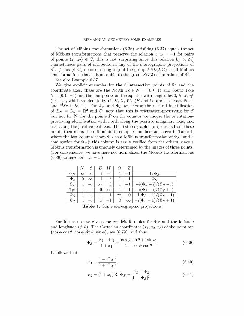
See also Example 6.37.We give explicit examples for the 6 intersection points of S2 and the
coordinate axes; these are the North Pole N = (0, 0, 1) and South PoleS = (0, 0,−1) and the four points on the equator with longitudes 0, π2 , π, 3π
2(or −π
2 ), which we denote by O, E, Z, W . (E and W are the “East Pole”and “West Pole”.) For ΦN and ΦS we choose the natural identificationof LN = LS = R2 and C; note that this is orientation-preserving for Sbut not for N ; for the points P on the equator we choose the orientation-preserving identification with north along the positive imaginary axis, andeast along the positive real axis. The 6 stereographic projections from thesepoints then maps these 6 points to complex numbers as shown in Table 1,where the last column shows ΦP as a Mobius transformation of ΦS (and aconjugation for ΦN ); this column is easily verified from the others, since aMobius transformation is uniquely determined by the images of three points.(For convenience, we have here not normalized the Mobius transformations(6.36) to have ad− bc = 1.)
N S E W O Z
ΦN ∞ 0 i −i 1 −1 1/ΦS
ΦS 0 ∞ i −i 1 −1 ΦS
ΦE i −i ∞ 0 1 −1 −i(ΦS + i)/(ΦS − i)ΦW i −i 0 ∞ −1 1 −i(ΦS − i)/(ΦS + i)ΦO i −i −1 1 ∞ 0 −i(ΦS + 1)/(ΦS − 1)ΦZ i −i 1 −1 0 ∞ −i(ΦS − 1)/(ΦS + 1)
Table 1. Some stereographic projections
For future use we give some explicit formulas for ΦZ and the latitudeand longitude (φ, θ). The Cartesian coordinates (x1, x2, x3) of the point are(cosφ cos θ, cosφ sin θ, sinφ
), see (6.79), and thus
ΦZ =x2 + ix3
1 + x1=
cosφ sin θ + i sinφ
1 + cosφ cos θ. (6.39)
It follows that
x1 =1− |ΦZ |2
1 + |ΦZ |2, (6.40)
x2 = (1 + x1) Re ΦZ =ΦZ + ΦZ
1 + |ΦZ |2, (6.41)

32 SVANTE JANSON
x3 = (1 + x1) Im ΦZ = −iΦZ − ΦZ
1 + |ΦZ |2. (6.42)
(6.43)
Since sinφ = x3, cosφ cos θ = x1 and cosφ sin θ = x2, elementary calcula-tions yield
sinφ = −iΦZ − ΦZ
1 + |ΦZ |2, (6.44)
cosφ =|1 + Φ2
Z |1 + |ΦZ |2
, (6.45)
cos θ =1− |ΦZ |2
|1 + Φ2Z |, (6.46)
sin θ =ΦZ + ΦZ
|1 + Φ2Z |. (6.47)
Example 6.5 (Gnomonic (central) projection). The gnomonic projectionprojects the sphere Sn from the centre 0 to a tangent plane. Obviously, sucha map projection cannot distinguish between antipodes, so it is limited to ahemisphere.5
We choose to project the upper hemisphere ξ ∈ Sn : ξn+1 > 0 onto thetangent plane at the North Pole (x, 1) : x ∈ Rn ⊂ Rn+1. We thus map apoint (ξ′, ξn+1) ∈ Sn with ξn+1 > 0 to
Ψ(ξ′, ξn+1) =ξ′
ξn+1∈ Rn. (6.48)
The inverse map is
Ψ−1(x) =(x, 1)√1 + |x|2
. (6.49)
A small calculation shows that the metric is
|ds|2 =|dx|2
1 + |x|2− |〈dx, x〉|
2
(1 + |x|2)2=|dx|2 + |x ∧ dx|2
(1 + |x|2)2, (6.50)
i.e.,
gij =δij
1 + |x|2− xixj
(1 + |x|2)2. (6.51)
5The gnomonic projection is also one of the oldest used in cartography. It is usefulfor long-distance navigation, e.g. for intercontinental flights, since it shows geodesics (theshortest paths) as straight lines (this includes the equator and all meridians) [16, p. 169].
“It was used by Thales (636?–546?B.C.) of Miletus for star maps. Called ”horologium”(sundial or clock) in early times, it was given the name ”gnomonic” in the 19th century.It has also been called the Gnomic and the Central projection. The name Gnomonic isderived from the fact that the meridians radiate from the pole (or are spaced, on theequatorial aspect) just as the corresponding hour markings on a sundial for the samecentral latitude. The gnomon of the sundial is the elevated straightedge pointed towardthe pole and casting its shadow on the various hour markings as the sun moves across thesky.” [15, p. 164]

RIEMANNIAN GEOMETRY: SOME EXAMPLES 33
The metric is thus not conformal. The inverse matrix is, see Lemma E.1,
gij = (1 + |x|2)(δij + xixj). (6.52)
The determinant is, again using Lemma E.1,
|g| = (1 + |x|2)−n−1, (6.53)
and the invariant measure (1.6) is thus
dµ = (1 + |x|2)−(n+1)/2 dx1 · · · dxn. (6.54)
The volume scale is thus (1 + |x|2)(n+1)/2.By (6.50)–(6.51), the largest and smallest eigenvalues of gij are (1+|x|2)−1
and (1 + |x|2)−2, respectively, and thus the condition number is
κ = 1 + |x|2. (6.55)
By (1.7), the eccentricity is
ε =|x|√
1 + |x|2. (6.56)
Calculations yield
Γkij = −xiδjk + xjδik(1 + |x|2)2
+2xixjxk
(1 + |x|2)3= −
xigjk + xjgik1 + |x|2
, (6.57)
Γkij = −xiδjk + xjδik
1 + |x|2(6.58)
The connection is of the form (1.37), and thus the geodesics are Euclideanlines; this is also obvious geometrically, since the geodesics on the sphere areintersections of the sphere with 2-dimensional planes through the centre,which project to the intersection of the plane with the plane (x, 1) : x ∈Rn, which is a line in that plane. The equation (1.36) for a geodesic becomes
γi =2∑
j γj γj
1 + |γ|2γi =
d log(1 + |γ|2)
dtγi. (6.59)
A geodesic can be parametrized (with unit speed) as
γ(t) = x+ tan(t) · v (6.60)
where x = γ(0) ∈ Rn, v = γ(0) ∈ Rn with x ⊥ v and |v|2 = 1 + |x|2.The gnomonic projection evidently maps a circle on the sphere to a conic
section, i.e., a circle, an ellipse, a parabola or (one branch of) a hyperbola,or (in the case of a geodesic) a straight line. (Of course, only the part of thecircle in the upper hemisphere is mapped.)
Example 6.6 (Orthogonal (orthographic) projection). The orthogonal pro-jection of the sphere Sn onto Rn is in cartography called the orthographic
34 SVANTE JANSON
projection.6 The orthogonal (orthographic) projection is thus the map
(ξ′, ξn+1) 7→ ξ′. (6.61)
This is a diffeomorphism in each of the two hemispheres ξn+1 > 0 andξn+1 < 0, mapping each of them onto the open unit ball x : |x| < 1 in Rn;if we choose to regard it as a map from the upper hemisphere, its inverse is
x 7→(x,√
1− |x|2), |x| < 1. (6.62)
A small calculation shows that the metric is
|ds|2 = |dx|2 +|〈dx, x〉|2
1− |x|2(6.63)
i.e.,
gij = δij +xixj
1− |x|2. (6.64)
The metric is thus not conformal. By Lemma E.1, the determinant is
|g| = 1 +|x|2
1− |x|2=
1
1− |x|2, (6.65)
and the inverse matrix isgij = δij − xixj . (6.66)
The invariant measure (1.6) is thus
dµ = (1− |x|2)−1/2 dx1 · · · dxn. (6.67)
I.e., the volume scale is (1− |x|2)1/2.By (6.63)–(6.64), the largest and smallest eigenvalues of gij are (1−|x|2)−1
and 1, respectively, and thus the condition number is
κ = (1− |x|2)−1. (6.68)
6This is how the sphere looks from a great distance, for example (approximatively) theearth seen (or photographed) from the moon; conversely, this is how we see the surface ofthe moon.
“To the layman, the best known perspective azimuthal projection is the Orthographic,although it is the least useful for measurements. While its distortion in shape and area isquite severe near the edges, and only one hemisphere may be shown on a single map, theeye is much more willing to forgive this distortion than to forgive that of the Mercatorprojection because the Orthographic projection makes the map look very much like aglobe appears, especially in the oblique aspect.
The Egyptians were probably aware of the Orthographic projection, and Hipparchusof Greece (2nd century B.C.) used the equatorial aspect for astronomical calculations.Its early name was ”analemma,” a name also used by Ptolemy, but it was replaced by”orthographic” in 1613 by Francois d’ Aiguillon of Antwerp. While it was also used byIndians and Arabs for astronomical purposes, it is not known to have been used for worldmaps older than 16th-century works by Albrecht Durer (1471–1528), the German artistand cartographer, who prepared polar and equatorial versions.” [15, p. 145]
“The Roman architect and engineer Marcus Vitruvius Pollio, ca. 14 B.C., used it toconstruct sundials and to compute sun positions.” Vitruvius also, apparently, originatedthe term orthographic. [16, p. 17]
See also [16, p. 170] for modern use.

RIEMANNIAN GEOMETRY: SOME EXAMPLES 35
By (1.7), the eccentricity is
ε = |x|. (6.69)
Calculations yield
Γkij =xkδij
1− |x|2+
xixjxk(1− |x|2)2
=xkgij
1− |x|2, (6.70)
Γkij = xkgij . (6.71)
Example 6.7 (Polar coordinates on a sphere). Consider Example 4.5 withw(r) = sin r, r ∈ (0, π). Then w′′/w = −1, and (4.27) shows that M hasconstant curvature 1.
In fact, if M = (0, π)× (θ0, θ0 + 2π), for some θ0 ∈ R, then
(r, θ) 7→ (sin r cos θ, sin r sin θ, cos r) (6.72)
is an isometry ofM onto S2\`, where ` is the meridian (sin r cos θ0, sin r sin θ0,cos r) : r > 0. r is the distance to the North Pole N = (0, 0, 1), so this ispolar coordinates on the sphere S2 with the North Pole as centre. In thiscontext, r is usually denoted ϕ; ϕ = r is called the polar angle (or zenithangle or colatitude); it is the angle from the North Pole N , seen from thecentre of the sphere. The map (6.72) to S2 is thus
(ϕ, θ) 7→ (sinϕ cos θ, sinϕ sin θ, cosϕ). (6.73)
The metric tensor is, using the notation (ϕ, θ),
g11 = 1, g12 = g21 = 0, g22 = sin2 ϕ, (6.74)
or in matrix form
(gij) =
(1 00 sin2 ϕ
). (6.75)
The connection coefficients are, by (4.22)–(4.23),
Γ122 = − sinϕ cosϕ, (6.76)
Γ212 = Γ2
21 = cotϕ, (6.77)
with all other components 0. The invariant measure is
dµ = sinϕdϕdθ. (6.78)
Example 6.8 (Latitude and longitude). Latitude and longitude, the tra-ditional coordinate system on a sphere,7 is the pair of coordinates (φ, θ)obtained from the coordinates (ϕ, θ) in Example 6.7 by φ := π/2 − ϕ; inother words, the point (φ, θ) has Cartesian coordinates(
cosφ cos θ, cosφ sin θ, sinφ). (6.79)
7First used in a formalized way by Hipparchus from Rhodes (ca. 190–after 126 B.C.)[16, p. 4].
36 SVANTE JANSON
We take φ ∈ [−π/2, π/2]. Traditionally, either θ ∈ [−π, π] (with negativevalues West and positive values East) or θ ∈ [0, 2π);8 for a coordinate mapin differential geometry sense we take φ ∈ (−π/2, π/2) and θ ∈ (θ0, θ0 +2π),omitting a meridian.9
The metric tensor is, e.g. by (6.74),
g11 = 1, g12 = g21 = 0, g22 = cos2 φ, (6.80)
or in matrix form
(gij) =
(1 00 cos2 φ
). (6.81)
This is another instance of Example 4.5, now with (using φ instead ofr) w(φ) = cosφ, φ ∈ (−π/2, π/2). We again have w′′/w = −1, and (4.27)shows again that the sphere S2 has constant curvature 1.
The connection coefficients are, by (4.22)–(4.23),
Γ122 = sinφ cosφ, (6.82)
Γ212 = Γ2
21 = − tanφ, (6.83)
with all other components 0. The invariant measure is
dµ = cosφ dφ dθ. (6.84)
Example 6.9 (Equirectangular projection). This is simply the coordinates(φ, aθ), where a > 0 is a constant. This is thus obtained from latitude andlongitude by scaling one of the coordinates. Meridians and parallels (spacedat, say, 1) form two perpendicular families of parallel lines, each of themuniformly spaced, which thus together form rectangles of equal size.10
The special case a = 1 is thus just (φ, ϕ) as in Example 6.8; in this case,meridians and parallels form squares. As a map projection, this special caseis called plate carree or plane chart. [16, p. 5].11
8More precisely, [−180, 180] or [0, 360), since traditionally degrees are used. (As-tronomers sometimes also use [0h, 24h).) In geography, [−180, 180] is standard, whileastronomers use [0, 360) [1, pp. 11 and 203].
0 is currently at the meridian through Greenwich; various other standard meridianshave been used on older maps. On the celestial sphere, 0 is at the vernal equinox (firstpoint of Aries).
Similarly, latitude is traditionally given in [−90, 90], with positive values North andnegative values South.
9Coordinates are traditionally given in the order (φ, θ), but maps are plotted withthe coordinates in the order (θ, φ), i.e., with the longitude along the x-axis. We ignorethis trivial difference. In other words, we regard maps as plotted with the x-axis verti-cal (North) and the y-axis horizontal (East). (The same applies to several projectionsdiscussed below.)
10This explains the name equirectangular or rectangular projection. This projectionwas invented by Marinus of Tyre about 100 A.D., and was widely used until the 17thcentury; it has also some modern use [16, pp. 4–5, 158]
11The transverse form of plate caree is called Cassini’s projection. It was invented in1745 (in the ellipsoidal version) by Cesar Francois Cassini de Thury (1714–1784), and has
RIEMANNIAN GEOMETRY: SOME EXAMPLES 37
The metric tensor is by (6.80),
g11 = 1, g12 = g21 = 0, g22 = a−2 cos2 φ, (6.85)
or in matrix form
(gij) =
(1 00 a−2 cos2 φ
). (6.86)
Note that if a = cosϕ0 for some ϕ0 ∈ [0, π/2) (and thus 0 < a 6 1), thengij = δij when ϕ = ±ϕ0, so the map is locally conformal and isometric atlatitude ϕ = ±ϕ0; these parallels are called standard parallels. In particular,with a = 1 as in Example 6.8, the equator is the standard parallel.
The metric (6.85) is another instance of Example 4.5, now with (using φinstead of r) w(φ) = a cosφ, φ ∈ (−π/2, π/2). We again have w′′/w = −1,and (4.27) shows again that the sphere S2 has constant curvature 1.
The connection coefficients are, by (4.22)–(4.23),
Γ122 = a2 sinφ cosφ, (6.87)
Γ212 = Γ2
21 = − tanφ, (6.88)
with all other components 0. The invariant measure is
dµ = a cosφ dφ dθ. (6.89)
The area scale is thus a−1 cos−1 φ.By (6.85), the condition number is
κ = max(a−2 cos2 ϕ, a2 cos−2 ϕ
). (6.90)
If a = cosϕ0, we see again that κ = 1, and thus ε = 0, if and only ifϕ = ±ϕ0.
Example 6.10 (Cylindrical projections). Let (φ, θ) be the latitude andlongitude as in Example 6.8 and consider the transformation ζ = ζ(φ) ofthe latitude, where ζ is a smooth function with (smooth) inverse φ(ζ). Thisyields the coordinates
(ζ, θ) = (ζ(φ), θ) (6.91)
on S2. A map projection of this type is called a cylindrical projection. Themetric tensor is by (6.80)
g11 = (φ′(ζ))2, g12 = g21 = 0, g22 = cos2(φ(ζ)). (6.92)
This is a metric of the type in Example 4.7.The meridians are equispaced vertical lines and the parallels are hori-
zontal lines (but not necessarily equispaced). In particular, meridians andparallels are orthogonal to each other; however, the projection in general
been used in several countries, in particular during the 19th century [16, pp. 74–76, 97,159].
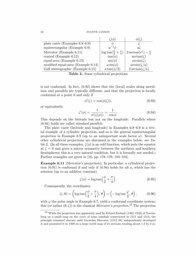
38 SVANTE JANSON
ζ(φ) φ(ζ)plate caree (Examples 6.8–6.9) φ ζequirectangular (Example 6.9) a−1φ aζ
Mercator (Example 6.11) log tan(φ2 + π4 ) 2 arctan(eζ)− π
2central (Example 6.12) tan(φ) arctan(ζ)equal-area (Example 6.13) sin(φ) arcsin(ζ)modified equal-area (Example 6.14) a sin(φ) arcsin(ζ/a)Gall stereographic (Example 6.15) a tan(φ/2) 2 arctan(ζ/a)
Table 2. Some cylindrical projections
is not conformal. In fact, (6.92) shows that the (local) scales along merid-ians and parallels are typically different, and that the projection is locallyconformal at a point if and only if
φ′(ζ) = cos(φ(ζ)), (6.93)
or equivalently
ζ ′(φ) =1
φ′(ζ(φ))=
1
cosφ. (6.94)
This depends on the latitude but not on the longitude. Parallels where(6.94) holds are called standard parallels.
The plate caree (latitude and longitude) in Examples 6.8–6.9 is a triv-ial example of a cylindric projection, and so is the general equirectangularprojection in Example 6.9 (up to an unimportant scale factor a). Severalother cylindrical projections are discussed in the examples below, see Ta-ble 2. (In all these examples, ζ(φ) is an odd function, which puts the equatorat ζ = 0 and gives a mirror symmetry between the northern and southernhemispheres; this is a very natural condition, but it is formally not needed.)Further examples are given in [16, pp. 178–179, 183–184].
Example 6.11 (Mercator’s projection). In particular, a cylindrical projec-tion (6.91) is conformal if and only if (6.94) holds for all φ, which has thesolution (up to an additive constant)
ζ(φ) = log tan(φ
2+π
4
). (6.95)
Consequently, the coordinates
(ζ, θ) =
(log tan
(φ2
+π
4
), θ
)=(− log tan
ϕ
2, θ), (6.96)
with ϕ the polar angle in Example 6.7, yield a conformal coordinate system;this (or rather (θ, ζ)) is the classical Mercator’s projection.12 The projection
12“While the projection was apparently used by Erhard Etzlaub (1462–1532) of Nurem-berg on a small map on the cover of some sundials constructed in 1511 and 1513, theprinciple remained obscure until Gerardus Mercator (1512–94) independently developedit and presented it in 1569 on a large world map of 21 sections totaling about 1.3 by 2 m.

RIEMANNIAN GEOMETRY: SOME EXAMPLES 39
composed with a rotation of the sphere, so that the equator of the projectionis a meridian on the sphere, is called the transverse Mercator projection orthe Gauss conformal projection.13
If we regard the stereographic projection ΦN from the North Pole inExample 6.2 as a mapping into the complex plane, then a point with coor-dinates (ϕ, θ) on the sphere is by (6.27) mapped to ΦN (ϕ, θ) = cot ϕ2 · e
iθ
and thus (6.96) can be written
ζ + iθ = log ΦN (ϕ, θ). (6.97)
In other words, Mercator’s projection equals the (complex) logarithm of thestereographic projection. (This yields another proof that the projection isconformal, since the stereographic projection is.) With the stereographicprojection ΦS in Example 6.1, the same holds except that the sign of ζ hasto be reversed.
The change of coordinates (6.96) can be expressed in different ways. Wehave, for example,
sinφ = cosϕ = tanh ζ, (6.98)
His 1569 map is entitled ”Nova et Aucta Orbis Terrae Descriptio ad Usum NavigantiumEmendate Accommodata (A new and enlarged description of the Earth with correctionsfor use in navigation).” He described in Latin the nature of the projection in a large panelcovering much of his portrayal of North America:
In this mapping of the world we have [desired] to spread out the surface of the globeinto a plane that the places shall everywhere be properly located, not only with respectto their true direction and distance, one from another, but also in accordance with theirdue longitude and latitude; and further, that the shape of the lands, as they appearon the globe, shall be preserved as far as possible. For this there was needed a newarrangement and placing of meridians, so that they shall become parallels, for the mapshitherto produced by geographers are, on account of the curving and the bending of themeridians, unsuitable for navigation Taking all this into consideration, we have somewhatincreased the degrees of latitude toward each pole, in proportion to the increase of theparallels beyond the ratio they really have to the equator” [15, p. 38]
The main practical feature for navigation is that meridians are parallel and that sailingroutes keeping a constant direction with respect to North are shown as straight lines.These lines are called loxodromes or rhumb lines; they are not geodesics, i.e. the shortestpaths (unless on a meridian or the equator), but they are convenient for navigation. Onthe other hand, distances and the area are much distorted at high latitudes as shown by(6.102)–(6.103) and (6.99). See [15, p. 39–41].
Mercator’s projection is thus the only projection really suitable for navigation (at leastbefore the GPS), and it its thus used for nautical charts. It is also often used for otherpurposes, such as world maps, where it really is a bad choice; it may be attractive for wallcharts because it is rectangular, but it has large distortions at high (and even not so high)latitudes. See also [16, p. 156–157].
13It was really invented by Johann Heinrich Lambert in 1772 (together with six othermap projections, see [16, p. 76] and Examples 6.13, 6.18, 6.26, 6.27); the version forellipsoids was analyzed by Carl Friedrich Gauss in 1822, and further by L. Kruger in 1912;hence it is (in the ellipsoidal version) also called the Gauss–Kruger projection. It is oneof the most widely used map projections, since it is conformal but has small distortionson an area that does not extend too far from the central meridian. [15, p. 48, 51], [16,p. 159–161]
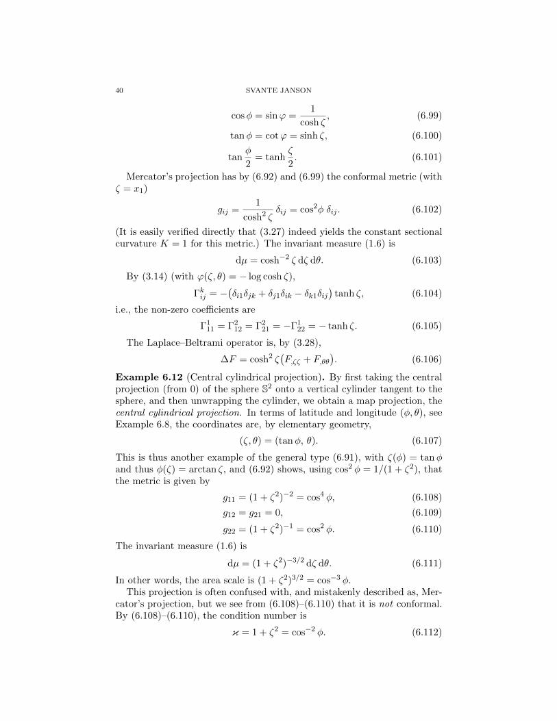
40 SVANTE JANSON
cosφ = sinϕ =1
cosh ζ, (6.99)
tanφ = cotϕ = sinh ζ, (6.100)
tanφ
2= tanh
ζ
2. (6.101)
Mercator’s projection has by (6.92) and (6.99) the conformal metric (withζ = x1)
gij =1
cosh2 ζδij = cos2φ δij . (6.102)
(It is easily verified directly that (3.27) indeed yields the constant sectionalcurvature K = 1 for this metric.) The invariant measure (1.6) is
dµ = cosh−2 ζ dζ dθ. (6.103)
By (3.14) (with ϕ(ζ, θ) = − log cosh ζ),
Γkij = −(δi1δjk + δj1δik − δk1δij
)tanh ζ, (6.104)
i.e., the non-zero coefficients are
Γ111 = Γ2
12 = Γ221 = −Γ1
22 = − tanh ζ. (6.105)
The Laplace–Beltrami operator is, by (3.28),
∆F = cosh2 ζ(F,ζζ + F,θθ
). (6.106)
Example 6.12 (Central cylindrical projection). By first taking the centralprojection (from 0) of the sphere S2 onto a vertical cylinder tangent to thesphere, and then unwrapping the cylinder, we obtain a map projection, thecentral cylindrical projection. In terms of latitude and longitude (φ, θ), seeExample 6.8, the coordinates are, by elementary geometry,
(ζ, θ) = (tanφ, θ). (6.107)
This is thus another example of the general type (6.91), with ζ(φ) = tanφand thus φ(ζ) = arctan ζ, and (6.92) shows, using cos2 φ = 1/(1 + ζ2), thatthe metric is given by
g11 = (1 + ζ2)−2 = cos4 φ, (6.108)
g12 = g21 = 0, (6.109)
g22 = (1 + ζ2)−1 = cos2 φ. (6.110)
The invariant measure (1.6) is
dµ = (1 + ζ2)−3/2 dζ dθ. (6.111)
In other words, the area scale is (1 + ζ2)3/2 = cos−3 φ.This projection is often confused with, and mistakenly described as, Mer-
cator’s projection, but we see from (6.108)–(6.110) that it is not conformal.By (6.108)–(6.110), the condition number is
κ = 1 + ζ2 = cos−2 φ. (6.112)

RIEMANNIAN GEOMETRY: SOME EXAMPLES 41
By (1.7), the eccentricity is
ε =|ζ|√
1 + ζ2= | sinφ|. (6.113)
The metric (6.108)–(6.110) is an example of Example 4.7, and it followsfrom (4.60) that the non-zero components Γkij of the connection are
Γ111 = − 2ζ
1 + ζ2, Γ1
22 = ζ, Γ212 = Γ2
21 = − ζ
1 + ζ2. (6.114)
Example 6.13 (Lambert cylindrical equal-area projection). By first pro-jecting the sphere S2 radially from the z-axis (keeping z fixed) to a tangentvertical cylinder, and then unwrapping the cylinder, we obtain the Lam-bert cylindrical equal-area projection.14 (Do not confuse with Example 6.12,which is quite different.) In terms of latitude and longitude (φ, θ), see Ex-ample 6.8, the coordinates are, by elementary geometry, cf. (6.107),
(ζ, θ) = (sinφ, θ). (6.115)
This is thus another example of the general type (6.91), with ζ(φ) = sinφand thus φ(ζ) = arcsin ζ, and (6.92) shows, using cos2 φ = 1 − ζ2, thatthe metric is given by (note that we have |ζ| = | sinφ| < 1 for this mapprojection)
g11 = (1− ζ2)−1 = cos−2 φ, (6.116)
g12 = g21 = 0, (6.117)
g22 = 1− ζ2 = cos2 φ. (6.118)
Consequently,
|g| = g11g22 = 1, (6.119)
and the invariant measure (1.6) is
dµ = dζ dθ, (6.120)
i.e., the coordinates (6.115) are area-preserving. (This is a well-known geo-metric fact.)
By (6.116)–(6.118), the condition number is
κ = (1− ζ2)−2 = cos−4 φ. (6.121)
By (1.7), the eccentricity is
ε =√
1− (1− ζ2)2 = |ζ|√
2− ζ2. (6.122)
The metric (6.116)–(6.118) is an example of Example 4.7, and it followsfrom (4.60) that the non-zero components Γkij of the connection are
Γ111 =
ζ
1− ζ2, Γ1
22 = ζ(1− ζ2), Γ212 = Γ2
21 = − ζ
1− ζ2. (6.123)
14Invented by Johann Heinrich Lambert 1772. [15, p. 76]

42 SVANTE JANSON
Example 6.14 (Modified cylindrical equal-area projection). The cylindricalequal-area projection (6.115) is conformal on the equator, φ = 0, i.e., for ζ =0, since then g11 = g22, see (6.116)–(6.118). The projection can be modifiedby a non-isotropic scaling to (a sinϕ, bθ) with a, b > 0; we choose (withoutloss of generality up to a linear scaling) a = 1, and take b = cos2 φ0 ∈ (0, 1]for some φ0 ∈ [0, π/2). The coordinates are thus
(ζ, bθ) = (sinφ, bθ) = (sinφ, θ cos2 φ0). (6.124)
The metric tensor is, cf. (6.116)–(6.118), for |ζ| = | sinφ| < 1,
g11 =1
1− ζ2= cos−2 φ, (6.125)
g12 = g21 = 0, (6.126)
g22 = b−2(1− ζ2) =1− ζ2
cos4 φ0=
cos2 φ
cos4 φ0. (6.127)
Hence the metric is conformal at the points where ζ2 = 1− b = sin2 φ0, i.e.,at latitude φ = ±φ0. In other words, the projection (6.124) has standardparallels ±φ0.
The case φ0 = 0 (b = 1) yields the Lambert cylindrical equal-area pro-jection in Example 6.13. The case φ0 = 45 (b = 1/2) is called the Gall(orthographic) projection or Peters projection or (as a compromise) Gall–Peters projection (it was invented by Gall 1855 and reinvented by Peters1973 with exaggerated claims and publicity). The case φ0 = 30 (b = 3/4)is called the Behrmann projection.15
Geometrically, this projection can be described by first taking the radialprojection from the z-axis to a vertical cylinder with radius b = cos2 φ, andthen unwrapping the cylinder; cf. Example 6.13.
By (6.125)–(6.127),
|g| = g11g22 = b−2 = (cosφ0)−4 (6.128)
15“The earliest such modification is from Scotland: James Gall’s Orthographic Cylin-drical, not the same as his preferred Stereographic Cylindrical, both of which were orig-inated in 1855, has standard parallels of 45 N. and S. (Gall, 1885). Walther Behrmann(1910) of Germany chose 30, based on certain overall distortion criteria. Very similarlater projections were offered by Trystan Edwards of England in 1953 and Arno Petersof Germany in 1967; they were presented as revolutionary and original concepts, ratherthan as modifications of these prior projections with standard parallels at about 37 and45–47, respectively.” [15, p. 76]
“There is extreme shape and scale distortion 90 from the central line, or at the poleson the normal aspect. These are the points which have infinite area and linear scale onthe various aspects of the Mercator projection. This distortion, even on the modificationsdescribed above, is so great that there has been little use of any of the forms for world mapsby professional cartographers, and many of them have strongly criticized the intensivepromotion in the noncartographic community which has accompanied the presentation ofone of the recent modifications.” [15, p. 77]
See also [16, p. 164–166] for a discussion of the controversy around Peters’ claims.

RIEMANNIAN GEOMETRY: SOME EXAMPLES 43
is constant and the invariant measure (1.6) is
dµ = b−1 dζ dθ = (cosφ0)−2 dζ dθ, (6.129)
i.e., the coordinates (6.124) are area-preserving up to a constant factor. (Weobtain equal area by multiplying the coordinates (6.124) by 1/ cosφ0, i.e.,for the coordinates (
sinφ/ cosφ0, θ cosφ0
), (6.130)
but we prefer to use (6.124).)The transformation from (6.116)–(6.118) to (6.125)–(6.127) is an exam-
ple of Example 4.8, and it follows from (4.60) or (4.67) that the non-zerocomponents Γkij of the connection are
Γ111 =
ζ
1− ζ2, Γ1
22 = b−2ζ(1− ζ2), Γ212 = Γ2
21 = − ζ
1− ζ2. (6.131)
The sectional curvature K = −1 by (4.69).This projection (or rather (bθ, sinφ)) maps the sphere to a rectangle with
aspect ratio width/heigth = bπ.
Example 6.15 (The Gall stereographic projection). In the Gall stereo-graphic projection, the sphere (except for the poles) is projected onto acylinder, which then is unwrapped (as in Examples 6.12–6.14); each merid-ian is projected using a perspective projection from the point on the equatoropposite to the meridian.16 Furthermore, the cylinder is chosen to intersectthe sphere at two standard parallels ±φ0, and has thus radius cosφ0.17
In terms of latitude and longitude (φ, θ), see Example 6.8, the coordinatesare, by elementary geometry,
(ζ, θ) =(
(1 + cosφ0) tanφ
2, cosφ0 · θ
). (6.132)
If we divide by the scale factor cosϕ0 (thus making the scale correct alongthe equator instead of along the standard parallel, this becomes anotherexample of the general type (6.91), with
ζ(φ) = a tanφ
2, (6.133)
where
a =1 + cosφ0
cosφ0. (6.134)
Thus φ(ζ) = 2 arctan(ζ/a), and (6.92) shows that the metric is given by
g11 =( 2a
a2 + ζ2
)2=(1 + cosφ
a
)2, (6.135)
g12 = g21 = 0, (6.136)
16The projection is thus not a perspective projection from some fixed point.17This projection was proposed by Gall in 1855, with standard parallels φ0 = 45;
versions with standard parallels 55 and 30 have later been used in the Soviet Union.[16, pp. 108–110, 163–164]
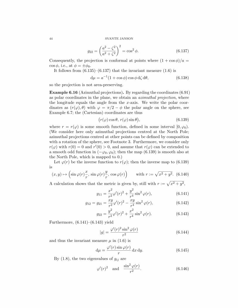
44 SVANTE JANSON
g22 =
(a2 − ζ2
a2 + ζ2
)2
= cos2 φ. (6.137)
Consequently, the projection is conformal at points where (1 + cosφ)/a =cosφ, i.e., at φ = ±φ0.
It follows from (6.135)–(6.137) that the invariant measure (1.6) is
dµ = a−1(1 + cosφ) cosφ dζ dθ, (6.138)
so the projection is not area-preserving.
Example 6.16 (Azimuthal projections). By regarding the coordinates (6.91)as polar coordinates in the plane, we obtain an azimuthal projection, wherethe longitude equals the angle from the x-axis. We write the polar coor-dinates as (r(ϕ), θ) with ϕ = π/2 − φ the polar angle on the sphere, seeExample 6.7; the (Cartesian) coordinates are thus(
r(ϕ) cos θ, r(ϕ) sin θ), (6.139)
where r = r(ϕ) is some smooth function, defined in some interval [0, ϕ0).(We consider here only azimuthal projections centred at the North Pole;azimuthal projections centred at other points can be defined by compositionwith a rotation of the sphere, see Footnote 3. Furthermore, we consider onlyr(ϕ) with r(0) = 0 and r′(0) > 0, and assume that r(ϕ) can be extended toa smooth odd function in (−ϕ0, ϕ0); then the map (6.139) is smooth also atthe North Pole, which is mapped to 0.)
Let ϕ(r) be the inverse function to r(ϕ); then the inverse map to (6.139)is
(x, y) 7→(
sinϕ(r)x
r, sinϕ(r)
y
r, cosϕ(r)
)with r :=
√x2 + y2. (6.140)
A calculation shows that the metric is given by, still with r :=√x2 + y2,
g11 =x2
r2ϕ′(r)2 +
y2
r4sin2 ϕ(r), (6.141)
g12 = g21 =xy
r2ϕ′(r)2 − xy
r4sin2 ϕ(r), (6.142)
g22 =y2
r2ϕ′(r)2 +
x2
r4sin2 ϕ(r). (6.143)
Furthermore, (6.141)–(6.143) yield
|g| = ϕ′(r)2 sin2 ϕ(r)
r2(6.144)
and thus the invariant measure µ in (1.6) is
dµ =ϕ′(r) sinϕ(r)
rdx dy. (6.145)
By (1.8), the two eigenvalues of gij are
ϕ′(r)2 andsin2 ϕ(r)
r2. (6.146)

RIEMANNIAN GEOMETRY: SOME EXAMPLES 45
r(ϕ) ϕ(r)stereographic (Example 6.1) tan(ϕ/2) 2 arctan(r)stereographic (Example 6.3) 2 tan(ϕ/2) 2 arctan(r/2)gnomonic (Example 6.5) tan(ϕ) arctan(r)orthographic (Example 6.6) sin(ϕ) arcsin(r)equidistant (Example 6.17) ϕ requal-area (Example 6.18) 2 sin(ϕ/2) 2 arcsin(r/2)Breusing harmonic (Example 6.21) 4 tan(ϕ/4) 4 arctan(r/4)
Table 3. Some azimuthal projections
Note that the stereographic projection in Example 6.1 is the special caser = tan(ϕ/2), see (6.23), and thus ϕ(r) = 2 arctan r. Similarly, the al-ternative stereographic projection in Example 6.3, the gnomonic projectionin Example 6.5 and the orthographic projection in Example 6.6 are specialcases, see Table 3; it is easily verified that (6.141)–(6.143) yield (6.7), (6.30),(6.51) and (6.64) for these cases. We give further examples in the followingexamples.
Example 6.17 (Azimuthal equidistant projection). By taking r = ϕ inExample 6.16, the distances from the centre point (the North Pole) arepreserved; this projection thus gives correct directions and distances froma fixed point, and it is therefore called the azimuthal equidistant projection.(Of course, distances between other points are not preserved.)18
We have 0 6 r < π; the sphere minus the South Pole is mapped diffeo-morphically onto the open disc with radius π. (The South Pole has ϕ = π,but θ is undetermined, and we cannot define the map to include the SouthPole in any continuous manner.)
The metric is by (6.141)–(6.143) given by, with r :=√x2 + y2,
g11 =x2
r2+y2 sin2 r
r4, (6.147)
g12 = g21 =xy(r2 − sin2 r)
r4, (6.148)
18One example is the United Nations flag and emblem, showing a map in azimuthalequidistant projection centred on the North Pole, extending to 60 south and inscribed ina wreath. [17] See [16, p. 170–172] for other modern examples.
“The Azimuthal Equidistant was apparently used centuries before the 15th-centurysurge in scientific mapmaking. It is believed that Egyptians used the polar aspect forstar charts, but the oldest existing celestial map on the projection was prepared in 1426by Conrad of Dyffenbach. It was also used in principle for small areas by mariners fromearliest times in order to chart coasts, using distances and directions obtained at sea.The first clear examples of the use of the Azimuthal Equidistant for polar maps of theEarth are those included by Gerardus Mercator as insets on his 1569 world map, whichintroduced his famous cylindrical projection. As Northern and Southern Hemispheres, theprojection appeared in a manuscript of about 1510 by the Swiss Henricus Loritus, usuallycalled Glareanus (1488–1563), and by several others in the next few decades.” [15, p. 191]
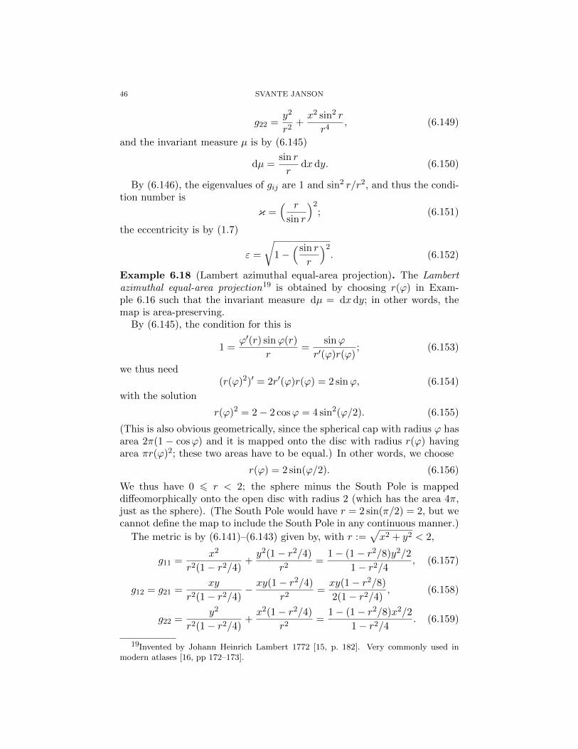
46 SVANTE JANSON
g22 =y2
r2+x2 sin2 r
r4, (6.149)
and the invariant measure µ is by (6.145)
dµ =sin r
rdx dy. (6.150)
By (6.146), the eigenvalues of gij are 1 and sin2 r/r2, and thus the condi-tion number is
κ =( r
sin r
)2; (6.151)
the eccentricity is by (1.7)
ε =
√1−
(sin r
r
)2. (6.152)
Example 6.18 (Lambert azimuthal equal-area projection). The Lambertazimuthal equal-area projection19 is obtained by choosing r(ϕ) in Exam-ple 6.16 such that the invariant measure dµ = dx dy; in other words, themap is area-preserving.
By (6.145), the condition for this is
1 =ϕ′(r) sinϕ(r)
r=
sinϕ
r′(ϕ)r(ϕ); (6.153)
we thus need(r(ϕ)2)′ = 2r′(ϕ)r(ϕ) = 2 sinϕ, (6.154)
with the solution
r(ϕ)2 = 2− 2 cosϕ = 4 sin2(ϕ/2). (6.155)
(This is also obvious geometrically, since the spherical cap with radius ϕ hasarea 2π(1 − cosϕ) and it is mapped onto the disc with radius r(ϕ) havingarea πr(ϕ)2; these two areas have to be equal.) In other words, we choose
r(ϕ) = 2 sin(ϕ/2). (6.156)
We thus have 0 6 r < 2; the sphere minus the South Pole is mappeddiffeomorphically onto the open disc with radius 2 (which has the area 4π,just as the sphere). (The South Pole would have r = 2 sin(π/2) = 2, but wecannot define the map to include the South Pole in any continuous manner.)
The metric is by (6.141)–(6.143) given by, with r :=√x2 + y2 < 2,
g11 =x2
r2(1− r2/4)+y2(1− r2/4)
r2=
1− (1− r2/8)y2/2
1− r2/4, (6.157)
g12 = g21 =xy
r2(1− r2/4)− xy(1− r2/4)
r2=xy(1− r2/8)
2(1− r2/4), (6.158)
g22 =y2
r2(1− r2/4)+x2(1− r2/4)
r2=
1− (1− r2/8)x2/2
1− r2/4. (6.159)
19Invented by Johann Heinrich Lambert 1772 [15, p. 182]. Very commonly used inmodern atlases [16, pp 172–173].
RIEMANNIAN GEOMETRY: SOME EXAMPLES 47
Since the determinant |g| = 1, the inverse matrix is
g11 =1− (1− r2/8)x2/2
1− r2/4, (6.160)
g12 = g21 = −xy(1− r2/8)
2(1− r2/4), (6.161)
g22 =1− (1− r2/8)y2/2
1− r2/4. (6.162)
By (6.146), the eigenvalues of gij are (1− r2/4)−1 and 1− r2/4, and thusthe condition number is
κ = (1− r2/4)−2. (6.163)
The eccentricity is by (1.7)
ε =√
1− (1− r2/4)2 =r
2
√2− r2/4. (6.164)
Example 6.19 (Perspective azimuthal projection). Consider the perspec-tive (geometric) projection from a point P onto a plane tangent to thesphere; we assume that P is on the axis through the centre and the tangentpoint. We may assume that the plane is tangent to the sphere at the NorthPole and P = (0, 0,−a) where a 6= −1. Note that the case a < −1 meansthat the point P is above the sphere, and the projection shows how thesphere looks from the point P in space.
Simple geometry shows that this yields an azimuthal projection as inExample 6.16 with
r(ϕ) = (a+ 1)sinϕ
a+ cosϕ. (6.165)
Note the three special cases: a = 0 (gnomonic projection, Example 6.5),a = 1 (stereographic projection, Example 6.3), and the limiting case a =∞(orthographic projection, Example 6.6).
It is geometrically obvious that if −1 < a < 1, so the projection centreP lies inside the sphere, then we can only project the region cosϕ+ a > 0,i.e., ϕ < arccos a. Similarly, in order to avoid double points, if a > 1 (P isunder the sphere) we have to assume ϕ < π− arccos(1/a) and if a < −1 (Pis above the sphere) we assume ϕ < arccos(1/|a|). (If a = 1, we can, as saidin Example 6.1, map everything except the South Pole.)
The relation (6.165) yields
r2 = (a+ 1)2 sin2 ϕ
(a+ cosϕ)2= (a+ 1)2 1− cos2 ϕ
(a+ cosϕ)2(6.166)
and thus r2(a+ cosϕ)2 = (a+ 1)2(1− cos2 ϕ) and((r2 + (a+ 1)2
)cos2 ϕ+ 2ar2 cosϕ+ r2a2 − (a+ 1)2 = 0 (6.167)

48 SVANTE JANSON
with the solution (where we have to take the + sign, since ϕ = 0 for r = 0)
cosϕ =−ar2 + |a+ 1|
√(a+ 1)2 + (1− a2)r2
r2 + (a+ 1)2
=
√1 + 1−a2
(a+1)2r2 − a
(a+1)2r2
1 + r2/(a+ 1)2(6.168)
The formulas (6.141)–(6.146) in Example 6.16 hold, where by (6.165) andsimple calculations
sinϕ
r=a+ cosϕ
a+ 1
=1
a+ 1·
√1 + 1−a2
(a+1)2r2 + a
1 + r2/(a+ 1)2(6.169)
and
ϕ′(r) =1
r′(ϕ)=
(a+ cosϕ)2
(a+ 1)(a cosϕ+ 1)
=a+ cosϕ
a cosϕ+ 1· sinϕ
r
=
√1 + 1−a2
(a+1)2r2 + a
(a+ 1)(
1 + r2
(a+1)2
)√1 + 1−a2
(a+1)2r2. (6.170)
In particular, the condition number is given by
κ =
(a+cosϕa cosϕ+1
)2= 1
1− a2−1
(a+1)2r2, |a| > 1,(
a cosϕ+1a+cosϕ
)2= 1 + 1−a2
(a+1)2r2, |a| 6 1.
(6.171)
We see that, as we already know, the projection is conformal (κ = 1) ifa = 1 (Example 6.3), but not otherwise, not even locally except at r = 0.Cf. the special cases (6.55) (a = 0) and (6.68) (a =∞).
Some specific choices that have been suggested for a, in many cases be-cause of various optimality properties, are 1+
√2/2 ≈ 1.707 (La Hire, 1701),
1.594,√
3 ≈ 1.732 and 2.105 (all Parent, 1702), −3 (Seutter, 1740), 1.25(Buache, 1760), 1.69 (Lowry, 1825), 1/(π/2 − 1) ≈ 1.752 (Fischer c. 1850),1.5 (James, 1857), 1.368 (James and Clarke, 1862), (1 +
√5)/2 ≈ 1.618
(Gretschel 1873, 1894), 1.4 (Clarke, 1879), 1 +√
2 (Hammer, 1887), 2.537(Nowicki, 1962, for a map of the Moon), ≈ −6.61 (the earth as seen froma geostationary satellite); some of these have also found some use. [16,pp. 65–67, 125–126, 128–130 and 170]
Example 6.20 (Breusing geometric projection). Breusing (1880s) proposed[16, p. 130] a compromise between the conformal and equal-area azimuthalprojections, by taking the geometric mean of the corresponding formulas
RIEMANNIAN GEOMETRY: SOME EXAMPLES 49
r = 2 tan(ϕ/2) and r = 2 sin(ϕ/2), see Table 3. (These projections both giverather large distortions away from the pole, but partly in different ways. Ofcourse, the compromise is neither conformal nor area-preserving.) This iscalled the Breusing geometric projection, and is thus given by Example 6.16with
r = 2√
tan(ϕ/2) sin(ϕ/2) = 2sin(ϕ/2)
cos1/2(ϕ/2). (6.172)
Squaring (6.172) we find
r2
4cos(ϕ/2) = sin2(ϕ/2) = 1− cos2(ϕ/2) (6.173)
and thus
cosϕ
2= −r
2
8+
√1 +
r4
64. (6.174)
An elementary calculation yields
sin2 ϕ
2=r2
4
√1 +
r4
64− r4
32. (6.175)
Example 6.21 (Breusing harmonic projection). By taking the harmonicmean instead of the geometric mean in Example 6.20, we obtain the Breusingharmonic projection.20 [16, p. 130] It is thus given by Example 6.16 with
1
r=
1
2
( cos(ϕ/2)
2 sin(ϕ/2)+
1
2 sin(ϕ/2)
)=
1 + cos(ϕ/2)
4 sin(ϕ/2)
=2 cos2(ϕ/4)
8 sin(ϕ/4) cos(ϕ/4)=
cos(ϕ/4)
4 sin(ϕ/4)(6.176)
and thus
r = 4 tan(ϕ/4) (6.177)
and
ϕ = 4 arctan(r/4). (6.178)
The metric is by (6.141)–(6.143) and simple calculations given by, with
r :=√x2 + y2 < 4,
g11 =x2
r2(1 + r2/16)2+y2(1− r2/16)2
r2(1 + r2/16)4=
1 + (x2 − y2)/8 + r4/256
(1 + r2/16)4
(6.179)
g12 = g21 =xy
r2(1 + r2/16)2− xy(1− r2/16)2
r2(1 + r2/16)4=
xy
4(1 + r2/16)4(6.180)
g22 =y2
r2(1 + r2/16)2+x2(1− r2/16)2
r2(1 + r2/16)4=
1 + (y2 − x2)/8 + r4/256
(1 + r2/16)4
(6.181)
20Proposed not by Breusing but by Young (1920) (under this name). [16, p. 130]
50 SVANTE JANSON
By (6.146), the eigenvalues of gij are
1
(1 + r2/16)2and
(1− r2/16)2
(1 + r2/16)4. (6.182)
Thus, or by (6.144), the determinant is
|g| = (1− r2/16)2
(1 + r2/16)6(6.183)
and thus the invariant measure µ in (1.6) is, see (6.145),
dµ =1− r2/16
(1 + r2/16)3dx dy. (6.184)
The condition number is by (6.182)
κ =(1 + r2/16)2
(1− r2/16)2(6.185)
and the eccentricity is by (1.7)
ε =
√1− (1− r2/16)2
(1 + r2/16)2=
r
2(1 + r2/16). (6.186)
Example 6.22 (Airy projection). Airy (1861) (corrected by James andClarke (1862)) proposed an azimuthal projection minimizing a certain error(called “balance of errors” by him); this was an instance of a least squaresmethod. The projection is now called the Airy projection.21 For a map ofthe spherial cap with radius β (= maximum polar angle), this yields theazimuthal projection in Example 6.16 with
r(ϕ) = 2 cotϕ
2ln cos−1 ϕ
2+ 2 tan
ϕ
2cot2 β
2ln cos−1 β
2. (6.187)
See [16, pp. 126–128].
Example 6.23 (Conic projections). In a conic projection, as in an azimuthalprojection (Example 6.16), the meridians are (parts of) straight lines thatintersect in a single point, and parallels are (parts of) concentric circles.However, the intersection point of the meridians does not necessarily corre-spond to the North Pole, and the meridians do not intersect at true angles;instead, the angles between the meridians are reduced by some constantfactor, in order to reduce distortion and mid-latitudes. Thus, each parallelis a circular arc, but not a full circle. (There is necessarily a cut at some
21George Biddell Airy (1801-1892) had been Lucasian professor of mathematics atCambridge, and was now astronomer royal in Greenwich. The projection attracted con-siderable scholarly attention, but very little practical use although it was used for a mapof the United Kingdom (1903-36). [16, pp. 126, 128].
RIEMANNIAN GEOMETRY: SOME EXAMPLES 51
meridian, for example at θ = ±π.) The meridians are equispaced on eachparallel, and are orthogonal to parallels.22
Let again ϕ = π/2−φ be the polar angle on the sphere and θ the longitude,see Examples 6.7–6.8, and let the chosen factor for the angles at the NorthPole be c (the cone constant).23 Then (up to a possible rotation or reflectionand translation, which we ignore) the polar coordinates of a conic projectionare (r(ϕ), cθ) for some (smooth) function r(ϕ), and the coordinates are thus(
r(ϕ) cos(cθ), r(ϕ) sin(cθ)). (6.188)
Note that we do not require r(0) = 0. (Also, we do not require that r(ϕ),and thus the projection, is defined for all ϕ.) Note also that the azimuthalprojections are the special case r(0) = 0 and c = 1. (As for the azimuthalprojections, we consider here only projections with r′(ϕ) > 0; for maps of(parts of) the southern hemisphere, these can be modified in an obviousway.)
Let ϕ(r) be the inverse function to r(ϕ); then the inverse map to (6.188)
is, with r :=√x2 + y2, cf. (6.73),
(x, y) 7→(
sinϕ(r) cos(c−1 arctan
y
x
), sinϕ(r) sin
(c−1 arctan
y
x
), cosϕ(r)
).
(6.189)
A calculation shows that the metric is given by, still with r :=√x2 + y2,
g11 =x2
r2ϕ′(r)2 + c−2 y
2
r4sin2 ϕ(r), (6.190)
g12 = g21 =xy
r2ϕ′(r)2 − c−2xy
r4sin2 ϕ(r), (6.191)
g22 =y2
r2ϕ′(r)2 + c−2x
2
r4sin2 ϕ(r), (6.192)
cf. (6.141)–(6.143). Furthermore, (6.190)–(6.192) yield
|g| = c−2ϕ′(r)2 sin2 ϕ(r)
r2(6.193)
and thus the invariant measure µ in (1.6) is
dµ = c−1ϕ′(r) sinϕ(r)
rdx dy. (6.194)
By (1.8), the two eigenvalues of gij are
ϕ′(r)2 and c−2 sin2 ϕ(r)
r2. (6.195)
22The name conic projection comes from the fact that the projection may be regardedas a longitude-preserving map from the sphere to a tangent cone with apex above the NorthPole, followed by cutting the cone at a meridian and flattening it. See Example 6.25 fora simple example.
23 For a conic projection constructed using a cone as in Footnote 22, elementary geom-etry shows that if the cone has opening half-angle φ1, and thus is tangent to the sphereat latitude φ1, then c = sinφ1.

52 SVANTE JANSON
r(ϕ) ϕ(r)equidistant (Example 6.24) ϕ− ϕ0 r + ϕ0
perspective (Example 6.25) tan(ϕ− ϕ1) + tanϕ1 ϕ1 + arctan(r − tanϕ1)
conformal (Example 6.26) A tanc ϕ2 2 arctan((r/A)1/c
)equal-area (Example 6.27)
√2c (A− cosϕ) arccos
(A− c
2r2)
Table 4. Some conic projections. The cone factor c > 0 isarbitrary, except for the perspective conic projection wherec = cosϕ1. The constant A > 0 is arbitrary; it can be takenas 1 for the conformal conic projection without loss of gen-erality.
This has a simple explanation: the inverse scale in the radial direction isϕ′(r) and in the orthogonal (tangential) direction it is sinϕ(r)/(cr), andthese two orthogonal direction are orthogonal on the map too.
The projection is (locally) conformal at a point where the two eigenvaluesin (6.195) are equal, i.e., when
ϕ′(r) =sinϕ(r)
cr. (6.196)
This depends only on r, and thus on the latitude but not on the longitude.Parallels where (6.196) holds are called standard parallels.
Example 6.24 (Simple or equidistant conic projection). By taking r =ϕ − ϕ0 = φ0 − φ in Example 6.23, for some fixed ϕ0 and φ0 = π
2 − ϕ0, thedistances along meridians are preserved; thus, the parallels are equispaced.This is called the simple conic projection or equidistant conic projection.24
In practice, φ0 >π2 and thus ϕ0 < 0; then the North Pole is mapped to a
circular arc, so the projection is obviously singular there. (The projection isalso singular at the South Pole.) In this case, the sphere minus a meridian ismapped onto a sector of angular width 2πc of the annulus ϕ0 < r < ϕ0+π.(We assume c 6 1, which is the case used in practice; in principle we canalso take c > 1, but then the projection has to be restricted to longitudesin an interval of length 2π/c to prevent overlaps.) Also if φ0 = π
2 so ϕ0 = 0,the projection is singular at the North Pole, except in the case c = 1 whenwe have the azimuthal equidistant projection (Example 6.17). In principle,we can also take φ0 <
π2 so ϕ0 > 0; then the projection is defined only for
latitude φ < φ0.
24A form of the equidistant conic projection was introduced by Claudius Ptolemy(c. 90–170). It was further developed by Matteo Contarini in 1506 and Johannes Ruyschin 1507–08 and by Joseph Nicolas De l’Isle and others in the 18th century. [16, pp. 10–12,29–32, 68–74]. “The projection has remained a staple for atlas coverage of small temperate-zone countries to the present day.” [16, p. 68]; see also [16, pp. 176–178].
RIEMANNIAN GEOMETRY: SOME EXAMPLES 53
The inverse function to r(ϕ) is ϕ(r) = r + ϕ0. The metric is thus, by
(6.190)–(6.192), again with r :=√x2 + y2,
g11 =x2
r2+ c−2 y
2 sin2(r + ϕ0)
r4, (6.197)
g12 = g21 =xy(r2 − c−2 sin2(r + ϕ0))
r4, (6.198)
g22 =y2
r2+ c−2x
2 sin2(r + ϕ0)
r4, (6.199)
and the invariant measure µ is by (6.194)
dµ = c−1 sin(r + ϕ0)
rdx dy. (6.200)
By (6.195), the eigenvalues of gij are 1 and c−2 sin2(r + ϕ0)/r2, and thecondition (6.196) for the projection to be locally conformal is
cr = sin(r + ϕ0) (6.201)
or, equivalently,c(ϕ− ϕ0) = sinϕ. (6.202)
In other words, latitude φ is a standard parallel if and only if
c(φ0 − φ) = cosφ. (6.203)
(This is geometrically obvious, by considering the scale on the parallel.) Wecan interpret (6.202) (or (6.203)) as saying that the standard parallels aregiven by the intersection points of a sine curve and a straight line; since sinϕis concave for ϕ ∈ [0, π], there are at most two solutions, i.e., at most twostandard parallels. Conversely, given any two distinct latitudes φ1 and φ2
with φ1 + φ2 > 0, there is a unique straight line through the correspondingpoints on the sine curve, and thus a ϕ0 and a c yielding a unique equidistantconic projection with the given two latitudes as standard parallels. (Weassume φ1 +φ2 > 0 in order to get c > 0. In the case φ1 +φ2 < 0, we shoulduse a conic projection centered on the South Pole. In the case φ1 + φ2 = 0,i.e., φ2 = −φ1, we obtain as a limiting case the equirectangular projectionwith standard parallels ±φ1, see Example 6.9.)
Explicitly, we obtain from (6.203) the solution
φ0 =φ1 cosφ2 − φ2 cosφ1
cosφ2 − cosφ1, (6.204)
c =cosφ2 − cosφ1
φ1 − φ2. (6.205)
Equivalently, (6.204)–(6.205) can be written
ϕ0 =ϕ1 sinϕ2 − ϕ2 sinϕ1
sinϕ2 − sinϕ1, (6.206)
c =sinϕ2 − sinϕ1
ϕ2 − ϕ1. (6.207)
54 SVANTE JANSON
Note that 0 < c < 1 (assuming φ1+φ2 > 0) by (6.205), using the mean valuetheorem. Moreover, x 7→ sinx
x is decreasing on [0, π], as is easily verified by
derivation (or by noting that sinxx =
∫ 10 cos txdt), and thus, assuming as we
may ϕ1 < ϕ2, by (6.206)–(6.207),
ϕ0 =ϕ1ϕ2
c· sinϕ2/ϕ2 − sinϕ1/ϕ1
ϕ2 − ϕ1< 0. (6.208)
Hence, an equidistant conic projection with two standard parallels has ϕ0 <0, and equivalently φ0 >
π2 . (This partially justifies the claim above that in
practice, ϕ0 < 0 and c < 1.)Note the special case (really a limiting case) φ2 = π
2 , i.e. ϕ2 = 0: we use(6.204)–(6.207) in this case too, for any φ1 ∈ (−π
2 ,π2 ), and obtain simply
ϕ0 = 0, φ0 = π2 , (6.209)
c =sinϕ1
ϕ1=
cosφ1π2 − φ1
< 1. (6.210)
We call this the equidistant conic projection with standard parallels φ1 andπ2 .25 Indeed, it has φ1 as a standard parallel by (6.203). However, thisprojection is really not conformal at latitude π
2 (the North Pole); by theconstruction of the projection, angles at the pole are multiplied by c < 1;moreover, by (6.195) (with ϕ(r) = r), the projection is not asymptoticallyconformal as φ π
2 .Another interesting limiting case is obtained by letting φ2 → φ1 (ϕ2 →
ϕ1) in (6.204)–(6.207), for some φ1 ∈ (0, π2 ). (This corresponds to a doubleroot of (6.203) at φ1, and thus to a line tangent to the cosine curve in(6.203).) Using l’Hopital’s rule, we obtain
φ0 = φ1 + cotφ1 >π2 , (6.211)
c = sinφ1 = cosϕ1 < 1, (6.212)
ϕ0 = ϕ1 − tanϕ1 < 0. (6.213)
This is called the equidistant conic projection with one standard parallel φ1.Indeed, it has φ1 as a standard parallel by (6.203), and this is the onlystandard parallel since we have a double root in (6.203). Note that for thesame reason, the distortion as measured by κ−1 or ε in (1.7) is O((φ−φ1)2),i.e., quadratically small near the standard parallel.
For the equidistant conic projection with one standard parallel φ1, theradius of the standard parallel is φ0−φ1 = cotφ1, which by simple trigonom-etry equals the length of a line from a point on the standard parallel to apoint above the North Pole that is tangent to the sphere. Hence, this pro-jection is obtained by the construction in Footnote 22 with a cone that istangent at the standard parallel; the standard parallel is mapped to itself
25This version was suggested by the chemist Dmitri Mendeleev (1834–1907) (betterknown as the discoverer of the periodic table of elements) and used for a map of Russiawith φ1 = 55 [16, p. 177]:
RIEMANNIAN GEOMETRY: SOME EXAMPLES 55
and the other parallels to equidistant horizontal circles on the cone. (Notethat the formulas in Footnote 23 and (6.212) for the cone constant agree.)
Note that if we take the limiting case φ1 = π2 (ϕ1 = 0) in (6.211)–(6.213),
we obtain ϕ0 = 0 and c = 1, which as said above yields the azimuthalequidistant projection (Example 6.17).
In the opposite limiting case φ1 = 0 (ϕ1 = π2 ) we obtain (by first trans-
lating by (cotφ1, 0) and then letting φ1 0) the coordinates (−φ, θ), whichafter a rotation is the latitude–longitude coordinate system, as a map projec-tion called plate carree or plane chart (a special case of the equirectangularprojection), see Examples 6.8–6.9. Indeed, this projection has standard par-allel 0 (the equator).
Consider now the practical problem of choosing φ0 and c for a suitableequidistant conic projection for a map of a given region; suppose that theregion has latitudes in the interval [φc − δ, φc + δ], where thus φc is themiddle latitude of the region and δ > 0 is half its North–South width.Several choices have been suggested (and sometimes used), for example thefollowing; see further [16, pp. 70–74 and 176–177]:
(i) A simple rule is to use the equidistant conic projection with standardparallels φc ± 1
2δ.26
(ii) Patrick Murdoch (c. 1700–1774) wanted the total area of the regionbetween latitudes φc ± δ to be correct. (The projection is not area-preserving, so local areas are still incorrect; see Example 6.27.) It iseasily seen that this holds if and only if (with ϕc := π
2 − φc)2δcr(ϕc) = sin(φc + δ)− sin(φc − δ) = 2 cosφc sin δ, (6.214)
i.e.,
c(φ0 − φc) = cosφcsin δ
δ. (6.215)
Murdoch made two suggestions of this type, based on geometric con-siderations; the first takes c = sinφc and is thus by (6.215) given by
φ0 =sin δ
δcotφc + φc, (6.216)
c = sinφc; (6.217)
the second takes instead
φ0 = δ cot δ cotφc + φc, (6.218)
c =sin δ tan δ
δ2sinφc; (6.219)
(iii) The distances on the map along the parallel at latitude φ are c(φ0−φ)for each longitude unit, while the corresponding distance on the sphereis cosφ. The error is thus
c(φ0 − φ)− cosφ. (6.220)
26Used by De l’Isle (1688–1768), at least for a slightly different projection [16, p. 68].

56 SVANTE JANSON
Euler (1707–1783) suggested 1777 the projection that makes this errorequal for the extreme parallels φc± δ, and equal with opposite sign forthe central parallel φc. This leads to the equations
c(φ0 − φc ∓ δ)− cosφc cos δ ± sinφc sin δ = −c(φ0 − φc) + cosφc, (6.221)
which yield
cδ = sinφc sin δ (6.222)
2c(φ0 − φc) = cosφc(cos δ + 1) = 2 cosφc cos2 δ
2, (6.223)
and thus
φ0 = φc +δ cos2(δ/2)
sin δcotφc = δ
2 cot δ2 cotφc + φc, (6.224)
c =sin δ
δsinφc. (6.225)
(iv) Let us instead of the absolute error (6.220) consider the relative error
c(φ0 − φ)
cosφ− 1 (6.226)
and, in analogy with Euler’s condition in (iii), require this error to beequal for the extreme parallels φc± δ, and equal with opposite sign forthe central parallel φc.
27 This leads to the equations, with rc := φ0−φc,c(rc ∓ δ) = (1 + η)(cosφc cos δ ± sinφc sin δ) (6.227)
crc = (1− η) cosφc, (6.228)
which yield
rc/δ = cotφc cot δ, (6.229)
crccosφc
( 1
cos δ+ 1)
= (1 + η) + (1− η) = 2, (6.230)
and thus
φ0 = δ cot δ cotφc + φc, (6.231)
c =2 tan δ
2
δsinφc. (6.232)
Example 6.25 (Perspective conic projection). Let φ1 ∈ (0, π2 ), and considerthe simple perspective projection from the origin onto the cone C that istangent to the sphere at the parallel φ1, followed by cutting the cone alonga meridian and flattening it, see Footnote 22.28 The cone C has apex abovethe North Pole and opening angle 2φ1, and elementary geometry shows that
27We do not know any reference for this version, but it has presumably been consideredbefore.
28This projection was used 1794 by Christopher Colles (1739-1816), but has apparentlynot been used further. [16, p. 74]

RIEMANNIAN GEOMETRY: SOME EXAMPLES 57
the resulting projection is a conic projection as in Example 6.23 with, cf.Footnote 23,
r = cotφ1 − tan(φ− φ1), (6.233)
c = sinφ1. (6.234)
Again using the complementary angles ϕ := π2 −φ and ϕ1 := π
2 −φ1, we canwrite (6.233) as
r(ϕ) = tan(ϕ− ϕ1) + tanϕ1, (6.235)
which has the inverse
ϕ(r) = ϕ1 + arctan(r − tanϕ1). (6.236)
Hence,
ϕ′(r) =1
1 + (r − tanϕ1)2. (6.237)
The metric is thus given by (6.190)–(6.192) with ϕ(r) and ϕ′(r) given by(6.236) and (6.237), and thus
sin2 ϕ(r) =tan2 ϕ(r)
1 + tan2 ϕ(r)=
r2
r2 + (1− tanϕ1(r − tanϕ1))2. (6.238)
Note that (6.196) holds for ϕ = ϕ1, so the projection is conformal at theparallel φ1, which also follows from the geometric construction.
Example 6.26 (Lambert’s conformal conic projection). A conic projectionis conformal if (6.196) holds for all r. This equation can be written
1
cd(ln r) =
dr
cr=
dϕ
sinϕ= d
(ln tan
ϕ
2
), (6.239)
with the solution
r(ϕ) = A tancϕ
2=
A
tanc(φ
2 + π4
) , (6.240)
where the cone factor c > 0 is arbitrary, and A > 0 is an arbitrary scalefactor (that can be taken as 1 without essential loss of generality, althoughwe shall not do so). This is called Lambert’s conformal conic projection29,see [16, pp. 78–80].
The case c = 1 yields the stereographic projection Example 6.1 (withA = ρ = 1; or Example 6.3 with A = 2ρ = 2), as is seen by (6.23), cf.Table 3. Note that, if we regard the projections as mappings from thesphere to the complex plane, and ξ 7→ ΦS(ξ) is the stereographic projection,then Lambert’s conformal conic projection is simply aΦS(ξ)c, for anotherscale factor a. The fact that the projection is conformal thus also follows
29Invented by Johann Heinrich Lambert in 1772 [16, p. 76]. It was used already in 1777for a celestial map, but hardly used until it was revived by France for battle maps duringthe First World War. “It is now standard for much official mapping throughout the world,however, sharing importance in this repect only with Lambert’s transverse Mercator.” [16,p. 78]. See also [16, pp. 174–175].

58 SVANTE JANSON
from the standard facts that the stereographic projection is conformal andthat z 7→ zc is analytic with non-vanishing derivative (in the domain weconsider), and thus conformal.
The limiting case c = 0 (more precisely, the limit c 0 with A = 1/cafter a translation by (−A, 0)) yields Mercator’s projection (Example 6.11),see (6.96) (with a change of sign). Since (zc−1)/c→ log z, this is consistentwith the fact that Mercator’s projection equals log ΦS (with a change ofsign), see Example 6.11,
Note also that a conformal conic projection about the South Pole, whichis obtained by the substitution φ 7→ −φ, i.e. ϕ 7→ π − ϕ, (and θ 7→ −θ), isgiven by (6.240) with c < 0, since tan((π − ϕ)/2) = cot(ϕ/2).
The conformal conic projection given by (6.240) has, since it is conformal,a unique scale at each point, which by (6.195) is the inverse of
sinϕ
cr=
sinϕ
cA tanc(ϕ/2)=
2
cA· tan1−c(ϕ/2)
1 + tan2(ϕ/2)=
cosφ tanc(φ2 + π4 )
cA. (6.241)
A parallel at which the scale is unity is called a standard parallel. (Notethat this differs from the general definition in Example 6.23; the latter isnot useful here since the map is conformal everywhere.)
Given any two parallels φ1 and φ2 with φ1, φ2 ∈ (−π2 ,
π2 ) and φ1 +φ2 > 0,
there is a unique choice of c and A such that these two parallels are standardparallels. By (6.241), c and A determined by the equations
cA tanc(ϕ1/2)
sinϕ1=cA tanc(ϕ2/2)
sinϕ2= 1 (6.242)
which have the solution
c =ln sinϕ1 − ln sinϕ2
ln tan(ϕ1/2)− ln tan(ϕ2/2)=
ln cosφ1 − ln cosφ2
ln tan(φ22 + π4 )− ln tan(φ12 + π
4 )(6.243)
A =sinϕ1
c tanc(ϕ1/2)=
sinϕ2
c tanc(ϕ2/2)=
1
ccosφ1 tanc
(φ1
2+π
4
). (6.244)
It is easily verified that 0 < c < 1. As in Example 6.24, we here have toassume φ1 + φ2 > 0 in order to have c > 0. In the case φ1 + φ2 < 0, thereis instead a conic projection about the South Pole with standard parallelsφ1 and φ2. (Note that then (6.240) and (6.243) still hold, with c < 0,and that the cone factor about the South Pole is |c|.) If φ1 + φ2 = 0,(6.243) yields c = 0, and as a limiting case we obtain Mercator’s projection(Example 6.11) with a suitable scale factor cosφ1 = sinϕ1, which indeed isa conformal projection with standard parallels ±φ1.
In the limiting case φ2 = π2 , (6.243) yields c = 1, i.e., the stereographic
projection Example 6.1 (with a suitable scale factor making φ1 a standardparallel).
In the limiting case φ2 → φ1, we obtain by l’Hopital’s rule from (6.196)
c = cosϕ1 = sinφ1. (6.245)
RIEMANNIAN GEOMETRY: SOME EXAMPLES 59
This (with A given by (6.244)) is the conformal conic projection with onestandard parallel φ1. (We here require φ1 > 0; for φ1 = 0 we again obtainMercator’s projection as a limiting case.)
The inverse function to (6.240) is
ϕ(r) = 2 arctan((r/A)1/c
)(6.246)
with derivative
ϕ′(r) = 2c−1A−1/c r1/c−1
1 + (r/A)2/c(6.247)
(note that (6.196) holds). Since the metric is conformal, it is by (6.195)given by, for simplicity now taking A = 1,
gij = ϕ′(r)2δij = 4c−2 r2/c−2
(1 + r2/c)2. (6.248)
Example 6.27 (Albers’s equal-area conic projection). A conic projectionis, by (6.194), area-preserving if and only if
c−1ϕ′(r) sinϕ(r)
r= 1 (6.249)
or, equivalently,d
drcosϕ(r) = −cr (6.250)
with the solution
cosϕ(r) = A− c
2r2 (6.251)
for some A. This gives
r =√
2c (A− cosϕ) =
√2c (A− sinφ) (6.252)
and
ϕ = arccos(A− c
2r2), (6.253)
φ = π2 − ϕ = arcsin
(A− c
2r2). (6.254)
In practice, A > 1; then√
2c (A− 1) 6 r 6
√2c (A+ 1), with the North
Pole corresponding to an arc at r =√
2c (A− 1) and the South Pole to an
arc at r =√
2c (A+ 1). (If A < 1, only latitudes south of arcsinA can be
mapped.) This projection is called Albers’s equal-area conic projection.30
In the special case A = 1, (6.251) can be written
sin2 ϕ
2=
1− cosϕ
2=c
4r2, (6.255)
30Invented by Heinrich Christian Albers (1773–1833) in 1805. It was used for a map ofEurope in 1817, and has during the 20th century become one of the most common mapprojections. [16, pp. 116–117, 90, 175–176]
60 SVANTE JANSON
and thus
r =2√c
sinϕ
2=
2√c
sin(π
4− φ
2
)=
2√c
cos(π
4+φ
2
), (6.256)
ϕ =π
2− φ = 2 arcsin
(√c2r), (6.257)
This case is called Lambert’s equal-area conic projection.31 Note that A = 1if and only if ϕ(0) = 0, i.e., if and only if the North Pole is mapped to asingle point (the origin). The Lambert equal-area conic projection maps the
sphere (minus a meridian) onto a sector of angle 2πc and radius√
4/c.In any of the cases above, the metric is given by (6.190)–(6.192), with ϕ
given by (6.253) and
ϕ′(r) =cr
sinϕ=
cr√1− (A− c
2r2)2
. (6.258)
Using (6.249), it is easily seen that (6.196) holds if and only if
sinϕ
cr= 1. (6.259)
Hence ϕ is the colatitude of a standard parallel if and only if sinϕ = cr,which by (6.251) is equivalent to
cosϕ = A− 1
2csin2 ϕ = A− 1
2c+
1
2ccos2 ϕ. (6.260)
This is, for given A and c, a quadratic equation in cosϕ = sinφ, so it has atmost two roots. Thus the projection has at most two standard parallels.
Given two parallels with latitudes φ1 and φ2 such that φ1 +φ2 > 0, thereis a unique choice of A and c such that the projection has standard parallelsφ1 and φ2. In fact, denoting as usually the corresponding colatitudes by ϕ1
and ϕ2, we obtain from (6.260)
cosϕ1 − cosϕ2 =1
2c
(cos2 ϕ1 − cos2 ϕ2
)(6.261)
and thus
c =cosϕ1 + cosϕ2
2=
sinφ1 + sinφ2
2(6.262)
and, by (6.260) again,
A =1
2c
(2c cosϕ1+sin2 ϕ1
)=
cosϕ1 cosϕ2 + 1
cosϕ1 + cosϕ2=
sinφ1 sinφ2 + 1
sinφ1 + sinφ2. (6.263)
Conversely, for this choice of c and A, φ1 and φ2 are standard parallels.The assumption φ1 + φ2 > 0 makes 0 < c < 1. Furthermore, (6.263)
implies A > 1; hence we are in the Albers case. This projection is calledthe Albers’s equal-area conic projection with standard parallels φ1 and φ2.As earlier we see that in the case φ1 + φ2 < 0, there is instead a conicprojection about the South Pole with these two parallels standard. In thecase φ1 + φ2 = 0, we obtain as a limiting case (after translation by
√2A/c)
31Invented by Johann Heinrich Lambert in 1772. It is very rarely used. [16, pp. 90–91]

RIEMANNIAN GEOMETRY: SOME EXAMPLES 61
the modified cylindrical equal-area projection with standard parallels ±φ1,see Example 6.14. (More precisely, we obtain as the limit the projection inExample 6.14 with a = 1/ cosφ1, b = cosφ1.)
In the limiting case φ2 → φ1 ∈ (0, π2 ) we obtain Albers’s equal-area conicprojection with one standard parallel φ1, given by
c = cosϕ1 = sinφ1, (6.264)
A =1
2c
(2c cosϕ1 + sin2 ϕ1
)=
1 + cos2 ϕ1
2 cosϕ1=
1 + sin2 φ1
2 sinφ1. (6.265)
We have here implicitly assumed φ1, φ2 ∈ (−π2 ,
π2 ). Consider now the
limiting case φ2 = π2 , i.e., ϕ2 = 0. Note that ϕ = 0 satisfies (6.260) if
and only if A = 1, i.e., the Lambert case. Hence Lambert’s equal-areaconic projection can (formally, as a limiting case) be regarded as Albers’sequal-area conic projection with a standard parallel at π
2 . (As for other conicprojections, the projection is really not conformal at the North Pole.) Hence,Lambert’s equal-area conic projection has at most one standard parallel(apart from π
2 ); it is easily seen from (6.260), or from (6.262), that it isgiven by
sinφ1 = cosϕ1 = 2c− 1. (6.266)
Conversely, for any φ1 ∈ (−π2 ,
π2 ), there is exactly one such projection, ob-
tained by choosing A = 1 and
c =1 + sinφ1
2=
1 + cosϕ1
2= cos2 ϕ1
2. (6.267)
This is Lambert’s equal-area conic projection with standard parallel φ1. Notethat (6.267) yields 0 < c < 1.
In the limiting case φ1 = π2 (ϕ1 = 0), both Albers’s equal-area conic
projection with one standard parallel φ1 (6.264) and Lambert’s equal-areaconic projection (6.267) yield c = 1, and we obtain Lambert’s equal-areaazimuthal projection Example 6.18, see (6.255) and (6.155).
Example 6.28 (Bonne). The Bonne projection32 has, as the equidistantconic projection (Example 6.24), parallels that are arcs of equispaced con-centric circles; thus, the parallel with latitude φ has radius33
r = r(φ) = φ0 − φ (6.268)
for some φ0 (with φ0 > π2 , at least if we want to map the whole sphere).
However, unlike the conic projections, the meridians are not straight lines
32Named after Rigobert Bonne (1727–1795) who used it in 1752; however, it was usedby others before him. It has continued to be used until the 20th century. [16, pp. 60–61,173, 180–181]
33This is the version suitable for the northern hemisphere. We leave the opposite caseto the reader.

62 SVANTE JANSON
(except the central meridian); instead, the scale is correct along each parallel.Hence, the polar coordinates of a point (φ, θ) are(
r(φ),cosφ
r(φ)θ)
=(φ0 − φ,
cosφ
φ0 − φθ), (6.269)
and the Euclidean coordinates are thus
x = (φ0 − φ) cos( cosφ
φ0 − φθ), (6.270)
y = (φ0 − φ) sin( cosφ
φ0 − φθ). (6.271)
Conversely, let the polar coordinates of (x, y) be (r, t); thus
r =√x2 + y2, t = arctan(y/x). (6.272)
Then r = φ0 − φ by (6.268), and furthermore
t =cosφ
rθ =
cosφ
φ0 − φθ. (6.273)
Hence
φ = φ0 − r = φ0 −√x2 + y2, (6.274)
θ =r
cosφt =
r
cos(φ0 − r)arctan
y
x. (6.275)
The metric is given by, using (6.80) and (6.274)–(6.275),
|ds|2 = |dφ|2 + cos2 φ |dθ|2
= |dr|2 + cos2 φ∣∣∣ r
cosφdt+ t
( dr
cosφ− r sinφ dr
cos2 φ
)∣∣∣2= |dr|2 +
∣∣r dt+ t (1− r tanφ) dr∣∣2
=(1 + t2 (1− r tanφ)2)|dr|2 + 2rt (1− r tanφ) dr dt+ r2|dt|2
(6.276)
We can express this in dx and dy, using
dr =x dx+ y dy
r, dt =
x dy − y dx
r2. (6.277)
However, we omit this and use (6.276) directly, noting that the metric isconformal at a point if and only if |ds|2 is a multiple of, using (5.2),
|dx|2 + |dy|2 = |dr|2 + r2|dt|2. (6.278)
Comparing (6.276) and (6.278), we see that the metric is conformal at apoint if and only if t(1 − r tanφ) = 0, i.e., if t = 0 or if r = cotφ. (Andthen the scale is 1, i.e. correct, at that point.) In other words, the metricis conformal (and the scale is correct) at the central meridian, and at eachparallel where r tanφ = 1, i.e., using (6.268) again,
φ0 − φ = cotφ. (6.279)
RIEMANNIAN GEOMETRY: SOME EXAMPLES 63
A parallel where the metric is conformal, i.e., a parallel satisfying (6.279),is called a standard parallel. Since φ + cotφ is decreasing from ∞ to π
2 on(0, π2 ), there is at most one standard parallel for each φ0, and exactly onestandard parallel for each φ0 >
π2 .
Conversely, given any φ1 with 0 < φ1 < π2 , there is a unique Bonne
projection with standard parallel φ1; by (6.279), it is given by
φ0 = φ1 + cotφ1. (6.280)
(Note that this φ0 >π2 .) In other words, the parallel with latitude φ has
radius
r = r(φ) = cotφ1 + φ1 − φ, (6.281)
exactly as the equidistant conic projection with one standard parallel φ1,see (6.211).
We see from (6.276) that the metric tensor in the (r, t) coordinates is(1 + t2 (1− r tanφ)2 rt (1− r tanφ)rt (1− r tanφ) r2
). (6.282)
This matrix has determinant r2, and thus the invariant measure (1.6) is
dµ = r dr dt = dx dy. (6.283)
In other words, the Bonne projection is area-preserving.
In the limiting case φ1 0, which by (6.280) is the same as φ0 → ∞, itis easy to see that the limit (after suitable translation and rotation, as forcorresponding limit for the equidistant conic projection, see Example 6.24) isthe sinusoidal projection in Example 6.31 below. The sinusoidal projectioncan thus be regarded as the Bonne projection with the equator as standardparallel.
In the limiting case φ1 = π2 , (6.280) yields φ0 = π
2 , and thus (6.268)becomes
r =π
2− φ = ϕ, (6.284)
the polar angle, and the polar coordinates of a point (φ, θ) = (π2 − ϕ, θ) arethus (
ϕ,sinϕ
ϕθ). (6.285)
This yields a heart-shaped map of the sphere (minus a meridian), see Ex-ample 6.29.
Example 6.29 (Stabius, Werner). Stabius (c. 1500) invented three cordi-form (heart-shaped) projections that were further publicized by Werner(1514), see [16, pp. 33–37].34 They are all of the same type and similarto the later Bonne projection in Example 6.28, more precisely to the caseφ0 = π
2 in (6.285), but the scale along the paralells may differ from the
34The first was never used; the second was used on some maps from 1530 to at least1609; the third had also some use 1536–1560. [16, p. 37].
64 SVANTE JANSON
scale on the central meridian. Thus, a point with latitude and longitude(φ, θ) = (π2 − ϕ, θ) has polar coordinates(
ϕ, csinϕ
ϕθ)
=(π
2− φ, c cosφ
π2 − φ
θ), (6.286)
where c > 0 is a constant.The case c = 1 thus gives (6.285), i.e. the special case φ0 = π
2 of the Bonneprojection discussed above in Example 6.28. This is the case when the scalealong the central meridian is the same as the scale along the parallels. Thiswas the second of Stabius’ and Werner’s projections and it is now called theWerner projection.
The first Stabius–Werner projection had c = π2 . Thus the equator (ϕ = π
2 )is mapped to a full circle. Since sinϕ/ϕ is decreasing on [0, π2 ], the factorc sinϕ/ϕ > 1 for any ϕ < π
2 , and thus the map will overlap itself unless
restricted to |θ| < 2π
ϕsinϕπ = 2 ϕ
sinϕ (or θ in another interval of the same
length); if we want to allow all ϕ > 0, we thus have to assume |θ| < 2 (oranother interval of 4 radians ≈ 22911′).
The third Stabius–Werner projection had c = π3 ≈ 1.05. (On the equator
ϕ = π2 , (6.286) becomes (ϕ, 2
3θ); thus two points spaced π2 apart on the
equator are mapped to two points spaced π3 on the equator, and thus the
Euclidean distance between the two points on the map (i.e., the length of thechord between them) equals the equator radius, i.e., the distance betweena point on the equator and the pole. This was the reason for the choicec = π
3 .) The result does in practise not differ much from the case c = 1,but the parallel ϕ = π
6 (i.e., φ = π3 = 60) will be a full circle, and parallels
above 60 latitude will overlap themselves.Letting, as in Example 6.28, (r, t) be the polar coordinates of (x, y), the
only difference from the Bonne projection in Example 6.28 with φ0 = π2 is
that t is multiplied by the constant c. The metric is thus, by (6.276), givenby
|ds|2 = |dr|2 + c−2∣∣r dt+ t (1− r tanφ) dr
∣∣2=(1 + c−2t2 (1− r tanφ)2)|dr|2 + 2c−2rt (1− r tanφ) dr dt+ c−2r2|dt|2,
(6.287)
which can be expressed in dx and dy by (6.277).Since the Bonne projection is area-preserving, it follows immediately that
also any Stabius–Werner projection is area-preserving (up to a constantfactor, viz. c−1).
Example 6.30 (Trapezoidal projection). The trapezoidal projection is thecoordinates (
φ, (a− bφ)θ), (6.288)
RIEMANNIAN GEOMETRY: SOME EXAMPLES 65
where φ and θ are latitude and longitude, and a > 0 and b > 0 are con-stants.35 36 (We consider only domains where a − bφ > 0.) Note that thelimiting case b = 0 yields the equirectangular projection in Example 6.9.
The trapezoidal projection is similar to conic projections in that themeridians are straight lines intersecting in a common point (off the map)and that the meridians are equispaced on each parallel. However, unlikeconic projections, the parallels are parallel lines; furthermore, they are equi-spaced. The meridians have different angles to the parallels. (Only thecentral meridian is perpendicular to them.)
The length scale on the parallels is correct for the latitudes satisfying
cosφ = a− bφ, (6.289)
which can be chosen as any two given latitudes; these parallels are calledstandard parallels. (However, the scale is not correct on the meridians,except the central one.) The trapezoidal projection with standard parallelsφ1 and φ2 is given by
a =φ1 cosφ2 − φ2 cosφ1
φ1 − φ2, (6.290)
b =cosφ2 − cosφ1
φ1 − φ2. (6.291)
(Cf. (6.204)–(6.205); note that (6.289) and (6.203) are the same equationup to notational changes.) Here we as usual assume φ1 + φ2 > 0 in orderto have b > 0; if φ1 + φ2 < 0 (6.291) yields b < 0 which is still valid, seeFootnote 35, and if φ2 = −φ1, we obtain b = 0 and the equirectangularprojection Example 6.9. As in Example 6.24, we may also consider thelimiting case φ2 = φ1, the trapezoidal projection with one standard parallelφ1 (where 0 < φ1 <
π2 if we want b > 0). In this case we have
a = cosφ1 + φ1 sinφ1, (6.292)
b = sinφ1. (6.293)
Denoting the coordinates by (x, y), we have φ = x and θ = y/(a − bx),and thus, using (6.80),
|ds|2 = |dφ|2 + cos2 φ |dθ|2 = |dx|2 + cos2 x∣∣∣ by
(a− bx)2dx+
1
a− bxdy∣∣∣2,
(6.294)
35This is for the northern hemisphere; for the southern hemisphere one takes b < 0.The projection is not useful for maps covering parts of both hemispheres; in such casesone usually composes two such maps, one for each hemisphere, in which case meridians(except the central one) will be broken lines with a corner at the equator.
36The trapezoidal projection was used in a rudimentary form for star maps by Conradof Dyffenbach 1426, and perhaps already by Hipparchus about 150 B.C.; “it was treatedby later map hisorians as an invention of Donnus Nicolaus Germanus (ca. 1420–ca. 1490)who claimed it as such in 1482 and used it more precisely in several manuscripts andprinted editions of Ptolemy’s Geography, beginning in 1466.” [16, pp. 8–9].
66 SVANTE JANSON
which gives the metric tensor
(gij) =
(1 + b2y2 cos2 x
(a−bx)4by cos2 x(a−bx)3
by cos2 x(a−bx)3
cos2 x(a−bx)2
). (6.295)
The determinant is
|g| = cos2 x
(a− bx)2(6.296)
and thus the invariant measure (1.6) is
dµ =cosx
(a− bx)dx dy; (6.297)
the area scale is thus (a− bx)/ cosx.
Example 6.31 (Sinusoidal projection). In the sinusoidal projection, paral-lels are equispaced parallel lines, and the scale is correct on each parallel, aswell as on the central meridian. Hence the coordinates are(
φ, θ cosφ)
(6.298)
which maps the sphere (minus a meridian) onto the domain bounded by thesinusoidal curves y = ±π cosx, which has given the projection its name.37
It follows from (6.298) that meridians (except the central one) also aresine curves, more precisely scaled versions of cosφ; hence meridians arecurved, and do not intersect parallels at right angles. The map is thus notconformal.
The inverse map to (6.298) is
(φ, θ) =(x,
y
cosx
). (6.299)
Hence it follows from (6.80) that
|ds|2 = |dφ|2 + cos2 φ · |dθ|2 = |dx|2 + cos2 x( dy
cosx+y sinx dx
cos2 x
)2
= |dx|2 + (dy + y tanx dx)2. (6.300)
Hence the metric tensor is
g11 = 1 + y2 tan2 x, g12 = g21 = y tanx, g22 = 1, (6.301)
or in matrix form
(gij) =
(1 + y2 tan2 x y tanxy tanx 1
). (6.302)
The determinant |g| = 1, and thus the invariant measure (1.6) is dµ = dx dy,i.e., the sinusoidal projection is area preserving. (This can also be seendirectly from the construction.)
37It seems to have been used first by Jean Cossin of Dieppe in 1570, and was later usedby various map makers during the 17th and 18th centuries, including a star atlas in 1729by Flamsteed; it has remained in use [16, pp. 50, 60, 166–167, 180–181].
RIEMANNIAN GEOMETRY: SOME EXAMPLES 67
Note that the metric (6.302) is of the type (4.75) with f(x, y) = y tanx.The Christoffel symbols are thus given by (4.79)–(4.82). Further, as a check,(4.84) yields the curvature
K = f,xy − ff,yy − f2,y =
d tanx
dx− 0− tan2 x = 1. (6.303)
Example 6.32 (Globular projection, al-Biruni, Nicolosi). The name glob-ular projection refers to a group of map projections that map a hemisphereonto a circular disc (which we always take as the unit disc).
There are several versions. (See Examples 6.33–6.35 for some of them;see further e.g. [16, p. 40].) The parallels can be parallel straight lines,with distance from the equator either proportional to the latitude (i.e., withequal spacing along the central meridian), or with distance proportional tothe sine of the latitude (i.e., with equal spacing along the perimeter); theycan also be circular arcs with equal spacing both on the central meridian andalong the perimeter. The central meridian is a vertical line, perpendicularto the parallels; the other meridians are either semiellipses or circular arcsthrough the poles, in both cases with equal spacing on the equator.
Note that these projections all differ from the equatorial aspect of theortographic projection in Example 6.6, i.e. orthogonal projection to a planetangent to the sphere at a point on the equator. The latter has parallels thatare straight lines, equally spaced on the perimeter (as Example 6.35), andthe meridians are semiellipses, but they are not equispaced on the equator.
The oldest known globular projection, and also the most widely used (andsometimes just called the globular projection), has the parallels as circulararcs with equal spacing both on the central meridian and on the perimeter,and the meridians as circular arcs equidistant on the equator.38
The meridian with longitude θ ∈ (−π/2, π/2) (and θ 6= 0) is a circulararc through (1, 0), (−1, 0) and (0, 2
πθ); if this arc has radius rθ and centre(0,−yθ), we find for θ > 0,
r2θ = 1 + y2
θ = (yθ + 2πθ)
2 (6.304)
which yields4πθyθ + 4
π2 θ2 = 1 (6.305)
and
yθ =1− 4
π2 θ2
4πθ
, (6.306)
rθ = yθ + 2πθ =
1 + 4π2 θ
2
4πθ
. (6.307)
38This projection was developed and used for star maps by Abu al-Rayh. an Muh. ammadibn Ah. mad al-Bırunı (about 973–after 1050) about 1000. It was reinvented in 1660 byGiovanni Battista Nicolosi (1610–1670). It became the standard projection for maps ofthe eastern and western hemispheres in the 19th century, but has hardly been used afterthat. [16, pp. 14, 40–42, 178]
68 SVANTE JANSON
Similarly, the parallel with latitude φ ∈ (−π/2, π/2) (and φ 6= 0) is a circulararc through (sinφ,± cosφ) and ( 2
πφ, 0); if this arc has radius rφ and centre(xφ, 0), we find for φ > 0,
r2φ = (xφ − sinφ)2 + cosφ2 = (xφ − 2
πφ)2 (6.308)
which yields
−(2 sinφ)xφ + 1 = − 4πφxφ + 4
π2φ2 (6.309)
and
xφ =1− 4
π2φ2
2(sinφ− 2πφ)
, (6.310)
rφ = xφ − 2πφ =
1− 4πφ sinφ+ 4
π2φ2
2(sinφ− 2πφ)
. (6.311)
The coordinates (x, y) of a point with latitude φ and longitude θ is thusgiven by solving the system of equations
x2 + (y + yθ)2 = r2
θ , (6.312)
(x− xφ)2 + y2 = r2φ, (6.313)
with the parameters given by (6.306)–(6.307) and (6.310)–(6.311). (At leastfor φ, θ > 0. In fact, it is easily seen that (6.312)–(6.313) hold for all φ, θ 6=0, although the sign may be incorrect in (6.307) or (6.311).) Subtracting(6.313) from (6.312) yields
2xφx+ 2yθy = r2θ − r2
φ + x2φ − y2
θ , (6.314)
and substitution in e.g. (6.312) and solving a quadratic yields
x =xφ(x2
φ + y2θ + r2
θ − r2φ)− yθ
√4r2θr
2φ − (x2
φ + y2θ − r2
θ − r2φ)2
2(x2φ + y2
θ)(6.315)
y =−yθ(x2
φ + y2θ − r2
θ + r2φ) + xφ
√4r2θr
2φ − (x2
φ + y2θ − r2
θ − r2φ)2
2(x2φ + y2
θ). (6.316)
For φ = 0 we have x = 0 and y = 2πθ; for θ = 0 we have x = 2
πφ and y = 0.The algebraic formulas are thus rather complicated, while the geometric
construction above is very simple.
Example 6.33 (Globular projection, Apian I). Another globular projec-tion39 has the parallels as straight lines, equidistant on the central meridian;the meridians are circular arcs with equal spacing on the equator.
The meridian with longitude θ ∈ (−π/2, π/2) (and θ 6= 0) is as in Exam-ple 6.32 a circular arc with radius rθ and centre (0,−yθ) given by, for θ > 0,
39By Peter Apian (or Bienewitz) in 1524, and used for world maps later in the 16thcentury. [16, p. 14].
RIEMANNIAN GEOMETRY: SOME EXAMPLES 69
(6.306)–(6.307). A point with latitude φ and longitude θ has coordinates(x, y) with x = 2
πφ and
x2 + (y + yθ)2 = r2
θ , (6.317)
and thus
y =√r2θ − x2 − yθ =
√r2θ − x2 −
√r2θ − 1
=1− x2√
r2θ − x2 +
√r2θ − 1
=1− x2√
r2θ − x2 + yθ
. (6.318)
Consequently, and in this form valid for all θ ∈ (−π/2, π/2) by symmetry(the case θ = 0 is trivial),
x =2
πφ, (6.319)
y =4π (1− x2)θ√(
1 + 4π2 θ2
)2 − 16π2 θ2x2 + 1− 4
π2 θ2
(6.320)
=4π (1− 4
π2φ2)θ√(
1 + 4π2 θ2
)2 − 64π4 θ2φ2 + 1− 4
π2 θ2
. (6.321)
Conversely, (6.304) and (6.317) yield x2 + y2 + 2yyθ = 1 and thus, fory > 0,
yθ =1− x2 − y2
2y(6.322)
and, using (6.304) again,
2
πθ =
√1 + y2
θ − yθ =1√
1 + y2θ + yθ
=2y√
(1− x2 − y2)2 + 4y2 + 1− x2 − y2. (6.323)
This holds by symmetry also for y < 0, and trivially for y = 0. Hence, forall (x, y) in the unit disc,
φ =π
2x, (6.324)
θ =πy√
(1− x2 − y2)2 + 4y2 + 1− x2 − y2(6.325)
=
√π(1− x2 − y2)2 + 4y2 − (1− x2 − y2)
4y. (6.326)
Example 6.34 (Globular projection, Apian II). Another globular projec-tion40 has the parallels as straight lines, equidistant on the central meridian
40Also by Peter Apian (or Bienewitz) in 1524. [16, p. 14].

70 SVANTE JANSON
as in Example 6.33, but the meridians are semiellipses with equal spacingon the equator. This means that the scale is constant along each parallel.
We immediately obtain, cf. (6.319)–(6.321),
x =2
πφ, (6.327)
y =2
π
√1− x2 θ, (6.328)
=2
πθ
√1− 4
π2φ2, (6.329)
and, conversely,
φ =π
2x, (6.330)
θ =πy
2√
1− x2. (6.331)
Example 6.35 (Globular projection, Bacon). Another globular projec-tion41 has the parallels as straight lines, equidistant on the bounding circle,and the meridians as arcs of circles with equal spacing on the equator.
The meridians are as in Example 6.33, but we now have x = sinφ insteadof (6.319). Consequently, cf. (6.319)–(6.321) and (6.324)–(6.326),
x = sinφ, (6.332)
y =4π (1− x2)θ√(
1 + 4π2 θ2
)2 − 16π2 θ2x2 + 1− 4
π2 θ2
(6.333)
=4π cos2 φθ√(
1 + 4π2 θ2
)2 − 16π2 θ2 sinφ2 + 1− 4
π2 θ2
(6.334)
and
φ = arcsinx, (6.335)
θ =πy√
(1− x2 − y2)2 + 4y2 + 1− x2 − y2(6.336)
=
√π(1− x2 − y2)2 + 4y2 − (1− x2 − y2)
4y. (6.337)
Example 6.36 (Mollweide). Mollweide’s projection42 has as the globularprojection in Example 6.34 meridians that are semiellipses, equally spacedon the equator, and parallels that are horizontal lines; however, the parallelsare not equispaced, instead their spacing is chosen such that the map is area-preserving. Moreover, the projection is extended to the whole sphere minus
41Presumably invented and used by Robert Bacon about 1265, and used by FranciscusMonachus about 1527. [16, p. 14].
42Invented by Karl Brandan Mollweide (1774–1825) in 1805, and used for some mapsin the 19th and 20th centuries. [16, pp. 112–113 and 167–168]
RIEMANNIAN GEOMETRY: SOME EXAMPLES 71
a meridian, mapping the boundary meridian (θ = ±π) to an ellipse withaxes in ratio 2 : 1, and thus the sphere minus the meridian to the interiorof this ellipse. (The hemisphere |θ| 6 π
2 is mapped to a circle as in globularprojections.)
Since the unit sphere has area 4π, an area-preserving map onto an ellipsewith semiaxes a and b has to satisfy πab = 4π, i.e., ab = 4. Since we alsowant a = 2b, the projection maps to the ellipse with semiaxes 2
√2 and
√2.43
The projection is thus given by
x = x(φ) (6.338)
y =2√
2− x2
πθ (6.339)
for some (smooth and increasing) function x(φ) : [−π2 ,
π2 ]→ [−
√2,√
2] thatremains to be found. The inverse mapping is given by
φ = φ(x), (6.340)
θ =πy
2√
2− x2, (6.341)
where φ(x) : [−√
2,√
2] → [−π2 ,
π2 ] is the inverse function of x(φ). The
metric is thus given by
|ds|2 = |dφ|2 + cos2 φ |dθ|2
= φ′(x)2|dx|2 +π2
4cos2 φ
∣∣∣∣ dy√2− x2
+y dx
(2− x2)3/2
∣∣∣∣2 (6.342)
and thus the metric tensor is
(gij) =
(φ′(x)2 + π2y2 cos2 φ
4(2−x2)3π2y cos2 φ4(2−x2)2
π2y cos2 φ4(2−x2)2
π2 cos2 φ4(2−x2)
)(6.343)
with determinant
|g| = φ′(x)2 π2 cos2 φ
4(2− x2). (6.344)
The condition that the projection is area-preserving, i.e. |g| = 1, is thusequivalent to
φ′(x) cosφ =2
π
√2− x2, (6.345)
or
d(sinφ) =2
π
√2− x2 dx. (6.346)
43We shall use this normalization of Mollweide’s projection. Since we generally ignorelinear scaling, we might as well divide the coordinates by
√2 and obtain an equivalent
version that maps to an ellipse with semiaxes 2 and 1, and with the hemisphere |θ| 6 π2
mapped to the unit circle; this projection multiplies all areas by the constant factor 12.

72 SVANTE JANSON
To solve this we introduce ψ := arcsin(x/√
2), so x =√
2 sinψ and (6.346)can be written
d(sinφ) = 2π
√2 cosψ d
(√2 sinψ
)= 4
π cos2 ψ dψ = 2π (1+cos 2ψ) dψ (6.347)
with the solution (choosing x = 0 for φ = 0)
sinφ =2ψ + sin 2ψ
π. (6.348)
Summarizing, Mollweide’s projection is given by
x =√
2 sinψ, (6.349)
y =2√
2
πθ cosψ, (6.350)
where ψ ∈ [−π2 ,
π2 ] is given by
2ψ + sin 2ψ = π sinφ. (6.351)
(Note that the left-hand side is a strictly increasing function of ψ ∈ [−π2 ,
π2 ]
that maps [−π2 ,
π2 ] onto −[π, π], so (6.351) defines ψ uniquely for every φ ∈
[−π2 ,
π2 ].)
Conversely, (6.349) gives
ψ = arcsin(x/√
2), (6.352)
sinψ = x/√
2, (6.353)
cosψ =√
1− x2/2, (6.354)
sin 2ψ = x√
2− x2. (6.355)
Hence, using also (6.350)–(6.351),
φ = arcsin( 2
πarcsin
x√2
+1
πx√
2− x2), (6.356)
θ =πy
2√
2− x2. (6.357)
The metric tensor is thus (6.343) with φ′(x) given by (6.345) and, by (6.356),
cos2 φ = 1−( 2
πarcsin
x√2
+1
πx√
2− x2)2. (6.358)
Example 6.37 (Conformal circle-preserving projections). Consider the classof (orientation-preserving) conformal projections (of some domain in S2)such that all (parts of) circles on the sphere are represented by (parts of)circles or lines. Note that the stereographic projection ΦS in Example 6.1has this property. It follows from Example C.3 that any such projectionequals g ΦS for some Mobius transformation ΦS , and conversely.
This includes the general stereographic projections in Example 6.4. Infact, it can be seen that any such projection g ΦS is given by some stere-ographic projection as in Example 6.4 followed by a translation and a mul-tiplication by a positive constant. Hence, the class of conformal projections
RIEMANNIAN GEOMETRY: SOME EXAMPLES 73
that preserve circles is essentially given by the general stereographic projec-tions.
Example 6.38 (Lagrange). Lambert (1772) and Lagrange [11] studied 1779conformal projections such that all parallels and meridians are (parts of)circles or lines.44 (This includes the projections in Example 6.37, but thepresent class is larger class since only some special circles are required to bemapped to circles or lines.)
We note that Mercator’s projection Example 6.11 is of this type, withparallels and meridians mapped to vertical and horizontal lines (in this order,if we use the non-standard orientation in Example 6.11). By (6.97) and thecomments after it, we may write Mercator’s projection as the map log ΦS
into C, where ΦS is the stereographic projection in Example 6.1. It followsfrom Example C.4 that the class of all (orientation-preserving) conformalprojections that map parallels and meridians to circles or lines (even whendefined only in some small domain in S2) is given by the three types
(i) h(log ΦS)(ii) h(ec log ΦS ) = h(Φc
S)
(iii) h(e−ic log ΦS ) = h(eθ+iζ) = h(eθe−i log tan(ϕ/2)
)where h is a Mobius transformation and c > 0. (Furthermore, we see fromExample C.4 that it suffices to require that either parallels or meridians areprojeted to circles or lines.)
Type (i) is thus the set of Mobius transformations of Mercator’s projec-tion.
Type (ii) includes Lambert’s conformal conic projection Example 6.26,obtained with h the identity (or, more generally, h(z) = az). A general pro-jection of this type is thus a Mobius transformation of Lambert’s conformalconic projection.
A special case, constructed by Lambert (1772) but called the Lagrangeprojection is obtained with c = 1/2 and h(z) = (z − 1)/(z + 1), i.e.,
ξ 7→ ΦS(ξ)1/2 − 1
ΦS(ξ)1/2 + 1=
tan1/2(ϕ2 )eiθ/2 − 1
tan1/2(ϕ2 )eiθ/2 + 1. (6.359)
This is defined on S2 minus the meridian θ = π; ΦS maps this domain
to C \ (−∞, 0], so Φ1/2S maps onto the right half-plane Re z > 0, which is
mapped by h onto the unit disc.45 The Lagrange projection thus maps thewhole sphere, except a meridian, onto a disc, with all meridians and parallelscircular arcs (lines for the equator and central meridian). (This is somewhatsimilar to the globular projections in e.g. Example 6.32, but the Lagrange
44Such projections were constructed by Lambert (1772) and studied further by La-grange [11] (1779), see [16, pp. 80–82].
45The North Pole is mapped to −1, the South Pole to 1 and the equator to a verticalline between −i and i. The traditional orientation is obtained by multiplying (6.359) by−i.
74 SVANTE JANSON
projection maps the whole sphere, except for a meridian, and is furthermoreconformal.)
If we denote the stereographic coordinates by w ∈ C and the Lagrangeprojection by z, so (6.359) becomes z = (w1/2 − 1)/(w1/2 + 1), then theinverse is
w =(1 + z
1− z
)2. (6.360)
It follows by (6.6) that the metric is given by
|ds| = 2
1 + |w|2|dw| = 2
1 + |w|2∣∣∣dw
dz
∣∣∣ |dz|=
2|1− z|4
|1− z|4 + |1 + z|4
∣∣∣∣4(1 + z)
(1− z)3
∣∣∣∣ |dz|=
8|1− z2||1− z|4 + |1 + z|4
|dz| =: H(z)|dz| (6.361)
or equivalently
gij = H(z)2δij (6.362)
with H(z) defined in (6.361).Type (iii) seems less interesting. For one thing, it will self-overlap unless
ϕ is restricted.
Example 6.39 (Retroazimuthal projections). An azimuthal projection Φcentered at at point P0 ∈ S2 (different from the north pole considered inExample 6.16, or the south pole) has the property that the direction fromP0 to any point P on the sphere is the same as the direction from Φ(P0) toΦ(P ) in the plane. (The direction on the sphere, measured clockwise fromNorth, is known as the azimuth. In the plane we measure directions from afixed direction, and assume the the map is oriented properly.46)
A retroazimuthal projection is a projection with the opposite property, fora fixed point P0: the direction on the sphere from any point P in the domainto P0 is the same as the direction from Φ(P ) to Φ(P0) on the map.47
If P0 has latitude and longitude (φ0, 0) = (π2 − ϕ0, 0) and P has latitudeand longitude (φ, θ) = (π2 − ϕ, θ), then the azimuth α from P to P0 is (e.g.by spherical trigonometry applied to the triangle NPP0, see [8]) given by
cotα =sinϕ0 cosϕ cos θ − cosϕ0 sinϕ
sinϕ0 sin θ. (6.363)
46Traditionally, the azimuth is measured from the y-axis clockwise, i.e. in the negativedirection.
47Such map projections have perhaps greater mathematical than practical interest;they have little practical use. “Retroazimuthal maps are lttle more than curiosities.” [16,p. 231]

RIEMANNIAN GEOMETRY: SOME EXAMPLES 75
If Φ(P ) = (x, y) and Φ(P0) = (0, y0), the projection is thus retroazimuthalif and only if, for every P ,
y − y0
x=
sinϕ0 cosϕ cos θ − cosϕ0 sinϕ
sinϕ0 sin θ(6.364)
or, equivalently,y − y0
x= sinφ cot θ − tanφ0
cosφ
sin θ. (6.365)
We give some examples in Examples 6.40–6.43.Note that a retroazimuthal projection in general is not conformal, nor are
geodesics straight lines. The geodesic from P to P0 forms the same anglewith the meridian through P as the straight line from Φ(P ) to Φ(P0) on themap forms with the fixed (“up”) direction, but in general the geodesic is notthis straight line and the meridian does not point in the fixed direction.
Example 6.40 (Mecca projection). The Mecca projection48 is the retro-azimuthal projection (Example 6.39) with x = θ; the meridians are thusequispaced vertical lines. (So in this case, the angle on the map is measuredfrom the meridian.) By (6.365), the projection is given by
x = θ, (6.366)
y = sinφθ cos θ
sin θ− tanφ0 cosφ
θ
sin θ. (6.367)
This projection cannot be defined on the whole sphere. For example, ifφ0 = 0, so P0 is on the equator, then any P with longitude ±π
2 has azimuth±π
2 to P0, so these two meridians collapse to one point each; in this case,the projection thus has to be restricted to the hemisphere |θ| < π
2 , where itis a bijection.
Example 6.41 (Equidistant retroazimuthal projection). The equidistantretroazimuthal projection or Hammer retroazimuthal projection49 has correctazimuth α and distance r to P0 from any point P . Thus the coordinates ofa point P are (−r sinα,−r cosα) (choosing y0 = 0). The distance r is bythe spherical cosine theorem for the triangle NPP0 [8] (or (6.79) and linearalgebra) given by
cos r = sinφ0 sinφ+ cosφ0 cosφ cos θ. (6.368)
Furthermore, the spherical sine theorem, for the same triangle NPP0, yieldssinα/ sinϕ0 = − sin θ/ sin r. Thus, using also (6.363),
x = −r sinα =r
sin rcosφ0 sin θ, (6.369)
48Designed in 1909 by James Craig (1868–1952), with Mecca as P0, thus enablingMuslims to easily find the correct direction (qibla) that should be faced during prayers.The projection has occasionally been used also with other centres P0. [16, pp. 227–228]
49Designed in 1910 by Hammer. Reinvented 1929 by Hinks and Reeves who chose thecentre P0 as the radio station in Rugby. [16, pp. 228–229]
76 SVANTE JANSON
y = −r cosα =r
sin r
(cosφ0 sinφ cos θ − sinφ0 cosφ
), (6.370)
with r given by (6.368).
A calculation shows that the Jacobian∣∣∂(x,y)∂(φ,θ)
∣∣ vanishes when θ = ±π2 , so
the projection is singular on the meridians with longitude differing by ±π2
from P0. Moreover, beyond these meridians, the orientation is reversed. Infact, the projection in the remote hemisphere is the same as the projectionwith centre the antipodal point P0, combined with a rotation and an inver-sion |z| 7→ π − |z|. In the special case φ0 = 0, all points with θ = ±π
2 aremapped to (±π
2 , 0), so the two singular meridians collapse to one point each.(This case follows from (6.369)–(6.370), but it is also easily seen geometri-cally that in this case, the azimuth from P to P0 is ±π
2 .)
Example 6.42 (Littrow). The Littrow projection50 maps the point withlatitude and longitude (φ, θ) to the point (x, y) with
x =sin θ
cosφ=
sin θ
sinϕ, (6.371)
y = cos θ tanφ =cosϕ cos θ
sinϕ. (6.372)
In particular, y0 = tanφ0 = cotϕ0.It is immediately seen that this projection satisfies (6.364) for any ϕ0.
The Littrow projection thus is retroazimuthal with respect to any pointon the central meridian. (The Littrow projection is the unique projectionwith this property. In fact, a projection that is retroazimuthal with respectto just two points is uniquely determined, since the azimuths to these twopoints determine the image of each point P , as the intersection of two linesthrough the images of these points.)
We next show that the Littrow projection is conformal. It follows that,moreover, it is the unique conformal retroazimuthal projection (even lo-cally). In fact any other orientation-preserving conformal projection equalsthe composition gΨ of the Littrow projection Ψ and an analytic function g;by translation we may assume that both projections map P0 to 0, and sinceboth projections are retroazimuthal, g preserves the argument, ı.e., g(z)/zis real, and thus constant. (If we consider orientation-reversing projections,there is another possibility, with g the inversion in a circle centred at Ψ(P0).)
Denote the Littrow projection by Ψ and let ΦZ be the stereographicprojection from Z = (−1, 0, 0), see Example 6.4, both regarded as mapsinto the complex plane C. (Note that both Ψ and ΦZ map (0, 0) to 0.)
50Invented by Joseph Johann von Littrow (1781–1840) in 1833. [16, pp. 134–135]

RIEMANNIAN GEOMETRY: SOME EXAMPLES 77
Then (6.371)–(6.372) and (6.44)–(6.47) yield
Ψ = x+ iy =(ΦZ + ΦZ)(1 + |ΦZ |2)
|1 + Φ2Z |2
+(1− |ΦZ |2)(ΦZ − ΦZ)
|1 + Φ2Z |2
=2(ΦZ + ΦZ |ΦZ |2)
|1 + Φ2Z |2
=2ΦZ(1 + Φ
2Z)
(1 + Φ2Z)(1 + Φ
2Z)
=2ΦZ
1 + Φ2Z
. (6.373)
This expresses Ψ as an analytic function of the conformal projection ΦZ , andverifies that the Littrow projection Ψ is conformal. (Except at the pointswhere ΦZ = ±1, where the derivative of z 7→ 2z/(1 + z2) vanishes, i.e., at Eand W , see Table 1. At these two points, angles are doubled.)
We can rewrite (6.373) as
2
Ψ= ΦZ +
1
ΦZ. (6.374)
Note that (6.374) shows that each value of Ψ correponds to 2 values of ΦZ ,except Ψ = ±1 which correspond only to ΦZ = Ψ = ±1, which occurs atthe East and West Poles E and W , see Table 1. Since ΦZ is a 1–1 map (of Sonto the extended complex plane C ∪ ∞), it follows that Ψ is a 2–1 map,except at W and E (with N and S mapped to∞). In fact, it follows directlyfrom (6.371)–(6.372) that (φ, θ) is mapped to the same point as (−φ, π−θ),obtained by rotating the sphere π around the y-axis (the axis through Wand E).
Hence, the Littrow projection is a bijection on any open half-sphere withE and W on the boundary, for example the half-sphere |θ| < π
2 , which ismapped to C\((−∞,−1]∪[1,∞)). (On the boundary, E and W are mappedto 1 and −1, respectively, and N and S both to ∞.)
We can further rewrite (6.373) as
Ψ =2ΦZ
1 + Φ2Z
=(1 + ΦZ)2 − (1− ΦZ)2
(1 + ΦZ)2 + (1− ΦZ)2=
((1 + ΦZ)/(1− ΦZ)
)2 − 1((1 + ΦZ)/(1− ΦZ)
)2+ 1
.
(6.375)It is easily verified, e.g. using Table 1, that (1+ΦZ)/(1−ΦZ) = ΦE . Hence,
Ψ =Φ2E − 1
Φ2E + 1
. (6.376)
This shows that the Littrow projection can be regarded as an equatorialaspect (since we use ΦE instead of ΦS) of the general Lagrange projectionin Example 6.38 constructed with c = 2 and h(z) = (z − 1)/(z + 1), cf.(6.359).
The Littrow projection has further interesting geometrical properties.The meridians are (branches of) hyperbolas with the foci 1 and −1, andthe parallels are (parts of) ellipses with the same foci (the equator is thedegenerate ellips [−1, 1]); if we consider the projection as defined in thehalf-sphere |θ| < π
2 , a parallel in the northern [southern] hemisphere is thepart of such an ellipse in the upper [lower] half-plane. To see this, we may

78 SVANTE JANSON
recognise (6.371)–(6.372) with θ or φ fixed as a parametric representationof a hyperbola or ellipse, respectively. Alternatively, we may note that anelementary calculation using (6.371)–(6.372) yields the distances to ±1 as
|Ψ− 1| = 1
cosφ− sin θ, (6.377)
|Ψ + 1| = 1
cosφ+ sin θ. (6.378)
Hence
|Ψ− 1|+ |Ψ + 1| = 2/ cosφ (6.379)
is constant on parallels, and
|Ψ− 1| − |Ψ + 1| = −2 sin θ (6.380)
is constant on meridians.The relation (6.376) can be inverted to Φ2
E = (1 + Ψ)/(1−Ψ), and thus
ΦE =
√1 + Ψ
1−Ψ(6.381)
(with the principal branch for |θ| < π2 ). (This, together with the relation
ΦZ = (ΦE − 1)/(ΦE + 1), which can be verified from Table 1, and (6.44)–(6.47) can be used to invert the Littrow projection Ψ; however, it is simplerto use (6.379)–(6.380).)
Since ΦE induces the same metric (6.6) on C as ΦS , see Example 6.4, themetric on C induced by Ψ is
|ds| = 2
1 + |ΦE |2|dΦE | =
2
1 + |ΦE |2
∣∣∣∣dΦE
dΨ
∣∣∣∣ |dΨ|
=2
1 +∣∣(1 + Ψ)/(1−Ψ)
∣∣ · 1
|1 + Ψ|1/2|1−Ψ|3/2|dΨ|
=2
(|1 + Ψ|+ |1−Ψ|)|1−Ψ2|1/2|dΨ|. (6.382)
In other words, the conformal metric on C induced by the Littrow projectionis
gij =4
(|1 + z|+ |1− z|)2|1− z2|δij . (6.383)
Using (6.377)–(6.378), this can be written as
gij =cos4 φ
1− cos2 φ sin2 θδij . (6.384)
The invariant measure (1.6) is
dµ =4
(|1 + z|+ |1− z|)2|1− z2|dx dy =
cos4 φ
1− cos2 φ sin2 θdx dy. (6.385)
The latter form can also easily be obtained directly from (6.371)–(6.372) bycomputing the Jacobian.

RIEMANNIAN GEOMETRY: SOME EXAMPLES 79
Example 6.43 (Maurer). The Maurer projection is retroazimuthal withrespect to two points, both supposed to be on the equator. We supposethat the two centres have longitude ±θ0, so their standard coordinates onare (0,±θ0), where we may assume 0 < θ0 < π
2 . (The case θ0 = π2 has
to be excluded; it is easily seen that no map can be retroazimuthal withrespect to two antipodes.) By the retroazimuthal property of one centrewith respect to the other, the two centres are mapped to points on the samehorizontal line, and we may suppose that they are mapped to (±x0, 0) forsome constant x0 > 0. (This x0 is just an arbitrary scale factor, so we maychoose x0 = 1. However, we find another choice more convenient below.)
With these assumptions, (6.365) yields, after a translation and recallingφ0 = 0,
y
x± x0= sinφ cot(θ ± θ0) (6.386)
or, equivalently,
x± x0
y=
tan(θ ± θ0)
sinφ. (6.387)
This yields
2x
y=
tan(θ + θ0) + tan(θ − θ0)
sinφ
=(tan θ + tan θ0)(1 + tan θ tan θ0) + (tan θ − tan θ0)(1− tan θ tan θ0)
sinφ(1− tan θ tan θ0)(1 + tan θ tan θ0)
=2 tan θ + 2 tan θ tan2 θ0
sinφ(1− tan2 θ tan2 θ0)=
2 tan θ(1 + tan2 θ0)
sinφ(1− tan2 θ tan2 θ0)
=2 sin θ cos θ
sinφ(cos2 θ cos2 θ0 − sin2 θ sin2 θ0)
=sin 2θ
sinφ(cos2 θ − sin2 θ0)(6.388)
and, similarly (e.g., by interchanging θ and θ0),
2x0
y=
tan(θ + θ0)− tan(θ − θ0)
sinφ=
sin 2θ0
sinφ(cos2 θ − sin2 θ0)(6.389)
Hence, x/x0 = sin 2θ/ sin 2θ0. We choose for simplicity x0 = sin 2θ0, andfind from (6.388)–(6.389)
x = sin 2θ, (6.390)
y = 2 sinφ(cos2 θ − sin2 θ0) = sinφ(cos 2θ + cos 2θ0). (6.391)
Note that (0, θ) and (0, π2 − θ) map to the same point (sin 2θ, 0), so themap is singular at θ = ±π
4 and the equator will self-overlap around θ = ±π4 .
Furthermore, y = 0 if cos θ = sin θ0, i.e., θ = ±(π2 − θ0), so the map issingular at these longitudes. Consequently, we have to restrict the map to
80 SVANTE JANSON
|θ| < min(π4 ,π2 − θ0). In this region, the map is a diffeomorphism. If we
want to include the centres in the map, we thus need |θ0| < π4 , and then the
map is defined for |θ| < π4 .
It follows from (6.390)–(6.391) that the meridians are vertical lines (notequispaced), and that the parallels are (parts of) ellipses. More precisely, ifthe map is defined for |θ| < π
4 , then the parallels are semi-ellipses (the upperpart in the northern hemisphere, and the lower in the southern hemisphere),where the omitted part of the ellips goes through the centres (correspondingto θ = ±(π2 − θ0)). (The poles correspond to parts of circles.) The equatoris mapped to the straight line between the centres.
The Jacobian is easily computed from (6.390)–(6.391), and it follows,using (6.84), that the invariant measure (1.6) is
dµ =dx dy
2 cos 2θ (cos 2θ + cos 2θ0), (6.392)
where we again see that we need to restrict to the region |θ| < min(π4 ,π2−θ0).
7. Examples, hyperbolic space
We give several examples of hyperbolic metrics. Some are global andgive different models of the hyperbolic space; see in particular Example 7.1(Poincare half-space model), Example 7.3 (Poincare ball model), Exam-ple 7.7 (Klein ball model) and Example 7.5 (hyperboloid model) for someimportant models. Some others give models only of parts of hyperbolicspace. Usually we consider for simplicity only the case K = −1; any otherconstant negative curvature may be obtained by scaling the metric by aconstant factor; see Section 3.5 and Example 7.4. (All examples with thesame dimension and the same curvature K are at least locally isometric.)
As in Section 6, we begin with some examples for arbitrary dimension nbut then specialise to n = 2 (the hyperbolic plane) in many further examples.(Some of these examples too can be generalized to arbitrary n, but we leavethat to the reader.) Of particular importance is the connection to complexanalysis, so we routinely identify R2 and the complex plane C, and use thecomplex coordinate z = x+ iy in several examples.
Example 7.1 (Poincare metric in a half-space). Let Hn := Rn+ = x ∈ Rn :xn > 0 with
ds =|dx|xn
, (7.1)
i.e.,
gij = x−2n δij . (7.2)
This is a conformal metric (3.10) with f(x) = x−1n and ϕ(x) = − log xn.
Thus, cf. e.g. [4, Section 8.3],
ϕ,i = −x−1n δin (7.3)

RIEMANNIAN GEOMETRY: SOME EXAMPLES 81
and (3.14) yields
Γkij = −x−1n
(δinδjk + δjnδik − δknδij
). (7.4)
Furthermore,
ϕ,ij = x−2n δinδjn = ϕ,iϕ,j , (7.5)
‖∇ϕ‖2 = |ϕ,n|2 = x−2n , (7.6)
∆ϕ = ϕ,nn = x−2n . (7.7)
Thus, by (3.15),
Rijkl = −x−4n
(δikδjl − δilδjk
)= −
(gikgjl − gilgjk
)= −1
2gij gkl. (7.8)
Hn is thus a manifold with constant curvature, see (2.43). By (3.16)–(3.17)or (2.38)–(2.39),
Rij = −(n− 1)x−2n δij = −(n− 1)gij , (7.9)
R = −n(n− 1). (7.10)
The sectional curvature is, by (2.35), (2.36), (2.38) or (2.39),
K = −1. (7.11)
The distance d(x, y) between x and y in Hn has the explicit formulas
cosh d(x, y) = 1 +|x− y|2
2xnyn, (7.12)
sinh(d(x, y)/2) =|x− y|2√xnyn
, (7.13)
cosh(d(x, y)/2) =|x− y|2√xnyn
, (7.14)
where (y′, yn) := (y′,−yn).The invariant measure (1.6) is by (4.3)
dµ = x−nn dx1 · · · dxn. (7.15)
The Laplace–Beltrami operator is, by (3.22),
∆F = x2n
n∑i=1
F,ii − (n− 2)xnF,n. (7.16)
The isometries of Hn is the Mobius group of (proper and improper)Mobius maps of Rn that preserve Hn, which is isomorphic to the Mobiusgroup of Rn−1. (The Mobius group is generated by inversions, see [7, I.7and II.7].) In particular, if n = 2, the isometries are the analytic Mobiusmaps
z 7→ az + b
cz + d(7.17)

82 SVANTE JANSON
with a, b, c, d ∈ R and ad − bc > 0 (we may assume ad − bc = 1), and theconjugate analytic
z 7→ −az + b
−cz + d(7.18)
with a, b, c, d ∈ R and ad− bc > 0.The geodesics in Hn are
(i) lines orthogonal to the boundary ∂Hn = Rn−1 (i.e., the xn-axis andany line parallel to it);
(ii) (half) circles (in two-dimensional planes) orthogonal to ∂Hn (i.e.,circles with centres in ∂Hn in planes orthogonal to ∂Hn).
Unit speed parametrizations of the two types of geodesics are
t 7→ (x′, et) (7.19)
for any fixed x′ ∈ Rn−1 and,
t 7→(x′0 + (tanh t)v,
y0
cosh t
), (7.20)
where x′0, v ∈ Rn−1 and y0 = ‖v‖ (Euclidean norm). (This is perhaps easiestto see by considering the case n = 2, and using Mobius invariance.)
Example 7.2. The mapping (x′, xn) 7→ (x′,− log xn) is a diffeomorphism ofthe upper half-space Hn in Example 7.1 onto Rn, and it maps the Poincaremetric (7.1) onto the metric
|ds|2 = e2xn |dx′|2 + |dxn|2. (7.21)
This is (after relabelling) a metric of the type (4.33) in Example 4.6, with
M = Rn−1 with the usual (flat) Euclidean metric and w(r) = er. (This
metric is clearly not conformal.) Since (4.55) holds (with K = 0), we seefrom (4.56) that the space has constant curvature K = −1, as we also sawin Example 7.1.
In this example, the vertical lines are geodesics with correct scaling.
Example 7.3 (Poincare metric in a ball (disc)). Let Dn be the unit ball inRn with the metric
ds =2 |dx|
1− |x|2, (7.22)
i.e.,
gij =4
(1− |x|2)2δij . (7.23)
This is a conformal metric of the form (4.2) with a = 2 and c = −1; thus(3.10) holds with f(x) = 2/(1 − |x|2) and ϕ(x) = log 2 − log(1 − |x|2).(Formally, this can be seen as the metric (6.7) of a sphere with imaginaryradius ρ = i.) We have, specializing the formulas in Example 4.1,
gij = 14(1− |x|2)2δij (7.24)
RIEMANNIAN GEOMETRY: SOME EXAMPLES 83
and
Γkij =2
1− |x|2(xiδjk + xjδik − xkδij
); (7.25)
the metric has constant sectional curvature
K = −1, (7.26)
by (4.10) and our choice of a, and thus
Rijkl = −1
2gij gkl = −(gikgjl − gilgjk) = − 8
(1− |x|2)4δij δkl, (7.27)
Rij = −(n− 1)gij = − 4(n− 1)
(1− |x|2)2δij , (7.28)
R = −n(n− 1). (7.29)
The invariant measure (1.6) is by (4.3),
dµ =2n
(1− |x|2)ndx1 · · · dxn. (7.30)
The distance d(x, y) between x and y in Dn is given by
cosh d(x, y) = 1 +2|x− y|2
(1− |x|2)(1− |y|2). (7.31)
In particular,
cosh d(x, 0) = 1 +2|x|2
1− |x|2=
1 + |x|2
1− |x|2, (7.32)
sinh d(x, 0) =2|x|
1− |x|2, (7.33)
tanh d(x, 0) =2|x|
1 + |x|2, (7.34)
cosh(d(x, 0)/2) =1√
1− |x|2, (7.35)
sinh(d(x, 0)/2) =|x|√
1− |x|2, (7.36)
tanh(d(x, 0)/2) = |x|, (7.37)
d(x, 0) = log1 + |x|1− |x|
= log(1 + |x|)− log(1− |x|). (7.38)
The Laplace–Beltrami operator is, by (3.22),
∆F =(1− |x|2)2
4
n∑i=1
F,ii + (n− 2)1− |x|2
2
n∑i=1
xiF,i. (7.39)

84 SVANTE JANSON
In particular, for a radial function F (r), with r = |x|,
∆F =(1− r2)2
4
(F ′′(r) + (n− 1)
F ′(r)
r
)+ (n− 2)
1− r2
2rF ′(r)
=1− r2
4r
(r(1− r2)F ′′(r) +
(n− 1 + (n− 3)r2
)F ′(r)
). (7.40)
Examples 7.1 and 7.3 are isometric. Writing x = (x′, xn), the inversionψ in the sphere with centre (0,−1) and radius
√2, which in coordinates is
given by
ψ(x′, xn) = 2(x′, xn + 1)
|x|2 + 2xn + 1+ (0,−1) =
(2x′, 1− |x|2)
|x|2 + 1 + 2xn, (7.41)
is an isometry of Dn onto Hn. Since ψ is its own inverse, ψ is also is anisometry of Hn onto Dn.
The inversion ψ inverts the orientation; orientation-preserving isometriesDn → Hn are given by
ψ1(x′, xn) := ψ(x′,−xn) =(2x′, 1− |x|2)
1 + |x|2 − 2xn(7.42)
with inverse
ψ−11 (y′, yn) :=
(2y′, |y|2 − 1)
|y|2 + 1 + 2yn(7.43)
and
ψ2(x′, xn) := ψ(−x′, xn) =(−2x′, 1− |x|2)
1 + |x|2 + 2xn(7.44)
which is its own inverse.In the case n = 2, identifying R2 and C,
ψ(z) =2
z + i− i = −i
z + i
z − i, (7.45)
ψ1(z) = ψ(z) = −iz + i
z − i, (7.46)
ψ−11 (z) = i
z − i
z + i, (7.47)
ψ2(z) = ψ(−z) = −iz − i
z + i. (7.48)
The isometries of Dn is the Mobius group of (proper and improper)Mobius maps of Rn that preserve Dn. (See [7, I.7 and II.6].) In partic-ular, if n = 2, the isometries are the analytic Mobius maps
z 7→ az + b
bz + a(7.49)
with a, b ∈ C and |a|2 > |b|2 (we may assume |a|2 − |b|2 = 1), and theconjugate analytic
z 7→ az + b
bz + a(7.50)
RIEMANNIAN GEOMETRY: SOME EXAMPLES 85
with a, b ∈ C and |a|2 > |b|2.The geodesics in Dn are
(i) lines through the centre 0 (and thus orthogonal to the boundary∂Dn);
(ii) circles (in two-dimensional planes) orthogonal to ∂Dn.
Example 7.4 (Scaled Poincare metric in a ball (disc)). Consider, moregenerally, the unit ball Dn ⊂ Rn with the metric
ds =a |dx|
1− |x|2, (7.51)
i.e.,
gij =a2
(1− |x|2)2δij , (7.52)
with a > 0. This is a conformal metric of the form (4.2) with c = −1;Example 7.3 is the case a = 2.
By Example 7.3 and Section 3.5, or directly from Example 4.1, we obtain,for example,
Γkij =2
1− |x|2(xiδjk + xjδik − xkδij
)(7.53)
(independently of a) and constant sectional curvature
K = −4/a2, (7.54)
Rijkl = − 4
a2(gikgjl − gilgjk) = − 2a2
(1− |x|2)4δij δkl, (7.55)
Rij = −4(n− 1)
a2gij = − 4(n− 1)
(1− |x|2)2δij , (7.56)
R = −4n(n− 1)
a2. (7.57)
The distance d(x, y) between x and y in Dn is given by
coshd(x, y)
a= 1 +
2|x− y|2
(1− |x|2)(1− |y|2). (7.58)
Example 7.5 (Hyperboloid). Equip Rn+1 with the Lorentzian indefiniteinner product
〈(x1, . . . , xn+1), (y1, . . . , yn+1)〉 :=
n∑i=1
xiyi − xn+1yn+1. (7.59)
We write the elements of Rn+1 as (x, ξ) with x ∈ Rn and ξ ∈ R, and thus
〈(x, ξ), (y, η)〉 = 〈x, y〉 − ξη, (7.60)
where 〈x, y〉 is the ordinary Euclidean inner product in Rn.
86 SVANTE JANSON
The hyperboloid (or pseudosphere)
H :=
(x, ξ) : 〈(x, ξ), (x, ξ)〉 = −1
=
(x1, . . . , xn+1) : x2n+1 =
n∑i=1
x2i + 1
(7.61)
has two connected components, with ξ = xn+1 > 0 and < 0, respectively.Let H+ be one of these, for definiteness
H+ :=
(x, ξ) : 〈(x, ξ), (x, ξ)〉 = −1 and ξ > 0
=(x,√|x|2 + 1
): x ∈ Rn
.
(7.62)The indefinite inner product (7.59) is positive definite on the tangent spaceH+X at every point X ∈ H+, and defines thus a Riemannian metric on H+.
The distance between two arbitrary points is given by
cosh d((x, ξ), (y, η)
)= −〈(x, ξ), (y, η)〉 (7.63)
=√
(1 + |x|2)(1 + |y|2)− 〈x, y〉. (7.64)
The isometries are the Lorentz group, which is the subgroup of index 2of maps preserving H+ in the group O(n, 1) of all linear maps of Rn+1 ontoitself that preserve the indefinite inner product (7.59).
Each geodesic lies in a two-dimensional plane in Rn+1, and is the inter-section of H+ and this plane. There is thus a one-to-one correspondencebetween geodesics and 2-dimensional planes in Rn+1 that contain a vectorX with 〈X,X〉 < 0.
The geodesics with unit speed are given by
γ(t) = cosh t ·X + sinh t · V, (7.65)
where X = γ(0) ∈ H+ and V = γ(0) ∈ Rn+1 satisfy 〈X,V 〉 = 0 and〈V, V 〉 = 1.
The hyperboloid is isometric to the hyperbolic ball Dn in Example 7.3,and thus to the hyperbolic half-space Hn in Example 7.1. An isometryH+ → Dn is given by
(x, ξ) 7→ x
1 + ξ(7.66)
with inverse
x 7→ (2x, 1 + |x|2)
1− |x|2; (7.67)
geometrically these are stereographic projections with centre (0,−1), withDn seen as the subset (x, 0) ∈ Rn+1 : |x| < 1.
This isometry and (7.26)–(7.29) show that the metric has constant sec-tional curvature
K = −1, (7.68)
and thus, for any coordinates and their metric gij ,
Rijkl = −1
2gij gkl = −(gikgjl − gilgjk), (7.69)
Rij = −(n− 1)gij , (7.70)

RIEMANNIAN GEOMETRY: SOME EXAMPLES 87
R = −n(n− 1). (7.71)
Example 7.6 (Hyperboloid, cont.). The obvious coordinate map (x, ξ)→ xidentifies the hyperboloid H+ in Example 7.5 with Rn equipped with theRiemannian metric
gij = δij −xixj
1 + |x|2. (7.72)
(Note that by formally replacing x by ix, (7.72) corresponds to (6.64), whichhas positive curvature. Furthermore, (7.72) is conformally equivalent to(6.51).)
The inverse matrix is given by
gij = δij + xixj (7.73)
and (1.13) and (1.12) yield
Γkij = − xkδij1 + |x|2
+xixjxk
(1 + |x|2)2= − xk
1 + |x|2gij , (7.74)
Γkij = −xkδij +xixjxk1 + |x|2
= −xkgij . (7.75)
The invariant measure (1.6) is
dµ = (1 + |x|2)−1/2 dx1 · · · dxn. (7.76)
By Example 7.5, the metric has constant sectional curvature −1, and(7.68)–(7.71) hold.
The geodesics with unit speed are given by
γ(t) = cosh(t) · x+ sinh(t) · v, (7.77)
where x = γ(0) ∈ Rn is arbitrary and v = γ(0) is arbitrary with unit length,i.e.,
|v|2 − 〈x, v〉2
1 + |x|2= 1, (7.78)
or, equivalently,|〈x, v〉|2 = (1 + |x|2)(|v|2 − 1). (7.79)
The distance between two arbitrary points is given by (7.64):
cosh d(x, y) =√
(1 + |x|2)(1 + |y|2)− 〈x, y〉. (7.80)
Example 7.7 (Klein ball (disc)). The Klein model Kn is the unit ball (disc)x ∈ Rn : |x| < 1 equipped with the Riemannian metric
|ds|2 =|dx|2
1− |x|2+|〈dx, x〉|2
(1− |x|2)2=|dx|2 − |x ∧ dx|2
(1− |x|2)2, (7.81)
i.e.,
gij =δij
1− |x|2+
xixj(1− |x|2)2
. (7.82)
(Note that by formally replacing x by ix, (7.82) corresponds to (6.51), whichhas positive curvature. Furthermore, (7.82) is conformally equivalent to(6.64).)
88 SVANTE JANSON
This metric is not conformal. The inverse matrix is
gij = (1− |x|2)(δij − xixj). (7.83)
The invariant measure (1.6) is
dµ = (1− |x|2)−(n+1)/2 dx1 · · · dxn. (7.84)
Calculations yield
Γkij =xiδjk + xjδik(1− |x|2)2
+2xixjxk
(1− |x|2)3=xigjk + xjgik
1− |x|2, (7.85)
Γkij =xiδjk + xjδik
1− |x|2(7.86)
and further (or by the isometries below)
Rijkl = δilgjk − δikgjl = −(δikgjl − δilgjk), (7.87)
Rijkl = −(gikgjl − gilgjk), (7.88)
Rij = −(n− 1)gij , (7.89)
R = −n(n− 1) (7.90)
and constant sectional curvature
K = −1. (7.91)
The connection is of the form (1.37), and thus the geodesics are Euclideanlines. More precisely, the equation (1.36) for a geodesic becomes
γi = −2∑
j γj γj
1− |γ|2γi =
d log(1− |γ|2)
dtγi. (7.92)
A geodesic can be parametrized (with unit speed) as
γ(t) = x+ tanh(t) · v (7.93)
where x = γ(0) ∈ Rn, v = γ(0) ∈ Rn with x ⊥ v, |x| < 1 and |x|2 + |v|2 = 1.The distance between two points x, y ∈ Kn is given by
cosh d(x, y) =1− 〈x, y〉√
(1− |x|2)(1− |y|2). (7.94)
In particular,
cosh d(x, 0) =1√
1− |x|2, (7.95)
sinh d(x, 0) =|x|√
1− |x|2, (7.96)
tanh d(x, 0) = |x|. (7.97)
If the line (= Euclidean line) through x and y has endpoints u and v on∂Dn, then
d(x, y) =1
2
∣∣∣∣log|x− u| |y − v||x− v| |y − u|
∣∣∣∣ . (7.98)

RIEMANNIAN GEOMETRY: SOME EXAMPLES 89
Every isometry maps (Euclidean) lines to lines, and is linear on each line.
The Klein ball (disc) Kn is isometric to the models in Examples 7.1–7.6.An isometry of the hyperboloid H+ → Kn is given by
(x, ξ) 7→ x
ξ(7.99)
with inverse
x 7→ (x, 1)√1− |x|2
; (7.100)
geometrically these are stereographic projections with centre 0, with Kn
seen as the subset (x, 1) ∈ Rn+1 : |x| < 1.Composition with the isometries (7.66)–(7.67) yields the isometry Dn →
Kn
x 7→ 2x
1 + |x|2(7.101)
with inverse Kn → Dn
x 7→ x
1 +√
1− |x|2. (7.102)
Example 7.8 (Polar coordinates in the hyperbolic plane). Consider Exam-ple 4.5 with w(r) = sinh r, r ∈ (0,∞). Then w′′/w = 1, and (4.27) showsthat M has constant curvature −1.
In fact, if M = (0,∞)× (θ0, θ0 + 2π), for some θ0 ∈ R, then
(r, θ) 7→ (tanh(r/2) cos θ, tanh(r/2) sin θ), (7.103)
is an isometry of M onto D2\`, where D2 is the Poincare disc in Example 7.3and ` is the ray (ρ cos θ0, ρ sin θ0) : ρ ∈ [0, 1). r is the distance to theorigin 0, cf. (7.37)–(7.38) or (7.105) below, so this is polar coordinates inthe hyperbolic plane.
The corresponding isometry into the Klein disc K2 (onto K2 \ `) is
(r, θ) 7→ (tanh r cos θ, tanh r sin θ), (7.104)
see (7.97) and (7.101).The metric tensor is,
g11 = 1, g12 = g21 = 0, g22 = sinh2 r, (7.105)
or in matrix form
(gij) =
(1 00 sinh2 r
). (7.106)
The connection coefficients are, by (4.22)–(4.23),
Γ122 = − sinh r cosh r, (7.107)
Γ212 = Γ2
21 = coth r, (7.108)
with all other components 0. The invariant measure is
dµ = sinh r dr dθ. (7.109)
90 SVANTE JANSON
By Example 7.5, (7.68)–(7.71) hold (with n = 2); thus the metric has con-stant sectional curvature K = −1, R = −2, Rij = −gij and, see Section 3.1,
R1212 = −|g| = − sinh2 r. (7.110)
Example 7.9 (Hyperbolic azimuthal projections). An azimuthal projectionof the hyperbolic plane is, in analogy with Example 6.16, obtained by denot-ing the hyperbolic polar coordinates in Example 7.8 by (ρ, θ) and regarding(r(ρ), θ) as polar coordinates in the plane, for some smooth function r(ρ).(As in Example 6.16, we consider only r(ρ) with r(0) = 0 and r′(0) > 0,and assume that r(ρ) can be extended to a smooth odd function.) The(Cartesian) coordinates are thus(
r(ρ) cos θ, r(ρ) sin θ). (7.111)
Let ρ(r) be the inverse function to r(ρ); then the inverse map to (7.111)is
(x, y) 7→ (ρ, θ) =(ρ(r), arctan
y
x
)with r :=
√x2 + y2. (7.112)
A calculation using (7.112) and (7.105) shows that the metric is given by,
still with r :=√x2 + y2,
g11 =x2
r2ρ′(r)2 +
y2
r4sinh2 ρ(r), (7.113)
g12 = g21 =xy
r2ρ′(r)2 − xy
r4sinh2 ρ(r), (7.114)
g22 =y2
r2ρ′(r)2 +
x2
r4sinh2 ρ(r). (7.115)
Furthermore, (7.113)–(7.115) yield
|g| = ρ′(r)2 sinh2 ρ(r)
r2(7.116)
and thus the invariant measure µ in (1.6) is
dµ =ρ′(r) sinh ρ(r)
rdx dy. (7.117)
By (1.8), the two eigenvalues of gij are
ρ′(r)2 andsinh2 ρ(r)
r2. (7.118)
Note that the standard embedding of the Poincare disc into the plane(Example 7.3) is given by the special case r = tanh(ρ/2), and thus ρ(r) =2 arctanh r, see (7.103). Similarly, the Klein disc is given by the case r =tanh(ρ), and thus ρ(r) = arctanh(r), see (7.104). Two further examples aregiven below; see also Table 5.
Example 7.10 (Hyperbolic azimuthal equidistant projection (native repre-sentation)). By taking r = ρ in Example 6.16, the distances from the centrepoint (the origin) are preserved; this projection thus gives correct directions
RIEMANNIAN GEOMETRY: SOME EXAMPLES 91
r(ρ) ρ(r)Poincare disc (Example 7.3) 2 tanh(ρ/2) 2 arctanh(r/2)Klein disc (Example 7.7) tanh(ρ) arctanh(r)equidistant (Example 7.10) ρ requal-area (Example 7.11) 2 sinh(ρ/2) 2 arcsinh(r/2)
Table 5. Some hyperbolic azimuthal projections
and distances from a fixed point, and it may be called the hyperbolic az-imuthal equidistant projection. It is also called the native representation ofthe hyperbolic plane [10].
The metric is by (7.113)–(7.115) given by, with r :=√x2 + y2,
g11 =x2
r2+y2 sinh2 r
r4, (7.119)
g12 = g21 =xy(r2 − sinh2 r)
r4, (7.120)
g22 =y2
r2+x2 sinh2 r
r4, (7.121)
and the invariant measure µ is by (7.117)
dµ =sinh r
rdx dy. (7.122)
By (7.118), the eigenvalues of gij are 1 and sinh2 r/r2, and thus the con-dition number is
κ =(sinh r
r
)2; (7.123)
the eccentricity is by (1.7)
ε =
√1−
( r
sinh r
)2. (7.124)
Example 7.11 (Hyperbolic azimuthal equal-area projection). The hyper-bolic azimuthal equal-area projection is obtained by choosing r(ρ) in Exam-ple 7.9 such that the invariant measure dµ = dx dy; in other words, themap is area-preserving.
By (7.117), the condition for this is
1 =ρ′(r) sinh ρ(r)
r=
sinh ρ
r′(ρ)r(ρ); (7.125)
we thus need(r(ρ)2)′ = 2r′(ρ)r(ρ) = 2 sinh ρ, (7.126)
with the solution
r(ρ)2 = 2 cosh ρ− 2 = 4 sinh2(ρ/2). (7.127)
(This also follows from (B.40), since the hyperbolic disc with radius ρ hasarea 2π(cosh ρ − 1) and it is mapped onto the Euclidean disc with radius

92 SVANTE JANSON
r(ρ) having area πr(ρ)2; these two areas have to be equal.) In other words,we choose
r(ρ) = 2 sinh(ρ/2). (7.128)
The metric is by (7.113)–(7.115) given by, with r :=√x2 + y2,
g11 =x2
r2(1 + r2/4)+y2(1 + r2/4)
r2=
1 + (1 + r2/8)y2/2
1 + r2/4, (7.129)
g12 = g21 =xy
r2(1 + r2/4)− xy(1 + r2/4)
r2= −xy(1 + r2/8)
2(1 + r2/4), (7.130)
g22 =y2
r2(1 + r2/4)+x2(1 + r2/4)
r2=
1 + (1 + r2/8)x2/2
1 + r2/4. (7.131)
Since the determinant |g| = 1, the inverse matrix is
g11 =1 + (1 + r2/8)x2/2
1 + r2/4, (7.132)
g12 = g21 =xy(1 + r2/8)
2(1 + r2/4), (7.133)
g22 =1 + (1 + r2/8)y2/2
1 + r2/4. (7.134)
By (7.118), the eigenvalues of gij are (1 + r2/4)−1 and 1 + r2/4, and thusthe condition number is
κ = (1 + r2/4)2. (7.135)
Example 7.12 (Hyperbolic Mercator projection). Define, in analogy with(6.102) for Mercator’s projection, the conformal metric (with coordinatesdenoted (x, y))
gij =1
cos2yδij , |y| < π/2, (7.136)
defined in the horizontal strip Ω := (−∞,∞)× (−π/2, π/2).It is easily verified by (3.27) that this metric has constant sectional cur-
vature K = −1. The invariant measure (1.6) is
dµ = (cos y)−2 dx dy. (7.137)
By (3.14) (with ϕ(x, y) = − log cos y),
Γkij =(δi2δjk + δj2δik − δk2δij
)tanx, (7.138)
i.e., the non-zero coefficients are, see also (4.60) (with the coordinates inter-changed),
Γ222 = Γ1
12 = Γ121 = −Γ2
11 = tan y. (7.139)
The Laplace–Beltrami operator is, by (3.28),
∆F = cos2y(F,xx + F,yy
). (7.140)
RIEMANNIAN GEOMETRY: SOME EXAMPLES 93
The x-axis is a geodesic; a parametrization with unit speed is (t, 0). More-over, every vertical line is a geodesic, as is easily verified by (1.36) and(7.139); more precisely, a calculation shows that
γ(t) =(x0, 2 arctan
et − 1
et + 1
)=(x0, 2 arctan
(tanh
t
2
))(7.141)
is a geodesic with unit speed for every x0 ∈ R.The horizontal lines are curves with constant distance to the “equator”
y = 0; they are thus hypercycles, see Appendix B.3. This also followsby (4.64), which shows (by a small calculation) that the horizontal linex 7→ (x, y), with a given y, is a curve with constant curvature | sin y| (directedtowards the equator by (4.65)).
Note that the relation
y = 2 arctan(tanh
t
2
)(7.142)
can be written in the following equivalent forms:
tany
2= tanh
t
2, (7.143)
sin y = tanh t, (7.144)
tan y = sinh t, (7.145)
cos y =1
cosh tand sign y = sign t. (7.146)
Cf. (6.98)–(6.101) which describe the same correspondence; the mappingt 7→ y here is the inverse of the mapping φ 7→ ζ in (6.95).
Ω with the metric (7.136) is another model of the hyperbolic plane. Anisometry Ω→ H2 (in Example 7.1) is given by
(x, y) 7→(ex sin y, ex cos y
)(7.147)
or, in complex notation (changing an immaterial sign)
z 7→ iez = ez+iπ/2. (7.148)
(This isometry maps the x-axis to the y-axis, and the vertical lines to cirleswith centre 0, in accordance with the fact that these curves are geodesicsorthogonal to the x-axis or y-axis, respectively. More prcisely, the unit speedgeodesic (7.141) is by (7.148) mapped to
t 7→ ex(
tanh t,1
cosh t
), (7.149)
which indeed is a unit speed geodesic in H2, see (7.20).
Example 7.13 (Translated hyperbolic Mercator projection). By translatingExample 7.12 by π/2 in the second coordinate, we obtain the equivalentconformal metric
gij =1
sin2 yδij , 0 < y < π, (7.150)
94 SVANTE JANSON
defined in the strip Ω1 := (−∞,∞)× (0, π). An isometry Ω1 → H2 is givenby
(x, y) 7→(ex cos y, ex sin y
)(7.151)
or, in complex notationz 7→ ez. (7.152)
Example 7.14 (Hyperbolic cylindrical projection). Denote the hyperbolicMercator projection in Example 7.12 by (x, ζ), and consider the coordinates(x, y) for a smooth function y = y(ζ) (with y′(ζ) > 0). A simple calculationusing (7.136) shows that the metric tensor is given by, letting the functionζ(y) be the inverse of y(ζ),
g11 =1
cos2(ζ(y)), g12 = g21 = 0, g22 =
ζ ′(y)2
cos2(ζ(y)). (7.153)
This is a metric of the type in Example 4.7 (interchanging the coordinates).We see from Example 7.12 that every vertical line is a geodesic; these form
the set of all hyperbolic lines orthogonal to the “equator” y = y0 := y(0),which also is a hyperbolic line (a geodesic). Hence, using a term fromhyperbolic geometry, the vertical lines form a pencil of ultraparallel lines.Moreover, the vertical lines are equispaced, in the sense that their distances(which equal their distances measured along the equator) are preserved bythe metric. In analogy with Example 6.10, we call such projections hyper-bolic cylindrical projections. The horizontal lines are, as in Example 7.12,curves with constant distance to the equator; they are thus hypercycles, seeAppendix B.3. More precisely, the line x 7→ (x, ζ) with constant ζ has, byExample 7.12 or by (4.65), curvature | sin(y(ζ))|.
The hyperbolic Mercator projection in Example 7.12 is an example (withy(ζ) = ζ) and so is the translated version in Example 7.13 (with y(ζ) =ζ+π/2). We give two further examples in Example 7.15 and Example 7.16.
Example 7.15 (Hyperbolic latitude and longitude). Consider the hyper-bolic cylindrical projection in Example 7.14 with the choice
y = log tan(ζ
2+π
4
)(7.154)
with the inverse
ζ = 2 arctan(
tanhy
2
). (7.155)
This is the same function as in (6.95) and (7.142), and we have, cf. (6.98)–(6.101) and (7.143)–(7.146),
sinh y = tan ζ, (7.156)
cosh y =1
cos ζ, (7.157)
tanh y = sin ζ, (7.158)
tanhy
2= tan
ζ
2. (7.159)

RIEMANNIAN GEOMETRY: SOME EXAMPLES 95
Note also, by differentiating (7.155), or by differentiating e.g. (7.156) andusing (7.157),
ζ ′(y) = cos ζ(y). (7.160)
We have chosen y as the (signed) distance from the “equator” y = 0, see(7.142) and (7.155). This is also shown by the Riemannian metric, whichby (7.153), (7.157) and (7.160) is given by
g11 = cosh2(y), g12 = g21 = 0, g22 = 1. (7.161)
This is an example of the type in Example 4.5, with w(r) = cosh r.The vertical lines are geodesics, with the scale correct along them, and
along the equator. This is thus the hyperbolic equivalent of longitude andlatitude, see Example 6.8.
Example 7.16 (Hyperbolic equal-area cylindrical projection). Consider thehyperbolic cylindrical projection in Example 7.14 with the choice
y = tan ζ (7.162)
and thus
ζ = arctan y. (7.163)
This gives a representation of the hyperbolic plane in R2 with the metric,by (7.153),
g11 = 1 + y2, g12 = g21 = 0, g22 =1
1 + y2. (7.164)
The determinant |g| = 1, so this is an area-preserving projection of thehyperbolic plane. Cf. Example 6.13 and (6.116)–(6.118).
The metric is of the type in Example 4.7 (interchanging the order of thecoordinates).
Example 7.17 (Hyperbolic cylindrical projection of polar type). Let (r, θ)be the hyperbolic polar coordinates in Example 7.8 and consider the coor-dinates
(θ, ζ) = (θ, ζ(r)) (7.165)
for a transformation ζ = ζ(r), where ζ(r) is a smooth function with (smooth)inverse r(ζ). This yields, as in Example 7.14, a projection of (part of) thehyperbolic plane where vertical lines are geodesics (and further equispacedin the sense that every horizontal translation is an isometry where it is de-fined). However, in this case the vertical lines form (part of) a pencil ofconcurrent lines, viz. the set of lines through the origin O of the polar co-ordinates (which necessarily is outside the map). The horizontal lines areclearly (parts of) circles with centre O. Note that both these projectionsand the hyperbolic cylindrical projections in Example 7.14 correspond tothe cylindrical projections of the sphere in Example 6.10. (In the sphericalcase, there is no difference between the pencil of all lines orthogonal to someline and the pencil of all lines through a point.) We may perhaps say that
96 SVANTE JANSON
the hyperbolic cylindrical projections in Example 7.14 correspond to spher-ical cylindrical projections close to the pole, while the hyperbolic cylindricalprojections in the present example correspond to spherical cylindrical pro-jections close to the equator. (Note however that ζ(r) here corresponds toζ(ϕ) = ζ(π2 − φ) in Example 6.10, see Examples 6.7–6.8.)
We may call a projection of this type a hyperbolic cylindrical projectionof polar type.
The metric tensor is by (7.105)
g11 = (r′(ζ))2, g12 = g21 = 0, g22 = sinh2(r(ζ)). (7.166)
This is a metric of the type in Example 4.7.The vertical lines are thus hyperbolic lines through the origin O, while
horizontal lines are hyperbolic circles with O as centre. The two families oflines are orthogonal to each other; however, the projection in general is notconformal. In fact, (7.166) shows that the (local) scales along these lines aretypically different, and that the projection is locally conformal at a point ifand only if
r′(ζ) = ± sinh(r(ζ)), (7.167)
or equivalently
ζ ′(r) =1
r′(ζ(r))= ± 1
sinh r. (7.168)
One special case is given by the polar coordinates in Example 7.8, withζ(r) = r; this case has correct scale along all vertical lines. Two otherinteresting cases follow in Examples 7.18–7.19.
Example 7.18 (Hyperbolic conformal projection of polar type). In partic-ular, the cylindrical projection (7.165) is conformal if and only if (7.168)holds for all r, which has the solution (up to sign and an additive constant)
ζ(r) = − log tanhr
2; (7.169)
we choose this sign to make ζ > 0. Consequently, the coordinates
(ζ, θ) =(− log tanh
r
2, θ), (7.170)
yield a conformal coordinate system.Note that the function (7.169) is its own inverse; we have also
r = − log tanhζ
2; (7.171)
Moreover, cf. (6.98)–(6.101),
sinh ζ =1
sinh r, (7.172)
cosh ζ =1
tanh r= coth r, (7.173)
tanh ζ =1
cosh r. (7.174)

RIEMANNIAN GEOMETRY: SOME EXAMPLES 97
This projection has by (7.166) and (7.172) the conformal metric
gij =1
sinh2 ζδij = sinh2r δij , ζ > 0. (7.175)
This may be called the hyperbolic Mercator projection of polar type. (Cf. themetrics for Mercator’s projection (6.102) and its hyperbolic variants (7.136)and (7.150).)
It is easily verified directly from (3.27), with ϕ(ζ, θ) = − log sinh ζ, that(7.175) indeed has the constant sectional curvature K = −1.
The invariant measure (1.6) is
dµ = sinh−2 ζ dζ dθ. (7.176)
By (3.14),
Γkij = −(δi1δjk + δj1δik − δk1δij
)coth ζ, (7.177)
i.e., the non-zero coefficients are
Γ111 = Γ2
12 = Γ221 = −Γ1
22 = − coth ζ. (7.178)
The Laplace–Beltrami operator is, by (3.28),
∆F = sinh2 ζ(F,ζζ + F,θθ
). (7.179)
Example 7.19 (Hyperbolic equal-area projection of polar type). The hy-perbolic cylindrical metric (7.166) is area-preserving if and only if |g| =g11g22 = 1, i.e., if
r′(ζ) sinh(r(ζ)) = ±1 (7.180)
or
ζ ′(r) =1
r′(ζ(r))= ± sinh r. (7.181)
We choose the solution
ζ(r) = cosh r, (7.182)
with the inverse
r = ln(ζ +
√ζ2 − 1
), (7.183)
noting that ζ ∈ (1,∞). The Riemannian metric is by (7.166) and (7.180)
g11 =1
ζ2 − 1, g12 = g21 = 0, g22 = ζ2 − 1. (7.184)
This is another example of a metric of the type in Example 4.7. Cf. the(also area-preserving) metric in Example 7.16 (with the coordinates inter-changed).
Example 7.20 (Hyperbolic cylindrical projection of a third type). Thereis also a third type of hyperbolic cylindrical projection, obtained as
(x, ζ) = (x, ζ(y)) (7.185)
from the coordinates (x, y) in the Poincare half-plane H2 in Example 7.1,using a smooth function ζ(y) with (smooth) inverse y(ζ).
98 SVANTE JANSON
This yields, as in Examples 7.14 and 7.17, a projection of the hyperbolicplane where vertical lines are geodesics (and further equispaced in the sensethat every horizontal translation is an isometry where it is defined). In thiscase the vertical lines form a pencil of parallel lines. The horizontal linesare horocycles, see Appendix B.2. (There are three types of pencils of linesin hyperbolic geometry, and the three types of hyperbolic cylindrical pro-jections have one type each for the vertical lines. Similarly, there are threetypes of curves with constant non-zero curvature in hyperbolic geometry,see Appendix B, and the three types of hyperbolic cylindrical projectionshave one type each for the horizontal lines.)
The metric tensor is by (7.2)
g11 =1
y(ζ)2, g12 = g21 = 0, g22 =
y′(ζ)2
y(ζ)2. (7.186)
Again, this is a metric of the type in Example 4.7. It is easily verified directlyfrom (7.186) and (4.65) that a horizontal line is a curve with curvature 1,i.e., a horocycle, as said above.
Again, vertical lines and horizontal lines are are orthogonal to each other,but the projection is in general not conformal. In fact, (7.186) shows thatthe projection is locally conformal at a point if and only if
y′(ζ) = ±1. (7.187)
Thus, the Poincare half-plane Example 7.1 (with n = 2), which is the trivialcase ζ(y) = y, is essentially the only conformal example.
Another special case is Example 7.2 (for n = 2) with ζ(y) = − log y; thisis the case when the scale is correct along the vertical lines.
A third interesting case follows in Example 7.21.
Example 7.21 (Hyperbolic equal-area projection of the third type). Thehyperbolic cylindrical metric (7.186) is area-preserving if and only if |g| =g11g22 = 1, i.e., if
y′(ζ) = ±y(ζ)2 (7.188)
ord(1/y(ζ))
dζ= ±1. (7.189)
We choose the solution
ζ(y) =1
y(7.190)
with the inverse
y =1
ζ. (7.191)
noting that ζ ∈ (0,∞). The Riemannian metric is by (7.186) and (7.188)
g11 = ζ2, g12 = g21 = 0, g22 =1
ζ2. (7.192)

RIEMANNIAN GEOMETRY: SOME EXAMPLES 99
This is another example of a metric of the type in Example 4.7. Cf. the(also area-preserving) metrics in Example 7.16 (with the coordinates inter-changed) and Example 7.19.
Example 7.22 (Hyperbolic sinusoidal projection). We can define a hyper-bolic analogue of the sinusoidal projection for the sphere (Example 6.31)by choosing a line (geodesic) L as the “equator”, an orthogonal line L′ asthe “central meridian”, and letting the “parallels” be the curves of constantdistance to L, i.e., hypercycles, see Appendix B.3. Thus, given a point P ,let C be the hypercycle through P with constant distance to L, let P ′ be theintersection of C and L′, and take as the coordinates P the distance d(P,L)from P to L, with negative sign in one of the half-spaces defined by L, andthe distance along the hypercycle C between P and P ′, again with negativesign on one side of L′. This clearly maps the hyperbolic space bijectivelyonto R2.
To find the Riemannian metric, it is enough to study one example (sinceall choices of two orthogonal lines in a hyperbolic plane are isometric). Wechoose the Poincare half-plane model of hyperbolic space (Example 7.1),with the “equator” as the y-axis, and the “central meridian” as (half) theunit circle. (Note that these are orthogonal geodesics.) We denote thecoordinates by (ξ, η), and have by (B.66) (choosing the sign positive forx > 0)
sinh ξ =x
y. (7.193)
Furthermore, with r =√x2 + y2, the distance along the hypercycle C is,
by (7.1) and because C is a Euclidean straight line through the origin, andusing (B.65),
ds =|dr|y
= cosh ξ|dr|r. (7.194)
Hence (recall that by definition, ξ is constant on C), now choosing the signpositive for r > 1,
η = cosh ξ ln r =
√x2 + y2 ln
√x2 + y2
y. (7.195)
The projection is thus (in this case) given by (7.193) and (7.195). Theinverse mapping is easily seen to be
x = tanh ξ · eη/ cosh ξ, (7.196)
y =1
cosh ξ· eη/ cosh ξ. (7.197)
An elementary calculation using (7.1), (7.193) and (7.196)–(7.197) showsthat (we omit the details)
|ds|2 =|dx|2 + |dy|2
y2= sinh2 x · |d lnx|2 + |d ln y|2
= |dξ|2 + |dη − η tanh ξ dξ|2. (7.198)

100 SVANTE JANSON
Thus the hyperbolic sinusoid projection has metric tensor
g11 = 1 + η2 tanh2 ξ, g12 = g21 = −η tanh ξ, g22 = 1, (7.199)
or in matrix form
(gij) =
(1 + η2 tanh2 ξ −η tanh ξ−η tanh ξ 1
), (7.200)
cf. (6.301)–(6.302). The determinant |g| = 1, and thus the invariant mea-sure (1.6) is dµ = dx dy, i.e., the hyperbolic sinusoidal projection is areapreserving.
Note that the metric (7.200) is of the type (4.75) with f(ξ, η) = −η tanh ξ.The Christoffel symbols are thus given by (4.79)–(4.82). Further, as a check,(4.84) yields the curvature
K = f,ξη − ff,ηη − f2,η = −d tanh ξ
dξ− 0− tanh2 ξ = −1. (7.201)
Example 7.23 (Poincare metric in a simply connected complex domain).Consider a non-empty proper simply connected open subset Ω ⊂ C, ormore generally a simply connected Riemann surface that is not isomorphic(biholomorphic) to the Riemann sphere or C; then Ω is biholomorphic tothe unit disc D2, so there exists a holomorphic bijection Φ : D2 → Ω, withinverse Ψ := Φ−1. The map Ψ is not unique, but all possibilities are obtainedby composing any fixed choice with Mobius mappings D2 → D2. Since thelatter preserve the Poincare metric in D2, see Example 7.3, there is a uniqueRiemannian metric in Ω corresponding to the Poincare metric (7.23) in D2.This metric is called the Poincare metric in Ω; it is given by, cf. (7.23),
|ds| = 2|Ψ′(z)||dz|1− |Ψ(z)|2
, (7.202)
i.e.,
gij =4|Ψ′(z)|2
(1− |Ψ(z)|2)2δij . (7.203)
The metric is conformal by construction. Moreover, Ω is isometric to D2,and thus the metric (7.203) has constant (sectional) curvature K = −1.
By construction, any analytic bijection between two simply connecteddomains is an isometry for their Poincare metrics.
Note that (7.203) can be written
gij = w(z)2δij , (7.204)
where
w(z) = 2|Ψ′(z)| = 2
|Φ′(0)|(7.205)
if Φ : D2 → Ω is any analytic bijection with Φ(0) = z, and Ψ := Φ−1 (soΨ(z) = 0).
Of course, Example 7.3 (with n = 2) is the trivial example Ω = D2,where we may take Ψ(z) = z. Moreover, Example 7.1 (with n = 2) is the
RIEMANNIAN GEOMETRY: SOME EXAMPLES 101
case Ω = H2, the upper half-plane; we may for example take Φ = ψ1 in(7.46). Similarly, Example 7.12 is another instance, for the strip Ω; we maychoose Ψ : Ω→ D2 as
Ψ(z) =ez − 1
ez + 1= tanh
z
2, (7.206)
and (7.203) easily yields (7.136). (By translation, Example 7.13 is yet an-other instance.)
Remark 7.24. More generally, it is easily seen from (3.27) and ∆ = 4∂z∂zthat if Ψ is any analytic function on Ω with |Ψ| < 1 and Ψ′ 6= 0, then(7.203) defines a metric with constant curvature −1, since writing (7.203)as gij = e2ϕδij , we have
∂zϕ(z) = ∂z12 log
4|Ψ′(z)|2
(1− |Ψ(z)|2)2
= ∂z
(log 2 + 1
2 log Ψ′(z) + 12 log Ψ′(z)− log
(1−Ψ(z)Ψ(z)
))=
Ψ′′(z)
2Ψ′(z)+
Ψ′(z)Ψ(z)
1−Ψ(z)Ψ(z)(7.207)
and thus
14∆ϕ = ∂z∂zϕ(z) =
Ψ′(z)Ψ′(z)
1−Ψ(z)Ψ(z)+
Ψ′(z)Ψ(z)Ψ(z)Ψ′(z)
(1−Ψ(z)Ψ(z))2
=Ψ′(z)Ψ′(z)
(1−Ψ(z)Ψ(z))2=
|Ψ′(z)|2
(1− |Ψ(z)|2)2= 1
4e2ϕ(z). (7.208)
Hence, (3.27) yields K = −1.
Example 7.25 (Poincare metric in a general complex domain). Consider,more generally, a non-empty proper connected open subset Ω ⊂ C, or moregenerally any connected Riemann surface Ω, and assume that Ω is not iso-morphic (biholomorphic) to the Riemann sphere, C, C \ 0 ∼= C/Z or atorus; then Ω has the unit disc D = D2 as its universal covering space, andthus there is a covering map Φ : D → Ω. Φ is, in general, not injective,but if z ∈ Ω and ζ1, ζ2 ∈ Φ−1(z), then (by the properties of covering spaces)there exists a Mobius map Ξ : D → D such that Ξ(ζ1) = ζ2 and Φ Ξ = Φ.Since Ξ preserves the Poincare metric (7.23) on D, it follows that the localinverses Ψ1 and Ψ2 to Φ with Ψj(z) = ζj , j = 1, 2, induce the same metricon some neighbourhood of z ∈ Ω; similarly, two different covering mapsΦ1,Φ2 : D → Ω are related by a Mobius transformation of D, and inducethus the same metric.
Consequently, we obtain a unique conformal Riemannian metric on Ω,which at any point z ∈ Ω can be written as (7.203) for any local inverse Ψof any covering map Φ : D → Ω. This metric is called the Poincare metricin Ω and has constant curvature K = −1; for a simply connected domain itis the metric in Example 7.23.
102 SVANTE JANSON
Since a composition of two covering maps is a covering map, it followsthat any covering map Φ : Ω1 → Ω2 between two such domains is a localisometry for the Poincare metrics; in particular, dΦ is an isometry on everytangent space.
Moreover, any analytic function F : Ω1 → Ω2 between two such do-mains is a contraction for the Poincare metrics, both locally ( dF is anoperator of norm 6 1 on each tangent space) and globally (the distancedΩ2(F (z1), F (z2)) 6 dΩ1(z1, z2) for any z1, z2 ∈ Ω1); in both cases withstrict inequality unless F is a covering map. (Using covering maps, thisis reduced to the case Ω1 = Ω2 = D and F (0) = 0, when the conclusion|F ′(0)| 6 1 is the Schwarz lemma.) This is (at least for simply connecteddomains) known as the Schwarz–Pick lemma; a generalization by Ahlfors(the Schwarz–Pick–Ahlfors theorem) extends this to more general Riemannsurfaces, see [13] where also further generalizations are given.
We give two examples of Poincare metrics in multiply connected domainsas the following examples. The Poincare metrics in the complex domainsconsidered in Examples 7.1, 7.3, 7.12, 7.13, 7.26, 7.27, together with someimmediate generalizations obtained by linear maps and the inversion z 7→z−1 are collected in Table 6.
Example 7.26 (Poincare metric in an annulus). Consider the annulus
Ω := z : a < |z| < 1, (7.209)
with 0 < a < 1. Let, as in Example 7.13, Ω1 := z : 0 < Im z < π, and
let α := π/ log(1/a). Then Φ(z) := eiz/α is a covering map Ω1 → Ω, and byExample 7.25 it is locally an isometry for the Poincare metrics.
Let
Ψ(z) := Φ−1(z) = −iα log z (7.210)
be the inverse function (which is multi-valued, and thus only locally ananalytic function). Then
Im Ψ(z) = −αRe log z = −α log |z| = π loga |z|. (7.211)
Hence, using (7.150), the Poincare metric in the annulus (7.209) is
gij =|Ψ′(z)|2
sin2 Im Ψ(z)δij =
α2
|z|2 sin2(α log |z|)δij =
(π/| log a|)2
|z|2 sin2(π loga |z|)δij .
(7.212)
Example 7.27 (Poincare metric in punctured disc). Consider the punc-tured disc
Ω := z : 0 < |z| < 1. (7.213)
(This is the limiting case a = 0 of (7.209).) Then Φ(z) := eiz is a coveringmap H2 → Ω, and by Example 7.25 it is locally an isometry for the Poincaremetrics.
Let
Ψ(z) := Φ−1(z) = −i log z (7.214)
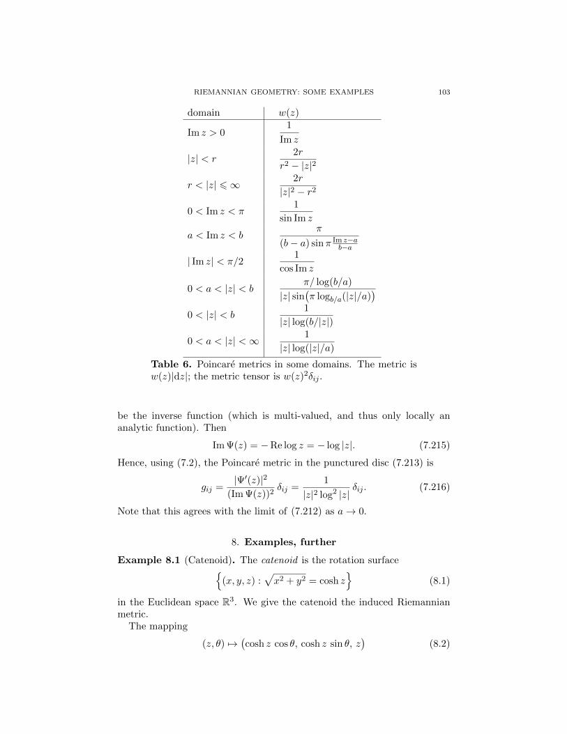
RIEMANNIAN GEOMETRY: SOME EXAMPLES 103
domain w(z)
Im z > 01
Im z
|z| < r2r
r2 − |z|2
r < |z| 6∞ 2r
|z|2 − r2
0 < Im z < π1
sin Im z
a < Im z < bπ
(b− a) sinπ Im z−ab−a
| Im z| < π/21
cos Im z
0 < a < |z| < bπ/ log(b/a)
|z| sin(π logb/a(|z|/a)
)0 < |z| < b
1
|z| log(b/|z|)
0 < a < |z| <∞ 1
|z| log(|z|/a)
Table 6. Poincare metrics in some domains. The metric isw(z)|dz|; the metric tensor is w(z)2δij .
be the inverse function (which is multi-valued, and thus only locally ananalytic function). Then
Im Ψ(z) = −Re log z = − log |z|. (7.215)
Hence, using (7.2), the Poincare metric in the punctured disc (7.213) is
gij =|Ψ′(z)|2
(Im Ψ(z))2δij =
1
|z|2 log2 |z|δij . (7.216)
Note that this agrees with the limit of (7.212) as a→ 0.
8. Examples, further
Example 8.1 (Catenoid). The catenoid is the rotation surface(x, y, z) :
√x2 + y2 = cosh z
(8.1)
in the Euclidean space R3. We give the catenoid the induced Riemannianmetric.
The mapping
(z, θ) 7→(cosh z cos θ, cosh z sin θ, z
)(8.2)
104 SVANTE JANSON
maps the plane R2 onto the catenoid: this map has period 2π in θ and isa diffeomorphism of the cylinder R × (R/2πZ) onto the catenoid. Hence,the restriction to θ ∈ (θ0, θ0 + 2π) yields a coordinate system (covering thecatenoid except for the line θ = θ0). A simple calculation shows that theRiemannian metric in this coordinate system is given by the metric tensor
g11 = sinh2 z + 1 = cosh2 z, g12 = g21 = 0, g22 = cosh2 z, (8.3)
or in matrix form
(gij) =
(cosh2 z 0
0 cosh2 z
). (8.4)
This is a conformal metric of the special type (4.70), with ϕ(z) = log cosh z.The connection coefficients are, by (4.71),
Γ111 = −Γ1
22 = Γ212 = Γ2
21 = tanh z (8.5)
with all other components Γkij = 0.
The curvature tensor is by (4.72)–(4.73) given by
R1212 = −1, (8.6)
which by (3.1)–(3.8) yields all components Rijkl, Rij and R as well as
K =1
2R =
R1212
g211
= − 1
cosh4 z. (8.7)
The catenoid is thus a surface with non-constant negative curvature.
Appendix A. Symmetries of the curvature tensor
We explore the consequences of the symmetries (2.5)–(2.6) and the Bianchiidentity (2.8). (In this section we consider tensors at a single point only. Thesection is thus linear algebra, dealing with tensors over a given n-dimensionalvector space. We could start with any vector space V of finite dimensionand a given non-singular symmetric covariant tensor gij .)
Let R4 be the space of all covariant 4-tensors that satisfy (2.5)–(2.6) and(2.8). Thus the curvature tensor Rijkl ∈ R4.
As another example, for any symmetric tensors Aij and Bij , the definition(1.22) of the Kulkarni–Nomizu product Aij Bkl shows that it satisfies therelations (2.5)–(2.6) and (2.8); i.e., Aij Bkl ∈ R4.
We begin by finding the dimension of R4.It follows from (2.5) that if Rijkl 6= 0, then i 6= j and k 6= l. In particular,
no index occurs more than twice. This leaves three cases.
(i) i, j, k, l are distinct. There are(n4
)sets of four distinct indices in
1, . . . , n. Each such set may be ordered in 4! = 24 different ways,but as said in Section 2, only 2 of these yield linearly independentcomponents Rijkl.
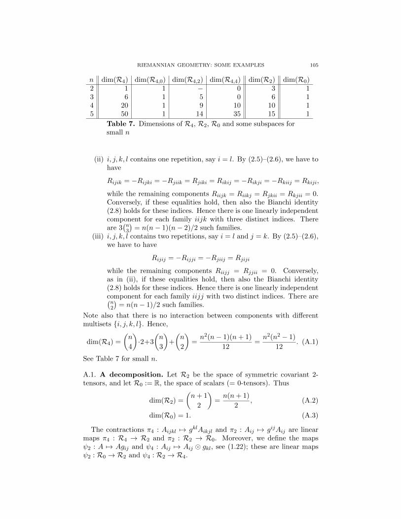
RIEMANNIAN GEOMETRY: SOME EXAMPLES 105
n dim(R4) dim(R4,0) dim(R4,2) dim(R4,4) dim(R2) dim(R0)2 1 1 − 0 3 13 6 1 5 0 6 14 20 1 9 10 10 15 50 1 14 35 15 1
Table 7. Dimensions of R4, R2, R0 and some subspaces forsmall n
(ii) i, j, k, l contains one repetition, say i = l. By (2.5)–(2.6), we have tohave
Rijik = −Rijki = −Rjiik = Rjiki = Rikij = −Rikji = −Rkiij = Rkiji,
while the remaining components Riijk = Riikj = Rjkii = Rkjii = 0.Conversely, if these equalities hold, then also the Bianchi identity(2.8) holds for these indices. Hence there is one linearly independentcomponent for each family iijk with three distinct indices. Thereare 3
(n3
)= n(n− 1)(n− 2)/2 such families.
(iii) i, j, k, l contains two repetitions, say i = l and j = k. By (2.5)–(2.6),we have to have
Rijij = −Rijji = −Rjiij = Rjiji
while the remaining components Riijj = Rjjii = 0. Conversely,as in (ii), if these equalities hold, then also the Bianchi identity(2.8) holds for these indices. Hence there is one linearly independentcomponent for each family iijj with two distinct indices. There are(n2
)= n(n− 1)/2 such families.
Note also that there is no interaction between components with differentmultisets i, j, k, l. Hence,
dim(R4) =
(n
4
)·2+3
(n
3
)+
(n
2
)=n2(n− 1)(n+ 1)
12=n2(n2 − 1)
12. (A.1)
See Table 7 for small n.
A.1. A decomposition. Let R2 be the space of symmetric covariant 2-tensors, and let R0 := R, the space of scalars (= 0-tensors). Thus
dim(R2) =
(n+ 1
2
)=n(n+ 1)
2, (A.2)
dim(R0) = 1. (A.3)
The contractions π4 : Aijkl 7→ gklAikjl and π2 : Aij 7→ gijAij are linearmaps π4 : R4 → R2 and π2 : R2 → R0. Moreover, we define the mapsψ2 : A 7→ Agij and ψ4 : Aij 7→ Aij gkl, see (1.22); these are linear mapsψ2 : R0 → R2 and ψ4 : R2 → R4.

106 SVANTE JANSON
By (1.3), for any A ∈ R0,
π2ψ2(A) = π2(Agij) = gijAgij = nA, (A.4)
i.e., π2ψ2 = nI, where I is the identity map. Hence we have the directdecomposition
R2 = R2,2 ⊕R2,0, (A.5)
where
R2,2 := ker(π2) = the set of traceless tensors in R2, (A.6)
R2,0 := im(ψ2) = rgij : r ∈ R. (A.7)
Explicitly, a tensor Aij ∈ R2 decomposes as
Aij = A(0)ij +A
(2)ij , (A.8)
where, with A := π2(Aij) = gijAij ,
A(0)ij :=
1
nAgij ∈ R2,0, (A.9)
A(2)ij := Aij −A(0)
ij = Aij −1
nAgij ∈ R2,2. (A.10)
Moreover, with the inner product on R2
〈Aij , Bij〉 := AijBij = gikgjlAijBkl, (A.11)
it is easily seen that ψ∗2 = π2, and thus R2,0 ⊥ R2,2, so the decomposition(A.5) is orthogonal.
We have
dim(R2,2) = dim(R2)− 1 =n(n+ 1)
2− 1 =
(n− 1)(n+ 2)
2. (A.12)
Similarly, we compute for Aij ∈ R2, with A := gijAij ,
π4ψ4(Aij)) = π4
(Aij gkl
)= gkl
(Aik gjl
)= gkl
(Aijgkl +Aklgij −Ailgkj −Akjgil
)= nAij +Agij −Aij −Aij =
((n− 2) + ψ2π2)(Aij)
). (A.13)
Hence, using (A.4),
π4ψ4 =
(n− 2)I on R2,2,
(n− 2 + n)I = 2(n− 1)I on R2,0.(A.14)
A.1.1. The case n > 3. Suppose now n > 3. Then (A.14) shows that π4ψ4
is an isomorphism of R2 = R2,2 ⊕ R2,0 onto itself; hence π4 : R4 → R2 issurjective, ψ4 : R2 → R4 is injective and
R4 = ker(π4)⊕ im(ψ4) = ker(π4)⊕ψ4(R2) = ker(π4)⊕ψ4(R2,2)⊕ψ4(R2,0).(A.15)
We write this as
R4 = R4,0 ⊕R4,2 ⊕R4,4 (A.16)

RIEMANNIAN GEOMETRY: SOME EXAMPLES 107
with
R4,0 := ψ4(R2,0) = ψ4(ψ2(R0)) = rgij gkl : r ∈ R, (A.17)
R4,2 := ψ4(R2,2) = Aij gkl : Aij ∈ R2 and gijAij = 0, (A.18)
R4,4 := ker(π4). (A.19)
Explicitly, if Aijkl ∈ R4, it has a unique decomposition
Aijkl = A(0)ijkl +A
(2)ijkl +A
(4)ijkl (A.20)
with A(m)ijkl ∈ R4,m, viz., using the contractions Aij := π4(Aijkl) = gklAikjl
and A := π2(π4(Aijkl)) = gijAij = gijgklAikjl,
A(0)ijkl =
1
2n(n− 1)Agij gkl, (A.21)
A(2)ijkl =
1
n− 2
(Aij −
1
nAgij
) gkl, (A.22)
A(4)ijkl = Aijkl −A
(0)ijkl −A
(2)ijkl
= Aijkl −1
n− 2Aij gkl +
1
2(n− 1)(n− 2)Agij gkl. (A.23)
In particular, for the Riemann curvature tensor, this gives the decomposition
(2.15), where the Weyl tensor Wijkl := R(4)ijkl.
With the natural inner product on R4,
〈Aijkl, Bijkl〉 := AijklBijkl, (A.24)
we have, similarly to R2 treated above, using the assumption that Aijkl ∈R4, and thus satisfies (2.5)–(2.6),
〈ψ∗4(Aijkl), Bij〉 = 〈Aijkl, Bij gkl〉= 〈Aijkl, Bikgjl +Bjlgik −Bilgjk −Bjkgil〉
= 4〈Aijkl, Bikgjl〉 = 4AijklBikgjl
= 4〈π4(Aijkl), Bij〉, (A.25)
which shows that ψ∗4 = 4π4 and thus π∗4 = 14ψ4. This, together with (A.14),
shows that the decomposition (A.16) is orthogonal.We note also that
dim(R4,4) = dim(R4)− dim(R2) =n2(n+ 1)(n− 1)
12− n(n+ 1)
2
=n(n+ 1)(n+ 2)(n− 3)
12. (A.26)
108 SVANTE JANSON
A.1.2. The case n = 3. In the special case n = 3, (A.26) shows that
dim(R4,4) = 0, so A(4)ijkl = 0 for every tensor Aijkl ∈ R4, and (A.20) takes
the simpler form
Aijkl = A(0)ijkl +A
(2)ijkl =
1
12Agij gkl +
(Aij −
1
3Agij
) gkl
=(Aij −
1
4Agij
) gkl. (A.27)
A.1.3. The case n = 2. When n = 2, (A.14) shows that π4ψ4 vanisheson R2,2 but is an isomorphism on R2,0
∼= R0. In fact, (A.1) shows thatdim(R4) = 1 = dim(R2,0); thus ψ4 restricts to an isomorphism of R2,0 ontoR4 and π4 maps R4 onto R2,0 and is an isomorphism R4 → R2,0. Moreover,π4ψ4 = 2I on R2,0 and ψ4π4 = 2I on R4.
Consequently, for every Aijkl ∈ R4, with the contractions Aij and A asabove, using also (A.9),
Aijkl = 12Aij gkl = 1
4Agij gkl. (A.28)
In other words, we still have the decomposition (A.20) even when n = 2, with
A(0)ijkl given by (A.21) but A
(2)ijkl = A
(4)ijkl := 0. In fact, R4,4 = ker(π4) = 0.
Note that the contraction Aij = π4(Aijkl) ∈ R2,0 for every Aijkl ∈ R4, i.e.
Aij = 12Agij , (A.29)
unlike the case n > 3 where, as we saw above, Aij can be any symmetrictensor.
Appendix B. Curves with constant curvature
Consider a 2-dimensional manifold M . By Section 1.5, a curve γ (withγ 6= 0) has constant curvature if and only if it can be reparametrized (byarc length) to have constant velocity 1 and an acceleration vector that hasconstant length and is orthogonal to the velocity vector. For a given non-zero curvature, this gives two choices for the acceleration vector (since weassume n = 2), but for a smooth curve, the acceleration is (locally) always onthe same side of the velocity vector by continuity (left or right, as definedby the coordinates); hence the acceleration is determined by the velocityvector and the curvature. This gives a (non-linear) second order differentialequation for γ(t), which has a unique maximal solution γ : (−a, b)→M foreach set of initial values, ı.e., for each initial point γ(0), each unit tangentvector γ(0) and each curvature κ ∈ [0,∞), with an initial direction of thecurvature unless it is 0. (The case of curvature 0 yields the geodesics.)
We consider such curves in convenient models of 2-dimensional manifoldswith constant curvature.
B.1. Circles. A circle with radius r is the set of points of distance r > 0from some point x0 (the centre).

RIEMANNIAN GEOMETRY: SOME EXAMPLES 109
B.1.1. Plane, zero curvature. In the standard Euclidean plane with curva-ture 0, we take the centre as 0 and can parametrize the circle as
γ(t) = (r cos t, r sin t). (B.1)
If we identify R2 and the complex plane C, we can write this more simplyas γ(t) = reit. The radius is r, the velocity vector is
γ(t) = (−r sin t, r cos t) = ireit (B.2)
with length r, and the acceleration is
γ(t) = (−r cos t,−r sin t) = −reit (B.3)
with length r (orthogonal to γ since the velocity is constant). Note that wehave chosen a parametrization with constant velocity, but not necessarilyvelocity 1 (i.e., parametrization by arc length). The curvature is by (1.32)
κ =r
r2=
1
r. (B.4)
The curvature vector is directed towards the centre of the circle.We see that the curvature κ = 1/r ∈ (0,∞), and that every positive
curvature is obtained by some circle.The circle is a closed curve which really is given by (B.1) for t ∈ [0, 2π);
hence by (B.2) its length is, as has been well-known since antiquity,
` = 2πr. (B.5)
Equally well-known is that the area of a circle of radius r is
A = πr2, (B.6)
which can be verified by integrating the measure (1.6), which now is Lebesguemeasure, for |x| 6 r.
Note that the total (geodesic) curvature of the circle (measured inwards)is ∫
γκ = `κ = 2π, (B.7)
for every circle.
We have here used Euclidean coordinates. As an alternative, we may in-stead use polar coordinates, see Example 5.2. Then the circle above (exceptfor a point) can be parametrized as
γ(t) = (r, t), 0 < t < 2π, (B.8)
with velocity vector
γ(t) = (0, 1), (B.9)
with length r by (5.2). Furthermore,
γ(t) = 0, (B.10)
and thus the acceleration is by (1.29), (B.9) and (5.4)–(5.5),
D2t γ(t) = (Γ1
22,Γ222) = (−r, 0), (B.11)

110 SVANTE JANSON
with length r by (5.2), which again yields the formula (B.4) for the curvature.(See also the more general (4.29)–(4.32).) We also immediately obtain (B.5)and (B.6) for the length and area, using the invariant measure (5.6) for thelatter.
B.1.2. Sphere, positive curvature. Consider the sphere S2ρ of radius ρ in (6.1),
which has constant curvature K = ρ−2 > 0 by (6.11). Note that the maxi-mum distance in S2
ρ (i.e., its diameter as a metric space) is πρ, and thus thereare circles only with radii 0 < r < πρ. (The case r = πρ is degenerate, sinceit would give a single point only and not a curve.) Note also that a circleof radius r and centre x0 is the same as a circle of radius πρ− r and centre−x0, the antipode. Hence it suffices to consider the case 0 < r 6 πρ/2,although we allow larger r too below unless we indicate otherwise.
The circles with radius r = πρ/2 are the geodesics in S2ρ.
All circles of the same radius are congruent by rotations of the sphere,so it suffices to consider one of them. We may also use any convenientcoordinate system. As an illustration of the calculations, we consider as inSection B.1 two alternatives.
We first use the stereographic coordinates in Example 6.1. We considerthe curve
γ(t) = (a cos t, a sin t), t ∈ R, (B.12)
with a > 0. This is by (6.22) a circle with centre 0 and radius r ∈ (0, πρ)given by
tan( r
2ρ
)=a
ρ. (B.13)
We have γ(t) = (−a sin t, a cos t) and thus, using (6.7),
‖γ(t)‖2 =4a2
(1 + a2/ρ2)2. (B.14)
Furthermore, γ(t) = (−a cos t,−a sin t) = −γ(t), and it follows from (1.29)and (6.10) that (by rotational symmetry it suffices to consider t = 0)
D2t γ
k = γk + Γkij γiγj = −γk +
2a2
ρ2 + a2γk = −ρ
2 − a2
ρ2 + a2γk, (B.15)
and thus
‖D2t γ(t)‖ =
|ρ2 − a2|ρ2 + a2
‖γ(t)‖ =|ρ2 − a2|ρ2 + a2
2a
1 + a2/ρ2. (B.16)
Hence (1.32) yields, noting that the velocity is constant by (B.14) and thusthe acceleration D2
t γ(t) ⊥ γ(t) as seen in (B.15), and using (B.13),
κ =‖D2
t γ(t)‖‖γ(t)‖2
=|1− a2/ρ2|
2a=|1− tan2(r/2ρ)|
2ρ tan(r/2ρ)=
1
ρ | tan(r/ρ)|. (B.17)
If we consider only r 6 πρ/2, we can write this as
κ =cot(r/ρ)
ρ, 0 < r 6 πρ/2. (B.18)

RIEMANNIAN GEOMETRY: SOME EXAMPLES 111
Note that for r = πρ/2, the curvature vanishes and the circle is a geodesic,as said above.
The absolute value in (B.17) is explained by the fact that we have definedthe curvature κ as a non-negative scalar. If we instead consider the curvaturevector (1.34), we can say that, for all r ∈ (0, πρ), the curvature vector iscot(r/ρ)/ρ directed towards the centre of the circle, i.e., (B.18) holds forall r if we measure the curvature in the direction towards the centre. (See(B.15) and note that this description yields the same vector if we considerthe circle as a circle with radius πρ− r about the antipodal centre.)
For 0 < r < πρ/2, the curvature vector is directed towards the centreof the circle; the curvature κ = cot(r/ρ)/ρ ∈ (0,∞), and every positivecurvature is obtained by some circle with radius r < πρ/2.
The circle is a closed curve which really is given by (B.12) for t ∈ [0, 2π);hence its length is, by (B.14) and (B.13),
` = 2π2a
1 + a2/ρ2= 4πρ
tan(r/2ρ)
1 + tan2(r/2ρ)= 2πρ sin
r
ρ, (B.19)
as is also seen by elementary geometry. The area of a circle of radius r is,by integrating the measure (6.15) for |x| 6 a or by elementary geometry,
A = 4πρ2 sin2 r
2ρ= 2πρ2
(1− cos
r
ρ
). (B.20)
Note that the total (geodesic) curvature of the circle (measured inwards; wehere allow κ < 0) is ∫
γκ = `κ = 2π cos(r/ρ) (B.21)
while the total curvature of the interior is, using (6.11),∫K dµ = KA =
1
ρ2A = 2π
(1− cos
r
ρ
). (B.22)
Hence ∫γκ+
∫K dµ = `κ+KA = 2π (B.23)
for every circle, an example of the Gauss–Bonnet theorem.
As an alternative (and partly simpler) calculation, we consider polar co-ordinates on a sphere, see Example 6.7; for simplicity we consider as inExample 6.7 only the unit sphere with ρ = 1. Then as in (B.8), the circleabove with centre 0 and radius r can be parametrized as
γ(t) = (r, t), 0 < t < 2π, (B.24)
with velocity vector
γ(t) = (0, 1), (B.25)
with length sin r by (6.74). Furthermore,
γ(t) = 0, (B.26)
112 SVANTE JANSON
and thus the acceleration is by (1.29), (B.25) and (6.76)–(6.77), in accor-dance with the more general (4.29),
D2t γ(t) = (Γ1
22,Γ222) = (− sin r cos r, 0), (B.27)
with length
‖D2t γ(t)‖ = | sin r cos r| (B.28)
by (6.74). Hence the curvature (1.32) is, see also (4.32),
κ =‖D2
t γ(t)‖‖γ(t)‖2
=| sin r cos r|
sin2 r= | cot r| (B.29)
in accordance with (B.17)–(B.18) (with ρ = 1). Furthermore, we see imme-diately from (6.74) that the length of the circle is
` = 2π sin r (B.30)
as in (B.19); similarly, the area is, using the invariant measure (6.78),
A =
∫ r
ϕ=0
∫ 2π
θ=0sinϕdϕdθ = 2π
(1− cos r
)(B.31)
as in (B.20).
Finally, consider again a general sphere with radius ρ. If ` is a geodesicand 0 < d < πρ/2, then the set of points of distance d to ` form two circles,one in each half-sphere bounded by `, both having radius πρ/2−d and thusby (B.18) curvature
κ =cot(π/2− d/ρ)
ρ=
tan(d/ρ)
ρ. (B.32)
(If ` is the equator, these circles are parallels, where the latitude is constant.)Conversely, every circle is the set of points of distance d = ρ arctan(ρκ) tosome geodesic `, and further lying in one of the two half-spheres defined by`.
B.1.3. Hyperbolic plane, negative curvature. Consider the hyperbolic plane,which can be represented by, for example, the Poincare half-plane H2 inExample 7.1 or the Poincare disc D2 in Example 7.3. The (sectional) curva-ture is K = −1, see (7.11) and (7.26). (We consider for simplicity only thiscase. Any other constant negative curvature can be obtained by scaling themetric, see Example 7.4.)
All circles of the same radius are congruent by isometries of the hyperbolicplane, since the isometry group is transitive, so it suffices to consider oneof them. We choose to use the model D2 in Example 7.3 and consider thecurve
γ(t) = (a cos t, a sin t), t ∈ R, (B.33)
with 0 < a < 1. This is by (7.37) a circle with centre 0 and radius r ∈ (0,∞)given by
tanhr
2= a. (B.34)
RIEMANNIAN GEOMETRY: SOME EXAMPLES 113
We have γ(t) = (−a sin t, a cos t) and thus, using (7.23),
‖γ(t)‖2 =4a2
(1− a2)2. (B.35)
Furthermore, γ(t) = (−a cos t,−a sin t) = −γ(t), and it follows from (1.29)and (7.25) that (by rotational symmetry it suffices to consider t = 0)
D2t γ
k = γk + Γkij γiγj = −γk − 2a2
1− a2γk = −1 + a2
1− a2γk, (B.36)
and thus
‖D2t γ(t)‖ =
1 + a2
1− a2‖γ(t)‖ =
2a(1 + a2)
(1− a2)2. (B.37)
Hence (1.32) yields, noting that the velocity is constant by (B.35) and thusthe acceleration D2
t γ(t) ⊥ γ(t) as seen in (B.36), and using (B.34),
κ =‖D2
t γ(t)‖‖γ(t)‖2
=1 + a2
2a=
1 + tanh2(r/2)
2 tanh(r/2)=
1
tanh r= coth r. (B.38)
The curvature vector is (as in the Euclidean case, and for small circles on asphere) directed towards the centre of the circle, see (B.36).
Note that the curvature κ = coth r ∈ (1,∞), and that every curvature > 1is obtained by some circle; however hyperbolic circles cannot have curvature6 1. Hence (unlike the Euclidean and spherical cases), there are also othercurves than circles with constant curvature in the hyperbolic plane. Weconsider these in the next two subsections.
A hyperbolic circle (B.33) is a closed curve and its length is, by (B.35)and (B.34),
` = 2π2a
1− a2= 4π
tanh(r/2)
1− tanh2(r/2)= 2π sinh r. (B.39)
The area of a circle of radius r is, by integrating the measure (7.30) for|x| 6 a,
A = 4πa2
1− a2= 4π sinh2 r
2= 2π(cosh r − 1). (B.40)
Note that the total (geodesic) curvature of the circle (measured inwards) is∫γκ = `κ = 2π cosh r (B.41)
while the total curvature of the interior is, using (7.26),∫K dµ = KA = −A = 2π(1− cosh r). (B.42)
Hence ∫γκ+
∫K dµ = `κ+KA = 2π (B.43)
for every hyperbolic circle, another example of the Gauss–Bonnet theorem.

114 SVANTE JANSON
Again, the calculations are simpler if we instead use polar coordinates,see Example 7.8. Then as in (B.8) and (B.24), the circle with centre 0 andradius r can be parametrized as
γ(t) = (r, t), 0 < t < 2π, (B.44)
with velocity vectorγ(t) = (0, 1), (B.45)
with length sinh r by (7.105). Furthermore,
γ(t) = 0, (B.46)
and thus the acceleration is by (1.29), (B.45) and (7.107)–(7.108), in accor-dance with the more general (4.29),
D2t γ(t) = (Γ1
22,Γ222) = (− sinh r cosh r, 0), (B.47)
with length, by (7.105),
‖D2t γ(t)‖ = sinh r cosh r (B.48)
Hence the curvature (1.32) is, see also (4.32),
κ =‖D2
t γ(t)‖‖γ(t)‖2
=sinh r cosh r
sinh2 r= coth r (B.49)
in accordance with (B.38). Furthermore, we see from (7.105) immediatelythat the length of the circle is
` = 2π sinh r (B.50)
as in (B.39); similarly, the area is, using the invariant measure (7.109),
A =
∫ r
s=0
∫ 2π
θ=0sinh s ds dθ = 2π(cosh r − 1) (B.51)
as in (B.40).See also the equal-area representation Example 7.11, in particular (7.127).
B.2. Horocycles in the hyperbolic plane. We have seen in Section B.1that in the hyperbolic plane, curves with constant curvature 6 1 are notcircles. We describe these curves in this and the following subsections; inthis subsection we discuss the curves of constant curvature κ = 1, which arecalled horocycles.
Note that through every point, there is a unique (undirected) horocyclewith a given curvature vector ~κ of length 1. In other words, there are twohorocycles (with curvature vectors in opposite directions) through each pointwith a given tangent.
All horocycles are congruent by isometries of the hyperbolic plane, sincethe isometry group is transitive and the group of isometries fixing a givenpoint is transitive on the tangent vectors there; hence it suffices to considerone horocycle.
We choose the model H2 in Example 7.1 and consider the curve
γ(t) = (t, 1), t ∈ R, (B.52)

RIEMANNIAN GEOMETRY: SOME EXAMPLES 115
i.e., the Euclidean horizontal line y = 1. (We could consider choose y = y0
for any y0 > 0, but we need only one example so we take the simplest.)We have γ(t) = (1, 0) and thus by (7.2)
‖γ(t)‖2 = 1. (B.53)
Furthermore, γ(t) = 0 and it follows from (1.29) and (7.4) that
D2t γ
k = γk + Γkij γiγj = Γk11 = δk2, (B.54)
i.e., D2t γ(t) = (0, 1), and thus
‖D2t γ(t)‖ = 1. (B.55)
Hence (1.32) yields, noting that the velocity is constant and thus the accel-eration D2
t γ(t) ⊥ γ(t), as also seen directly in (B.54),
κ = 1, (B.56)
verifying that the curve (B.52) indeed is a horocycle. The curvature vectoris directed upwards.
The orientation-preserving isometries of the Poincare half-plane H2 arethe Mobius transformations that preserve H2, i.e., the mappings z 7→ az+b
cz+d
with a, b, c, d real and ad − bc > 0. The horocycle (B.52) is a circle in theRiemann sphere S2 = C ∪ ∞ with exactly one point, viz. ∞, in commonwith the boundary ∂H2. It follows that the horocycles in H2 are preciselythe circles in S2 with one point on ∂H2 and the rest in H2, i.e., the Euclideanhorizontal lines y = y0 with y0 > 0 (including (B.52)) and the Euclideancircles in the upper half plane H2 that are tangent to the real axis. (Thecurvature vector is directed upwards in the first case and inwards the circlein the second case. The curvature vector lies on a geodesic that ends at thepoint where the horocycle meets the boundary ∂H2.)
Since H2 and the Poincare disc D2 are isometric by a Mobius transfor-mation, it follows also that the horocycles in D2 are the Euclidean circlesthat are tangent to the unit circle ∂D (on the inside); the curvature vector isdirected inwards this circle. (Again, the curvature vector lies on a geodesicthat ends at the point where the horocycle meets the boundary ∂D2.)
A horocycle has infinite length, and it separates the hyperbolic planeinto two parts, both having infinite area. (This is seen by considering thehorocycle (B.52).)
B.3. Hypercycles in the hyperbolic plane. The curves of constant cur-vature κ < 1 in the hyperbolic plane are called hypercycles.
Note that through every point, there is a unique (undirected) hypercyclewith a given curvature vector ~κ of length < 1. In other words, there aretwo hypercycles (with curvature vectors in opposite directions) through eachpoint with a given tangent direction and a given curvature κ < 1.
All hypercycles with the same curvature are congruent by isometries ofthe hyperbolic plane; hence it suffices to consider one example for eachcurvature κ < 1.

116 SVANTE JANSON
We choose the model H2 in Example 7.1 and consider the curve
γ(t) = (αet, et), t ∈ R, (B.57)
with 0 < α <∞, i.e., a Euclidean line through the origin. (The case α = 0yields a geodesic, and the case α < 0 is equivalent to α > 0 by reflection inthe y-axis.)
We have γ(t) = γ(t) and thus by (7.2)
‖γ(t)‖2 = e−2t(α2e2t + e2t) = α2 + 1. (B.58)
Furthermore, γ(t) = γ(t) and it follows from (1.29) and (7.4) that
D2t γ
k = γk + Γkij γiγj = γk(t)− e−t
(2etγk(t)− δk2(1 + α2)e2t
)= −γk(t) + δk2(1 + α2)γ2(t), (B.59)
i.e.,
D2t γ = (−α, α2)et, (B.60)
and thus, by (7.2),
‖D2t γ(t)‖2 = α2 + α4. (B.61)
Hence (1.32) yields, noting that the velocity is constant and thus the accel-eration D2
t γ(t) ⊥ γ(t), as also seen directly in (B.61),
κ =α√
1 + α2
1 + α2=
α√1 + α2
. (B.62)
verifying that the curve (B.57) indeed is a hypercycle. The curvature vectoris directed towards the y-axis.
Note that there is a unique α > 0 satisfying (B.62) for every given κ ∈(0, 1); hence there is a unique hypercycle (B.57) for every curvature κ < 1.
The hypercycles are thus the curves in the hyperbolic plane that arecongruent to one of the curves (B.57). Since the isometries of H2 and D2
are given by Mobius mappings and reflections, it follows that in both H2
and D2, the hypercycles are the Euclidean circles and lines that intersectthe boundary in two different points, but not orthogonally. (The circlesand lines that are orthogonal to the boundary are congruent to (B.57) withα = 0, and are thus geodesics.) The angle of intersection with the boundaryis invariant under isometries; hence a Euclidean line or circle intersectingthe boundary ∂H2 or ∂D2 at an angle θ ∈ (0, π/2] is congruent to (B.57)with α = cot θ, and is thus by (B.62) a hypercycle with curvature
κ = cos θ, (B.63)
unless θ = π/2 in which case the curve is a geodesic. (The relation (B.63)holds in the latter case too, with κ = 0.) Conversely, every hypercycle inH2 or D2 is thus a Euclidean line or circle intersecting the boundary intwo points, at each point with an angle θ ∈ (0, π/2) satisfying (B.63), i.e.,θ = arccosκ.
RIEMANNIAN GEOMETRY: SOME EXAMPLES 117
Considering again H2, the y-axis (0, u) is, as said above, a geodesic.The distance d from a point (x, y) to the y-axis is, by (7.12), given by
cosh d = infu>0
d((x, y), (0, u)
)= inf
u>0
(1 +
x2 + (y − u)2
2yu
)= inf
u>0
x2 + y2 + u2
2yu. (B.64)
This infimum is attained for u =√x2 + y2, which gives
cosh d =
√x2 + y2
y(B.65)
and thus
sinh d =|x|y. (B.66)
(This can also be seen geometrically; the geodesics orthogonal to the y-axisare the Euclidean circles with centre 0, so the one passing through (x, y)
has Euclidean radius√x2 + y2 and intersects the y-axis in (0,
√x2 + y2),
see (7.20).) Hence, the points on the hypercycle (B.57) all have the samedistance d to the y-axis, with sinh d = α. By (B.62), the curvature of thehypercycle is
κ =sinh d√
1 + sinh2 d= tanh d. (B.67)
Applying isometries, we see that for any geodesic ` in the hyperbolicplane, and any d > 0, the points of distance d to ` form two hypercycles,one in each (hyperbolic) half-plane bounded by `, both having curvatureκ = tanh d given by (B.67). (Cf. (B.18) in the spherical case.) Conversely,every hypercycle is the set of points of distance d = arctanhκ to somegeodesic `, and further lying in one of the two half-planes defined by `.Note that the hypercycle and the geodesic have the same endpoints in theboundary (line at infinity) of the hyperbolic plane, which defines the geodesiccorresponding to a given hypercycle.
Note also that a hypercycle that makes an angle θ ∈ (0, π/2) with theboundary (line at infinity) has curvature κ = cos θ by (B.63), and thus(B.67) shows that the distance d to the corresponding geodesic satisfies
tanh d = cos θ (B.68)
and hence also
cosh d =1
sin θ, (B.69)
sinh d = cot θ. (B.70)

118 SVANTE JANSON
B.4. Summary for the hyperbolic plane. For both the Poincare half-plane H2 (Example 7.1) and the Poincare disc D2 (Example 7.3), we haveseen that the circles, horocycles, hypercycles and geodesics together are allEuclidean lines and circles that intersect the half-plane or disc; moreover,they can be distinguished as follows:
(i) Circles do not intersect the boundary (line at infinity); they areEuclidean circles completely included in H2 or D2.
(ii) Horocycles intersect the boundary in exactly one point; they aretangent to the boundary and lie inside H2 or D2 except for thetangent point.
(iii) Hypercycles intersect the boundary in two distinct points, at anangle θ ∈ (0, π/2).
(iv) Geodesics intersect the boundary in two distinct points, at an angleθ = π/2.
Note that horocycles can be seen as limiting cases of circles (letting theradius r → ∞), and also of hypercycles (letting the angle θ at the line ofinfinity tend to 0, or equivalently letting the distance d to a geodesic tendto ∞). In both cases, the curvatures given by (B.38) and (B.63) or (B.67)tend to 1, the value for horocycles.
Appendix C. Curves in the complex plane
We consider here a (smooth) curve γ(t) in the complex plane C, with theusual Euclidean metric. We assume γ(t) 6= 0. Furthermore, we considerthe curvature κ in (1.32) with sign, as explained in Remark 1.2. Thus, see(1.34), ~κ is a positive number times iκγ, and it follows from (1.35) that
~κ =iκγ
‖γ‖=
iκγ
|γ|. (C.1)
Consequently,
κ =~κ|γ|iγ
=~κ|γ|iγ
=PN γ
iγ|γ|= Im
γ
γ|γ|. (C.2)
As a consequence, using |γ| = (γγ)1/2,
d
dtκ(t) = Im
d
dt
( γγ|γ|−1
)= Im
(d
dt
( γγ
)|γ|−1 − 1
2
γ
γ|γ|−3
(γγ + γγ
))=
1
|γ|Im
(d
dt
( γγ
)− 1
2
(γ
γ
)2)
(C.3)
Define, for a thrice differentiable function f(x) of a real or complex vari-able, the Schwarzian derivative S(f) by
S(f)(x) :=
(f ′′
f ′
)′− 1
2
(f ′′
f ′
)2
=f ′′′
f ′− 3
2
(f ′′
f ′
)2
. (C.4)

RIEMANNIAN GEOMETRY: SOME EXAMPLES 119
Then (C.3) can be written
d
dtκ(t) =
1
|γ(t)|ImS(γ)(t). (C.5)
A standard calculation yields, for an analytic function g,
S(g f)(x) = S(g)(f(x)) · f ′(x)2 + S(f)(x). (C.6)
Hence, (C.5) implies that if κ(t) is the (signed) curvature of g γ(t), then
d
dtκ(t) =
1
|g′(γ(t))| |γ(t)|Im(S(g)(γ(t)) · γ(t)2
)+
1
|g′(γ(t))|d
dtκ(t). (C.7)
Remark C.1. If γ(t) is parametrized by arc-length, so |γ(t)| = 1, and κ isreparametrized as κ(s) where s is its arc-length, then (C.7) takes the simplerform
|g′(γ(t))|2 d
dsκ(s) = Im
(S(g)(γ(t)) · γ(t)2
)+
d
dtκ(t). (C.8)
Remark C.2. It is well-known that S(g) = 0 if and only if g is a Mobiustransformation, i.e., a fractional linear map g(z) = (az + b)/(cz + d) (witha, b, c, d ∈ C and ad − bc 6= 0 so that g is not constant), cf. (6.36). Hence,(C.6) implies that if g is a Mobius transformation, then S(g f) = S(f)for any f . Conversely, it is known that if S(h) = S(f) for two analyticfunctions, then h = g f for some Mobius transformation g.
If γ is a curve with constant curvature, we see by (C.7) that g(γ) also isa curve with constant curvature if and only if
S(g)(γ(t)) · γ(t)2 ∈ R. (C.9)
Example C.3. Let g be an analytic function g, defined in some domainΩ ⊆ C. It follows from (C.9) that g maps all (parts of) circles and lines to(parts of) circles and lines if and only if g′ 6= 0 and S(g) = 0 in Ω, which byRemark C.2 occurs if and only if g is a Mobius transformation.
Example C.4. Let g be an analytic function g, defined in some domainΩ ⊆ C. It follows from (C.9) that the following are equivalent:
(i) g maps all horizontal lines to (parts of) circles and lines.(ii) g maps all vertical lines to (parts of) circles and lines.(iii) S(g) is real.(iv) S(g) = a for some real constant a.
Since the exponential function f(z) = ebz (with a complex constant b 6= 0)by a simple calculation has S(f) = −1
2b2, it follows by Remark C.2 that
these properties are further equivalent to
(v) g(z) has one of the forms
h(z), (C.10)
h(ecz), c > 0, (C.11)
h(eicz), c > 0, (C.12)
for a Mobius transformation h.
120 SVANTE JANSON
Remark C.5. Some alternative formulas for the Schwarzian derivative are
S(f)(x) = −2√f ′(
1√f ′
)′′(C.13)
= 6∂2
∂x∂y
(f(x)− f(y)
x− y
)∣∣∣∣y=x
(C.14)
= 6
(f ′(x)f ′(y)
(f(x)− f(y))2− 1
(x− y)2
)∣∣∣∣y=x
. (C.15)
Appendix D. Geodesics as straight lines
We prove the following result, stated in Section 1.6, characterizing Rie-mannian metrics such that the geodesics are (parts of) straight lines (possi-bly traversed with γ non-constant).
Theorem D.1. Geodesics are straight lines in a coordinate system if andonly if the connection has the special form
Γkij = δki aj + δkj ai (1.37)
for some functions ai.
Proof. We have already shown in Section 1.6 that (1.37) implies that γ isparallel to γ for a geodesic γ, which thus is a straight line.
Conversely, suppose that every geodesic is a straight line. If γ is a geo-desic, then both γ and γ are directed along the line formed by γ, and arethus parallel. At any point x, we may choose any non-zero tangent vector(ti)
n1 and find a geodesic γ with γ(0) = x and γi(0) = ti. By (1.36), then
γi(0) = −Γijktjtk. Consequently, for any choice of (ti)n1 , there exists c such
thatΓijktjtk = cti. (D.1)
Choosing first t` = δi`, we see that
Γijj = 0, i 6= j. (D.2)
Similarly, choosing t` = δi` + δj`, with i 6= j, we see, using (D.2), that
Γkij = 0, k 6= i, j. (D.3)
Next, fixing any two distinct indices i and j and taking ti, tj 6= 0 but tk = 0for k 6= i, j, we find by (D.1), using (D.2)
Γiiit2i + 2Γiijtitj = cti (D.4)
Γjjjt2j + 2Γjijtitj = ctj (D.5)
(with no implicit summation) and thus
Γiiiti + 2Γiijtj = c = Γjjjtj + 2Γjijti. (D.6)
Since ti and tj are arbitrary non-zero, this yields
Γiii = 2Γjij . (D.7)
RIEMANNIAN GEOMETRY: SOME EXAMPLES 121
This is valid for all i 6= j, which shows that (1.37) holds with ai := 12Γiii
when i 6= j and k ∈ i, j; it is furthermore trivially true when i = j = k,and the case k /∈ i, j follows by (D.2)–(D.3).
Appendix E. A matrix lemma
Lemma E.1. Let A = (aij)ni,j=1 be an n× n-matrix of the special form
aij = δij + uivj , i, j = 1, . . . , n, (E.1)
for two vectors u = (ui)n1 and v = (vi)
n1 . Then the determinant of A is
|A| = 1 + 〈u, v〉 = 1 +n∑i=1
uivi, (E.2)
and if |A| 6= 0, then the inverse is
A−1 =(δij −
uivj1 + 〈u, v〉
)ni,j=1
=(δij −
uivj|A|
)ni,j=1
. (E.3)
Proof. The determinant (E.2) may be calculated in several ways. For ex-ample, suppose that u1 6= 0, and subtract ui/u1 times row 1 from row i foreach i = 2, . . . , n; this gives for each i > 2 a new row with elements
δij + uivj −uiu1
(δ1j + u1vj
)= δij −
uiu1δ1j ; (E.4)
note that only (at most) two elements are non-zero, the first and the one onthe diagonal. Next, subtract u1vi times the new row i from the first row,for each i > 2. This gives a new first row with elements
δ1j + u1vj −n∑i=2
u1vi
(δij −
uiu1δ1j
), (E.5)
which vanishes for j > 1 and equals 1 +∑n
i=1 uivi for j = 1. Hence wehave reduced the matrix A to a lower triangular matrix (with the samedeterminant) with one diagonal element 1 + 〈u, v〉 and all other diagonalelements 1; hence (E.2) follows. The case u1 = 0 follows by continuity.
Next, let λ := 〈u, v〉 and B := A− I = (uivj). Then B2 = λB, and thus
(I +B)((1 + λ)I −B) = (1 + λ)I + (1 + λ− 1)B −B2 = (1 + λ)I, (E.6)
and (E.3) follows by dividing by 1 + λ, provided this is non-zero.
References
[1] Explanatory Supplement to the Astronomical Almanac. P.K. Seidel-mann ed., University Science books, Sausalito, CA, 1992.
[2] Shiing-Shen Chern, An elementary proof of the existence of isothermalparameters on a surface, Proc. Amer. Math. Soc. 6 (1955), no. 5, 771–782.
[3] E. Cotton, Sur les varietes a trois dimensions. Annales de la faculte dessciences de Toulouse, Ser. 2, 1 (1899), no. 4, 385–438.
122 SVANTE JANSON
[4] Manfredo Perdigao do Carmo, Riemannian Geometry. Birkhauser,Boston, 1992.
[5] Philip Hartman and Aurel Wintner. On uniform Dini conditions in thetheory of linear partial differential equations of elliptic type. AmericanJournal of Mathematics 77 (1955), no. 2, 329–354.
[6] Udo Hertrich-Jeromin, Introduction to Mobius Differential Geometry.London Mathematical Society Lecture Note Series 300, CambridgeUniv. Press, 2003.
[7] Birger Iversen, Hyperbolic Geometry, Cambridge Univ. Press, 1992.[8] Svante Janson, Euclidean, spherical and hyperbolic trigonometry.
Notes, 2015. http://www.math.uu.se/~svante/papers/sjN16.pdf[9] A. Korn, Zwei Anwendungen der Methode der sukzessiven
Annaherungen, Schwarz Festschrift, Berlin (1914), pp. 215–229.[10] Dmitri Krioukov, Fragkiskos Papadopoulos, Maksim Kitsak, Amin Vah-
dat, Marian Boguna, Hyperbolic geometry of complex networks. Phys.Rev. E (3) 82 (2010), no. 3, 036106.
[11] Joseph-Louis Lagrange, Sur la construction des Cartes geographiques.Noveaux Memoires de l’Academie royale des Sciences et Belles-Lettresde Berlin, 1779. Reprinted in Oeuvres de Lagrange, vol. 4, pp. 637–692,Gauthier-Villars, Paris, 1867–1892.
[12] L. Lichtenstein, Zur Theorie der konformen Abbildung. Konforme Ab-bildung nicht-analytischer, singularitatenfreier Flachenstucke auf ebeneGebiete. Bull. Internat. Acad. Sci. Cracovie, Ser. A (1916), 192–217.
[13] Robert Osserman, From Schwarz to Pick to Ahlfors and beyond. NoticesAmer. Math. Soc. 46 (1999), no. 8, 868–873.
[14] J. A. Schouten, Uber die konforme Abbildung n-dimensionaler Man-nigfaltigkeiten mit quadratischer Maßbestimmung auf eine Mannig-faltigkeit mit euklidischer Maßbestimmung. Math. Z. 11 (1921), no.1-2, 58–88.
[15] John P. Snyder, Map Projections: A Working Manual. US GeologicSurvey Professional Paper 1395, US Government Printing Office, Wash-ington, D.C., 1987. http://pubs.er.usgs.gov/publication/pp1395
[16] John P. Snyder, Flattening the Earth: Two Thousand Years of MapProjections. Univ. of Chicago Press, Chicago, IL, 1993.
[17] UN Flag and Emblem. http://www.un.org/depts/dhl/maplib/flag.htm
[18] Hermann Weyl, Reine Infinitesimalgeometrie. Math. Z. 2 (1918), no.3-4, 384–411.
[19] Frank W. Warner, Foundations of Differentiable Manifolds and LieGroups. Springer-Verlag, New York, 1983.
Department of Mathematics, Uppsala University, PO Box 480, SE-751 06Uppsala, Sweden
E-mail address: [email protected]
URL: http://www2.math.uu.se/∼svante/