Introduction Model - University of Yorkmb607/presentation_jmathe.pdf · Introduction Model Habit...

IntroductionModel

Endogenous growth with addictive habits

Mauro Bambi

Warwick, 2012

Mauro Bambi

IntroductionModel

Habit formation

Habits may play a role in consumption behavior.

Individual satisfaction can be affected by the change over time in “customary”consumption levels. (A. Smith, and later A. Marshall, Pigou, Duesenberry amongothers )

“Customary” consumption levels may refer to the past consumption levels (in-

ternal habit formation) or/and to the consumption of a reference group (external

habit formation).

Mauro Bambi

IntroductionModel

Role of the Habits in the Recent Literature

Enhancing the agents’ desire to smooth consumption over time.

This feature was found critical to

I Match in a RBC framework the high persistence in the U.S. output volatility(e.g. Boldrin et al., AER 2001)

I Resolve the equity premium puzzle (e.g. Constantinides, JPE 1990):

“Habit persistence smooths consumption growth over and above the smoothing implied by the life cycle

permanent income hypothesis with time separable utility. (...) This illustrate the key role of habit persistence

in resolving the puzzle (...)”.

Mauro Bambi

IntroductionModel

Aim of the Paper

I Propose a definition of habit formation, which is “general” relative to theassumptions on the intensity, persistence, and lag structure, and unveil twomechanisms which point to the opposite direction: habits may reduce thedesire of smoothing consumption over time.

I Habit formation always reduces the desire of consumption smoothing oncethe model is calibrated to match the average U.S. output and utility growthrates observed in the data (Easterlin’s hypothesis - Blanchflower and Os-wald, JPublicE2000).

Mauro Bambi

IntroductionModel

Road Map

1. Propose a “general” definition of the habit formation.

2. Embed it in the simplest endogenous growth model (linear technology) withexternal addictive habits or catching-up-with-the-Joneses utility functionhaving subtractive form.

3. Explain the 2 mechanisms which points to a reduced desire in smoothingconsumption. (Complete taxonomy of the dynamics)

4. Quantitative analysis (calibration of the model).

5. Discussion on modeling choices.

6. Conclusion.

Mauro Bambi

IntroductionModel

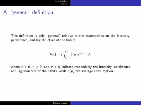
A “general” definition

This definition is only “general” relative to the assumptions on the intensity,persistence, and lag structure of the habits.

h(t) = ε

∫ t

t−τ

c(u)eη(u−t)du

where ε > 0, η ≥ 0, and τ > 0 indicate respectively the intensity, persistenceand lag structure of the habits, while c(u) the average consumption.

Mauro Bambi

IntroductionModel

Ryder and Heal (RES 1973): ε = η > 0 and τ → +∞.

Constantinides (JPE 1990): η > ε > 0, and τ → +∞.

Abel (AER 1990): discrete time and ε > 0, η = 0 and τ = 1.

However our definition does not include the specification of Ravn et al. (RES2006)

Microfoundation and Identification/Estimation.

Mauro Bambi

IntroductionModel

First Mechanism: It can be explained also (but not only) in a benchmark model,where τ → ∞.

Focus on the role of the habits’ intensity and persistence.

Second Mechanism: crucially depends on the lag structure of the habits. Thenwe need to study it in the general framework.

Mauro Bambi

IntroductionModel

Benchmark ModelGeneral Model

Benchmark Model

Representative agent:

maxc(t),k(t)

∫ ∞

0

(c(t)− h(t))1−γ

1− γe−ρtdt

s.t. k(t) = (A− δ)k(t)− c(t)

k(t) ≥ 0, c(t) ≥ h(t) ≥ 0

k(0) = k0, h(0) = h0

where

h(t) = ε

∫ t

−∞c(u)eη(u−t)du

Mauro Bambi

IntroductionModel


A market equilibrium is described by any trajectory {φ(t), k(t), h(t)}t≥0 whichsolves

k(t) = (A− δ)k(t)− φ(t)− h(t) (1)

h(t) = εφ(t) + (ε− η)h(t) (2)

φ(t) = φ0e1γ(A−δ−ρ)t (3)

subject to (i) the initial condition of capital, k(0) = k0, (ii) the initial conditionof habit, h(0) = h0, (iii) the transversality condition limt→∞ k(t)e−(A−δ)t = 0,and (iv) the inequality constraints, k(t) ≥ 0, and c(t) ≥ h(t) ≥ 0.

φ(t) = ψ(t)−1γ with ψ(t) the costate variable.

c(t) = φ(t) + h(t)

c(t) = c(t)

Mauro Bambi

IntroductionModel


In a standard AK model, without external habits, all the aggregate variables“jump” immediately to the balanced growth path where they grow at the rate

Γ =1

γ(A− δ − ρ)

then the economy faces positive growth if and only if:

A ≥ A = δ + ρ (4)

otherwise the economy shrinks over time.

Mauro Bambi

IntroductionModel


BGP and Transitional Dynamics

An economy with external addictive habits, and linear production, has:

i) a unique asymptotic and positive growth rate g = max(ε− η, Γ) and

ii) a unique general equilibrium path converging monotonically to the balancedgrowth path

if A ≥ A, k0 ≥ h01

A−δ−ε+ηand g < A− δ.

These results still hold when A < A and ε > η.

Mauro Bambi

IntroductionModel


What pins down a g = ε− η?

Intuitively these results depend on the inequality ε > η and on the habitaddiction which trigger a positive growth rate in the habit stock and in the

aggregate consumption.

Mauro Bambi

IntroductionModel


In fact, the representative consumer faces two constraints:

h(t) = (ε− η)h(t) + ε(c(t)− h(t)) and c(t) ≥ h(t)

At the equilibrium, the solution path of c(t), obtained by solving the represen-tative agent problem, coincides with the given path, c(t):

h(t) = (ε− η)h(t) + ε(c(t)− h(t)) ≥ (ε− η)h(t)

and then the habit stock, as well as aggregate consumption, grows at least atthe rate ε− η even if c(t)− h(t) shrinks over time at the rate Γ < 0.

Mauro Bambi

IntroductionModel


When is the growth rate sustainable?

Under two conditions:

I g < A− δ = r (standard requirement)

I h0 ≤ (A− δ − ε+ η)k0

Mauro Bambi

IntroductionModel


The last condition implies that h0 ≤ rk0 if ε = η;

Suppose does not hold, then c0 ≥ h0, only if an initial net disinvestment, i0 < 0,takes place. If this happens a positive growth rate of consumption and habits isclearly not sustainable over time because financed with a continuous selling ofassets which leads to zero capital stock in a finite time.

The condition becomes even more restrictive when ε > η.

Mauro Bambi

IntroductionModel


The First Mechanism:

Emerge when g = ε − η: transitional dynamics led by a “save now or regret itlater” mechanism:

the representative agent decides to consume, till the very beginning, less thanin the standard AK model in order to save enough and accumulate the capitalnecessary to keep over time the consumption level higher than the habits stockavoiding, in this way, an infinite disutility. The faster accumulation of capitalwill imply a higher consumption in the long run than the one in the AK modelwithout habits.

Habits reduce the desire to smooth consumption.

Mauro Bambi

IntroductionModel


0 100 200 300 400 5000

5

10

15

20

25

30

t

Capital Dynamics

0 100 200 300 400 5000.71

0.72

0.73

0.74

0.75

0.76

0.77

0.78

0.79

0.8

t

Saving Rate Dynamics

0 50 100 1500.15

0.2

0.25

0.3

0.35

0.4

0.45

0.5

t

Consumption Dynamics

AK with ε−η>Γ2>0

AK with no habit

AK with ε=η

Figure: Capital, saving rate and consumption dynamics when g = ε− η.

Mauro Bambi

IntroductionModel


General Model

Same model setup but now the habits are

h(t) = ε

∫ t

t−τ

c(u)eη(u−t)du

or differentiating it

h(t) = ε(c(t)− c(t − τ)e−ητ)− ηh(t)

In this framework the second mechanism can be studied. Before moving on it,

we come back quickly on the first mechanism.

Mauro Bambi

IntroductionModel


First mechanism with a finite lag structure:

The presence of a finite τ may reduce or even break down the mechanism fora positive growth rate in the habits and then the “save now or regret it later”mechanism.

The reason is that at the market equilibrium we have that

h(t) = ε(c(t)− c(t − τ)e−ητ)− ηh(t)

≥ (ε− η)h(t)− εc(t − τ)e−ητ

Mauro Bambi

IntroductionModel


On the second mechanism:

At the equilibrium c(t) = c(t) and c(t)−h(t) = φ0eΓt , then the habits formation

equation becomes:

h(t) = (ε− η)h(t) + εh(t − τ)e−ητ + g(t)

with g(t) = εφ0

(1− e−(Γ+η)τ

)eΓt .

Delay differential equation with forcing term. Endogenous fluctuations in thehabits and consumption.

Habits revised periodically and risk adverse agents.

Mauro Bambi

IntroductionModel


To analyze formally the first and second mechanism, we proceed as follows:

1. Describe the market equilibrium;

2. Find the asymptotic growth rate of consumption and habits;

3. Use it together with the transversality condition and the capital accumu-lation equation to completely describe the transitional dynamics of theeconomy by finding the general equilibrium path of the main aggregatevariables;

Mauro Bambi

IntroductionModel


Market Equilibrium

A market equilibrium is described by any trajectory {φ(t), k(t), h(t)}t≥0 whichsolves

k(t) = (A− δ)k(t)− φ0eΓt − h(t) (5)

h(t) = ε

∫ t

t−τ

[h(u) + φ0e

Γu]eη(u−t)du (6)

φ(t) = φ0eΓt (7)

subject to (i) the initial condition of capital, k(0) = k0, (ii) the past history ofhabit, h0(t), t ∈ [−τ, 0], and (iii) the transversality condition limt→∞ k(t)e−(A−δ)t =0 and (iv) satisfying k (t) ≥ 0 and c(t) ≥ h(t) ≥ 0.

Mauro Bambi

IntroductionModel


Asymptotic Growth Rate of Consumption and Habits

To find it the first step is to use a change of variable to rewrite the habits’equation (6) as an autonomous algebraic equation.

Then to study the spectrum of roots of its characteristic equation, which is:

∆(λ) = 0 with ∆(λ) = −1 + ε

∫ 0

−τ

e(Γ+λ+η)udu (8)

when Γ > 0.

Mauro Bambi

IntroductionModel


The spectrum of roots of (8) has a leading real root, α∗, which is positive if andonly if

ε− η > Γ and τ > τ∗ with τ∗ = −log

(ε−Γ−η

ε

)Γ + η

Moreover α∗ is an increasing function of τ and it converges to ε − Γ − η, asτ → ∞.

From now α∗ = α∗ + Γ.

We can now write the solution of the habits and consumption.

Mauro Bambi

IntroductionModel


The consumption dynamics is described by the equation

c(t) = σ0eα∗t + (1 + θ)φ0e

Γt︸︷︷︸trend component

+ χ2(t)eΓt︸︷︷︸

oscillatory component

(9)

with limt→∞ χ2 (t) e(Γ−α∗)t = 0 and σ0 = σ0(h0(t), φ0). Then the asymptotic

positive growth rate of consumption and the habit stock is

i) g = α∗ if ε− η > Γ and τ > τ∗, and σ0 = 0, or

ii) g = Γ if ε− η < Γ or ε− η > Γ and τ < τ∗, and φ0 = 0

where χ2(t) is the oscillatory component, coming from all the (infinite) roots

having real part lower than α∗.

Mauro Bambi

IntroductionModel


Balanced Growth and Transitional Dynamics

A market economy with a finite lag structure in the habits, and a high level oftechnology (Γ > 0) has

i) a unique asymptotic and positive growth rate g = max(Γ, α∗);

ii) a unique competitive equilibrium path which oscillatory converges over timeto the balanced growth path:

h(t) = σ0eα∗t + θφ0e

Γt + χ2(t)eΓt

c(t) = σ0eα∗t + (1 + θ)φ0e

Γt + χ2(t)eΓt

k(t) =σ0

A− δ − α∗ eα∗t +

φ0(1 + θ)

A− δ − ΓeΓt +

∫ ∞

t

χ2(u)e−(A−δ−Γ)(u−t)du

if A− δ > α∗, and (k0, h0(t)) such that φ0 = φ0(k0, h0(t)) ≥ 0.

Mauro Bambi

IntroductionModel


The explicit form of the last condition is

k(0) ≥ h(0)

A− δ + η − ε+ εe−(A−δ+η)τ− εe−(A−δ+η)τ

A− δ + η − ε+ εe−(A−δ+η)τ

∫ 0

−τ

e−(A−δ)uc (u) du

which converges to the condition in the benchmark model as τ → ∞.

It is also quite straightforward to observe that this condition is less restrictivethan in the benchmark model since

rk0 ≥ h0 = ε

∫ 0

−∞c(u)eηudu > ε

∫ 0

−τ

c(u)eηudu

Mauro Bambi

IntroductionModel


Moreover we have also found the conditions on the parameters which allow usto distinguish two types of the oscillatory behavior:

I Damping fluctuations around the balanced growth path;

I Small fluctuations smoothed out quickly; convergence is monotonic.

The taxonomy of the dynamics can be summarized in a figure under the normal-ization ∫ t

t−τ

eη(u−t)du = 1 t ≥ 0

Mauro Bambi

IntroductionModel


0 10

1

η

ε

Low Technology Case (Γ<0)

0 10

1

ηε

High Technology Case (Γ>0)

g=α* >0 and no dampingfluctuations around the

BGP

g=Γ >0 and no dampingfluctuations around the

BGP

g=Γ >0 and dampingfluctuations around the

BGP

α*>0 and no dampingfluctuations around

the BGP

α*<0 and no dampingfluctuations around

the BGP

−Γ

α*<0 and dampingfluctuations around

the BGP

α*>0 and dampingfluctuations around

the BGP

Figure: Taxonomy of the dynamics in the space (η, ε)

Mauro Bambi

IntroductionModel


Model calibration

Calibration of the benchmark model:

I along the balanced growth path where g = ε−η; ε and η can be calibratedto match the performance of the average U.S. annual output and utilitygrowth rates as observed in the data:

g = gu.s. = 0.02 and gu = 0

In fact, the main aggregate variables evolve along the balanced growthpath as follows:

h(t) = h0egt , c(t) = h(t), k(t) =

c(t)

r − g

Mauro Bambi

IntroductionModel


Alternatively:

I along the balanced growth path with g = Γ; any calibration of the pa-rameters usually used in the literature to induce a higher desire to smoothconsumption, violates the Easterlin’s hypothesis.

g = gu.s. but gu > 0

Is this violation quantitatively relevant?

The main aggregate variables evolve along the balanced growth path asfollows:

h(t) = h0egt , c(t) =

(Γ + η)h(t)

ε, k(t) =

c(t)

r − g

Mauro Bambi

IntroductionModel


This implies the following path of the instantaneous discounted utility

u(t) =[(g + η − ε)h0]

1−γ

ε1−γ(1− γ)e(g−r)t (10)

The two main parameters to be calibrated are γ and ρ.

We set ρ = 0.017 and γ = 1.1 or 2 or 2.8. (e.g. Campbell and Cochrane JEP1999).

Implied annual real interest rate is 3.9%, 5.7% and 7.3% respectively.

Discounted utility (10) always negative as well as the argument at the exponent.Wellbeing increases over time since the discounted disutility (−u) grows at

g−u = −0.019 g−u = −0.037 g−u = −0.053

Mauro Bambi

IntroductionModel


Among the three values of the interest rate, the latter implies the highestconsumption-output ratio:

r = 0.073 δ = 0.1 ⇒ c

y≃ 1

3

This value is still quite low when compared with the empirical evidences (aroundtwo-thirds).

This difference depends on how capital is defined in an AK model: capital shouldbe viewed broadly to include not only physical but also human capital.

However Jones et al. argue that investment in human capital are counted as pri-

vate consumption in national income accounts and for this reason a discrepancy

between the predicted and actual consumption-output ratio naturally emerge.

Mauro Bambi

IntroductionModel


0 15 30 45 60 75

−0.053

−0.037

−0.02

0

0.015

0.03

Quarters

Dis

coun

ted

inst

. dis

utili

ty g

row

th r

ate

on th

e B

GP

Easterlin’s hypothesis

α∗model prediction when g=

model prediction when g= Γ

Figure: Model predictions and the Easterlin’s hypothesis

Mauro Bambi

IntroductionModel


What happens when habits are characterized by a finite lag structure?

Calibration of the parameters ε and η in order to match the growth rate g =α∗ = 0.02.

To do so we need first to set a value for τ and then use the characteristic equationto find the values of ε and η, if any, which solve it and respect also the othertwo sign conditions introduced when we look at the consumption dynamics.

According to Crawford’s test on microeconomic panel data (see Crawford RES2010): τ = 2 quarters improves the agreement between theory and data withrespect to the one lag case without reducing too much the power of the test.

Then we set τ = 2 quarters and we find numerically that ε = 0.5543 and η = 0.1

are a good choice.

Mauro Bambi

IntroductionModel


More precisely τ = 2, ε = 0.5543 and η = 0.1 implies

−1 + ε

∫ 0

−τ

e(g+η)udu = 0

and τ∗ = − log( ε−Γ−ηε )

Γ+η= 1.9955 when g = 0.005, γ = 2, τ = 2, ε = 0.5543,

η = 0.1, r = 0.01, and ρ = 0.00425 at quarterly frequency.

This calibration matches both the average growth rate of the U.S. economy andthe Easterlin’s hypothesis;

Similar results emerge when we have tried for different value of r and τ .

Mauro Bambi

IntroductionModel


What about the second mechanism?

The positive value of Γ implies that the economy is always in the region of theparameter space where small deviations from the balanced growth path imply nodamping fluctuations around it.

On the other hand if we calibrate the model along the balanced growth path

where g = Γ the same conclusions as in the benchmark model hold but now de-

viations from the balanced growth path implies convergence toward it by damping

fluctuations.

Mauro Bambi

IntroductionModel


In fact for the values of ε in the range (0.093, 0.492) - Constantinides JEP 1990- we have found that damping fluctuations raise as long as

τ < 10.47 quarters when ε = 0.093

and

τ < 2.02 quarters when ε = 0.492

Mauro Bambi

IntroductionModel


Damping fluctuations Save now or Matchedaround the BGP regret it later moments

Benchmark model (τ = ∞)

g = ε − η no yes average output growthno utility growth

g = Γ no no average output growth

“General” model (τ = 1, 2 or 3)

g = α∗ no† yes average output growthno utility growth

g = Γ yes no average output growth

† The oscillatory component is smoothed out quickly and convergence to the BGP is monotonic.

Table: Summary of the Results

Mauro Bambi

IntroductionModel


Conclusion

I Taxonomy of the dynamics reveal a more complex relation betweenhabits and consumption than usually stressed by the literature.

I Calibration Exercise: first mechanism, holds independently by the lagstructure as soon as the targets to be matched are the average outputand utility growth rate. second mechanism not relevant under thiscalibration but it becomes relevant, when the model is calibrated asusually done in the literature, and habits lag structure is finite.

Mauro Bambi

Introduction Model - University of Yorkmb607/presentation_jmathe.pdf · Introduction Model Habit...

Documents

Transcript of Introduction Model - University of Yorkmb607/presentation_jmathe.pdf · Introduction Model Habit...