Sustainability considerations in the Design of Big Dams: Merowe, Nile Basin

Anthony ParisTeresa YamanaSuzanne Young

Prof. El Fatih Eltahir, Advisor

1.096

1

May 19, 2004

Introduction

Any large engineering project requires a team with expertise in multiple branches of engineering. A dam project will include mechanical, electrical and civil engineers just for the design of the dam itself. Each of these engineers will have their own concerns and priorities that they try to incorporate into the design process. The team would meet to discuss these different requirements and attempt to come up with an optimal design. The role of an environmental engineer in this situation would be to analyze the effects of the environment on the project, and the effect of the project on the environment. The environmental analysis will shed light on crucial large-scale and long-term effects that might not have been foreseen. Ideally this would be an iterative process; the environmental engineer would conduct an analysis based on the design being proposed, and make certain recommendations that would then be incorporated into the next version of the design.

Our goal for this project is to take on the role of the environmental engineers in the Merowe Dam project. Based on the design specifications proposed for the Merowe Dam, we will conduct an environmental analysis and make recommendations to improve the dam’s productivity and lessen its negative impacts. We have chosen three areas of focus. First, we will analyze how changes in river flow caused by climate change will affect the Merowe Dam’s power

2

capacity. Second, we will analyze deposition of sediments in the dam reservoir, and based on these calculations, estimate the useful lifetime of the dam. Third, we will discuss the effect of the Merowe Dam on public health, particularly in terms of the transmission of malaria and schistosomiasis. For each of these three areas, we will make recommendations on how we might change the operating parameters or dimensions of the dam in order to extend its productivity and lessen its negative impacts.

Merowe Dam Project Overview

Sudan, Africa’s largest country by landmass and one of its poorest, is a developing country that needs energy for economic growth and development. A 19-year old civil war has caused Sudan’s economy to stall. The current combined electricity generation is up to 500 megawatts (MW), while daily demand is estimated at about 1000 MW. Power blackouts are common in Sudan, “crippling businesses that cannot afford their own generators and pushing up operational costs for those that can” (BBC 2002).

To eliminate the current electricity deficit and satisfy future demand, the Sudanese government will utilize the waters of the Nile River to generate electric power by installing the Merowe Dam. Hydropower is recognized as a renewable and clean energy source, and its link to water management is considered to play a unique role in sustainable development (Ogunbiyi and Norris 2003). Though the

3

potential for hydroelectric power plants along Africa’s water systems is huge, estimates say that only between 3-16% of the continent’s hydro potential has been exploited so far (World Economic Forum 2003). The Merowe (pronounced “Mirowy”) Dam, previously known as the Hamdab Dam, is named after a small island 400 km (250 miles) north of the capital Khartoum through which the structure of the dam will cut (NCAM). Costing $1.73 billion, it will have ten turbines with a total capacity of 1,250 MW when completed, three times Sudan’s current capacity (Sudan Tribune 2003). This dam will also contribute to Sudan’s industrial and agricultural development, as well as the employment and improvement of the standard of living of the citizens of Sudan (Arab Fund 2003). Furthermore, the dam will be able to hold back water such that areas downstream will no longer experience floods (BBC 2002).

The Anglo-Egyptian administration in Sudan first proposed the idea of building a dam at the fourth cataract of the Nile River in 1943 (NCAM). Several decades later, in 1979, Sudan’s Ministry of Irrigation concluded that pending further feasibility studies, the river reach above Merowe at the fourth cataract on the Main Nile is the right location for the country’s next hydroelectric project. However, it was not until the present government came to power in 1989 that the building of the dam became a top priority to provide more electricity and reduce flooding (NCAM). This dam also has a political motivation. The government hopes that it will bring hope to a nation torn by civil war and instability in the surrounding region.

The general shape of the Main Nile valley at the fourth cataract consists of a wide river bed with fairly low banks sloping gently up above the river level. The design of the dam is therefore long in relation to its height with extended and elaborate spillway structures. The dam consists essentially of a concrete structure in the main river channel and a rockfill dyke on each bank, and will impound a

4

reservoir with an active storage capacity of 8.3 billion cubic meters (Ministry of Irrigation 1979). Table 1 shows the principal characteristics of dam features. Figure 1 shows the general arrangement of the dam.

Figure 1 – General arrangement of Merowe Dam

Table 1. Principal characteristics of dam features.

5

DAM    Height (above river bed) m 60Length (along crest) m 9320 Concrete faced rockfill dam (right bank) m 4800 Rock and earthfill dam (left bank) m 4000 Concrete dam* (main river channel) m 520RESERVOIR  Length km 160Surface area km2 476Active storage volume Minimum storage level Maximum storage level

106m3

mm

8300290296

POWER FACILITY    Installed turbine capacity MW 1250No of units 10Capacity of each unit MW 125

*Includes powerhouse for 10 turbines units and other major equipment, spillway, other appurtenant structures, associated intakes, outlets, and control valves.

According to Sudan’s Ministry of Irrigation, “the surface

spillways are used in conjunction with deep sluices to control flood flows. During the dry season these deep sluices would also permit a drawdown of the reservoir if necessary in case of emergency. Furthermore, they might be used every year to effect a partial drawdown just prior to the flood, and to operate the reservoir at a relatively low level during the period of highest sediment concentration (mainly August and the beginning of September). Such a drawdown will reduce the power output, but on the other hand it

6

will also minimize the sedimentation effects further upstream from the reservoir area” (1979).

After bidding by several international firms for construction of the dam, the contract for Merowe Dam Project Civil Engineering Works was awarded to the joint venture of China International Water & Electric Corporation and China National Water Resources and Hydropower Engineering Corporation. Construction began in December 2003. France’s Alstom Group won the contract to supply the turbines and generators for the dam. The first turbine will come online in 2007, while all ten turbines are expected to be fully operational by July 31, 2008. Funding for the Project will be provided by the government of Sudan supported by loans from the following funding agencies: Arab Fund for Economic and Social Development, The Saudi Fund for Development, Kuwait Fund for Arab Economic Development and Abu Dhabi Fund for Development.

7

Nile Hydrology

General Facts

The Nile River is 6700 km. It traverses international boundaries and travels through 13 riparian countries. It has a total Catchment Area of 3 million km2 It’s average runoff is 30 mm. The major contributors of the total flow come from the East African lake region and the Ethiopian Highlands. The Nile has three main tributaries, including the White Nile, Blue Nile and the Main Nile. This river crosses an extremely wide band of latitude originating about 4oS and emptying at 32oN.

Flow Patterns

There are three main tributaries that feed into the Main Nile, and these are the White Nile, the Blue Nile, and the river Atbara. The Nile River’s hydrology is highly influenced by the monsoon season. During the months of July-November the river Atbara and the Blue Nile contributes approximately 5/7 of the Nile’s mean annual flow. Contrarily, the White Nile is not perennial, and as such, it produces a steady baseflow year around.

8

Figure 2 – Annual flow pattern of Nile

In order to better grasp the over all picture of the Nile flow patters we can do the following exercise. Taking an average annual flow of 84 km3 and dividing this into 7 units of 12 km3 each, we can then assign these units to tributaries. (Eltahir, 1996) Thus, four units will come from the Blue Nile, two units from the White Nile, and one unit from the river Atbara.

Dams

There are a number of dams that exist along the Nile already which include: Aswan, Khashm el Girba, Jebel Aulia Dam, Sennar Dam, Roseires Dam, and Owen Falls Dam. These dams disrupt the natural flow of the river, and traps sediments that would have normally gone to the Mediterranean Nile delta.

9

The Components Parts

The component parts that make up the Nile River’s watershed are:

1) The Lake Victoria Basin 2) The East African Lakes below Lake Victoria 3) The Bahr el Jebel and the Sudd 4) The Bahr el Ghaal Basin 5) The Sobat Basin and the Machar Marshes 6) The White Nile below Malakal 7) The Blue Nile and its Tributaries 8) The Atbara and Main Nile to Wadi Halfa 9) and the Main Nile in Egypt.

The Lake Victoria Basin has an annual rainfall of 1151 mm contributing to approximately 122 km3/yr to the flow. Its tributaries contribute approximately 276 mm or 22.4 km3/yr while evaporation accounts for 1116 mm or 107 km3/yr. The resulting outflow from this system is 311 mm or 39.8 km3/yr. This provides a relatively steady baseflow for the river.

The East African Lakes below Lake Victoria includes lake Albert, lake Kyoga, and lake Edward. Rainfall contributes to about 10.3 km3/yr its tributaries contribute about 10.6 km3/yr and 16.3 km3/yr is evaporated. Thus, the resulting outflow is approximately 45 km3/yr. The outflow contribution to Nile is dominated by lake Victoria. This region has also had a dramatic variation in flow level historically.

The Bahr el Jebel and the Sudd receives an annual rainfall of 871 mm while evaporation in the area is much higher at 2150 mm. This area of Nile reaches is the most complex to having many seasonal inflows. It is littered with permanent swamp land and has seasonal flood plains that are inundated. The high levels of evaporation and

10

transpiration come from the wide distribution of the river area of the water and from the large amounts of vegetation (i.e. papyrus). There is little seasonal variation with annual outflow which equals to about half of the inflow. The Jonglei Canal was created in order to provide a more direct way of the water traveling through this region in order to stem the evaporation losses incurred in this area.

The Bahr el Ghaal Basin outflow to the White Nile is almost negligible which amounts to less than 3%. The upper basins have relatively high rainfall, but the river flow spills over into the many flood plain areas resulting in almost total lost to evaporation. The sediment loads of these rivers if greater than lake-fed Bahr el Jebel and they have a higher potential for alluvial channels.

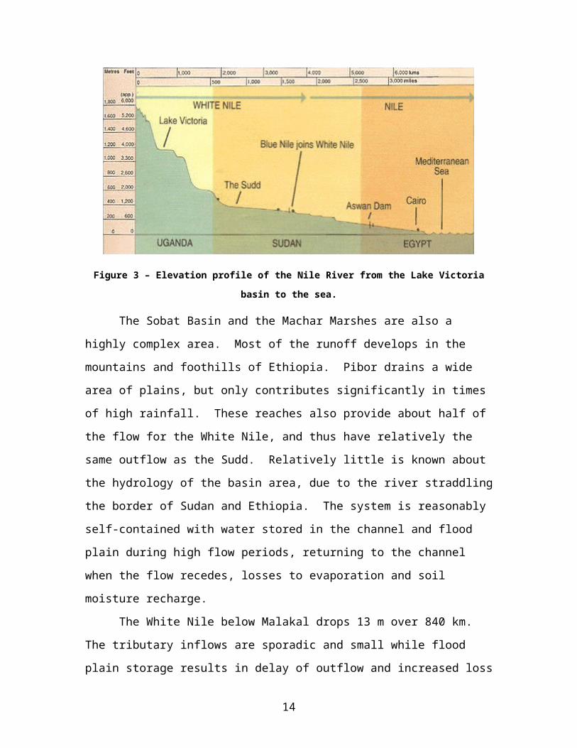
Figure 3 – Elevation profile of the Nile River from the Lake Victoria basin to the sea.

The Sobat Basin and the Machar Marshes are also a highly complex area. Most of the runoff develops in the mountains and foothills of Ethiopia. Pibor drains a wide area of plains, but only contributes significantly in times of high rainfall. These reaches also provide about half of the flow for the White Nile, and thus have relatively the same outflow as the Sudd. Relatively little is known about the hydrology of the basin area, due to the river straddling the

11

border of Sudan and Ethiopia. The system is reasonably self-contained with water stored in the channel and flood plain during high flow periods, returning to the channel when the flow recedes, losses to evaporation and soil moisture recharge.

The White Nile below Malakal drops 13 m over 840 km. The tributary inflows are sporadic and small while flood plain storage results in delay of outflow and increased loss to evaporation. The Jebel Aulia dam further raised upstream river levels after June 1937. Irrigation and evaporation have led to increased losses. Outflow is delayed to supplement the Blue Nile in low flow season due to the dam as well. The Sudd provides the baseflow component while the Sobat basin contributes the seasonal component.

The Blue Nile and its Tributaries provides the greater part of flow of the Main Nile approximated at 60%. Limited information is known about this area’s hydrology, especially in its upper basin within Ethiopia. Its reaches begins in the Ethiopian Plateauat elevations averaging 2000-3000 m, peaking at 4000 m. The terrain consists of very broken and hilly, grassy uplands, swamp valleys, and scattered trees. It travels through deep ravines and canyons which drop to a depth of ~1300m at places. Near the headwaters of the Blue Nile and its tributaries lies Lake Tana at 1800 m above sea level. The lakes surface area is 3000 km2. The Blue Nile leaves and travels through series of cataracts through the Sudanese’s Plains sloping westward from about 700 m. The region it pasts through in the plains are covered with Savannah or thorn scrub. Its major tributaries are the Rahad and the Dinder. It has some wetland areas like Dabus that is around 900 km2 in area, and smaller swamps like Didessa. Upon its length are the Roseires Dam (2.4 km2) and Sennar Dam (0.5 km2). It is the single largest contributor to sediments in the Main Nile, averaging at 140- million tones per year.

12

The Atbara and Main Nile to Wadi Halfa is the convergence of White Nile and the Blue Nile at Khartoum. The river Atbara is the only major tributary that exists after Khartoum. The river Atbara drains northern Ethiopia (68,800 km2) and the mountains north of Lake Tana (31,400 km2). Most of its terrain type consists of arid plains dotted with low hills and rock outcrops

The Main Nile in Egypt is the last major stretch of the Nile before entering the Mediterranean. There are no flows generated below the Atbara confluence. The major infrastructure project of Aswan High Dam has dramatically changed the hydrology of the Main Nile. This project now stores most of the flood waters that produced during the monsoon season. Thus, the flood plains on the Nile are no longer inundated. Approximately1/3 of the river water is lost to reservoir evaporation. The project allows increased water availability for irrigation, hydroelectric, and a steady downstream flow. (Sutcliffe et. al., 1999)

13

The Model

The relationship between water elevation, storage volume, and surface area of the reservoir were analyzed in ArcGis 3.1. The analysis was based on topographical data from the Hydro1k project. Hydro1k is a suite of topographical data compiled by the U.S. Geographical Survey in order to help standardize research. The digital elevation model (DEM) for Africa was downloaded from the Hydro1k website, located at http://edcdaac.usgs.gov/gtopo30/hydro/. A shapefile polygon was created in the approximate region of the reservoir, starting along the edge of the dam and then upstream for a distance comparable to the length of reservoir estimated in the planning documents. The polygon was converted to a coverage file, and the DEM was converted to a grid. The DEM grid was clipped to the shape of the polygon using ArcInfo.

14

Figure 4 – DEM Polygon for Reservoir Area

The result was a polygon bounded on one edge by the proposed dam. The Spatial Analyst in ArcGis was used to determine 2D and 3D surface areas and the volume of the reservoir at various elevations by calculating the area and volume below the horizontal plane the given elevation. The areas and volumes were entered into Microsoft Excel and plotted against height. Lines were fit to the plots in order to develop equations describing Area-Height and Volume-Height relationships. The heights are expressed in the charts as meters above the river bed, which is located at 263 m above sea level.

15

y = 0.1843x2 + 11.561x + 71.655R2 = 0.9995

0

100

200

300

400

500

600

700

800

0 5 10 15 20 25 30 35 40

elevation above river bed (m)

2D- s

urfa

ce a

rea

(km

^2)

Figure 5 – Surface Area to Height Relationship

y = 0.0098x2 - 0.0311x + 0.394R2 = 0.9997

0

2

4

6

8

10

12

14

0 5 10 15 20 25 30 35 40

elevation above river bed (m)

stor

age

(km

^3)

Figure 6 – Volume to Height Relationship

It should be noted that these reservoir characteristics are based solely on the topography of the region. A more accurate analysis would take into account the effect the dam would have on the river

16

further upstream. The Nile River would experience gradually varied flow, and slope upwards as it approaches the reservoir.

In order to simulate the reservoir and the dam, we developed a simple model using Matlab. The model reads in Nile flow data from files. For our basic analysis, we used the average monthly flow interpolated to daily numbers, and repeated this for two years. We also conducted an analysis using actual monthly flow data measured in the Nile River between 1872 and 1986. The evaporation data was interpolated to daily values from daily averages. (Shahin, 1985)

The model loops through daily flow data for the desired number of years. It determines the new reservoir volume by adding daily inflow subtracting daily outflow, which in this case is only evaporation, to the previous day’s volume:

V= V_lookback + nile_inflow – evaporation

The volume of water below the turbine intakes was subtracted from the total volume in order to find the active volume; this is the amount of water that can pass through the turbines, or be released through the sluices and spillways.

It then determines what portion of this volume should be available to flow through the turbines, according to the operation parameters that we specify. The first variation, also known as the pessimistic model, generates as much power as possible any given day, and does not consider the need for storage. We call it the pessimistic model because it acts as though the world might end tomorrow. The second variation, or the gradual release model, does take storage into account. It checks to see whether the inflow on any given day is greater than the yearly average inflow. If it is, it uses as much water as possible. However, if there is less than average inflow, the model assumes that it is the dry season, and begins to ration the

17

stored water. The volume of stored water on the first day of the dry season is divided by the average number of days in a year with less than average flow, which we found to be 240. This quantity is the amount of stored water that can be used each day. The volume released each day becomes the inflow for that day minus evaporation, plus the rationed amount of stored water. The third variation, called the constant head model, is very simple. The volume it sends through the turbines each day is equal to the inflow minus evaporation; it never uses stored volume, and the head, area and volume remain constant throughout the year. Whatever volume the model decides to use is called the usable volume.

We assumed that the maximum number of turbines that should be operating at any time is eight, so that there are still two on reserve to prevent unexpected blackouts should one of the turbines fail. If the usable volume is greater than or equal to the maximum volume that can enter the turbines, in this case 8 turbines x 200 cms/turbine x 86400 seconds, or 1.38 x 108 m3, the model switches on all 8 turbines. Otherwise, it determines how many turbines to use by dividing the usable volume by the turbine capacity and rounding down to the nearest whole number.

The water level of the reservoir was determined using the volume-height analysis. The amount of power generated is calculated using the following equation:

P=E * gamma * Q_turbine*head

Where P is power in Watts, E is the efficiency of the turbines, assumed to be 0.8, and head is the difference between water level of the reservoir and the power outlet. Q_turbine is the flow rate through the turbines, which is equal to the 200 cms times the number of turbines operating.

18

The volume passing through the turbines is subtracted from the reservoir volume, and the new height is calculated. If this new height is still greater than the maximum height, all excess water is discharged, either through the spillway or the controlled sluices. The area is calculated using the height-area relationship. Average yearly power calculated and variables are plotted. Figure 7 shows the output of the three variations being run with monthly average inflows. From top to bottom, the plots show Nile inflow in cms, evaporation in m3, reservoir volume in m3, water height in m, surface area of reservoir in m2, number of turbines in use, and power generated in watts. The graphs of height for Variations 1 and 2 show peaks on either side of the plateau in the dry season. We believe that this is a programming glitch resulting from calling the height-to-volume and volume-to-height functions consecutively. The height-to-volume relationship was found by fitting an equation to the topography data using Excel. This equation was inverted to find the volume-to-height relationship, but is not entirely accurate. A possible explanation for this is that the equation given by Excel did not have enough significant figures to be properly inverted. The peaks in the area graphs occur because area is directly related to height. Although the peaks are more pronounced in the Variation 2 graph, they are similar in size to the Variation 1 graph; the scales are different.

19

Figure 7 –Output for average inflow of the 3 different model variations

Of these three models, Variation 1 generates the most power per year, followed closely by Variation 2. The differences between the three models, as well as some of their advantages and disadvantages are discussed in greater detail later in this paper.

**Commented Matlab code for our function and corresponding functions is provided in Appendix A.

Climate

Climate change, Nile flows and hydropower

20

In order to assess how climate change will impact the engineering design of the Merowe dam, it is important to first understand the greenhouse effect and its connection to global warming and the height of Nile floods. It is then necessary to predict Nile floods for future years in order to have an understanding of the amount of electricity we expect the dam to produce. This is done by looking at historical Nile flows and using general circulation models to assess effects of climate change. In addition to climate, both operating parameters and design parameters play a role in determining the amount of hydropower generated.

Greehouse effect and global warming

As early as the 19th century, a Swedish scientist postulated that the combustion of fossil fuels may be an anthropogenic cause of climate change. The role of carbon dioxide, water vapor, and other “greenhouse” gases in the atmosphere’s heat retention capacity has come into sharper focus in recent decades (AIP 2004b). The theory that gases in the atmosphere cause a "greenhouse effect" that affects the planet's temperature was all but confirmed in 1958 by a French-Soviet drilling team at Vostok Station in central Antarctica. In a two kilometer long ice core they found a 150,000-year record that contained a complete ice age cycle of warmth, cold and warmth. It showed that the level of atmospheric CO2 had gone up and down in remarkably close step with temperature (AIP 2004a). In an earlier experiment at Mauna Loa Observatory, a man named Keeling found that atmospheric concentrations of CO2 were increasing linearly at 1 ppm/year. This led many to believe that the planet was undergoing “global warming.”

Scientists have also documented other changes in the chemical composition of the atmosphere, including increases in methane (CH4)

21

and nitrous oxide (N2O) since 1750 (IPCC 2001b). The U.S. and European governments have carried out many studies on global warming and climate change. Although most studies agree that global temperatures will rise, in terms of regional effects, uncertainties abound.

Historical Nile flows

So what does this have to do with Nile flows? Historical records of Nile floods reveal a strong correlation between low Nile floods and cold summers in Europe, and conversely, high Nile floods and warms summers in Europe (Hassan 1998). Fluctuations in Nile flood levels coincide with climatic changes in the Sahel and even the flow of the Senegal River at the other end of Africa (Hassan 1998). Warmer temperatures increase evapotransporation which in turn cause higher precipitation, leading to higher Nile floods. Climate change clearly influences the height of Nile floods.

The long term annual average of Nile flows at Aswan between 1872-1986 is 88 km3, with a standard deviation of 14 km3. The floods typically occur between the months July-September. Figure 9 shows graphical representations of the average monthly Nile flows and Figure 8 shows a record of annual Nile flows, both 1872-1986. There is substantial interannual variability in the Nile flows, with a maximum annual yield of 128 km3 in 1879 compared to a minimum of 46 km3 in 1913. There is also substantial interdecadal variability. The mean annual discharge between 1943-1969 is 88 km3, which is equal to the long term annual average between 1872-1986. The mean annual discharge between 1872-1898 is 102 km3, a 15% increase from the long term average, whereas the mean annual discharge between 1979-1986 is 74 km3, a 15% decrease.

22

Nile discharge, 1872-1986

40

50

60

70

80

90

100

110

120

130

1870 1880 1890 1900 1910 1920 1930 1940 1950 1960 1970 1980

Ann

ual d

isch

arge

(km

^3/y

ear)

Longterm annual average = 88.1 km^3/year

Figure 8 -- Annual Nile discharge, 1872-1986

Average Longterm Monthly Nile flows, 1872-1986

0

5

10

15

20

25

January February March April May June July August September October November December

Dis

char

ge (k

m^3

/mon

th)

Figure 9 -- Average monthly Nile flows, 1872-1986

Climate in the Sudan region

23

The seasonal relative movement of the sun and the associated inter-tropical convergence zone (ITCZ) mainly influence Sudan’s climate. Merowe has an arid, or hot and dry, climate. Average summers are very hot (34°C) and winters relatively cold (20°C), though temperatures can reach a maximum of 43.3C and a minimum of 4.4C (Lahmeyer 2001). Northern Sudan’s rainy season occurs between July and August. There is almost no rainfall—the mean annual rainfall in Merowe is only 50 mm, but this is quite variable, as the deviation from the average annual rainfall that may be expected in half the years in the north is about 100%. Showers and storms are generally similar throughout the Sudan. According to Sudan’s Ministry of Irrigation, “the variation of total rainfall is due almost entirely to the variation in the number of storms occurring rather than any variation of the intensity of storm rainfall. The average rainfall on a rainy day is about 13 mm throughout Sudan. Thus, even in areas with low annual rainfall, the rain falls in short intense showers which can cause extensive flooding” (1979).

However, global warming may increase the intensities of storms. A 1991 IPCC study showed that 1-3°C in global temperatures by the year 2030 is expected to cause more intensive weather activity, resulting in more severe and frequent flood droughts (Ribot 1996). This may also decrease hydropower potential in drought prone regions (IPCC 2001b).

General Mean Circulation models

General circulation models (GCMs) are mathematical representations (i.e. computer simulations) of atmospheric and oceanic properties and processes that attempt to describe earth's climate system. Developed in 1960s, they have become the chief tools in analyzing effects of climate change (AIP 2004b). In the 1980s, a

24

global body of climate scientists, the Intergovernmental Panel on Climate Change (IPCC), was formed to provide scientific advice to growing international political negotiations over how to respond to climatic change.

There are several different GCM scenarios in use, including: UKMO (United Kingdom Meteorological Office), GISS (Goddard Institute for Space Studies, New York, NY), GFDL (Geophysical Fluid Dynamics Laboratory steady-state, Princeton, NJ), GFDLT (Geophysical Fluid Dynamics Laboratory transient, Princeton, NJ), MPI (Max Plank Institute, Hamburg, Germany), and CCC (Canadian Center for Climate, Victoria, Canada).

Literature review of predicted flows

Appendix B summarizes a literature review on climate change in the Nile basin region and predicted changes in Nile flows. While nearly all studies agreed that temperatures will increase, precipitation predictions are less certain. Predictions of response by the Nile to increasing temperatures vary widely; different simulations give conflicting results. The summary of Yates (1998b) results shown in Figure 10 an example of how widely results vary. The two numbers on ends of each line represent extreme discharges of six different GCM scenarios, whereas the boxed number is the historic long term average. Additional tick marks on each line are remaining GCM scenarios, which indicate range of climate change induced flows at different points in the Nile Basin. Five of the six GCMs showed increased flows at Aswan, with increases as much as 137%. (UKMO). Only one GCM showed a decline in annual discharge at Aswan (-15%). All numbers are in the units of cubic kilometers per year.

25

Figure 10 – Range of discharges for major points along the Nile. (Yates, 1998)

The IPCC notes that because the Nile and other major rivers in Africa “originate within the tropics, where temperatures are high, evaporative losses also are high in comparison to rivers in temperate regions. Elevated temperatures will enhance evaporative losses; unless they are compensated by increased precipitation, runoff is likely to be further reduced” (IPCC, 2001a).

Predictions in Strzepek (1995) vary from 78% flow reduction in the GFDL simulation to a 30% increase in the GISS model. These results are confounded by Yates (1998a) predictions, which vary from 9% flow reduction (GFDL) to a 64% increase in the GISS model. Model results indicated that the Nile basin is quite sensitive to changes in precipitation. Hulme (1994) concludes Nile discharge will decline due to greater evaporation; specifically, it predicts reduced Blue Nile flows and constant or slightly increased White Nile flows. Similarly, Sene’s (2001) model results suggest a slight increase in White Nile flows.

In short, the literature review confirms that there is a lot of uncertainty in predicting future Nile flows. To take into account this

26

uncertainty, it is important to test the performance of the Merowe Dam under different scenarios of climate change.

Scenarios in model

The following three climate scenarios are used to test the performance of the Merowe Dam: no change (assume Nile flows remain at the 88 km3/year long term average); wetter climate (Nile flows increase by 15% or one standard deviation to 102 km3/year); drier climate (Nile flows decrease by 15% or one standard deviation to 74 km3/year). As previously mentioned, Nile flows between 1872-1986 show high interdecadal variability, with groups of years corresponding to each of the three scenarios above (see Table 2).

Table 2. Definition of climate scenarios runs in model, based on flow data in Figure 8.

Climate scenario YearsAverage

flowDeviation from

long term

    [km3/yr]average 88

km3/yr

No change1943-1969 88 --

Wetter climate1872-1898 102 +15%

Drier climate1979-1986 74 -15%

27

These three climate scenarios were run both in the version of the MATLAB model that reduces the variability in the hydropower generated by rationing the stored water and gradually releasing it during the dry season (variation 2, or var 2) and the pessimistic version of the model that uses up the stored water as quickly as possible (variation 1, or var 1). While the latter produces slightly more hydropower than the former, it may be more realistic to ration the stored water and decrease the number of turbines gradually rather than have a sudden drop off at the end of the wet season. In addition, the maximum storage height of the reservoir (in other words, the height of the spillway) was varied between 294-298 m. This design parameter in effect translates to the size of the reservoir. The baseline case is run at 296 m. The results of the model will reflect how the uncertainty of climate change induced Nile flows and the size of the reservoir affect power generation of the Merowe Dam.

Equation (1) shows the equation that the MATLAB model uses to calculate hydropower, where “gamma” (γ) is defined by Equation (2):

Power = eγQh(1)

γ = ρg(2)

The variables are defined as follows: e is the efficiency coefficient of the turbines, assumed to be 0.8; ρ is the density of water, which is 1000 kg/m3; g is gravity, which is 9.8 m/s2; Q is the flow of water into the intake of the powerhouse, in units [m3/s]; and h is the drop in head

28

between the intake to the powerhouse and the outlet to the river, in units [m].

Results

Table 3. The annual average power [watts] generated for each climate scenario at each maximum storage reservoir height, run in the

pessimistic model (var 1).

Maximum storage height of reservoir [m]Climate scenario 294 295 296 297 298

No change 2.09E+11 2.14E+11 2.20E+11 2.25E+11 2.30E+11

Wetter climate 2.13E+11 2.19E+11 2.25E+11 2.30E+11 2.35E+11

Drier climate 2.11E+11 2.16E+11 2.21E+11 2.27E+11 2.32E+11

Table 4. The annual average power [watts] generated for each climate scenario at each maximum storage reservoir height, run in the ration

stored water model (var 2).

Maximum storage height of reservoir [m]Climate scenario 294 295 296 297 298

No change 2.03E+11 2.08E+11 2.13E+11 2.18E+11 2.23E+11

Wetter climate 2.07E+11 2.12E+11 2.17E+11 2.22E+11 2.26E+11

Drier climate 2.06E+11 2.12E+11 2.17E+11 2.22E+11 2.27E+11

As expected, a wetter climate generates the most hydropower of the three climate scenarios, and the higher the maximum storage height of the reservoir, the more electricity produced (linear relationship). Each one meter increase in maximum storage height of the reservoir yields about a 10% increase in hydropower generated.

29

Figures 11-13 show that the model that rations the stored water over the dry season (var 2) produces less electricity than the model that uses up the stored water as quickly as possible (var 1) in all three climate scenarios.

Figure 11 – No Change in Climate

30

Figure 12 – Wetter Climate

Figure 13 – Drier Climate

31

Recall that the definition of wetter climate is defined in this study as a 15% increase in flow, and that a drier climate is a 15% decrease in flow. The results show that the hydropower generated in the wetter climate for the pessimistic model (var 1) is roughly 30% higher (or two standard deviations greater) than the hydropower generated in the climate with no change.

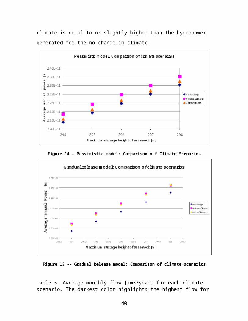
Surprisingly, both variations of the model show that the drier climate produces more electricity than the climate with no change (and in variation 2 of the model, the drier climate hydropower is also equal to or greater than the wetter climate hydropower). This could be due to the intermonthly flows during the ranges of years chosen to represent each climate scenario, i.e. wetter climate (1872-1898), no change in climate (1943-1969), drier climate (1979-1986). Table X shows the average monthly flow [km3/year] for each climate scenario. Though the average annual flow for wetter years is the highest (102 km3/year), the average monthly flows for wetter years are not always the highest, namely between April-July. Note that the average monthly flows for drier years are the highest for the months April-June, even though the average annual flow is only 74 km3/year. This could explain why in both models (var 1 and var 2) the hydropower generated for the drier climate is equal to or slightly higher than the hydropower generated for the no change in climate.

32

Figure 14 – Pessimistic model: Comparison o f Climate Scenarios

Figure 15 -- Gradual Release model: Comparison of climate scenarios

Table 5. Average monthly flow [km3/year] for each climate scenario. The darkest color highlights the highest flow for any given month, while the lightest color highlights the lowest flow.

Climate ScenarioWetterNo change Drier

January 4.95 3.82 3.30

33

February 3.44 2.84 2.60March 2.79 2.21 2.17April 2.01 1.91 3.20May 1.71 1.95 2.81June 2.04 2.55 2.74July 6.02 6.92 4.87August 20.84 18.5014.79September 25.05 20.7718.24October 17.30 14.12 9.95November 9.53 7.62 5.36December 6.70 4.88 3.97Annual 102.39 88.0973.54

Recommendation

Purely from a hydropower generation perspective, it is ideal to use variation 1 of the MATLAB model as a basis for dam operating parameters. Though stored water is used up as quickly as possible, the maximum number of turbines operates for as long as possible, generating more electricity than either of the other model variations. Though a higher maximum storage level for the reservoir does produce more electricity, it is unclear whether this recommendation is cost-effective.

34

Sedimentation

Introduction

Dams on the Nile River create artificial reservoirs that divert sediments. The dams’ reservoirs are filling with sediment instead of supplying the flood plains and the Nile delta in the Mediterranean with alluvium. Some negative reallocation of these sediment causes 1) coastal erosion, and 2) disrupts the marine food web indicated by the decline of sardine populations.

35

Process of Sedimentation Sedimentation is a highly complex process that involves:

1. Erosion2. Transportation3. Deposition4. Compaction

The detachment of particles in the erosion process occurs through weathering. Rocks are chemically altered or dissolved, or it is broken down by the kinetic energy of falling rain drops or running streams. The resulting rock fragments must be entrained before it can be transported away. Both entrainment and transport depends heavily upon the weight, shape, size, and the forces exerted on the particle by the flow. Deposition occurs when the forces diminish enough to result in a reduction or cessation of transport.

Erosion: Sources of Nile Sediment

Most of the sedimentation of the Nile originates from the Ethiopian highlands and flows through the Blue Nile and the Atbara. The White Nile and its tributaries lose most of its sediment load by spilling and deposition over flood plains, lakes, and marshlands. Thus, nearly all of the sediment (~90%) comes from the Blue Nile during the flood season (July-October). The total annual sediment load varies between 50 and 228 million tones. (Abu El-Ata, 1978)

Transportation

36

The While Nile provides the base flow of a mean average ~80 m3/day but deposits its sediment in wetlands before it flows into the Nile (Sutcliffe et. al). The main sediment load of the Main Nile comes from the Blue Nile and the Atbara. These rivers are perennial which flow primarily during the monsoon season (July to October). Thus, the monsoon season is critical for the mobilizing of sediments that originate in the Ethiopian Highlands. Sediment is carried and transported in two forms :

Suspension, where particulates are suspended in the water column

Bed-load, where sediment is moved along the river bed.

The Blue Nile transports both pebbles and boulders from its headwaters down towards the Main Nile, and is deposited in the Roseires reservoir on the way. As the slope of the Blue Nile diminishes, so does the mean size of the transported sediment. This is extremely characteristic of alluvial rivers.

There are two possible causes for this:

friction between the particles as they are transported along the river channel reduces their size

steeper slopes indicate higher flow velocities that enable transport of larger particles but as slope decreases so does flow velocity and the transport capacity of the fluid.

Ultimately the coarser grained sediment is mostly left behind resulting in a mixture of little gravel-sized material and finer grain sediment reaching the main river.

37

Currently there is no reliable means of measuring bed-load in the Nile. Hurst that was based on bed-load in similar rivers made an estimate of 25% bed-load. (Hurst, 1978) However, there is no evidence of an increasing rise of the river bed upstream of the Aswan Low Dam.

By the time that the Blue Nile and the Atbara reach the Main Nile, we see an almost total loss of coarse sediment. The resulting distribution of the total suspended sediment is: Clay (< 0.002 mm) 30%, Silt (0.002-0.02 mm) 40%, Fine Sand (0.02-0.2 mm) 30%. (Sutcliffe et. al.)

Deposition: Reservoir

Deposition is the counterpart of erosion. The final depositional area for the Nile sediments is the Mediterranean Sea delta. When river flow enters a reservoir, its velocity and transport capacity is reduced and its sediment load is eventually deposited. The amount and rate of deposition is determined mainly by detention storage time, the shape of the reservoir, and if human controlled, the operating procedures of the reservoir. The depositional pattern usually starts with the coarser material settling towards the reservoir headwaters. The aggradation continues more and more until a delta is formed. See figure 1. With the creation of dams along the main Nile, less sediment has been transported to the Mediterranean delta and instead has been filling up the dead space of these newly created artificial reservoirs. The Roseires Dam is almost completely filled in with sediments, while the High Aswan dam has an estimated trapping efficiency ranging from 80-98%. (Stanley et. al.) Thus, the High Aswan dam will divert sediments from the Mediterranean delta for approximately 300 years.

38

Compaction

Compaction is a physical diagenetic process that decreases the volume of the pore space within the sediment. The compaction occurs when grain particles are forced closer together by the weight of the overlying sediment

Discussion

Two significant problems are directly related to decreased sedimentation yields in the Mediterranean delta: 1) coastal erosion and 2) decline in marine fertility.

The Nile River is no longer propagating or sustaining its delta in the Mediterranean but instead is redistributing its sediment into artificial reservoirs at Aswan and Rosieres. The pre-Aswan Nile delta has become an eroding coastal plane. The Merowe Dam, for which construction is now in progress, will exacerbate the problem. Before the construction of the Aswan High Dam, the Egyptian Mediterranean shoreline was roughly in equilibrium. The amount of sediment deposited during the high flood season essentially replaced the land lost during winter storms. The Nile has two main outlets to the sea, the Damietta in the east and the Rosetta in the West. Both resulting promontories have retarded by several hundred meters since the construction of the dam (1964).

The sardine catch has decreased 77% from 1962 to 1969 due to the lack of sediment. Sardines have been heavily dependent on the monsoon season phytoplankton growth. (Crisman, 2003) Sardines feed on zooplankton that feed on phytoplankton that feed on the

39

nutrients released to the delta coastal region during high Nile sedimentation yields. The lack of nutrients cuts off the source of food for phytoplankton and ultimately lowers the sardine catch. Therefore, the lack of sediment going to the Mediterranean delta has disrupted the entire marine food web.

Sedimentation Analysis

The method used to estimate the sedimentation rates of the Merowe dam is based upon the common practice of using an empirical approach on the basis of measurements in existing reservoirs. Thus, the sedimentation estimates in this report is based upon reservoir trapping efficiency curves developed by Brune and the Borland and Miller reservoir classification system

When dealing with sedimentation in reservoirs the following four questions need to be addressed:

1) How much sediment will settle?2) Where will the sediment settle in the total volume?3) How long is the economic life?4) What things can be done to improve the situation?

1) How much sediment will settle?

40

Usually not all the sediment that goes into a reservoir stays there. A portion of the sediment concentrated water flows through the reservoir. The ratio of the amount of sediment settled in the reservoir, versus the amount that passes through, is called the trapping efficiency, ηT. Hence, the volume retained annually in a particular reservoir, VS [m3], is:

(1)

where Y [m3/km2/yr] is the sediment yield and AC [km2] is the catchment area. Hence, the values for ηT, AC, and Y need to be determined to find VS. For our purposes, we will combine AC and Y, to form QS [m3/yr], which is the “flow” of sediment to form the following:

(2)

This is done because most sedimentation data is taken is taken in the form of tons per year, QC [ton/yr], which can be translated into QS by multiplying it by the corresponding sediment’s bulk density, β. Thus, we estimate the bulk density to be 1.1 x 103 kg/m3 given the suspended load characteristics of: 30% sand, 40% silt, and 30% clay. Thus we end up with the following equation:

(3)

To determine the trapping efficiency, we turn to the following equation:

(4)

41

where C [m3] is the capacity of the reservoir at normal maximum operating level and I [m3/yr] is the mean annual inflow. The trapping efficiency is given by the corresponding C:I ratio on the Brune’s curve. As the reservoir fills with sediment, the capacity will reduced. Thus, the rate of the dam filling reduces with time. Brune gives a median curve and two envelope curves. Since the sediments in our physical case at Merowe contains fine sediments the lower envelope curve is used in the calculations.

In addition, our site of interest is in a monsoon climate, where there is a very significant difference between the wet and dry seasons. Thus, the ratio of peak flow to mean flow is much greater than in temperate climates. Hence, there is a high chance that we will obtain lower values of ηT.

Single Round Calculation:

When calculating for trapping efficiency given a reservoir capacity of 12.45 billion cubic meters and annual mean inflow of 63.7 billion cubic meters per year, we have the following:

42

Figure 16 -- Brune's Curve

With a capacity to inflow ratio of 0.195, we read off the graph a trapping efficiency of 84%.

Taking the extreme case where trapping efficiency doesn’t decrease over time, with a suspended load of 77 million tons/yr1 and a bed load of 15%, we calculate the following sediment flow:

1 Literature suggest that 77 million tons/yr is a reasonable average of suspended load if we allow the July-August months to pass through the reservoir. In comparison, there is a range of estimated total suspended loads from 50 million tons/yr to 228 million tons/yr.

43

Using 80.5 x 109 m3 for QS and 84% for ηT in equation (2) we obtain the following annual volume buildup:

Computer Iterative Method:

Using excel the new capacities of the reservoir is calculated for every 5 years using the single round calculation. (See Appendix C).

2) Where will the sediment settle in the total volume?

The vertical distribution, as opposed to the horizontal distribution, of the sediment is the determining factor for the economic life of the dam and procedures used in operations. The main issue of sediment accumulation is whether or not it will accumulate at low levels versus high levels. If the sediment accumulates at low levels than it will not cause operational problems for a significantly long time period. However, if the sediment accumulates at high levels, than the active storage of the reservoir will be reduced.

To determine where the sediments are distributed, we will be using the Borland and Miller reservoir classification system. With this, we must assume that the reservoir volume, VH, below any given water-level H, is related to H by the following function:

(5)

44

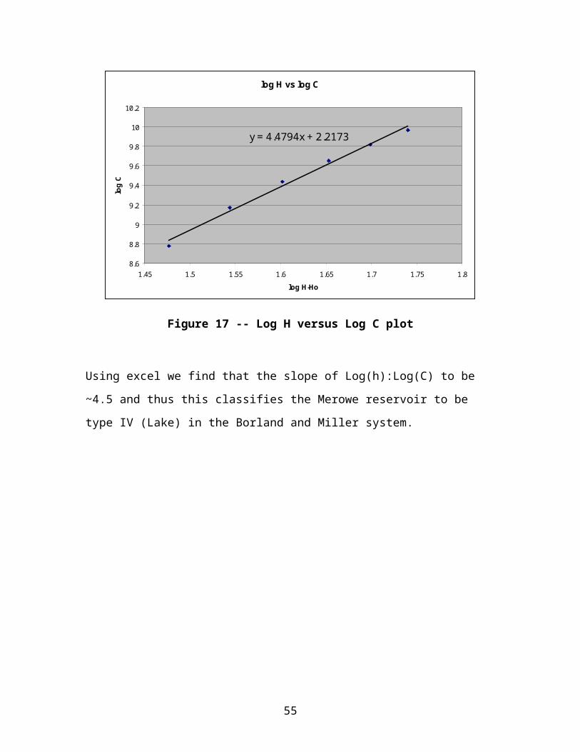
where HO is the lowest elevation of the reservoir bed and α and M are coefficients. The coefficient M is derived by graphing log(C) versus log(H) and taking the mean of the slope.

log H vs log C

y = 4.4794x + 2.2173

8.6

8.8

9

9.2

9.4

9.6

9.8

10

10.2

1.45 1.5 1.55 1.6 1.65 1.7 1.75 1.8

log H-Ho

log

C

Figure 17 -- Log H versus Log C plot

Using excel we find that the slope of Log(h):Log(C) to be ~4.5 and thus this classifies the Merowe reservoir to be type IV (Lake) in the Borland and Miller system.

45

Figure 18 – Location of the Sediment Deposits

Next, we take ratio of the differences of both the M.O.L (Mean Operating Level = 290 m) versus the HO (240m) and the PowerIntake (280m) level versus HO. This gives us the percentage of total depth of reservoir, which we can find the percentage of all deposit that is below H. Thus, we see that given percentage of total depth of reservoir to be 80%, we find that the percent of sediment that will be deposited in the dead space to be 65%. Therefore, approximately 65% of the sediment will be deposited in the dead space and 35% in the active.

3) How long is the economic life?

The economic life of a hydropower dam can be determined with a few assumptions. The way that we will define the economic end of the dam will be when the sediment level reaches the intake for the

46

power turbines (280m) with a corresponding reservoir of 7.31 x 1011 m3. This is the critical point in which sediments can only be deposited into the active storage area of the dam. For the first round calculation, which gives a rate of 67.6 x 106 m3/yr of loss storage, the economic life of this reservoir is estimated to be 40 years. However, since this method did not take into account the change in trapping efficiency as the capacity of the reservoir decreased and , more accurate estimations can be obtained using the iterative method.

Furthermore, we must take into account a probable operating parameter. Namely, the flushing of the high sediment loaded flow months of July-August through which accounts for approximately 40% of the annual total suspended load. Hence, the annual average flow rate minus the flow during the July-August months amounts to 44 billion m3/yr. The following scenarios in Table 6 are done to give an appropriate range of the economic life of the project.

Table 6. Economic Life scenarios – The scenarios vary flow rates, which adjust for flushing during the high sediment laded flood months of July-Aug., represents the range of total suspended load, and varies bed load between 5% and 15%

Scenarios Flow Rate (I)Suspended Load (QC)

Estimated Bed Load

Economic Life

144 billion

m3/yr30 million 5% 350 yrs

263.7 billion

m3/yr50 million 15% 205 yrs

3 44 billion 77 million 5% 105 yrs

47

m3/yr

463.7 billion

m3/yr158 million 15% 65 yrs

544 billion

m3/yr137 million 5% 70 yrs

663.7 billion

m3/yr228 million 15% 45 yrs

**See Appendix C for excel calculations for each individual scenario.

4) What things can be done to improve the situation?

The following are available methods, both their advantages and disadvantages, to deal with the sedimentation:

1) Trapping2) Sluicing3) Dredging4) Operating Parameters

1) Trapping

Smaller subsidiary dams can be built in the upper parts of the catchment system to catch sediment before it reaches the reservoir. A cost benefit analysis should be done to see if the cost per m3 of the trap volume is less than the cost per m3 of the volume being protected in the main reservoir.

2) Sluicing

48

The Merowe dam has been outfitted with low-level outlets to provide high-velocity flushing. It is hoped that these times of flushing will take large amounts of sediment out of the reservoir. However, this method is limited to a local area and not the entire reservoir due to the fact that the induced current will drop decrease in velocity the farther it is from the gates. Thus, a level of the flow will be reached that is lower than that need to mobilize the sediment.

3) Dredging

The option of dredging is not as feasible in large dams as the others due to two reasons: 1) reallocation of large amounts of sediment and 2) the cost of operation. Thus, dredging can be useful to extend the life of a reservoir when its dead storage is nearly full to lower the sediment levels around the intakes.

4) Operating Parameters

One major way of reducing the trapping efficiency of the Merowe dam is to mimic an operating parameter that is effective at Roseires. At Roseires, the reservoir level is kept low at the beginning of the flood season to allow the rising leg of the hydrograph to pass through the low level outlets. This flushing period caries most of the suspended sediment through the reservoir. The retention of water is only done on the lowering leg of the hydrograph in which the concentration of sediments in the water is significantly lower.

49

The Impacts of Dams and Reservoirs on Public Health

Health Impact of Merowe Dam

According to the Kuwait fund, the Merowe Dam project is as much about hope and development as it is about economics and power generation. In order to be a proper, responsible development project, it is crucial that the Dam does not worsen the condition of the Sudanese people. Therefore, the dam planning process should include measures that ensure that the public health in the Merowe region does not decline as a result of the dam. Unfortunately, it appears as though public health has received very little attention in the design of the Merowe Dam. I would like to discuss several diseases that are likely to increase due to the dam, as well as measures that can be taken to mitigate these negative health effects. (Sadeqi, 2004)

According to a health impact analysis conducted by Blue Nile Associates, the Merowe Dam Project will have 27 major health impacts, 20 of which are negative. The three greatest positive impacts will be reductions in river blindness, diarrheal diseases, and malnutrition. The major negative health impacts include threats or increases in Rift Valley Fever, AIDS, and increased transmission of malaria, schistosomiasis, and river blindness both in the resettled population and around the reservoir. (Jobin, 1999)

These impacts vary in terms of their severity, and timescales; some impacts will only be a concern during the construction of the dam, while others will be more long term. This paper will focus on

50

four diseases: malaria, bilharzias, river blindness and Rift Valley fever. All four are transmitted by vectors species, and all are present in Sudan, making it likely that the increase in vector habitat created by the reservoir will greatly increase the prevalence of the disease.

Those in greatest risk are the 50,000 people who will have to be relocated. These people live in settlements along the banks of the river that will be submerged by the reservoir. Although I did not have any information about where these families will be relocated to, it is probably a safe assumption to say that they will be placed in new villages on the banks of the reservoir. They will therefore be in contact with disease vectors living in and around the reservoir.Health Issues Involving Water

Health issues involving water can be broken into four categories: Waterborne, water-based, water-related, and water-washed illnesses. Water-borne illnesses are those caused by consuming water contaminated by human, animal, or chemical wastes. These diseases are especially prevalent in areas lacking access to adequate sanitation facilities, and include diarrhea, cholera and typhoid. Water-based illnesses are caused by parasites that spend at least part of their life cycles in water. These include guinea worm and schistosomiasis. Water-related illnesses are those transmitted by vectors that live and breed in or around water. Vectors are insects or animals that carry and transmit parasites between infected people or animals. This category of disease includes Malaria, transmitted by mosquitoes. Water-washed illnesses are those that can be prevented through more frequent hand-washing and bathing, including trachoma and river blindness. ( Hinrichsen, 1997 & Jobin, 1999)

The main negative public health impacts associated with reservoirs fall into the categories of water-based and water-related

51

diseases. The reservoirs formed by dams provide large areas of stagnant water ideal in which parasites and vectors can breed. Irrigation canals and drainage network also provide habitats for vector species throughout the farming land. Also, dams provide a steady source of water, sustaining organisms that may have otherwise perished during the dry season. (Jobin, 1999) The greatest health threats come from diseases endemic to the region. Careful planning regarding the provision of sanitation facilities to resettled populations removes a large part of the risk of waterborne diseases. Water-washed diseases should, if anything, decrease with the introduction of a dam because the amount of water available to people will either stay the same or increase.

Background on Diseases

Malaria

Malaria is a transmitted between humans by female Anopheles mosquitoes. It is caused by the single-celled protozoa Plasmodium. There are four strains of Plasmodium, the most serious being P. falciparum, which can be fatal, and P. vivax, which can spread into temperature areas. All four types of the parasite are found in Africa, with P. falciparum being the most common (Jobin , 1999). While the disease used to be widespread, it has been eradicated from most temperate regions and is now found mainly across tropical and sub-tropical regions worldwide. Every year, Malaria causes over 300 million acute illnesses and one million deaths worldwide, 90% of which the casualties are young children in Sub-Saharan Africa. The disease also poses an elevated risk to pregnant women. (RBM Malaria Infosheet )

52

The parasite is transmitted to humans during a blood meal of an infected Anopheles mosquito, migrating to the humans’ liver and red blood cells. Symptoms, which appear 8 to 30 days after transmission, include fever, headache, vomiting and muscle ache. The parasite’s cycles of multiplication and destruction of red blood cells is often reflected by cycles of fever, shaking chills and drenching sweats. This process of destroying red blood cells leads to anemia. The infected red blood cells can block the blood supply to the brain or other organs and be fatal. (TDR Malaria) People living in malaria endemic areas acquire some immunity to the disease and become carriers of the disease, posing a threat to people from non-endemic areas.

Infections must be detected based on symptoms and, when possible, a microscopic diagnosis, and promptly treated using locally effective drugs. The malaria parasite is quick to develop resistant to drugs and insecticides, so the effectiveness of these drugs must be evaluated regularly.

Schistosomiasis

Schistosomiasis, also known has bilharzia, is caused by the Schistosoma fluke and is transmitted by snails. There are two types of the disease: urinary schistosomiasis, caused by S. haematobium, and intestinal schistosomiasis, caused by S. mansoni, S. japolicum, and S. mekongi. Infected snails release the parasites in the cercariae larval form, which enter humans in the water through their skin. Adult male and female schistosomes live in human blood vessels, and the female releases eggs. Some of the eggs are passed out in the infected person’s urine or faeces, depending on whether it is the urinary or intestinal form of the disease. If this infected urine or feces comes in contact with water with snails, the eggs will enter the snails perpetuating the cycle of the disease. The rest of the eggs are

53

implanted in the human’s tissues causing immune reactions. (TDR Schistosomiasis )

The main symptom of urinary schistosomiasis is painful urination with blood. This is due to damage caused to the urinary tract, and can lead to bladder cancer if the disease is allowed to advance. Intestinal schistosomiasis causes swelling of the liver and spleen and hypertension of abdominal blood vessels. The immune response to the eggs damages the intestine by forming fibrotic lesions. Bleeding from the abdominal vessels, which leads to bloody stools, can be fatal. People with the disease become weak and their organs can be impaired. This disease is especially dangerous to children. People in frequent contact with water are most likely to acquire schistosomiasis. A study comparing the prevalence of schistosomiasis by occupation in the Nile Delta in 1960 found that farmers, fishermen, and boatmen all had greater than 50% prevalence of the disease, while the prevalence for the total population was only 36%. (Jobin, 1999)

Urinary schistosomiasis was introduced to northern Sudan by Egyptian labourers in 1919. Both types of the disease are now common throughout Sudan. Downstream from Khartoum, areas with pumped irrigation systems have schistosomiasis prevalence below 50%, and areas without pumped irrigation have less than 10% prevalence. This prevalence is expected to increase dramatically as irrigation intensity increases, encouraging growth of the snail population. (Jobin, 1999)

Schistosomiasis is diagnosed by urine filtration and fecal smears, as well as antigen or antibody detection tests. The disease is treated by a single dose of praziquantel for all species, or of oxamniquine for S. mansoni only. Prevention methods for the disease include targeted snail control, provision of safe water supply and sanitation, and health education. (Jobin, 1999)

54

River Blindness

River blindness, or Onchocerciasis, is caused by a parasitic worm, Onchocerca volculus. The worm larvae are transmitted between humans through the bite of infected blackflies. The larvae lodge in nodules they create beneath the human’s skin. Once mature, the worms mate, producing up to a thousand eggs a day. The eggs develop into microfilariae and migrate in the skin tissue where they eventually die, causing skin rashes, lesions, itching and skin depigmentation. If the microfilariae reach the host’s eyes, they can cause blindness. The worms can live in humans for up to 14 years. (TDR Onchocerciasis )

The disease can be safely and effectively treated by a drug developed by Merck & Co. Inc., taken once a year.11 Blackflies breed in fast moving water. The Blue Nile Associates analysis predicted an overall decrease in river blindness because the dam and the reservoir will destroy most of the breeding sites. However, the rapid water on the dam spillways could cause a localized increase in the disease. (Jobin, 1999)

Rift Valley Fever

Rift Valley Fever is a highly lethal hemorrhagic viral disease that occurs after filling a reservoir either for the first time or after a long drought. It is believed that ticks and mosquitoes transmit the virus from sheep and cattle to humans. This disease is especially of concern at the Merowe Dam because two epidemics occurred at the Aswan Dam in Egypt, also on the Nile River. These outbreaks were both devastating, each one killing hundreds of people. There were also three epidemics at dams on the Senegal River. Normally, the

55

virus remains within livestock. However when a new reservoir is created, the sudden increase in mosquito habitat causes an explosion in the mosquito population. When these massive numbers of mosquitoes are in close contact with both the infected animals and humans, it is possible for the disease to be transmitted to humans. Because humans normally have so little exposure to the virus, they have no immunity to it and are thus very susceptible to its effects. (Jobin, 1999)

Mitigating Health Effects

Malaria

The creation of a large reservoir on the Nile River will increase the potential habitat for two species of Malaria-carrying mosquitoes. The first type is the Anopheles funestus vector, which breeds in the illuminated shoreline surrounding reservoirs. The illuminated shoreline is the inner perimeter of the reservoir that is reached by sunlight. The depth, and therefore the area, of the illuminated shoreline depend on the turbidity of the water, and can range between 0.1 and 2 meters. The intersection of the plants and the water surface provides habitat for mosquitoes. A. funestus mosquitoes breed in the illuminated shoreline year round. The area of illuminated shoreline for light penetration depths of 0.1 meter and 2 meters were calculated for the maximum and minimum water levels using the ArcGis Spatial Analyst tool.

Table 7. Illuminated shoreline calculations

Water elevation [m]

light penetration

[m]

Illuminated

shoreline

56

[km^2]

2960.1 2.442 47.11

2900.1 2.012 38.90

The other type of mosquito, Anopheles gambiae, breeds in small, temporary pools of water. These pools occur naturally during the rainy season, as irregular surfaces on the land are filled with water. Such pools usually do not occur during the dry season, as there is not enough rain to fill and maintain them. However, the addition of a reservoir provides abundant pools during the dry seasons because they are left behind as the reservoir recedes.

The drawdown area, which is the area between the maximum and minimum water levels, is shown in Figure 19, and is represented by the spotted region. The area of drawdown was computed using the Surface Analyst tool in ArcGis. The result is a drawdown area of 129 km2.

Drawdown area = Surface area of reservoir at 296 m – Surface area of reservoir at 290 m (1)

57

Figure 19 – Mosquito Habitat & Flight Range

58

Mosquitoes can fly up to 15 km from their breeding ground, but most often remain within 5 km. This flight range is also shown in Figure 19. Caleb King’s study of Malaria transmission in Senegal found the density of mosquitoes to be linearly proportional to the distance from their breeding ground (King, 1996). He developed empirical mosquito density factors as a function of distance that can be multiplied to the breeding areas to give the mosquito density per square kilometer. The mosquito density is then divided by the population density to give a ration of mosquitoes to humans. I calculated the population density to be the number of people to be displaced by the reservoir by the area of the reservoir, giving 77.4 persons/km2. This is a very rough estimate; in order to achieve a better estimate, I would need actual population data. These densities can be used to find the vectorial capacity (VC) of the mosquitoes. This quantity represents the number of potentially infective bites that will result from each infected person, per unit time.

VC=ma2pn/-logep (2) Where m is the mosquito to human ratio

a is the man-biting-parameter, which is the number of bites on man one mosquito will take in a day

p is the daily survival probability of the mosquito vectorsn is the incubation period of the vector in days.

The values for a, p and n can be measured in the field. Because we did not have this data for the Merowe region, I used the values used by King in Senegal: a is 0.45 for A. gambiae and 0.485 for A. funestus, p is 0.819, and n is 10 days.

59

Table 8. Mosquito Model Parameters

density

factor

breeding area (km2)

m (mosquito/hum

an)A VC

A. funestus

0-5 km0.172

2.44 – 47.11

0.005 - 0.0100.48

5

1.8x10-3 - 3.8x10-3

0-15 km0.101 0.003 - 0.06

1.1x10-3 - 2.2x10-2

A. gambiae0-5 km 1.766

1292.94

0.450.93

0-15 km 1.056 1.76 0.56

The vector capacities can be used to estimate the transmission of malaria according to the Garki Model. The Garki equation depends on the proportion of the population with malaria, and is time dependant. Although I lacked the necessary information to conduct this part of the analysis, we can see that the Garki equation can be very useful in predicting malaria prevalence. Based on the vector capacity alone, it appears as though the A. gambiae mosquitoes will be more important in the transmission of malaria than A. funestus.

60

In any case, in incidence of Malaria can be greatly reduced in the communities surrounding the reservoirs by preventing mosquito-to-human contact. Window screens in homes and mosquito netting over beds can greatly reduce mosquito bites, especially at night. Insecticides can be applied to the temporary pools or the reservoir itself to control the mosquito population. Great care must be taken to avoid having humans come in contact with harmful levels of these chemicals, whether through ingestion, inhalation, or dermal exposure. Mosquitoes are often quick to develop resistance against insecticides. The efficacy of the insecticides must therefore be continually monitored, and alternate control methods must be prepared for when the existing method fails. Some species of birds and fish are known for being effective predators of mosquitoes. If any such species are native to the Merowe region, they could be introduced to the reservoir as a form of biological control. Non-native species might also be transferable, but this requires careful ecological analysis to ensure that they do not harm existing ecosystems. Plants growing in the illuminated shoreline can be removed manually or chemically to reduce the A. funestus habitat.

Schistosomiasis

Like the A. funestus mosquito, snails that transmit schistosomiasis live in the illuminated shore zone. This means that control methods for the snails are similar to those of the mosquitoes; mulluscicides, natural predators, and destruction of habitat can all be used against the snail. There is an important difference between schistosomiasis and the other diseases we are concerned about. Unlike the other diseases, which are transmitted between people through vector bites, the snail itself does not infect people. People

61

become infected by coming in direct contact with water containing the parasite. Although this can happen by ingesting the water, the worm also enters humans through the skin. People who come in regular contact with water such as irrigation workers or fishermen should be aware of this threat, and be encouraged to do things such as wear waterproof shoes, pants and gloves. Provision of piped water in resettled households can eliminate the risk pathway of women and children being infected as they go to the reservoir to do their washing or to fetch water.

A preventable part of the schistosome life-cycle is its reintroduction into a water body through contaminated urine or feces. Resettled communities should also be provided with sanitation facilities in order to break this link. Both the piped water supply and the sanitation services will do much more for the communities than just reduce the risk of schistosomiasis. Both are important development goals. They will reduce diarrhea and other water related diseases, facilitate household chores, and greatly improve quality of life. However, neither can be effective without community participation and education; this should also be included as part of the Merowe Dam project.

River Blindness

62

River blindness is a water-washed illness, which means that access to abundant water for washing will reduce the threat of contracting the disease. This stresses the importance of providing relocated families with an adequate water supply. According the World Health Organization, 20 liters per capita per day is the minimum amount of water needed for survival. Ideally, households would be provided with closer to 100 liters per capita per day.

Black flies breed in fast moving water. In our case, the concern is that they will breed in the dam’s spillway. It is possible to control the black fly population by stopping all flow through the dam’s turbines, spillway and sluices for two days at a time every two weeks during the rainy season (July-September). Integrating this into the model, we see the impact it has on power generation:

Table 9. Power Generation

Annual Power Generated (watts)

Percent power reductionnormal

with RB control

Var 12.05E+

11 1.96E+11 4.39

Var 21.99E+

11 1.89E+11 5.03

Var 31.87E+

11 1.77E+11 5.35

Although the overall power loss is not very large, we must also consider the implications of having days where no power is generated. The following figure shows the output graphs when the River Blindness controls are applied to Variation 2. The upward spikes in

63

the volume, height and area graphs correspond to the increase in water caused by the two days worth of water kept within the reservoir. If the power system can sustain itself during the two-day periods of power shutoff, it could very well be worthwhile to implement this into the model’s operating parameters.

Figure 20 – Output for Variation 2 of the model using River Blindness control

Rift Valley Fever

Since Rift Valley fever has been known to occur in large reservoirs on the Nile, great precautions must be taken to prevent the Merowe Dam from causing another epidemic. The livestock surrounding the future reservoir area should be thoroughly screened for the disease. If the disease is detected, or if there is reason to

64

believe that potentially infected livestock may enter the area, the livestock should be vaccinated against the disease. Another option would be to remove all the animals from the area during the initial reservoir filling period. Perhaps people owning animals could be provided with some temporary grazing land and caretakers outside of the mosquitoes’ reach. Or the animals can be purchased by the government for a price great enough to sustain the families until livestock can be reintroduced into the area. These animals can be sold in other parts of the country, either as livestock or as meat.

When an animal is infected, its milk and flesh become contaminated. If an outbreak does occur, all animals in the Merowe region should be quarantined, and their meat and milk should not be eaten. Humans can contract the disease while handling the animals. Everyone involved in the handling or slaughter of livestock should be made aware of the risk and be encouraged to wear long sleeved shirts and cover themselves as much as possible. Unfortunately there is no vaccine for humans at risk of contracting Rift Valley Fever.

The actions to reduce the mosquito population and their contact with humans described in the malaria section are all relevant and important in reducing the risk of Rift Valley Fever.

In addition to all the prevention mechanisms described above, a treatment plan for infected parties must also be developed. All resettled communities should be within a reasonable distance from a medical facility equipped to test for these and other diseases, and to administer the proper treatment when necessary.

Model Comparisons

In comparing the models, we must remember that there are multiple vectors of concern – the black fly that breeds in the fast moving water of the spillway and other dam outlets, the A. funestus

65

mosquito and the snails that live in the illuminated shoreline, and the A. gambiae mosquito that lives in shallow temporary pools created by the receding reservoir. It is not clear what type of mosquito or other insects transmit Rift Valley Fever. Since the disease is associated both with heavy periods of rain as well as the filling of new reservoirs, it seems as the Rift Valley Fever vectors breed in both the shallow pools and the shoreline.

I have already discussed a simple change to the model to reduce the black fly population, reducing the risk of river blindness. Considering our three models, it is clear that Variation 3, the constant head model, would be ideal for controlling the A. gambiae mosquito, as its habitat would virtually be eliminated. However, the steady water level would provide an ideal habitat for the A. funestus mosquito, as well as the schistosomiasis snails. The relative risk of each species should be compared; if it appears as though A. gambiae will cause more health problems than the other two species, then perhaps the constant head operation parameters should be adopted. However, since schistosomiasis is already very prevalent in many parts of Sudan, I believe that it will be more important to reduce snail habitat by varying the water level.

Decreasing the water level for 0.5 meters can leave snails and mosquito larvae stranded on what used to be the illuminated shoreline. The Pessimistic Model might be the best option for controlling these species, as the drawdown happens so quickly that the vectors will not be able to migrate further into the reservoir. It is not obvious whether Variation 1 or Variation 2 would be better for reducing A. gambiae mosquito density. The fast drawdown in Variation 1 will create a sudden increase in A. gambiae habitat, which will cause an initial increase. However, because all of the pools are formed at around the same time, they should all dry up fairly quickly. Variation 2, on the other hand, creates A. gambiae habitat gradually

66

throughout the dry season. Although the initial increase of the mosquito will be tempered, the habitat will last throughout the season, as new pools are constantly replenishing those that dry out. The models could also be modified to include regular reservoir fluctuations throughout the course of the year.

Because the surface area increases as a quadratic function of height, the vector habitat greatly increases with increasing water elevation. It is therefore desirable to keep the water level as low as possible. Of course, this conflicts with the power generation goals. The next step of this project, if we had more time, would have been to conduct a thorough cost-benefit analysis to determine what water level will balance public health, sedimentation and power generating goals. The goal of public health should be to have no increase in disease, and can be achieved through dam operation, vector control, reduced contact with vector, and treatment of disease.

Future Work

A goal is to better integrate each of the individual sections: effects of climate change, sedimentation, and public health. A thorough cost benefit analysis is a top priority. Not only do the tradition factors of cost need to be assed (i.e. construction, material, labor) but other externalities such as decommissioning the dam, burning fossil fuels instead of generating hydropower, and the environmental cost of added CO2 emissions should all be considered.

The definition of each of the climate scenarios can be modified such that a wetter climate can be defined as a 30% or higher increase in the flow. The definition of a drier climate can be similarly modified.

67

The literature review shows a wide range of Nile flow predictions for future years that are not incorporated into this study. In addition, intermonthly variation of flows and not only the average annual flow can be taken into account to better define the definition of wetter or drier climates. More operating parameters, such as one that tries to keep hydropower generation constant throughout the year, can be tested with each climate scenario.

More information about the population of the Merowe region would greatly enhance the public health analysis. The size and location of current and proposed relocated communities, the prevalence of livestock, and people’s willingness to adapt to proposed behavioral changes are all crucial in formulating strategies to mitigate negative health effects. A greater understanding of disease prevalence in Sudan would allow us to better predict which diseases will cause the greatest problems in the Merowe region. Computer models have been developed for many tropical diseases. A next step would be to apply these models to the Merowe region. Once we have a better idea of our priorities between the various diseases, we can adjust the operating parameters of the model so that the reservoir and the dam provide minimal habitat for disease vectors.

Appendix A: Matlab Code

%%%%%%%%% "The New Model" v1.5 – Combined Version %%%%%%%%%%%%%%%

%% initial conditions

numyears=2; % number of years to simulate

68

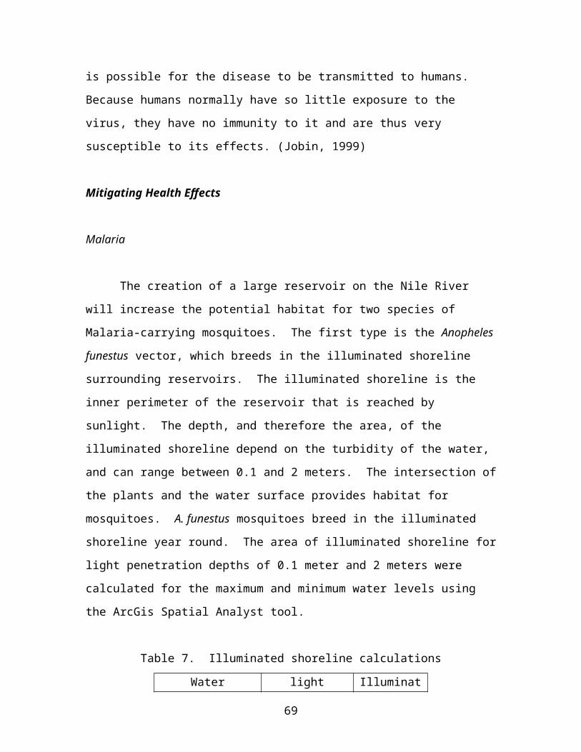
%Dam Propertiesh_target=296; % [m] height above aslh_spill=296; % [m] height of spillway

V_spill=vol_at_h(h_spill); % [m^3]

h_min=290; % [m] height of minh_outlet=240; % ??? [m] height of power plant outflow %Initial Water Volumes & Heightsdelta_V=0; % [m^3] change in volume of entire reservoirh=zeros(numyears*365,1); % Array setup to store daily height of reservoir aslh(1,1)=h_target; % [m] initial height of reservoir level aslh_spillway=0; % [m] initial height of water in spillway channelV_min=vol_at_h(h_min); % [m^3] volume of resevoir at power min heightV=zeros(365*numyears,1); % Array setup to store daily VolumesV_lookback=vol_at_h(h_target); % [m^3] initial volume of reservoir at height of spillwayV_turbine=zeros(365*numyears,1); % [m^3] volume that flows through the turbines at 1 timestep

%Power EquationPower=zeros(365*numyears,1); % [watts] initial poweryearlyP=zeros(numyears,1);E=0.8; % [%] Efficiencygamma=9810; % [kg/m^2/s^2] density of water x gravityturbine_cap=200; % [m^3/s] flow per 1 hydrounitQ_turbine=zeros(365*numyears,1); % [m^3/s] flow through all used turbines

%Timesteptimestep=3600*24; % [s] 1 day of seconds

%Inputs: read from filesload nileflow.txt; % in cubic meters/ second

load evap_2yrs.txt; % in mm/monthevap=evap_2yrs / 30 * 0.001* (6.22 * 10^8) ; % in cubic meters

% find dry season (for variation 2)Avg_Inflow=sum(nileflow)/length(nileflow);dry_ind=find(nileflow<Avg_Inflow); %lists indices of nileflow which have less than average inflowlength_dry=length(dry_ind)/numyears; %gives number of dry days per yaer.

%Loopfor i=1:365*numyears delta_V=nileflow(i)*timestep-evap(i); %Change in Volume V(i)=V_lookback+delta_V; %Volume of entire reservoir at time step (i) %Volume of useable water for Power %%%%%%%%% VARIATION 1 - THE PESSIMISTIC MODEL %%%%%%%%%%%%%% V_useable=V(i) - V_min; % Volume of active storage % %%%%%%%%% VARIATION 2 - THE GRADUAL RELEASE %%%%%%%%%%%% % if nileflow(i)>Avg_Inflow % flood season! use as many turbines as possible

69

% V_useable=V(i) - V_min; % (same as in pessimistic model)% else % dry season - save up!% V_useable = delta_V+(V_spill-V_min)/length_dry; %use inflow, plus rationed storage %volume% end %%%%%%%%% VARIATION 3 - THE CONSTANT HEAD %%%%%%%%%%%%%%% % %only use what comes in!% V_useable=nileflow(i)*timestep - evap(i);% %%%%%%%%%%%%%%%%%%%%%%%%%%%%%%%%%%%%%%%%%%%%%%%% %Determing # of Turbines if V_useable >= turbine_cap*8*timestep % Check to see if useable volume greater than volume of water that can flow through the intake for 1 timestep. num_turbines=8; %Turns all 10 turbines on else %Decide how many turbines to use num_turbines=floor(V_useable/(turbine_cap*timestep)); %The floor command rounds down, so it says how many turbines will run end %Flow of Turbines Q_turbine(i)=num_turbines*turbine_cap; %Flow through turbines V_turbine(i)=Q_turbine(i)*timestep; %Volume that flows through turbines per timestep %height h(i)=h_at_vol2(V(i)); %Head head=h(i)-h_outlet;

%Power Equation Power(i) = E*gamma*Q_turbine(i)*head;

%Reset Volume and height V(i)=V(i)-V_turbine(i); h(i)=h_at_vol2(V(i)); % deal with overflow if needed if V(i) > V_spill a='overflowing'; h(i)=h_spill; %release everything! whee! V(i)=vol_at_h(h_spill); end %have computer remember volume next time around V_lookback=V(i); %area area(i)=area_at_h(h(i)); end

%average yearly power

70

Avg_P=sum(Power)/numyears'average yearly power'sum(Q_turbine)

%plot resultsfiguresubplot(7,1,1),plot(nileflow)title('nile inflow')set (gca,'XTick',0:90:30*12*numyears)set (gca,'XTickLabel',[])

subplot(7,1,2),plot(evap)title('evaporation')set (gca,'XTick',0:90:30*12*numyears)set (gca,'XTickLabel',[])

subplot(7,1,3),plot(V)title('V')set (gca,'XTick',0:90:30*12*numyears)set (gca,'XTickLabel',[])

subplot(7,1,4),plot(h)title('h')set (gca,'XTick',0:90:30*12*numyears)set (gca,'XTickLabel',[])

subplot(7,1,5),plot(area)title('area')set (gca,'XTick',0:90:30*12*numyears)set (gca,'XTickLabel',[])

subplot(7,1,6)plot(Q_turbine/200)title('number of turbines')set (gca,'XTick',0:90:30*12*numyears)set (gca,'XTickLabel',[])

subplot(7,1,7)plot(Power)title('power')set (gca,'XTick',0:90:30*12*numyears)set (gca,'XTickLabel',['Jan'; 'Apr'; 'Jul'; 'Oct'])

Works Cited

Abernethy, Charles L. (1987) Erosion and Sedimentation. Lectures for the International Postgraduate Course in Engineering Hydrology, University College, Galway.

71

American Institute of Physics (API). (2004) “The discovery of global warming: The carbon dioxide greenhouse effect.” May 17, 2004. <http://www.aip.org/history/climate/co2.htm#L_0242>

American Institute of Physics (API). (2004) “1955-65: Establishment of Atmospheric General Circulation Modeling.” March 8, 2004 <http://www.aip.org/history/sloan/gcm/1955_65.html>

Arab Fund. (2003) “The Republic of Sudan: Merowe Dam.” <http://www.arabfund.org/Project/proj422.htm>

BBC News. (2002) “Sudan plans Nile dam.” February, 6, 2004. <http://news.bbc.co.uk/2/low/business/2231464.stm>

Conway, D. and Hulme, M. 1996. The impacts of climate variability and future climate change in the Nile basin on water resources in Egypt. Water Resources Development 12: 277-296.

Davis, J. Overheads for Class Session 2, 11.497 Water and Sanitation Infrastructure Planning in Developing Countries, MIT, January 2004.

D.J. Stanley and J.G. Wingerath. (1996) Nile Sediment Dispersal Altered by the Aswan High Dam: the Kaolinite Trace. Marine Geology 133: 1-9.

Eltahir, Elfatih A. B. El Nino and the natural variability in the flow of the Nile River. Water Resources Research 32(1): 131-137.

Eltahir, Elfatih A. B. & Guiling Wang. Nilometers, El Nino, and Climate Variability. Geophysical Research Letters 26(4): 489-492.

El Moushid, B. E. F., El Awad, O. M. A. & Ahmed, S. E. (1997) Environmental effect of the Blue Nile sediment on reservoirs and irrigation canals. In: 5th Nile 2002 Conf. (Addis Abada).

“Ethiopia.” (2004)  Encyclopædia Britannica. Encyclopædia Britannica Online.3 May 2004  <http://www.search.eb.com/eb/article?eu=114672>.

Hassan, Fekri A. Climatic change, Nile floods and civilization. 1998. Nature and Resources 34(2): 34-40.

Hinrichsen, D., Robey, B., and Upadhyay, U.D. Solutions for a Water-Short World. Population Reports, Series M, No. 14. Baltimore: Johns Hopkins School of Public Health, Population Information Program, December 1997.

72

Hulme, M. 1994. Global climate change and the Nile basin. In The Nile: Sharing a scarce resource, an historical and technical review of water management and of economical and legal issues. Howell, P.P. and J.A. Allan, eds. Cambridge University Press. 408 pp.

Hulme, M., Doherty, R.M., Ngara, T., New, M.G., and D. Lister. 2001. African climate change: 1900-2100. Climate Research 17: 145-168.

Hurst, Black and Simaika. (1978) The Nile Basin, Vol. XI. Egyptian Government Press, Ciaro.

Intergovernmental Panel on Climate Change. McCarthy, James J. et al. Eds. 2001a. Climate Change 2001: Impacts, adaptation, and vulnerability. Contribution of Working Group II to the Third Assessment Report of the IPCC. Cambridge University Press. 1032 pp.

Intergovernmental Panel on Climate Change. Watson, Robert T. and the Core Writing Team. 2001b. Climate change 2001: Synthesis report. Contribution of Working Groups I, II, and III to the Third Assessment Report of the IPCC. Cambridge University Press. 397 pp.

Jobin, W. Dams and Disease.  London: E & FN Spoon, 1999.

Johns, T.C., Gregory, J.M., Ingram, W.J., Johnson, C.E., Jones, A., Lowe, J.A., Mitchell, J.F.B., Roberts, D.L., Sexton, D.M.H., Stevenson, D.S., Tett, S.F.B., and Woodage, M.J. 2003. Anthropogenic climate change for 1860 to 2100 simulated with the HadCM3 model under updated emissions scenarios. Climate Dynamics 20: 583-612.

King, Caleb. “The Incorporation of Health Concerns into African River Basin Planning: A Case Study Based on the Senegal River Basin.” MIT, 1996.

Krom, Stanley, Cliff, and Woodward. (2002) Nile River sediment fluctuations over the past 7000 yr and their key role in sapropel development. Geology. 30 (1): 71-74.

Lahmeyer International. 2001. Merowe Dam Project: Project assessment report. Prepared for Republic of the Sudan Ministry of Irrigation and Water Resources.

M. Gamal Mostafa. (1981) Sediment Processes in the Nile River. Water Master Plan. UNDP Technical Report 12.

73

Mamdouh Shahin. Hydrology of the Nile Basin. Amsterdam: Elsevier, 1985.

Merowe Dam Design. Data from Stage I studies.

Ministry of Irrigation, Government of the Democratic Republic of the Sudan. 1979. Nile Waters Study, Volume 1, Main Report.

National Corporation for Antiques and Museums (NCAM). (2004) “Merowe Dam Archaeological Salvage Project (MDASP).” April, 10, 2004 <http://www.sudachrs.org.uk/Appeal.doc>

Ogunbiyi, Constantine and Simon Norris. (2003) “Fighting Chance.” May, 17, 2004. <http://www.cadwalader.com/assets/article/NorisOgunbiyi090103_compact.pdf>

Ribot, Jesse C., Magalhaes, Antonio R. and Stahis S. Panagides. Eds. 1996. Climate variability, climate change and social vulnerability in the semi-arid and tropics. Cambridge University Press. 175 pp.w

Roll Back Malaria (RBM). (2004) Malaria Infosheet, Geneva: Roll Back Malaria, World Health Organization. March 4, 2004. <www.rbm.who.int>

Sene, K.J., Tate, E.L. and Farquharson, F.A.K. 2001. Sensitivity studies of the impacts of climate change on White Nile flows. Climatic Change 50: 177-208.

The Special Programme for Research and Training in Tropical Diseases (TDR). Malaria. March 5, 2004 <www.who.int/tdr/diseases/malaria/diseaseinfo.htm>

The Special Programme for Research and Training in Tropical Diseases (TDR). (2004) Onchocerciasis. March 5, 2004 <www.who.int/tdr/diseases/oncho/diseaseinfo.htm>

The Special Programme for Research and Training in Tropical Diseases (TDR). (2004) Schistosomiasis. March 5, 2004 <www.who.int/tdr/diseases/schisto/diseaseinfo.htm>

Strzepek, Kenneth M. and David N. Yates. 2000. Responses and thresholds of the Egyptian economy to climate change impacts on the water resources of the Nile River. Climatic Change 46: 339-356.

74

Strzepek, K., Onyeji, C., Saleh, M., and Yates, D. 1995. As assessment of integrated climate change impacts on Egypt. In K. Strzepek and J. Smith (eds.), As Climate Changes: International Impacts and Implications. Cambridge University Press, Cambridge: 57-91.

Sudan Tribune. (2003) “Arab Fund helps finance electricity, road projects in Sudan.” February, 6, 2004. <http://www.sudantribune.com/article_impr.php3?id_article=1550>

Sutcliffe, J.V. & Y. P. Parks. The Hydrology of the Nile. Wallingford, UK: International Association of Hydrological Sciences, 1999.

V. D. Novozhenin and A. M. Lapshin. (2000) Exploitation of Water and Hydropower Resources of the Nile. Hydrotechnical Construction, 24(8-9): 460.

Vito A. Vanoni. (1975) Sedimentation Engineering. American Society of Civil Engineers. pg. 1

World Economic Forum. (2003) “Renewable energy powering Africa.” May, 17, 2004. <http://www.weforum.org/site/knowledgenavigator.nsf/Content/Renewable%20Energy%20Powering%20Africa_2003?open&event_id=>

Yates, David N. and Kenneth M. Strzepek. 1998a. An assessment of integrated climate change impacts on the agricultural economy of Egypt. Climatic Change 38:261-287.

Yates, David N. and Kenneth M. Strzepek. 1998b. Modeling the Nile basin under climatic change. Journal of Hydrologic Engineering 3(2): 98-108.

75