1. Introduction 10 - therackonline.com€¦ · 1. Introduction 10 - therackonline.com ... Introduction)

COMPACTNESS OF SCALAR-FLAT CONFORMAL METRICS
ON LOW-DIMENSIONAL MANIFOLDS
WITH CONSTANT MEAN CURVATURE ON BOUNDARY
SEUNGHYEOK KIM, MONICA MUSSO, AND JUNCHENG WEI
Abstract. We concern C2-compactness of the solution set of the boundary Yamabe prob-lem on smooth compact Riemannian manifolds with boundary provided that their dimen-sions are 4, 5 or 6. By conducting a quantitative analysis of a linear equation associated tothe problem, we prove that the trace-free second fundamental form must vanish at possibleblow-up points of a sequence of blowing-up solutions. Together with the positive mass theo-rem, we conclude the C2-compactness holds for all 4-manifolds (which may be non-umbilic).For 5- and 6-manifolds, we also prove that the C2-compactness is true if the trace-free secondfundamental form on the boundary never vanishes.
1. Introduction
Let (M, g) be an N -dimensional (N ≥ 3) smooth compact Riemannian manifold withboundary ∂M . Let also ∆g be the Laplace-Beltrami operator on M , R[g] the scalar curvatureon M , ν the inward normal vector to ∂M , and H[g] be the mean curvature of ∂M . In [21],Escobar asked if (M, g) can be conformally deformed to a scalar-flat manifold with boundaryof constant mean curvature. This problem, which we will call the boundary Yamabe problem,can be understood as a generalization of the Riemann mapping theorem and is equivalentto finding a positive smooth solution to a nonlinear boundary value problem with criticalexponent {
LgU = 0 in M,
BgU = Q(M,∂M)UNN−2 on ∂M.
(1.1)
Here Lg is the conformal Laplacian and Bg is the associated conformal boundary operatordefined as
Lg = −∆g +N − 2
4(N − 1)R[g] and Bg = − ∂
∂ν+N − 2
2H[g],
and Q(M,∂M) is a constant whose sign is determined by the conformal structure of M .Weak solutions to (1.1) correspond to critical points of the functional
Q(U) =
∫M (|∇gU |2g + N−2
4(N−1)R[g]U2)dvg +∫∂M H[g]U2dvh
(∫∂M |U |
2(N−1)N−2 dvh)
N−2N−1
defined for an element U in the Sobolev space H1(M) with U 6= 0 on ∂M , where∇g representsthe gradient on (M, g), h is the restriction of the metric g on ∂M , and dvg and dvh are thevolume form on M and on ∂M , respectively. Escobar [21] proved that the Sobolev quotient
Q(M,∂M) = inf{Q(U) : U ∈ H1(M), U 6= 0 on ∂M
}attains its minimizer if Q(M,∂M) < Q(BN , ∂BN ) where the unit ball BN = {x ∈ RN : |x| <1} is endowed with the Euclidean metric. This is analogous to the observation of Aubin [7]for the classical Yamabe problem.
Date: June 4, 2019.2010 Mathematics Subject Classification. 35B40, 35J65, 35R01, 53A30, 53C21.Key words and phrases. Boundary Yamabe problem, Compactness, Blow-up analysis.
1

2 SEUNGHYEOK KIM, MONICA MUSSO, AND JUNCHENG WEI
Thanks to the effort of several researchers, the existence of a solution to (1.1) is now well-established: Escobar [21, 23], Marques [41, 42], Almaraz [1] and Chen [11] found a minimizerof the functional Q for almost all manifolds. By applying the barycenter technique of Bahriand Coron, Mayer and Ndiaye [33] covered all the remaining cases. Regularity property of(1.1) was investigated by Cherrier [12].
Concerning multiplicity of solutions to (1.1), the only interesting case is when Q(M,∂M) >0. If Q(M,∂M) < 0, the conformal covariance of the operators Lg and Bg shows that (1.1)has only one solution. If Q(M,∂M) = 0, it is a linear equation and its solution is uniqueup to positive multiplicative constants. On the other hand, the case that M is conformallyequivalent to the unit ball BN (so that Q(M,∂M) = Q(BN , ∂BN ) > 0) is special, and thesolution set of (1.1) was completely classified thanks to the works of Escobar [20] and Li andZhu [38]; see Subsection 2.2.
In about two decades, several results on C2(M)-compactness of the solution set of (1.1)appeared under the assumption that Q(M,∂M) > 0. Felli and Ould Ahmedou [24, 25]deduced compactness results for locally conformally flat manifolds and 3-manifolds providedthat their boundaries are umbilic. Very recently, the umbilicity condition was lifted for 3-manifolds by Almaraz et al. [5]. If the dimension N of the manifold M satisfies N ≥ 7 andthe trace-free second-fundamental form on ∂M does not vanish, the result of Almaraz [2]shows that the C2(M)-compactness continues to hold. If either N > 8 and the Weyl tensorof M never vanishes on ∂M , or N = 8 and the Weyl tensor of ∂M never vanishes on ∂M , theC2(M)-compactness is still true for manifolds with umbilic boundary, as shown by Ghimentiand Micheletti [26].
Compactness results for other boundary Yamabe-type problems can be found in Han andLin [29], Djadli et al. [16, 17], Disconzi and Khuri [15], and so on. By using the compactnessproperty, Cadenas and Sierra [10] also yielded uniqueness of solutions to (1.1) for somemanifolds whose metrics are non-degenerate.
As far as the authors know, compactness results on (1.1) have been known only for mani-folds of dimension N = 3 or N ≥ 7, unless manifolds are locally conformally flat. The mainpurpose of this paper is to treat generic manifolds of dimension N = 4, 5 and 6.
Theorem 1.1. For N = 4, 5, 6, let (M, g) be an N -dimensional smooth compact Riemannianmanifold with boundary ∂M such that Q(M,∂M) > 0 and M is not conformally equivalentto the unit ball BN . If N = 5, 6, we also assume that the trace-free second-fundamental formnever vanishes on ∂M . Then, for any ε0 > 0 small, there exists a constant C > 1 dependingonly on M, g and ε0 such that
C−1 ≤ U ≤ C on M and ‖U‖C2(M) ≤ C
for any solution U ∈ H1(M) to{LgU = 0 in M,
BgU = Q(M,∂M)Up on ∂M(1.2)
with p ∈ [1 + ε0,NN−2 ].
As can be observed in Theorem 1.1, we will deal with a slightly generalized equation (1.2)compared to (1.1). We leave two remarks for the theorem.
Remark 1.2. The key idea of our main theorem is to perform a fine analysis of associatedlinearized equations to (1.2) in order to establish that the trace-free second fundamental formmush vanish at possible blow-up points of a sequence of blowing-up solutions. Interestingly,this process is somehow related to the way that Marques [42] constructed test functions in hisexistence theorem for (1.1) on low-dimensional manifolds with non-umbilic boundary. Indeed,his test functions consist of not only truncated bubbles but also some additive correctionterms. This is a distinctive feature of the boundary Yamabe problem compared with theclassical one.

COMPACTNESS OF SCALAR-FLAT CONFORMAL METRICS 3
We provide some possible settings where our argument can be further applied.
(1) Based on the existence results of Marques [41] and Almaraz [1] for (1.1) on manifoldswith umbilic boundary, we expect that one can lower the threshold dimension 8 inthe aforementioned compactness theorem of Ghimenti and Micheletti [26] to 6.
(2) As a matter of fact, the boundary Yamabe problem can be seen as the special caseof the fractional Yamabe problem where the symbol of the differential operator is thesame as that of the half-Laplacian. In [32], we proved that the solution set of thefractional Yamabe problem is C2-compact on conformal infinities of asymptoticallyhyperbolic manifolds, under the assumptions that the dimension is sufficiently highand the second-fundamental form never vanishes. In view of our existence result [31],we expect that the compactness result holds for conformal infinities of dimension ≥ 4as far as the same geometric condition is maintained.
(3) To examine stability issue under small perturbation of (1.1), Ghimenti et al. [27, 28]constructed blowing-up solutions when the linear perturbation of the mean curvatureon the boundary is strictly positive everywhere; see also Deng et al. [14] where analo-gous results were derived in the setting of the fractional Yamabe problem. In buildingsuitable approximation solutions, they had to analyze an associated linearized equa-tion to (1.1) which is essentially the same as ours. Due to this reason, their resultsrequire some dimensional assumptions. Our method can allow one to treat lower-dimensional cases.
We ask the reader to look at Sections 4 and 5 for more description of our ideas.
Remark 1.3. Our strategy follows the argument in the lecture note [43] of Schoen where heraised the question of C2-compactness of the solution set of the classical Yamabe problemand resolved it for locally conformally flat manifolds. It has been further developed by Li andZhu [39], Druet [18], Marques [40], Li and Zhang [36, 37] and Khuri et al. [30]. Furthermore,Li [34] and Li and Xiong [35] studied compactness results of the Q-curvature problem, whichis the fourth-order analogue of the Yamabe problem.
Once Theorem 1.1 is established, one can deduce the existence of a solution to (1.1) byapplying the standard Leray-Schauder degree argument as in [24, 29]. There should exist thestrong Morse inequality in our framework as in [30, Theorem 1.4].
See also Remark 7.4 where we compare our theorem and the corresponding result [40] for theclassical Yamabe problem.
In [3], Almaraz constructed manifolds with umbilic boundary of dimension N ≥ 25 onwhich the solution set of (1.1) is L∞-unbounded (in particular, C2-noncompact). In view ofthe full compactness result of Khuri et al. [30] and the non-compactness results of Brendle[8] and Brendle and Marques [9] for the classical Yamabe problem, a natural expectation isthat the solution set of (1.1) is C2-compact for all manifolds of dimension N ≤ 24 under thevalidity of the positive mass theorem. However, although Schoen’s arugment in [43] worksin principle (as the previous results and our theorem indicates), achieving this seems a quitedifficult task.
To establish the C2-compactness result for general manifolds of high dimension, we mustprove that the trace-less second fundamental form and the Weyl tensor vanish up to some highorder at each blow-up point. This requires a very accurate pointwise estimate of blowing-upsolutions, which can be achieved only if one has a good understanding of linearized equations.In the analysis on the classical Yamabe problem, Khuri et al. [30] observed that solutions oftheir linearized problems can be written explicitly in the form of rational functions. Unfor-tunately, the boundary Yamabe problem seems not to have a similar property.
On the other hand, we may also need a quite precise control of the Green’s function G ofthe conformal Laplacian with Neumann boundary condition; see (2.17) of its definition. Inour analysis, we only need a rough control of G (described in Lemma 2.4) as in the proof ofthe compactness theorem for 3-dimensional manifolds [5].

4 SEUNGHYEOK KIM, MONICA MUSSO, AND JUNCHENG WEI
The rest of the paper is organized as follows:
- In Section 2, we recall some analytic and geometric tools which we need throughoutthe proof of Theorem 1.1. These include the expansion of the metric in Fermi coor-dinates, definition of the bubbles, a local Pohozaev’s identity and the positive masstheorem on asymptotically flat manifolds with boundary.
- In Section 3, we characterize blow-up points of solutions to (1.2) and provide basicqualitative properties of solutions near blow-up points.
- In Section 4, we study a linearized equation associated to (1.2) arising from the first-order expansion of the metric. In order to treat low-dimensional manifolds, we needto understand its solution more precisely than higher-dimensional cases. For this aim,we decompose the solution into two pieces and analyze them quantitatively. This isthe key part of our idea for the proof. We also perform a refined blow-up analysis.
- In Section 5, we carry out the proof of the vanishing theorem of the trace-free sec-ond fundamental form at any isolated simple blow-up point. This is based on thequantitative analysis of the linearized equation conducted in the previous section.
- In Section 6, employing the vanishing theorem, we prove a local Pohozaev sign con-dition that guarantees that every blow-up point is isolated simple.
- In Section 7, by applying the positive mass theorem, we conclude that the solutionset of (1.2) is C2-compact for all 4-manifolds unless it is conformally equivalent to theunit ball. For 5- or 6-manifolds, we also show that the C2-compactness of the solutionset holds provided that the trace-free second fundamental form on the boundary nevervanishes.
- In Appendix A, we provide technical arguments regarding the two pieces of the solu-tions to the linearized equation to (1.2).
To elucidate our method, we will omit most of the proofs of intermediate results which closelyfollow those of the corresponding ones in similar settings, leaving appropriate referencesinstead.
Notations.
- Let n = N − 1. Moreover, for any x ∈ RN+ = {(x1, · · · , xn, xN ) ∈ RN : xN > 0}, we denote
x = (x1, · · · , xn) ∈ Rn. We often identify x ∈ Rn and (x, 0) ∈ ∂RN+ .
- We will sometimes use ∂a = ∂∂xa
, ∂ab = ∂2
∂xa∂xb, etc.
- Given x ∈ RN+ , x ∈ Rn and r > 0, let BN+ (x, r) be the N -dimensional upper half-ball
centered at x of radius r, and Bn(x, r) the n-dimensional ball centered at x of radius r. Weoften identify Bn(x, r) and ∂BN
+ ((x, 0), r)∩ ∂RN+ . Set ∂IBN+ ((x, 0), r) = ∂BN
+ ((x, 0), r)∩RN+ .
- S represents a surface measure. Its subscript x or x denotes the dependent variables.
- D1,2(RN+ ) is the homogeneous Sobolev space in RN+ defined as
D1,2(RN+ ) ={U ∈ L
2NN−2 (RN+ ) : ∇U ∈ L2(RN+ )
}.
- |Sn−1| is the surface area of the unit (n− 1)-sphere Sn−1.
- The metric h on the boundary ∂M of the Riemannian manifold (M, g) is the restriction ofthe metric g to ∂M .
- For any y ∈ ∂M and r > 0 small, Bg(y, r) and Bh(y, r) stand for the geodesic half-ball on(M, g) and the geodesic ball on (∂M, h), respectively. Also, dg is the distance function on(M, g).
- The Einstein summation convention for repeated indices is adopted throughout the paper.Unless otherwise stated, the indices i, j, k, l, m and s always range over values from 1 to n,while a, b, c and d take values from 1 to N . Also, δab is the Kronecker delta.

COMPACTNESS OF SCALAR-FLAT CONFORMAL METRICS 5
- We denote by Rabcd[g] the full Riemannian curvature tensor on (M, g), by Rab[g] the Riccicurvature tensor on M , and by R[g] the scalar curvature on M . The quantities Rijkl[h],Rij [h] and R[h] are the corresponding curvatures defined on the boundary (∂M, h).
- We write by II[g] the second fundamental form of ∂M , by H[g] = 1nh
ijIIij [g] the meancurvature on ∂M , and by π[g] = II[g] −Hg the trace-free second fundamental form of ∂M .Furthermore, ‖π[g]‖2 = hikhjlπij [g]πkl[g] stands for the square of its norm.
- For an r-tensor T , we write
Symi1···irTi1···ir =1
r!
∑σ∈Sr
Tiσ(1)···iσ(r)
where Sr is the symmetric group over a set of r symbols.
- For a multi-index α = (α1, · · · , αn) ∈ Rn,
|α| =n∑i=1
αi, α! =n∏i=1
αi! and∂
∂xα=
∂α1
∂xα11
· · · ∂αn
∂xαnn. (1.3)
β, β′ and β′′ also denote multi-indices.
- The letter C denotes a generic positive constant that may vary from line to line.
2. Preliminaries
2.1. Metric expansion and conformal coordinates. Fix a point y∗ ∈ ∂M . For anyy ∈ ∂M near y∗, let x = (x1, · · · , xn) ∈ Rn be normal coordinates on ∂M (centered at y∗) ofy. Denote by ν(y) the inward normal vector to ∂M at y. We say that x = (x, xN ) ∈ RN+ isFermi coordinates on M (centered at y∗) of the point expy(xNν(x)) ∈M .
In Lemma 2.2 of Marques [41], the following expansion of the metric g near y∗ was given.
Lemma 2.1. In Fermi coordinates centered at y∗ ∈M , it holds that
gij(x) = δij +Aij(x) +O(|x|4),
giN (x) = 0 and gNN (x) = 1, where
Aij(x) = −2IIij [g]xN −1
3Rikjl[h]xkxl − 2IIij,k[g]xkxN + (−RiNjN [g] + IIis[g]IIsj [g])x2
N
− 1
6Rikjl,m[h]xkxlxm +
(−IIij,kl[g] +
2
3Symij(Riksl[h]IIsj [g])
)xkxlxN
+(−RiNjN,k[g] + 2Symij(IIis,k[g]IIsj [g])
)xkx
2N
+1
6
(−2RiNjN,N [g] + 8Symij(IIis[g]RjNsN [g])
)x3N .
Every tensor in the expansion is evaluated at y∗ and commas denote covariant differentiation.
The next lemma describes the existence of conformal coordinates. Refer to Propositions3.1 and 3.2 of [41].
Lemma 2.2. For given a point y∗ ∈M and an integer κ ≥ 2, there exists a metric g on Mconformal to g such that
det g(x) = 1 +O(|x|κ) (2.1)
in g-Fermi coordinates centered at y∗. In particular,
H[g] = H,i[g] = Rij [h] = 0 and RNN [g] = −‖π[g]‖2 at y∗. (2.2)
Moreover, g can be written as g = ω4
N−2 g for some positive smooth function w on ∂M suchthat w(y∗) = 1 and ∇w(y∗) = 0.

6 SEUNGHYEOK KIM, MONICA MUSSO, AND JUNCHENG WEI
2.2. Bubbles in the Euclidean half-space. Assume that N ≥ 3. For λ > 0 and ξ ∈ Rn,let a bubble Wλ,ξ be a function defined as
Wλ,ξ(x) =λN−2
2
(|x− ξ|2 + (xN + λ)2)N−2
2
for x ∈ RN+ , (2.3)
which is an extremal function of the Sobolev trace inequality D1,2(RN+ ) ↪→ L2(N−1)N−2 (Rn); see
Escobar [19]. According to Li and Zhu [36], any solution to the boundary Yamabe problemon RN+
−∆U = 0 in RN+ ,U > 0 in RN+ ,
− ∂U
∂xN= (N − 2)U
NN−2 on Rn
(2.4)
must be a bubble. Note that a sequence {W 1n,0}n∈N of bubbles exhibits a blow-up phenomenon
as n→∞, and in particular, the family of all bubbles is not L∞(RN+ )-bounded. Furthermore,Davila et al. [13] proved that the solution space of the linear problem
−∆Φ = 0 in RN+ ,
− ∂Φ
∂xN= Nw
2N−2
λ,ξ Φ on Rn,
‖Φ(·, 0)‖L∞(Rn) <∞,
where wλ,ξ(x) = Wλ,ξ(x, 0) on Rn, is spanned by
Z1λ,ξ =
∂Wλ,ξ
∂ξ1, · · · , Znλ,ξ =
∂Wλ,ξ
∂ξnand Z0
λ,ξ = −∂Wλ,ξ
∂λ;
refer also to Lemma 2.1 of [2].
2.3. Conformally invariant equations. Let δ = NN−2 − p ≥ 0. It turns out that it is more
convenient to deal with the following form of the equation{LgU = 0 on M,
BgU = (N − 2)f−δUp on ∂M(2.5)
than (1.2). Indeed, by the conformal covariance property of the operators Lg and Bg, the
metric g = ω4
N−2 g conformal to g and the function U = ω−1U > 0 on M satisfy{LgU = 0 on M,
BgU = (N − 2)f−δUp on ∂M,(2.6)
where f = ωf . Obviously, it is an equation of the same type as (2.5).We will study a sequence {Um}m∈N of solutions to (2.5) with suitable choices of the ex-
ponents p = pm ∈ [1 + ε0,NN−2 ] and δ = δm = N
N−2 − pm, the metric g = gm on M and thesmooth positive function f = fm on ∂M . Although we postpone their specific description toSection 3, we stress that our choices will induce that pm → p0, gm → g0 in C4(M,RN×N )and fm → f0 > 0 in C2(∂M) as m→∞, and g0 is a metric on M .
2.4. Pohozaev’s identity. In the analysis of blowing-up solutions, we shall rely on thefollowing version of local Pohozaev’s identity. For its derivation, see Proposition 3.1 of [2].
Lemma 2.3. Assume that N ≥ 3. Let U ∈ H1(BN+ (0, ρ1)) be a solution to−∆U = Q in BN
+ (0, ρ1),
− ∂U
∂xN+N − 2
2HU = fUp on Bn(0, ρ1)

COMPACTNESS OF SCALAR-FLAT CONFORMAL METRICS 7
where p ∈ [1, NN−2 ], Q ∈ L∞(BN
+ (0, ρ1)) and H, f ∈ C1(Bn(0, ρ1)). For any ρ ∈ (0, ρ1), wedefine
P ′(U, ρ) =
∫∂IB
N+ (0,ρ)
[−(N − 2
2
)U∂U
∂ν− ρ
2|∇U |2 + ρ
∣∣∣∣∂U∂ν∣∣∣∣2]dSx, (2.7)
and
P(U, ρ) = P ′(U, ρ) +ρ
p+ 1
∫∂Bn(0,ρ)
fUp+1dSx (2.8)
where ν is the inward unit normal vector with respect to ∂IBN+ (0, ρ). Then we have
P(U, ρ) = −∫BN+ (0,ρ)
Q
[xa∂aU +
(N − 2
2
)U
]dx
+N − 2
2
∫Bn(0,ρ)
H
[xi∂iU +
(N − 2
2
)U
]Udx
− 1
p+ 1
∫Bn(0,ρ)
xi∂ifUp+1dx+
(N − 1
p+ 1− N − 2
2
)∫Bn(0,ρ)
fUp+1dx
(2.9)
for all ρ ∈ (0, ρ1).
2.5. Positive mass theorem. In [4], Almaraz et al. introduced the mass of N -dimensionalasymptotically flat manifolds with non-compact boundary and proved the associated positivemass theorem provided that either 3 ≤ N ≤ 7, or the manifold is spin and N ≥ 3. In [5],Almaraz et al. used this result to describe the asymptotic behavior of the Green’s function ofthe conformal Laplacian on a smooth compact Riemannian manifold (M, g) with boundaryin terms of the mass.
The version of the positive mass theorem which we will apply in this paper is summarizedin the following lemma. This is a combination of Propositions 3.5 and 3.6, and Section 7 of[5].
Lemma 2.4. For 3 ≤ N ≤ 7, let (M, g) be an N -dimensional smooth compact Riemannianmanifold with boundary which is not conformally equivalent to the unit ball. Fix any y0 ∈M .Suppose that we have the following metric expansion
gab(x) = δab +Aab(x) +O(|x|2d+2), d =
⌊N − 2
2
⌋(2.10)
with
AiN (x) = ANN (x) = 0, Aij(x) = O(|x|d+1), trace(A(x)) = O(|x|2d+2) (2.11)
and ∫∂IB
N+ (0,ρ)
(ρ3−2Nxa∂bAab(x)− 2Nρ1−2NxaxbAab(x)
)dSx = O(ρ) (2.12)
in Fermi coordinates centered at y0.1 Assume also that G is a smooth positive function onM \ {y0} such that
G(x) = |x|2−N + φ(x) (2.13)
in the same coordinates, where φ is a smooth function on M \ {y0} satisfying
φ(x) = O(|x|d+3−N | log |x||) as |x| → 0. (2.14)
Then the manifold (M \ {y0}, G4
N−2 g) is asymptotically flat with the mass m0 and
limρ→0P ′(G, ρ) = − (N − 2)2
8(N − 1)m0 (2.15)
1Estimate (2.12) is needed in the proof of Proposition 3.6 of [5]. Using the symmetry of the tensor Aabwhich we use, we will directly check its validity in Lemma 7.2.

8 SEUNGHYEOK KIM, MONICA MUSSO, AND JUNCHENG WEI
where P ′ is the function defined in (2.7). Furthermore, if
R[G
4N−2 g
]≥ 0 on M \ {y0} and H
[G
4N−2 g
]≥ 0 on ∂M \ {y0}, (2.16)
then m0 > 0 and so the right-hand side of (2.15) is negative.
In particular, we will choose G as the normalized Green’s function Gy0 of the conformalLaplacian with Neumann boundary condition with pole at y0, that is, the solution of
LgGy0(y) = 0 in M,
BgGy0(y) = δy0 on ∂M,
limdg(y,y0)→0
dg(y, y0)N−2Gy0(y) = 1.(2.17)
Here, δy0 is the Dirac measure centered at y0 ∈M . More explanation will be given in Section7.
3. Basic properties of blow-up
3.1. Characterization of blow-up points. We recall the notion of blow-up, isolated blow-up and isolated simple blow-up. By virtue of Proposition 3.2, it is enough to consider whenthe blow-up occurs near a point on the boundary. The version we will use here is identicalto those in [2, 5].
Definition 3.1. Pick a small number ρ1 > 0 such that gm-Fermi coordinates centered at
y ∈ ∂M is well-defined in the closed geodesic half-ball BN+ (y, ρ1) ⊂ M for every m ∈ N and
y ∈ ∂M .
(1) y0 ∈ ∂M is called a blow-up point of a sequence {Um}m∈N in H1(M) if there exists asequence of points {ym}m∈N ⊂ ∂M such that ym is a local maximum of Um|∂M satisfyingthat Um(ym) → ∞ and ym → y0 as m → ∞. For the sake of brevity, we will often say thatym → y0 is a blow-up point of {Um}m∈N.
(2) y0 ∈ ∂M is an isolated blow-up point of {Um}m∈N if y0 is a blow-up point such that
Um(y) ≤ Cdgm(y, ym)− 1pm−1 for any y ∈M \ {ym}, dgm(y, ym) < ρ2
for some C > 0 and ρ2 ∈ (0, ρ1].
(3) Let Um be a weighted spherical average of Um, i.e.,
Um(ρ) = ρ1
pm−1
(∫∂IB
N+ (ym,ρ) Um dSgm∫
∂IBN+ (ym,ρ) dSgm
), ρ ∈ (0, ρ1). (3.1)
We say that an isolated blow-up point y0 of {Um}m∈N is simple if there exists a numberρ3 ∈ (0, ρ2] such that Um possesses exactly one critical point in the interval (0, ρ3) for largem ∈ N.
Hereafter, we always assume that Um ∈ H1(M) is a solution to (2.5) with p = pm, g = gmand fm = 1 for each m ∈ N. For simplicity, we will just say that {Um}m∈N is a sequence ofsolutions to (2.5). We also assume that ym → y0 ∈ ∂M is a blow-up point of {Um}m∈N. Set
Mm = Um(ym) and εm = M−(pm−1)m for each m ∈ N. Obviously, Mm → ∞ and εm → 0 as
m→∞.
Choose a suitable positive smooth function ωm onM so that the metric gm = ω4
N−2m gm onM
satisfies properties depicted in Lemma 2.2 where y∗ is replaced with ym. Then Um = ω−1m Um
is a solution to (2.6) with g = gm and f = fm = ωmfm, and a sequence {gm}m∈N of themetrics converges to a metric g0 in C4(M,RN×N ) as m→∞. We shall often use x ∈ RN+ to
denote gm-Fermi coordinates centered at ym so that Um can be regarded as a function in RN+near the origin.

COMPACTNESS OF SCALAR-FLAT CONFORMAL METRICS 9
3.2. Basic properties of blowing-up solutions. Firstly, we study asymptotic behaviorof a sequence {Um}m∈N of solutions to (2.5) near blow-up points. It can be proved as in e.g.Proposition 1.1 of [29] or Proposition 3.2 of [24].
Proposition 3.2. Assume that N ≥ 3 and p ∈ [1 + ε0,NN−2 ]. Given arbitrary small ε1 > 0
and large R > 0, there are constants C0, C1 > 0 depending only on (MN , g), ε0, ε1 andR such that if U ∈ H1(M) is a solution to (1.2) with the property that maxM U ≥ C0,then N
N−2 − p < ε1 and U |∂M possesses local maxima y01, · · · y0N ∈ ∂M for some integer
N = N (U) ≥ 1, for which the following statements hold:
(1) It is valid that
Bh(y0m1 , ρm1) ∩Bh(y0m2 , ρm2) = ∅ for 1 ≤ m1 6= m2 ≤ N
where ρm = RU(y0m)−(p−1).
(2) For each m = 1, · · · ,N , we have∥∥∥U(y0m)−1U(U(y0m)−(p−1)·
)−W1,0
∥∥∥C2(BN+ (0,2R))
≤ ε1
in g-Fermi coordinates centered in ym.
(3) It holds that
U(y) dh(y, {y01, · · · , y0N })1p−1 ≤ C1 for y ∈M.
Secondly, we discuss behavior of a sequence of solutions {Um}m∈N to (2.5) near isolatedblow-up points. The next lemma can be proved as in e.g. Proposition 1.4 of [29] or Lemma2.6 of [24].
Lemma 3.3. Let ym → y0 ∈ ∂M be an isolated blow-up point of a sequence {Um}m∈N ofsolutions to (2.5). In addition, suppose that {Rm}m∈N and {τm}m∈N are arbitrary sequencesof positive numbers such that Rm →∞ and τm → 0 as m→∞. Then pm → N
N−2 as m→∞,
and {U`}`∈N and {p`}`∈N have subsequences {U`m}m∈N and {p`m}m∈N such that∥∥∥∥ε 1p`m−1
`mU`m (ε`m ·)−W1,0
∥∥∥∥C2(BN+ (0,Rm))
≤ τm (3.2)
in gm-Fermi coordinates centered in ym and Rmε`m → 0 as m→∞.
Therefore, we can select {Rm}m∈N and {U`m}m∈N satisfying (3.2) and Rmε`m → 0. In orderto simplify notations, we will use {Um}m∈N instead of {U`m}m∈N, and so on.
The following result is a simple consequence of Lemma 3.3 with the selection τm =12w1,0(Rm). Its proof is given in Corollary 3.6 of [32].
Corollary 3.4. Suppose that ym → y0 ∈ ∂M is an isolated blow-up point of a sequence{Um}m∈N of solutions to (2.5).
(1) If {Um}m∈N is a sequence of solutions to (2.6) constructed as in Subsection 3.1, then
ym → y0 ∈ ∂M is an isolated blow-up point of {Um}m∈N.
(2) The function Um in (3.1) has exactly one critical point in the interval (0, Rmεm) for largem ∈ N. In particular, if the isolated blow-up point y0 ∈ ∂M of {Um}m∈N is also simple, then
U′m(r) < 0 for all r ∈ [Rmεm, r3); see Definition 3.1 (3).
Thirdly, we examine how a sequence {Um}m∈N of solutions to (2.5) behaves near isolatedsimple blow-up points. See Proposition 4.3 of [2] for its proof.

10 SEUNGHYEOK KIM, MONICA MUSSO, AND JUNCHENG WEI
Proposition 3.5. Assume that N ≥ 3 and ym → y0 ∈ ∂M is an isolated simple blow-up
point of a sequence {Um}m∈N of solutions to (2.5), and {Um}m∈N is a sequence of solutions to(2.6) constructed as in Subsection 3.1. Then there exists C > 0 and ρ4 ∈ (0, ρ3) independentof m ∈ N such that
Mm
∣∣∣∇`Um(x)∣∣∣ ≤ C|x|−(N−2+`) in
{x ∈ RN+ : 0 < |x| ≤ ρ4
}(3.3)
for ` = 0, 1, 2 and
MmUm(x) ≥ C−1Gm(x) in{x ∈ RN+ : Rmεm ≤ |x| ≤ ρ4
}in gm-Fermi coordinate system centered at ym. Here, Gm is the Green’s function satisfying
LgmGm = 0 in BN+ (0, ρ4),
BgmGm = δ0 on Bn(0, ρ4),
Gm = 0 on ∂IBN+ (0, ρ4),
lim|x|→0 |x|N−2Gm(x) = 1,
and δ0 is the Dirac measure centered at 0 ∈ RN+ . Also,
M δmm = M
NN−2
−pmm → 1 as m→∞. (3.4)
4. Linear problems and refined blow-up analysis
4.1. Linear problems. In this subsection, we study the linear problem−∆Ψ = 2επijxN∂ijW1,0 in RN+ = Rn × (0,∞),
− limxN→0
∂Ψ
∂xN= Nw
2N−2
1,0 Ψ on Rn.(4.1)
which arises from the first-order expansion of the metric on M ; see Lemma 2.1. Here, ε > 0is a small parameter, W1,0 is the function defined in (2.3), w1,0(x) = W1,0(x, 0) for x ∈ Rn,and π is a trace-free symmetric 2-tensor (that is, n× n-matrices).
Proposition 4.1. Suppose that N ≥ 3. There exists a smooth solution Ψ to (4.1) and aconstant C > 0 depending only on N such that∣∣∣∇`Ψ(x)
∣∣∣ ≤ Cε( maxi,j=1,··· ,n
|πij |)
1
1 + |x|N−3+`in RN+ (4.2)
for any ` ∈ N ∪ {0},
Ψ(0) =∂Ψ
∂x1(0) = · · · = ∂Ψ
∂xn(0) = 0 and
∫Rnw
NN−2
1,0 Ψdx = 0. (4.3)
Proof. Pick a smooth function χ : [0,∞)→ [0, 1] such that χ(t) = 1 on [0, 1] and 0 in [2,∞).Set also χΛ(t) = χ( tΛ) for any Λ > 0. In Proposition 5.1 of [2], it was proved that for eachΛ > 0, there exists a smooth function ΨΛ to−∆Ψ = 2επijχΛ(|x|)xN∂ijW1,0 in RN+ ,
− limxN→0
∂Ψ
∂xN= Nw
2N−2
1,0 Ψ on Rn(4.4)
satisfying (4.2)-(4.3) for some constant C > 0 depending only on N (thereby being indepen-dent of Λ > 0).
Now, we choose a sequence {Λm}m∈N of positive increasing numbers which diverges to ∞.By the standard elliptic estimates, we may assume that the sequence {ΨΛm}m∈N of solutions
to (4.4) with Λ = Λm converges to a smooth solution Ψ to (4.1) in C2loc(RN+ ). In particular,
Ψ satisfies (4.2)-(4.3). �

COMPACTNESS OF SCALAR-FLAT CONFORMAL METRICS 11
Remark 4.2. If N ≥ 5, we infer from (4.2) that Ψ ∈ D1,2(RN+ ). In this case, one canargue as in Proposition 4.1 of [32] to deduce the above proposition. Also, (4.1), (4.3) and thecondition trace(π) = 0 imply ∫
RN+∇Ψ · ∇W1,0dx = 0.
For a better understanding of the function Ψ, we decompose it into two pieces: The firstpart Φ is a rational function with parameters a1, a2 ∈ R whose Laplacian is the same as thatof Ψ in RN+ , whose precise form is given in Lemma 4.3. The second part Ξ is a harmonicfunction with prescribed boundary condition, which is described in Lemma 4.5. The proof ofthe lemmas are postponed until Appendix A.
Lemma 4.3. Suppose that N ≥ 4. Given any a1, a2 ∈ R, let
Φ(x) =επijxixj
(|x|2 + (xN + 1)2)N2
[(N − 2
2
)(xN − 1)
+a1(xN + 1)
(|x|2 + (xN + 1)2)2+
a2
|x|2 + (xN + 1)2
](4.5)
in RN+ . Then it is a solution of
−∆Φ = 2επijxN∂ijW1,0 in RN+ . (4.6)
Remark 4.4. The function Φ in (4.5) and the correction term ψε defined in Page 387 ofMarques [42] share a similar pointwise behavior. However, Φ have two degrees of freedom onthe coefficients, while ψε has only one.
Lemma 4.5. Suppose that N ≥ 4. The function Ξ = Ψ− Φ satisfies−∆Ξ = 0 in RN+ ,
− limxN→0
∂Ξ
∂xN= Nw
2N−2
1,0 Ξ + q on Rn(4.7)
where
q(x) =επijxixj
(|x|2 + 1)N2
[N − 2
2+ a1
{1
(|x|2 + 1)2− 4
(|x|2 + 1)3
}− 2a2
(|x|2 + 1)2
](4.8)
on Rn.
We prove an auxiliary lemma that comes from the mountain pass structure of the fractionalYamabe problem in RN+ . It will used in the proof of Proposition 5.1 for N = 5 and 6.
Lemma 4.6. For N ≥ 5, it holds that Ξ ∈ D1,2(RN+ ) and∫RN+|∇Ξ|2dx−N
∫Rnw
2N−2
1,0 Ξ2dx ≥ 0. (4.9)
Proof. By (4.2) and (4.5), we readily observe that Ξ ∈ D1,2(RN+ ).Testing Ξ in (2.4) and W1,0 in (4.7) gives
(N − 2)
∫Rnw
NN−2
1,0 Ξdx =
∫RN+∇Ξ · ∇W1,0dx
= N
∫Rnw
NN−2
1,0 Ξdx+
∫Rnqw1,0dx = N
∫Rnw
NN−2
1,0 Ξdx
where the last equality holds owing to the condition that trace(π) = 0. Thus∫RN+∇Ξ · ∇W1,0dx =
∫Rnw
NN−2
1,0 Ξdx = 0. (4.10)

12 SEUNGHYEOK KIM, MONICA MUSSO, AND JUNCHENG WEI
One can now argue as in the proof of Lemma 4.5 of [14] to deduce the validity of (4.9). Herewe provide a more direct proof.
Define the energy functional J of (2.4) as
J(U) =1
2
∫RN+|∇U |2dx− (N − 2)2
2(N − 1)
∫RnU
2(N−1)N−2
+ dx for U ∈ D1,2(RN+ )
and the Nehari manifold M associated to J as
M =
{U ∈ D1,2(RN+ ) \ {0} :
∫RN+|∇U |2dx = (N − 2)
∫RnU
2(N−1)N−2
+ dx
}where U+ = max{U, 0}. Then J is a functional of class C2, M is a C1-Hilbert manifold andW1,0 ∈M. Moreover, the tangent space TW1,0M of M at W1,0 is
TW1,0M =
{U ∈ D1,2(RN+ ) :
∫RN+∇W1,0 · ∇Udx = (N − 1)
∫Rnw
NN−2
1,0 Udx
}.
In particular, (4.10) implies that Ξ ∈ TW1,0M. By Theorem 1.1 of [19], W1,0 is a minimizerof J in M. Therefore
0 ≤ d2J(W1,0 + εΞ)
dε2
∣∣∣∣ε=0
=
∫RN+|∇Ξ|2dx−N
∫Rnw
2N−2
1,0 Ξ2,
which is (4.9). �
4.2. Refined blow-up analysis. By using Proposition 4.1, we can analyze the εm-orderbehavior of a sequence {Um}m∈N of solutions to (2.5) near isolated simple blow-up points.Owing to Corollary 3.4 (i) and Lemma 2.2, ym → y0 is an isolated blow-up point of a sequence
{Um}m∈N of solutions to (2.6) constructed in Subsection 3.1, and Mm = Um(ym).
Proposition 4.7. Suppose that N ≥ 4 and ym → y0 ∈ ∂M is an isolated simple blow-uppoint of {Um}m∈N. Let Ψm be the solution of (4.1) with ε = εm and π = π[gm](ym), and
Vm(x) = ε1
pm−1m Um (εmx) in BN
+ (0, ρ4ε−1m ). (4.11)
Then there exists C > 0 and ρ5 ∈ (0, ρ4] independent of m ∈ N such that∣∣∣∇`xVm −∇`x(W1,0 + Ψm)∣∣∣ (x) ≤ Cε2m
1 + |x|N−4+`in BN
+ (0, ρ5ε−1m ) (4.12)
for ` = 0, 1, 2.
For N ≥ 5, the proposition was proved in Proposition 6.1 of [2] and Proposition 4.2 of [32].Also, a slight modification of the arguments in [2, 32] shows that it also holds for N = 4.Check Proposition 5.3 of [5] where its 3-dimensional version was derived.
5. Vanishing theorem of the trace-free second fundamental form
In this section, we prove that the trace-free second fundamental form must vanish at anisolated simple blow-up point of blowing-up solutions provided that N ≥ 4.
Proposition 5.1. Suppose that N ≥ 4 and ym → y0 ∈ ∂M is an isolated simple blow-uppoint of the sequence {Um}m∈N of the solutions to (2.5). If {gm}m∈N is a sequence of themetrics constructed in Subsection 3.1, then
‖π[gm](ym)‖ → 0 as m→∞. (5.1)
Particularly, π[g0](y0) = 0.

COMPACTNESS OF SCALAR-FLAT CONFORMAL METRICS 13
If N ≥ 7, Proposition 5.1 was already proved in Theorem 7.1 of [2]. Hence it is sufficientto treat only when N = 4, 5 or 6.
Let {Um}m∈N be a sequence of solutions to (2.6) depicted in Subsection 3.1. By appealing
gm-Fermi coordinates on M centered at ym, we regard Um as a function defined near 0 ∈ RN+ .For brevity, we write πm = π[gm](ym) for all m ∈ N.
Denoting gm = gm(εm·) and fm = fm(εm·), we see from (2.6) that the function Vm intro-duced in (4.11) solves
−∆Vm = −[N − 2
4(N − 1)
]ε2mR[gm](εm·)Vm + (∆gm −∆)Vm in BN
+ (0, ρ5ε−1m ),
−∂Vm∂xN
+
[N − 2
2
]εmH[gm](εm·)Vm = (N − 2)f−δmm V pm
m on Bn(0, ρ5ε−1m ).
Thus, employing Pohozaev’s identity (2.9), one can write
P(Vm, ρε
−1m
)= P1m
(Vm, ρε
−1m
)+
δmpm + 1
P2m
(Vm, ρε
−1m
)for any ρ ∈ (0, ρ5] (5.2)
where P is the function defined in (2.8) with f = (N − 2)f−δmm ,
P1m(U, ρ)
=
∫BN+ (0,ρ)
[{N − 2
4(N − 1)
}ε2mR[gm](εm·)U + (∆−∆gm)U
]·[xa∂aU +
(N − 2
2
)U
]dx
+
(N − 2
2
)εm
∫Bn(0,ρ)
H[gm](εm·)[xi∂iU +
(N − 2
2
)U
]Udx (5.3)
and
P2m(U, ρ) = −∫Bn(0,ρ)
xi∂ifmf−(δm+1)m Upm+1dx+
(N − 2
2
)∫Bn(0,ρ)
f−δmm Upm+1dx.
The left-hand side of (5.2) involves with the boundary integrals only. By (3.3), (3.4) and(4.11), there exists a constant C > 0 independent of m ∈ N and ρ ∈ (0, ρ5] such that∣∣∣P (Vm, ρε−1
m
)∣∣∣ ≤ CεN−2m . (5.4)
The right-hand side of (5.2) involves with the interior integrals. We can take ρ so smallthat
P2m
(Vm, ρε
−1m
)≥ 0. (5.5)
Also, choosing κ ≥ 2 in (2.1), we may assume that the second integral in the right-hand sideof (5.3) is bounded by
εm
∫Bn(0,ρε−1
m )|H[gm](εmx)|
∣∣∣∣xi∂iVm +
(N − 2
2
)Vm
∣∣∣∣ ∣∣∣Vm∣∣∣ dx≤ Cεκ+1
m
∫Bn(0,ρε−1
m )
|x|κ
1 + |x|2(N−2)dx = O(ε3m) +O(εN−2
m );
see the derivation of (7.2) below. Hence, by fixing ρ small enough and invoking (4.12), weget
P1m
(Vm, ρε
−1m
)= Fm(W1,0,W1,0) + [Fm(W1,0,Ψm) + Fm(Ψm,W1,0)] +
O(ε3m) for N ≥ 6,
O(ε3m log(ε−1m )) for N = 5,
O(ε2m) for N = 4
(5.6)

14 SEUNGHYEOK KIM, MONICA MUSSO, AND JUNCHENG WEI
where
Fm(V1, V2) =
∫BN+ (0,ρε−1
m )
[{N − 2
4(N − 1)
}ε2mR[gm](εmx)V1 + (∆−∆gm)V1
]×[x · ∇V2 +
(N − 2
2
)V2
]dx (5.7)
and Ψm is the solution of (4.1) with ε = εm and π = πm. To estimate (5.6), we divide thecases according to the dimension N . We examine the case N = 5 first, N = 6 second, andN = 4 at last.
Case N = 5: By putting n = 4 and γ = 12 in (5.9) of [32], one can compute that
Fm(W1,0,W1,0) = C1ε2m‖πm‖2 + o(ε2m) (5.8)
where
C1 = −1
8
∫R5+
x25|∇xW1,0|2dx = −9
8
∣∣S3∣∣ ∫ ∞
0
x25dx5
(x5 + 1)4
∫ ∞0
t5dt
(t2 + 1)5
= −9
8
∣∣S3∣∣ · 1
3· 1
24= − 1
64
∣∣S3∣∣ .
Besides, it was shown in (5.10) of [32] that
Fm(W1,0,Ψm) + Fm(Ψm,W1,0) ≥ o(ε2m).
However, it is not enough to deduce the proposition because C1 < 0. We will improve theestimate in the next result.
Lemma 5.2. It holds that
Fm(W1,0,Ψm) + Fm(Ψm,W1,0)
≥∣∣S3∣∣ (− 1
128+
a1
480− 11a2
1
60480+
a2
160− a1a2
1680− a2
2
1680
)ε2m‖πm‖2 + o(ε2m). (5.9)
Proof. We see from Derivation of (5.10) of [32] that
Fm(W1,0,Ψm) + Fm(Ψm,W1,0)
= −2εm(πm)ij
[∫R5+
x5∂ijW1,0
(x · ∇Ψm +
3
2Ψm
)dx+
∫R5+
x5∂ijΨmZ01,0dx
]+ o(ε2m)
= −2εm(πm)ij
∫R5+
x5∂iW1,0∂jΨmdx+ o(ε2m) (5.10)
= 2εm(πm)ij
(∫R5+
x5∂ijW1,0Φmdx+
∫R5+
x5∂ijW1,0Ξmdx
)+ o(ε2m)
where Φm and Ξm are defined by (4.5) and (4.7) with ε = εm and π = πm, and so Ψm =Φm + Ξm.
On the other hand, by testing Ξm in (4.1), we obtain
2εm(πm)ij
∫R5+
x5∂ijW1,0Ξmdx
=
∫R5+
∇Ψm · ∇Ξmdx− 5
∫R4
w231,0ΨmΞmdx
=
∫R5+
∇Φm · ∇Ξmdx− 5
∫R4
w231,0ΦmΞmdx+
∫R5+
|∇Ξm|2dx− 5
∫R4
w231,0Ξ2
mdx.
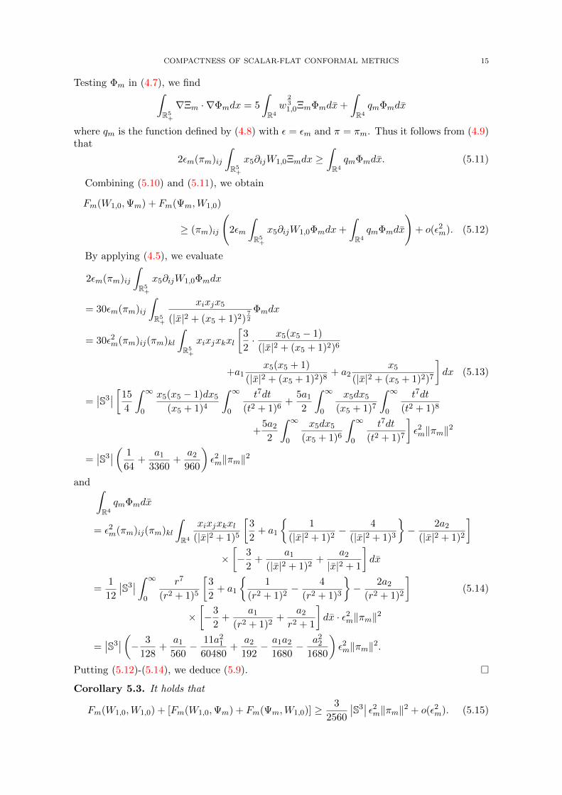
COMPACTNESS OF SCALAR-FLAT CONFORMAL METRICS 15
Testing Φm in (4.7), we find∫R5+
∇Ξm · ∇Φmdx = 5
∫R4
w231,0ΞmΦmdx+
∫R4
qmΦmdx
where qm is the function defined by (4.8) with ε = εm and π = πm. Thus it follows from (4.9)that
2εm(πm)ij
∫R5+
x5∂ijW1,0Ξmdx ≥∫R4
qmΦmdx. (5.11)
Combining (5.10) and (5.11), we obtain
Fm(W1,0,Ψm) + Fm(Ψm,W1,0)
≥ (πm)ij
(2εm
∫R5+
x5∂ijW1,0Φmdx+
∫R4
qmΦmdx
)+ o(ε2m). (5.12)
By applying (4.5), we evaluate
2εm(πm)ij
∫R5+
x5∂ijW1,0Φmdx
= 30εm(πm)ij
∫R5+
xixjx5
(|x|2 + (x5 + 1)2)72
Φmdx
= 30ε2m(πm)ij(πm)kl
∫R5+
xixjxkxl
[3
2· x5(x5 − 1)
(|x|2 + (x5 + 1)2)6
+a1x5(x5 + 1)
(|x|2 + (x5 + 1)2)8+ a2
x5
(|x|2 + (x5 + 1)2)7
]dx (5.13)
=∣∣S3∣∣ [15
4
∫ ∞0
x5(x5 − 1)dx5
(x5 + 1)4
∫ ∞0
t7dt
(t2 + 1)6+
5a1
2
∫ ∞0
x5dx5
(x5 + 1)7
∫ ∞0
t7dt
(t2 + 1)8
+5a2
2
∫ ∞0
x5dx5
(x5 + 1)6
∫ ∞0
t7dt
(t2 + 1)7
]ε2m‖πm‖2
=∣∣S3∣∣ ( 1
64+
a1
3360+
a2
960
)ε2m‖πm‖2
and ∫R4
qmΦmdx
= ε2m(πm)ij(πm)kl
∫R4
xixjxkxl(|x|2 + 1)5
[3
2+ a1
{1
(|x|2 + 1)2− 4
(|x|2 + 1)3
}− 2a2
(|x|2 + 1)2
]×[−3
2+
a1
(|x|2 + 1)2+
a2
|x|2 + 1
]dx
=1
12
∣∣S3∣∣ ∫ ∞
0
r7
(r2 + 1)5
[3
2+ a1
{1
(r2 + 1)2− 4
(r2 + 1)3
}− 2a2
(r2 + 1)2
](5.14)
×[−3
2+
a1
(r2 + 1)2+
a2
r2 + 1
]dx · ε2m‖πm‖2
=∣∣S3∣∣ (− 3
128+
a1
560− 11a2
1
60480+
a2
192− a1a2
1680− a2
2
1680
)ε2m‖πm‖2.
Putting (5.12)-(5.14), we deduce (5.9). �
Corollary 5.3. It holds that
Fm(W1,0,W1,0) + [Fm(W1,0,Ψm) + Fm(Ψm,W1,0)] ≥ 3
2560
∣∣S3∣∣ ε2m‖πm‖2 + o(ε2m). (5.15)

16 SEUNGHYEOK KIM, MONICA MUSSO, AND JUNCHENG WEI
Proof. From (5.8) and (5.9), we conclude that
Fm(W1,0,W1,0) + [Fm(W1,0,Ψm) + Fm(Ψm,W1,0)] ≥∣∣S3∣∣P (a1, a2)ε2m‖πm‖2 + o(ε2m)
where
P (a1, a2) = − 3
128+
a1
480− 11a2
1
60480+
a2
160− a1a2
1680− a2
2
1680.
It holds that
maxa1,a2∈R
P (a1, a2) = P
(−63
4,105
8
)=
3
2560.
Hence the assertion follows. �
Completion of the proof of Proposition 5.1 for N = 5. Owing to (5.2), (5.4), (5.5) and (5.15),it holds that
Cε3m ≥3
2560
∣∣S3∣∣ ε2m‖πm‖2 + o(ε2m).
Accordingly,
Cεm ≥3
2560
∣∣S3∣∣ ‖πm‖2 + o(1).
This implies that Proposition 5.1 holds for N = 5. �
Case N = 6: The strategy is the same as the cases N = 5. By inserting n = 5 and γ = 12 in
(5.9) of [32], one can compute that
Fm(W1,0,W1,0) = o(ε2m).
Also, computing as in Lemma 5.2, we obtain
Lemma 5.4. It holds that
Fm(W1,0,Ψm) + Fm(Ψm,W1,0)
≥∣∣S4∣∣ (− π
320+
a1π
3584− 3a2
1π
163840+
a2π
1280− a1a2π
16384− a2
2π
16384
)ε2m‖πm‖2 + o(ε2m).
Choosing the parameters a1 = −1287 and a2 = 544
35 , we get
Corollary 5.5. It holds that
Fm(W1,0,W1,0) + [Fm(W1,0,Ψm) + Fm(Ψm,W1,0)] ≥ 31π
78400
∣∣S3∣∣ ε2m‖πm‖2 + o(ε2m).
From this, the desired result (5.1) for N = 6 follows.
Case N = 4: Because of the integrability issue on W1,0, the computation becomes a littlebit trickier than before. Especially, it turns out that the terms involving a1 and a2 contributenothing. This is because the integrals involving them are O(ε2m), while the main order of
P1m(Vm, ρε−1m ) is ε2m log(ε−1
m ). Hence we set a1 = a2 = 0.
Lemma 5.6. It holds that
Fm(W1,0,W1,0) = − π
24
∣∣S2∣∣ ‖πm‖2ε2m log(ρε−1
m ) +O(ε2m). (5.16)
Proof. Lemma 2.2 and the Gauss-Codazzi equation implies that
R[gm](εmx) = −‖πm‖2 +O(εm|x|) in B5+(0, ρε−1
m ).
From this, Lemma 2.1 (more precisely, Lemmas 3.1 and 3.2 of [21]) and (5.7), we find that
Fm(W1,0,W1,0) = F0m + F1m + F2m +O(ε2m) (5.17)
where
F0m =1
6ε2m
∫B4
+(0,ρε−1m )
R[gm](εmx)W1,0Z01,0dx

COMPACTNESS OF SCALAR-FLAT CONFORMAL METRICS 17
= −1
6ε2m‖πm‖2
∫B4
+(0,ρε−1m )
W1,0Z01,0dx+O(ε2m),
F1m =
∫B4
+(0,ρε−1m )
(δij − gijm)∂ijW1,0Z1,0dx
= −1
3ε2m[3‖πm‖2 +RNN [gm](ym)
] ∫B4
+(0,ρε−1m )
x24∆xW1,0Z
01,0dx+O(ε2m)
= −2
3ε2m‖πm‖2
∫B4
+(0,ρε−1m )
x24∆xW1,0Z
01,0dx+O(ε2m)
and
F2m = −∫B4
+(0,ρε−1m )
(∂a√|gm|√|gm|
)gabm∂bW1,0Z1,0dx
= ε2m[‖πm‖2 +RNN [gm](ym)
] ∫B4
+(0,ρε−1m )
gabm∂bW1,0Z1,0dx+O(ε2m) = O(ε2m).
(5.18)
On the other hand, since∫B4
+(0,ρε−1m )
W1,0Z01,0dx
=
∫ ρε−1m
0
∫R3
1− |x|2 − x24
(|x|2 + (x4 + 1)2)3dxdx4 +O(1)
= −∣∣S2∣∣ [∫ ρε−1
m
0
dx4
x4 + 1
∫ ∞0
t4dt
(t2 + 1)3+
∫ ρε−1m
0
x24dx4
(x4 + 1)3
∫ ∞0
t2dt
(t2 + 1)3
]+O(1)
= −π4
∣∣S2∣∣ log(ρε−1
m ) +O(1),
we haveF0m =
π
24
∣∣S2∣∣ ‖πm‖2ε2m log(ρε−1
m ) +O(ε2m). (5.19)
Moreover, ∫B4
+(0,ρε−1m )
x24∆xW1,0Z
01,0dx
= 2
∫ ρε−1m
0
∫R3
x24
[|x|2 − 3(x4 + 1)2
](1− |x|2 − x2
4)
(|x|2 + (x4 + 1)2)5dx
= −2∣∣S2∣∣ ∫ ρε−1
m
0
∫ ∞0
r2x24
[r2 − 3(x4 + 1)2
](r2 + x2
4)
(r2 + (x4 + 1)2)5drdx4 +O(1)
=π
8
∣∣S2∣∣ log(ρε−1
m ) +O(1),
from which we deduce that
F1m = − π
12
∣∣S2∣∣ ‖πm‖2ε2m log(ρε−1
m ) +O(ε2m). (5.20)
Combining (5.17)-(5.20), we obtain (5.16). �
Unlike the cases N = 5 and 6, we do not exploit the mountain pass structure of theboundary Yamabe problem in RN+ . Instead, we use the integrability (or the decay property)of the functions involving the problem.
We define
Φδ(x) = επijxixj
[x4 − 1
(|x|2 + (x4 + 1)2)2+
δ
(|x|2 + (x4 + 1)2)32
](5.21)

18 SEUNGHYEOK KIM, MONICA MUSSO, AND JUNCHENG WEI
for δ small, which resembles the modified correction term ψε,δ defined in Page 400 of [42]. Ifδ = 0, the function Φδ is reduced to Φ in (4.5) with a1 = a2 = 0. Let also Ξδ = Ψ−Φδ whereΨ is the solution of (4.1). Then it satisfies
−∆Ξδ =9δεπijxixj
(|x|2 + (x4 + 1)2)52
in R4+,
− limx4→0
∂Ξδ∂x4
= 4w1,0Ξδ + qδ on R3
(5.22)
where
qδ(x) =επijxixj
(|x|2 + 1)2+
δεπijxixj
(|x|2 + 1)52
on R3.
Lemma 5.7. It holds that
εm [Fm(W1,0,Ψm) + Fm(Ψm,W1,0)]
≥(π
24+
64
105δ +O(δ2)
) ∣∣S2∣∣ ε2m log(ρε−1
m )‖πm‖2 +O(ε2m) (5.23)
for δ small.
Proof. Let Φm,δ be the function Φδ in (5.21) with ε = εm and π = πm. Set Ξm,δ and qm,δ inan analogous manner. By (4.5) and (4.2) of [32], it holds that
|Φm,δ(x)|+ |Ξm,δ(x)| ≤ Cεm|πm|∞1 + |x|
and |∇Φm,δ(x)|+ |∇Ξm,δ(x)| ≤ Cεm|πm|∞1 + |x|2
(5.24)
where |πm|∞ = maxi,j=1,2,3 |(πm)ij |. Integrating by parts, and employing (5.24),∫B3(0,ρε−1
m )
dx
1 + |x|3 + (ρε−1m )3
≤∣∣S2∣∣ ∫ ρε−1
m
0
r2dr
r3 + (ρε−1m )3
=∣∣S2∣∣ ∫ 1
0
dt
t3 + 1= O(1)
and ∫ ρε−1m
0
∫∂B3(0,ρε−1
m )
dx
1 + |x|3≤ C
∫ ρε−1m
0
(ρε−1m )2dx4
1 + (ρε−1m )3 + x3
4
≤ C∫ 1
0
dt
t3 + 1= O(1),
we calculate that
Fm(W1,0,Ψm) + Fm(Ψm,W1,0)
= −2εm(πm)ij
∫ ρε−1m
0
∫B3(0,ρε−1
m )x4 [∂ijW1,0 (xk∂kΨm + x4∂4Ψm + Ψm)
+∂ijΨm (xk∂kW1,0 + x4∂4W1,0 +W1,0)] dxdx4 +O(ε2m)
= 2εm(πm)ij
∫ ρε−1m
0
∫B3(0,ρε−1
m )x4 [4 ∂iW1,0∂jΨm + ∂iW1,0(xk∂jkΨm + x4∂j4Ψm) (5.25)
+(xk∂ikW1,0 + x4∂i4W1,0)∂jΨm] dx+O(ε2m)
= −2εm(πm)ij
∫ ρε−1m
0
∫B3(0,ρε−1
m )x4∂iW1,0∂jΨmdx+O(ε2m)
= 2εm(πm)ij
∫ ρε−1m
0
∫B3(0,ρε−1
m )(x4∂ijW1,0Φm,δ + x4∂ijW1,0Ξm,δ) dx+O(ε2m).
On the other hand, by testing Ξm,δ in (4.1) and applying (5.24) once more, we obtain
2εm(πm)ij
∫ ρε−1m
0
∫B3(0,ρε−1
m )x4∂ijW1,0Ξm,δdx
COMPACTNESS OF SCALAR-FLAT CONFORMAL METRICS 19
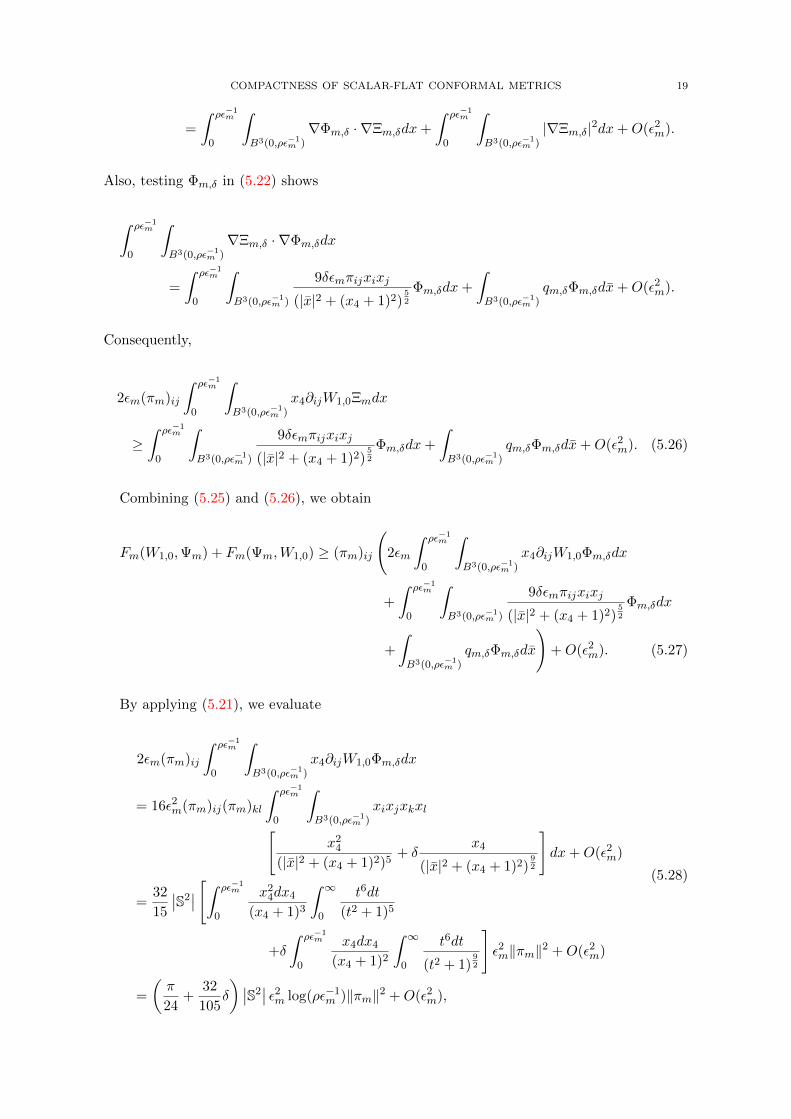
=
∫ ρε−1m
0
∫B3(0,ρε−1
m )∇Φm,δ · ∇Ξm,δdx+
∫ ρε−1m
0
∫B3(0,ρε−1
m )|∇Ξm,δ|2dx+O(ε2m).
Also, testing Φm,δ in (5.22) shows
∫ ρε−1m
0
∫B3(0,ρε−1
m )∇Ξm,δ · ∇Φm,δdx
=
∫ ρε−1m
0
∫B3(0,ρε−1
m )
9δεmπijxixj
(|x|2 + (x4 + 1)2)52
Φm,δdx+
∫B3(0,ρε−1
m )qm,δΦm,δdx+O(ε2m).
Consequently,
2εm(πm)ij
∫ ρε−1m
0
∫B3(0,ρε−1
m )x4∂ijW1,0Ξmdx
≥∫ ρε−1
m
0
∫B3(0,ρε−1
m )
9δεmπijxixj
(|x|2 + (x4 + 1)2)52
Φm,δdx+
∫B3(0,ρε−1
m )qm,δΦm,δdx+O(ε2m). (5.26)
Combining (5.25) and (5.26), we obtain
Fm(W1,0,Ψm) + Fm(Ψm,W1,0) ≥ (πm)ij
(2εm
∫ ρε−1m
0
∫B3(0,ρε−1
m )x4∂ijW1,0Φm,δdx
+
∫ ρε−1m
0
∫B3(0,ρε−1
m )
9δεmπijxixj
(|x|2 + (x4 + 1)2)52
Φm,δdx
+
∫B3(0,ρε−1
m )qm,δΦm,δdx
)+O(ε2m). (5.27)
By applying (5.21), we evaluate
2εm(πm)ij
∫ ρε−1m
0
∫B3(0,ρε−1
m )x4∂ijW1,0Φm,δdx
= 16ε2m(πm)ij(πm)kl
∫ ρε−1m
0
∫B3(0,ρε−1
m )xixjxkxl[
x24
(|x|2 + (x4 + 1)2)5+ δ
x4
(|x|2 + (x4 + 1)2)92
]dx+O(ε2m)
=32
15
∣∣S2∣∣ [∫ ρε−1
m
0
x24dx4
(x4 + 1)3
∫ ∞0
t6dt
(t2 + 1)5
+δ
∫ ρε−1m
0
x4dx4
(x4 + 1)2
∫ ∞0
t6dt
(t2 + 1)92
]ε2m‖πm‖2 +O(ε2m)
=
(π
24+
32
105δ
) ∣∣S2∣∣ ε2m log(ρε−1
m )‖πm‖2 +O(ε2m),
(5.28)

20 SEUNGHYEOK KIM, MONICA MUSSO, AND JUNCHENG WEI
9δεm(πm)ij
∫ ρε−1m
0
∫B3(0,ρε−1
m )
xixj
(|x|2 + (x4 + 1)2)52
Φm,δdx
= 9δε2m(πm)ij(πm)kl
∫ ρε−1m
0
∫B3(0,ρε−1
m )
xixjxkxlx4
(|x|2 + (x4 + 1)2)92
dx
+O(δ2 log(ρε−1m )‖πm‖2) +O(ε2m)
=6
35δ∣∣S2∣∣ ε2m log(ρε−1
m )‖πm‖2 +O(δ2 log(ρε−1m )‖πm‖2) +O(ε2m)
(5.29)
and ∫B3(0,ρε−1
m )qm,δΦm,δdx = ε2mδ(πm)ij(πm)kl
∫B3(0,ρε−1
m )
xixjxkxl
(|x|2 + 1)72
dx+O(ε2m)
=2
15δ∣∣S2∣∣ ε2m log(ρε−1
m )‖πm‖2.(5.30)
Putting (5.27)-(5.30), we deduce (5.23). �
Corollary 5.8. It holds that
Fm(W1,0,W1,0) + [Fm(W1,0,Ψm) + Fm(Ψm,W1,0)]
≥(
64
105δ +O(δ2)
) ∣∣S2∣∣ ε2m log(ρε−1
m )‖πm‖2 +O(ε2m)
for δ small.
Proof. The result immediately follows from (5.16) and (5.23). �
Completion of the proof of Proposition 5.1 for N = 4. By taking δ > 0 in Corollary 5.8 smallenough, we infer from (5.2), (5.4) and (5.5) that
Cε2m ≥32
105δ∣∣S2∣∣ ε2m log(ρε−1
m )‖πm‖2 +O(ε2m).
Accordingly,
C
| log εm|≥ ‖πm‖2 +O
(1
| log εm|
).
This implies that Proposition 5.1 holds for N = 4. �
6. Local sign restriction and set of blow-up points
Under the validity of Proposition 5.1, we derive the local sign restriction of the functionP.
Proposition 6.1. Assume that N ≥ 4 and ym → y0 ∈ ∂M is an isolated simple blow-uppoint for the sequence {Um}m∈N to the solutions to (2.5). Then, given m ∈ N large and ρ > 0small, there exist constants C0 ≥ 0 and C1, C2, C3 > 0 independent of m and ρ such that
εN−2+o(1)m P ′
(Um(0)Um, ρ
)≥ ε2mC0−ε2+η
m ρ2−ηC1−εN−2m ρ−N+3C2−
εN−1m ρN−1C3
ε2(N−1)+o(1)m + ρ2(N−1)+o(1)
for N ≥ 5 and
ε2+o(1)m P ′
(Um(0)Um, ρ
)≥ ε2m log(1 + ρε−1
m ) C0 − ε2mC1 −ε3mρ
3C2
ε6+o(1)m + ρ6+o(1)
for N = 4, in gm-Fermi coordinates centered in ym. Here, P ′ is the function defined in (2.7),
η > 0 is an arbitrarily small number and εo(1)m → 1 as m→∞.

COMPACTNESS OF SCALAR-FLAT CONFORMAL METRICS 21
Proof. If N ≥ 5, the proof follows the same lines as that of Lemma 6.1 in [32]; cf. Theorem7.2 of [2]. Slightly modifying the argument, one can also establish the inequality for N = 4.Here we allow the possibility that π[g0](y0) = 0 as opposed to [32]. Thus we cannot excludethat C1 = 0. �
From the previous proposition, we conclude the following results. It can be derived as inSection 6 of [32].
Lemma 6.2. Assume that N ≥ 4, and y0 ∈ ∂M is an isolated blow-up point for the sequence{Um}m∈N to (2.5). Then it is an isolated simple blow-up point of {Um}m∈N.
Proposition 6.3. Assume the hypotheses of Theorem 1.1. Let ε0, ε1, R, C0 and C1 be pos-itive numbers in the statement of Proposition 3.2. Suppose that U ∈ H1(M) is a solutionto (2.5) and {y1, · · · , yN } is the set of its local maxima on ∂M . Then there exists a con-stant C2 > 0 depending only on (M, g), N , ε0, ε1 and R such that if max∂M U ≥ C0, thendh(ym1 , ym2) ≥ C2 for all 1 ≤ m1 6= m2 ≤ N (U). In particular, the set of blow-up points of{Um}m∈N is finite and it consists of isolated simple blow-up points.
7. The compactness result
Using Proposition 5.1, namely, the assertion that π[g0](y0) = 0, we will verify the conditionsnecessary to apply the positive mass theorem (described in Lemma 2.4) for 4-manifolds. Notethat the number d in (2.10) is 1.
Lemma 7.1. Suppose that N = 4 or 5, y0 ∈ ∂M is an isolated simple blow-up point of thesequence {Um}m∈N of the solutions to (2.5). If we take κ ≥ 4 in (2.1), we can expand themetric g = g0 as in (2.10) and (2.11).
Proof. By Lemma 2.1 and Proposition 5.1, it clearly holds that
AiN (x) = ANN (x) = 0 and Aij(x) = O(|x|2).
Therefore,
expA(x) = I +A(x) +O(|x|4) and so g(x) = expA(x) +O(|x|4)
where I is the N ×N -identity matrix. From this, we see that
det g(x) = etraceA(x)+O(|x|4) = 1 + trace(A(x)) +O(|x|4).
By virtue of our choice κ ≥ 4, it follows that trace(A(x)) = O(|x|4) as desired. �
Lemma 7.2. Under the assumptions of Lemma 7.1, (2.12) holds for N = 4.
Proof. Setting κ ≥ 4 in Lemma 2.1 and applying Proposition 5.1, we obtain
SymklmRikjl,m[h] = SymklH,kl[g] = RNN,k[g] = RNN,N [g] = 0 at y0 (7.1)
where g = g0.By (2.11), (2.2), (7.1), the Ricci identity and the symmetry of the integral, the left-hand
side of (2.12) equals∫∂IB
N+ (0,ρ)
(ρ3−2Nxi∂jAij(x)− 2Nρ1−2NxixjAij(x)
)dSx
= ρ5−N |Sn−1|[
2(N − 3)
(N − 1)(N + 1)(N + 3)
]π[g]ij,ij(y0) +O(ρ6−N )
for any N ≥ 4. If N = 4, (2.12) immediately follows. �
22 SEUNGHYEOK KIM, MONICA MUSSO, AND JUNCHENG WEI
Lemma 7.3. Suppose that N = 4 or 5, and y0 ∈ ∂M is an isolated simple blow-up point ofthe sequence {Um}m∈N of the solutions to (2.5). Let Gy0 be the normalized Green’s functionof the conformal Laplacian with Neumann boundary condition with pole at y0, that is, thesolution of (2.17). If we choose the integer κ in (2.1) large enough, it holds that
Gy0(x) =
{|x|−2 +O(| log |x||) if N = 4,
|x|−3 +O(|x|−1| log |x||) if N = 5
in g0-Fermi coordinates centered at y0. As a particular consequence, Gy0 is a smooth positivefunction on M \ {y0} which can be expressed as (2.13)-(2.14).
Proof. We will employ Proposition B.2 of [6], in which Almaraz and Sun constructed theGreen’s function on manifolds with boundary using parametrices.
According to their result, if there exists a sufficiently large integer κ0 such that
|H[g0](y)| ≤ Cdg0(y, y0)κ0 for all y ∈ ∂M, (7.2)
then one can find a smooth positive solution Gy0 on M \{y0} to (2.17) with g = g0. Moreover,if g0 = expB for some 2-tensor B on M , then
∣∣Gy0(x)− |x|2−N∣∣ ≤ C n∑
i,j=1
d∑|α|=1
|Bij,α(0)| |x||α|+2−N +
{C|x|d+3−N for N ≥ 5,
C(1 + | log |x||) for N = 3, 4
(7.3)in g0-Fermi coordinates centered at y0, where d = bN−2
2 c as before. Check also (1.3) for thenotations involving multi-indices.
Differentiating (3.4) of [21] |β|-times, we obtain
∂
∂xN
∂√|g0|
∂xβ(x, 0) = −n
∑β′+β′′=β
β!
β′!β′′!
∂√|h0|
∂xβ′
∂H[g0]
∂xβ′′
(x) for x ∈ Rn, (7.4)
in normal coordinates on ∂M centered at y0. Here h0 is the restriction of g0 to ∂M . In lightof (2.1) and (7.4), the coefficient of xβxN in the Taylor expansion of
√|g0| at x = 0 has to
be
− n
(|β|+ 1)!
∂βH[g0]
∂xβ(0) = 0 for all |β| ≤ κ− 1.
Thus, if we take κ ≥ κ0, all partial derivatives of H of order ≤ κ0 − 1 must vanish at 0, andso (7.2) holds.
On the other hand, we know that A(x) = O(|x|2) and g0 = expA+O(|x|4) from the proofof Lemma 7.1. Therefore, for |α| = 1,
Bij,α(x) = Aij,α(x) +O(|x|) = O(|x|), and so Bij,α(0) = 0.
This implies that the right-hand side of (7.3) is bounded by{C|x|4−N = C|x|−1 = O(|x|−1| log |x||) for N = 5,
C(|x|4−N + 1 + | log |x||) = C(1 + | log |x||) = O(| log |x||) for N = 4.
The proof is finished. �
We are now ready to complete the proof of our main result.
Proof of Theorem 1.1. Suppose that y0 ∈ ∂M is a blow-up point of of the sequence {Um}m∈Nof the solutions to (2.5). By Proposition 6.3, it is isolated simple. By Proposition 3.5 andelliptic regularity theory, there also exists a function G = Gy0 and a constant a > 0 such that
Um(ym)Um → aG in C2(Bg0(y0, ρ) \ {y0}) as m→∞

COMPACTNESS OF SCALAR-FLAT CONFORMAL METRICS 23
and (2.17) holds. Thanks to Proposition 6.1, it follows that
lim infρ→0
P ′(aG, ρ) = a2 lim infρ→0
P ′(G, ρ) ≥ 0. (7.5)
Assume that N = 4. Because of Lemmas 7.1-7.3, all the conditions necessary to applyLemma 2.4 hold. Besides, (2.17) implies (2.16). In view of (2.15),
lim infρ→0
P ′(G, ρ) < 0,
contradicting (7.5). Consequently, there is no blow-up point of a solution to (2.5), whichmeans that its solution set is L∞(M)-bounded. Elliptic regularity tells us that it is C2(M)-compact. Hence Theorem 1.1 must be valid in this case.
We next assume that N = 5 or 6 and the trace-free second fundamental form π[g] nevervanishes on ∂M . There is a positive smooth function ω0 on M such that g0 = ω0g on M .In Proposition 1.2 of [22], it was proved that π[g0] =
√ω π[g] on ∂M . We now reach a
contradiction, since Proposition 5.1 leads
0 = ‖π[g0](y0)‖ = ω(y0)−12 ‖π[g](y0)‖ > 0.
This concludes the proof of Theorem 1.1. �
Remark 7.4. Note that Lemmas 7.1 and 7.3 work for N = 5. Therefore, if we couldshow that the tensor π[g0]ij,ij(y0) in the proof of Lemma 7.2 vanishes2, we would be able toapply the positive mass theorem and deduce Theorem 1.1 for all 5-manifolds not conformallyequivalent to B5.
Considering the energy expansion, one can say that the boundary Yamabe problem for 4-or 5-manifolds corresponds to the classical Yamabe problem for 6- or 7-manifolds, respec-tively. In this case, the corresponding quantity to π[g0]ij,ij is, say, a sum Rij,ij(0) of thesecond derivatives of the scalar curvature at 0. In the proof of Theorem 7.3 of [40], Marquesdiscovered that
Rij,ij(0) = −1
2R,jj(0) = −1
2∆R(0) =
1
12‖W (0)‖2 = 0
where W is the Weyl tensor and the last equality comes from the Weyl vanishing theorem(Theorem 6.1 of [40]). From this observation, he could establish the C2-compactness resultnot only for 6-dimensional manifolds but for 7-dimensional ones as well.
Appendix A. Proof of Lemmas 4.3 and 4.5
Throughout this section, we assume that N ≥ 5. The case N = 4 can be handled similarly.
In order to prove Lemma 4.3, we first need two preliminary observations.
Lemma A.1. Suppose that N ≥ 5. The function
Φ1(x) =1
4(N − 4)
xN + 1
(|x|2 + (xN + 1)2)N−4
2
+ a1xN + 1
(|x|2 + (xN + 1)2)N2
in RN+
for a1 ∈ R satisfies
−∆Φ1 =xN + 1
(|x|2 + (xN + 1)2)N−2
2
in RN+ .
Proof. It holds that
xN + 1
(|x|2 + (xN + 1)2)N−2
2
= −(
1
N − 4
)∂N
[1
(|x|2 + (xN + 1)2)N−4
2
]in RN+ .
2The Codazzi equation, the contracted second Bianchi identity and (7.1) show that π[g0]ij,ij(y0) =−RiN,i[g0](y0) = − 1
2R,N [g0](y0).
24 SEUNGHYEOK KIM, MONICA MUSSO, AND JUNCHENG WEI
Thus, if we have a solution Φ0 of the equation
−∆Φ0 =1
(|x|2 + (xN + 1)2)N−4
2
in RN+ ,
we will be able to choose
Φ1 = −(
1
N − 4
)∂NΦ0. (A.1)
On the other hand, we see that
−∆[Φ0(x, xN − 1)] =1
(|x|2 + x2N )
N−42
=1
|x|N−4in Rn × (1,∞).
If we assume that Φ0(x, xN − 1) is radial symmetric, i.e., φ0(|x|) = Φ0(x, xN − 1), then it isreduced to
−φ′′0 −N − 1
rφ′0 =
1
rN−4in (0,∞).
Its general solution is expressed as
φ0(r) =
1
4(N − 6)
1
rN−6+
a1
rN−2+ a′1 if N = 5 or N ≥ 7,
− log r
4+a1
r4+ a′1 if N = 6
for r ∈ (0,∞) and a1, a′1 ∈ R. Consequently,
Φ0(x) =
1
4(N − 6)
1
(|x|2 + (xN + 1)2)N−6
2
+a1
(|x|2 + (xN + 1)2)N−2
2
+ a2
if N = 5 or N ≥ 7,
−1
8log(|x|2 + (xN + 1)2) +
a1
(|x|2 + (xN + 1)2)2+ a′1
if N = 6
(A.2)
in RN+ .By (A.1) and (A.2), the assertion in the statement holds. �
Lemma A.2. The function
Φ2(x) =1
2(N − 4)
1
(|x|2 + (xN + 1)2)N−4
2
+ a21
(|x|2 + (xN + 1)2)N−2
2
+ a′2 in RN+
for a2, a′2 ∈ R satisfies
−∆Φ2 =1
(|x|2 + (xN + 1)2)N−2
2
in RN+ . (A.3)
Proof. Equation (A.3) is equivalent to
−∆[Φ2(x, xN − 1)] =1
(|x|2 + x2N )
N−22
=1
|x|N−2in RN+ .
If we assume that Φ2(x, xN − 1) is radial symmetric, i.e., φ2(|x|) = Φ2(x, xN − 1), then it isreduced to
−φ′′2 −n
rφ′2 =
1
rN−2in (0,∞).
The general solution is expressed as
φ2(r) =1
2(N − 4)rN−4+
a2
rN−2+ a′2
for r ∈ (0,∞) and a2, a′2 ∈ R. As a result, the assertion in the statement holds. �
COMPACTNESS OF SCALAR-FLAT CONFORMAL METRICS 25
Corollary A.3. The function
(Φ1 − Φ2)(x) =1
4(N − 4)
xN − 1
(|x|2 + (xN + 1)2)N−4
2
+ a1xN + 1
(|x|2 + (xN + 1)2)N2
+ a21
(|x|2 + (xN + 1)2)N−2
2
+ a′2
in RN+
for a1, a2, a′2 ∈ R satisfies
−∆(Φ1 − Φ2) =xN
(|x|2 + (xN + 1)2)N−2
2
= xNW1,0 in RN+ .
Proof. It is a direct consequence of Lemmas A.1 and A.2. �
Completion of the proof of Lemma 4.3. Define Φij = ∂ij(Φ1 − Φ2) so that Φ = 2πijΦij . ByCorollary A.3,
Φij(x) = −xN − 1
4
[δij
(|x|2 + (xN + 1)2)N−2
2
− (N − 2)xixj
(|x|2 + (xN + 1)2)N2
]
+ a1(xN + 1)
[δij
(|x|2 + (xN + 1)2)N+2
2
− (N + 2)xixj
(|x|2 + (xN + 1)2)N+4
2
]
+ a2
[δij
(|x|2 + (xN + 1)2)N2
−N xixj
(|x|2 + (xN + 1)2)N+2
2
] in RN+ .
Since the trace of π is assumed to be 0, we have (4.5). This completes the proof. �
Completion of the proof of Lemma 4.5. It follows from (4.1) and (4.6) that U is harmonic inRN+ . Note also that
limxN→0
∂U
∂xN+Nw
2N−2
1,0 U = − limxN→0
∂Φ
∂xN−Nw
2N−2
1,0 Φ on Rn.
Plugging (4.5) into the right-hand side, we find the boundary condition that U satisfies. �
Acknowledgement. S. Kim is supported by Basic Science Research Program throughthe National Research Foundation of Korea(NRF) funded by the Ministry of Education(NRF2017R1C1B5076384), and the associate member problem of Korea institute for ad-vanced study(KIAS). M. Musso has been supported by Fondecyt grant 1160135. The researchof J. Wei is partially supported by NSERC of Canada.
References
[1] S. Almaraz, An existence theorem of conformal scalar-flat metrics on manifolds with boundary, PacificJ. Math. 248 (2010), 1–22.
[2] , A compactness theorem for scalar-flat metrics on manifolds with boundary, Calc. Var. PartialDifferential Equations 41 (2011), 341–386.
[3] , Blow-up phenomena for scalar-flat metrics on manifolds with boundary, J. Differential Equations251 (2011), 1813–1840.
[4] S. Almaraz, E. Barbosa, L. L. de Lima, A positive mass theorem for asymptotically flat manifoldswith a non-compact boundary, Comm. Anal. Geom. 24 (2016), 673–715.
[5] S. Almaraz, O. S. de Queiroz, S. Wang, A compactness theorem for scalar-flat metrics on 3-manifoldswith boundary, J. Funct. Anal. in press.
[6] S. Almaraz, L. Sun, Convergence of the Yamabe flow on manifolds with minimal boundary, Ann. Sc.Norm. Super. Pisa Cl. Sci., in press.
[7] T. Aubin, Equations differentielles non lineaires et probleme de Yamabe concernant la courbure scalaire,J. Math. Pures Appl. 55 (1976), 269–296.
[8] S. Brendle, Blow-up phenomena for the Yamabe equation, J. Amer. Math. Soc. 21 (2008), 951–979.[9] S. Brendle, F. Marques, Blow-up phenomena for the Yamabe equation II, J. Differential Geom. 81
(2009), 225–250.

26 SEUNGHYEOK KIM, MONICA MUSSO, AND JUNCHENG WEI
[10] E. Cardenas, W. Sierra, Uniqueness of solutions of the Yamabe problem on manifolds with boundary,Nonlinear Anal. 187 (2019), 125–133.
[11] S. S. Chen, Conformal deformation to scalar at metrics with constant mean curvature on the boundaryin higher dimensions, preprint, arXiv:0912.1302.
[12] P. Cherrier, Problemes de Neumann non lineaires sur les varietes Riemannienes, J. Funct. Anal. 57(1984) 154–206.
[13] J. Davila, M. del Pino, Y. Sire, Nondegeneracy of the bubble in the critical case for nonlocal equations,Proc. Amer. Math. Soc. 141 (2013), 3865–3870.
[14] S. Deng, S. Kim, A. Pistoia, Linear perturbations of the fractional Yamabe problem on the minimalconformal infinity, to appear in Comm. Anal. Geom.
[15] M. M. Disconzi, M. A. Khuri, Compactness and non-compactness for the Yamabe problem on manifoldswith boundary, J. Reine Angew. Math. 724 (2017), 145–201.
[16] Z. Djadli, A. Malchiodi, M. Ould Ahmedou, Prescribing scalar and boundary mean curvature onthe three dimensional half sphere. J. Geom. Anal. 13 (2003), 255-289.
[17] , The prescribed boundary mean curvature problem on B4. J. Differential Equations 206 (2004),373–398.
[18] O. Druet, Compactness for Yamabe metrics in low dimensions, Int. Math. Res. Not. 23 (2004), 1143–1191.
[19] J. F. Escobar, Sharp constant in a Sobolev trace inequality, Indiana Univ. Math. J. 37 (1988), 687–698.[20] , Uniqueness theorems on conformal deformation of metrics, Sobolev inequalities, and an eigenvalue
estimate, Comm. Pure Appl. Math. 43 (1990), 857–883.[21] , Conformal deformation of a Riemannian metric to a scalar flat metric with constant mean
curvature on the boundary, Ann. of Math. 136 (1992), 1–50.[22] , The Yamabe problem on manifolds with boundary, J. Differential Geom. 35 (1992), 21–84.[23] , Conformal metrics with prescribed mean curvature on the boundary, Calc. Var. Partial Differ-
ential Equations 4 (1996), 559–592.[24] V. Felli, A. Ould Ahmedou, Compactness results in conformal deformations of Riemannian metrics
on manifolds with boundaries, Math. Z. 244 (2003), 175–210.[25] , A geometric equation with critical nonlinearity on the boundary, Pacific J. Math. 218 (2005),
75–99.[26] M. Ghimenti, A. M. Micheletti, A compactness result for scalar-flat metrics on manifolds with umbilic
boundary, preprint, arXiv:1903.10990.[27] M. Ghimenti, A. M. Micheletti, A. Pistoia Linear perturbation of the Yamabe problem on manifolds
with boundary, J. Geom. Anal. 28 (2018), 1315–1340.[28] , Blow-up phenomena for linearly perturbed Yamabe problem on manifolds with umbilic boundary,
J. Differential Equations 267 (2019), 587–618.[29] Z.-C. Han, Y. Y. Li, The Yamabe problem on manifolds with boundary: existence and compactness
results, Duke Math. J. 99 (1999), 485–542.[30] M. Khuri, F. Marques, R. Schoen, A compactness theorem for the Yamabe problem, J. Differential
Geom. 81 (2009), 143–196.[31] S. Kim, M. Musso, and J. Wei, Existence theorems of the fractional Yamabe problem, Anal. PDE 11
(2018), 75–113.[32] , A compactness theorem of the fractional Yamabe problem, Part I: The non-umbilic conformal
infinity. preprint, arXiv:1808.04951.[33] M. Mayer, C. B. Ndiaye, Barycenter technique and the Riemann mapping problem of Cherrier-Escobar,
J. Differential Geom. 107 (2017), 519–560.[34] G. Li, A compactness theorem on Branson’s Q-curvature equation, preprint, arXiv:1505.07692.[35] Y. Y. Li, J. Xiong, Compactness of conformal metrics with constant Q-curvature. I, Adv. Math. 345
(2019), 116–160.[36] Y. Y. Li, L. Zhang, Compactness of solutions to the Yamabe problem II, Calc. Var. and Partial Differ-
ential Equations 25 (2005), 185–237.[37] , Compactness of solutions to the Yamabe problem III, J. Funct. Anal. 245 (2006), 438–474.[38] Y. Li, M. Zhu, Uniqueness theorems through the method of moving spheres, Duke Math. J. 80 (1995),
383–417.[39] , Yamabe type equations on three dimensional Riemannian manifolds, Comm. Contemp. Math. 1
(1999), 1–50.[40] F. C. Marques, A priori estimates for the Yamabe problem in the non-locally conformally flat case, J.
Differential Geom. 71 (2005), 315–346.[41] , Existence results for the Yamabe problem on manifolds with boundary, Indiana Univ. Math. J.
54 (2005), 1599–1620.

COMPACTNESS OF SCALAR-FLAT CONFORMAL METRICS 27
[42] , Conformal deformations to scalar-flat metris with constant mean curvature on the boundary,Comm. Anal. Geom. 15 (2007), 381–405.
[43] R. Schoen, Course notes on ‘Topics in differential geometry’ at Stanford University, (1988), available athttps://www.math.washington.edu/~pollack/research/Schoen-1988-notes.html
(Seunghyeok Kim) Department of Mathematics and Research Institute for Natural Sciences,College of Natural Sciences, Hanyang University, 222 Wangsimni-ro Seongdong-gu, Seoul04763, Republic of Korea
Email address: [email protected] [email protected]
(Monica Musso) Department of Mathematical Sciences, University of Bath, Bath BA2 7AY,United Kingdom, and Facultad de Matematicas, Pontificia Universidad Catolica de Chile,Avenida Vicuna Mackenna 4860, Santiago, Chile
Email address: [email protected]
(Juncheng Wei) Department of Mathematics, University of British Columbia, Vancouver, B.C.,Canada, V6T 1Z2
Email address: [email protected]