Introduction - Mathjjohnson/research_files/gcms.pdf · Introduction Gas chromatography-mass ... A...
22
DECONVOLUTION IN GC/MS-LIKE SITUATIONS DREW JOHNSON 1. Introduction Gas chromatography-mass spectrometry (GC/MS) is a powerful method for iden- tifying chemical substances in complex mixtures. The use of this method introduces some interesting mathematical problems. A mass spectrometer works by fragment- ing a compound into ions. An ion detector can then count the intensity of ions with distinct mass to charge ratios, giving a mass spectrum. This mass spectrum is a fingerprint that can be matched against a library of known compounds. Mass spectrometry is useful for identifying uncontaminated, pure samples. A gas chro- matograph forces a sample through a column. Depending on the properties of the column, different compounds are retained in the column for different amounts of time. The amount of elution at the end of the column can be detected and recorded. Gas chromatographs are useful for separating compounds, but the retention time of a compound alone is not always enough to uniquely identify it. We can com- bine these techniques into a powerful “hyphenated method” by running the mass spectrometer multiple times as the sample elutes (comes out) from the column. However, especially when a mixture contains several similar compounds or when the sample is run through the column quickly, the elution times of some compounds may overlap. In this case, we may hope to deconvolve them by mathematical means. 2. Set up We have a M × T data matrix X, where M is the number of distinct mass to charge ratios that the scanner is set to detect, and T is the number of scans or observations. Each column of X is a linear combination of an unknown number, n, of unknown spectra of the actual components s 1 ,s 2 ,...s n . (In this paper, the word “spectra” is referring to mass spectra, a chemistry concept, rather than the mathematical concept with the same name.) Each pure component has an (also unknown) concentration profile (or elution profile), c 1 ,c 2 ,...,c n , which is a vector of length T that represents how much of the component eluted at any time. In other words, if c i are the rows of C and s i are the columns of S, X = SC Each entry of all three of these matrices is positive. Our goal is to recover the vectors s i . In general, factoring a matrix into two matrices this way is non-unique. By using additional assumptions or regularization criteria, we can attempt to identify good solutions. In the methods we tried, we assumed that the number of components n was known or could be estimated accurately. 1
Transcript of Introduction - Mathjjohnson/research_files/gcms.pdf · Introduction Gas chromatography-mass ... A...
DECONVOLUTION IN GC/MS-LIKE SITUATIONS
DREW JOHNSON
1. Introduction
Gas chromatography-mass spectrometry (GC/MS) is a powerful method for iden-tifying chemical substances in complex mixtures. The use of this method introducessome interesting mathematical problems. A mass spectrometer works by fragment-ing a compound into ions. An ion detector can then count the intensity of ionswith distinct mass to charge ratios, giving a mass spectrum. This mass spectrumis a fingerprint that can be matched against a library of known compounds. Massspectrometry is useful for identifying uncontaminated, pure samples. A gas chro-matograph forces a sample through a column. Depending on the properties of thecolumn, different compounds are retained in the column for different amounts oftime. The amount of elution at the end of the column can be detected and recorded.Gas chromatographs are useful for separating compounds, but the retention timeof a compound alone is not always enough to uniquely identify it. We can com-bine these techniques into a powerful “hyphenated method” by running the massspectrometer multiple times as the sample elutes (comes out) from the column.However, especially when a mixture contains several similar compounds or whenthe sample is run through the column quickly, the elution times of some compoundsmay overlap. In this case, we may hope to deconvolve them by mathematical means.
2. Set up
We have a M × T data matrix X, where M is the number of distinct mass tocharge ratios that the scanner is set to detect, and T is the number of scans orobservations. Each column of X is a linear combination of an unknown number,n, of unknown spectra of the actual components s1, s2, . . . sn. (In this paper, theword “spectra” is referring to mass spectra, a chemistry concept, rather than themathematical concept with the same name.) Each pure component has an (alsounknown) concentration profile (or elution profile), c1, c2, . . . , cn, which is a vectorof length T that represents how much of the component eluted at any time. Inother words, if ci are the rows of C and si are the columns of S,
X = SC
Each entry of all three of these matrices is positive. Our goal is to recover thevectors si.
In general, factoring a matrix into two matrices this way is non-unique. By usingadditional assumptions or regularization criteria, we can attempt to identify goodsolutions. In the methods we tried, we assumed that the number of components nwas known or could be estimated accurately.
1
2 DREW JOHNSON
3. Directly Fitting
One approach is to attempt to directly fit a model to the situation. We assumethat the elution profiles have shapes Cit = fθi
(t), where f is a family of functionswith parameters θ. Then, we must solve the optimization problem
min{θk},S
∣∣∣∣∣∣X − SC({θk})∣∣∣∣∣∣
where C({θk}) is the estimate for C using the parameters {θk}. If we use theFrobenius norm (and square the objective), this problem is linear in S. However,it may be quite non-linear in {θk}.
One model I have used for fθ is the family A exp(−(t−µσ
)2)with parameters A,
µ, and σ. This seems to be a reasonable approximation of shapes for concentrationprofiles.
The Nelder-Mead simplex method [4] was used to solve the optimization problem.The linearity in S makes this problem tractable; however, it seems to have manylocal minima, so a good starting point is critical. The most effective method wefound was to get a starting point for θ using an estimate for C from another methodsuch as NNMF or AR (discussed in Section 5). Several variations of this “DirectFit” algorithm were tested in Section 8. There is a two parameter method where thecoefficient A was omitted, and the family exp
(−(t−µσ
)2)was used for the fit, even
the the randomly generated examples used A exp(−(t−µσ
)2). In some situations,
this variation seems to perform better. We hypothesize that this is the case becausewhen these coefficients A were similar or the same, the algorithm would benefit byhaving fewer variables to optimize over and not be hurt too much by the loss offlexibility when fitting.
4. Using convexity
4.1. Normalizing. One very interesting way to approach this problem is to exploita normalization trick that turns the linear combinations into convex combinations.This trick was suggested by Grande and Manne in [1].
Let xt be the tth column of X. Take a unit vector p, with the properties thatxTt p > 0 for all xt, and p has no negative entries.
Now, we normalize by assigning
yt =xtpTxt
Geometrically, this amounts to truncating or extending each vector so that it liesin the hyperplane supported by p.
Now, that means the normalized spectra of the pure components are
ei =sipT si
.
DECONVOLUTION IN GC/MS-LIKE SITUATIONS 3
Now any xt, the tth column of X, is a linear combination of the pure spectraxt =
∑Citsi. Thus
yt =xtpTxt
(1)
=∑i
CitsipTxt
(2)
=∑i
CitsipTxt
pT sipT si
(3)
=∑i
sipT si
(Citp
T sipTxt
)(4)
=∑i
eiCitp
T sipTxt
.(5)
Now,∑i Citp
T si = pTxt, so∑iCitp
T si
pT xt= 1. Since Citp
T si
pT xt≥ 0 for all i, we have
that yt is a convex combination of e1, e2, . . . en.
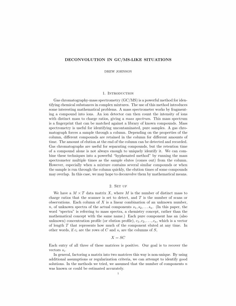
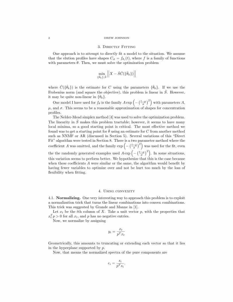
4.2. Finding S. Now, if each observation is a convex combination of a finite setof points, then each observation lies in a convex polytope with the pure spectra asvertices. Since X is of rank n (ignoring noise), and the normalization eliminatedone degree of freedom, we can represent these as points in n− 1 dimensional space,and now our polytope is a simplex. Figure 1 shows a graphical representation ofa hypothetical data matrix of a sample with three components with each ion (rowof X) plotted in a different color. Figure 2 shows a representation of these samedata (with loss of information about total intensity) as convex combinations of thevertices of a simplex (a triangle in this case).
We can examine the normalized observations yi, and then estimate where thevertices of the containing simplex lie. This problem is of course quite ill posed,since there are infinitely many simplices that contain a given set of points.
Looking at Figure 2, we may be tempted to choose the two “endpoints” as twoof our estimates for actual spectra, and then do two linear extrapolations using thefirst few points on each side, and calculating their intersection. This is the methodtested in Section 8 as “Convex Extrapolate”. However, for more difficult problemswhere the peaks are closely overlapping, the shape is not as “nice” as that seen in2, and the intersection of the extrapolations can be inside the convex hull of thedata, or in other unreasonable places. In addition, there is no sound theoreticaljustification for this method; it just seems natural geometrically.
We can make some improvements if we have some knowledge about the shapeof C. Since rows of C are “continuously” changing with respect to time, it seemsnatural to use a model similar to that used in Bezier curves. This kind of modeluses a partition of unity, which is a set of functions {mi(t)} where
∑imi(t) = 1.
The curve B is then defined by a set of control points, Pi, by
B(t) =∑i
miPi.
A standard nth degree polynomial Bezier curve uses the partition of unity definedby the Bernstein polynomials {bni (t) =
(ni
)ti(1 − t)n−i}. The algorithm “Convex,
Bezier Fit” (see Section 8 works by fitting a curve of this form to the data, and then
4 DREW JOHNSON
Figure 1. A plot of a hypothetical data matrix X.
Figure 2. A convex representation of Figure 1.
using the control points (transformed back into the original space) as estimates forthe actual spectra. This tends to produce better estimates than the extrapolationmethod. We can do better, however, if we use more assumptions about the shapesof the concentration profiles.
DECONVOLUTION IN GC/MS-LIKE SITUATIONS 5
In general, if we assume as in Section 3 that the components have shapes Cit =fΘi(t), it seems reasonable to use the partition of unity{
fθk(t)∑n
j=1 fθj (t)
}nk=1
.
This means that again we must solve an optimization problem involving minimizinga residual between the data and the fit, over the variables {θk} and the controlpoints. This is still a fairly complex problem with local minima. Although therepresentation of the data as a set of convex combinations is appealing, it is not yetcompletely clear what advantage this has over more direct methods like those inSection 3. However, empirical evidence suggests that it does perform well in certainsituations.
4.3. The Choice of p. The properties noted in Section 4.1 (p ≥ 0 and not orthog-onal to any xi) are sufficient to give the convexity property. The original paper[1] suggested using the first singular vector (the first column of U from the SVD).This seems reasonable because the span of the first n columns of the SVD is a goodestimate for the span of si.
One property that seems like it would be desirable would be to choose a p sothat pT si is the same for all i. This will give (from equation (5))
yt =pT s1
pTxt
∑i
fΘi(t)ei
=pT s1
pT∑i fΘi(t)si
∑i
fΘi(t)ei
=pT s1∑
i fΘi(t)pT si
∑i
fΘi(t)ei
=1
n∑i fΘi
(t)
∑i
fΘi(t)ei.
This is exactly the partition of unity (within a constant factor) that we suggested inSection 4.2. Thus, choosing this p ensures that, assuming the actual profiles reallydo come from the family fθ, our partition of unity model is accurate. A geometricway to describe this situation is that the simplex and its containing points aredetermined, within an affine transformation, only by C and not by S.
Vectors with the property that pT si is constant are not unique. Any will do,as long as pT si 6= 0. To avoid this and encourage numerical stability, we want tochoose p so that pT s1 is at a maximum. To find this p, if we assume we know si, wecan find the subspace P = {p : ST p = k1} which is equal to span{N (ST ) ∪ {p0}},where p0 is a particular solution to ST p = 1. Then, the best solution is s1 projectedonto this subspace, and normalized.
Numerical experiments suggest that this method is slightly better than the firstsingular vector method in some cases. However, testing this scheme requires us to“cheat” by using the actual values of si to calculate p. It is not clear whether thereis a good way to estimate this p, especially since the whole problem in the firstplace is to estimate si. We can use an estimate obtained by another method, suchas non-negative matrix factorization, as an estimate for si, and use this estimateto find p. This is the approach used in the “special” variations in Section 8.
6 DREW JOHNSON
Another option is to take the vector that supports the n-dimensional hyperplanethat passes through each of the si and normalize it. This seems to be geometricallysatisfying. Numerical experiments again suggest improvement over the first singularvector method, but we have the same problem of needing to know si in order tocalculate p.
In random tests the vectors p selected by both of these methods are quite sim-ilar to the first singular vector, especially when all the concentration profiles areapproximately the same size and shape.
All of these methods involve finding the intersections of rays with an affine space.Although the first alternative method preserves the ratios of the intensities of thecompounds, there is still some distortion, as two pairs of vectors with the sameangle between them will have different Euclidean distances between them in thespace where the simplex lives — the pair of vectors which are almost normal tothe plane may be closer than the pair which is less close to normal. This may be aproblem because when our optimization routine measures error, the error may bemeasured inconsistently. This issue could be resolved if we project the points ontothe unit sphere. This will still preserve convexity, and would cause none of thiskind of distortion, and also preserve the relative values of coefficients. However, itseems that it may complicate the computations in curve fitting and destroy whatlinearity we have.
In Section 8 these algorithms are referred to as “ConEx”, an acronym for “Nor-malization to produce Convexity followed by Exponential Fit”, with each combi-nation of the “special” and 2 and 3 parameter variations included.
5. Non-negative matrix factorization
The problem of factoring a positive matrix into a product of two positive ma-trices has applications in other areas as well, and several methods have been pro-posed. These methods are sometimes effective for the type of deconvolution we areattempting.
5.1. Alternating Regression. The method described in Algorithm 1 was sug-gested specifically for the type of deconvolution we are discussing [2].
Algorithm 1 Alternating Regression [2]
Require: Data matrix XFill S′ with random positive entries.repeatS ← S′
Calculate a least squares fit for C in X = SC: C ← (STS)−1STX.Set the negative entries of C to zero.Force C to be unimodal by setting secondary humps to zero.Calculate a least squares fit for S′ in X = S′C: S′ = (CCT )−1CXT .Set the negative entries of S′ to zero.
until ||S − S′|| < tol, where we use the Frobenius norm
The idea of this algorithm is to produce a factorization that “looks good” basedon some assumptions about the shape of the concentration profiles. The assump-tions suggested by [2] are non-negativity and unimodality. This method may seem
DECONVOLUTION IN GC/MS-LIKE SITUATIONS 7
ad hoc, but it works surprisingly well in many situations. Notice that the algorithmis non-deterministic, as it uses a random starting point, so one variation is to runthe algorithm several times with different starting points. However, as the algo-rithm always produces outputs that “look good” it may be tricky to choose whichoutput is the desirable one.
5.2. Other non-negative matrix factorizations (NNMF). More well knownnon-negative matrix factorizations include a multiplicative update method, such asthat described by Lee and Seung [3]. Traditional alternating least squares methodsalso exist. They differ from Algorithm 1 in that they solve the least squares problemwith a positivity constraint, and omit the coercion towards unimodality. MATLABprovides two implementations of NNMF — a multiplicative one, and an alternatingleast squares. We empirically found the alternating least squares implementationto be more effective for our application.
6. Peak Maximization Methods
In real applications in GC/MS, the spectra of actual compounds are usuallysparse in the sense that they have many zero entries. This introduces the possibilityof using methods which attempt to find ions which are unique to each component.This is the basic premise of AMDIS, one of the standards in the industry. Themethod of AMDIS is described in a paper by Stein [5]. Here, we describe a simplemethod which uses essentially the same ideas.
First, the MATLAB curve fitting toolbox function fit is run on each row ofthe data, using the smoothingspline option. Other types of fitting may also beappropriate, but the important point is to have a polynomial model (or anothertype of model that can be evaluated quickly) so we can interpolate between thedata and simulate a higher resolution. We find the times of local maxima in themodel and record them. We then use a clustering algorithm to group them inton groups. We then take the median of each group, and any ions that maximize“close” to it, and add them up and use that for an estimate of the concentrationprofile. We then do a non-negative least squares fit to these profiles to estimateS. This method seems to work quite well in practice when the data is sparse. Ofcourse it fails completely in the non-sparse case.
Two variations of this idea are seen in Sections 8. They differ in the setting ofparameters. The first is the increase in resolution when evaluating the fit, and thesecond is a parameter that controls how close an ions maximization has to be tothe median in order for it to be considered as part of the estimation of the profileshape.
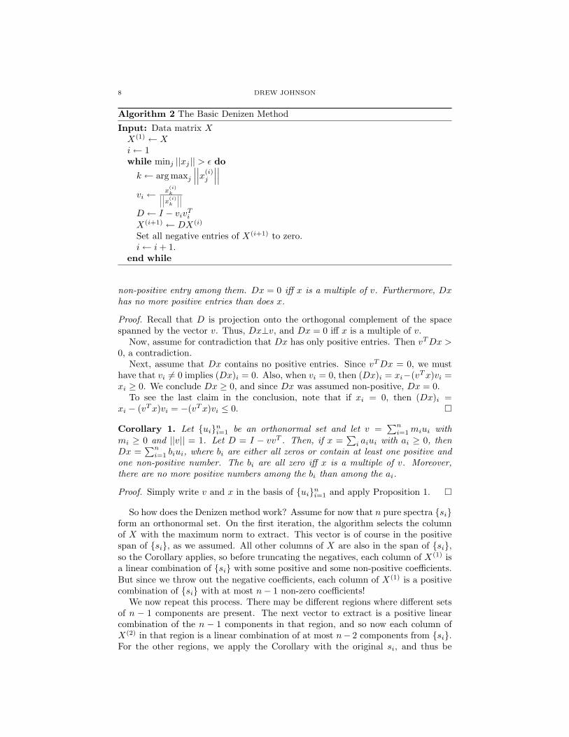
7. The Denizen Method
The Denizen method was developed by James Oliphant and others at Torion.The author has done some analysis to explain why it works.
The first round of the “Denizen” algorithm is given in Algorithm 2. We hopethat spectra of the original components will be among the extracted vectors vi.
The following observations will help us justify the use of this algorithm.
Proposition 1. Let v, x ≥ 0 (entry-wise), with ||v|| = 1. Let D = I − vvT . Then,either Dx = 0, or the entries of the vector Dx have at least one positive and one
8 DREW JOHNSON
Algorithm 2 The Basic Denizen MethodInput: Data matrix XX(1) ← Xi← 1while minj ||xj || > ε do
k ← arg maxj∣∣∣∣∣∣x(i)
j
∣∣∣∣∣∣vi ←
x(i)k∣∣∣∣∣∣x(i)k
∣∣∣∣∣∣D ← I − vivTiX(i+1) ← DX(i)
Set all negative entries of X(i+1) to zero.i← i+ 1.
end while
non-positive entry among them. Dx = 0 iff x is a multiple of v. Furthermore, Dxhas no more positive entries than does x.
Proof. Recall that D is projection onto the orthogonal complement of the spacespanned by the vector v. Thus, Dx⊥v, and Dx = 0 iff x is a multiple of v.
Now, assume for contradiction that Dx has only positive entries. Then vTDx >0, a contradiction.
Next, assume that Dx contains no positive entries. Since vTDx = 0, we musthave that vi 6= 0 implies (Dx)i = 0. Also, when vi = 0, then (Dx)i = xi−(vTx)vi =xi ≥ 0. We conclude Dx ≥ 0, and since Dx was assumed non-positive, Dx = 0.
To see the last claim in the conclusion, note that if xi = 0, then (Dx)i =xi − (vTx)vi = −(vTx)vi ≤ 0. �
Corollary 1. Let {ui}ni=1 be an orthonormal set and let v =∑ni=1miui with
mi ≥ 0 and ||v|| = 1. Let D = I − vvT . Then, if x =∑i aiui with ai ≥ 0, then
Dx =∑ni=1 biui, where bi are either all zeros or contain at least one positive and
one non-positive number. The bi are all zero iff x is a multiple of v. Moreover,there are no more positive numbers among the bi than among the ai.
Proof. Simply write v and x in the basis of {ui}ni=1 and apply Proposition 1. �
So how does the Denizen method work? Assume for now that n pure spectra {si}form an orthonormal set. On the first iteration, the algorithm selects the columnof X with the maximum norm to extract. This vector is of course in the positivespan of {si}, as we assumed. All other columns of X are also in the span of {si},so the Corollary applies, so before truncating the negatives, each column of X(1) isa linear combination of {si} with some positive and some non-positive coefficients.But since we throw out the negative coefficients, each column of X(1) is a positivecombination of {si} with at most n− 1 non-zero coefficients!
We now repeat this process. There may be different regions where different setsof n − 1 components are present. The next vector to extract is a positive linearcombination of the n − 1 components in that region, and so now each column ofX(2) in that region is a linear combination of at most n− 2 components from {si}.For the other regions, we apply the Corollary with the original si, and thus be
DECONVOLUTION IN GC/MS-LIKE SITUATIONS 9
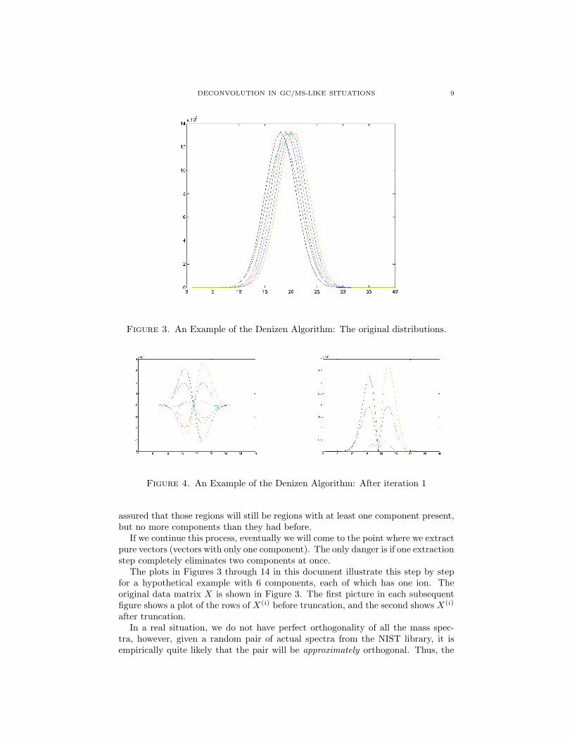
Figure 3. An Example of the Denizen Algorithm: The original distributions.
Figure 4. An Example of the Denizen Algorithm: After iteration 1
assured that those regions will still be regions with at least one component present,but no more components than they had before.
If we continue this process, eventually we will come to the point where we extractpure vectors (vectors with only one component). The only danger is if one extractionstep completely eliminates two components at once.
The plots in Figures 3 through 14 in this document illustrate this step by stepfor a hypothetical example with 6 components, each of which has one ion. Theoriginal data matrix X is shown in Figure 3. The first picture in each subsequentfigure shows a plot of the rows of X(i) before truncation, and the second shows X(i)
after truncation.In a real situation, we do not have perfect orthogonality of all the mass spec-
tra, however, given a random pair of actual spectra from the NIST library, it isempirically quite likely that the pair will be approximately orthogonal. Thus, the
10 DREW JOHNSON
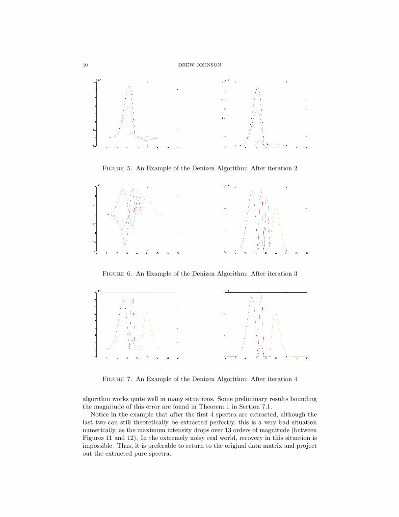
Figure 5. An Example of the Denizen Algorithm: After iteration 2
Figure 6. An Example of the Denizen Algorithm: After iteration 3
Figure 7. An Example of the Denizen Algorithm: After iteration 4
algorithm works quite well in many situations. Some preliminary results boundingthe magnitude of this error are found in Theorem 1 in Section 7.1.
Notice in the example that after the first 4 spectra are extracted, although thelast two can still theoretically be extracted perfectly, this is a very bad situationnumerically, as the maximum intensity drops over 13 orders of magnitude (betweenFigures 11 and 12). In the extremely noisy real world, recovery in this situation isimpossible. Thus, it is preferable to return to the original data matrix and projectout the extracted pure spectra.
DECONVOLUTION IN GC/MS-LIKE SITUATIONS 11
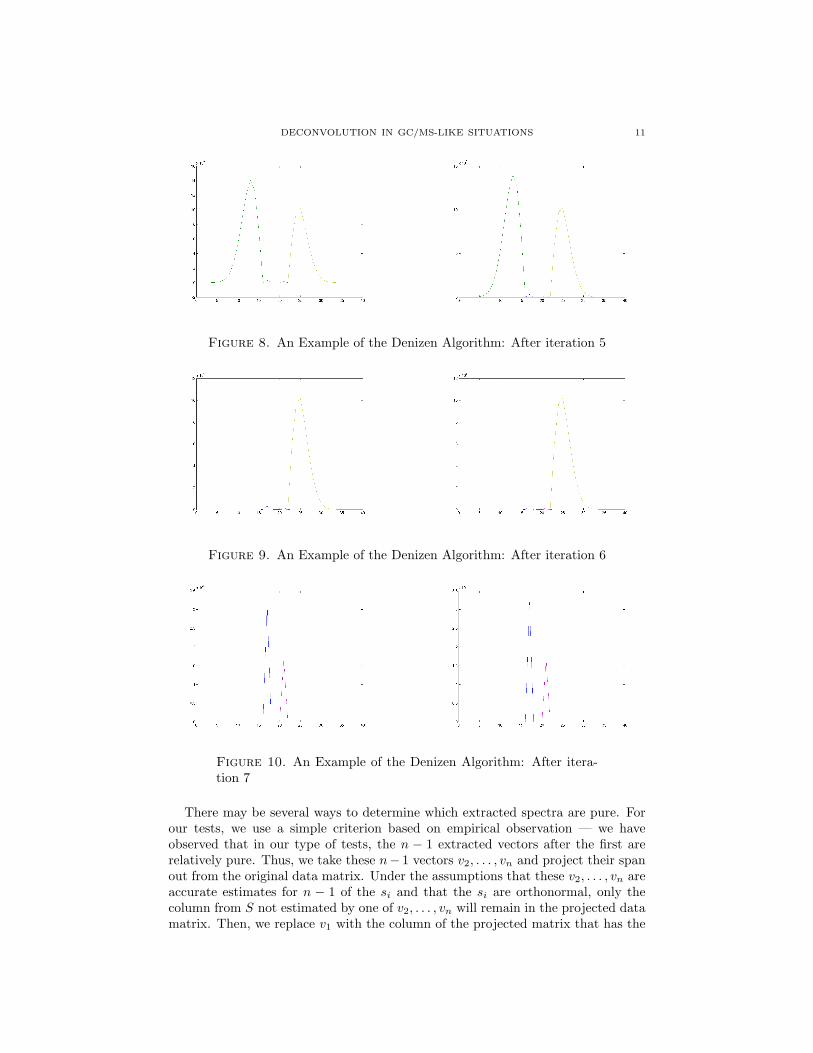
Figure 8. An Example of the Denizen Algorithm: After iteration 5
Figure 9. An Example of the Denizen Algorithm: After iteration 6
Figure 10. An Example of the Denizen Algorithm: After itera-tion 7
There may be several ways to determine which extracted spectra are pure. Forour tests, we use a simple criterion based on empirical observation — we haveobserved that in our type of tests, the n − 1 extracted vectors after the first arerelatively pure. Thus, we take these n− 1 vectors v2, . . . , vn and project their spanout from the original data matrix. Under the assumptions that these v2, . . . , vn areaccurate estimates for n − 1 of the si and that the si are orthonormal, only thecolumn from S not estimated by one of v2, . . . , vn will remain in the projected datamatrix. Then, we replace v1 with the column of the projected matrix that has the
12 DREW JOHNSON
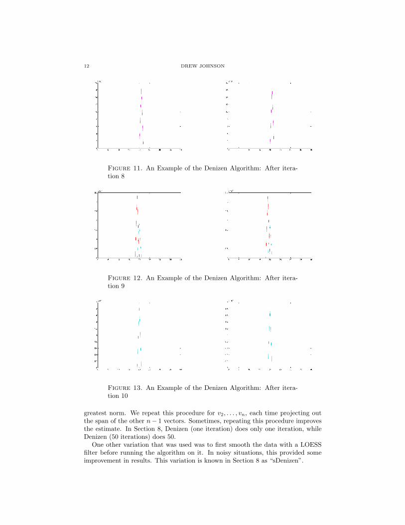
Figure 11. An Example of the Denizen Algorithm: After itera-tion 8
Figure 12. An Example of the Denizen Algorithm: After itera-tion 9
Figure 13. An Example of the Denizen Algorithm: After itera-tion 10
greatest norm. We repeat this procedure for v2, . . . , vn, each time projecting outthe span of the other n− 1 vectors. Sometimes, repeating this procedure improvesthe estimate. In Section 8, Denizen (one iteration) does only one iteration, whileDenizen (50 iterations) does 50.
One other variation that was used was to first smooth the data with a LOESSfilter before running the algorithm on it. In noisy situations, this provided someimprovement in results. This variation is known in Section 8 as “sDenizen”.
DECONVOLUTION IN GC/MS-LIKE SITUATIONS 13
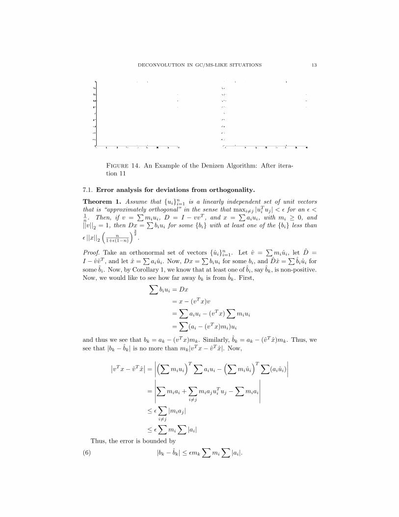
Figure 14. An Example of the Denizen Algorithm: After itera-tion 11
7.1. Error analysis for deviations from orthogonality.
Theorem 1. Assume that {ui}ni=1 is a linearly independent set of unit vectorsthat is “approximately orthogonal” in the sense that maxi6=j |uTi uj | < ε for an ε <1n . Then, if v =
∑miui, D = I − vvT , and x =
∑aiui, with mi ≥ 0, and
||v||2 = 1, then Dx =∑biui for some {bi} with at least one of the {bi} less than
ε ||x||2(
n1+ε(1−n)
) 32.
Proof. Take an orthonormal set of vectors {ui}ni=1. Let v =∑miui, let D =
I − vvT , and let x =∑aiui. Now, Dx =
∑biui for some bi, and Dx =
∑biui for
some bi. Now, by Corollary 1, we know that at least one of bi, say bk, is non-positive.Now, we would like to see how far away bk is from bk. First,∑
biui = Dx
= x− (vTx)v
=∑
aiui − (vTx)∑
miui
=∑
(ai − (vTx)mi)ui
and thus we see that bk = ak − (vTx)mk. Similarly, bk = ak − (vT x)mk. Thus, wesee that |bk − bk| is no more than mk|vTx− vT x|. Now,
∣∣vTx− vT x∣∣ =∣∣∣∣(∑miui
)T∑aiui −
(∑miui
)T∑(aiui)
∣∣∣∣=
∣∣∣∣∣∣∑
miai +∑i6=j
miajuTi uj −
∑miai
∣∣∣∣∣∣≤ ε
∑i6=j
|miaj |
≤ ε∑
mi
∑|ai|
Thus, the error is bounded by
(6) |bk − bk| ≤ εmk
∑mi
∑|ai|.
14 DREW JOHNSON
Next, we need bounds on∑|ai| and
∑mi. We can get such bounds by solving
the following maximization problem:
max{ai},{ui}
∑ai(7)
s.t. ||x||22 = k
|uTi uj | < ε
The symbol k is an arbitrary parameter. First, we notice that ||x||22 =∑a2i +∑
i6=j aiajuTi uj . Next, we claim that the {ai} are positive at the optimal point. If
one were negative, say ak, making it positive would increase the the value of theobjective function. Of course, this may violate the constraint, but if we simplychange uk to −uk the constraint is again satisfied. Now, we change the equalityconstraint to an inequality constraint. We will see that this does not change theoptimal value of the objective. Now, knowing that {ai} are positive, and that thechoice of {ui} affects only the constraint, we choose ui so that uTi uj = −ε for all iand j in order to make the constraint as loose as possible. We also transform theproblem into a minimization problem. Thus, our problem becomes
min{ai}
−∑
ai
s.t.∑
a2i − ε
∑i 6=j
aiaj − k ≤ 0
Now the objective function is linear, and the inequality constraint is convex for ε ≤1n . This is verified in Lemma 1. Thus, a point which satisfies the KKT conditionsis in in fact an optimal point. The stationarity conditions for this problem are
∂
∂akΛ({ai}, µ) = −1 + µ(2ak − 2ε
∑i6=k
ai) = 0
Solving for µ gives
µ =1
2ak − 2ε∑i 6=k ai
Since this is true for all k, the symmetry inherent in this set of equations impliesthat ak = aj for all k, j. We also see that by complementary slackness, since µ 6= 0,we know the constraint is active as we claimed. We denote the value of ai by a?,and then plugging into the original constraint, we get
na?2 − εa?2(n2 − n)− k = 0
whence
a? = ±√k
√n√
1 + ε(1− n).
In order to maintain dual feasibility, we choose the positive value for a?. The valueof the objective function for the original problem (7) at a? is∑
a? =
√nk√
1 + ε(1− n).
DECONVOLUTION IN GC/MS-LIKE SITUATIONS 15
Applying this to our particular problem, we have∑|ai| ≤
√n ||x||2√
1 + ε(1− n)∑mi ≤
√n√
1 + ε(1− n)
mi ≤√n√
1 + ε(1− n)
Thus, from (6) we see that the error is bounded by
|bk − bk| ≤ ε ||x||2
(n
1 + ε(1− n)
) 32
.
�
Lemma 1. The function∑ni=1 a
2i − ε
∑i 6=j aiaj is convex for 0 ≤ ε < 1
n .
Proof. The Hessian is a matrix with 2 in every entry on the diagonal and −2ε ineach other entry:
2 −2ε . . . −2ε
−2ε. . . . . .
......
. . . . . . −2ε−2ε . . . −2ε 2
If we can show that the Hessian is positive definite, then we will have shown thatthe function is convex. Equivalently, we consider the matrix
H(n) =
1 −ε . . . −ε
−ε. . . . . .
......
. . . . . . −ε−ε . . . −ε 1
We use Sylvester’s criteria for determining if a matrix is positive definite: if them ×m submatrix in the top left corner has a positive determinant for every 1 ≤m ≤ n, then the matrix is positive definite.
First, we claim that the r × r matrix
M(r) =
1 −ε . . . −ε −ε
−ε. . . . . .
......
.... . . . . . −ε
...
−ε . . . −ε 1...
−ε . . . . . . . . . −ε
has determinant −ε(1+ε)r−1. Applying cofactor expansion along the top row we seethat except for the first and last entry of the top row, each submatrix correspondingto an entry of the top row has two columns equal to −ε1, so these have determinant
16 DREW JOHNSON
0. Thus,
detM(r) = detM(r − 1)− (−1)r+1ε
−ε 1 −ε . . . −ε... −ε
. . . . . ....
......
. . . . . . −ε... −ε . . . −ε 1−ε . . . . . . . . . −ε
where the matrix shown is r − 1 × r − 1. Note that this matrix has determinant(−1)r−2 detM(r−1), as it can be transformed into M(r−1) by r−2 transpositionsof columns. Thus, we get the recurrence relation
detM(r) = detM(r − 1)− (−1)2r−1εdetM(r − 1)
= detM(r − 1)(1 + ε).
The formula follows from this recurrence relation and the initial condition detM(1) =−ε.
Now, we consider the determinant of H(n). Again applying cofactor expansionalong the top row, note that the submatrix corresponding to the first entry isH(n − 1). The submatrix corresponding to the second entry can be transformedinto M(n− 1) by 2(n− 2) transpositions— move the first column to the end, andthe first row to the bottom. Thus, this submatrix has the same determinant asM(n − 1). Now, the submatrix corresponding to the third entry of the first rowcan be transformed into the the submatrix corresponding to the second by onetransposition of rows. Using similar arguments we find the recurrence relation
detH(n) = detH(n− 1) +n∑i=2
(−ε)(−1)i−1(−1)i detM(n− 1)
= detH(n− 1)− (n− 1)ε2(1 + ε)n−1
Now, we argue by induction, using this relationship and with initial conditiondetH(2) = 1− ε2, that
detH(n) = (1− n)(1 + ε)n−1(ε− 1n− 1
).
for n ≥ 2. Assume the formula holds for n− 1. Then, by the recurrence relation
detH(n) = (2− n)(1 + ε)n−2(ε− 1n− 2
)− (n− 1)ε2(1 + ε)n−1
= (1 + ε)n−2
((2− n)(ε− 1
n− 2) + (1− n)ε2
)= (1 + ε)n−2
((2− n)ε+ 1 + (1− n)ε2
)= (1 + ε)n−2(ε+ 1)((1− n)ε+ 1)
= (1− n)(1 + ε)n−1
(ε− 1
n− 1
)We thus see that H(n) is positive on
(−1, 1
n−1
), which proves the lemma. �
The Denizen algorithm assumes that after the first projection and truncation,any column of X(2) is a linear combination of at most n−1 of the actual components
DECONVOLUTION IN GC/MS-LIKE SITUATIONS 17
si. If the orthogonality assumptions are not satisfied, then this may not be true.However, Theorem 1 assures us that any column of X(2) is a linear combination of
n− 1 of the actual components contaminated by no more than ε ||x||2(
n1+ε(1−n)
) 32
of another unit vector. For example in a three component system with ε = .01, thisamounts to 5.36% of ||xt||.
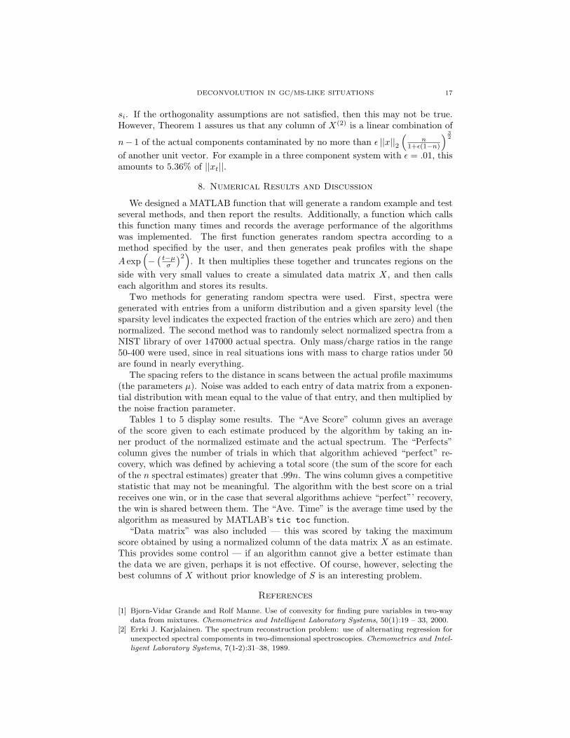
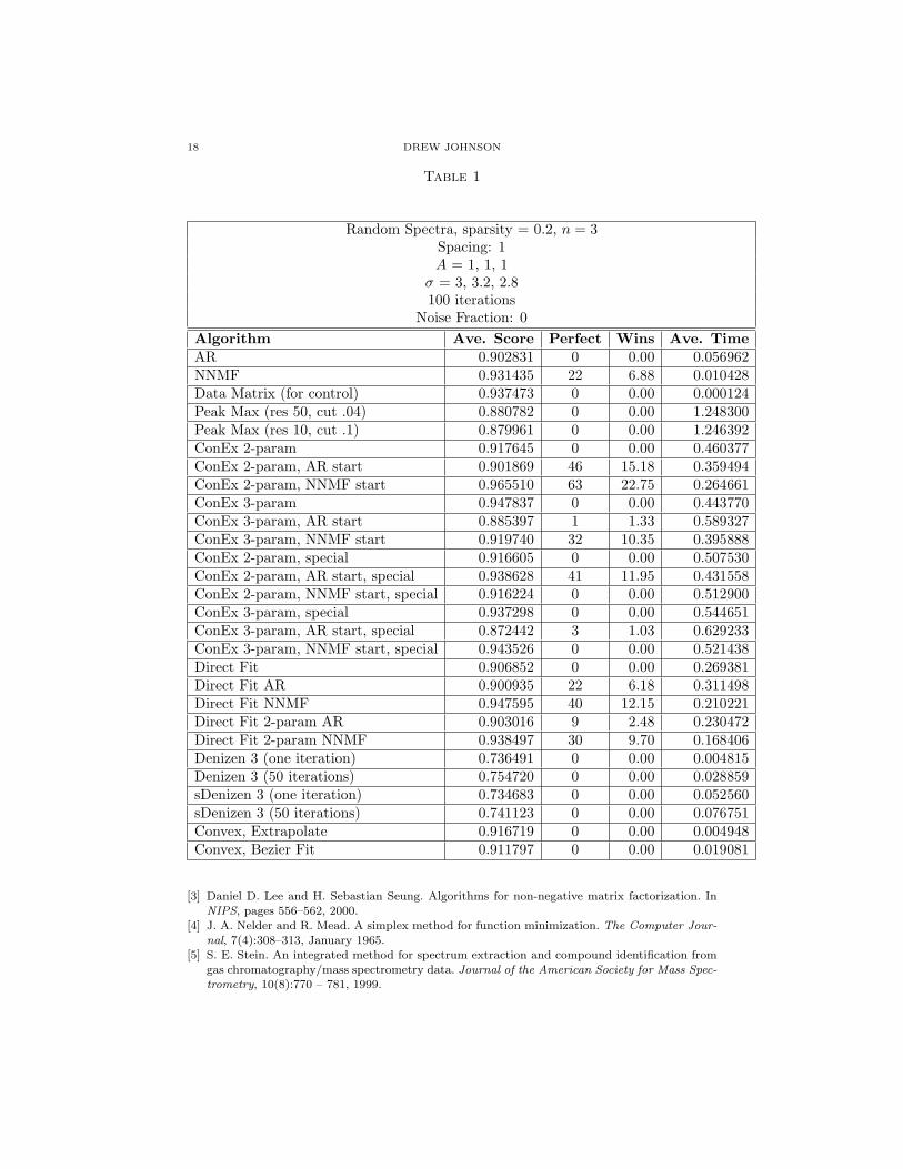
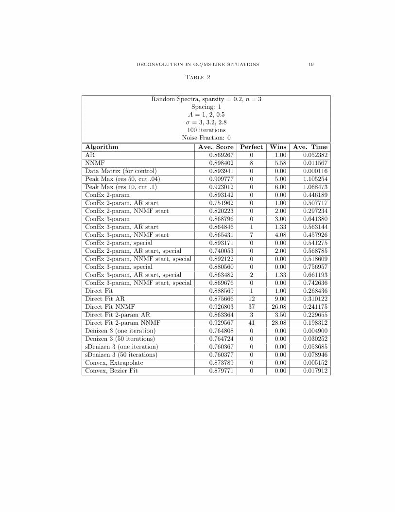
8. Numerical Results and Discussion
We designed a MATLAB function that will generate a random example and testseveral methods, and then report the results. Additionally, a function which callsthis function many times and records the average performance of the algorithmswas implemented. The first function generates random spectra according to amethod specified by the user, and then generates peak profiles with the shapeA exp
(−(t−µσ
)2). It then multiplies these together and truncates regions on the
side with very small values to create a simulated data matrix X, and then callseach algorithm and stores its results.
Two methods for generating random spectra were used. First, spectra weregenerated with entries from a uniform distribution and a given sparsity level (thesparsity level indicates the expected fraction of the entries which are zero) and thennormalized. The second method was to randomly select normalized spectra from aNIST library of over 147000 actual spectra. Only mass/charge ratios in the range50-400 were used, since in real situations ions with mass to charge ratios under 50are found in nearly everything.
The spacing refers to the distance in scans between the actual profile maximums(the parameters µ). Noise was added to each entry of data matrix from a exponen-tial distribution with mean equal to the value of that entry, and then multiplied bythe noise fraction parameter.
Tables 1 to 5 display some results. The “Ave Score” column gives an averageof the score given to each estimate produced by the algorithm by taking an in-ner product of the normalized estimate and the actual spectrum. The “Perfects”column gives the number of trials in which that algorithm achieved “perfect” re-covery, which was defined by achieving a total score (the sum of the score for eachof the n spectral estimates) greater that .99n. The wins column gives a competitivestatistic that may not be meaningful. The algorithm with the best score on a trialreceives one win, or in the case that several algorithms achieve “perfect”’ recovery,the win is shared between them. The “Ave. Time” is the average time used by thealgorithm as measured by MATLAB’s tic toc function.
“Data matrix” was also included — this was scored by taking the maximumscore obtained by using a normalized column of the data matrix X as an estimate.This provides some control — if an algorithm cannot give a better estimate thanthe data we are given, perhaps it is not effective. Of course, however, selecting thebest columns of X without prior knowledge of S is an interesting problem.
References
[1] Bjorn-Vidar Grande and Rolf Manne. Use of convexity for finding pure variables in two-waydata from mixtures. Chemometrics and Intelligent Laboratory Systems, 50(1):19 – 33, 2000.
[2] Errki J. Karjalainen. The spectrum reconstruction problem: use of alternating regression for
unexpected spectral compoments in two-dimensional spectroscopies. Chemometrics and Intel-ligent Laboratory Systems, 7(1-2):31–38, 1989.
18 DREW JOHNSON
Table 1
Random Spectra, sparsity = 0.2, n = 3Spacing: 1A = 1, 1, 1
σ = 3, 3.2, 2.8100 iterations
Noise Fraction: 0Algorithm Ave. Score Perfect Wins Ave. TimeAR 0.902831 0 0.00 0.056962NNMF 0.931435 22 6.88 0.010428Data Matrix (for control) 0.937473 0 0.00 0.000124Peak Max (res 50, cut .04) 0.880782 0 0.00 1.248300Peak Max (res 10, cut .1) 0.879961 0 0.00 1.246392ConEx 2-param 0.917645 0 0.00 0.460377ConEx 2-param, AR start 0.901869 46 15.18 0.359494ConEx 2-param, NNMF start 0.965510 63 22.75 0.264661ConEx 3-param 0.947837 0 0.00 0.443770ConEx 3-param, AR start 0.885397 1 1.33 0.589327ConEx 3-param, NNMF start 0.919740 32 10.35 0.395888ConEx 2-param, special 0.916605 0 0.00 0.507530ConEx 2-param, AR start, special 0.938628 41 11.95 0.431558ConEx 2-param, NNMF start, special 0.916224 0 0.00 0.512900ConEx 3-param, special 0.937298 0 0.00 0.544651ConEx 3-param, AR start, special 0.872442 3 1.03 0.629233ConEx 3-param, NNMF start, special 0.943526 0 0.00 0.521438Direct Fit 0.906852 0 0.00 0.269381Direct Fit AR 0.900935 22 6.18 0.311498Direct Fit NNMF 0.947595 40 12.15 0.210221Direct Fit 2-param AR 0.903016 9 2.48 0.230472Direct Fit 2-param NNMF 0.938497 30 9.70 0.168406Denizen 3 (one iteration) 0.736491 0 0.00 0.004815Denizen 3 (50 iterations) 0.754720 0 0.00 0.028859sDenizen 3 (one iteration) 0.734683 0 0.00 0.052560sDenizen 3 (50 iterations) 0.741123 0 0.00 0.076751Convex, Extrapolate 0.916719 0 0.00 0.004948Convex, Bezier Fit 0.911797 0 0.00 0.019081
[3] Daniel D. Lee and H. Sebastian Seung. Algorithms for non-negative matrix factorization. InNIPS, pages 556–562, 2000.
[4] J. A. Nelder and R. Mead. A simplex method for function minimization. The Computer Jour-
nal, 7(4):308–313, January 1965.
[5] S. E. Stein. An integrated method for spectrum extraction and compound identification fromgas chromatography/mass spectrometry data. Journal of the American Society for Mass Spec-
trometry, 10(8):770 – 781, 1999.
DECONVOLUTION IN GC/MS-LIKE SITUATIONS 19
Table 2
Random Spectra, sparsity = 0.2, n = 3Spacing: 1A = 1, 2, 0.5σ = 3, 3.2, 2.8100 iterations
Noise Fraction: 0Algorithm Ave. Score Perfect Wins Ave. TimeAR 0.869267 0 1.00 0.052382NNMF 0.898402 8 5.58 0.011567Data Matrix (for control) 0.893941 0 0.00 0.000116Peak Max (res 50, cut .04) 0.909777 0 5.00 1.105254Peak Max (res 10, cut .1) 0.923012 0 6.00 1.068473ConEx 2-param 0.893142 0 0.00 0.446189ConEx 2-param, AR start 0.751962 0 1.00 0.507717ConEx 2-param, NNMF start 0.820223 0 2.00 0.297234ConEx 3-param 0.868796 0 3.00 0.641380ConEx 3-param, AR start 0.864846 1 1.33 0.563144ConEx 3-param, NNMF start 0.865431 7 4.08 0.457926ConEx 2-param, special 0.893171 0 0.00 0.541275ConEx 2-param, AR start, special 0.740053 0 2.00 0.568785ConEx 2-param, NNMF start, special 0.892122 0 0.00 0.518609ConEx 3-param, special 0.880560 0 0.00 0.756957ConEx 3-param, AR start, special 0.863482 2 1.33 0.661193ConEx 3-param, NNMF start, special 0.869676 0 0.00 0.742636Direct Fit 0.888569 1 1.00 0.268436Direct Fit AR 0.875666 12 9.00 0.310122Direct Fit NNMF 0.926803 37 26.08 0.241175Direct Fit 2-param AR 0.863364 3 3.50 0.229655Direct Fit 2-param NNMF 0.929567 41 28.08 0.198312Denizen 3 (one iteration) 0.764808 0 0.00 0.004900Denizen 3 (50 iterations) 0.764724 0 0.00 0.030252sDenizen 3 (one iteration) 0.760367 0 0.00 0.053685sDenizen 3 (50 iterations) 0.760377 0 0.00 0.078946Convex, Extrapolate 0.873789 0 0.00 0.005152Convex, Bezier Fit 0.879771 0 0.00 0.017912
20 DREW JOHNSON
Table 3
Randomly selected spectra from NIST library, n = 3Spacing: 1
A = 1, 1.2, 0.8σ = 3, 3.2, 2.8
100 trialsNoise Fraction: 0
Algorithm Ave. Score Perfect Wins Ave. TimeAR 0.802218 0 0.00 0.040509NNMF 0.811569 2 0.61 0.016489Data Matrix (for control) 0.835624 0 0.00 0.000161Peak Max (res 50, cut .04) 0.978118 82 22.00 2.213887Peak Max (res 10, cut .1) 0.995378 89 24.45 2.161557ConEx 2-param 0.787877 0 0.00 0.525585ConEx 2-param, AR start 0.740140 0 0.00 0.405827ConEx 2-param, NNMF start 0.786760 1 1.25 0.347952ConEx 3-param 0.829842 0 0.00 0.558452ConEx 3-param, AR start 0.760581 0 0.00 0.672346ConEx 3-param, NNMF start 0.851573 6 2.14 0.386555ConEx 2-param, special 0.789884 0 0.00 0.572529ConEx 2-param, AR start, special 0.750165 2 0.50 0.539195ConEx 2-param, NNMF start, special 0.789854 0 0.00 0.560172ConEx 3-param, special 0.832925 0 0.00 0.655680ConEx 3-param, AR start, special 0.776522 1 0.25 0.599574ConEx 3-param, NNMF start, special 0.834720 0 0.00 0.655325Direct Fit 0.800155 0 0.00 0.521194Direct Fit AR 0.719209 4 0.75 0.479734Direct Fit NNMF 0.834677 25 7.33 0.349959Direct Fit 2-param AR 0.727503 3 0.71 0.343539Direct Fit 2-param NNMF 0.822247 17 4.46 0.292264Denizen 3 (one iteration) 0.980019 48 7.91 0.032801Denizen 3 (50 iterations) 0.985876 65 13.36 0.579250sDenizen 3 (one iteration) 0.977742 39 6.16 0.205430sDenizen 3 (50 iterations) 0.981147 49 8.11 0.748797Convex, Extrapolate 0.794396 0 0.00 0.008554Convex, Bezier Fit 0.770582 0 0.00 0.020120
DECONVOLUTION IN GC/MS-LIKE SITUATIONS 21
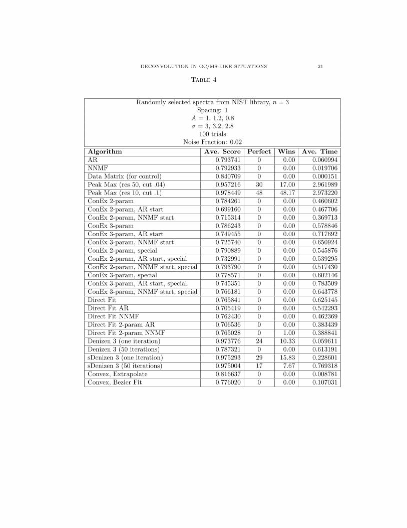
Table 4
Randomly selected spectra from NIST library, n = 3Spacing: 1
A = 1, 1.2, 0.8σ = 3, 3.2, 2.8
100 trialsNoise Fraction: 0.02
Algorithm Ave. Score Perfect Wins Ave. TimeAR 0.793741 0 0.00 0.060994NNMF 0.792933 0 0.00 0.019706Data Matrix (for control) 0.840709 0 0.00 0.000151Peak Max (res 50, cut .04) 0.957216 30 17.00 2.961989Peak Max (res 10, cut .1) 0.978449 48 48.17 2.973220ConEx 2-param 0.784261 0 0.00 0.460602ConEx 2-param, AR start 0.699160 0 0.00 0.467706ConEx 2-param, NNMF start 0.715314 0 0.00 0.369713ConEx 3-param 0.786243 0 0.00 0.578846ConEx 3-param, AR start 0.749455 0 0.00 0.717692ConEx 3-param, NNMF start 0.725740 0 0.00 0.650924ConEx 2-param, special 0.790889 0 0.00 0.545876ConEx 2-param, AR start, special 0.732991 0 0.00 0.539295ConEx 2-param, NNMF start, special 0.793790 0 0.00 0.517430ConEx 3-param, special 0.778571 0 0.00 0.602146ConEx 3-param, AR start, special 0.745351 0 0.00 0.783509ConEx 3-param, NNMF start, special 0.766181 0 0.00 0.643778Direct Fit 0.765841 0 0.00 0.625145Direct Fit AR 0.705419 0 0.00 0.542293Direct Fit NNMF 0.762430 0 0.00 0.462369Direct Fit 2-param AR 0.706536 0 0.00 0.383439Direct Fit 2-param NNMF 0.765028 0 1.00 0.388841Denizen 3 (one iteration) 0.973776 24 10.33 0.059611Denizen 3 (50 iterations) 0.787321 0 0.00 0.613191sDenizen 3 (one iteration) 0.975293 29 15.83 0.228601sDenizen 3 (50 iterations) 0.975004 17 7.67 0.769318Convex, Extrapolate 0.816637 0 0.00 0.008781Convex, Bezier Fit 0.776020 0 0.00 0.107031
22 DREW JOHNSON
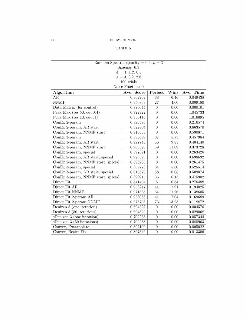
Table 5
Random Spectra, sparsity = 0.3, n = 3Spacing: 0.3A = 1, 1.2, 0.8σ = 3, 3.2, 2.8
100 trialsNoise Fraction: 0
Algorithm Ave. Score Perfect Wins Ave. TimeAR 0.962262 38 6.46 0.049438NNMF 0.950839 27 4.60 0.009180Data Matrix (for control) 0.876044 0 0.00 0.000101Peak Max (res 50, cut .04) 0.922922 0 0.00 1.045733Peak Max (res 10, cut .1) 0.930116 0 0.00 1.016095ConEx 2-param 0.896595 0 0.00 0.216574ConEx 2-param, AR start 0.922804 0 0.00 0.663570ConEx 2-param, NNMF start 0.910838 0 0.00 0.590871ConEx 3-param 0.893699 37 5.73 0.457984ConEx 3-param, AR start 0.927743 56 9.83 0.404140ConEx 3-param, NNMF start 0.903325 59 11.09 0.373728ConEx 2-param, special 0.897821 0 0.00 0.263426ConEx 2-param, AR start, special 0.923525 0 0.00 0.698692ConEx 2-param, NNMF start, special 0.895283 0 0.00 0.261475ConEx 3-param, special 0.869778 34 5.80 0.525514ConEx 3-param, AR start, special 0.910579 58 10.08 0.509074ConEx 3-param, NNMF start, special 0.890915 36 6.13 0.475902Direct Fit 0.841494 6 0.84 0.276488Direct Fit AR 0.953247 44 7.91 0.194025Direct Fit NNMF 0.971838 64 11.26 0.138605Direct Fit 2-param AR 0.953066 41 7.04 0.169689Direct Fit 2-param NNMF 0.975705 73 13.23 0.118872Denizen 3 (one iteration) 0.694322 0 0.00 0.004576Denizen 3 (50 iterations) 0.694322 0 0.00 0.029068sDenizen 3 (one iteration) 0.702238 0 0.00 0.057344sDenizen 3 (50 iterations) 0.702238 0 0.00 0.080963Convex, Extrapolate 0.892109 0 0.00 0.005022Convex, Bezier Fit 0.867346 0 0.00 0.013306