Introduction - polytechniquefusy/Articles/article_boundaries.pdf · every non-boundary face has...
42
BIJECTIONS FOR PLANAR MAPS WITH BOUNDARIES OLIVIER BERNARDI * AND ´ ERIC FUSY † Abstract. We present bijections for planar maps with boundaries. In particular, we obtain bijections for triangulations and quadrangulations of the sphere with boundaries of prescribed lengths. For triangulations we recover the beautiful factorized formula obtained by Krikun using a (technically involved) generating function approach. The analogous formula for quadrangulations is new. We also obtain a far-reaching generalization for other face-degrees. In fact, all the known enumerative formulas for maps with boundaries are proved bijectively in the present article (and several new formulas are obtained). Our method is to show that maps with boundaries can be endowed with certain “canonical” orientations, making them amenable to the master bijection approach we developed in previous articles. As an application of our enumerative formulas, we note that they provide an exact solution of the dimer model on rooted triangulations and quadrangulations. 1. Introduction In this article, we present bijections for planar maps with boundaries. Recall that a planar map is a decomposition of the 2-dimensional sphere into vertices, edges, and faces, considered up to continuous deformation (see precise definitions in Section 2). We deal exclusively with planar maps in this article and call them simply maps from now on. A map with boundaries is a map with a set of distinguished faces called boundary faces which are pairwise vertex-disjoint, and have simple-cycle contours (no pinch points). We call boundaries the contours of the boundary faces. We can think of the boundary faces as holes in the sphere, and maps with boundaries as a decomposition of a sphere with holes into vertices, edges and faces. A triangulation with boundaries (resp. quadrangulation with boundaries ) is a map with boundaries such that every non-boundary face has degree 3 (resp. 4). The main results obtained in this article are bijections for triangulations and quadrangulations with boundaries. The bijection establishes a correspondence between these maps and certain types of plane trees. This, in turns, easily yields factorized enumeration formulas with control on the number and lengths of the boundaries. In the case of triangulations, the enumerative formula had been established by Krikun [10] (by a technically involved “guessing/checking” generating function approach). The case of quadrangulations is new. We also present a far-reaching generalization for maps with other face-degrees. The strategy we apply is to adapt to maps with boundaries the “master bijection” approach we developed in [2, 3] for maps without boundaries. Roughly speaking, this strategy reduces the problem of finding bijections, to the problem of exhibiting canonical orientations characterizing these classes of maps. Let us now state the enumerative formulas derived from our bijections for triangulations and quadran- gulations. We call a map with boundaries multi-rooted if the r boundary faces are labeled with distinct numbers in [r]= {1,...,r}, and each one has a marked corner; see Figure 1. For m ≥ 0 and a 1 ,...,a r positive integers, we denote T (m; a 1 ,...,a r ) (resp. Q(m; a 1 ,...,a r )) the set of multi-rooted triangulations Date : December 14, 2017. * Department of Mathematics, Brandeis University, Waltham MA, USA, [email protected]. † LIX, ´ Ecole Polytechnique, Palaiseau, France, [email protected]. 1
-
Upload
nguyenlien -
Category
Documents
-
view
214 -
download
0
Transcript of Introduction - polytechniquefusy/Articles/article_boundaries.pdf · every non-boundary face has...
BIJECTIONS FOR PLANAR MAPS WITH BOUNDARIES
OLIVIER BERNARDI∗ AND ERIC FUSY†
Abstract. We present bijections for planar maps with boundaries. In particular, we obtain bijections fortriangulations and quadrangulations of the sphere with boundaries of prescribed lengths. For triangulations
we recover the beautiful factorized formula obtained by Krikun using a (technically involved) generatingfunction approach. The analogous formula for quadrangulations is new. We also obtain a far-reaching
generalization for other face-degrees. In fact, all the known enumerative formulas for maps with boundaries
are proved bijectively in the present article (and several new formulas are obtained).Our method is to show that maps with boundaries can be endowed with certain “canonical” orientations,
making them amenable to the master bijection approach we developed in previous articles. As an application
of our enumerative formulas, we note that they provide an exact solution of the dimer model on rootedtriangulations and quadrangulations.
1. Introduction
In this article, we present bijections for planar maps with boundaries. Recall that a planar map isa decomposition of the 2-dimensional sphere into vertices, edges, and faces, considered up to continuousdeformation (see precise definitions in Section 2). We deal exclusively with planar maps in this article andcall them simply maps from now on. A map with boundaries is a map with a set of distinguished facescalled boundary faces which are pairwise vertex-disjoint, and have simple-cycle contours (no pinch points).We call boundaries the contours of the boundary faces. We can think of the boundary faces as holes in thesphere, and maps with boundaries as a decomposition of a sphere with holes into vertices, edges and faces.A triangulation with boundaries (resp. quadrangulation with boundaries) is a map with boundaries such thatevery non-boundary face has degree 3 (resp. 4).
The main results obtained in this article are bijections for triangulations and quadrangulations withboundaries. The bijection establishes a correspondence between these maps and certain types of plane trees.This, in turns, easily yields factorized enumeration formulas with control on the number and lengths of theboundaries. In the case of triangulations, the enumerative formula had been established by Krikun [10] (bya technically involved “guessing/checking” generating function approach). The case of quadrangulations isnew. We also present a far-reaching generalization for maps with other face-degrees.
The strategy we apply is to adapt to maps with boundaries the “master bijection” approach we developedin [2, 3] for maps without boundaries. Roughly speaking, this strategy reduces the problem of findingbijections, to the problem of exhibiting canonical orientations characterizing these classes of maps.
Let us now state the enumerative formulas derived from our bijections for triangulations and quadran-gulations. We call a map with boundaries multi-rooted if the r boundary faces are labeled with distinctnumbers in [r] = 1, . . . , r, and each one has a marked corner; see Figure 1. For m ≥ 0 and a1, . . . , arpositive integers, we denote T (m; a1, . . . , ar) (resp. Q(m; a1, . . . , ar)) the set of multi-rooted triangulations
Date: December 14, 2017.∗Department of Mathematics, Brandeis University, Waltham MA, USA, [email protected].†LIX, Ecole Polytechnique, Palaiseau, France, [email protected].
1

2 O. BERNARDI AND E. FUSY
1
2
31
2
3
Figure 1. Left: a quadrangulation in Q[3; 4, 2, 6]. Right: a triangulation in T [3; 2, 1, 3].
(resp. quadrangulations) with r boundary faces, and m internal vertices (vertices not on the boundaries),such that the boundary labeled i has length ai for all i ∈ [r]. In 2007 Krikun proved the following result:
Theorem 1.1 (Krikun [10]). For m ≥ 0 and a1, . . . , ar positive integers,
(1) |T [m; a1, . . . , ar]| =4k(e− 2)!!
m!(2b+ k)!!
r∏i=1
ai
(2aiai
),
where b :=∑ri=1 ai is the total boundary length, k := r+m− 2, and e = 2b+ 3k is the number of edges (and
the notation n!! stands for∏b(n−1)/2ci=0 (n− 2i)).
We obtain a bijective proof of this result, and also prove the following analogue:
Theorem 1.2. For m ≥ 0 and a1, . . . , ar positive integers,
(2) |Q[m; 2a1, . . . , 2ar]| =3k(e− 1)!
m!(3b+ k)!
r∏i=1
2ai
(3aiai
),
where b :=∑ri=1 ai is the half-total boundary length, k := r+m− 2, and e = 3b+ 2k is the number of edges.
Equations (1) and (2) are generalizations of classical formulas. Indeed, the doubly degenerate case m = 0and r = 1 of (1) gives the well-known Catalan formula for the number of triangulations of a polygon without
interior points |T [0; a]| = Cat(a − 2) = (2a−4)!(a−1)!(a−2)! . Similarly, the case m = 0 and r = 1 of (2) gives the
2-Catalan formula for the number of quadrangulations of a polygon without interior points |Q[0; 2a]| =(3a−3)!
(a−1)!(2a−1)! . The case r = 1, a = 1 of (2) is already non-trivial as it gives the well-known formula for the
number of rooted quadrangulations with m+2 vertices (upon seeing the root-edge as blown into a boundaryface of degree 2):
|Q[m; 2]| = 2 · 3m(2m)!
m!(m+ 2)!.
More generally, the case r = 1 of (2) yields
|Q[m; 2a]| = 3m−1(3a+ 2m− 3)!
m!(3a+m− 1)!
(3a)!
(2a− 1)!a!,
which is the formula given in [6, Eq.(2.12)] for the number of rooted quadrangulations with one simpleboundary of length 2a, and m internal vertices. Similarly, the case r = 1 of (1) yields the formula for the

BIJECTIONS FOR PLANAR MAPS WITH BOUNDARIES 3
number of rooted triangulations with one simple boundary of length a, but it seems that this formula wasnot known prior to [10]. Lastly, in Section 5 we use the special case of (1) and (2) where all the boundarieshave length 2 in order to solve the dimer model on triangulations and quadrangulations.
As a side remark, let us discuss the counterparts of (1) and (2) when we remove the condition for the
boundaries to be simple and pairwise disjoint. Let T [n; a1, · · · , ar] (resp. Q[n; a1, . . . , ar]) be the set of mapswith n+ r faces, n faces of degree 3 (resp. 4) and r distinguished faces labeled 1, . . . , r of respective degreesa1, . . . , ar, each having a marked corner. It is easy to deduce from Tutte’s slicings formula [17] that
|Q[n; 2a1, . . . , 2ar]| =(e− 1)!
v!n!3n
r∏i=1
2a1
(2ai − 1
ai
),
where v = n + 2 +∑ri=1(ai − 1) is the total number of vertices, and e = 2n +
∑ri=1 ai is the total number
of edges. However no factorized formula should exist for |T [n; a1, . . . , ar]|, since the formula for r = 1 isalready complicated [11].
As mentioned above, we have also generalized our results to other face degrees. For these extensions,there is actually a necessary “girth condition” to take into account in order to obtain bijections. Precisely,we define a notion of internal girth for plane maps with boundaries. The internal girth coincides with thegirth1 when the map has at most one boundary (but can be larger than the girth in general). For any integerd ≥ 1, we obtain a bijection for maps with boundaries having internal girth d, and non-boundary faces ofdegrees in d, d + 1, d + 2 (with control on the number of faces of each degree). For d = 1, the internalgirth condition is void, and restricting the non-boundary faces to have degree d + 2 = 3 gives our resultfor triangulations with boundaries. For d = 2, the internal girth condition is void for bipartite maps, andrestricting the non-boundary faces to have degree d + 2 = 4 gives our result for bipartite quadrangulationswith boundaries. For the values of d ≥ 3, the case of a single boundary with all the internal faces of degreed corresponds to the results obtained in [2] (bijections for d-angulations of girth d ≥ 3 with at most oneboundary). For d = 2, the case of a single boundary with all the internal faces of degree 3 gives a bijectionfor loopless triangulations (i.e. triangulations of girth at least 2) with a single boundary and we recover thecounting formula of Mullin [12]. Hence, our bijections cover the cases of triangulations with a single boundarywith girth at least d, for d ∈ 1, 2, 3 (for girth 1 we give the first bijective proof, while for girth 2 the firstbijective proof was given in [13] and for girth 3 it was given in [14], and generalized to d-angulations in [1]).Furthermore, in Theorem 6.12 we give generalizations of these results in the form of multivariate factorizedcounting formulas, analogous to Krikun formula (1), for the classes of triangulations of internal girth d = 2and d = 3. Lastly, we give multivariate factorized counting formulas for the classes of quadrangulations ofinternal girth d = 4 thereby generalizing the formula of Brown [7] for simple quadrangulations with a singleboundary. In fact, all the known counting formulas for maps with boundaries are proved bijectively in thepresent article.
This article is organized as follows. In Section 2 we set our definitions about maps, and adapt the masterbijection established in [2] to maps with boundaries. In Section 3, we define canonical orientations forquadrangulations with boundaries, and obtain a bijection with a class of trees called mobiles (the case whereat least one boundary has size 2 is simpler, while the general case requires to first cut the map into twopieces). In Section 4 we treat similarly the case of triangulations. In Section 5, we count mobiles and obtain(1) and (2). We also derive from our formulas (both for coefficients and generating functions) exact solutionsof the dimer model on rooted quadrangulations and triangulations. In Section 6 we unify and extend theresults (orientations, bijections, and enumeration) to more general face-degree conditions. In Section 7, we
1We recall that the girth of a graph G is the length of a shortest cycle of edges in G.
4 O. BERNARDI AND E. FUSY
prove the existence and uniqueness of the needed canonical orientations for maps with boundaries. Lastly,in Section 8, we discuss additional results and perspectives.
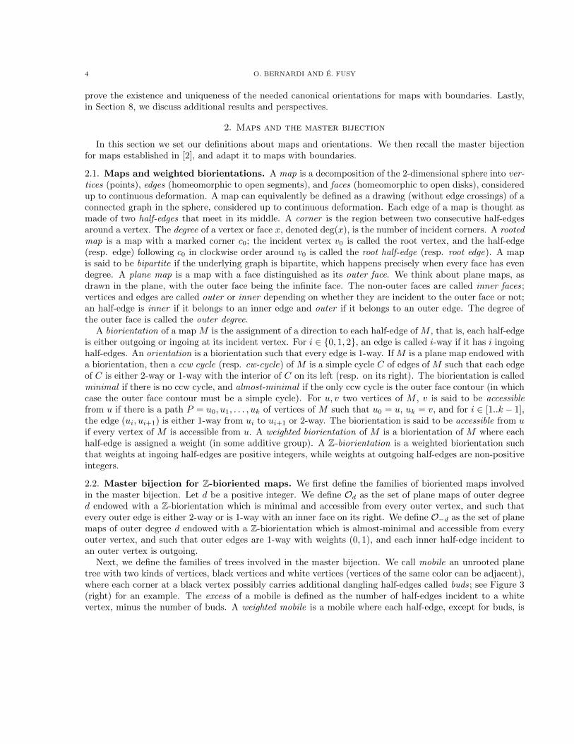
2. Maps and the master bijection
In this section we set our definitions about maps and orientations. We then recall the master bijectionfor maps established in [2], and adapt it to maps with boundaries.
2.1. Maps and weighted biorientations. A map is a decomposition of the 2-dimensional sphere into ver-tices (points), edges (homeomorphic to open segments), and faces (homeomorphic to open disks), consideredup to continuous deformation. A map can equivalently be defined as a drawing (without edge crossings) of aconnected graph in the sphere, considered up to continuous deformation. Each edge of a map is thought asmade of two half-edges that meet in its middle. A corner is the region between two consecutive half-edgesaround a vertex. The degree of a vertex or face x, denoted deg(x), is the number of incident corners. A rootedmap is a map with a marked corner c0; the incident vertex v0 is called the root vertex, and the half-edge(resp. edge) following c0 in clockwise order around v0 is called the root half-edge (resp. root edge). A mapis said to be bipartite if the underlying graph is bipartite, which happens precisely when every face has evendegree. A plane map is a map with a face distinguished as its outer face. We think about plane maps, asdrawn in the plane, with the outer face being the infinite face. The non-outer faces are called inner faces;vertices and edges are called outer or inner depending on whether they are incident to the outer face or not;an half-edge is inner if it belongs to an inner edge and outer if it belongs to an outer edge. The degree ofthe outer face is called the outer degree.
A biorientation of a map M is the assignment of a direction to each half-edge of M , that is, each half-edgeis either outgoing or ingoing at its incident vertex. For i ∈ 0, 1, 2, an edge is called i-way if it has i ingoinghalf-edges. An orientation is a biorientation such that every edge is 1-way. If M is a plane map endowed witha biorientation, then a ccw cycle (resp. cw-cycle) of M is a simple cycle C of edges of M such that each edgeof C is either 2-way or 1-way with the interior of C on its left (resp. on its right). The biorientation is calledminimal if there is no ccw cycle, and almost-minimal if the only ccw cycle is the outer face contour (in whichcase the outer face contour must be a simple cycle). For u, v two vertices of M , v is said to be accessiblefrom u if there is a path P = u0, u1, . . . , uk of vertices of M such that u0 = u, uk = v, and for i ∈ [1..k − 1],the edge (ui, ui+1) is either 1-way from ui to ui+1 or 2-way. The biorientation is said to be accessible from uif every vertex of M is accessible from u. A weighted biorientation of M is a biorientation of M where eachhalf-edge is assigned a weight (in some additive group). A Z-biorientation is a weighted biorientation suchthat weights at ingoing half-edges are positive integers, while weights at outgoing half-edges are non-positiveintegers.
2.2. Master bijection for Z-bioriented maps. We first define the families of bioriented maps involvedin the master bijection. Let d be a positive integer. We define Od as the set of plane maps of outer degreed endowed with a Z-biorientation which is minimal and accessible from every outer vertex, and such thatevery outer edge is either 2-way or is 1-way with an inner face on its right. We define O−d as the set of planemaps of outer degree d endowed with a Z-biorientation which is almost-minimal and accessible from everyouter vertex, and such that outer edges are 1-way with weights (0, 1), and each inner half-edge incident toan outer vertex is outgoing.
Next, we define the families of trees involved in the master bijection. We call mobile an unrooted planetree with two kinds of vertices, black vertices and white vertices (vertices of the same color can be adjacent),where each corner at a black vertex possibly carries additional dangling half-edges called buds; see Figure 3(right) for an example. The excess of a mobile is defined as the number of half-edges incident to a whitevertex, minus the number of buds. A weighted mobile is a mobile where each half-edge, except for buds, is
BIJECTIONS FOR PLANAR MAPS WITH BOUNDARIES 5
assigned a weight. A Z-mobile is a weighted mobile such that weights of half-edges incident to white verticesare positive integers, while weights at half-edges incident to black vertices are non-positive integers. Ford ∈ Z, we denote by Bd the set of Z-mobiles of excess d.
⇓w
w′
ww′
⇓w
w′
ww′
⇓w
w′
w
w′
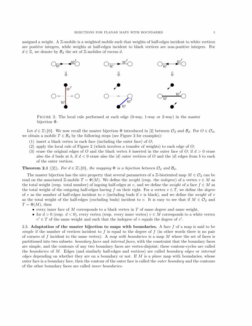
Figure 2. The local rule performed at each edge (0-way, 1-way or 2-way) in the masterbijection Φ.
Let d ∈ Z\0. We now recall the master bijection Φ introduced in [2] between Od and Bd. For O ∈ Od,we obtain a mobile T ∈ Bd by the following steps (see Figure 3 for examples):
(1) insert a black vertex in each face (including the outer face) of O;(2) apply the local rule of Figure 2 (which involves a transfer of weights) to each edge of O;(3) erase the original edges of O and the black vertex b inserted in the outer face of O; if d > 0 erase
also the d buds at b, if d < 0 erase also the |d| outer vertices of O and the |d| edges from b to eachof the outer vertices.
Theorem 2.1 ([2]). For d ∈ Z\0, the mapping Φ is a bijection between Od and Bd.
The master bijection has the nice property that several parameters of a Z-bioriented map M ∈ Od can beread on the associated Z-mobile T = Φ(M). We define the weight (resp. the indegree) of a vertex v ∈M asthe total weight (resp. total number) of ingoing half-edges at v, and we define the weight of a face f ∈M asthe total weight of the outgoing half-edges having f on their right. For a vertex v ∈ T , we define the degreeof v as the number of half-edges incident to v (including buds if v is black), and we define the weight of vas the total weight of the half-edges (excluding buds) incident to v. It is easy to see that if M ∈ Od andT = Φ(M), then
• every inner face of M corresponds to a black vertex in T of same degree and same weight,• for d > 0 (resp. d < 0), every vertex (resp. every inner vertex) v ∈M corresponds to a white vertexv′ ∈ T of the same weight and such that the indegree of v equals the degree of v′.
2.3. Adaptation of the master bijection to maps with boundaries. A face f of a map is said to besimple if the number of vertices incident to f is equal to the degree of f (in other words there is no pairof corners of f incident to the same vertex). A map with boundaries is a map M where the set of faces ispartitioned into two subsets: boundary faces and internal faces, with the constraint that the boundary facesare simple, and the contours of any two boundary faces are vertex-disjoint; these contour-cycles are calledthe boundaries of M . Edges (and similarly half-edges and vertices) are called boundary edges or internaledges depending on whether they are on a boundary or not. If M is a plane map with boundaries, whoseouter face is a boundary face, then the contour of the outer face is called the outer boundary and the contoursof the other boundary faces are called inner boundaries.

6 O. BERNARDI AND E. FUSY
-2-5
21
-14 -3
0
-1
23
1
0
1
-3
2
0
0
0
1
1
1
10
⇒ ⇒-2
-5
0
-3
2-1
4-1
3
12 -3
01
21
⇒ ⇒
2
2
3
3
1
1
1
0
-3-2
4
-1
-5
3
0
-1
0
1
2-4
2
3
3
0
1
2
1
0
1-5
2
4
0
-1
1-4
-2
-3
-13
Figure 3. The master bijection from a Z-bioriented plane map in Od to a Z-mobile ofexcess d (the top example has d = −4, the bottom-example has d = 5).
For M a map with boundaries, a Z-biorientation of M is called consistent if the boundary edges are all1-way with weights (0, 1) and have the incident boundary face on their right. For d ∈ Z\0, we denote by
Od the set of plane maps with boundaries endowed with a consistent Z-biorientation, such that the outer faceis a boundary face for d < 0 and an internal face for d > 0, and when forgetting which faces are boundaryfaces, the underlying Z-bioriented plane map is in Od.
A boundary mobile is a mobile where every corner at a white vertex might carry additional dangling half-edges called legs. White vertices having at least one leg are called boundary vertices. The degree of a whitevertex v is the number of non-leg half-edges incident to v. The excess of a boundary mobile is defined as thenumber of half-edges incident to a white vertex (including the legs) minus the number of buds. A boundaryZ-mobile is a boundary mobile where the half-edges different from buds and legs carry weights in Z suchthat half-edges at white vertices have positive weights while half-edges at black vertices have non-positive
weights. For d ∈ Z, we denote by Bd the set of boundary Z-mobiles of excess d.
We can now specialize the master bijection. For O ∈ Od, let T = Φ(O) be the associated Z-mobile. Notethat each inner boundary face f of O of degree k yields a black vertex v of degree k in T such that v has nobud, and the k neighbors w1, . . . , wk of v are the white vertices corresponding to the vertices around f . Weperform the following operation represented in Figure 4: we insert one leg at each corner of v, then contract

BIJECTIONS FOR PLANAR MAPS WITH BOUNDARIES 7
. . .
. . .
. . .. . .
. . .
. . .
. . .
. . .. . .
. . .
(a) (b)
=⇒v
Figure 4. Reduction operation at the black vertex v corresponding to an inner boundary
face in O ∈ Od.
the edges incident to v, and finally recolor b as white. Doing this for each inner boundary we obtain (withoutloss of information) a boundary Z-mobile T ′ of the same excess as T , called the reduction of T . We denote
by Φ the mapping such that Φ(O) = T ′.We now argue that Φ is a bijection between Od and Bd. For a boundary mobile T ′, the expansion of T ′
is the mobile T obtained from T ′ by applying to every boundary vertex the process of Figure 4 in reversedirection: a boundary vertex with k legs yields in T a distinguished black vertex of degree k with no buds,and with only white neighbors. Note that, if T ′ has non-zero excess d and if O ∈ Od denotes the Z-biorientedplane map associated to T by the master bijection, then each distinguished face f ∈ O (i.e., a face associatedto a distinguished black vertex of T ) is simple; indeed if k ≥ 1 denotes the degree of f , the correspondingblack vertex v ∈ T has k white neighbors, which thus correspond to k distinct vertices incident to f . Inaddition the contours of the distinguished inner faces are disjoint since the expansions of any two distinctboundary vertices of T ′ are vertex-disjoint in T . Lastly, for d ∈ Z∗−, the outer face is simple and disjointfrom the contours of the inner distinguished faces (indeed the vertices around an inner distinguished face of
O are all present in T , hence are inner vertices of O). We thus conclude that O belongs to Od, upon seeingthe distinguished faces (including the outer face for d ∈ Z∗−) as boundary faces. The following statementsummarizes the previous discussion:
Theorem 2.2. The master bijection Φ adapted to consistent Z-biorientations is a bijection between Od and
Bd for each d ∈ Z\0.
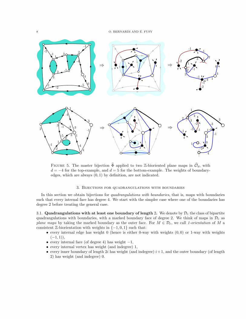
The bijection Φ is illustrated in Figure 5. As before, several parameters can be tracked through thebijection. For a map M with boundaries endowed with a consistent Z-biorientation, we define the weight(resp. the indegree) of a boundary C as the total weight (resp. total number) of ingoing half-edges incidentto a vertex of C but not lying on an edge of C. For a boundary Z-mobile, we define the weight of a white
vertex v as the total weight of the half-edges (excluding legs) incident to v. It is easy to see that if O ∈ Odand T = Φ(O), then
• every internal inner face of O corresponds to a black vertex in T of same degree and same weight,• every internal vertex v ∈ O corresponds to a non-boundary white vertex v′ ∈ T of the same weight
and such that the indegree of v equals the degree of v′,• every inner boundary of length k, indegree r, and weight j in O corresponds to a boundary vertex
in T with k legs, degree r, and weight j.
8 O. BERNARDI AND E. FUSY
⇒ ⇒
⇒ ⇒
-23
1
2-1
-4
1
-5-2
-1
2
-1
3 4
0
-1
-2
-1
3
1
3-1
-4 1
4
0
-1
2
2 -1
-1
23
-5
-3
4
1
3
-1
4-2
10
3
-1 -2
-4
1
3
1
4
-3
1 -4
-1
4
3
01
-2
2
-1
3
-5 -1
-2
-5-2
Figure 5. The master bijection Φ applied to two Z-bioriented plane maps in Od, withd = −4 for the top-example, and d = 5 for the bottom-example. The weights of boundary-edges, which are always (0, 1) by definition, are not indicated.
3. Bijections for quadrangulations with boundaries
In this section we obtain bijections for quadrangulations with boundaries, that is, maps with boundariessuch that every internal face has degree 4. We start with the simpler case where one of the boundaries hasdegree 2 before treating the general case.
3.1. Quadrangulations with at least one boundary of length 2. We denote by D3 the class of bipartitequadrangulations with boundaries, with a marked boundary face of degree 2. We think of maps in D3 asplane maps by taking the marked boundary as the outer face. For M ∈ D3, we call 1-orientation of M aconsistent Z-biorientation with weights in −1, 0, 1 such that:
• every internal edge has weight 0 (hence is either 0-way with weights (0, 0) or 1-way with weights(−1, 1)),
• every internal face (of degree 4) has weight −1,• every internal vertex has weight (and indegree) 1,• every inner boundary of length 2i has weight (and indegree) i+1, and the outer boundary (of length
2) has weight (and indegree) 0.

BIJECTIONS FOR PLANAR MAPS WITH BOUNDARIES 9
Proposition 3.1. Every map M ∈ D3 has a unique 1-orientation in O−2. We call it its canonical biorien-tation.
The proof of Proposition 3.1 is delayed to Section 7. We denote by T3 the set of boundary mobilesassociated to maps in D3 (endowed with their canonical biorientation) via the master bijection for mapswith boundaries. By Theorem 2.2, these are the boundary mobiles with weights in −1, 0, 1 satisfying thefollowing properties:
• every edge has weight 0 (hence, is either black-black of weights (0, 0), or black-white of weights(−1, 1)),• every black vertex has degree 4 and weight −1 (hence has a unique white neighbor),• for all i ≥ 0, every white vertex of degree i+ 1 carries 2i legs.
We omit the condition that the excess is −2, because it can easily be checked to be a consequence of theabove properties.
(a) (b) (c)
Figure 6. (a) A map in D3 endowed with its canonical biorientation (the 1-way edgesare indicated as directed edges, the 0-way edges are indicated as undirected edges, andthe weights, which are uniquely induced by the biorientation, are not indicated). (b) Thequadrangulation superimposed with the corresponding mobile. (c) The reduced boundarymobile (with 2i legs at each white vertex of degree i + 1), where again the weights (whichare uniquely induced by the mobile) are not indicated.
To summarize, Theorem 2.2 and Proposition 3.1 yield the following bijection (illustrated in Figure 6) forbipartite quadrangulations with a distinguished boundary of length 2.
Theorem 3.2. The set D3 of quadrangulations with boundaries is in bijection with the set T3 of Z-mobiles
via the master bijection Φ. If M ∈ D3 and T ∈ T3 are associated by the bijection, then each inner boundaryof length 2i in M corresponds to a white vertex in T of weight (and degree) i + 1, and each internal vertexof M corresponds to a white leaf in T .

10 O. BERNARDI AND E. FUSY
3.2. Quadrangulations with arbitrary boundary lengths. For a ≥ 1, we denote by D(2a)3 the set of
bipartite quadrangulations with boundaries with a marked boundary face of degree 2a. In the previous
section we obtained a bijection for D(2)3 = D3. In order to get a bijection for D(2a)
3 when a > 1, we will needto first mark an edge and decompose our marked maps into two pieces before applying the master bijectionto each piece2.
Let D(2a)3 be the set of maps obtained from maps in D(2a)
3 by also marking an edge (either an internal
edge or a boundary edge). Let A(2a)3 be the set of bipartite maps with a marked boundary face of degree 2a
and a marked internal face of degree 2, such that all the non-marked internal faces have degree 4. We also
denote by ~A(2a)3 the set of maps obtained from maps in A(2a)
3 by marking a corner in the marked boundaryface.
Given a map M in D(2a)3 , we obtain a map M ′ in A(2a)
3 by opening the marked edge into an internal faceof degree 2. This operation, which we call edge-opening is clearly a bijection for a > 1:
Lemma 3.3. For all a > 1, the edge-opening is a bijection between D(2a)3 and A(2a)
3 which preserves thenumber of internal vertices and the boundary lengths.
Note however that A(2)3 contains a map ε with 2 edges (a 2-cycle separating a boundary and an internal
face) which is not obtained from a map in D(2)3 , so that the bijection is between D(2)
3 and A(2)3 \ ε.
We will now describe a canonical decomposition of maps in A(2a)3 illustrated in Figure 7(a)-(b). Let M be
in A(2a)3 , and let fs be the marked boundary face. Let C be a simple cycle of M , and let RC and LC be the
regions bounded by C containing fs and not containing fs respectively. The cycle C is said to be blockingif C has length 2, the marked internal face is in LC , and any boundary face incident to a vertex of C is inRC . Note that the contour of the marked internal face is a blocking cycle. It is easy to see that there existsa unique blocking cycle C such that LC is maximal (that is, contains LC′ for any blocking cycle C ′). Wecall C the maximal blocking cycle of M . The maximal blocking cycle is indicated in Figure 7(a). The mapM is called reduced if its maximal blocking cycle is the contour of the marked internal face, and we denote
by B(2a)3 and ~B(2a)
3 the subsets of A(2a)3 and ~A(2a)
3 corresponding to reduced maps.
We now consider the two maps obtained from a map M in A(2a)3 by “cutting the sphere” along the
maximal blocking cycle C, as illustrated in Figure 7(b). Precisely, we denote by M1 the map obtained fromM by replacing RC by a single marked boundary face (of degree 2), and we denote by M2 the map obtained
from M by replacing LC by a single marked internal face (of degree 2). It is clear that M1 is in A(2)3 , while
M2 is in B(2a)3 . Conversely, if we glue the marked boundary face of a map N1 ∈ A(2)
3 to the marked internal
face of a reduced map N2 ∈ B(2a)3 , we obtain a map M ∈ A(2a)
3 whose maximal blocking cycle is the contourof the glued faces, so that N1 = M1 and N2 = M2. In order to make the preceding decomposition bijective,
it is convenient to work with rooted maps. Given a map M in ~A(2a)3 , we define M1 and M2 as above, except
that we mark a corner in the newly created boundary face of M1. In order to fix a convention, we choosethe corner of M1 such that the vertices incident to the marked corners of M1 and M2 are in the same blockof the bipartition of the vertices of M . The decomposition M 7→ (M1,M2) is now bijective and we call it
the canonical decomposition of the maps in ~A(2a)3 . We summarize the above discussion:
Lemma 3.4. For all a ≥ 1, the canonical decomposition is a bijection between ~A(2a)3 and ~A(2)
3 × ~B(2a)3 .
Note that the case a = 1 above is special in that the set ~B(2)3 contains only the map ε.
2A similar strategy was already used in [2, 3, 4].

BIJECTIONS FOR PLANAR MAPS WITH BOUNDARIES 11
(a) (b) (c) (d)
inside C
outside C
CC
C
M2 ∈ B(4)3
M1 ∈ A(2)3
M ∈ A(4)3
fs
fs
Figure 7. (a) A map in A(4)3 : the marked boundary face is the outer face, the marked
internal face is indicated by a square, and the maximal blocking cycle C is drawn in bold.(b) The maps M1 and M2 resulting from cutting M along C, each represented as a planemap endowed with its canonical biorientation (the marked inner face in each case is indicatedby a square). (c) The mobiles associated to M1 and M2. (d) The reduced boundary mobilesassociated to M1 and M2, where the marked vertex (corresponding to the marked innerface) is indicated by a square.
Next, we describe bijections for maps in ~A(2)3 and ~B(2a)
3 by using a “master bijection” approach illustrated
in Figure 7(b)-(d). For M ∈ A(2)3 , we call 1-orientation of M a consistent Z-biorientation of M with weights
in −1, 0, 1 such that:• every internal edge has weight 0,• every internal vertex has indegree 1,• every non-marked internal face (of degree 4) has weight −1, while the marked internal face (of degree
2) has weight 0,• every non-marked boundary of length 2i has weight (and indegree) i+1, while the marked boundary
(of length 2) has weight (and indegree) 0.
Proposition 3.5. Let M be a map in A(2)3 considered as a plane map by taking the outer face to be the
marked boundary face. Then M admits a unique 1-orientation in O−2. We call it the canonical biorientationof M .
Proof. This is a corollary of Proposition 3.1. Indeed, seeing M as a map D in D3 where an edge e is openedinto an internal face f1 of degree 2, the canonical biorientation of M is directly derived from the canonicalbiorientation of D, using the rules shown in Figure 8.
For M ∈ A(2a)3 , we call 1-orientation of M a consistent Z-biorientation with weights in −1, 0, 1 such
that:
12 O. BERNARDI AND E. FUSY
⇒0
0 0
0 0
0⇒
1
-1 0
0
-1
1⇒
1
0
0 1
0 0f1 f1 f1
Figure 8. Transferring the biorientations and weights when blowing an edge into an inter-nal face of degree 2.
• every internal edge has weight 0,• every internal vertex has weight (and indegree) 1,• every non-marked internal face (of degree 4) has weight −1, while the marked internal face (of degree
2) has weight 0,• every non-marked boundary of length 2i has weight (and indegree) i+1, while the marked boundary
(of length 2a) has weight (and indegree) a− 1.
Proposition 3.6. Let M be a map in A(2a)3 considered as a plane map by taking the outer face to be the
marked internal face. Then M has a 1-orientation in O2 if and only if it is reduced (i.e., is in B(2a)3 ). In
this case, M has a unique 1-orientation in O2. We call it the canonical biorientation of M .
The proof of Proposition 3.6 is delayed to Section 7. We denote by U3 the set of mobiles corresponding
to (canonically oriented) maps in A(2)3 via the master bijection. By Theorem 2.2, these are the boundary
Z-mobiles with weights in −1, 0, 1 satisfying the following properties (which imply that the excess is −2):• every edge has weight 0 (hence, is either black-black of weights (0, 0), or black-white of weights
(−1, 1)),• every black vertex has degree 4 and weight −1 (hence has a unique white neighbor), except for a
unique black vertex of degree 2 and weight 0,• for all i ≥ 0, every white vertex of degree i+ 1 carries 2i legs.
We also denote ~U3 the set of mobiles obtained from mobiles in U3 by marking one of the corners of the blackvertex of degree 2.
For a ≥ 1, we denote by V(2a)3
the set of mobiles corresponding to (canonically oriented) maps in B(2a)3 .
These are the boundary Z-mobiles with weights in −1, 0, 1 satisfying the following properties (which implythat the excess is 2):
• every edge has weight 0 (hence is either black-black of weights (0, 0), or black-white of weights(−1, 1)),
• every black vertex has degree 4 and weight −1 (hence has a unique white neighbor),• there is a marked white vertex of degree a− 1 which carries 2a legs,• for all i ≥ 0, every non-marked white vertex of degree i+ 1 carries 2i legs.
We also denote ~V(2a)3
the set of rooted mobiles obtained from from mobiles in V(2a)3
by marking one of the2a legs of the marked white vertex.
Propositions 3.5 and 3.6 together with the master bijection (Theorem 2.2) and Lemma 3.4 finally give:
Theorem 3.7. The set A(2)3 (resp. ~A(2)
3 ) of quadrangulations is in bijection with the set U3 (resp. ~U3) of
Z-mobiles. Similarly, for all a ≥ 1, the set B(2a)3 (resp. ~B(2a)
3 ) of quadrangulations is in bijection with the
set V(2a)3
(resp. ~V(2a)3
) of Z-mobiles.

BIJECTIONS FOR PLANAR MAPS WITH BOUNDARIES 13
Finally, the set ~A(2a)3 of quadrangulations is in bijection with the set ~U3 × ~V(2a)
3of pairs of Z-mobiles.
The bijection is such that if the map M corresponds to the pair of Z-mobiles (U, V ), then each non-markedboundary of length 2i in M corresponds to a non-marked white vertex of U ∪ V of weight (and degree) i+ 1,and each internal vertex of M corresponds to a non-marked white leaf of U ∪ V .
Theorem 3.7 is illustrated in Figure 7.
4. Bijections for triangulations with boundaries
In this section we adapt the strategy of Section 3 to triangulations with boundaries, that is, maps withboundaries such that every internal face has degree 3. We start with the simpler case where one of theboundaries has degree 1 before treating the general case.
4.1. Triangulations with at least one boundary of length 1. Let DM be the set of triangulations withboundaries, with a marked boundary face of degree 1. We think of maps in DM as plane maps by taking themarked boundary as the outer face. For M ∈ DM, we call 1-orientation of M a consistent Z-biorientationwith weights in −2,−1, 0, 1 and with the following properties:
• every internal edge has weight −1 (i.e., is either 0-way of weights (−1, 0), or 1-way of weights (−2, 1)),• every internal vertex has weight 1,• every internal face has weight −2,• every inner boundary of length i has weight (and indegree) i+1, and the outer boundary has weight 0.
Similarly as in Section 3.1 we have the following proposition proved in Section 7.
Proposition 4.1. Every M ∈ DM has a unique 1-orientation in O−1. We call it the canonical biorientationof M .
We denote by TM the set of mobiles corresponding to (canonically oriented) maps in DM via the masterbijection. By Theorem 2.2, these are the boundary Z-mobiles satisfying the following properties (whichreadily imply that the weights are in −2,−1, 0, 1, and the excess is −1):
• every edge has weight −1 (hence is either black-black of weights (−1, 0), or is black-white of weights(−2, 1)),
• every black vertex has degree 3 and weight −2,• for all i ≥ 0, every white vertex of degree i+ 1 carries i legs.
To summarize, we obtain the following bijection for triangulations with a boundary of length 1 (seeFigure 9 for an example):
Theorem 4.2. The set DM is in bijection with the set TM via the master bijection. If M ∈ DM and T ∈ TMare associated by the bijection, then each inner boundary of length i in M corresponds to a white vertex inT of degree i+ 1, and each internal vertex of M corresponds to a white leaf in T .
4.2. Triangulations with arbitrary boundary lengths. We now adapt the approach of Section 3.2
(decomposing maps into two pieces) to triangulations. For a ≥ 1, we denote by D(a)M the set of triangulations
with boundaries with a marked boundary face of degree a. We denote by D(a)M the set of maps obtained
from maps in D(a)M by also marking an arbitrary half-edge (either boundary or internal). We denote by A(a)
Mthe set of maps with boundaries having a marked boundary face of degree a and a marked internal face of
degree 1, such that all the non-marked internal faces have degree 3. Lastly, we denote ~A(a)M the set of maps
obtained from A(2a)M by marking a corner in the marked boundary face.
Given a map M in D(a)M , we obtain a map M ′ in A(a)
M by the operation illustrated in Figure 10, which wecall half-edge-opening. In words, we “open” the edge containing the marked half-edge h into a face f , and
14 O. BERNARDI AND E. FUSY
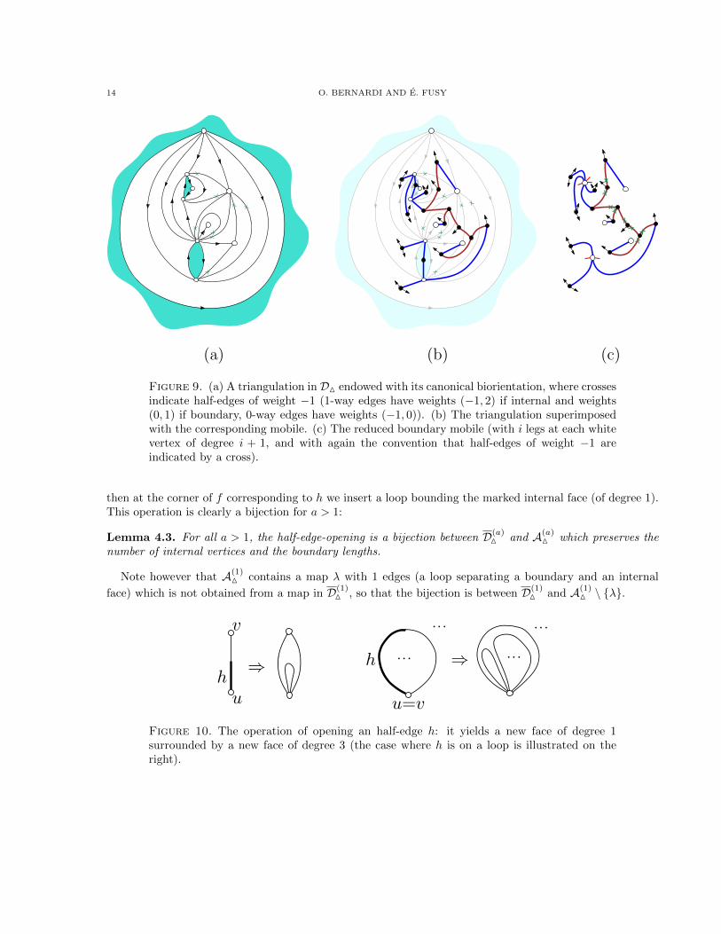
(a) (b) (c)
Figure 9. (a) A triangulation in DM endowed with its canonical biorientation, where crossesindicate half-edges of weight −1 (1-way edges have weights (−1, 2) if internal and weights(0, 1) if boundary, 0-way edges have weights (−1, 0)). (b) The triangulation superimposedwith the corresponding mobile. (c) The reduced boundary mobile (with i legs at each whitevertex of degree i + 1, and with again the convention that half-edges of weight −1 areindicated by a cross).
then at the corner of f corresponding to h we insert a loop bounding the marked internal face (of degree 1).This operation is clearly a bijection for a > 1:
Lemma 4.3. For all a > 1, the half-edge-opening is a bijection between D(a)M and A(a)
M which preserves thenumber of internal vertices and the boundary lengths.
Note however that A(1)M contains a map λ with 1 edges (a loop separating a boundary and an internal
face) which is not obtained from a map in D(1)M , so that the bijection is between D(1)
M and A(1)M \ λ.
⇒ ⇒h
h
u
v
u=v
Figure 10. The operation of opening an half-edge h: it yields a new face of degree 1surrounded by a new face of degree 3 (the case where h is on a loop is illustrated on theright).

BIJECTIONS FOR PLANAR MAPS WITH BOUNDARIES 15
Next, we describe a canonical decomposition of maps in A(a)M illustrated in Figure 11(a)-(b). For a cycle
C of a map M ∈ A(a)M , we denote by RC and LC the regions bounded by C containing and not containing
the marked boundary face fs respectively. The cycle C is said to be blocking if C has length 1 (that is, isa loop), the marked internal face is in LC , and any boundary face incident to a vertex of C is in RC . Notethat the contour of the marked internal face is a blocking cycle. It is easy to see that there exists a uniqueblocking cycle C such that LC is maximal (that is, contains LC′ for any blocking cycle C ′). We call C themaximal blocking cycle of M . The maximal blocking cycle is indicated in Figure 11(a). The map M is called
reduced if its maximal blocking cycle is the contour of the marked internal face, and we denote by B(a)M and
~B(a)M the subsets of A(a)
M and ~A(a)M corresponding to reduced maps.
inside C
outside CC
C
C
(a) (b) (c) (d)
M2 ∈ B(3)M
M1 ∈ A(2)M
M ∈ A(3)M
fs
Figure 11. (a) A map in A(3)M : the marked boundary face is the outer face, the marked
internal face is indicated by a square, and the maximal blocking cycle C is drawn in bold. (b)The maps M1 and M2 resulting from cutting M along C, each represented as a plane mapendowed with its canonical biorientation (the marked inner face in each case is indicatedby a square, each directed edge has weights (−2, 1) and each undirected edge has weights(−1, 0), with a cross on the half-edge of weight −1). (c) The mobiles associated to M1 andM2. (d) The reduced boundary mobiles associated to M1 and M2, where the marked vertexis represented by a square. Black-white edges have weights (−2, 1), and black-black edgeshave weights (−1, 0), with a cross on the half-edge of weight −1.
We now consider the two maps obtained from a map M in A(a)M by cutting the sphere along the maximal
blocking cycle C, as illustrated in Figure 11(b). Precisely, we denote by M1 the map obtained from M byreplacing RC by a single marked boundary face (of degree 1), and we denote by M2 the map obtained from
M by replacing LC by a single marked internal face (of degree 1). It is clear that M1 is in A(1)M , while
16 O. BERNARDI AND E. FUSY
M2 is in B(a)M . The decomposition M 7→ (M1,M2) is bijective (both for rooted and unrooted maps because
~A(1)M ' A(1)
M ), and we call it the canonical decomposition of maps in ~A(a)M . We summarize:
Lemma 4.4. For all a ≥ 1, the canonical decomposition is a bijection between ~A(a)M and A(1)
M × ~B(a)M .
Next, we describe bijections for maps inA(1)M and B(a)
M by using the master bijection approach, as illustrated
in Figure 11(b)-(d). For M ∈ A(1)M , we call 1-orientation of M a consistent Z-biorientation of M with weights
in −2,−1, 0, 1 such that:• every internal edge has weight −1,• every internal vertex has weight (and indegree) 1,• every non-marked internal face (of degree 3) has weight −2, and the marked internal face (of degree
1) has weight 0,• every non-marked boundary of length i has weight (and indegree) i + 1, and the marked boundary
has weight (and indegree) 0.The following result easily follows from Proposition 4.1 (similarly as Proposition 3.5 follows from Propo-
sition 3.1).
Proposition 4.5. Let M be a map in A(1)M , considered as a plane map by taking the marked boundary face
as the outer face. Then M admits a unique 1-orientation in O−1. We call it the canonical biorientation ofM .
For M ∈ A(a)M we call 1-orientation of M a consistent Z-biorientation with weights in −2,−1, 0, 1 such
that:• every internal edge has weight −1,• every internal vertex has weight (and indegree) 1,• every internal inner face (of degree 3) has weight −2, and the internal outer face (of degree 1) has
weight 0.• every non-marked boundary of length i has weight (and indegree) i+ 1, while the marked boundary
of length a, has weight (and indegree) a− 1.
Proposition 4.6. Let M be a map in A(a)M considered as a plane map by taking the outer face to be the
marked internal face. Then M has a 1-orientation in O1 if and only if it is reduced (i.e., is in B(a)M ). In this
case, M has a unique 1-orientation in O1, which we call the canonical biorientation of M .
Again the proof is delayed to Section 7.
We denote by UM the set of mobiles corresponding to (canonically oriented) maps in A(1)M via the master
bijection. These are the boundary Z-mobiles with weights in −2,−1, 0, 1 satisfying the following properties(which imply that the excess is −1):
• every internal edge has weight −1 (hence is either black-black of weights (−1, 0), or black-white ofweights (−2, 1)),
• every black vertex has degree 3 and weight −2, except for a unique black vertex of degree 1 andweight 0,
• for all i ≥ 0, every white vertex of degree i+ 1 carries i legs.
For a ≥ 1, we denote by V(a)M the set of mobiles corresponding to (canonically oriented) maps in B(a)
M . Theseare the boundary Z-mobiles with weights in −2,−1, 0, 1 satisfying the following properties (which implythat the excess is 1):
• every internal edge has weight −1• every black vertex has degree 3 and weight −2,
BIJECTIONS FOR PLANAR MAPS WITH BOUNDARIES 17
• there is a marked white vertex of degree a− 1 which carries a legs,• for all i ≥ 0, every non-marked white vertex of degree i+ 1 carries i legs.
We also denote ~V(a)M the set of mobiles obtained from from mobiles in V(a)
M by marking one of the a legs ofthe marked white vertex. Propositions 3.5 and 4.6 together with the master bijection (Theorem 2.2) andLemma 4.4 finally give:
Theorem 4.7. The set A(1)M of triangulations is in bijection with the set UM of Z-mobiles. For all a ≥ 1, the
set B(a)M (resp. ~B(a)
M ) of triangulations is in bijection with the set V(a)M (resp. ~V(a)
M ) of Z-mobiles. Finally the
set ~A(a)M of triangulations is in bijection with the set UM × ~V(a)
M of pairs of Z-mobiles. The bijection is suchthat if the map M corresponds to the pair of Z-mobiles (U, V ), then each non-marked boundary of length iin M corresponds to a non-marked white vertex in U ∪ V of weight (and degree) i + 1, and each internalvertex of M corresponds to a non-marked white leaf in U ∪ V .
Theorem 4.7 is illustrated in Figure 11.
5. Counting results
5.1. Proof of Theorem 1.2 for quadrangulations with boundaries. We define a planted mobile ofquadrangulated type as a tree P obtained as one of the two connected components after cutting a mobileT ∈ T3 in the middle of an edge e; the half-edge h of e that belongs to P is called the root half-edge of P ,and the vertex incident to h is called the root-vertex of P . The root-weight of P is the weight of h in T . Forj ∈ −1, 0, 1, let Rj ≡ Rj(t; z0, z1, z2, . . .) be the generating function of planted mobiles of quadrangulatedtype having root-weight j, where t is conjugate to the number of buds, and zi is conjugate to the numberof white vertices of degree i + 1 (with 2i additional legs) for i ≥ 0. We also denote R := t + R0. Thedecomposition of planted trees at the root easily implies that the series R−1, R0, R1 are determined by thefollowing system
(3)
R−1 = R3,R0 = 3R1R
2,
R1 =∑i≥0 zi
(3ii
)R−1
i,
where (for instance) the factor(
3ii
)in the 3rd line accounts for the number of ways to place the 2i legs
when the root-vertex has degree i+ 1 (the root half-edge plus i children), and the factor 3 in the second lineaccounts for choosing which of the 3 children of the root-vertex is white.
This gives R = t+ 3∑i≥0 zi
(3ii
)R3i+2, or equivalently,
(4) R = tφ(R), with φ(y) =(
1− 3∑i≥0
zi
(3i
i
)y3i+1
)−1
.
Let U3 ≡ U3(t; z0, z1, . . .) be the generating function of mobiles in ~U3 with t conjugate to the number ofbuds and zi conjugate to the number of white vertices of degree i + 1 for i ≥ 0. For a ≥ 1, let V (2a)
3≡
V (2a)3
(t; z0, z1, . . .) be the generating function of mobiles in ~V(2a)3
with t conjugate to the number of buds andzi conjugate to the number of non-marked white vertices of degree i+ 1 for i ≥ 0. The decomposition at themarked vertex gives
U3 = R2, and V (2a)3
=
(3a− 2
a− 1
)R−1
a−1 =
(3a− 2
a− 1
)R3a−3.
Let ~A(2a)3 ≡ ~A
(2a)3 (z0, z1, . . .) be the generating function of ~A(2a)
3 , where z0 is conjugate to the numberof internal vertices and for all i ≥ 1, zi is conjugate to the number of unmarked boundaries of length 2i.

18 O. BERNARDI AND E. FUSY
Theorem 3.7 gives
~A(2a)3 = U3 × V (2a)
3|t=1 =
(3a− 2
a− 1
)R3a−1|t=1.
Now let βa(m;n1, . . . , nh) be the number of maps in D(2a)3 with a marked corner in the marked boundary
face, with m internal vertices, ni non-marked boundaries of length 2i for 1 ≤ i ≤ h, and no inner boundaryof length larger than 2h. The half total boundary length is b = a+
∑i ini, the total number of boundaries
is r = 1 +∑i ni. Moreover, by the Euler relation, the number of edges is e = 3b + 2r + 2m − 4 = 3b + 2k,
where k := r +m− 2. Then Lemma 3.3 yields
e βa(m;n1, . . . , nh) = [zm0 zn11 · · · znh
h ] ~A(2a)3 =
(3a− 2
a− 1
)[zm0 z
n11 · · · znh
h ]R3a−1|t=1.
It is easy to see from (4) that the variable t is redundant in R, and that for all q, n0, . . . nh,
[zn00 zn1
1 · · · znh
h ]Rq|t=1 = [zn00 zn1
1 · · · znh
h ][tq+∑h
i=0(3i+1)ni ]Rq.
Moreover, by the Lagrange inversion formula [15, Thm 5.4.2], (4) implies that for any positive integers n, q,
[tn]Rq =q
n[yn−q]φ(y)n.
Thus, denoting p := 3a− 1 +m+∑hi=1(3i+ 1)ni = m+ r + 3b− 2 = k + 3b, we get
[zm0 zn11 · · · znh
h ]R3a−1|t=1 = [zm0 zn11 . . . znh
h ][tp]R3a−1
=3a− 1
p[zm0 · · · znh
h ][yp−3a+1](
1− 3
h∑i=0
zi
(3i
i
)y3i+1
)−p=
3a− 1
p[zm0 · · · znh
h ](
1− 3
h∑i=0
zi
(3i
i
))−p=
3a− 1
p3m+r−1
(p− 1 +m+ r − 1
p− 1,m, n1, . . . , nh
) h∏i=1
(3i
i
)ni
.
Using k = m+ r − 2, p = k + 3b, e = p+ k, and (3a− 1)(
3a−2a−1
)= 2
3a(
3aa
), we get
(5) βa(m;n1, n2, . . . , nh) = 3k(e− 1)!
m!(k + 3b)!2a
(3a
a
) h∏i=1
1
ni!
(3i
i
)ni
,
which, multiplied by∏hi=1 ni!(2i)
ni (to account for numbering the inner boundary faces and marking a cornerin each of these faces), gives (2).
5.2. Proof of Theorem 1.1 for triangulations with boundaries. We proceed similarly as in Section 5.1.We call planted mobile of triangulated type any tree P equal to one of the two connected components obtainedfrom some T ∈ TM by cutting an edge e in its middle; the half-edge h of e belonging to P is called theroot half-edge of P , and the weight of h in T is called the root-weight of P . For j ∈ −2,−1, 0, 1, letSj ≡ Sj(t; z0, z1, . . .) be the generating function of planted mobiles of triangulated type and root-weight j,with t conjugate to the number of buds and zi conjugate to the number of white vertices of degree i+ 1 for
BIJECTIONS FOR PLANAR MAPS WITH BOUNDARIES 19
i ≥ 0. We also define S := t + S−1. The decomposition of planted trees at the root easily implies that theseries S−2, S−1, S0, S1 are determined by the following system:
(6)
S−2 = S2,S−1 = 2SS0,S0 = 2SS1 + S2
0 ,
S1 =∑i≥0 zi
(2ii
)S−2
i.
The second line gives S0 =1
2(1 − t
S). Hence the third line gives S2 = t2 + 8S1S
3. Moreover the first and
fourth line gives S1 =∑i≥0
zi
(2i
i
)S2i. Thus,
(7) S = tφ(S), where φ(y) =(
1− 8∑i≥0
zi
(2i
i
)y2i+1
)−1/2
.
Let UM ≡ UM(t; z0, z1, . . .) be the generating function of mobiles from UM, with t conjugate to the numberof buds and zi conjugate to the number of white vertices of degree i + 1 for i ≥ 0. And for a ≥ 1 let
V(a)M ≡ V
(a)M (t; z0, z1, . . .) be the generating function of mobiles in ~V(a)
M , with t conjugate to the number ofbuds and zi conjugate to the number of non-marked white vertices of degree i+1 for i ≥ 0. A decompositionat the marked vertex gives
UM = S, and V(a)M =
(2a− 2
a− 1
)S−2
a−1 =
(2a− 2
a− 1
)S2a−2.
Let ~A(a)M ≡ ~A
(a)M (z0, z1, . . .) be the generating function of ~A(a)
M , where z0 is conjugate to the number ofinternal vertices and for all i ≥ 1, zi is conjugate to the number unmarked boundaries of length i. Theorem 4.7gives
(8) ~A(a)M = UM × ~B
(a)M =
(2a− 2
a− 1
)S2a−1|t=1.
We define now ηa(m;n1, n2, . . . , nh) as the number of triangulations with a marked boundary of length ahaving a marked corner, with m internal vertices, ni non-marked boundaries of length ni for 1 ≤ i ≤ h, andno non-marked boundary of length larger than h. The total boundary-length is b := a+
∑i ini, the number
of boundaries is r = 1 +∑i ni, and (by the Euler relation) the number of edges is e = 2b + 3r + 3m − 6,
which is 2b+ 3k with k := r +m− 2. Then Lemma 4.3 yields
2e ηa(m;n1, n2, . . . , nh) = [zm0 zn11 · · · znh
h ] ~A(a)M = [zm0 z
n11 · · · znh
h ]
(2a− 2
a− 1
)S2a−1|t=1.
It is easy to see from (7) that for all positive integers q, n0, . . . , nh,
[zn00 zn1
1 · · · znh
h ]Sq|t=1 = [zn00 zn1
1 · · · znh
h ][tq+∑h
i=0(2i+1)ni ]Sq.
20 O. BERNARDI AND E. FUSY
Hence, by the Lagrange inversion formula, and using the notation p := 2a−1+m+∑hi=1(2i+1)ni = 2b+k
and s = m+∑i≥1 ni = k + 1 gives
[zm0 zn11 . . . znh
h ]S2a−1|t=1 = [tpzm0 zn11 . . . znh
h ]S2a−1
=2a− 1
p[yp−2a+1zm0 z
n11 . . . znh
h ](
1− 8
h∑i=0
zi
(2i
i
)y2i+1
)−p/2=
2a− 1
p[zm0 z
n11 . . . znh
h ](
1− 8
h∑i=0
zi
(2i
i
))−p/2,
=2a− 1
p[zm0 z
n11 . . . znh
h ]
(8
h∑i=0
zi
(2i
i
))s· [us](1− u)−p/2
=2a− 1
p8s(
s
m, n1, . . . , nh
)( h∏i=1
(2i
i
)ni)· (p+ 2s− 2)!!
(p− 2)!!s!2s
=2a− 1
m!4s( h∏i=1
1
ni!
(2i
i
)ni)· (p+ 2s− 2)!!
p!!.
Thus, using p+ 2s− 2 = e, s = k + 1, and p = 2b+ k we get
ηa(m;n1, n2, . . . , nh) = 4k(e− 2)!!
m! (2b+ k)!!a
(2a
a
) h∏i=1
1
ni!
(2i
i
)ni
.
Multiplying this expression by∏hi=1 ni!i
ni (to account for numbering the inner boundary faces and markinga corner in each of these faces) gives (1).
5.3. Solution of the dimer model on quadrangulations and triangulations. A dimer-configurationon a map M is a subset X of the non-loop edges of M such that every vertex of M is incident to at most oneedge in X. The edges of X are called dimers, and the vertices not incident to a dimer are called free. Thepartition function of the dimer model on a class B of maps is the generating function of maps in B endowedwith a dimer configuration, counted according to the number of dimers and free vertices. The partitionfunction of the dimer model is known for rooted 4-valent maps [16, 5] (and more generally p-valent maps).
We observe that counting (rooted) maps with dimer configurations is a special case of counting (rooted)maps with boundaries. More precisely, upon blowing each dimer into a boundary face of degree 2, a rootedmap with a dimer-configuration can be seen as a rooted map with boundaries, such that all boundarieshave length 2, and the rooted corner is in an internal face. Based on this observation we easily obtain fromTheorem 1.2 that, for all m, r ≥ 0 with m + 2r ≥ 3, the number qm,r of dimer-configurations on rootedquadrangulations with r dimers and m+ 2r vertices is
(9) qm,r = 4(m+ 2r − 2)32r+m−2(5r + 2m− 5)!
r!m!(4r +m− 2)!.
Similarly, Theorem 1.1 implies that, for all m, r ≥ 0 with m+2r ≥ 3, the number tm,r of dimer-configurationson rooted triangulations with r dimers and m+ 2r vertices is
(10) tm,r = (m+ 2r − 2)22m+3r−33r+1(7r + 3m− 8)!!
r!m!(5r +m− 2)!!.
BIJECTIONS FOR PLANAR MAPS WITH BOUNDARIES 21
In the context of statistical physics it would be useful to have an expression for the partition function,that is, the generating function of the coefficients qm,r or tm,r. It should be possible to lift the expressionsin (9) and (10) to generating function expressions, however we find it easier to obtain directly an exactexpression from the bijections of Section 3.1 (for quadrangulations) and Section 4.1 (for triangulations),without a possibly technical lift from the coefficient expressions. Here this works by considering generatingfunctions for the model with a slight restriction at the root edge.
For quadrangulations, we consider the generating function Q(x,w) of rooted quadrangulations endowedwith a dimer-configuration, with the constraint that both extremities of the root edge are free, where x isconjugate to the number of free vertices minus 2, and w is conjugate to the number of dimers. These objectsare clearly in bijection (by opening the root-edge and every dimer into a boundary face of degree 2) with theset Q of rooted quadrangulation with boundaries all of length 2, such that the root-corner is in a boundaryface. So Q(x,w) is the generating function of maps in Q, where x is conjugate to the number of internalvertices and w is conjugate to the number of inner boundaries. Note that Q can be seen as a subset of D3,except that we are marking a corner in the outer face. Thus, applying the bijection of Section 3.1, we caninterpret Q(x,w) in terms of the set T ′
3of mobiles from T3 such that every boundary vertex has 2 legs. More
precisely, upon remembering that mobiles in T3 have excess -2, it is not hard to see that Q(x,w) = Q1−Q2,where Q1 (resp. Q2) is the generating function of mobiles from T ′
3with a marked bud (resp. with a marked
leg or half-edge at a white vertex) with x counting white leaves, and w counting boundary vertices. Fromthe series expressions obtained in Section 5.1 we get Q1 = R0 = R − 1 and Q2 = xR−1 + 6w R−1
2, underthe specialization t = 1, z0 = x, z1 = w, zi = 0 ∀i ≥ 2. Hence
(11) Q(x,w) = R− 1− xR3 − 6wR6, where R = 1 + 3xR2 + 9wR5.
Note that Q(z, w) := Q(z, z2w) is the generating function for the same objects, with z conjugate to thenumber of vertices minus 2 (which by the Euler relation is also the number of faces) and w conjugate to thenumber of dimers. Now, if we are interested in the phase transition of this model, we need to determine
how the asymptotic behavior of the coefficients cn = [zn]Q(z, w) (for n → ∞) depends on the parameterw. According to the principles of analytic combinatorics [9], we need to study the dominant singularities of
Q(z, w) considered as a function of z. A maple worksheet detailing the necessary calculations can be foundon the webpages of the authors; we only report the results here. Let σ(w) be the dominant singularity of
Q(z, w), and let Z = σ(w) − z. For all w ≥ 0, the singularity type of Q(z, w) is Z3/2 (as for maps withoutdimers), and no phase-transition occurs. However we find a singular value of w at w0 = −3/125, where
σ(w0) = 4/45 and the singularity of Q(z, w0) is of type Z4/3 (as a comparison, it is shown in [5, Sec.6.2]that for the dimer model on rooted 4-valent maps, the critical value of the dimer-weight is w0 = −1/10 andthe singularity type is the same: Z4/3).
For triangulations we consider the generating function T (x,w) of rooted triangulations endowed with adimer-configuration, with the constraint that the root-vertex is free, where x is conjugate to the numberof free vertices minus 1, and w is conjugate to the number of dimers. These objects are in bijection (upto opening the dimers into boundaries and opening the root half-edge as in Figure 10) with the set T oftriangulations with boundaries, with one boundary of degree 1 taken as the outer face and all the otherboundaries (inner boundaries) of length 2, and such that there are at least two inner faces. Let τ be theunique triangulation with one boundary face of length 1 (the outer face) and one inner face. By the preceding,T (x,w) + x is the generating function of maps in T ′ = T ∪ τ. The bijection of Section 4.1 applies to theset T ′ and allows us to express T (w, x) in terms of the set T ′M of mobiles from TM such that every boundaryvertex has 2 legs. More precisely, upon remembering that mobiles in T ′M have excess -1, this bijection givesT (x,w) +x = T1−T2, where T1 (resp. T2) is the generating function of mobiles from T ′M with a marked bud(resp. a marked leg or half-edge incident to a white vertex) with x counting white leaves and w counting
22 O. BERNARDI AND E. FUSY
boundary vertices. From the series expressions obtained in Section 5.2, we get T1 = S0 = (S − 1)/(2S) andT2 = xS−2 + 10wS−2
3, under the specialization t = 1, z0 = x, z2 = w, zi = 0 ∀i /∈ 0, 2. Hence
(12) T (x,w) =S − 1
2S− x− xS2 − 10wS6, where S2 = 1 + 8xS3 + 48wS7.
Again we note that T (z, w) := T (z, z2w) is the generating function for the same objects, with z conjugate tothe number of vertices minus 1 (which by the Euler relation is also one plus half the number of faces) and wconjugate to the number of dimers. We now discuss the phase transition. We use the notations σ(w) for the
dominant singularity of T (z, w), and Z = σ(w)− z. We find that for all w ≥ 0, the singularity of T (z, w) is
of type Z3/2, so that no phase-transition occurs. However, we find a singular value w0 = −8√
105/5145 ≈−0.0159, for which σ(w0) = 5
√105/1008 ≈ 0.0508 and T (z, w0) has singularity type Z4/3.
6. Generalization to arbitrary face degrees
We present here a unification and extension of the results of Section 3 and Section 4. In view of theresults established in [2, 3, 4], one could hope to find bijections for all maps with boundaries of girth at leastd (for any fixed d ≥ 1), keeping track of the distribution of the internal face degrees and of the boundaryface degrees. However, when trying to achieve this goal we met two obstacles. First, the natural parameterwe can control through our approach is not the girth but a related notion that we call internal girth (itcoincides with the girth when there are at most one boundary; see definition below). Second, in internalgirth d we obtained bijections only in the case where the degrees of internal faces are in d, d + 1, d + 2.These constraints appear when trying to characterize maps with boundaries by canonical orientations (seeSection 7). Nonetheless, the results presented here give a bijective proof to all the known enumerative resultsfor maps with boundaries.
Let us first define the internal girth. Let M be a map with boundaries. The contour-length of a set S offaces of M is the number of edges separating a face in S from a face not in S. Note that the girth of M(that is, the minimal length of cycles) is equal to the minimal possible contour-length of a non-empty set offaces. A set S of faces of M is called internally-enclosed, if any face sharing a vertex with a boundary facein S is also in S. For a boundary face fs of M , we define the fs-internal girth of M as the minimal possiblecontour-length of a non-empty internally-enclosed set of faces not containing fs. Clearly, the fs-internalgirth is greater or equal to the girth. On the other hand, the fs-internal girth is smaller or equal to thedegree of any internal face f (by considering S = f) and to the degree of fs (by considering the set Sof faces distinct from fs). Moreover, if M has no boundary except for fs, then the fs-internal girth of Mcoincides with the girth (because any set of faces not containing fs is internally-enclosed).
6.1. Bijections in fs-internal girth d, when fs has degree d. For d ≥ 1, we define Ed as the set of mapswith boundaries having a marked boundary-face fs of degree d, and where every internal face has degree ind, d + 1, d + 2. Clearly, maps in Ed have fs-internal girth at most d, and we denote by Dd the subset ofmaps from Ed having fs-internal girth d. For instance, DM is the set of maps E1 = D1 with all the internalfaces of degree 3. Similarly, D3 is the set of bipartite maps in E2 with all the internal faces of degree 4; thebipartiteness condition is equivalent to the fact that every boundary has even length, and implies that thefs-internal girth is 2 (hence D3 ⊂ D2).
For M ∈ Ed, a d/(d − 2)-orientation of M is defined as a consistent Z-biorientation of M (with weightsin −2,−1, . . . , d) such that:
• every internal edge has weight d− 2,• every internal vertex has weight d,• every internal face f has weight d− deg(f),
BIJECTIONS FOR PLANAR MAPS WITH BOUNDARIES 23
fs
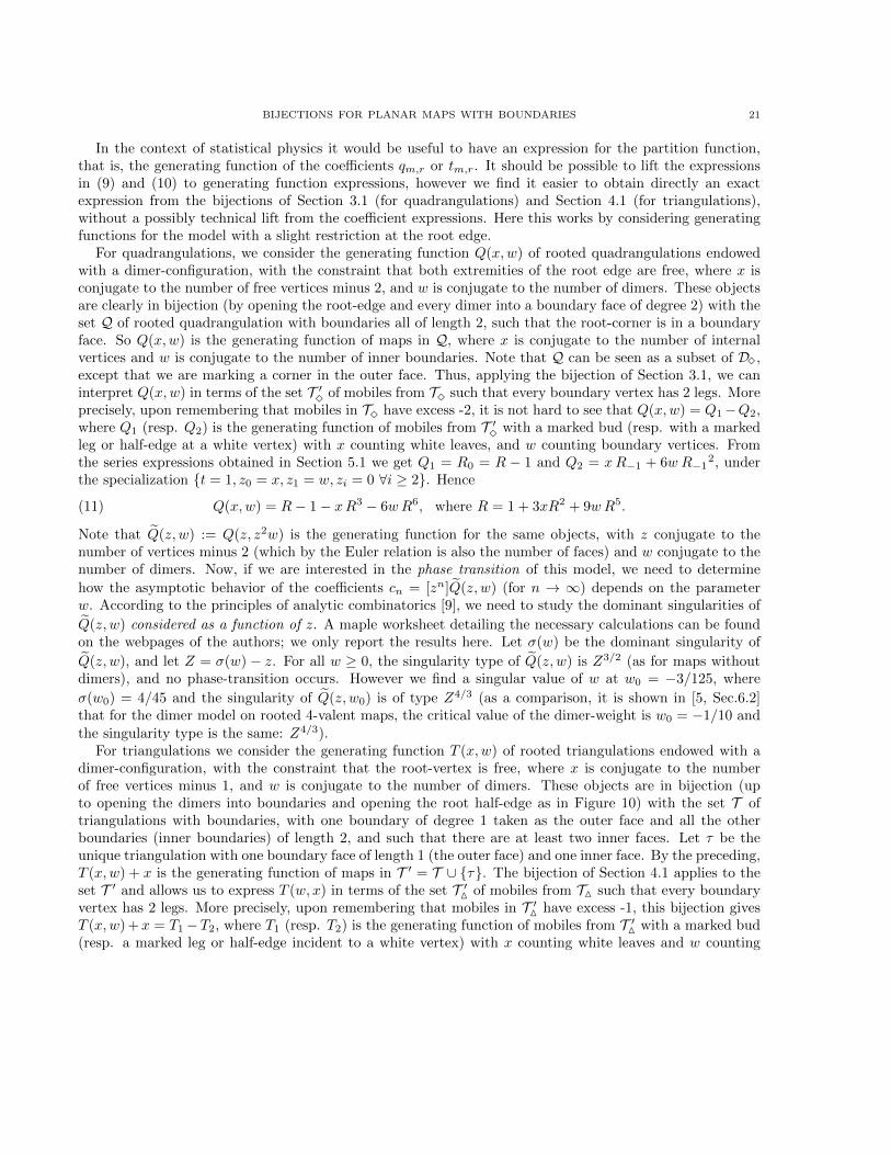
Figure 12. Left: a map in D3 endowed with its canonical orientation (all edges are 1-wayfor d = 3, the weight at the ingoing half-edge is indicated as the multiplicity of the arrow).Right: the corresponding mobile in T3 (all edges are black-white for d = 3, the weight atthe white extremity is indicated as the number of stripes across the edge).
• every boundary face f 6= fs has weight d+ deg(f), while the boundary of fs has weight 0.Note that the notion of 1-orientation for maps in DM given in Section 4 coincides with the notion of d/(d−2)-orientation for d = 1. Note also that if X is a 1-orientation of a map in D3 as defined in Section 3, thenmultiplying the weights of every internal half-edge of X by 2 gives a d/(d− 2)-orientation for d = 2.
Proposition 6.1. Let M be a map in Ed considered as a plane map by taking the outer face to be the markedboundary face fs. The map M has a d/(d − 2)-orientation if and only if M has fs-internal girth at least
d (i.e. is in Dd). Moreover, in this case, M has a unique d/(d − 2)-orientation in O−d. We call it thecanonical biorientation of M .
In the case where d is even, a map M ∈ Dd is bipartite if and only if all the internal half-edges of M haveeven weight in its canonical biorientation.
The proof is delayed to Section 7. Note that Proposition 6.1 includes Proposition 4.1 (case d = 1, withall internal faces of degree 3), and also Proposition 3.1 (case d = 2, with all internal faces of degree 4) upondividing all weights on internal half-edges by 2.
We denote by Td the set of mobiles corresponding to (canonically oriented) maps in Ed via the masterbijection. These are the boundary Z-mobiles satisfying the following properties (which readily imply thatthe weight of every half-edge is in −2,−1, . . . , d and the excess is −d):
• every edge has weight d− 2,• every black vertex has degree δ in d, d+ 1, d+ 2 and weight −δ + d,• every white vertex has weight d+ `, where ` is the number of incident legs.
Proposition 6.1 together with the master bijection (Theorem 2.2) then yield the following result.
Theorem 6.2. For each d ≥ 1, the set Dd of maps is in bijection with the set Td of Z-mobiles via the masterbijection. If a map M ∈ Dd corresponds to a mobile T ∈ Td by this bijection, then every internal face ofM corresponds to a black vertex of T of the same degree, every internal vertex of M corresponds to a whitevertex of T with no leg, and every boundary face f 6= fs in M corresponds to a white vertex of T havingdeg(f) legs.

24 O. BERNARDI AND E. FUSY
6.2. Bijections in internal girth d when at least one internal face has degree d. As a unificationand generalization of Sections 3.2 and 4.2, we treat here the case where the marked boundary face fs hasarbitrary degree, but at least one internal face has degree equal to the fs-internal girth.
For d, a ≥ 1, we denote by G(a)d the set of maps with boundaries, with a marked boundary face fs of degree
a, and a marked internal face fe of degree d, and where all internal faces have degree in d, d + 1, d + 2.Clearly, maps in G(a)
d have fs-internal girth at most d, and we denote by A(a)d the subset of maps from G(a)
d
having fs-internal girth d. For instance, A(a)M is the set of maps G(a)
1 = A(a)1 with all the internal faces of
degree 3. Similarly, A(2a)3 is the set of bipartite maps in G(2a)
2 with all the internal faces of degree 4; thebipartiteness condition is equivalent to the fact that every boundary has even length, and implies that the
fs-internal girth is 2 (hence A(2a)3 ⊂ A(2a)
2 ). Note that A(a)d is empty if a < d, and that A(d)
d identifies withthe set of maps from Dd with a marked internal face of degree d.
For M ∈ A(a)d we define a blocked region of M as an internally-enclosed set of faces S such that fs /∈ S
and fe ∈ S. Note that any blocked region has contour-length at least d, and that S = fe is a blockedregion of contour-length d. We also claim that if S1 and S2 are blocked regions of contour length d, thenS1 ∪ S2 is a blocked region of contour length d. Indeed, for any blocked regions S1, S2 the sets S1 ∪ S2 andS1 ∩ S2 are clearly blocked regions. Moreover, denoting `1, `2, `1∪2, and `1∩2 the contour lengths of S1, S2,S1 ∪ S2 and S1 ∩ S2 respectively, we have
`1 + `2 = `1∪2 + `1∩2 + 2∆,
where ∆ is the number of edges of M incident to a face in S1 \ S2 and a face in S2 \ S1. Therefore if`1 = `2 = d, then
`1∪2 ≤ `1 + `2 − `1∩2 ≤ d.Thus there is a blocked region S of contour length d containing all the other blocked regions of contourlength d. We call S the maximal blocked region of M .
A map M ∈ A(a)d is called reduced if S = fe is the unique blocked region of contour-length d. We denote
by B(a)d the subset of reduced maps from A(a)
d . We also denote by ~A(a)d (resp. ~B(a)
d ) the set of maps from
A(a)d (resp. from B(a)
d ) with a marked corner of fs. Note that B(a)d is empty for a < d and that B(d)
d consistsof exactly one map, with two faces of degree d, one internal and the other external.
As in Sections 3.2 and 4.2, we will consider a decomposition of maps in A(a)d into two parts, which, roughly
speaking, are obtained by cutting the map along the contour of the maximal blocked region. Let M be a
map in A(a)d . Let S be the maximal blocked region of M . Let E(S) be the set of edges of M having both
of their incident faces in S, and let V (S) be the set of vertices having all of their incident faces in S. It iseasy to see that the region H(S) := S ∪ E(S) ∪ V (S) is simply connected (homeomorphic to a disk). Wedenote by C(S) the cycle of M corresponding to the boundary of the region H(S). Hence the cycle C(S),which is not necessarily simple, is made of the edges incident to both a face in S and a face not in S. Wedenote by M1 the map obtained from M by keeping only the vertices in V (S), the edges in E(S), and thecycle C(S) turned into a simple cycle C ′(S) (so a single vertex on C(S) may correspond to several vertices ofC ′(S)). This process is illustrated in Figure 13. We denote by f ′s the marked boundary face (of degree d) of
M1 which lies outside of the cycle C ′(S). It is clear that M1 is in A(d)d . We denote by M2 the map obtained
from M by erasing all the vertices in V (S) and all the edges in E(S), so that the simply connected regionH(S) is replaced by a single marked internal face (of degree d) which we denote by f ′e. Note that the contour
C(S) of the marked face f ′e is not necessarily simple; see Figure 13. It is clear that M2 is in B(a)d . Hence
every map M in A(a)d decomposes into a pair (M1,M2) of maps in A(d)
d × B(a)d .

BIJECTIONS FOR PLANAR MAPS WITH BOUNDARIES 25
fs
SC ′(S)
fe
M1
M
M2
f ′s
fs
C(S)
f ′e
fe
Figure 13. The canonical decomposition of maps in A(a)d into a pair of maps in A(d)
d × B(a)d .
Conversely, given a pair (M1,M2) in A(d)d × B
(a)d , we can glue the contour of the marked boundary face
f ′s of M1 to the contour of the marked internal face of M2. Such a gluing produces a map in A(a)d such that
the maximal blocked region of M consists of all the faces of M1 distinct from its marked boundary face f ′s.There are d ways of gluing the two maps M1,M2 together, but one can easily make the gluing and ungluingcanonical at the level of maps with marked corners (formally, one needs to fix an arbitrary convention for
each map M2 ∈ ~B(a)d by choosing one of the corners of the marked internal face as the “gluing point” for
the marked corner of the maps in A(d)d ). We call this the canonical decomposition of the maps in A(a)
d . Wesummarize the above discussion:
Lemma 6.3. The canonical decomposition is a bijection between ~A(a)d and ~A(d)
d × ~B(a)d .
As mentioned earlier, the set of maps A(d)d identifies with the set of maps from Dd with a (secondary)
marked internal face of degree d. By Theorem 6.2, the set Dd of maps is in bijection with the set of Td ofmobile via the master bijection. Moreover, through the master bijection, marking an internal face of degreed in the map corresponds to marking a black vertex of degree d of the mobile. We denote Ud the set of
mobiles from Td with a marked black vertex of degree d. We also denote ~Ud the set of mobiles obtained frommobiles in Ud by marking one of the corners of the marked black vertex of degree d. The preceding remarkscan be summarized as follows:
Lemma 6.4. For all d ≥ 1, the set A(d)d (resp. ~A(d)
d ) of maps is in bijection with the set Ud (resp. ~Ud) ofZ-mobiles via the master bijection.
We will now characterize maps in B(a)d by canonical orientations, in order to get a bijection for these maps
as well. For a map M ∈ G(a)d , we define a d/(d − 2)-orientation of M as a consistent Z-biorientation of M
with weights in −2,−1, . . . , d such that:• every internal edge has weight d− 2,• every internal vertex has weight d,

26 O. BERNARDI AND E. FUSY
fe
fs
Figure 14. Left: a map in B(4)3 endowed with its canonical orientation (all edges are 1-way
for d = 3, the weight at the ingoing half-edge is indicated as the multiplicity of the arrow).
Right: the corresponding mobile in V(4)3 (the marked white vertex is represented as a square;
all edges are black-white for d = 3, the weight at the white extremity is indicated as thenumber of stripes across the edge).
• every internal face f has weight d− deg(f),• every boundary face f 6= fs has weight d+ deg(f), while fs has weight −d+ deg(fs).
Proposition 6.5. Let M be a map in G(a)d , let fs be its marked boundary face, and let fe be its marked
internal face. We consider M as a plane map by taking fe to be the outer face. The map M admits a
d/(d − 2)-orientation in Od if and only if M is in B(a)d (that is, M has fs-internal girth at least d, and is
reduced). In this case, the d/(d−2)-orientation in Od is unique. We call it the canonical biorientation of M .
Lastly, in the case where d and a are both even, a map M ∈ B(a)d is bipartite if and only if all the internal
half-edges of M have even weight in its canonical biorientation.
The proof is delayed to Section 7. Note that Proposition 6.5 includes Proposition 4.5 (case d = 1, withall internal faces of degree 3), and also Proposition 3.6 (case d = 2, with all internal faces of degree 4, andall boundary faces of even degree) upon dividing by 2 all weights on internal half-edges.
For a ≥ 1, we denote by V(a)d the set of mobiles corresponding to (canonically oriented) maps in B(a)
d via themaster bijection. By Theorem 2.2, these are the boundary Z-mobiles with a marked white vertex satisfyingthe following properties (which readily imply that the weight of every half-edge is in −2,−1, . . . , d and theexcess is d):
• every edge has weight d− 2,• every black vertex has degree δ in d, d+ 1, d+ 2 and weight −δ + d,• the marked white vertex has a incident legs and has weight a − d, while every non-marked white
vertex has weight d+ ` where ` is the number of incident legs.
We also denote by ~V(a)d the set of rooted mobiles obtained from mobiles in V(a)
d by marking one of the a legsof the marked white vertex.
Proposition 6.5 together with the master bijection (Theorem 2.2) and Lemmas 6.3 and 6.4 give thefollowing result (see Figure 14 for an example).
Theorem 6.6. For all d, a ≥ 1, the set B(a)d (resp. ~B(a)
d ) of maps is in bijection with the set V(a)d (resp.
~V(a)d ) of Z-mobiles via the master bijection. Moreover, for all d, a ≥ 1, the set ~A(a)
d of maps is in bijection
BIJECTIONS FOR PLANAR MAPS WITH BOUNDARIES 27
with the set ~Ud × ~V(a)d of pairs of Z-mobiles. The bijection is such that if the map M corresponds to the pair
of Z-mobiles (U, V ), then every non-marked internal face of M corresponds to a black vertex of U ∪V of thesame degree, every non-marked boundary face f of M corresponds to a non-marked white vertex of U ∪ Vhaving deg(f) legs, and every inner vertex of M corresponds to a white vertex of U ∪ V with no leg.
6.3. Expressions of the counting series. For d ≥ 1 we denote by Fd the set of maps from Dd with amarked corner in the marked boundary face. We denote by Fd ≡ Fd(xd, xd+1, xd+2; z0, z1, . . .) the associatedseries, with xδ (for δ ∈ d, d+ 1, d+ 2) conjugate to the number of internal faces of degree δ, z0 conjugateto the number of internal vertices, and zi (for i ≥ 1) conjugate to the number of non-marked boundary facesof degree i.
We will express Fd as the difference of two series of mobiles. First, observe that marking a corner in mapsfrom Dd, is equivalent to marking an ingoing outer half-edge in canonically oriented maps from Dd. Hence
Fd = K − L,
where K (resp. L) is the series for orientations from canonically oriented maps from Dd with a markedingoing half-edge (resp. with a marked ingoing inner half-edge).
Now we make the following observation about the master bijection Φ (which easily follows from the
definition of Φ):
Claim 6.7. For d ≥ 1, the master bijection Φ yields bijections (with same parameter correspondences)between:
• orientations from O−d with a marked ingoing half-edge and mobiles from B−d with a marked bud,
• orientations from O−d with a marked ingoing inner half-edge and mobiles from B−d with a markedhalf-edge (possibly a leg) incident to a white vertex.
By Theorem 6.2 and Claim 6.7, the series K (resp. L) is also the series of mobiles from Td with a markedbud (resp. with a marked half-edge incident to a white vertex), with xδ conjugate to the number of blackvertices of degree δ, and zi conjugate to the number of white vertices with i legs.
Similarly as in Sections 5.1 and 5.2, we introduce the notion of planted mobiles to formulate recursivedecompositions of mobiles. Precisely, for d ≥ 1, a planted mobile τ of type d is defined as a tree structurethat can be obtained as one of the two connected components after cutting a mobile T ∈ Td at the middleof an edge e (where e is a complete edge, not a bud nor a leg). The half-edge h of e belonging to the keptcomponent τ is called the root of τ , the incident vertex is the root-vertex of τ and the weight of h is theroot-weight of τ . For j ∈ −2, . . . , d we denote by Wj the set of planted mobiles of root-weight d − 2 − j,and we let Wj = Wj(xd, xd+1, xd+2; z0, z1, . . .) be the associated series, with as usual xδ conjugate to thenumber of black vertices of degree δ and zi conjugate to the number of white vertices with i legs. Note thatfor j ≥ d− 2 the root-vertex is black while for j < d− 2 the root-vertex is white. Similarly as in [3], we findfor j ∈ d− 2, d− 1, d,
Wj = [uj+2]
d+2∑i=d
xiui(1 +W0 + u−1W−1 + u−2
)i−1.
To treat the case of a white root-vertex we introduce the polynomials
h(k)j (X1, . . . , Xd) := [uj ]
(1−
d∑i=1
uiXi
)−k.
28 O. BERNARDI AND E. FUSY
For j ∈ −2, . . . , d− 3, the series Wj is then given by
Wj =∑k≥0
zk h(k+1)k+2+j(W1, . . . ,Wd).
Indeed, when the root-vertex w0 carries k legs, the total weight at w0 is k+ d, with a contribution d− 2− jfrom the root, and a total contribution k + 2 + j from the other incident half-edges at w0.
Then we can express K and L in terms of the Wj ’s. First, note that K = Wd−2 (indeed, a mobile fromTd with a marked bud identifies to a mobile in Wd−2, upon seeing the marked bud as a half-edge of weight0). We have
L =
d−3∑j=−2
WjWd−2−j +∑k≥1
zk h(k)d+k(W1, . . . ,Wd),
where the first sum gathers the cases where the marked half-edge belongs to an edge, and the second sumgathers the cases where the marked half-edge is a leg. Finally, we obtain:
Theorem 6.8. For d ≥ 1 the counting series Fd = Fd(xd, xd+1, xd+2; z0, z1, . . .) is given by
Fd = Wd−2 −d−3∑j=−2
WjWd−2−j −∑k≥1
zk h(k)d+k(W1, . . . ,Wd),
where the series W−2,W−1, . . . ,Wd are determined by the system
Wj =∑k≥0
zk h(k+1)k+2+j(W1, . . . ,Wd) for j ∈ −2, . . . , d− 3,
Wj = [uj+2]
d+2∑i=d
xiui(1 +W0 + u−1W−1 + u−2
)i−1for j ∈ d− 2, d− 1, d.
Note that Theorem 6.8 provides a generalization of the expression found in [2] for the series of rootedd-angulations of girth d, for d ≥ 3 (recovered here by taking xd+1 = xd+2 = 0 and zi = 0 for i ≥ 1).
We can also derive expressions for the generating functions of maps in ~A(a)d . More precisely, we deter-
mine below the generating function A(a)d = A
(a)d (xd, xd+1, xd+2; z0, z1, . . .) of ~A(a)
d , where the variable xδ isconjugate to the number of non-marked internal faces of degree δ, z0 is conjugate to the number of internalvertices, and for i ≥ 1 zi is conjugate to the number of non-marked boundaries of length i.
Let Ud ≡ Ud(xd, xd+1, xd+2; z0, z1, . . .) be the series of mobiles from ~Ud, with xδ conjugate to the numberof black vertices of degree δ, and zi conjugate to the number of white vertices with i legs. Since the mobiles
in ~Ud are obtained from the mobiles in Td by marking a corner at a black vertex of degree d, we get
Ud = (1 +W0)d.
For all a ≥ 1, let V(a)d ≡ V (a)
d (xd, xd+1, xd+2; z0, z1, . . .) be the generating function of mobiles in ~V(a)d with xδ
conjugate to the number of black vertices of degree δ, and zi conjugate to the number of non-marked whitevertices with i legs. The decomposition at the marked vertex gives
V(a)d = h
(a)a−d(W1, . . . ,Wd).
Since Theorem 6.6 yields A(a)d = Ud · V (a)
d we obtain the following result.
Theorem 6.9. For a, d ≥ 1 with a ≥ d, the series A(a)d = A
(a)d (xd, xd+1, xd+2; z0, z1, . . .) is given by
A(a)d = (1 +W0)d · h(a)
a−d(W1, . . . ,Wd),
with the same series Wi as in Theorem 6.8.

BIJECTIONS FOR PLANAR MAPS WITH BOUNDARIES 29
Theorem 6.9 provides a generalization of the expression found in [2] for the series of rooted d-angulationsof girth d (for d ≥ 3) with a boundary of length a (recovered here by taking xd+1 = xd+2 = 0 and zi = 0 fori ≥ 1).
For the case d = 2, let G(a)(t, x3, x4) be the series A(a)2 under the specialization x2 = 0, z0 = t, zi =
0 for i ≥ 1. This gives the enumeration of loopless maps with internal faces of degree either 3 or 4 (withrespective variables x3 and x4), a single boundary face of degree a, and a marked edge (indeed the markedinternal face of degree 2 can be seen as collapsed into a marked edge). By Theorem 6.9,
G(a)(t, x3, x4) = (1 +W0)2 · [ua−2](1− uW1 − u2W2)−a,
where the series W0,W1,W2 are given by the system
W−2 = t,
W−1 = tW1,
W0 = 2x3W−1(1 +W0) + 3x4W−2(1 +W0)2 + 3x4W−12(1 +W0),
W1 = x3(1 +W0)2 + 3x4W−1(1 +W0)2,
W2 = x4(1 +W0)3.
Under the further specialization x3 = 1, x4 = 0, the system simplifies to W2 = 0,W1 = (1+W0)2,W0 =2t(1 +W0)3, and we find
G(a)(t, 1, 0) = (1 +W0)2 · [ua−2](1− uW1)−a
= (1 +W0)2 ·(
2a− 3
a− 2
)W a−2
1 =
(2a− 3
a− 2
)(1 +W0)2a−2.
The Lagrange inversion formula then gives
[tn]G(a)(t, 1, 0) =
(2a− 3
a− 2
)1
n[yn−1](2a− 2)2n(1 + y)2a−3+3n
= 2n+1 (2a− 3)!
(a− 2)!2· (2a− 3 + 3n)!
n!(2a− 2 + 2n)!,
The coefficient [tn]G(a)(t, 1, 0) gives the number of loopless triangulations with one boundary of length a, ninternal vertices, a marked corner in the boundary face, and a marked edge. Since such a triangulation has2a+ 3n− 3 edges (by the Euler relation), we recover Mullin’s enumeration formula [12] whose first bijectiveproof was found in [13]:
Corollary 6.10 ([12, 13]). The number of loopless triangulations with one boundary of length a, n internal
vertices, and a marked corner in the boundary face is 2n+1 (2a− 3)!
(a− 2)!2· (2a− 4 + 3n)!
n!(2a− 2 + 2n)!.
Finally, similarly as in [2, 3], the expressions simplify slightly in the bipartite case. Let d = 2b with b ≥ 1.
Let F2b := F2b under the specialization x2b+1 = 0, z2i+1 = 0 for i ≥ 0. And let A(2a)2b := A
(2a)2b under the
same specialization. Using the fact that, in the bipartite case, the weights of internal half-edges are evenin the canonical orientations (and thus, so are the half-edge weights in the associated mobiles), we easilydeduce from Theorems 6.8 and 6.9 the following expressions:
30 O. BERNARDI AND E. FUSY
Corollary 6.11 (Bipartite case). The series F2b is expressed as
F2b = Vb−1 −b−2∑j=−1
VjVb−1−j −∑k≥1
z2kh(2k)b+k (V1, . . . , Vb),
where the series V−1, V0, . . . , Vb are determined by the system
Vj =∑k≥0
z2k h(2k+1)k+1+j (V1, . . . , Vb) for j ∈ −1, . . . , b− 2,
Vb−1 = x2b(1 + V0)2b−1 + (2b+ 1) x2b+2V−1(1 + V0)2b,
Vb = x2b+2(1 + V0)2b+1.
The series A(2a)2b is expressed as
A(2a)2b = (1 + V0)2b · h(2a)
a−b(V1, . . . , Vb).
We now gives analogues of Theorem 1.1 and Theorem 1.2 for other classes of triangulations and quad-rangulations. A map with boundaries having a marked boundary face fs is called internally loopless (resp.internally simple) if the fs-internal girth is at least 2 (resp. at least 3). We give below factorized countingformulas (analogous to Krikun’s formula (1.1)) when prescribing the number of internal vertices and thelengths of the boundaries for internally loopless and internally simple triangulations, and for internally sim-ple bipartite quadrangulations. This yields multivariate generalizations of the known formulas for the case ofa single boundary, which were originally due to Mullin for loopless triangulations [12] (as already recoveredin Corollary 6.10), and to Brown for simple triangulations [8] and simple quadrangulations [7].
Theorem 6.12. Let m ≥ 0, r ≥ 0, and let a, a1, . . . , ar be positive integers. For s ∈ 1, 2, 3 letTs[m; a, a1, . . . , ar] be the number of triangulations with m internal vertices, r + 1 (labeled from 0 to r)boundary faces f0, f1, . . . , fr such that deg(f0) = a, deg(fi) = ai for 1 ≤ i ≤ r, with a distinguished cornerin each boundary face, and such that the internal girth with respect to f0 is at least s. Note that Theorem 1.1gives a formula for |T1[m; a, a1, . . . , ar]|. Analogously, we get
|T2[m; a, a1, . . . , ar]| =(2a− 3)!
(a− 2)!2· 2m+r+1 · (3m+ 3r + 2b− 4)!
m!(2m+ 2r + 2b− 2)!
r∏i=1
ai
(2ai + 1
ai
),
|T3[m; a, a1, . . . , ar]| =2(2a− 3)!
(a− 3)!(a− 1)!· (4m+ 4r + 2b− 5)!
m!(3m+ 3r + 2b− 3)!
r∏i=1
ai
(2ai + 2
ai
),
where b = a+ a1 + . . .+ ar is the total boundary length.For s ∈ 1, 2 let Qs[m; a, a1, . . . , ar] be the number of quadrangulations with m internal vertices, r + 1
(labeled from 0 to r) boundary faces f0, f1, . . . , fr such that deg(f0) = 2a, deg(fi) = 2ai for 1 ≤ i ≤ r, witha distinguished corner in each boundary face, and such that the internal girth with respect to f0 is at least2s. Note that Theorem 1.2 gives a formula for |Q1[m; a, a1, . . . , ar]|. Analogously, we get
|Q2[m; a, a1, . . . , ar]| =3(3a− 2)!
(a− 2)!(2a− 1)!· (3m+ 3r + 3b− 4)!
m!(2m+ 2r + 3b− 2)!
r∏i=1
2ai
(3ai + 1
ai
),
where b = a+ a1 + . . .+ ar is the half total boundary length.
Proof. The proof is very similar to the proof of Theorem 1.1 and Theorem 1.2. It simply relies on the Lagrangeinversion formula starting from the generating function expressions given in Theorem 6.9 and Corollary 6.11.
BIJECTIONS FOR PLANAR MAPS WITH BOUNDARIES 31
We treat first the case of internally loopless triangulations. We consider the series A(a)2 =
(2a−3a−1
)(1+W0)2a−2,
where W0 is defined by W0 = 2∑k≥0 zk
(2k+1k
)(1 +W0)2k+3. Theorem 6.9 gives
|T2[m; a, a1, . . . , ar]| =1
e
(∏i≥1
inini!)· [zm0 zn1
1 . . . znh
h ]A(a)2 ,
where e = 3m+ 3r+ 2b− 3 corresponds to the number of edges, ni is the number of occurrences of i amonga1, . . . , ar, and h is the maximum of a1, . . . , ar. Then, the Lagrange inversion formula gives3
[zm0 zn11 . . . znh
h ]A(a)2 =
(2a− 2)!
(a− 2)!(a− 1)!2m+r · (3m+ 3r + 2b− 3)!
m!(2m+ 2r + 2b− 2)!·∏i≥1
1
ni!
(2i+ 1
i
)ni
,
which yields the formula for |T2[m; a, a1, . . . , ar]|.To treat the case of internally simple triangulations, we consider the series A
(a)3 =
(2a−4a−1
)(1 + W0)2a−3,
where W0 is given by W0 =∑k≥0 zk
(2k+2k
)(1 +W0)2k+4. Theorem 6.9 gives
|T3[m; a, a1, . . . , ar]| =1
f
(∏i≥1
inini!)· [zm0 zn1
1 . . . znh
h ]A(a)3 ,
where f = 2m+ 2r+ b− 2 corresponds to the number of internal faces, ni is the number of occurrences of iamong a1, . . . , ar, and h is the maximum of a1, . . . , ar. Then, the Lagrange inversion formula gives
[zm0 zn11 . . . znh
h ]A(a)3 =
(2a− 3)!
(a− 3)!(a− 1)!· (4m+ 4r + 2b− 4)!
m!(3m+ 3r + 2b− 3)!·∏i≥1
1
ni!
(2i+ 2
i
)ni
,
which yields the formula for |T3[m; a, a1, . . . , ar]|.Finally, for internally simple quadrangulations, we consider the series A
(2a)4 =
(3a−3a−2
)(1 + V0)3a−2, where
V0 is given by V0 =∑k≥0 z2k
(3k+1k
)(1 + V0)3k+3. Corollary 6.11 gives
|Q2[m; a, a1, . . . , ar]| =1
f
(∏i≥1
(2i)nini!)· [zm0 zn1
2 . . . znh
2h ]A(2a)4 ,
where f = m + r + b − 1 corresponds to the number of internal faces, ni is the number of occurrences of iamong a1, . . . , ar, and h is the maximum of a1, . . . , ar. Then, the Lagrange inversion formula gives
[zm0 zn12 . . . znh
2h ]A(2a)4 =
(3a− 2)!
(a− 2)!(2a− 1)!· (3m+ 3r + 3b− 3)!
m!(2m+ 2r + 3b− 2)!·∏i≥1
1
ni!
(3i+ 1
i
)ni
,
which yields the formula for |Q2[m; a, a1, . . . , ar]|.
7. Existence and uniqueness of the canonical orientations
In this section, we give the proof of Propositions 6.1 and 6.5 (which also imply Propositions 3.1, 3.6, 4.1,and 4.6).
3To apply the formula we let n = m+n1 + · · ·+nh and let y = tφ(y), with φ(y) = 2∑
k≥0 zk(2k+1
k
)(1 +y)2k+3. Then, with
ψ(y) = (1 + y)2a−2, we have [tn]ψ(y) = 1n
[yn−1]ψ′(y)φ(y)n, so that [zm0 zn11 . . . z
nhh ]ψ(y) = 1
n[yn−1]ψ′(y)[zm0 z
n11 . . . z
nhh ]φ(y)n.

32 O. BERNARDI AND E. FUSY
7.1. Preliminary results. We first set some notation and preliminary results about orientations. We callN-biorientation, a Z-biorientation with no negative weight (that is, the weight of every outgoing half-edge is0, and the weight of every ingoing half-edge is a positive integer).
Definition 7.1. Let M be a map with boundaries. Let V be the set of internal vertices, let E be the setof internal edges, and let B be the set of boundaries. Let α be a function from V ∪ B to N, and let β bea function from E to N. An α/β-orientation of M is a consistent N-biorientation, such that any vertex orboundary x ∈ V ∪B has weight α(x), and any edge e has weight β(e).
The following two lemmas are immediate consequences of the results in [2, Lemma 2 and Lemma 3] appliedto the map obtained from M by contracting each boundary into a single vertex.
Lemma 7.2. Let M,V,E,B, α, β be as in Definition 7.1. There exists a consistent α/β-orientation of Mif and only if
(i)∑x∈V ∪B α(x) =
∑e∈E β(e),
(ii) for each subset X ⊆ V ∪ B,∑x∈X α(x) ≥ ∑e∈EX
β(e), where EX ⊆ E is the subset of internaledges for which both endpoints are internal vertices in X or boundary vertices incident to a boundaryin X.
Moreover, α/β-orientations are accessible from an internal vertex v (resp. boundary vertex v) if and only if(iii) for each subset X ⊆ V ∪B not containing v (resp. not containing the boundary face incident to v),∑
v∈X α(x) >∑e∈EX
β(e).
Lemma 7.3. Let M be a plane map with boundaries, and let V,E,B, α, β be as in Definition 7.1. Supposethat there exists an α/β-orientation Ω of M . If the outer face of M is an internal face, then M admits aunique minimal α/β-orientation Ω0. If the outer face of M is a boundary face f satisfying α(f) = 0, thenM admits a unique almost-minimal α/β-orientation Ω0. In addition, in both cases, Ω is accessible from avertex v if and only if Ω0 is accessible from v.
Next, we state a parity lemma for orientations in Od.Lemma 7.4. Let O be a consistent Z-biorientation in Od (for some d ∈ Z\0), such that every internaledge, internal vertex, internal face, boundary, has even weight. Then every internal half-edge also has evenweight.
Proof. Let T be the boundary mobile associated with O by the master bijection (Theorem 2.2). The parityconditions of O imply that all edges and vertices of T have even weight. In particular an edge e of T eitherhas its two half-edges of odd weight, in which case e is called odd, or has its two half-edges of even weight,in which case e is called even. Let F be the subforest of T formed by the odd edges. Since every vertex ofT has even weight, it is incident to an even number of edges in F . Hence F has no leaf, so that F has noedge. Thus all edges of T are even, and by the local rules of the master bijection it implies that all internalhalf-edges of O have even weight. 7.2. Regular orientations. We now prove the existence of certain canonical orientations for bipartite mapsof internal girth 2b. This extends results proved in [2] to maps with boundaries.
Recall that a d-angulation with boundaries is a map such that every internal face has degree d. LetM be a bipartite 2b-angulation with boundaries, and let fs be a distinguished boundary face. We callb/(b− 1)-orientation of (M,fs) an α/β-orientation of M where,
• α(v) = b for every internal vertex, and β(e) = b− 1 for every internal edge,• α(f) = deg(f)/2 + b for every boundary face f 6= fs, and α(fs) = deg(fs)/2− b.
We say that a vertex x of M is d-blocked from the face fs if there is an internally-surrounded set of facesS containing all the faces incident to x but not fs, and having contour-length d.
BIJECTIONS FOR PLANAR MAPS WITH BOUNDARIES 33
Lemma 7.5. Let M be a bipartite 2b-angulation with boundaries, and let fs be a distinguished boundaryface. If M has fs-internal girth at least 2b, then there exists a b/(b − 1)-orientation of (M,fs). Moreover,any such orientation is accessible from the vertices incident to fs, and also from any vertex v which is not2b-blocked from fs.
Proof. We want to use Lemma 7.2. We start by checking Condition (i). Let V , E, and F be the sets ofinternal vertices, edges and faces respectively. Let V ′, E′ and B be the sets of boundary vertices, edges andfaces respectively. By definition,∑
x∈V ∪Bα(x)−
∑e∈E
β(e) = b|V |+ b(|B| − 2) +1
2
∑f∈B
deg(f)− (b− 1)|E|.
Moreover, the Euler formula gives |V |+ |F |+ |B| = 2+ |E| (because |V ′| = |E′|), while the incidence relationbetween faces and edges gives
∑f∈B deg(f) = |E′| and 2b|F | = 2|E| + |E′|. Using these identities gives∑
x∈V ∪Bα(x) −
∑e∈E
β(e) = 0 as wanted. We now check Condition (ii). Let X ⊆ V ∪ B, let VX = V ∩ X,
and let BX = B ∩ X. Let V ′X and E′X be the sets of vertices and edges incident to faces in BX (so thatEX ∪E′X are the edges of M with both endpoints in VX ∪ V ′X). Note that it is sufficient to check Condition(ii) for the subsets X such that the graph GX := (VX ∪ V ′X , EX ∪ E′X) is connected. Indeed, the quantity∑x∈X α(x) −∑e∈EX
β(e) is additive over the connected components of GX . So we now assume that GX
is connected and consider the corresponding submap MX of M . By definition,∑x∈X
α(x) −∑e∈EX
β(e) =
b|VX |+ b|BX | − 2b1fs∈X +|E′X |
2− (b− 1)|EX |, where 1fs∈X is 1 if fs ∈ X and 0 otherwise. Let FX be the
non-boundary faces of MX . The Euler formula reads |VX |+ |FX |+ |BX | = 2 + |EX |, so∑x∈X
α(x)−∑e∈EX
β(e) = 2b1fs /∈X +|E′X |
2+ |EX | − b|FX |.
Now, any face f ∈ FX corresponds to a set of faces S ⊆ F ∪ B of M which is internally-enclosed. Since Mhas fs-internal girth at least 2b, this implies that the faces in FX have degree at least 2b, except possiblyfor the face f ∈ FX containing fs (in the case fs /∈ X). Thus, the incidence relation gives 2b|FX | ≤2|EX |+ |E′X | − (2b− 1)1fs /∈X . Thus,∑
x∈Xα(x)−
∑e∈EX
β(e) ≥ 1fs /∈X .
This proves (ii) so there exists a b/(b − 1)-orientation of (M,fs). Moreover (iii) is also true for any vertexincident to fs, so that any b/(b− 1)-orientation is accessible from the vertices incident to fs.
Lastly, we consider a vertex v such that a b/(b− 1)-orientation Ω of (M,fs) is not accessible from v andwant to show that v is 2b-blocked from fs. Note that there is no directed path from v to fs in Ω (since Ω isaccessible from the vertices incident to fs). Let U be the set of vertices of M from which there is a directedpath toward fs, and let M ′ be the submap of M made of U and the edges with both endpoints in U . Thevertex v lies strictly inside a face f of M ′, and we consider the set S of faces of M corresponding to f .This is clearly an internally-enclosed set of faces of M (since boundary faces are directed cycles). Moreoverany edge of M strictly inside f , having one endpoint on f , is oriented away from this vertex, so that thetotal weight We of the edges strictly inside f is equal to the total weight Wv of the vertices strictly insidef . By combining the Euler relation and the incidence relation as above, the relation We = Wv becomesdeg(f) = 2b. Thus, the internally-enclosed set S has contour-length 2b. Hence, v is 2b-blocked from fs.

34 O. BERNARDI AND E. FUSY
For M a map with boundaries, we call star map of M , and denote M?, the map obtained from M byinserting a vertex vf , called star-vertex, in each internal face f , and joining vf by an edge to each corner off . The star map M? is considered as a map with boundaries (same boundaries as M). A star map is shownin Figure 15. The vertices and edges of M? which are in M are called M -vertices and M -edges, while theothers are called star-vertices and star-edges. If M is bipartite and fs is a distinguished boundary, we callb-regular orientation of (M?, fs) an α/β-orientation of M? where,
• α(v) = b for every internal M -vertex, and α(v) = deg(v)/2 + b for every star-vertex,• α(f) = deg(f)/2 + b for every boundary face f 6= fs, and α(fs) = deg(fs)/2− b,• β(e) = b− 1 for every internal M -edge, and β(e) = 1 for every star-edge.
M M?
Figure 15. A map with boundaries M , and the corresponding star map M? (with star-vertices colored black and M -vertices colored white).
Proposition 7.6. Let M be a bipartite map with boundaries, and let fs be a distinguished boundary face. IfM has fs-internal girth at least 2b, then there exists a b/(b− 1)-regular orientation of (M?, fs). Moreover,any such orientation is accessible from the vertices incident to fs, and also from any M -vertex v which isnot 2b-blocked from fs.
fQf Qf
Figure 16. Filling a face of M with a 2b-angulation without reducing the fs-internal girth(here b = 3): first insert a 2b-angulation Qf with one boundary f ′ of length deg(f) inside f(middle picture), and then connect each corner of f to a distinct corner of f ′ by a path oflength b− 1 (right picture).

BIJECTIONS FOR PLANAR MAPS WITH BOUNDARIES 35
Proof. We start by defining an orientation of M?, and we will show later that it has the desired properties.We first construct a 2b-angulation with boundaries N , by inserting a 2b-angulation in each internal face ofM in the manner illustrated in Figure 16. Precisely, for each internal face f 6= fs of M , we do the following:
• We insert a 2b-angulation Qf with one boundary f ′ of length deg(f). The 2b-angulation Qf is chosento have girth 2b, and Qf is placed so that f and f ′ are facing each other as in Figure 16.• We join by an edge each corner c of f to a distinct corner of f ′ by a path Pc of length b− 1 (without
creating edge crossings).It is easy to see that N has fs-internal girth 2b. Moreover, we can choose the maps Qf to be chordless (i.e.,no inner edge of Qf joins two vertices on the outer contour of Qf ). This easily ensures that any vertex ofM which is not 2b-blocked from fs in M is not 2b-blocked from fs in N (because no cycle of length at most2b using some edges of N \M can surround a vertex of M). Since N has fs-internal girth 2b, Lemma 7.6ensures the existence of a b/(b − 1)-orientation X of N . It is easy to see that, for each corner c of M , theweight wc of the half-edge of the path Pc incident to c is either 0 or 1 (otherwise the weight of the b − 2vertices on the path Pc cannot all be equal to b). We then define an orientation Y of M? by replacing eachquadrangulation Qf of N by a star-vertex vf , and replacing each path Pc by a single edge ec from the cornerc to vf with weight wc on the half-edge incident to c and 1 − wc on the half-edge incident to vf . We nowprove that Y is a b-regular orientation of (M?, fs). First, it is clear that the weight of every M -edge is b− 1,and the weight of every star-edge is 1. Second it is clear that the weight of every M -vertex is b, and forevery boundary face f the weight of the corresponding boundary is deg(f)/2 + b (same as in X). Thus itonly remains to check that the weight of each star-vertex vf is deg(f)/2 + b. Let Wf be the total weight,in X, of the half-edges incident to Qf on the paths Pc. It is easy to see that the weight of vf in Y is Wf
(because for any corner c the half-edge of Pc incident to Qf has weight 1−wc), hence we need to show thatWf = b+deg(f)/2. Let v and e be the number of vertices and edges of Qf . The Euler relation together withthe face-edge incidence relation imply that bv = (b− 1)e+ b+ deg(f)/2. In X the total weight of vertices inQf is bv and the total weight coming from edges in Qf is (b−1)e. Hence, Wf = bv− (b−1)e = b+deg(f)/2,as wanted. Thus, Y is a b-regular orientation of (M?, fs).
We know from Lemma 7.6 that the orientation X of N is accessible from the vertices incident to fs, andfrom any vertex which is not 2b-blocked from fs. Since the accessibility properties can only improve whencontracting X into Y , the orientation Y of M? is also accessible from the vertices incident to fs, and fromany vertex of M which is not 2b-blocked from fs.
7.3. Transfer lemma. Let N be a map and N? be the corresponding star map. We say that an N-orientation of N? is transferable if for any star-edge ε with an ingoing half-edge incident to an N -vertex v,the N -edge e following ε in clockwise order around v is oriented 1-way toward v. This property is illustratedin Figure 17(a).
Lemma 7.7. Let N be a plane map with boundaries having its outer face f0 of degree d, and let N? be thecorresponding star map. Let V be the set of internal N -vertices, let E be the set of internal N -edges, andlet B be the set of boundaries of N?. Let V ′ be the set of star-vertices, and let E′ be the set of star-edges ofN?. Let α : V ∪ V ′ ∪B → N, and let β : E ∪E′ → N, be functions such that there exists an α/β-orientationof N? which is accessible from the outer vertices of N .
In the case where the outer face f0 is a boundary face, we consider the star map N? as a plane map withouter face f0. Suppose that α(f0) = 0 and moreover the almost-minimal α/β-orientation of N? (which is
unique by Lemma 7.3) is transferable. In this case, there exists a unique Z-biorientation in O−d such that(i) any edge e ∈ E has weight β(e), and any vertex v ∈ V has weight α(v),
(ii) any boundary face f ∈ B has weight α(f), and any internal face f has weight α(vf )−∑
e∈E′ incident to vf
β(e).
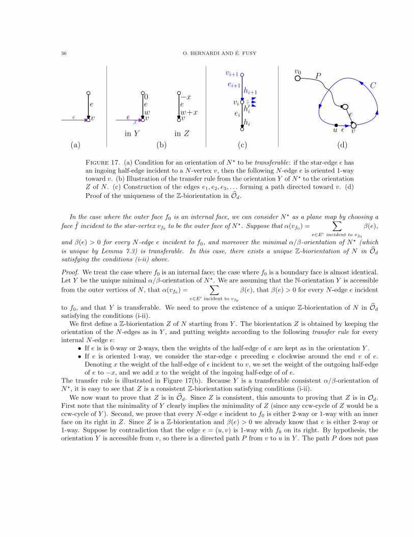
36 O. BERNARDI AND E. FUSY
vε
e
(a) (b)
v
e−xw+x
vε
e
x
0
wε
in Y in Z
e
v0
εu v
CP
(d)
ei
vi
hi
h′i
hi+1
ei+1
vi+1
(c)
Figure 17. (a) Condition for an orientation of N? to be transferable: if the star-edge ε hasan ingoing half-edge incident to a N -vertex v, then the following N -edge e is oriented 1-waytoward v. (b) Illustration of the transfer rule from the orientation Y of N? to the orientationZ of N . (c) Construction of the edges e1, e2, e3, . . . forming a path directed toward v. (d)
Proof of the uniqueness of the Z-biorientation in Od.
In the case where the outer face f0 is an internal face, we can consider N? as a plane map by choosing a
face f incident to the star-vertex vf0 to be the outer face of N?. Suppose that α(vf0) =∑
e∈E′ incident to vf0
β(e),
and β(e) > 0 for every N -edge e incident to f0, and moreover the minimal α/β-orientation of N? (which
is unique by Lemma 7.3) is transferable. In this case, there exists a unique Z-biorientation of N in Odsatisfying the conditions (i-ii) above.
Proof. We treat the case where f0 is an internal face; the case where f0 is a boundary face is almost identical.Let Y be the unique minimal α/β-orientation of N?. We are assuming that the N-orientation Y is accessible
from the outer vertices of N , that α(vf0) =∑
e∈E′ incident to vf0
β(e), that β(e) > 0 for every N -edge e incident
to f0, and that Y is transferable. We need to prove the existence of a unique Z-biorientation of N in Odsatisfying the conditions (i-ii).
We first define a Z-biorientation Z of N starting from Y . The biorientation Z is obtained by keeping theorientation of the N -edges as in Y , and putting weights according to the following transfer rule for everyinternal N -edge e:
• If e is is 0-way or 2-ways, then the weights of the half-edge of e are kept as in the orientation Y .• If e is oriented 1-way, we consider the star-edge ε preceding e clockwise around the end v of e.
Denoting x the weight of the half-edge of ε incident to v, we set the weight of the outgoing half-edgeof e to −x, and we add x to the weight of the ingoing half-edge of of e.
The transfer rule is illustrated in Figure 17(b). Because Y is a transferable consistent α/β-orientation ofN?, it is easy to see that Z is a consistent Z-biorientation satisfying conditions (i-ii).
We now want to prove that Z is in Od. Since Z is consistent, this amounts to proving that Z is in Od.First note that the minimality of Y clearly implies the minimality of Z (since any ccw-cycle of Z would be accw-cycle of Y ). Second, we prove that every N -edge e incident to f0 is either 2-way or 1-way with an innerface on its right in Z. Since Z is a Z-biorientation and β(e) > 0 we already know that e is either 2-way or1-way. Suppose by contradiction that the edge e = (u, v) is 1-way with f0 on its right. By hypothesis, theorientation Y is accessible from v, so there is a directed path P from v to u in Y . The path P does not pass
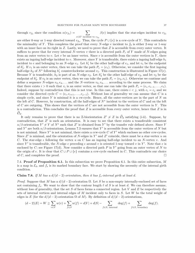
BIJECTIONS FOR PLANAR MAPS WITH BOUNDARIES 37
through vf0 since the condition α(vf0) =∑
e∈E′ incident to vf0
β(e) implies that the star-edges incident to vf0
are either 0-way or 1-way directed toward vf0 . Thus, the cycle P ∪ e is a ccw-cycle of Y . This contradictsthe minimality of Y . This completes the proof that every N -edge e incident to f0 is either 2-way or 1-waywith an inner face on its right in Z. Lastly, we need to prove that Z is accessible from every outer vertex. Itsuffices to prove that for every internal N -vertex v there is a directed path Pv of Y made of N -edges goingfrom an outer vertex to v. Let v be an inner vertex. Since v is accessible from the outer vertices in Y , thereexists an ingoing half-edge incident to v. Moreover, since Y is transferable, there exists a ingoing half-edge h1
incident to e and belonging to an N -edge e1. Let h′1 be the other half-edge of e1, and let v1 be the endpointof h′1. If v1 is an outer vertex, then we can take the path Pv = (e1). Otherwise, we consider the first ingoinghalf-edge h2 of N? following h′1 counterclockwise around v1. This construction is illustrated in Figure 17(c).Because Y is transferable, h2 is part of an N -edge e2. Let h′2 be the other half-edge of e2, and let v2 be theendpoint of h′2. If v2 is an outer vertex, then we can take the path Pv = (e2, e1). Otherwise we continue anddefine a sequence N -edges e3, e4, . . . and the N -vertices v3, v4, . . . according to the same process. We claimthat there exists i > 0 such that vi is an outer vertex, so that one can take the path Pv = (ei, ei−1, . . . , e1).Indeed, suppose by contradiction that this is not true. In this case, there exists i < j, with ei = ej and weconsider the directed cycle C = (ei, ei+1, . . . , ej−1). Without loss of generality we can assume that C is asimple cycle, and since Y is minimal it is a cw-cycle. Hence, all the outer-vertices are in the part of N onthe left of C. However, by construction, all the half-edges of N? incident to the vertices of C and on the leftof C are outgoing. This shows that the vertices of C are not accessible from the outer vertices in Y . Thisis a contradiction. This concludes the proof that Z is accessible from every outer vertex, hence that Z is in
Od.It only remains to prove that there is no Z-biorientation Z ′ 6= Z in Od satisfying (i-ii). Suppose, by
contradiction, that Z ′ is such an orientation. It is easy to see that there exists a transferable consistentα/β-orientation Y ′ 6= Y of N? such that Z ′ is obtained from Y ′ by the transfer rule defined above. Since Yand Y ′ are both α/β-orientations, Lemma 7.3 ensures that Y ′ is accessible from the outer vertices of N butis not minimal. Since Y ′ is not minimal, there exists a ccw-cycle C of Y ′ which encloses no other ccw-cycles.Since Z ′ is minimal, and the orientation of N -edges in Y ′ and Z ′ coincide, there must be a star-vertex u onC. The star-edge ε following the vertex u on C has an ingoing half-edge incident to an N -vertex v. Andsince Y ′ is transferable, the N -edge e preceding ε around v is oriented 1-way toward v in Y ′. Note that e isenclosed by C; see Figure 17(d). Now consider a directed path P in Y ′ going from an outer vertex of N tothe origin of e. It is clear that C ∪ P ∪ e contains a ccw-cycle enclosed in C. This contradicts our choiceof C, and completes the proof.
7.4. Proof of Proposition 6.1. In this subsection we prove Proposition 6.1. In this entire subsection, Mis a map in Ed, and fs is its marked boundary face. We start by showing the necessity of the internal girthcondition.
Claim 7.8. If M has a d/(d− 2)-orientation, then it has fs-internal girth at least d.
Proof. Suppose that M has a d/(d− 2)-orientation Ω. Let S be a non-empty internally-enclosed set of facesnot containing fs. We want to show that the contour length ` of S is at least d. We can therefore assume,without loss of generality, that the set S of faces forms a connected region. Let V and E be respectively thesets of internal vertices and internal edges of M incident only to faces in S. Let W be the total weight ofedges in E (for the d/(d− 2)-orientation Ω of M). By definition of d/(d− 2)-orientations,
(d− 2)|E| = W ≥∑v∈V
w(v) +∑f∈S
w(f) = d|V |+ d|S| −∑
f∈S, internal
deg(f) +∑
f∈S, boundary
deg(f).
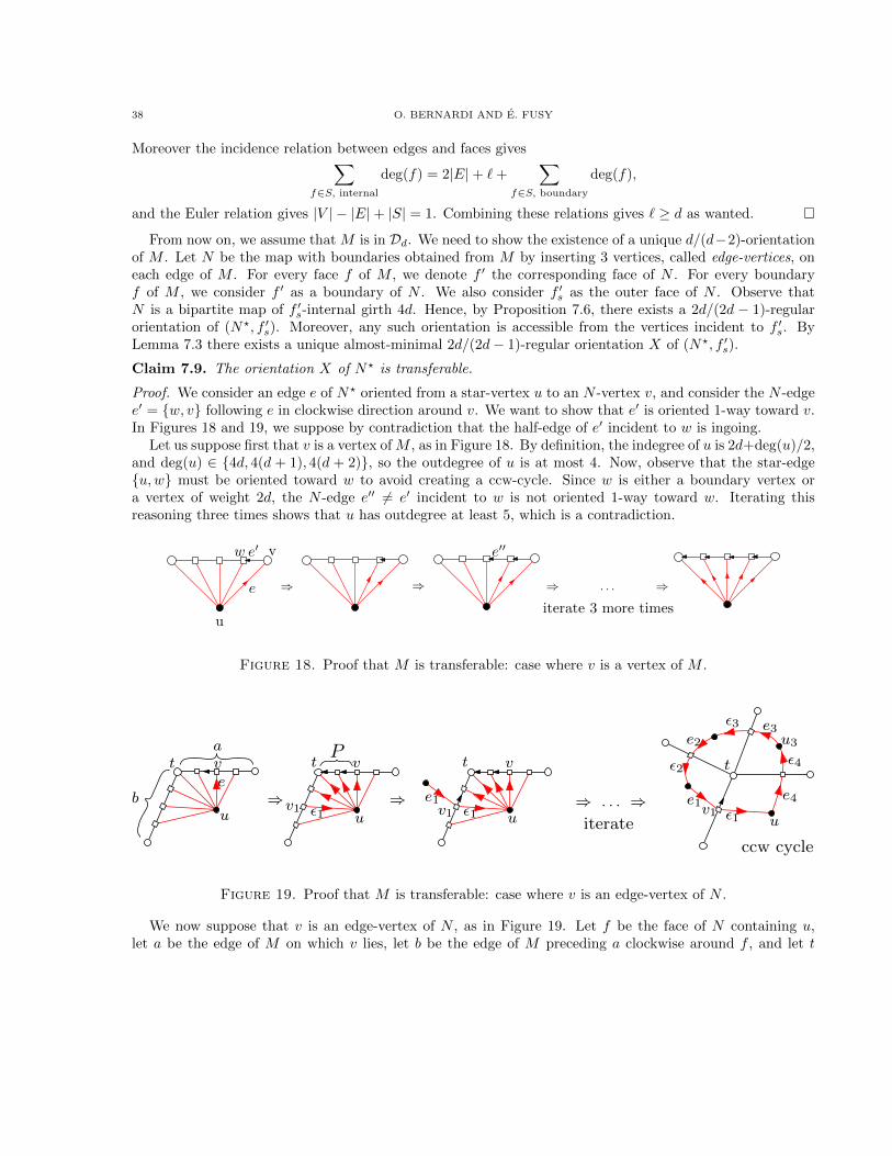
38 O. BERNARDI AND E. FUSY
Moreover the incidence relation between edges and faces gives∑f∈S, internal
deg(f) = 2|E|+ `+∑
f∈S, boundary
deg(f),
and the Euler relation gives |V | − |E|+ |S| = 1. Combining these relations gives ` ≥ d as wanted. From now on, we assume that M is in Dd. We need to show the existence of a unique d/(d−2)-orientation
of M . Let N be the map with boundaries obtained from M by inserting 3 vertices, called edge-vertices, oneach edge of M . For every face f of M , we denote f ′ the corresponding face of N . For every boundaryf of M , we consider f ′ as a boundary of N . We also consider f ′s as the outer face of N . Observe thatN is a bipartite map of f ′s-internal girth 4d. Hence, by Proposition 7.6, there exists a 2d/(2d − 1)-regularorientation of (N?, f ′s). Moreover, any such orientation is accessible from the vertices incident to f ′s. ByLemma 7.3 there exists a unique almost-minimal 2d/(2d− 1)-regular orientation X of (N?, f ′s).
Claim 7.9. The orientation X of N? is transferable.
Proof. We consider an edge e of N? oriented from a star-vertex u to an N -vertex v, and consider the N -edgee′ = w, v following e in clockwise direction around v. We want to show that e′ is oriented 1-way toward v.In Figures 18 and 19, we suppose by contradiction that the half-edge of e′ incident to w is ingoing.
Let us suppose first that v is a vertex of M , as in Figure 18. By definition, the indegree of u is 2d+deg(u)/2,and deg(u) ∈ 4d, 4(d + 1), 4(d + 2), so the outdegree of u is at most 4. Now, observe that the star-edgeu,w must be oriented toward w to avoid creating a ccw-cycle. Since w is either a boundary vertex ora vertex of weight 2d, the N -edge e′′ 6= e′ incident to w is not oriented 1-way toward w. Iterating thisreasoning three times shows that u has outdegree at least 5, which is a contradiction.
⇒ ⇒ ⇒ . . . ⇒iterate 3 more times
u
v
e
e′w e′′
Figure 18. Proof that M is transferable: case where v is a vertex of M .
⇒
ta
bu
⇒ . . . ⇒ε1 u
v
v1 ε1 u
v
v1⇒ e1
iterate
t t
ε1 u
e1
tε2
ε3
ε4
e2e3
e4
u3
ccw cycle
v
v1
e
P
Figure 19. Proof that M is transferable: case where v is an edge-vertex of N .
We now suppose that v is an edge-vertex of N , as in Figure 19. Let f be the face of N containing u,let a be the edge of M on which v lies, let b be the edge of M preceding a clockwise around f , and let t
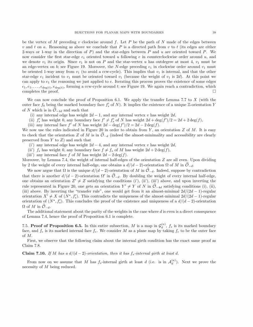
BIJECTIONS FOR PLANAR MAPS WITH BOUNDARIES 39
be the vertex of M preceding v clockwise around f . Let P be the path of N made of the edges betweenv and t on a. Reasoning as above we conclude that P is a directed path from v to t (its edges are either2-ways or 1-way in the direction of P ) and the star-edges between P and u are oriented toward P . Wenow consider the first star-edge ε1 oriented toward u following e in counterclockwise order around u, andwe denote v1 its origin. Since v1 is not on P and the star-vertex u has outdegree at most 4, v1 must bean edge-vertex on b; see Figure 19. Moreover, the N -edge preceding ε1 in clockwise order around v1 mustbe oriented 1-way away from v1 (to avoid a ccw-cycle). This implies that v1 is internal, and that the otherstar-edge e1 incident to v1 must be oriented toward v1 (because the weight of v1 is 2d). At this point wecan apply to e1 the reasoning we just applied to e. Iterating this process proves the existence of some edgesε1, e1, . . . , εdeg(t), edeg(t), forming a ccw-cycle around t; see Figure 19. We again reach a contradiction, whichcompletes the proof.
We can now conclude the proof of Proposition 6.1. We apply the transfer Lemma 7.7 to X (with theouter face f0 being the marked boundary face f ′s of N). It implies the existence of a unique Z-orientation Y
of N which is in O−4d and such that(i) any internal edge has weight 2d− 1, and any internal vertex v has weight 2d,
(ii) f ′s has weight 0, any boundary face f ′ 6= f ′s of N has weight 2d+ deg(f ′)/2 = 2d+ 2 deg(f),(iii) any internal face f ′ of N has weight 2d− deg(f ′)/2 = 2d− 2 deg(f).
We now use the rules indicated in Figure 20 in order to obtain from Y , an orientation Z of M . It is easy
to check that the orientation Z of M is in O−d (indeed the almost-minimality and accessibility are clearlypreserved from Y to Z) and such that
(i’) any internal edge has weight 2d− 4, and any internal vertex v has weight 2d,(ii’) fs has weight 0, any boundary face f 6= fs of M has weight 2d+ 2 deg(f),
(iii’) any internal face f of M has weight 2d− 2 deg(f).Moreover, by Lemma 7.4, the weight of internal half-edges of the orientation Z are all even. Upon dividing
by 2 the weight of every internal half-edge, one obtains a d/(d− 2)-orientation Ω of M in O−d.We now argue that Ω is the unique d/(d− 2)-orientation of M in O−d. Indeed, suppose by contradiction
that there is another d/(d − 2)-orientation Ω′ in O−d. By doubling the weight of every internal half-edge,one obtains an orientation Z ′ 6= Z satisfying the conditions (i’), (ii’), (iii’) above, and upon inverting the
rule represented in Figure 20, one gets an orientation Y ′ 6= Y of N in O−4d satisfying conditions (i), (ii),(iii) above. By inverting the “transfer rule”, one would get from it an almost-minimal 2d/(2d − 1)-regularorientation X ′ 6= X of (N?, f ′s). This contradicts the uniqueness of the almost-minimal 2d/(2d− 1)-regularorientation of (N?, f ′s). This concludes the proof of the existence and uniqueness of a d/(d− 2)-orientation
Ω of M in O−d.The additional statement about the parity of the weights in the case where d is even is a direct consequence
of Lemma 7.4, hence the proof of Proposition 6.1 is complete.
7.5. Proof of Proposition 6.5. In this entire subsection, M is a map in G(a)d , fs is its marked boundary
face, and fe is its marked internal face fe. We consider M as a plane map by taking fe to be the outer faceof M .
First, we observe that the following claim about the internal girth condition has the exact same proof asClaim 7.8.
Claim 7.10. If M has a d/(d− 2)-orientation, then it has fs-internal girth at least d.
From now on we assume that M has fs-internal girth at least d (i.e. is in A(a)d ). Next we prove the
necessity of M being reduced.

40 O. BERNARDI AND E. FUSY
Orientation Y of N :
internal edges w1 w2with w1 ≥ 0 and w2 ≥ 0
w1
w2=b−30
w2=b−2−1 b b′
w2=b−10
−1 b
−1 b
−1 b −1 b −1 b
−1
boundary edges 0 1 0 1 0 1 0 1
(a)
(b)
(c)
(d)
b′ b′′1 2
0 1
Orientation Z of M :Orientation Z of M :
w2
w2
−2 w2
−3 w2
0 1
Orientation Z of M :
w2=b−1 b −1 b −1 b(e)
−4 w2−1
Figure 20. Possible weights at a subdivided edge of M for the 2d/(2d − 1)-orientationY , and the associated orientation Z of M . We use the notation b = 2d, b′ = 2d − 1, andb′′ = 2d − 2. Case (a-e) correspond to internal edges. In (a) the weights w1, w2 of thehalf-edges incident to the vertices of M are both non-negative (in this case, w1 + w2 =4(b− 1)− 3b = 2d− 4 and the other weights are determined uniquely from w1, w2). In (b-e)we assume w1 = −1 and consider the possible sequences of weights.
Claim 7.11. If M has a d/(d− 2)-orientation in Od, then M is reduced.
Proof. Let M be a map in A(a)d admitting a d/(d− 2)-orientation Ω in Od. We denote by w(x) the weight of
a vertex or boundary x in Ω. Let S be a blocked region of contour length d. We need to show S = fe. LetV and E be respectively the set of inner vertices, and inner edges of M incident only to faces in S. Let U bethe set of vertices which are incident to both a face in S and a face not in S, and let H is the set of half-edgeswhich are part of an edge in E and whose incident vertex is in U . By definition of d/(d− 2)-orientations,
(d− 2)|E| ≥∑
h∈H,w(h)>0
w(h) +∑v∈V
w(v) +∑f∈S
w(f) = d|V |+d|F |−∑
f∈S, internal
deg(f) +∑
f∈S, boundary
deg(f).
Combining this relation with the incidence relation between faces and edges (∑
f∈S, internal
deg(f) = 2|E| +
d +∑
f∈S, boundary
deg(f)) and the Euler relation (|V | − |E| + |S| = 1) gives∑h∈H,w(h)>0 w(h) ≤ 0. Hence,
the weights of half-edges in H are non-positive. Equivalently no edge of E is oriented 1-way toward a vertexin U or oriented 2-way with a vertex in U . Moreover, since S is internally-enclosed, there cannot be anyboundary edge incident only to faces of S and oriented toward a vertex of U either. This implies that no
vertex of V can reach a vertex of U . Since Ω ∈ Od is accessible from the vertices incident to fe, it must be
that one of the vertices incident to fe is in U . Moreover, since Ω ∈ Od all the edges incident to fe are 2-waysor 1-way with an inner face on its right. This implies that the edges on the contour of S are incident to fe.Thus S = fe.
BIJECTIONS FOR PLANAR MAPS WITH BOUNDARIES 41
From now on we assume that M is reduced (i.e. is in B(a)d ). It remains to prove that M has a unique
d/(d − 2)-orientation in Od. The proof is similar to the proof of Proposition 6.1. Let N be the map withboundaries obtained from M by inserting 3 vertices, called edge-vertices, on each edge of M . For everyface f of M , we denote f ′ the corresponding face of N . For every boundary f of M , we consider f ′ asa boundary of N . We also consider f ′e as the outer face of N . Observe that N is a bipartite map of f ′s-internal girth at least 4d. Hence by Proposition 7.6 there exists a 2d/(2d− 1)-regular orientation of the starmap (N?, f ′s). By Lemma 7.3 there exists a unique minimal 2d/(2d − 1)-regular orientation X of (N?, f ′s).Moreover, since M is reduced, the vertices incident to f ′e are not 4d-blocked from fs. Thus (by the secondclaim of Proposition 7.6), X is accessible from the vertices incident to f ′e. We now want to apply the transferLemma 7.7 to X (with outer face the internal face f0 = f ′e). First, with the notation of Lemma 7.7, we haveβ(e) = 1 for every star-edge e and α(vf ′
e) = deg(f ′e)/2 + 2d = 4d =
∑e∈E′ incident to vf′
e
β(e). Moreover, X is
shown to be transferable by the same proof as for Claim 7.9. Thus we can apply Lemma 7.7, which implies
the existence of a unique Z-orientation Y of N which is in O4d and such that(i) any internal edge has weight 2d− 1, and any internal vertex v has weight 2d,
(ii) f ′s has weight 2a− 2d, any boundary face f ′ 6= f ′s of N has weight 2d+ deg(f ′)/2,(iii) any internal face f ′ of N has weight 2d− deg(f ′)/2.
We now use the rules indicated in Figure 20 in order to obtain from Y , an orientation Z of M . It is easy to
check that the orientation Z of M is in Od (indeed the minimality and accessibility are preserved from Y toZ) and such that
(i’) any internal edge has weight 2d− 4, and any internal vertex v has weight 2d,(ii’) fs has weight 2a− 2d, any boundary face f 6= fs of M has weight 2d+ 2 deg(f),
(iii’) any internal face f of M has weight 2d− 2 deg(f).Moreover, by Lemma 7.4, the weight of internal half-edges of the orientation Z are all even. Upon dividing
by 2 the weight of every internal half-edge, one obtains a d/(d− 2)-orientation Ω of M in Od.The uniqueness of the d/(d− 2)-orientation of M in Od is proved in the same way as for Proposition 6.1,
and the additional statement about the parity of the weight in the case where d, a are even follows fromLemma 7.4. This completes the proof of Proposition 6.5.
8. Concluding remarks
In this article we gave a bijective proof to all the known enumerative results for maps with boundaries(such as Krikun’s formula for triangulations with boundaries (1)), and also established new enumerativeresults (such as the formula for quadrangulations with boundaries (2)).
However, in view of the results established in [2, 3, 4], one could have hoped to obtain enumerative resultsfor slightly more general, or more natural, classes of maps with boundaries. Ideally one could hope toenumerate any class of maps with boundaries with control on the girth and on the degrees of both boundaryand internal faces. Alas, the girth parameter we are able to control through our bijections, the internal girthis a bit unnatural for maps with several boundaries (because it depends on a choice of a marked boundary).Second, for maps of internal girth d we could only allow internal faces degrees in d, d + 1, d + 2. Theselimitations were dictated by the proofs of our master bijection approach (existence of canonical orientations,and in particular Claim 7.9), and we do not think that further improvements are possible in this direction.
Looking at other approaches, we remark that one can count certain classes of maps with boundaries, witha control on a different girth parameter. Indeed, let us define the contractible girth of a plane map withboundaries, as the smallest length of a simple cycle enclosing a region with no boundary face (note thatgirth ≤ blocking girth ≤ contractible girth). It is not hard to see that using a generating function approach(by substitution) would allow one to compute the generating function of triangulations with boundaries of
42 O. BERNARDI AND E. FUSY
contractible girth d = 2 or 3 (starting from our results for d = 1), and the generating function of bipartitequadrangulations with boundaries, of contractible girth d = 4 (starting from our results for d = 2). But wedo not know if this method can be extended further, or if a direct bijective approach would work for theseclasses of maps. Still, there may be hope to obtain bijective results for other values of d for maps having atmost 2 boundaries (to be investigated. . . ).
Acknowledgments. The authors thank Jeremie Bouttier and Juanjo Rue for very interesting discussions.Olivier Bernardi was partially supported by NSF grant DMS-1400859. Eric Fusy was partly supported bythe ANR grant “Cartaplus” 12-JS02-001-01 and the ANR grant “EGOS” 12-JS02-002-01.
References
[1] M. Albenque and D. Poulalhon. Generic method for bijections between blossoming trees and planar maps. Electron. J.
Combin., 22(2):P2.38, 2015.
[2] O. Bernardi and E. Fusy. A bijection for triangulations, quadrangulations, pentagulations, etc. J. Combin. Theory Ser. A,
119(1):218–244, 2012.
[3] O. Bernardi and E. Fusy. Unified bijections for maps with prescribed degrees and girth. J. Combin. Theory Ser. A,
119(6):1352–1387, 2012.
[4] O. Bernardi and E. Fusy. Unified bijections for planar hypermaps with general cycle-length constraints. arXiv:1403.5371,2014.
[5] J. Bouttier, P. Di Francesco, and E. Guitter. Geodesic distance in planar graphs. Nucl. Phys., B663:535–567, 2003.
[6] J. Bouttier and E. Guitter. Distance statistics in quadrangulations with a boundary, or with a self-avoiding loop. Journalof Physics A: Mathematical and Theoretical, 42(46):465208, 2009.
[7] W. G. Brown. Enumeration of quadrangular dissections of the disk. Canad. J. Math., 17:302–317, 1965.
[8] W.G. Brown. Enumeration of triangulations of the disk. Proc. Lond. Math. Soc., pages 746–768, 1964.[9] P. Flajolet and R. Sedgewick. Analytic combinatorics. Cambridge University Press, 2009.
[10] M. Krikun. Explicit enumeration of triangulations with multiple boundaries. Electronic J. Combin., v14 R61, 2007.
[11] AM Mathai and PN Rathie. Enumeration of almost cubic maps. J. Combin. Theory Ser. B, 13(1):83–90, 1972.[12] R.C. Mullin. On counting rooted triangular maps. Canad. J. Math, 17(3):373–382, 1965.
[13] D. Poulalhon and G. Schaeffer. A bijection for triangulations of a polygon with interior points and multiple edges. Theoret.
Comput. Sci., 307(2):385–401, 2003.[14] D. Poulalhon and G. Schaeffer. Optimal coding and sampling of triangulations. Algorithmica, 46(3-4):505–527, 2006.
[15] R. P. Stanley. Enumerative combinatorics. Volume 2. Cambridge studies in advanced mathematics. Cambridge universitypress, Cambridge, New York, 1999.
[16] M. Staudacher. The Yang-Lee edge singularity on a dynamical planar random surface. Nuclear Physics B, 336(3):349–362,
1990.[17] W. T. Tutte. A census of slicings. Canad. J. Math., 14:708–722, 1962.


![Notes on the Catalan problem - scarpaz.com Mathematics... · Daniele Paolo Scarpazza Notes on the Catalan problem [1] An overview of Catalan problems • Catalan numbers appear as](https://static.fdocuments.us/doc/165x107/5b8526687f8b9ad34a8d9e0d/notes-on-the-catalan-problem-mathematics-daniele-paolo-scarpazza-notes.jpg)