Introduction - FrontPage - CompuCell3D · Web viewCompuCell3D Manual and Tutorial Version 3.6.2...
199
111Equation Chapter 1 Section 1CompuCell3D Manual and Tutorial Version 3.6.2 Maciej H. Swat, Julio Belmonte, Randy W. Heiland, Benjamin L. Zaitlen, James A. Glazier, Abbas Shirinifard Biocomplexity Institute and Department of Physics, Indiana University, 727 East 3 rd Street, Bloomington IN, 47405-7105, USA -1-
Transcript of Introduction - FrontPage - CompuCell3D · Web viewCompuCell3D Manual and Tutorial Version 3.6.2...
111Equation Chapter 1 Section 1CompuCell3D Manual and Tutorial
Version 3.6.2
Maciej H. Swat, Julio Belmonte, Randy W. Heiland, Benjamin L. Zaitlen, James A. Glazier, Abbas Shirinifard
Biocomplexity Institute and Department of Physics, Indiana University, 727 East 3rd Street, Bloomington IN, 47405-7105, USA
-1-
1 Introduction..................................................................................................................62 GGH Applications.......................................................................................................73 GGH Simulation Overview.........................................................................................7
3.1 Effective Energy...................................................................................................83.2 Dynamics............................................................................................................103.3 Algorithmic Implementation of Effective-Energy Calculations.........................11
4 CompuCell3D............................................................................................................135 Building CC3DML-Based Simulations Using CompuCell3D..................................15
5.1 Short Introduction to XML.................................................................................155.2 Cell-Sorting Simulation......................................................................................165.3 Angiogenesis Model...........................................................................................215.4 Bacterium-and-Macrophage Simulation.............................................................26
6 Python Scripting........................................................................................................326.1 A Short Introduction to Python...........................................................................336.2 General structure of CC3D Python scripts..........................................................346.3 Cell-Type-Oscillator Simulation.........................................................................366.4 Diffusing-Field-Based Cell-Growth Simulation.................................................416.5 Three-Dimensional Vascular Tumor Growth Model..........................................506.6 Subcellular Simulations Using BionetSolver......................................................59
7 Conclusion.................................................................................................................658 Acknowledgements....................................................................................................669 IX. XML Syntax of CompuCell3D modules.............................................................66
9.1.1 IX.1. Potts Section.......................................................................................669.1.1.1 IX.1.1 Lattice Type..............................................................................71
9.1.2 IX.2. Plugins Section...................................................................................739.1.2.1 IX.2.1. CellType Plugin.......................................................................739.1.2.2 IX.2.2. Simple Volume and Surface Constraints.................................739.1.2.3 IX.2.3.VolumeTracker and SurfaceTracker plugins............................749.1.2.4 IX.2.4. VolumeFlex Plugin..................................................................749.1.2.5 IX.2.5. SurfaceFlex Plugin...................................................................759.1.2.6 IX.2.6. VolumeLocalFlex Plugin.........................................................759.1.2.7 IX.2.7. SurfaceLocalFlex Plugin..........................................................769.1.2.8 IX.2.8. NeighborTracker Plugin...........................................................769.1.2.9 IX.2.9. Chemotaxis...............................................................................779.1.2.10 IX.2.10. ExternalPotential plugin.........................................................809.1.2.11 IX.2.11. CellOrientation Plugin...........................................................819.1.2.12 IX.2.12. PolarizationVector Plugin......................................................829.1.2.13 IX.2.13. CenterOfMass Plugin.............................................................839.1.2.14 IX.2.12. Contact Energy.......................................................................839.1.2.15 IX.2.13. ContactLocalProduct Plugin..................................................849.1.2.16 IX.2.14. AdhesionFlex Plugin..............................................................859.1.2.17 IX.2.15. ContactMultiCad Plugin.........................................................889.1.2.18 IX.2.15. MolecularContact...................................................................899.1.2.19 IX.2.15. ContactCompartment.............................................................899.1.2.20 IX.2.16. LengthConstraint Plugin........................................................90
-2-

9.1.2.21 IX.2.17. Connectivity Plugins..............................................................919.1.2.22 IX.2.18. Mitosis Plugin........................................................................939.1.2.23 IX.2.19. Secretion Plugin.....................................................................939.1.2.24 IX.2.20. PDESolverCaller Plugin.........................................................959.1.2.25 IX.2.21. Elasticity Plugin and ElasticityTracker Plugin......................969.1.2.26 IX.2.22. FocalPointPlasticity Plugin....................................................979.1.2.27 IX.2.23.Curvature Plugin...................................................................1019.1.2.28 IX.2.24.PlayerSettings Plugin............................................................1029.1.2.29 IX.2.25.BoundaryPixelTracker Plugin...............................................1039.1.2.30 IX.2.26. GlobalBoundaryPixelTracker..............................................1039.1.2.31 IX.2.27. PixelTracker Plugin..............................................................1049.1.2.32 IX.2.28. MomentOfInertia plugin......................................................1049.1.2.33 IX.2.29. SimpleClock plugin..............................................................1059.1.2.34 IX.2.30. ConvergentExtension plugin................................................105
9.1.3 IX.3. Steppable Section.............................................................................1059.1.3.1 IX.3.1 UniformInitializer Steppable...................................................1069.1.3.2 IX.3.2. BlobInitializer Steppable........................................................1079.1.3.3 IX.3.3. PIF Initializer.........................................................................1079.1.3.4 IX.3.4. PIFDumper Steppable............................................................1099.1.3.5 IX.3.5. Mitosis Steppabe....................................................................1099.1.3.6 IX.3.5. AdvectionDiffusionSolver.....................................................1119.1.3.7 IX.3.6. FlexibleDiffusionSolver.........................................................1149.1.3.8 IX.3.7. FastDiffusionSolver2D..........................................................1199.1.3.9 IX.3.8. KernelDiffusionSolver...........................................................1199.1.3.10 IX.3.9. ReactionDiffusionSolver........................................................1209.1.3.11 IX.3.10. Steady State diffusion solver................................................1229.1.3.12 IX.3.11. BoxWatcher Steppable.........................................................123
9.1.4 IX.4. Additional Plugins and Modules......................................................12410 X. References...........................................................................................................12411 Appendix..................................................................................................................131
11.1 1. Calculating Inertia Tensor in CompuCell3D.............................................13111.2 2.Calculating shape constraint of a cell – elongation term............................134
11.2.1 2.1. Diagonalizing inertia tensor................................................................13411.3 3 Forward Euler method for solving PDE's in CompuCell3D......................13511.4 4. Calculating center of mass when using periodic boundary conditions.....13611.5 5. Dividing cluster cells.................................................................................13711.6 7. Command line options of CompuCell3D..................................................139
11.6.1 7.1. CompuCell3D Player Command Line Options..................................13911.6.2 7.2. Runnig CompuCell3D in a GUI-Less Mode - Command Line Options.
14011.7 8. Managing CompuCell3D simulations (CC3D project files).....................14211.8 9. Keeping Track of Simulation Files (deprecated)......................................143
-3-
The goal of this manual is to teach biomodelers how to effectively use multi-scale, multi-cell simulation environment CompuCell3D to build, test, run and post-process simulations of biological phenomena occurring at single cell, tissue or even up to single organism levels. We first introduce basics of the Glazier-Graner-Hogeweg (GGH) model aka Cellular Potts Model (CPM) and then follow with essential information about how to use CompuCell3D and show simple examples of biological models implemented using CompuCell3D. Subsequently we will introduce more advanced simulation building techniques such as Python scripting and writing extension modules using C++. In everyday practice, however, the knowledge of C++ is not essential and C++ modules are usually developed by core CompuCell3D developers. However, to build sophisticated and biologically relevant models you will probably want to use Python scripting. Thus we strongly encourage readers to acquire at lease basic knowledge of Python. We don’t want to endorse any particular book but to guide users we might suggests names of the authors of the most popular books on Python programming: David Beazley, Mark Lutz, Mark Summerfield, Michael Dawson, Magnus Lie Hetland.
-4-
4 4 4 4 4 4
4 4 4 4 4 4
4 4 4 4 4 4
4 4 4 4 4 4
4 4 4 7 4 4
7 4 4 7 7 7
7 7 7 7 7 7
7 7 7 7 7 7
Detail of cell-lattice
1 IntroductionThe last decade has seen fairly realistic simulations of single cells that can confirm or predict experimental findings. Because they are computationally expensive, they can simulate at most several cells at once. Even more detailed subcellular simulations can replicate some of the processes taking place inside individual cells. E.g., Virtual Cell (http://www.nrcam.uchc.edu) supports microscopic simulations of intracellular dynamics to produce detailed replicas of individual cells, but can only simulate single cells or small cell clusters.
Simulations of tissues, organs and organisms present a somewhat different challenge: how to simplify and adapt single cell simulations to apply them efficiently to study, in-silico, ensembles of several million cells. To be useful, these simplified simulations should capture key cell-level behaviors, providing a phenomenological description of cell interactions without requiring prohibitively detailed molecular-level simulations of the internal state of each cell. While an understanding of cell biology, biochemistry, genetics, etc. is essential for building useful, predictive simulations, the hardest part of simulation building is identifying and quantitatively describing appropriate subsets of this knowledge. In the excitement of discovery, scientists often forget that modeling and simulation, by definition, require simplification of reality.
One choice is to ignore cells completely, e.g., Physiome (1) models tissues as continua with bulk mechanical properties and detailed molecular reaction networks, which is computationally efficient for describing dense tissues and non-cellular materials like bone, extracellular matrix (ECM), fluids, and diffusing chemicals (2, 3), but not for situations where cells reorganize or migrate.
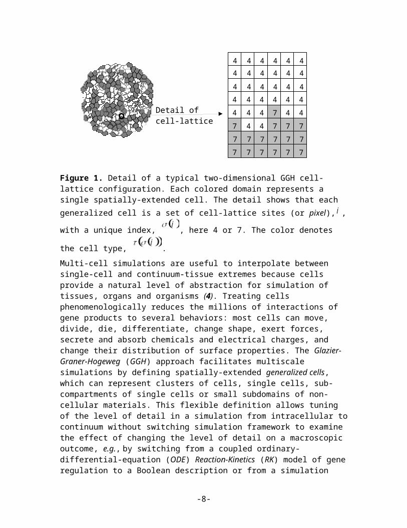
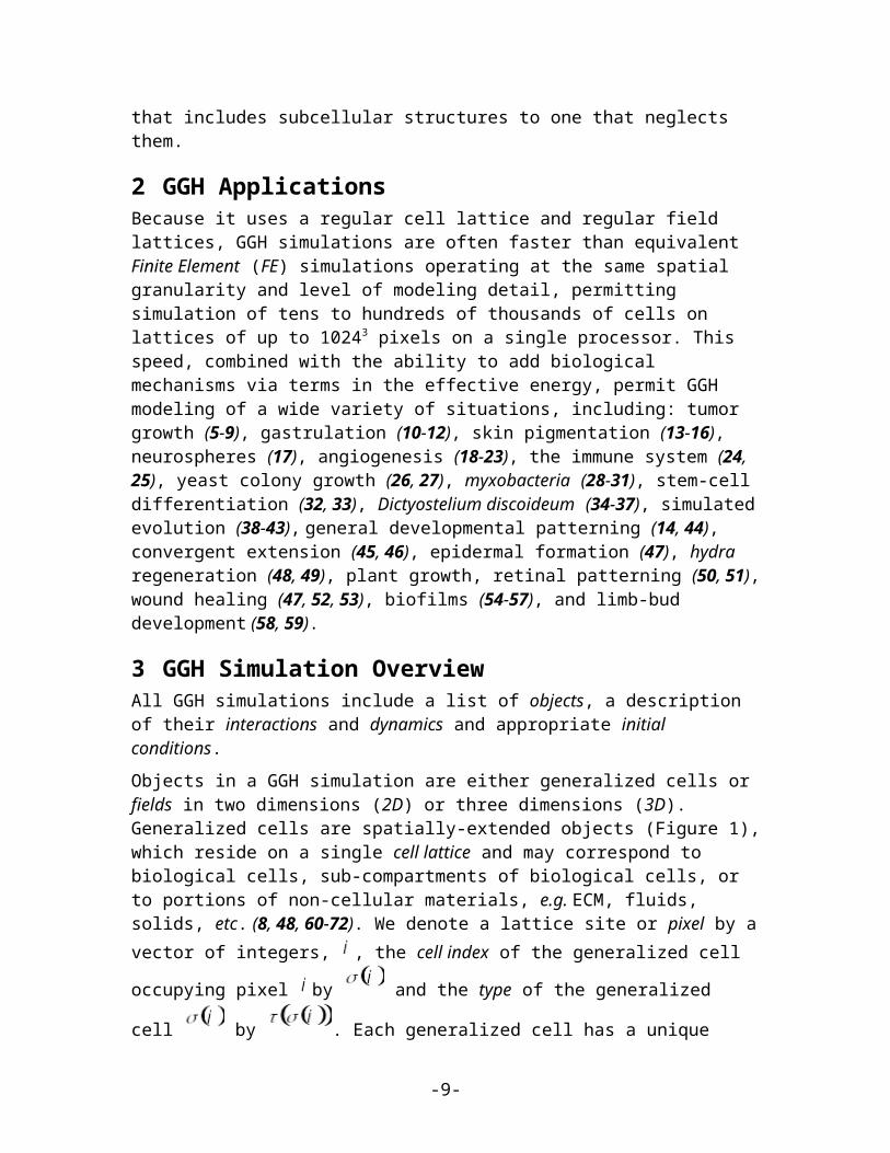
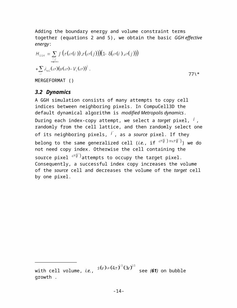
Figure 1. Detail of a typical two-dimensional GGH cell-lattice configuration. Each colored domain represents a single spatially-extended cell. The detail shows that each
generalized cell is a set of cell-lattice sites (or pixel), , with a unique index, , here
4 or 7. The color denotes the cell type, .
-5-

Multi-cell simulations are useful to interpolate between single-cell and continuum-tissue extremes because cells provide a natural level of abstraction for simulation of tissues, organs and organisms (4). Treating cells phenomenologically reduces the millions of interactions of gene products to several behaviors: most cells can move, divide, die, differentiate, change shape, exert forces, secrete and absorb chemicals and electrical charges, and change their distribution of surface properties. The Glazier-Graner-Hogeweg (GGH) approach facilitates multiscale simulations by defining spatially-extended generalized cells, which can represent clusters of cells, single cells, sub-compartments of single cells or small subdomains of non-cellular materials. This flexible definition allows tuning of the level of detail in a simulation from intracellular to continuum without switching simulation framework to examine the effect of changing the level of detail on a macroscopic outcome, e.g., by switching from a coupled ordinary-differential-equation (ODE) Reaction-Kinetics (RK) model of gene regulation to a Boolean description or from a simulation that includes subcellular structures to one that neglects them.
2 GGH ApplicationsBecause it uses a regular cell lattice and regular field lattices, GGH simulations are often faster than equivalent Finite Element (FE) simulations operating at the same spatial granularity and level of modeling detail, permitting simulation of tens to hundreds of thousands of cells on lattices of up to 10243 pixels on a single processor. This speed, combined with the ability to add biological mechanisms via terms in the effective energy, permit GGH modeling of a wide variety of situations, including: tumor growth (5-9), gastrulation (10-12), skin pigmentation (13-16), neurospheres (17), angiogenesis (18-23), the immune system (24, 25), yeast colony growth (26, 27), myxobacteria (28-31), stem-cell differentiation (32, 33), Dictyostelium discoideum (34-37), simulated evolution (38-43), general developmental patterning (14, 44), convergent extension (45, 46), epidermal formation (47), hydra regeneration (48, 49), plant growth, retinal patterning (50, 51), wound healing (47, 52, 53), biofilms (54-57), and limb-bud development (58, 59).
3 GGH Simulation Overview All GGH simulations include a list of objects, a description of their interactions and dynamics and appropriate initial conditions.
Objects in a GGH simulation are either generalized cells or fields in two dimensions (2D) or three dimensions (3D). Generalized cells are spatially-extended objects (Figure 1), which reside on a single cell lattice and may correspond to biological cells, sub-compartments of biological cells, or to portions of non-cellular materials, e.g. ECM, fluids, solids, etc. (8, 48, 60-72). We denote a lattice site or pixel by a vector of integers,
, the cell index of the generalized cell occupying pixel by and the type of the
generalized cell by . Each generalized cell has a unique cell index and contains many pixels. Many generalized cells may share the same cell type. Generalized cells permit coarsening or refinement of simulations, by increasing or decreasing the number of lattice sites per cell, grouping multiple cells into clusters or subdividing cells
-6-

into variable numbers of subcells (subcellular compartments). Compartmental simulation permits detailed representation of phenomena like cell shape and polarity, force transduction, intracellular membranes and organelles and cell-shape changes. For details on the use of subcells, which we do not discuss in this chapter see (27, 31, 73, 74). Each generalized cell has an associated list of attributes, e.g., cell type, surface area and volume, as well as more complex attributes describing a cell’s state, biochemical interaction networks, etc.. Fields are continuously-variable concentrations, each of which resides on its own lattice. Fields can represent chemical diffusants, non-diffusing ECM, etc.. Multiple fields can be combined to represent materials with textures, e.g., fibers.
Interaction descriptions and dynamics define how GGH objects behave both biologically and physically. Generalized-cell behaviors and interactions are embodied primarily in the effective energy, which determines a generalized cell’s shape, motility, adhesion and response to extracellular signals. The effective energy mixes true energies, such as cell-cell adhesion with terms that mimic energies, e.g., the response of a cell to a chemotactic gradient of a field (75). Adding constraints to the effective energy allows description of many other cell properties, including osmotic pressure, membrane area, etc. (76-83).
The cell lattice evolves through attempts by generalized cells to move their boundaries in a caricature of cytoskeletally-driven cell motility. These movements, called index-copy attempts, change the effective energy, and we accept or reject each attempt with a probability that depends on the resulting change of the effective energy, H, according to an acceptance function. Nonequilibrium statistical physics then shows that the cell lattice evolves to locally minimize the total effective energy. The classical GGH implements a modified version of a classical stochastic Monte-Carlo pattern-evolution dynamics, called Metropolis dynamics with Boltzmann acceptance (84, 85). A Monte Carlo Step (MCS) consists of one index-copy attempt for each pixel in the cell lattice.
Auxiliary equations describe cells’ absorption and secretion of chemical diffusants and extracellular materials (i.e., their interactions with fields), state changes within cells, mitosis, and cell death. These auxiliary equations can be complex, e.g., detailed RK descriptions of complex regulatory pathways. Usually, state changes affect generalized-cell behaviors by changing parameters in the terms in the effective energy (e.g., cell target volume or type or the surface density of particular cell-adhesion molecules).
Fields also evolve due to secretion, absorption, diffusion, reaction and decay according to partial differential equations (PDEs). While complex coupled-PDE models are possible, most simulations require only secretion, absorption, diffusion and decay, with all reactions described by ODEs running inside individual generalized cells. The movement of cells and variations in local diffusion constants (or diffusion tensors in anisotropic ECM) mean that diffusion occurs in an environment with moving boundary conditions and often with advection. These constraints rule out most sophisticated PDE solvers and have led to a general use of simple forward-Euler methods, which can tolerate them.
The initial condition specifies the initial configurations of the cell lattice, fields, a list of cells and their internal states related to auxiliary equations and any other information required to completely describe the simulation.
-7-
3.1 Effective EnergyThe core of GGH simulations is the effective energy, which describes cell behaviors and interactions.
One of the most important effective-energy terms describes cell adhesion. If cells did not stick to each other and to extracellular materials, complex life would not exist (86). Adhesion provides a mechanism for building complex structures, as well as for holding them together once they have formed. The many families of adhesion molecules (CAMs, cadherins, etc.) allow embryos to control the relative adhesivities of their various cell types to each other and to the noncellular ECM surrounding them, and thus to define complex architectures in terms of the cell configurations which minimize the adhesion energy.
To represent variations in energy due to adhesion between cells of different types, we define a boundary energy that depends on , the boundary energy per unit area between two cells ( ) of given types ( ) at a link (the interface between two neighboring pixels):
, 22\* MERGEFORMAT ()where the sum is over all neighboring pairs of lattice sites i and j (note that the neighbor range may be greater than one), and the boundary-energy coefficients are symmetric,
. 33\* MERGEFORMAT ()In addition to boundary energy, most simulations include multiple constraints on cell behavior. The use of constraints to describe behaviors comes from the physics of classical mechanics. In the GGH context we write constraint energies in a general elastic form:
. 44\* MERGEFORMAT ()
The constraint energy is zero if (the constraint is satisfied) and grows as value diverges from . The constraint is elastic because the exponent of 2 effectively creates an ideal spring pushing on the cells and driving them to satisfy the constraint. is the spring constant (a positive real number), which determines the constraint strength. Smaller values of allow the pattern to deviate more from the equilibrium condition (i.e., the condition satisfying the constraint). Because the constraint energy decreases smoothly to a minimum when the constraint is satisfied, the energy-minimizing dynamics used in the GGH automatically drives any configuration towards one that satisfies the constraint. However, because of the stochastic simulation method, the cell lattice need not satisfy the constraint exactly at any given time, resulting in
-8-
random fluctuations. In addition, multiple constraints may conflict, leading to configurations which only partially satisfy some constraints.
Because biological cells have a given volume at any time, most GGH simulations employ a volume constraint, which restricts volume variations of generalized cells from their target volumes:
, 55\* MERGEFORMAT ()
where for cell , denotes the inverse compressibility of the cell, is the
number of pixels in the cell (its volume), and is the cell’s target volume. This
constraint defines as the pressure inside the cell. A cell with
has a positive internal pressure, while a cell with has a negative internal pressure.
Since many cells have nearly fixed amounts of cell membrane, we often use a surface- area constraint of form:
, 66\* MERGEFORMAT ()
where is the surface area of cell s , is its target surface area, and is its inverse membrane compressibility.1
Adding the boundary energy and volume constraint terms together (equations 2 and 5), we obtain the basic GGH effective energy:
77\* MERGEFORMAT ()
3.2 DynamicsA GGH simulation consists of many attempts to copy cell indices between neighboring pixels. In CompuCell3D the default dynamical algorithm is modified Metropolis dynamics. During each index-copy attempt, we select a target pixel, , randomly from the cell lattice, and then randomly select one of its neighboring pixels, , as a source
1 Because of lattice discretization and the option of defining long range neighborhoods, the surface area of a cell scales in a non-Euclidian, lattice-dependent manner with cell
volume, i.e., see (61) on bubble growth .
-9-

Changedpixel
m/
0
: 0H kT
Hor
P e H
m/1 : 0H kTP e H
4 4 4 4 4 4
4 4 4 4 4 4
4 4 4 4 4 4
4 4 4 4 4 4
4 4 4 7 4 4
7 7 7 7 7 7
7 7 7 7 7 7
7 7 7 7 7 7
4 4 4 4 4 4
4 4 4 4 4 4
4 4 4 4 4 4
4 4 4 4 4 4
4 4 4 4 4 4
7 7 7 7 7 7
7 7 7 7 7 7
7 7 7 7 7 7
4 4 4 4 4 4
4 4 4 4 4 4
4 4 4 4 4 4
4 4 4 4 4 4
4 4 4 7 4 4
7 7 7 7 7 7
7 7 7 7 7 7
7 7 7 7 7 7
Index-copy succeeds
Index-copy fails
pixel. If they belong to the same generalized cell (i.e., if ) we do not need
copy index. Otherwise the cell containing the source pixel attempts to occupy the target pixel. Consequently, a successful index copy increases the volume of the source cell and decreases the volume of the target cell by one pixel.
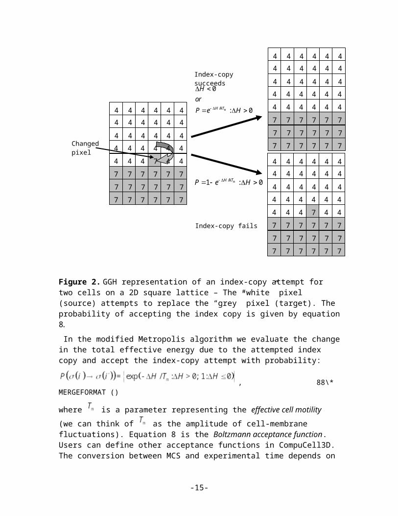
Figure 2. GGH representation of an index-copy attempt for two cells on a 2D square lattice – The “white” pixel (source) attempts to replace the “grey” pixel (target). The probability of accepting the index copy is given by equation 8.
In the modified Metropolis algorithm we evaluate the change in the total effective energy due to the attempted index copy and accept the index-copy attempt with probability:
, 88\* MERGEFORMAT ()
where is a parameter representing the effective cell motility (we can think of as the amplitude of cell-membrane fluctuations). Equation 8 is the Boltzmann acceptance function. Users can define other acceptance functions in CompuCell3D. The conversion
between MCS and experimental time depends on the average values of . MCS and experimental time are proportional in biologically-meaningful situations (87-90).
-10-

3.3 Algorithmic Implementation of Effective-Energy Calculations
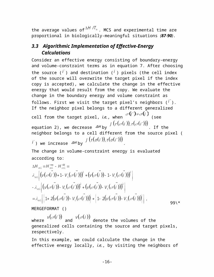
Consider an effective energy consisting of boundary-energy and volume-constraint terms as in equation 7. After choosing the source ( ) and destination ( ) pixels (the cell index of the source will overwrite the target pixel if the index copy is accepted), we calculate the change in the effective energy that would result from the copy. We evaluate the change in the boundary energy and volume constraint as follows. First we visit the target pixel’s neighbors ( ). If the neighbor pixel belongs to a different generalized cell from
the target pixel, i.e., when (see equation 2), we decrease ΔH by
. If the neighbor belongs to a cell different from the source pixel (
) we increase ΔH by .
The change in volume-constraint energy is evaluated according to:
99\* MERGEFORMAT ()
where and denote the volumes of the generalized cells containing the source and target pixels, respectively.
In this example, we could calculate the change in the effective energy locally, i.e., by visiting the neighbors of the target of the index copy. Most effective energies are quasi-local, allowing calculations of similar to those presented above. The locality of the effective energy is crucial to the utility of the GGH approach. If we had to calculate the effective energy for the entire cell lattice for each index-copy attempt, the algorithm would be prohibitively slow.
-11-
Target pixel
Pixels contributing to the boundary energy
Source pixel
1v i
1v i
v i
v i
8 white,greyJ
8 white,greyJ
6 white,greyJ
6 white,greyJ
1
1
1
1
2
22
2
3
3
3
3
4
4
4
4 4
4
4
4 11
11
1
1
2 2
2
22
2
3
3
3
3
3
3
4
4
444
4
4
4
44 4
4
Figure 3. Calculating changes in the boundary energy and the volume-constraint energy on a nearest-neighbor square lattice.
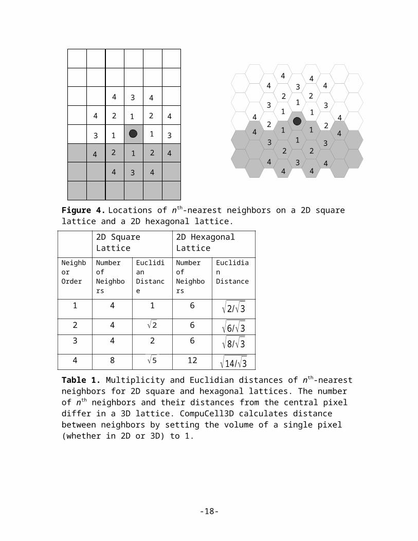
For longer-range interactions we use the appropriate list of neighbors, as shown in Figure4 and Table 1. Longer-range interactions are less anisotropic but result in slower simulations.
Figure 4. Locations of nth-nearest neighbors on a 2D square lattice and a 2D hexagonal lattice.
2D Square Lattice 2D Hexagonal Lattice
-12-
Neighbor Order
Number of Neighbors
Euclidian Distance
Number of Neighbors
Euclidian Distance
1 4 1 6 √2/√32 4 √2 6 √6/√33 4 2 6 √8/√34 8 √5 12 √14 /√3
Table 1. Multiplicity and Euclidian distances of nth-nearest neighbors for 2D square and hexagonal lattices. The number of nth neighbors and their distances from the central pixel differ in a 3D lattice. CompuCell3D calculates distance between neighbors by setting the volume of a single pixel (whether in 2D or 3D) to 1.
4 CompuCell3DCompuCell3D allows users to build sophisticated models more easily and quickly than does specialized custom code. It also facilitates model reuse and sharing.A CC3D model consists of CC3DML scripts (an XML-based format), Python scripts, and files specifying the initial configurations of any fields and the cell lattice. The CC3DML script specifies basic GGH parameters such as lattice dimensions, cell types, biological
mechanisms and auxiliary information such as file paths. Python scripts primarily monitor the state of the simulation and implement changes in cell behaviors, e.g. changing the type of a cell depending on the oxygen partial pressure in a simulated tumor.CompuCell3D is modular, loading only the modules needed for a particular model. Modules which calculate effective energy terms or monitor events on the cell lattice are called plugins. Effective-energy calculations are invoked every pixel copy attempt, while cell-lattice monitoring plugins run whenever an index copy occurs. Because plugins are the most frequently called modules in CC3D, most are coded in C++ for speed.Modules called steppables usually performs operations on cells, not on pixels. Steppables are called at fixed intervals measured in Monte-Carlo steps. Steppables have three main
-13-
Figure 5 Flow chart of the GGH algorithm as implemented in CompuCell3D.
uses: 1) to adjust cell parameters in response to simulation events2, 2) to solve PDEs, 3) to load simulation initial conditions or save simulation results. Most steppables are implemented in Python. Much of the flexibility of CC3D comes from user-defined Python steppables. The CC3D kernel supports parallel computation in shared-memory architectures (via OpenMP), providing substantial speedups on multi-core computers. Besides the computational kernel of CC3D, the main components of the CC3D environment are: 1) Twedit++-CC3D – a model editor and code generator, 2) CellDraw – a graphical tool for configuring the initial cell lattice, 3) CC3D Player – a graphical tool for running, replaying and analyzing simulations.Twedit++-CC3D provides a Simulation Wizard which generates draft CC3D model code based on high-level specification of simulation objects such as cell types and their behaviors, fields and interactions. Currently, the user must adjust default parameters in the auto-generated draft code, but later versions will provide interfaces for parameter specification. Twedit++-CC3D also provides a Python code-snippet generator, which simplifies coding Python CC3D modules.
CellDraw allows users to draw regions which it fills with cells of user-specified types. It also imports microscope images for manual segmentation.CC3D Player is a graphical interface which loads and executes CC3D models. It allows users to change model parameters during execution (steering), define multiple 2D and 3D visualizations of the cell lattice and fields and conduct real-time simulation analysis. CC3D Player also supports batch mode execution on clusters.
Figure 6 CellDraw graphics tools and GUI.
2 We will use the word model to describe the specification of a particular biological system and simulation to refer to a specific instance of the execution of such a model.
-14-
5 Building CC3DML-Based Simulations Using CompuCell3D
To show how to build simulations in CompuCell3D, the reminder of this chapter provides a series of examples of gradually increasing complexity. For each example we provide a brief explanation of the physical and/or biological background of the simulation and listings of the CC3DML configuration file and Python scripts, followed by a detailed explanation of their syntax and algorithms. We begin with three examples using only CC3DML to define simulations.
We use Twedit++-CC3D code generation and explain how to turn automatically-generated draft code into executable models. All of the parameters appearing in the autogenerated simulation scripts are set to their default values.
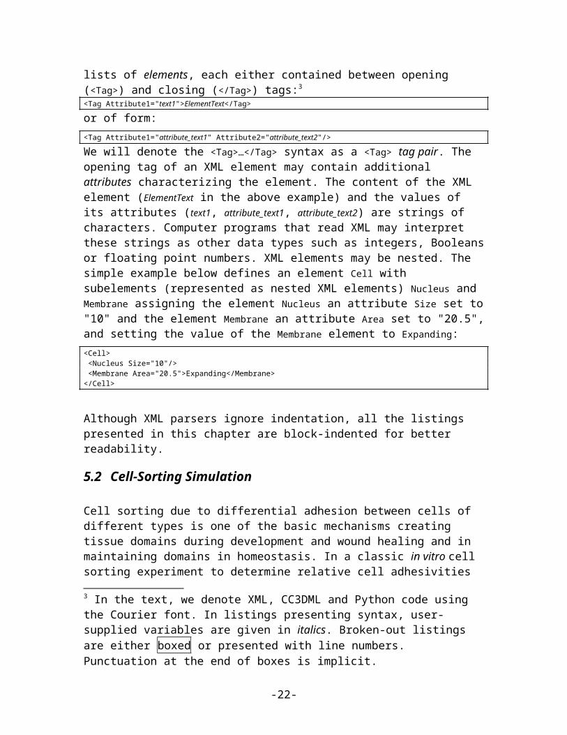
5.1 Short Introduction to XMLXML is a text-based data-description language, which allows standardized representations of data. XML syntax consists of lists of elements, each either contained between opening (<Tag>) and closing (</Tag>) tags:3
<Tag Attribute1="text1">ElementText</Tag>
or of form:<Tag Attribute1="attribute_text1" Attribute2="attribute_text2"/>
We will denote the <Tag>…</Tag> syntax as a <Tag> tag pair. The opening tag of an XML element may contain additional attributes characterizing the element. The content of the XML element (ElementText in the above example) and the values of its attributes (text1, attribute_text1, attribute_text2) are strings of characters. Computer programs that read XML may interpret these strings as other data types such as integers, Booleans or floating point numbers. XML elements may be nested. The simple example below defines an element Cell with subelements (represented as nested XML elements) Nucleus and Membrane assigning the element Nucleus an attribute Size set to "10" and the element Membrane an attribute Area set to "20.5", and setting the value of the Membrane element to Expanding:<Cell> <Nucleus Size="10"/> <Membrane Area="20.5">Expanding</Membrane></Cell>
Although XML parsers ignore indentation, all the listings presented in this chapter are block-indented for better readability.
5.2 Cell-Sorting Simulation
Cell sorting due to differential adhesion between cells of different types is one of the
3 In the text, we denote XML, CC3DML and Python code using the Courier font. In listings presenting syntax, user-supplied variables are given in italics. Broken-out listings are either boxed or presented with line numbers. Punctuation at the end of boxes is implicit.
-15-
basic mechanisms creating tissue domains during development and wound healing and in maintaining domains in homeostasis. In a classic in vitro cell sorting experiment to determine relative cell adhesivities in embryonic tissues, mesenchymal cells of different types are dissociated, then randomly mixed and reaggregated. Their motility and differential adhesivities then lead them to rearrange to reestablish coherent homogenous domains with the most cohesive cell type surrounded by the less. The simulation of the sorting of two cell types was the original motivation for the development of GGH methods. Such simple simulations show that the final configuration depends only on the hierarchy of adhesivities, while the sorting dynamics depends on the ratio of the adhesive energies to the amplitude of cell fluctuations.
To invoke the simulation wizard to create a simulation, we click CC3DProject->New CC3D Project in the menu bar. In the initial screen we specify the name of the model (cellsorting), its storage directory (C:\CC3DProjects) and whether we will store the model as pure CC3DML, Python and CC3DML or pure Python. This tutorial will use Python and CC3DML.
Figure 7 Invoking the CompuCell3D Simulation Wizard from Twedit++.
On the next page of the Wizard we specify GGH global parameters, including cell-lattice dimensions, the cell fluctuation amplitude, the duration of the simulation in Monte-Carlo steps and the initial cell-lattice configuration.In this example, we specify a 100x100x1 cell-lattice, i.e., a 2D model, a fluctuation amplitude of 10, a simulation duration of 10000 MCS and a pixel-copy range of 2. BlobInitializer initializes the simulation with a disk of cells of specified size.
-16-
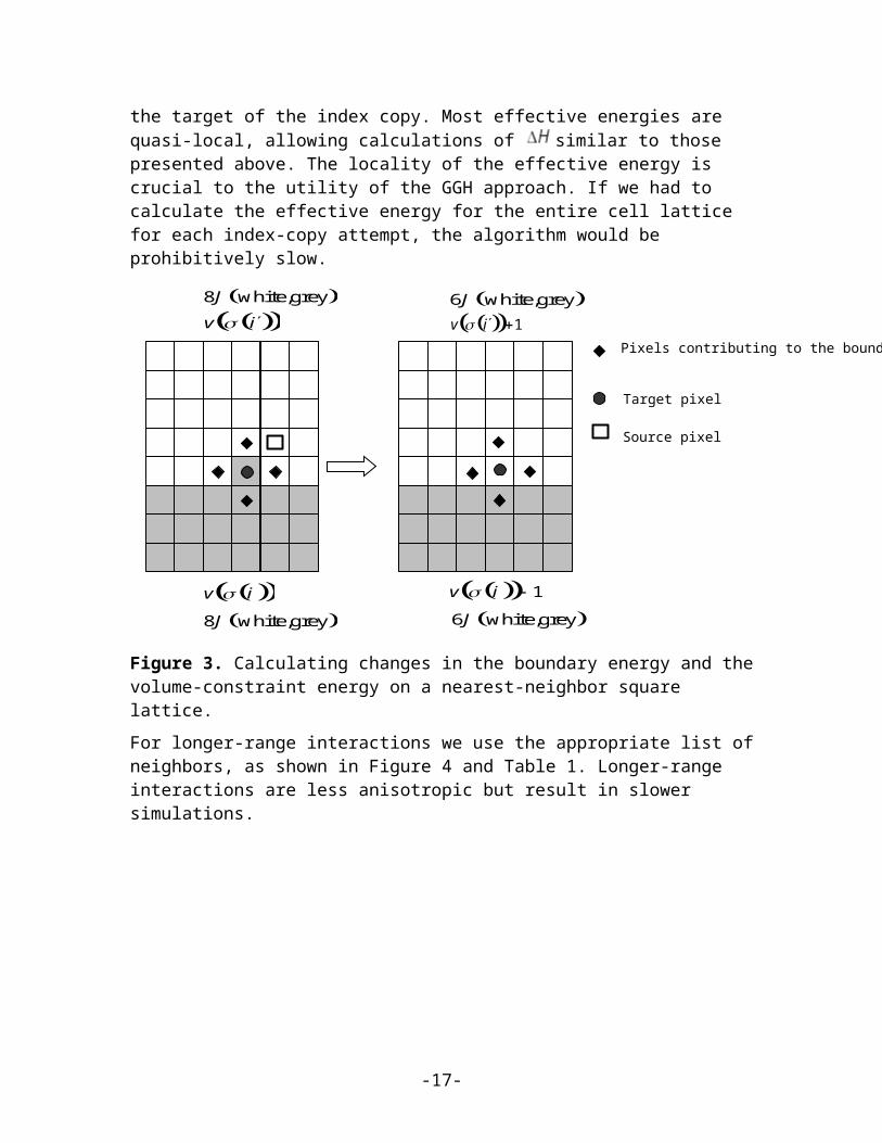
Figure 8 Specification of basic cell-sorting properties in Simulation Wizard.
On the next Wizard page we name the cell types in the model. We will use two cells types: Condensing (more cohesive) and NonCondensing (less cohesive). CC3D by default includes a special generalized-cell type Medium with unconstrained volume which fills otherwise unspecified space in the cell-lattice.
Figure 9 Specification of cell-sorting cell types in Simulation Wizard.
We skip the Chemical Field page of the Wizard and move to the Cell Behaviors and Properties page. Here we select the biological behaviors we will include in our model. Objects in CC3D have no properties or behaviors unless we specify then explicitly. Since cell sorting depends on differential adhesion between cells, we select the Contact Adhesion module from the Adhesion section and give the cells a defined volume using the Volume Constraint module.
Figure 10 Selection of cell-sorting cell behaviors in Simulation Wizard.4
We skip the next page related to Python scripting, after which Twedit++-CC3D generates the draft simulation code. Double clicking on cellsorting.cc3d opens both the CC3DML (cellsorting.xml) and Python scripts for the model. Because the CC3DML file contains the complete model in this example, we postpone discussion of the Python script. A CC3DML file has 3 distinct sections. The first, the Lattice Section (lines 2-7) specifies global parameters like the cell-lattice size. The Plugin Section (lines 8-30) lists
4 We have graphically edited screenshots of Wizard pages to save space.
-17-
all the plugins used, e.g. CellType and Contact. The Steppable Section (lines 32-39) lists all steppables, here we use only BlobInitializer.
01 <CompuCell3D version="3.6.0">02 <Potts>03 <Dimensions x="100" y="100" z="1"/>04 <Steps>10000</Steps>05 <Temperature>10.0</Temperature>06 <NeighborOrder>2</NeighborOrder>07 </Potts>08 09 <Plugin Name="CellType">10 <CellType TypeId="0" TypeName="Medium"/>11 <CellType TypeId="1" TypeName="Condensing"/>12 <CellType TypeId="2" TypeName="NonCondensing"/>13 </Plugin>14 15 <Plugin Name="Volume">16 <VolumeEnergyParameters CellType="Condensing" LambdaVolume="2.0" TargetVolume="25"/>17 <VolumeEnergyParameters CellType="NonCondensing" LambdaVolume="2.0" TargetVolume="25"/>18 </Plugin>19 20 <Plugin Name="CenterOfMass"/>21 22 <Plugin Name="Contact">23 <Energy Type1="Medium" Type2="Medium">10</Energy>24 <Energy Type1="Medium" Type2="Condensing">10</Energy>25 <Energy Type1="Medium" Type2="NonCondensing">10</Energy>26 <Energy Type1="Condensing"Type2="Condensing">10</Energy>27 <Energy Type1="Condensing" Type2="NonCondensing">10</Energy>28 <Energy Type1="NonCondensing" Type2="NonCondensing">10</Energy>29 <NeighborOrder>2</NeighborOrder>30 </Plugin>31 32 <Steppable Type="BlobInitializer">33 <Region>34 <Center x="50" y="50" z="0"/>35 <Radius>20</Radius>36 <Width>5</Width>37 <Types>Condensing,NonCondensing</Types>38 </Region>39 </Steppable>40 </CompuCell3D>
Listing 1 Simulation-Wizard-generated draft CC3DML (XML) code for cell-sorting.5
Each CC3DML configuration file begins with the <CompuCell3D> tag and ends with the </CompuCell3D> tag. A CC3DML configuration file contains three sections in the following sequence: the lattice section (contained within the <Potts> tag pair), the
5 We use indent each nested block by two spaces in all listings in this paper to avoid distracting rollover of text at the end of the line. However, both Simulation Wizard and standard Python use an indentation of four spaces per block.
-18-

plugins section, and the steppables section. The lattice section defines global parameters for the simulation: cell-lattice and field-lattice dimensions (specified using the syntax <Dimensions x="x_dim" y="y_dim" z="z_dim"/>), the number of Monte Carlo Steps to run (defined within the <Steps> tag pair) the effective cell motility (defined within the <Temperature> tag pair) and boundary conditions. The default boundary conditions are no-flux. They can be changed to be periodic along the x and y axes by assigning the value Periodic to the <Boundary_x> and <Boundary_y> tag pairs. The value set by the <NeighborOrder> tag pair defines the range over which source pixels are selected for index-copy attempts (see Figure 4 and Table 1).
The plugins section lists the plugins the simulation will use. The syntax for all plugins which require parameter specification is:<Plugin Name="PluginName"> <ParameterSpecification/></Plugin>
The CellType plugin is quite special as it does not participate directly in index copies, but is used by other plugins for cell-type-to-cell-index mapping.It uses the parameter syntax<CellType TypeName="Name" TypeId="IntegerNumber"/>
to map verbose generalized-cell-type names to numeric cell TypeIds for all generalized-cell types. Medium (appearing in Listing 1)is a special cell type with unconstrained volume and surface area that fills all cell-lattice pixels unoccupied by cells of other types.6
Steppables section consists of module declaration which follow the following patern:<Steppable Type="SteppableName" Frequency="FrequencyMCS"> <ParameterSpecification/></Steppable>
The Frequency attribute is optional and by default is 1 MCS.
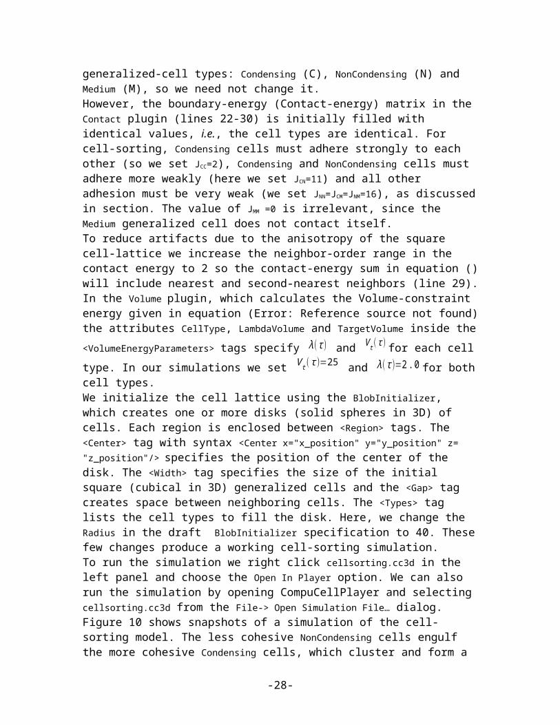
By autogenerating CC3DML code, Twedit++-CC3D releases user from remembering all the rules necessary to construct a valid CC3DML simulation script. All parameters appearing in the autogenerated CC3DML script have default values inserted by Simulation Wizard. We must edit the parameters in the draft CC3DML script to build a functional cell-sorting model (Listing 1). The CellType plugin (lines 9-13) already provides three generalized-cell types: Condensing (C), NonCondensing (N) and Medium (M), so we need not change it. However, the boundary-energy (Contact-energy) matrix in the Contact plugin (lines 22-30) is initially filled with identical values, i.e., the cell types are identical. For cell-sorting, Condensing cells must adhere strongly to each other (so we set JCC=2), Condensing and NonCondensing cells must adhere more weakly (here we set JCN=11) and all other adhesion must be very weak (we set JNN=JCM=JNM=16), as discussed in section. The value of JMM =0 is irrelevant, since the Medium generalized cell does not contact itself.
6 We highlight in yellow sections or text describing CompuCell3D behaviors which may be confusing or lead to hard-to-track errors.
-19-

t=0 MCS t=20 MCS t=880 MCS t=10000 MCS
To reduce artifacts due to the anisotropy of the square cell-lattice we increase the neighbor-order range in the contact energy to 2 so the contact-energy sum in equation () will include nearest and second-nearest neighbors (line 29). In the Volume plugin, which calculates the Volume-constraint energy given in equation (Error: Reference source not found) the attributes CellType, LambdaVolume and
TargetVolume inside the <VolumeEnergyParameters> tags specify λ (τ ) and V t (τ )for
each cell type. In our simulations we set V t (τ )=25 and λ (τ )=2. 0 for both cell types.We initialize the cell lattice using the BlobInitializer, which creates one or more disks (solid spheres in 3D) of cells. Each region is enclosed between <Region> tags. The <Center> tag with syntax <Center x="x_position" y="y_position" z= "z_position"/> specifies the position of the center of the disk. The <Width> tag specifies the size of the initial square (cubical in 3D) generalized cells and the <Gap> tag creates space between neighboring cells. The <Types> tag lists the cell types to fill the disk. Here, we change the Radius in the draft BlobInitializer specification to 40. These few changes produce a working cell-sorting simulation.To run the simulation we right click cellsorting.cc3d in the left panel and choose the Open In Player option. We can also run the simulation by opening CompuCellPlayer and selecting cellsorting.cc3d from the File-> Open Simulation File… dialog.Figure 11 shows snapshots of a simulation of the cell-sorting model. The less cohesive NonCondensing cells engulf the more cohesive Condensing cells, which cluster and form a single central domain. By changing the boundary energies we can produce other cell-sorting patterns (REF??? Glazier and Graner 1993, Graner and Glazier 1992). In particular, if we reduce the contact energy between the Condensing cell type and the Medium, we can force inverted cell sorting, where the Condensing cells surround the NonCondensing cells. If we set the heterotypic contact energy to be less than either of the homotypic contact energies, the cells of the two types will mix rather than sort. If we set the cell-medium contact energy to be very small for one cell type, the cells of that type will disperse into the medium, as in cancer invasion. With minor modifications, we can also simulate the scenarios for three or more cell types, for situations in which the cells of a given type vary in volume, motility or adhesivity, or in which the initial condition contains coherent clusters of cells rather than randomly mixed cells (engulfment).
Figure 11 Snapshots of the cell-lattice configurations for the cell-sorting simulation in Listing 1. The boundary-energy hierarchy drives NonCondensing (light grey) cells to
-20-

surround Condensing (dark grey) cells. The white background denotes surrounding Medium.
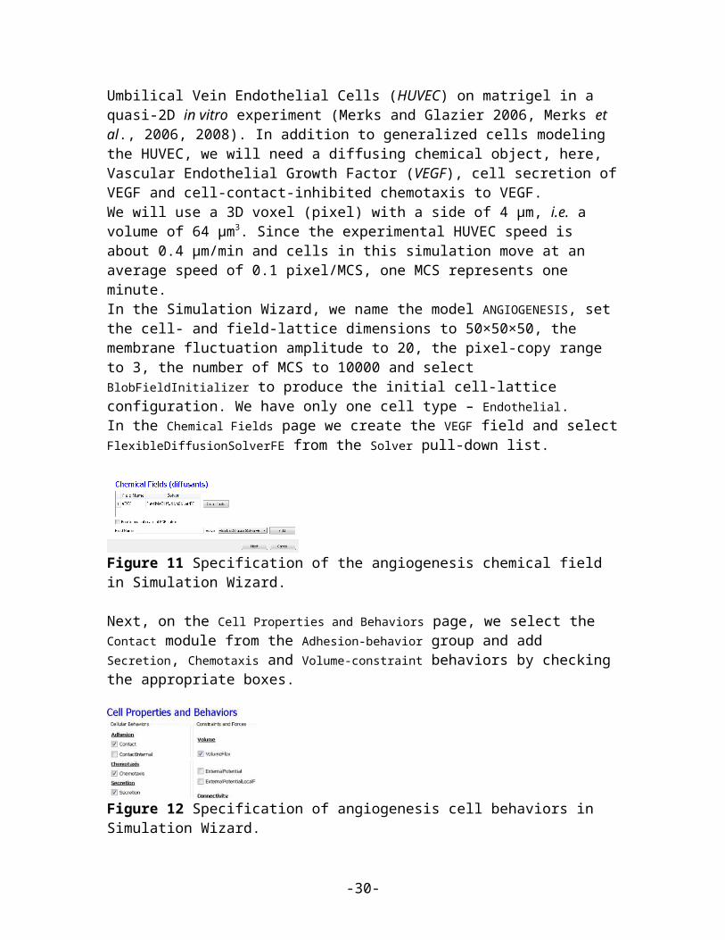
5.3 Angiogenesis ModelVascular development is central to both development and cancer progression. We present a simplified model of the earliest phases of capillary network assembly by endothelial cells based on cell adhesion and contact-inhibited chemotaxis. This model does a good job of reproducing the patterning and dynamics which occur if we culture Human Umbilical Vein Endothelial Cells (HUVEC) on matrigel in a quasi-2D in vitro experiment (Merks and Glazier 2006, Merks et al., 2006, 2008). In addition to generalized cells modeling the HUVEC, we will need a diffusing chemical object, here, Vascular Endothelial Growth Factor (VEGF), cell secretion of VEGF and cell-contact-inhibited chemotaxis to VEGF. We will use a 3D voxel (pixel) with a side of 4 µm, i.e. a volume of 64 µm3. Since the experimental HUVEC speed is about 0.4 µm/min and cells in this simulation move at an average speed of 0.1 pixel/MCS, one MCS represents one minute.In the Simulation Wizard, we name the model ANGIOGENESIS, set the cell- and field-lattice dimensions to 50×50×50, the membrane fluctuation amplitude to 20, the pixel-copy range to 3, the number of MCS to 10000 and select BlobFieldInitializer to produce the initial cell-lattice configuration. We have only one cell type – Endothelial.In the Chemical Fields page we create the VEGF field and select FlexibleDiffusionSolverFE from the Solver pull-down list.
Figure 12 Specification of the angiogenesis chemical field in Simulation Wizard.
Next, on the Cell Properties and Behaviors page, we select the Contact module from the Adhesion-behavior group and add Secretion, Chemotaxis and Volume-constraint behaviors by checking the appropriate boxes.
Figure 13 Specification of angiogenesis cell behaviors in Simulation Wizard.
Because we have invoked Secretion and Chemotaxis, the Simulation Wizard opens their configuration screens. On the Secretion page, from the pull-down list, we select the chemical to secrete by selecting VEGF in the Field pull-down menu and the cell type
-21-
secreting the chemical (Endothelial), and enter the rate of 0.013 (50 pg (cell h)-1 = 0.013 pg (voxel MCS)-1, compare to Leith and Michelson 1995). We leave the Secretion Type entry set to Uniform, so each pixel of an endothelial cell secretes the same amount of VEGF at the same rate. Uniform volumetric secretion or secretion at the cell’s center of mass may be most appropriate in 2D simulations of planar geometries (e.g. cells on a petrie dish or agar) where the biological cells are actually secreting up or down into a medium that carries the diffusant. CC3D also supplies a secrete-on-contact option to secrete outwards from the cell boundaries and allows specification of which boundaries can secrete, which is more realistic in 3D. However, users are free to employ any of these methods in either 2D or 3D depending on their interpretation of their specific biological situation. CompuCell3D does not have intrinsic units for fields, so the amount of a chemical can be interpreted in units of moles, number of molecules or grams. We click the Add Entry button to add the secretion information, then proceed to the next page to define the cells’ chemotaxis properties.
Figure 14 Specification of angiogenesis secretion parameters in Simulation Wizard.
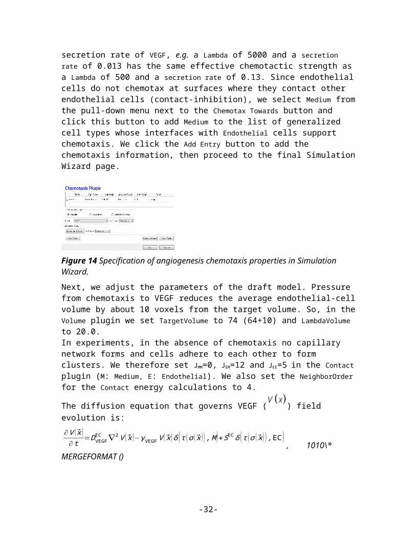
On the Chemotaxis page, we select VEGF from the Field pull-down list and Endothelial for the cell type, entering a value for Lambda of 5000. When the chemotaxis type is regular, the cell’s response to the field is linear, i.e. the effective strength of chemotaxis depends on the product of Lambda and the secretion rate of VEGF, e.g. a Lambda of 5000 and a secretion rate of 0.013 has the same effective chemotactic strength as a Lambda of 500 and a secretion rate of 0.13. Since endothelial cells do not chemotax at surfaces where they contact other endothelial cells (contact-inhibition), we select Medium from the pull-down menu next to the Chemotax Towards button and click this button to add Medium to the list of generalized cell types whose interfaces with Endothelial cells support chemotaxis. We click the Add Entry button to add the chemotaxis information, then proceed to the final Simulation Wizard page.
Figure 15 Specification of angiogenesis chemotaxis properties in Simulation Wizard.
-22-

Next, we adjust the parameters of the draft model. Pressure from chemotaxis to VEGF reduces the average endothelial-cell volume by about 10 voxels from the target volume. So, in the Volume plugin we set TargetVolume to 74 (64+10) and LambdaVolume to 20.0.In experiments, in the absence of chemotaxis no capillary network forms and cells adhere to each other to form clusters. We therefore set JMM=0, JEM=12 and JEE=5 in the Contact plugin (M: Medium, E: Endothelial). We also set the NeighborOrder for the Contact energy calculations to 4.
The diffusion equation that governs VEGF ( ) field evolution is:
∂V ( x )∂ t
=DVEGFEC ∇ 2V ( x )−γVEGF V ( x ) δ ( τ (σ ( x ) ) ,M )+SECδ ( τ (σ ( x ) ) ,EC)
, 1010\* MERGEFORMAT ()
where δ ( τ (σ ( x ) ) ,EC)=1 inside Endothelial cells and 0 elsewhere and δ ( τ (σ ( x ) ) , M )=1 inside Medium and 0 elsewhere. We set the diffusion constant =0.042 µm2/sec (0.16 voxel2/MCS, about two orders of magnitude smaller than
experimental values),7 the decay coefficient =1 h-1 [130,131] (0.016 MCS-1) for
Medium pixels and =0 inside Endothelial cells, and the secretion rate =0.013 pg (voxel MCS)-1. In the CC3DML script describing FlexibleDiffusionSolverFE (Listing 2, lines 38-47) we set the values of the <DiffusionConstant> and <DecayConstant> tags to 0.16 and 0.016 respectively. To prevent chemical decay inside Endothelial cells we add the line <DoNotDecayIn>Endothelial</DoNotDecayIn> inside the <DiffusionData> tag pair.Finally, we edit BlobInitializer (lines 49-56) to start with a solid sphere 10 pixels in radius centered at x=25, y=25, z=25 with initial cell width 4, as in Listing 2.
01 <CompuCell3D version="3.6.0">02 03 <Potts>04 <Dimensions x="50" y="50" z="50"/>05 <Steps>10000</Steps>06 <Temperature>20.0</Temperature>07 <NeighborOrder>3</NeighborOrder>08 </Potts>09 10 <Plugin Name="CellType">11 <CellType TypeId="0" TypeName="Medium"/>12 <CellType TypeId="1" TypeName="Endothelial"/>13 </Plugin>14 15 <Plugin Name="Volume">16 <VolumeEnergyParameters CellType="Endothelial" LambdaVolume="20.0" TargetVolume="74"/>17 </Plugin>18
7 FlexibleDiffusionSolverFE becomes unstable for values of >0.16 voxel2/MCS. For larger diffusion constants we must call the algorithm multiple times per MCS (See the Three-Dimensional Vascular Solid Tumor Growth section).
-23-

19 <Plugin Name="Contact">20 <Energy Type1="Medium" Type2="Medium">0</Energy>21 <Energy Type1="Medium" Type2="Endothelial">12</Energy>22 <Energy Type1="Endothelial" Type2="Endothelial">5</Energy>23 <NeighborOrder>4</NeighborOrder>24 </Plugin>25 26 <Plugin Name="Chemotaxis">27 <ChemicalField Name="VEGF" Source="FlexibleDiffusionSolverFE">28 <ChemotaxisByType ChemotactTowards="Medium" Lambda="5000.0" Type="Endothelial"/>29 </ChemicalField>30 </Plugin>31 32 <Plugin Name="Secretion">33 <Field Name="VEGF">34 <Secretion Type="Endothelial">0.013</Secretion>35 </Field>36 </Plugin>37 38 <Steppable Type="FlexibleDiffusionSolverFE">39 <DiffusionField>40 <DiffusionData>41 <FieldName>VEGF</FieldName>42 <DiffusionConstant>0.16</DiffusionConstant>43 <DecayConstant>0.016</DecayConstant>44 <DoNotDecayIn> Endothelial</DoNotDecayIn>45 </DiffusionData>46 </DiffusionField>47 </Steppable>48 49 <Steppable Type="BlobInitializer">50 <Region>51 <Center x="25" y="25" z="25"/>52 <Radius>10</Radius>53 <Width>4</Width>54 <Types>Endothelial</Types>55 </Region>56 </Steppable>57 58 </CompuCell3D>
Listing 2 CC3DML code for the angiogenesis model.
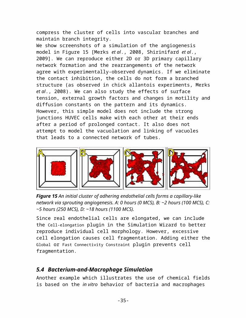
The main behavior that drives vascular patterning is contact-inhibited chemotaxis (Listing 2, lines 26-30). VEGF diffuses away from cells and decays in Medium, creating a steep concentration gradient at the interface between Endothelial cells and Medium. Because Endothelial cells chemotax up the concentration gradient only at the interface with Medium the Endothelial cells at the surface of the cluster compress the cluster of cells into vascular branches and maintain branch integrity.We show screenshots of a simulation of the angiogenesis model in Figure 16 [Merks et al., 2008, Shirinifard et al., 2009]. We can reproduce either 2D or 3D primary capillary network formation and the rearrangements of the network agree with experimentally-observed dynamics. If we eliminate the contact inhibition, the cells do not form a branched structure (as observed in chick allantois experiments, Merks et al., 2008). We can also study the effects of surface tension, external growth factors and changes in motility and diffusion constants on the pattern and its dynamics. However, this simple
-24-
model does not include the strong junctions HUVEC cells make with each other at their ends after a period of prolonged contact. It also does not attempt to model the vacuolation and linking of vacuoles that leads to a connected network of tubes.
Figure 16 An initial cluster of adhering endothelial cells forms a capillary-like network via sprouting angiogenesis. A: 0 hours (0 MCS), B: ~2 hours (100 MCS), C: ~5 hours (250 MCS), D: ~18 hours (1100 MCS).
Since real endothelial cells are elongated, we can include the Cell-elongation plugin in the Simulation Wizard to better reproduce individual cell morphology. However, excessive cell elongation causes cell fragmentation. Adding either the Global or Fast Connectivity Constraint plugin prevents cell fragmentation.
5.4 Bacterium-and-Macrophage SimulationAnother example which illustrates the use of chemical fields is based on the in vitro behavior of bacteria and macrophages in blood. In the famous experimental movie taken in the 1950s by David Rogers at Vanderbilt University, the macrophage appears to chase the bacterium, which seems to run away from the macrophage. We can model both behaviors using cell secretion of diffusible chemical signals and movement of the cells in response to the chemical (chemotaxis): the bacterium secretes a signal (a chemoattractant) that attracts the macrophage and the macrophage secretes a signal (a chemorepellant) which repels the bacterium (97). The basic procedure to construct the simulation is very similar to the one we followed in constructing angiogenesis model.
In Twedit++-CC3D we open new project and name it bacterium_macrophage. We declare 3 cell types – Bacterium, Macrophage and Red (red blood cells). We assume that diffusing chemoattractant is secreted by bacteria, therefore on the Chemical Field page of the Simulation Wizard we declare ATTR chemical field which we will solve using DiffusionSolverFE. On the Cell Behaviors and Properties page we select Contact, Chemotaxis, VolumeFlex and Surface Flex. Clicking ‘Next’ button brings us to chemotaxis page where we set chemotaxis parameters as shown on Figure 17:
-25-
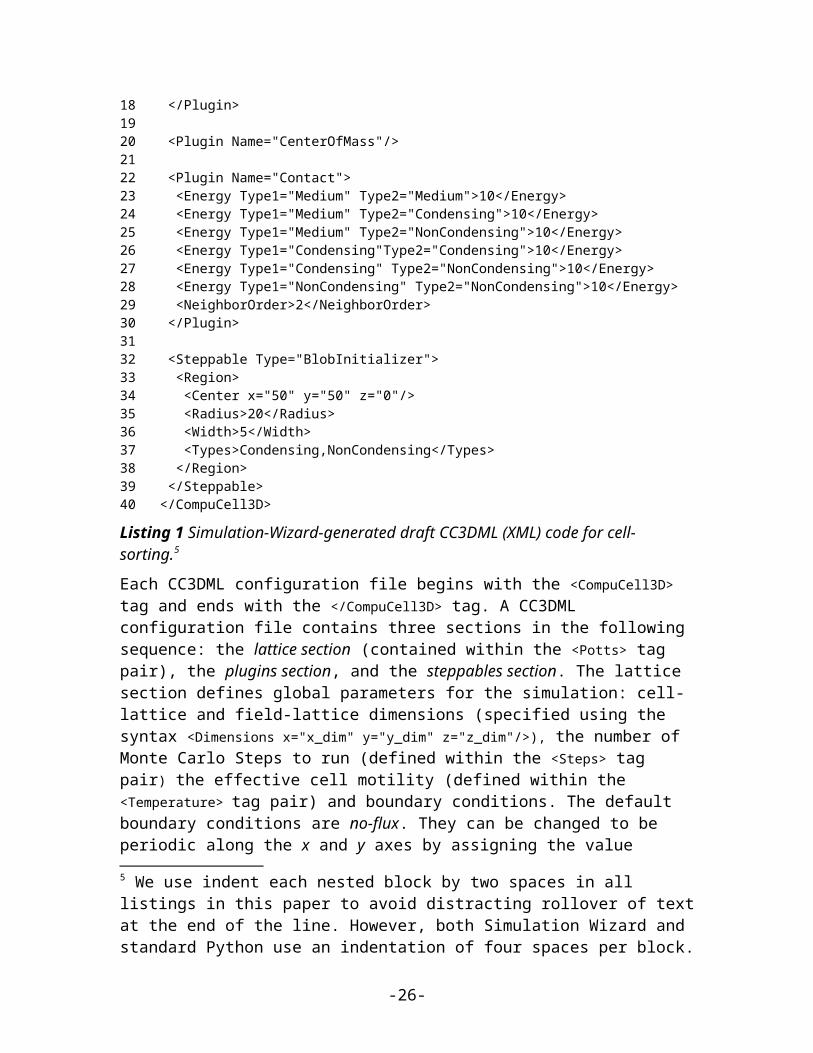
Figure 17 Setting up chemotaxis properties forMacrophages
After code-autogenerating is done we have to do several adjustments to the CC3DML script.
01 <CompuCell3D version="3.6.2">02 03 <Potts> 04 <Dimensions x="100" y="100" z="1"/>05 <Steps>10000</Steps>06 <Temperature>40.0</Temperature>07 <NeighborOrder>2</NeighborOrder>08 <Boundary_x>Periodic</Boundary_x>09 <Boundary_y>Periodic</Boundary_y>10 </Potts>11 12 <Plugin Name="CellType"> 13 <CellType TypeId="0" TypeName="Medium"/>14 <CellType TypeId="1" TypeName="Bacterium"/>15 <CellType TypeId="2" TypeName="Macrophage"/>16 <CellType TypeId="3" TypeName="Red"/>17 </Plugin>18 19 <Plugin Name="Volume">20 <VolumeEnergyParameters CellType="Bacterium" LambdaVolume="60.0" TargetVolume="10"/>21 <VolumeEnergyParameters CellType="Macrophage" LambdaVolume="15.0" TargetVolume="150"/>22 <VolumeEnergyParameters CellType="Red" LambdaVolume="30.0" TargetVolume="100"/>23 </Plugin>24 25 <Plugin Name="Surface">26 <SurfaceEnergyParameters CellType="Bacterium" LambdaSurface="4.0" TargetSurface="10"/>27 <SurfaceEnergyParameters CellType="Macrophage" LambdaSurface="20.0" TargetSurface="50"/>28 <SurfaceEnergyParameters CellType="Red" LambdaSurface="0.0" TargetSurface="40"/>29 </Plugin>30 31 <Plugin Name="Contact"> 32 <Energy Type1="Medium" Type2="Medium">10.0</Energy>33 <Energy Type1="Medium" Type2="Bacterium">8.0</Energy>34 <Energy Type1="Medium" Type2="Macrophage">8.0</Energy>35 <Energy Type1="Medium" Type2="Red">30.0</Energy>36 <Energy Type1="Bacterium" Type2="Bacterium">150.0</Energy>37 <Energy Type1="Bacterium" Type2="Macrophage">15.0</Energy>38 <Energy Type1="Bacterium" Type2="Red">150.0</Energy>39 <Energy Type1="Macrophage" Type2="Macrophage">150.0</Energy>40 <Energy Type1="Macrophage" Type2="Red">150.0</Energy>41 <Energy Type1="Red" Type2="Red">150.0</Energy>42 <NeighborOrder>2</NeighborOrder>43 </Plugin>44 45 <Plugin Name="Chemotaxis">46 <ChemicalField Name="ATTR" Source="DiffusionSolverFE">47 <ChemotaxisByType Lambda="1.0" Type="Macrophage"/>48 </ChemicalField>
-26-

49 </Plugin>50 51 <Steppable Type="DiffusionSolverFE">52 <DiffusionField>53 <DiffusionData>54 <FieldName>ATTR</FieldName>55 <GlobalDiffusionConstant>0.1</GlobalDiffusionConstant>56 <GlobalDecayConstant>5e-05</GlobalDecayConstant>57 <DiffusionCoefficient CellType="Red">0.0</DiffusionCoefficient>58 </DiffusionData>59 <SecretionData>60 <Secretion Type="Bacterium">100</Secretion>61 </SecretionData>62 <BoundaryConditions>63 <Plane Axis="X">64 <Periodic/>65 </Plane>66 <Plane Axis="Y">67 <Periodic/>68 </Plane>69 </BoundaryConditions>70 </DiffusionField>71 </Steppable>72 73 <Steppable Type="PIFInitializer">74 <PIFName>Simulation/bacterium_macrophage.piff</PIFName>75 </Steppable>76 77 </CompuCell3D>78
Listing 3. CC3DML code for Bacterium Macrophage simulation. Note that the code has been modified from its autogenetrated version
We implement the actual bacterium-macrophage “chasing” mechanism using the Chemotaxis plugin, which specifies how a generalized cell of a given type responds to a field. The Chemotaxis plugin biases a cell’s motion up or down a field gradient by changing the calculated effective-energy change used in the acceptance function,
equation 8. For a field :
1111\*MERGEFORMAT ()
where is the chemical field at the index-copy target pixel, the field at the
index-copy source pixel, and the strength and direction of chemotaxis. If
and , then is negative, increasing the probability of accepting the index copy in equation 8. The net effect is that the cell moves up the field gradient with a
velocity . If λ<0 is negative, the opposite occurs, and the cell will move down
the field gradient. Plugins with more sophisticated calculations (e.g., including
-27-
che
chem c m
m
he
0
H c i c i
c i
x
response saturation) are available within CompuCell3D (see the description of the chemotaxis plugin in the second part of this manual).
Figure 18. Connecting a field to GGH dynamics using a chemotaxis-energy term. The difference in the value of the field at the source, , and target, , pixels changes the
of the index-copy attempt. Here and , so , increasing the probability of accepting the index-copy attempt in equation 8.
In the Chemotaxis plugin we must identify the names of the fields, where the field information is stored, the list of the generalized-cell types that will respond to the fields,
and the strength and direction of the response (Lambda = ). The information for each field is specified using the syntax:<ChemicalField Source="where field is stored" Name="field name"> <ChemotaxisByType Type="cell_type1" Lambda="lambda1"/> <ChemotaxisByType Type="cell_type2" Lambda="lambda1"/> </ChemicalField>
In our current example, the first field, named ATTR, is stored in
DiffusionSolverFE. Macrophage cells are attracted to ATTR with . None of the other cell types responds to ATTR. Similarly, Bacterium cells are repelled
by REP with .
Keep in mind that fields are not created within the Chemotaxis plugin, which only specifies how different cell types respond to the fields. We define and store the fields elsewhere. Here, we use the DiffusionSolverFE steppable as the source of our fields. The DiffusionSolverFE steppable is the main CompuCell3D tool for defining diffusing fields, which evolve according to the diffusion equation:
, 1212\*MERGEFORMAT ()
-28-

where is the field concentration and , and denote the diffusion constant (in m2/s), decay constant (in s-1) and secretion rates (in concentration/s) of the
field, respectively. , , and s( i ) may vary with position and cell-lattice configuration.
As in the Chemotaxis plugin, we may define the behaviors of multiple fields, enclosing each one within <DiffusionField> tag pairs. For each field defined within a <DiffusionData> tag pair, users provide values for the name of the field (using the <FieldName> tag pair), the global diffusion constant (using the <GlobalDiffusionConstant> tag pair) , and the global decay constant (using the <GlobalDiffusionConstant> tag pair). We can also specify diffusion constant for particular cell types using the following syntax:<DiffusionCoefficient CellType="cell_type_1">coefficient</DiffusionCoefficient><DecayCoefficient CellType="cell_type_1">coefficient</DecayCoefficient>
Forward-Euler methods are numerically unstable for large diffusion constants, limiting the maximum nominal diffusion constant allowed in CompuCell3D simulations. However, by increasing the PDE-solver calling frequency, which reduces the effective time step, CompuCell3D can simulate arbitrarily large diffusion constants and using the DiffusionSolverFE to solve diffusion equation releases users from specifying how many extra times the solver needs to be called.
The optional <SecretionData> tag pair defines a subsection which identifies cells types that secrete or absorb the field and the rates of secretion:<SecretionData> <Secretion Type="cell_type1">real_rate1</Secretion> <Secretion Type="cell_type2">real_rate2</Secretion><SecretionData>
A negative rate simulates absorption. In the bacterium and macrophage simulation, Bacterium cells secrete ATTR.
To complete specification of the PDE diffusion equation we also set boundary conditions (by default they are set to no flux). Here however we set them to Periodic along x and y directions using the following syntax:<BoundaryConditions> <Plane Axis="X"> <Periodic/> </Plane> <Plane Axis="Y"> <Periodic/> </Plane></BoundaryConditions>
We load the initial configuration for the bacterium-and-macrophage simulation using the PIFInitializer steppable. Many simulations require initial generalized-cell configurations that we cannot easily construct from primitive regions filled with cells using BlobInitializer and UniformInitializer. To allow maximum flexibility, CompuCell3D can read the initial cell-lattice configuration from Pixel Initialization Files (PIFFs). A PIFF is a text file that allows users to assign multiple rectangular (parallelepiped in 3D) pixel regions or single pixels to particular cells.
-29-
Each line in a PIF has the syntax:Cell_id Cell_type x_low x_high y_low y_high z_low z_highwhere Cell_id is a unique cell index. A PIF may have multiple, possibly non-adjacent, lines starting with the same Cell_id; all lines with the same Cell_id define pixels of the same generalized cell. The values x_low, x_high, y_low, y_high, z_low and z_high define rectangles (parallelepipeds in 3D) of pixels belonging to the cell. In the case of overlapping pixels, a later line overwrites pixels defined by earlier lines. The following line describes a 6 x 6-pixel square cell with cell index 0 and type Amoeba:0 Amoeba 10 15 10 15 0 0
If we save this line to the file 'amoebae.piff', we can load it into a simulation using the following syntax:<Steppable Type="PIFInitializer"> <PIFName>amoebae.piff</PIFName> </Steppable>
Listing 4 illustrates how to construct arbitrary shapes using a PIF. Here we define two cells with indices 0 and 1, and cell types Amoeba and Bacterium, respectively. The main body of each cell is a 6 x 6 square to which we attach additional pixels.
0 Amoeba 10 15 10 15 0 01 Bacterium 25 30 25 30 0 00 Amoeba 16 16 15 15 0 01 Bacterium 25 27 31 35 0 0
Listing 4. Simple PIF initializing two cells, one each of type Bacterium and Amoeba.
All lines with the same cell index (first column) define a single cell. Figure 19 shows the initial cell-lattice configuration specified in Listing 4:
Figure 19. Initial configuration of the cell lattice based on the PIF in Listing 4.
In practice, because constructing complex PIFs by hand is cumbersome, we generally use custom-written scripts to generate the file directly, or convert images stored in graphical formats (e.g., gif, jpeg, png) from experiments or other programs.
Listing 5 shows the example PIF for the bacterium-and-macrophage simulation.
-30-

0 Red 10 20 10 20 0 01 Red 10 20 40 50 0 02 Red 10 20 70 80 0 03 Red 40 50 0 10 0 04 Red 40 50 30 40 0 05 Red 40 50 60 70 0 06 Red 40 50 90 95 0 07 Red 70 80 10 20 0 08 Red 70 80 40 50 0 09 Red 70 80 70 80 0 011 Bacterium 5 5 5 5 0 012 Macrophage 35 35 35 35 0 0 13 Bacterium 65 65 65 65 0 014 Bacterium 65 65 5 5 0 015 Bacterium 5 5 65 65 0 016 Macrophage 75 75 95 95 0 0 17 Red 24 28 10 20 0 018 Red 24 28 40 50 0 019 Red 24 28 70 80 0 020 Red 40 50 14 20 0 021 Red 40 50 44 50 0 022 Red 40 50 74 80 0 023 Red 54 59 90 95 0 024 Red 70 80 24 28 0 025 Red 70 80 54 59 0 026 Red 70 80 84 90 0 027 Macrophage 10 10 95 95 0 0
Listing 5. PIF defining the initial cell-lattice configuration for the bacterium-and-macrophage simulation. The file is stored as 'bacterium_macrophage_2D_wall_v3.pif'.
In Error: Reference source not found we read the cell lattice configuration from the file 'bacterium_macrophage_2D_wall_v3.pif' using the lines:<Steppable Type="PIFInitializer"> <PIFName>Simulation/bacterium_macrophage.piff</PIFName> </Steppable>
Figure 20 shows snapshots of the bacterium-and-macrophage simulation. By adjusting the properties and number of bacteria, macrophages and red blood cells and the diffusion properties of the chemical fields, we can build a surprisingly good reproduction of the experiment.
-31-
t=200 MCS t=500 MCS t=800 MCS t=900 MCS t=1100 MCS
Figure 20. Snapshots of the bacterium-and-macrophage simulation from Error: Reference source not found and the PIF in Listing 5 saved in the file 'bacterium_macrophage_2D_wall_v3.pif'. The upper row shows the cell-lattice configuration with the Macrophages in grey, Bacteria in white, red blood cells in dark grey and Medium in blue. Second row shows the concentration of the chemoattractant ATTR secreted by the Bacteria. The bars at the bottom of the field images show the concentration scales (blue, low concentration, red, high concentration).
6 Python ScriptingCC3DML is convenient for building simple simulations such as those we presented above. To describe more complex simulations, CompuCell3D allows users to write specialized, shareable modules in C/C++ (through the CompuCell3D Application Programming Interface, or CC3D API) or Python (through a Python-scripting interface). C and C++ modules have the advantage that they run at native speed. However, developing them requires knowledge of both C/C++ and the CC3D API, and their integration with CompuCell3D requires recompilation of the source code. Python module development is less complicated, since Python has simpler syntax than C/C++ and users can modify and extend a library of Python-module templates included with CompuCell3D. Moreover, Python modules do not require recompilation.
Tasks performed by CompuCell3D modules either relate to index-copy attempts (plugins) or run either once, at the beginning or end of a simulation, or once every several MCS (steppables). Tasks run every index-copy attempt, like effective-energy-term calculations, are the most frequently-called tasks in a GGH simulation and writing them in Python may slow simulations. However, steppables and lattice monitors are good candidates for Python implementation and cause negligible performance degradation. Python implementations are suitable for most cell-parameter adjustments that depend on the state of the simulation, e.g., simulating cell growth in response to a chemical, cell-type differentiation and changes in cell-cell adhesion.
-32-

In the models we presented above, all cells had parameter values fixed in time. To allow cell behaviors to change, we need to be able to adjust cell properties during a simulation. CompuCell3D can execute Python scripts (CC3D supports Python versions 2.x) to modify the properties of cells in response to events occurring during a simulation, such as the concentration of a nutrient dropping below a threshold level, a cell reaching a doubling volume or a cell changing its neighbors. Most such Python scripts have a simple structure based on print statements, if-elif-else statements, for loops, lists and simple classes and do not require in-depth knowledge of Python to create.
6.1 A Short Introduction to Python
This section briefly introduces the main features of Python in the CompuCell3D context. For a more formal introduction to Python see Lutz 2011 and http://python.org.Python defines blocks of code, such as those appearing inside if statements or for loops (in general after “:”), by an increased level of indentation. This chapter uses 2 spaces per indentation level. For example, in Listing 3, we indent the body of the if statement by 2 spaces and the body of the inner for loop by an additional 2 spaces. The for loop is executed inside the if statement, which checks if we are in the second MCS of the simulation. The command pixelOffset=10 assigns to the variable pixelOffset a value of 10. The for loop assigns to the variable x values ranging from 0 through self.dim.x-1, where self.dim.x is a CC3D internal variable containing the size of the cell-lattice in the x-direction. When executed, Listing 3 prints consecutive integers from 10 to 10+self.dim.x-1.
01 if (mcs==2):02 pixelOffset = 1003 for x in range(self.dim.x):04 pixel = pixelOffset + x 05 print pixel
Listing 6 Simple Python loop.
The great advantage of Python compared to older languages like Fortran is that it can also iterate over members of a Python list, a container for grouping objects. Listing 4 executes a for loop over a list containing all cells in the simulation and prints the type of each cell.
01 for cell in self.cellList:02 print ”cell type=”, cell.type
Listing 7 Iterating over the inventory of CC3D cells in Python.
Lists can combine objects of any type, including integers, strings, complex numbers, lists, and, in this case, CC3D cells. CompuCell3D uses lists extensively to keep track of cells, cell neighbors, cell pixels, etc.…. CompuCell3D allows users to construct custom Python code as independent modules called steppables, which are represented as classes. Listing 5 shows a typical CC3D Python steppable class. The first line declares the class name together with an argument (SteppableBasePy) inside the parenthesis which makes the main CC3D objects, including cells, lattice properties, etc.…, available inside the class. The def __init__( self,_simulator,_frequency=1): declares the initializing function __init__ which is
-33-

called automatically during class object instantiation. After initializing the class and inheriting CC3D objects, we declare 3 main functions called at different times during the simulation: start is called before the simulation starts; step is called at specified intervals in MCS throughout the simulation; and finish is called at the end of the simulation. The start function iterates over all cells, setting their target volume and inverse compressibility to 25 and 5, respectively. Generically, we use the start function to define model initial conditions. The step function increases the target volumes of all cells by 0.001 after the tenth MCS, a typical way to implement cell growth in CC3D. The finish function prints the cell volumes at the end of the simulation.
01 class Example(SteppableBasePy):02 def __init__(self,_simulator,_frequency=1):03 SteppableBasePy.__init__(self,_simulator,_frequency)04 05 def start(self):06 print “Called at the beginning of the simulation” 07 for cell in self.cellList:08 cell.targetVolume=2509 cell.lambdaVolume=510 11 def step(self,mcs):12 print “Called every MCS”13 if (mcs>10):14 for cell in self.cellList:15 cell.targetVolume+=0.00116 17 def finish(self):18 print “Called at the end of the simulation”19 for cell in self.cellList:20 print “cell volume = ”, cell.volume
Listing 8 Sample CC3D steppable class.
start, step and finish functions have default implementations in the base class SteppableBasePy. Therefore we only need to provide definition of those functions which we want to override. In addition, we can add our own functions to the class. The next section uses Python scripting to build a complex CompuCell3D model.
6.2 General structure of CC3D Python scriptsPython scripting allows users to augment their CC3DML configuration files with Python scripts or to code their entire simulations in Python (in which case the Python script looks very similar to the CC3DML script it replaces). Error: Reference source not found shows the standard block of template code for running a Python script in conjunction with a CC3DML configuration file.import sysfrom os import environfrom os import getcwdimport stringsys.path.append(environ["PYTHON_MODULE_PATH"])import CompuCellSetup
sim,simthread = CompuCellSetup.getCoreSimulationObjects()
#Create extra player fields here or add attributes
-34-
CompuCellSetup.initializeSimulationObjects(sim,simthread)
#Add Python steppables heresteppableRegistry=CompuCellSetup.getSteppableRegistry()
#Steppable registrationfrom CustomSteppables import CustomSteppablecustomSteppableInstance= CustomSteppable (sim,_frequency=100)steppableRegistry.registerSteppable(customSteppableInstance)
CompuCellSetup.mainLoop(sim,simthread,steppableRegistry)
Listing 9. Basic Python template to run a CompuCell3D simulation through a Python interpreter. Later examples will be based on this script.
The import sys line provides access to standard functions and variables needed to manipulate the Python runtime environment. The next two lines, from os import environfrom os import getcwd
import environ and getcwd housekeeping functions into the current namespace (i.e., current script) and are included in all our Python programs. In the next three lines, import stringsys.path.append(environ["PYTHON_MODULE_PATH"])import CompuCellSetup
we import the string module, which contains convenience functions for performing operations on strings of characters, set the search path for Python modules and import the CompuCellSetup module, which provides a set of convenience functions that simplify initialization of CompuCell3D simulations.
Next, we create and initialize the core CompuCell3D modules:sim,simthread = CompuCellSetup.getCoreSimulationObjects()CompuCellSetup.initializeSimulationObjects(sim,simthread)
We then create a steppable registry (a Python container that stores steppables, i.e., a list of all steppables that the Python code can access) and pass it to the function that runs the simulation:steppableRegistry=CompuCellSetup.getSteppableRegistry()
#Steppable registrationfrom CustomSteppables import CustomSteppablecustomSteppableInstance= CustomSteppable (sim,_frequency=100)steppableRegistry.registerSteppable(customSteppableInstance)
CompuCellSetup.mainLoop(sim,simthread,steppableRegistry)
Here we show example of how to instantiate and register a steppable (CustomSteppable). CustomSteppable is stored in file CustomSteppables.py and we import its content by typing:from CustomSteppables import CustomSteppable
When Twedit++ generates simulation scripts the above script is generated automatically and it rarely needs any modifications.
In the next section, we will explain how to modify autogenerated steppable to implement dynamically changing cell properties.
-35-

6.3 Cell-Type-Oscillator SimulationSuppose that we would like to add a caricature of oscillatory gene expression to our cell-sorting simulation so that cells exchange types every 100 MCS. All we have to do in is to then is to generate in Twedit++ cellsorting simulation but making sure that on the first page of the wizard screen we choose Python+XML option. As a result we will get simulation scripts (CC3DML and Python) which we will modify to create this simple new simulation. We will implement the changes of cell types using a Python steppable, since it occurs at intervals of 100 MCS. The skeleton of the steppable is autogenerated by Twedit++ and Listing 10 shows the modification which are needed to turn boiler-plate code into functional simulation:from PySteppables import *import CompuCellimport sysclass CellTypeOscillatorSteppable(SteppableBasePy):
def __init__(self,_simulator,_frequency=10): SteppableBasePy.__init__(self,_simulator,_frequency) def step(self): print ”START FUNCTION” def step(self,mcs): for cell in self.cellList: if cell.type==self.CONDENSING: cell.type=self.NONCONDENSING elif cell.type==self.NONCONDENSING: cell.type=self.CONDENSING def finish(self): print ”FINISH FUNCTION”
Listing 10. Autogenerated Python steppable with modification necessary to implement oscillatory cell type switching. The changes to to script are indicated in bold font.
A CompuCell3D steppable is a class (a type of object) that holds the parameters and functions necessary for carrying out a task. Every steppable defines at least 4 functions: __init__(self, _simulator, _frequency), start(self), step(self, mcs) and finish(self).
CompuCell3D calls the start(self) function once at the beginning of the simulation before any index-copy attempts. It calls the step(self, mcs) function periodically after every _frequency MCS. It calls the finish(self) function once at the end of the simulation. Error: Reference source not found does not have explicit start(self) or finish(self) functions. Instead, the class definition :class CellTypeOscillatorSteppable (SteppableBasePy):
causes the TypeSwitcherSteppable to inherit components of the SteppableBasePy class. SteppableBasePy contains default definitions of the start(self), step(self,mcs) and finish(self) functions as well as many othr convenience objects such as e.g. cellList. Inheritance reduces the length of the user-written Python code
-36-

and ensures that the CellTypeOscillatorSteppable object has all needed components. The line:from PySteppables import *
makes the content of 'PySteppables.py' file (or module) available in the current namespace. The PySteppables module includes the SteppableBasePy base class.
The __init__ function is a constructor that accepts user-defined parameters and initializes a steppable object. Consider the __init__ function of the TypeSwitcherSteppable:def __init__(self,_simulator,_frequency=100): SteppablePy.__init__(self,_frequency)
Here we call the constructor for the inheritance class, SteppableBasePy, as required by Python. This instantiates many convenience objects which are available from within our CellTypeOscillatorSteppable class. For example we can write self.simulator to reference to simulator object, passed from the main script or by typing self.cellList we access a reference to cell inventory managed by CC3D kernel. We can think about Python reference as a pointer variable that stores the address of the object but not a copy of the object itself. Cell inventory allows us to visit all the cells with a simple for loop to perform various tasks. The cell inventory is a dynamic structure, i.e., it updates automatically when cells are created or destroyed during a simulation.
The section of the CellTypeOscillatorSteppable steppable which implements the cell-type switching is found in the step(self, mcs) function: def step(self,mcs): for cell in self.cellList: if cell.type==self.CONDENSING: cell.type=self.NONCONDENSING elif cell.type==self.NONCONDENSING: cell.type=self.CONDENSING
Here we use the cell inventory to iterate over all cells in the simulation and reassign their cell types between self.CONDENSING and self.NONCONDENSING. are constants which are equal to id’s of cell types in our simulation (recall that cellsording had two cell types Condensing and NonCondensing). The names of the constants can be easily created from type name by capitalizing all the letters and prepending them with self. – for exampleNonCondensing self.NONCONDENSING
Once we have created a steppable (i.e., created an object of class CellTypeOscillatorSteppable) we must register it using registerSteppable function from steppableRegistry object:from CellTypeOscillatorSteppables import CellTypeOscillatorSteppablesteppableInstance=CellTypeOscillatorSteppable(sim,_frequency=100)steppableRegistry.registerSteppable(steppableInstance)
CompuCell3D will not run unregistered steppables.
Figure 21 shows snapshots of the cell-type-oscillator simulation.
-37-
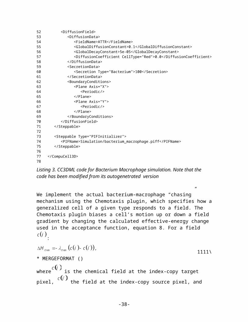
t=90 MCS t=110 MCS t=1490 MCS t=1510 MCS
Figure 21. Results of the Python cell-type-oscillator simulation using the TypeSwitcherSteppable steppable implemented in Error: Reference source not found in conjunction with the CC3DML cell-sorting simulation. Cells exchange types and corresponding adhesivities and colors every 100 MCS; i.e., between t=90 MCS and t=110 MCS and between t=1490 MCS and t=1510 MCS.
We mentioned earlier that users can run simulations without a CC3DML configuration file. The easiest and fastes way to convert CC3DML to equivalent Python syntax is to use Twedit++. By right-clicking on a CC3MDL file tag in the CC3D Project panel we get access to context menu “Convert XML to Python”. By choosing it , with one click we convert entire CC3DML to Python syntax as shown
Figure 22 Converting CC3DML to Python syntax.
Listing 11 shows the cell-type-oscillator simulation written entirely in Python, with changes to Error: Reference source not found shown in bold.
def configureSimulation(sim): import CompuCellSetup from XMLUtils import ElementCC3D CompuCell3DElmnt=ElementCC3D("CompuCell3D",{"version":"3.6.2"}) PottsElmnt=CompuCell3DElmnt.ElementCC3D("Potts") # Basic properties of CPM (GGH) algorithm PottsElmnt.ElementCC3D("Dimensions",{"x":"100","y":"100","z":"1"}) PottsElmnt.ElementCC3D("Steps",{},"10000")
-38-

PottsElmnt.ElementCC3D("Temperature",{},"10.0") PottsElmnt.ElementCC3D("NeighborOrder",{},"2") PluginElmnt=CompuCell3DElmnt.ElementCC3D("Plugin",{"Name":"CellType"}) # Listing all cell types in the simulation PluginElmnt.ElementCC3D("CellType",{"TypeId":"0","TypeName":"Medium"}) PluginElmnt.ElementCC3D("CellType",{"TypeId":"1","TypeName":"Condensing"}) PluginElmnt.ElementCC3D("CellType",{"TypeId":"2","TypeName":"NonCondensing"}) PluginElmnt_1=CompuCell3DElmnt.ElementCC3D("Plugin",{"Name":"Volume"}) PluginElmnt_1.ElementCC3D("VolumeEnergyParameters",\ {"CellType":"Condensing","LambdaVolume":"2.0","TargetVolume":"25"}) PluginElmnt_1.ElementCC3D("VolumeEnergyParameters",\ {"CellType":"NonCondensing","LambdaVolume":"2.0","TargetVolume":"25"}) PluginElmnt_2=CompuCell3DElmnt.ElementCC3D("Plugin",{"Name":"NeighborTracker"}) # Module tracking center of mass of each cell PluginElmnt_3=CompuCell3DElmnt.ElementCC3D("Plugin",{"Name":"Contact"}) # Specification of adhesion energies PluginElmnt_3.ElementCC3D("Energy",{"Type1":"Medium","Type2":"Medium"},"10.0") PluginElmnt_3.ElementCC3D("Energy",{"Type1":"Medium","Type2":"Condensing"},"16.0") PluginElmnt_3.ElementCC3D("Energy",{"Type1":"Medium","Type2":"NonCondensing"},"16.0") PluginElmnt_3.ElementCC3D("Energy",{"Type1":"Condensing","Type2":"Condensing"},"2.0") PluginElmnt_3.ElementCC3D("Energy",\ {"Type1":"Condensing","Type2":"NonCondensing"},"11.0") PluginElmnt_3.ElementCC3D("Energy",\ {"Type1":"NonCondensing","Type2":"NonCondensing"},"15.0") PluginElmnt_3.ElementCC3D("NeighborOrder",{},"2") SteppableElmnt=CompuCell3DElmnt.ElementCC3D("Steppable",{"Type":"BlobInitializer"}) # Initial layout of cells in the form of spherical (circular in 2D) blob RegionElmnt=SteppableElmnt.ElementCC3D("Region") RegionElmnt.ElementCC3D("Center",{"x":"50","y":"50","z":"0"}) RegionElmnt.ElementCC3D("Radius",{},"40") RegionElmnt.ElementCC3D("Gap",{},"0") RegionElmnt.ElementCC3D("Width",{},"5") RegionElmnt.ElementCC3D("Types",{},"Condensing,NonCondensing")
-39-
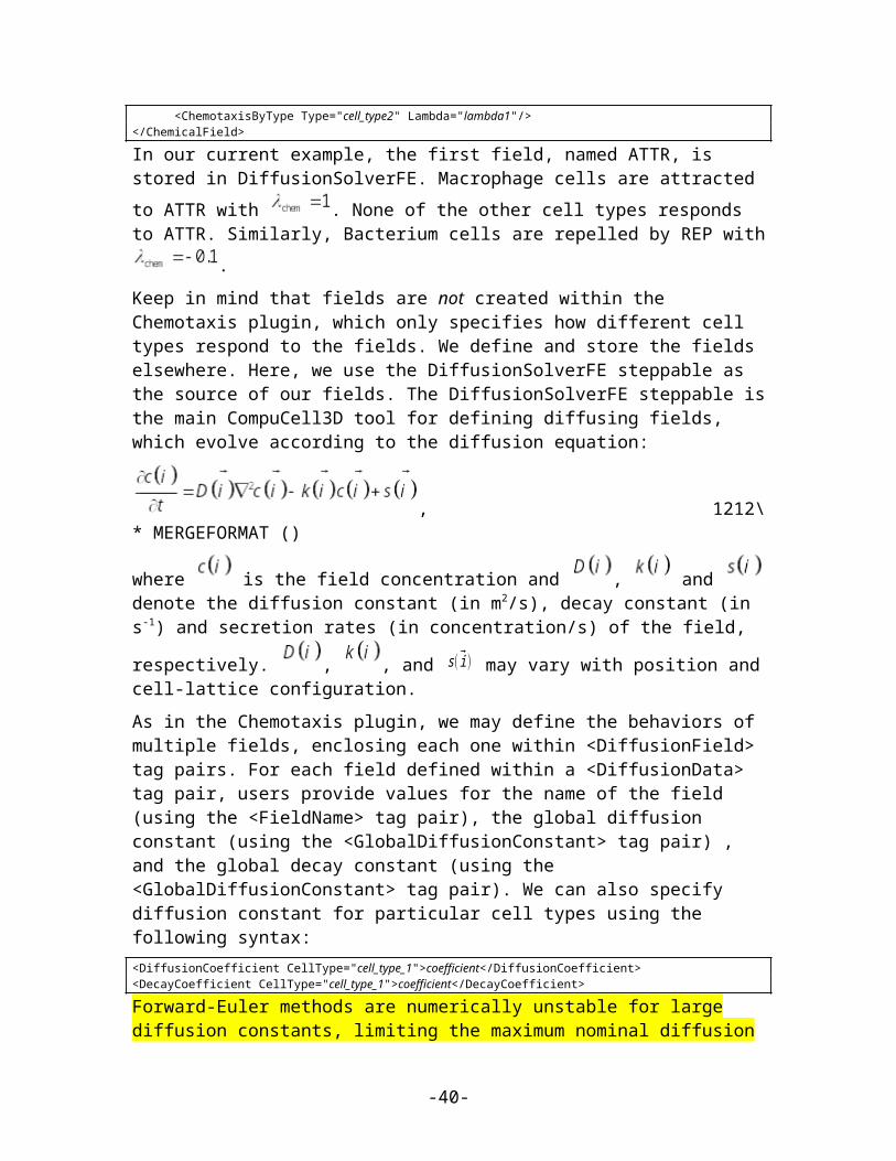
CompuCellSetup.setSimulationXMLDescription(CompuCell3DElmnt) import sysfrom os import environfrom os import getcwdimport string
sys.path.append(environ["PYTHON_MODULE_PATH"])
import CompuCellSetup
sim,simthread = CompuCellSetup.getCoreSimulationObjects() configureSimulation(sim) # add extra attributes here CompuCellSetup.initializeSimulationObjects(sim,simthread)# Definitions of additional Python-managed fields go here #Add Python steppables heresteppableRegistry=CompuCellSetup.getSteppableRegistry() from CellTypeOscillatorSteppables import CellTypeOscillatorSteppablesteppableInstance=CellTypeOscillatorSteppable(sim,_frequency=100)steppableRegistry.registerSteppable(steppableInstance) CompuCellSetup.mainLoop(sim,simthread,steppableRegistry)Listing 11. Stand-alone Python cell-type-oscillator script containing an initial section that replaces the CC3DML from Listing 1.
The configureSimulation function replaces the CC3DML file from Listing 1. After importing CompuCell and CompuCellSetup, we have access to functions and modules that provide all the functionality necessary to code a simulation in Python. The conversion from XML to Python follows simple algorithm for nested data structures and is explained in detail in Python Scripting Manual. In essentially all cases users never need to bother with the details of this algorithm as Twedit++ does all the work behind the scenes. Great advantage of using Python-only simulations is that parameters appearing in the configureSim function (this function replaces the CC3DML script) can be Python variables or Python expressions and this may help users in building simulation codes which are easit to maintain.
6.4 Diffusing-Field-Based Cell-Growth SimulationOne of the most frequent uses of Python scripting in CompuCell3D simulations is to modify cell behavior based on local field concentrations. To demonstrate this use, we incorporate stem-cell-like behavior into the cell-sorting simulation from Listing 1. This extension requires including relatively sophisticated interactions between cells and diffusing chemical, FGF (100). However the implmenetation of those behavior in CC3D is relatively straightforward as we will show.
-40-

We simulate a situation where NonCondensing cells secrete FGF, which diffuses freely through the cell lattice and obeys:
, 1313\* MERGEFORMAT ()
where denotes the FGF concentration and Condensing cells respond to the field by growing at a constant rate proportional to the FGF concentration at their centroids:dV t (s )
dt=0 . 01[ FGF ]( xs )
. 1414\* MERGEFORMAT ()
When they reach a threshold volume, the Condensing cells undergo mitosis. One of the resulting daughter cells remains a Condensing cell, while the other daughter cell has an equal probability of becoming either another Condensing cell or a DifferentiatedCondensing cell. DifferentiatedCondensing cells do not divide.
Each generalized cell in CompuCell3D has a default list of attributes, e.g. type, volume, surface (area), target volume, etc.. However, CompuCell3D allows users to add cell attributes during execution of simulations. E.g., in the current simulation, we will record data on each cell division in a list attached to each cell. Generalized cell attributes can be added using either C++ or Python. However, attributes added using Python are not accessible from C++ modules.
We start constructing our simulation by invoking CC3D Simulation Wizard from Twedit++ and naming simulation cellsort_2D_field. We set lattice dimension to 200x200x1, number of steps to 300 and NeighborOrder to 3. We then declare 3 cell types Condensing, NonCondensing and DifferentiatedCondensing. On the Chemical Fields page we declare one diffusant - FGF and choose DiffusionSolverFE to evolve the field. On the Cell Properties and Behaviors page we check Contact, VolumeLocalFlex and Mitosis and complete wizard workflow by clicking next until we get to final page which generates simulation template.
First thing we do with autogenerated code we edit CC3DML file as follows (changes are shown in bold):
<CompuCell3D version="3.6.2"> <Potts> <Dimensions x="200" y="200" z="1"/> <Steps>3000</Steps> <Temperature>10.0</Temperature> <NeighborOrder>2</NeighborOrder> </Potts> <Plugin Name="CellType"> <CellType TypeId="0" TypeName="Medium"/> <CellType TypeId="1" TypeName="Condensing"/> <CellType TypeId="2" TypeName="NonCondensing"/> <CellType TypeId="3" TypeName="DifferentiatedCondensing"/>
-41-
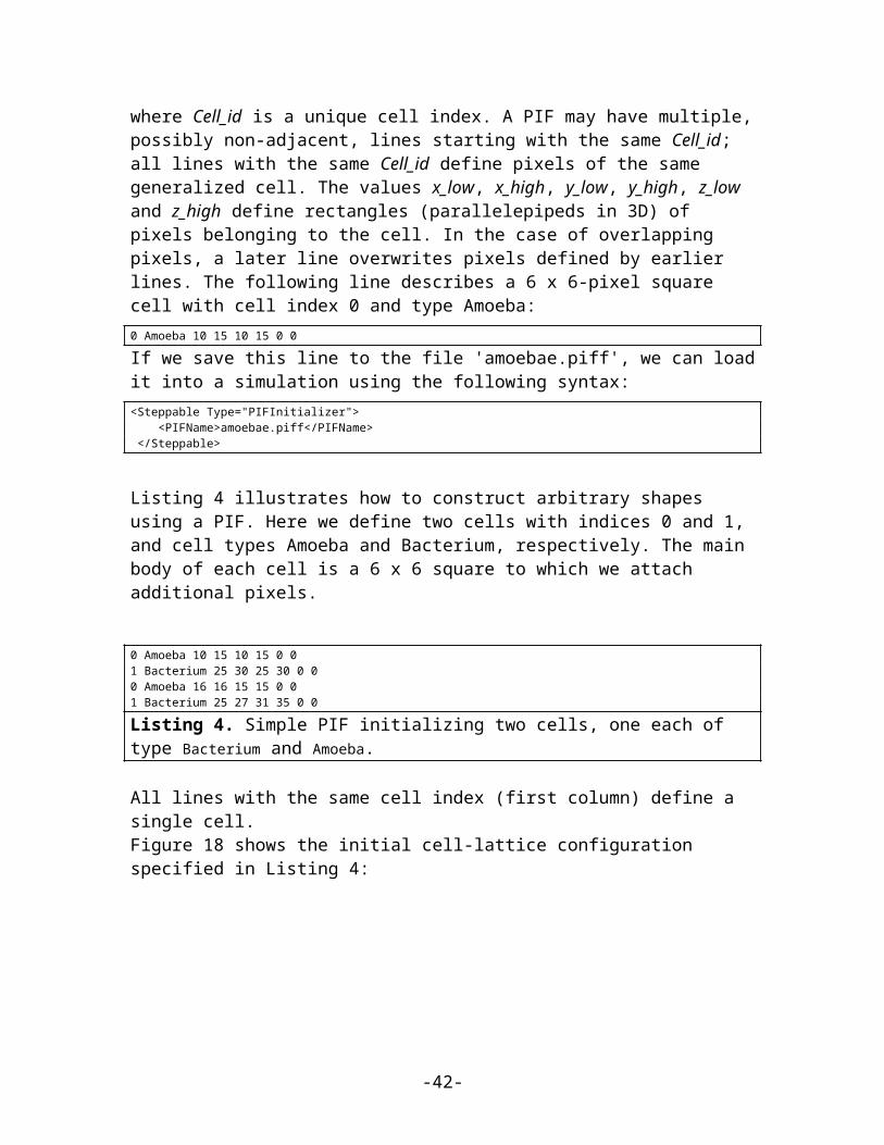
</Plugin> <Plugin Name="Volume"/> <Plugin Name="CenterOfMass"/> <Plugin Name="Contact"> <Energy Type1="Medium" Type2="Medium">0.0</Energy> <Energy Type1="Medium" Type2="Condensing">16.0</Energy> <Energy Type1="Medium" Type2="NonCondensing">16.0</Energy> <Energy Type1="Medium" Type2="DifferentiatedCondensing">16.0</Energy> <Energy Type1="Condensing" Type2="Condensing">2.0</Energy> <Energy Type1="Condensing" Type2="NonCondensing">11.0</Energy> <Energy Type1="Condensing" Type2="DifferentiatedCondensing">2.0</Energy> <Energy Type1="NonCondensing" Type2="NonCondensing">15.0</Energy> <Energy Type1="NonCondensing" Type2="DifferentiatedCondensing">11.0</Energy> <Energy Type1="DifferentiatedCondensing" Type2="DifferentiatedCondensing">2.0</Energy> <NeighborOrder>2</NeighborOrder> </Plugin> <Steppable Type="DiffusionSolverFE"> <DiffusionField> <DiffusionData> <FieldName>FGF</FieldName> <GlobalDiffusionConstant>0.1</GlobalDiffusionConstant> <GlobalDecayConstant>5e-05</GlobalDecayConstant> </DiffusionData> <SecretionData> <Secretion Type="NonCondensing">0.05</Secretion> </SecretionData> <BoundaryConditions> <Plane Axis="X"> <ConstantDerivative PlanePosition="Min" Value="0.0"/> <ConstantDerivative PlanePosition="Max" Value="0.0"/> </Plane> <Plane Axis="Y"> <ConstantDerivative PlanePosition="Min" Value="0.0"/> <ConstantDerivative PlanePosition="Max" Value="0.0"/> </Plane> </BoundaryConditions> </DiffusionField> </Steppable> <Steppable Type="BlobInitializer"> <Region> <Center x="100" y="100" z="0"/> <Radius>40</Radius> <Gap>0</Gap> <Width>5</Width> <Types>Condensing,NonCondensing</Types> </Region> </Steppable></CompuCell3D>
-42-
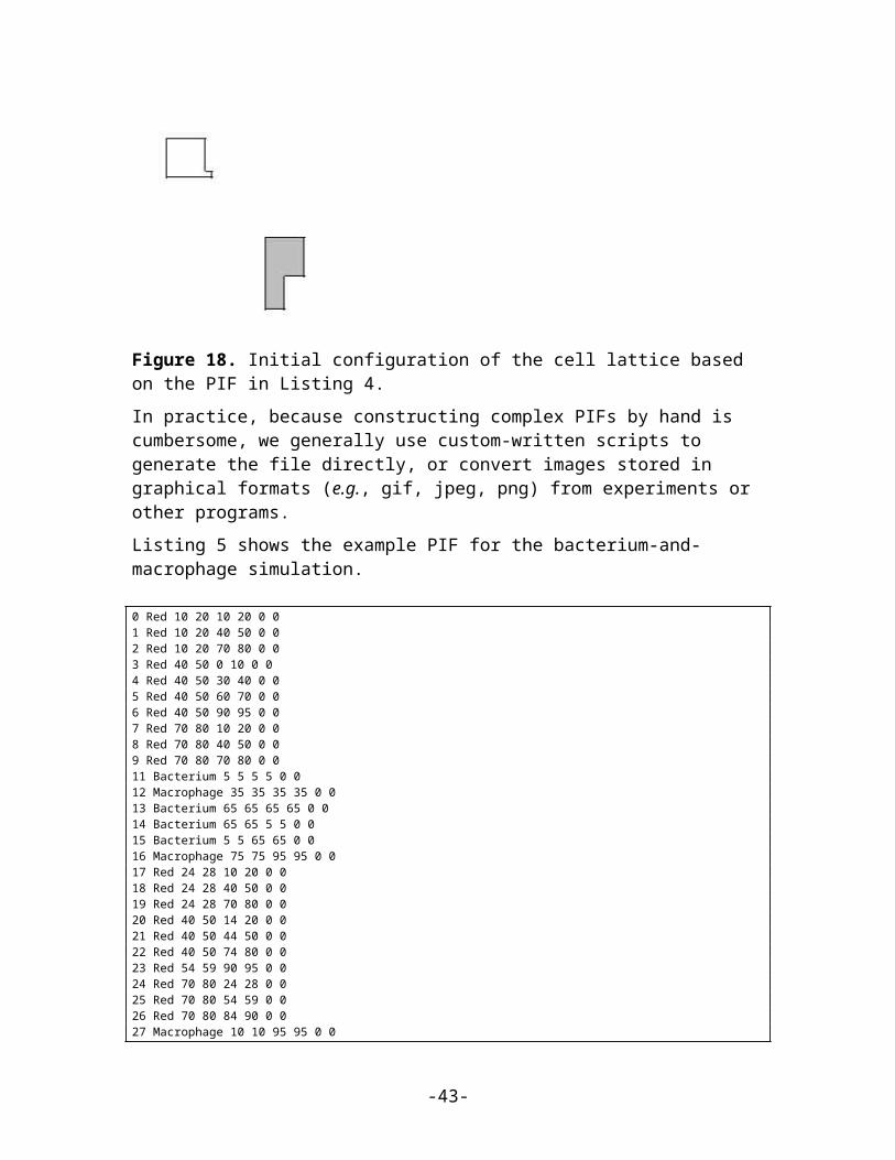
Listing 12. CC3DML code for the diffusing-field-based cell-growth simulation.Changes from the autogenerated template are shown in bold font.
The CC3DML code is a slightly extended version of the cell-sorting code in Listing 1 plus the DiffusionSolverFE discussed in the bacterium-and-macrophage simulation. Note we have specified no-flux boundary conditions even though we could have completely removed this section as no-flux boundary conditions are default choice in CC3D.
The initial cell-lattice does not contain any CondensingDifferentiated cells. These cells appear only as the result of mitosis. We use the VolumeLocalFlex plugin (specifying <Plugin Name=”Volume”/> is sufficient) to allow the target volume to vary individually for each cell, allowing cell growth. We manage the volume-constraint parameters using a Python script. The CenterOfMass plugin provides a reference point in each cell at which we measure the FGF concentration. We then adjust the cell's target volume accordingly.
To build this simulation in CompuCell3D we need to write several Python routines. We need: 1) A steppable, ConstraintInitializerSteppable to initialize the volume-constraint parameters for each cell and to simulate cell growth by periodically increasing Condensing cells’ target volumes in proportion to the FGF concentration at their centroids – we will clal this steppable every 10 MCS as opposed to 100 MCS as generated by Twedit++ . 2) A steppable, MitosisSteppable, that divides cell once it reaches a threshold volume and then adjusts the parameters of the resulting parent and daughter cells. This steppable also appends information about the time and type of cell division to a list attached to each cell. We call this steppable every MCS 3) A steppable, MitosisDataPrinterSteppable, that prints the cell-division information from the lists attached to each cell. We call this steppable every 100 MCS. 4) A class, MitosisData, which MitosisDataPrinterSteppable uses to extract and format the data it prints. 5) A main Python script to call the steppables and the CellsortMitosis plugin appropriately. We store the source code for routines 1)-4) in a separate file called 'cellsort_2D_fieldSteppables.py'.
Listing 13 shows the main Python script for the diffusing-field-based cell-growth simulation.
import sysfrom os import environfrom os import getcwdimport string
sys.path.append(environ["PYTHON_MODULE_PATH"])
import CompuCellSetup
sim,simthread = CompuCellSetup.getCoreSimulationObjects() # add extra attributes herepyAttributeAdder,dictAdder=CompuCellSetup.attachListToCells(sim) CompuCellSetup.initializeSimulationObjects(sim,simthread)# Definitions of additional Python-managed fields go here
-43-
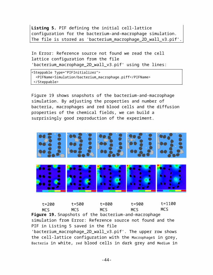
#Add Python steppables heresteppableRegistry=CompuCellSetup.getSteppableRegistry() from cellsort_2D_fieldSteppables import ConstraintInitializerSteppableConstraintInitializerSteppableInstance=ConstraintInitializerSteppable(sim,_frequency=10)steppableRegistry.registerSteppable(ConstraintInitializerSteppableInstance) from cellsort_2D_fieldSteppables import MitosisSteppableMitosisSteppableInstance=MitosisSteppable(sim,_frequency=1)steppableRegistry.registerSteppable(MitosisSteppableInstance) from cellsort_2D_fieldSteppables import MitosisDataPrinterSteppableinstanceOfMitosisDataPrinterSteppable=MitosisDataPrinterSteppable\(_simulator=sim,_frequency=100)steppableRegistry.registerSteppable(instanceOfMitosisDataPrinterSteppable)
CompuCellSetup.mainLoop(sim,simthread,steppableRegistry)
Listing 13. Main Python script for the diffusing-field-based cell-growth simulation. Changes to the template code shown in bold. Attaching Python dictionaries or lists to cells can be accomplished from Twedit++ by calling CC3DPython->CellAttributes->Add Dictionary to Cells on the main Python script.
As compared to ‘vanilla’ CC3D main Python script Listing 13 contains new linepyAttributeAdder,listAdder=CompuCellSetup.attachListToCells(sim)
which instructs the CompuCell3D kernel to attach a Python-defined list to each cell when it creates it. This list serves as a generic container which can store any set of Python objects and hence any set of generalized-cell properties. In the current simulation, we use the list to store objects of the class MitosisData, which records the Monte Carlo Step at which each cell division involving the current cell or its parent, happened, as well as, the cell index and cell type of the parent and daughter cells. We can also attach Python dictionary by using:pyAttributeAdder,listAdder=CompuCellSetup.attachDictionaryToCells(sim)
Since location of this statement is important (you cannot put it just anywhere in the script) it is best to use Twedit++ by calling CC3DPython->CellAttributes->Add Dictionary to Cells on the main Python script.
Moving on to the Python modules, we can see that most of the code looks a lot like other steppable file found in e.g. Listing 10. In addition to steppables, we created one non-steppable MitosisData used to register mitotic events. from PySteppables import *import CompuCellimport sysfrom random import randomfrom PySteppablesExamples import MitosisSteppableBase class ConstraintInitializerSteppable(SteppableBasePy): def __init__(self,_simulator,_frequency=1): SteppableBasePy.__init__(self,_simulator,_frequency) def start(self): for cell in self.cellList: cell.targetVolume=25 cell.lambdaVolume=2.0 def step(self,mcs): field=CompuCell.getConcentrationField(self.simulator,"FGF") comPt=CompuCell.Point3D()
-44-

for cell in self.cellList: if cell.type==self.CONDENSING: #Condensing cell comPt.x=int(round(cell.xCOM)) comPt.y=int(round(cell.yCOM)) comPt.z=int(round(cell.zCOM)) concentration=field.get(comPt) # get concentration at comPt cell.targetVolume+=0.1*concentration # increase cell's target volume #MItosis data has to have base class "object" otherwise if cell will be deleted CC3D may crash due to improper garbage collectionclass MitosisData(object): def __init__(self, _MCS=-1, _parentId=-1, _parentType=-1,\ _offspringId=-1, _offspringType=-1): self.MCS=_MCS self.parentId=_parentId self.parentType=_parentType self.offspringId=_offspringId self.offspringType=_offspringType def __str__(self): return "Mitosis time="+str(self.MCS)+" parentId="+str(self.parentId)+"\ offspringId="+str(self.offspringId)
class MitosisSteppable(MitosisSteppableBase): def __init__(self,_simulator,_frequency=1): MitosisSteppableBase.__init__(self,_simulator, _frequency) def step(self,mcs): cells_to_divide=[] for cell in self.cellList: if cell.volume>50: cells_to_divide.append(cell) for cell in cells_to_divide: self.divideCellRandomOrientation(cell)
def updateAttributes(self): parentCell=self.mitosisSteppable.parentCell childCell=self.mitosisSteppable.childCell parentCell.targetVolume/=2.0 childCell.targetVolume=parentCell.targetVolume childCell.lambdaVolume=parentCell.lambdaVolume
if random()<0.5: childCell.type=parentCell.type else: childCell.type=self.DIFFERENTIATEDCONDENSING #get a reference to lists storing Mitosis data parentCellList=CompuCell.getPyAttrib(parentCell) childCellList=CompuCell.getPyAttrib(childCell)
##will record mitosis data in parent and offspring cells mcs=self.simulator.getStep() mitData=\ MitosisData(mcs,parentCell.id,parentCell.type,childCell.id,childCell.type) parentCellList.append(mitData) childCellList.append(mitData)
class MitosisDataPrinterSteppable(SteppableBasePy): def __init__(self,_simulator,_frequency=10): SteppableBasePy.__init__(self,_simulator,_frequency) def step(self,mcs): for cell in self.cellList: mitDataList=CompuCell.getPyAttrib(cell)
-45-

if len(mitDataList) > 0: print "MITOSIS DATA FOR CELL ID",cell.id for mitData in mitDataList: print mitData
Listing 14. Python steppable code stored in ‘cellsort_2D_fieldSteppables.py’ for the diffusing-field-based cell-growth simulation.
Let us first consider ConstraintInitializerSteppable.The start(self) function executes only once, at the beginning of the simulation. It iterates over each cell (for cell in self.cellList:) and assigns the initial cells’ targetVolume (V t (s )=25 pixels) and lambdaVolume ( ) parameters as the VolumeLocalFlex plugin requires.
The first line of the step(self, mcs) function extracts a reference to the FGF concentration field defined using the DiffusionSolverFE steppable in the CC3DML file (each field created in a CompuCell3D simulation is registered and accessible by both C++ and Python). The function then iterates over every cell in the simulation. If a cell is of cell.type equal to self.CONDENSING, we calculate its centroid, round it to nearest integers:comPt.x=int(round(cell.xCOM))comPt.y=int(round(cell.yCOM))comPt.z=int(round(cell.zCOM))
and retrieve the FGF concentration at that point:concentration=field.get(comPt)
We then increase the target volume of the cell by 0.01 times that concentration:cell.targetVolume+=0.01*concentration
We must include the CenterOfMass plugin in the CC3DML code. Otherwise the centroid (cell.xCOM, cell.yCOM, cell.zCOM) will have the default value (0,0,0). By default Twedit++ includes CenterOfMass plugin in the autogenerated code.The MitosisSteppable divides the mitotic cell into two cells and adjusts both cells' attributes. It also initializes and appends MitosisData objects to the original cell's (self.parentCell) and daughter cell's (self.childCell) attribute lists.
MitosisSteppable inherits the content of the MitosisSteppableBase class. MitosisSteppableBase contains several convenience functions associated with Mitosis even (many of those functions are implemented in C++) and also inherits SteppableBase providing many convenient features of this class. At each MCS (or with user specified frequency) we scan cells and decide which cells are to undergo mitosis: def step(self,mcs): cells_to_divide=[] for cell in self.cellList: if cell.volume>50: cells_to_divide.append(cell) for cell in cells_to_divide: self.divideCellRandomOrientation(cell)
-46-
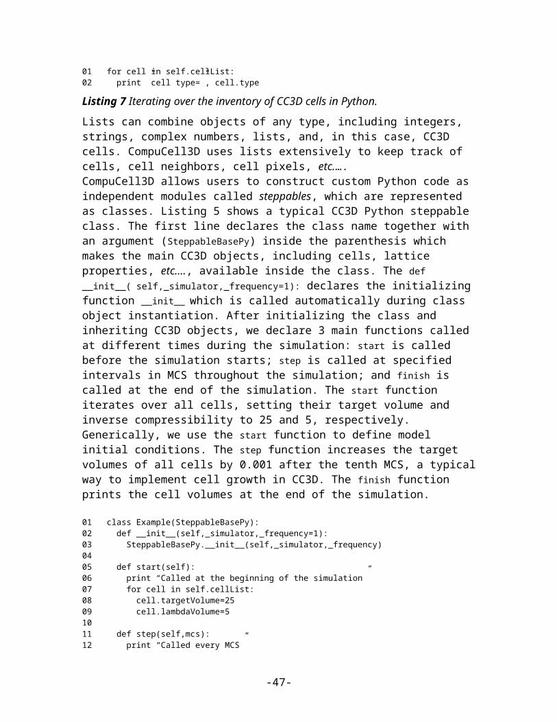
if a cell has volume greater than 50 we attach this cell to the list of cells to be divided (cells_to_divide). Subsequentyl we walk over all the cells stored in cells_to_divide and split them into two cells. Each function from Mitosis Steppable which divides cells calls (immediately after the division takes place) updateAttributes(self)function.Therefore we also need to reimplement the function updateAttributes(self), to define the post-division cells’ parameters. The objects self.childCell and self.parentCell that appear in the function are initialized and managed by MitosisPyPluginBase. In the current simulation, after division we set V t for the parent
and daughter cells to half of the of the parent just prior to cell division. λvol . is left unchanged for the parent cell and the same value is assigned to the daughter cell: self.parentCell.targetVolume=self.parentCell.volume/2.0self.childCell.targetVolume=self.parentCell.targetVolumeself.childCell.lambdaVolume=self.parentCell.lambdaVolume
The cell type of one of the two daughter cells (childCell) is randomly chosen to be either Condensing (i.e., the same as the parent type) or DifferentiatedCondensing: if random()<0.5: childCell.type=parentCell.typeelse: childCell.type=self.DIFFERENTIATEDCONDENSING
Note that we also have to import random() function from random module to ensure that Python finds it:from random import random
The parent cell remains Condensing. We now add a description of this cell division to the lists attached to each cell. First we collect the data in a list called mitData: mcs=self.simulator.getStep() mitData=MitosisData(mcs,self.parentCell.id,self.parentCell.type,\ self.childCell.id,self.childCell.type)
then we access the lists attached to the two cells: parentCellList=CompuCell.getPyAttrib(self.parentCell) childCellList=CompuCell.getPyAttrib(self.childCell)
and append the new mitosis data to these lists: parentCellList.append(mitData) childCellList.append(mitData)
The MitosisData class, which stores the data on the cell division that we append to the cells’ attribute lists after each cell division. In the constructor of MitosisData, we read in the time (in MCS) of the division, along with the parent and daughter cell indices and types. The __str__(self) convenience function returns an ASCII string representation of the time and cell indices only, to allow the Python print command to print out this information.
The MitosisDataPrinterSteppable steppable prints the mitosis data to the user's screen and is shown here mainly to demonstrate that certain plugins inCC3D do not always have to adjust cell parameters – they can access then, print them to the screen or even do something which has little to do with simulation itself (e.g. output file for post processing). To autogenerate steppable for the existing simulation we use Twedit++ CC3D project manager as shown on Figure 23.
-47-

t=200 MCS t=600 MCS t=1200 MCS t=1800 MCS
Figure 23 To autogenerate steppable using Twedit++, right-click on steppable file in the CC3D Project Manager panel and choose Add Steppable… menu optioin which pops-up a simple dialog window.
Within the step(self,mcs) function of the MitosisDataPrinterSteppable, we iterate over each cell and access the Python list attached to the cell (mitDataList=CompuCell.getPyAttrib(cell)). If a given cell has undergone mitosis, then the list will have entries, and thus a nonzero length. If so, we print the MitosisData objects stored in the list: if len(mitDataList) > 0: print "MITOSIS DATA FOR CELL ID",cell.id for mitData in mitDataList: print mitData
Figure 24 and Figure 25 show snapshots of the diffusing-field-based cell-growth simulation. Figure 26 shows a sample screen output of the cell-division history.
Figure 24. Snapshots of the diffusing-field-based cell-growth simulation obtained by running the CC3DML file in Listing 12 in conjunction with the Python file in Listing 13. As the simulation progresses, NonCondensing cells (light gray) secrete diffusing
-48-
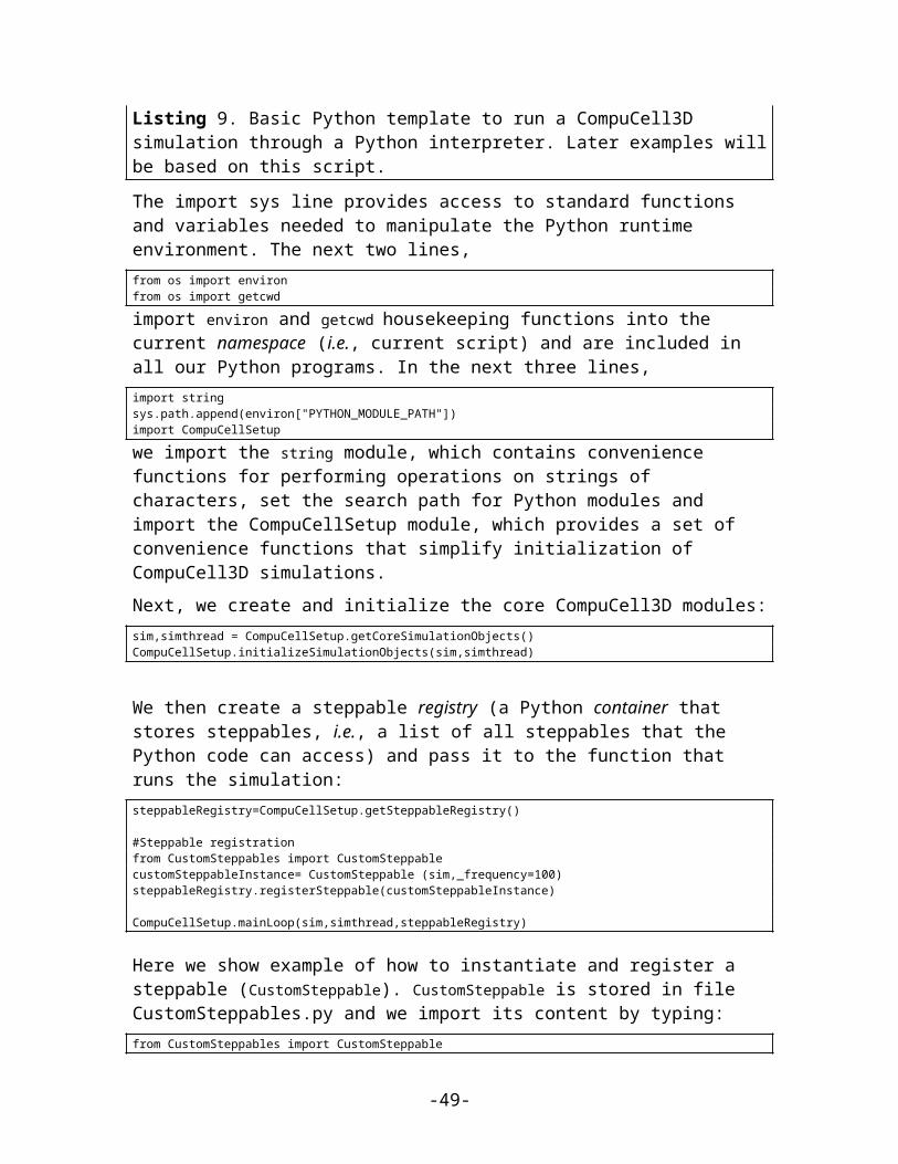
t=200 MCS t=600 MCS t=1200 MCS t=1800 MCS
chemical, FGF, which causes Condensing (dark gray) cells to proliferate. Some Condensing cells differentiate to CondensingDifferentiated (white) cells.
Figure 25. Snapshots of FGF concentration in the diffusing-field-based cell-growth simulation obtained by running the CC3DML file in Listing 12 in conjunction with the Python files in Listing 13, Listing 14, Error: Reference source not found, Error: Reference source not found, Error: Reference source not found. The bars at the bottom of the field images show the concentration scales (blue, low concentration; red, high concentration).
Figure 26. Sample output from the MitosisDataPrinterSteppable steppable in Error: Reference source not found.
-49-

The diffusing-field-based cell-growth simulation includes concepts that extend easily to simulate biological phenomena that involve diffusants, cell growth and mitosis, e.g., limb-bud development (58, 59), tumor growth (5-9) and Drosophila imaginal-disc development.
6.5 Three-Dimensional Vascular Tumor Growth ModelThe development of a primary solid tumor starts from a single cell that proliferates in an inappropriate manner, dividing repeatedly to form a cluster of tumor cells. Nutrient and waste diffusion limits the diameter of such avascular tumor spheroids to about 1 mm. The central region of the growing spheroid becomes necrotic, with a surrounding layer of cells whose hypoxia triggers VEGF-mediated signaling events that initiate tumor neovascularization by promoting growth and extension (neoangiogenesis) of nearby blood vessels. Vascularized tumors are able to grow much larger than avascular spheroids and are more likely to metastasize.Here, we present a simplified 3D model of a generic vascular tumor which can be easily extended to describe specific vascular tumor types and host tissues. We begin with a cluster of proliferating tumor cells, P, and normal vasculature. Initially, tumor cells proliferate as they take up diffusing glucose from the field, GLU, which the pre-existing vasculature supplies (in this model we neglect possible changes in concentration along the blood vessels in the direction of flow and set the secretion parameters uniform over all blood-vessel surfaces). We assume that the tumor cells (both in the initial cluster and later) are always hypoxic and secrete a long-diffusing isoform of VEGF-A, L_VEGF. When GLU drops below a threshold, tumor cells become necrotic, gradually shrink and finally disappear. The initial tumor cluster grows and reaches a maximum diameter characteristic of an avascular tumor spheroid. To reduce execution time in our demonstration, we choose our model parameters so that the maximum spheroid diameter will be about 10 times smaller than in experiment. A few pre-selected neovascular endothelial cells, NV, in the pre-existing vasculature respond both by chemotaxing towards higher concentrations of pro-angiogenic factors and by forming new blood vessels via neoangiogenesis. The tumor-induced vasculature increases the growth rate of the resulting vascularized solid tumor compared to an avascular tumor, allowing the tumor to grow beyond the spheroid’s maximum diameter. Despite our rescaling of the tumor size, the model produces a range of biologically reasonable morphologies that allow study of how tumor-induced angiogenesis affects the growth rate, size and morphology of tumors.We use the basic angiogenesis simulation from the previous section to simulate both pre-existing vasculature and tumor-induced angiogenesis, adding a set of finite-element links between the endothelial cells to model the strong junctions that form between endothelial cells in vivo. We denote the short-diffusing isoform of VEGF-A, S_VEGF. Both endothelial cells and neovascular endothelial cells chemotax up gradients of S_VEGF, but only neovascular endothelial cells chemotax up gradients of L_VEGF. In the Simulation Wizard we name the model TumorVascularization, set the cell- and field-lattice dimensions to 50×50×80, the membrane fluctuation amplitude to 20, the pixel-copy range to 3, number of MCS to 10000 and choose UniformInitializer to produce the initial tumor and vascular cells, since it automatically creates a mixture of the
-50-

cell types. We specify four cell types: P: proliferating tumor cells, N: necrotic cells, EC: endothelial cells and NV: neovascular endothelial cells.On the Chemical Fields page we create the S_VEGF and L_VEGF fields and select FlexibleDiffusionSolverFE for both from the Solver pull-down list. We also check Enable multiple calls of PDE solvers to work around the numerical instabilities of the PDE solvers for large diffusion constants.
Figure 27 Specification of vascular tumor chemical fields in Simulation Wizard.
On the Cell Behavior and Properties page we select both the Contact and FocalPointPlasticity modules from the Adhesion group, and add Chemotaxis, Growth and Mitosis, Volume Constraint and Global Connectivity by checking the appropriate boxes. We also track the Center-of-Mass (to access field concentrations) and Cell Neighbors (to implement contact-inhibited growth). Unlike in our angiogenesis simulation, we will implement secretion as a part of the FlexibleDiffusionSolverFE syntax.
Figure 28 Specification of vascular tumor cell behaviors in Simulation Wizard.
In the Chemotaxis page, for each cell-type/chemical-field pair we click the Add Entry button to add the relevant chemotaxis information, e.g. we select S_VEGF from the Field pull-down list and EC and NV from the cell-type list and set Lambda to 5000. To enable contact inhibition of EC and NV chemotaxis we select Medium from the pull-down menu next to the Chemotax Towards button and click the button to add Medium to the list. We repeat this process for the T and N cell types, so that NV cells chemotax up gradients of L_VEGF. We then proceed to the final Simulation Wizard page.
-51-
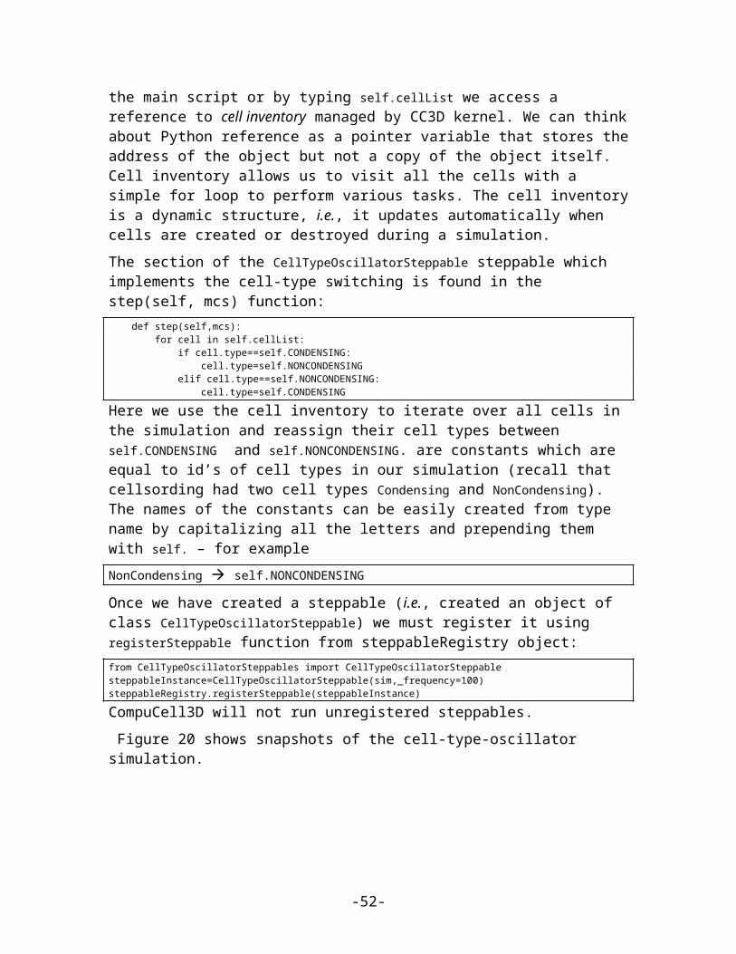
Figure 29 Specification of vascular tumor chemotaxis properties in Simulation Wizard.
Twedit++ generates 3 simulation files – a CC3DML file specifying the energy terms, diffusion solvers and initial cell layout, a main Python file which loads the CC3DMLfile, sets up the CompuCell environment and executes the Python steppables and a Python steppables file. The main Python file is typically constructed by modifying the standard template in Listing 6. Lines 1-12 set up the CC3D simulation environment and load the simulation. Lines 14-20 create instances of two steppables – MitosisSteppable and VolumeParamSteppable – and register them with the CC3D kernel. Line 22 starts the main CC3D loop, which executes Monte Carlo Steps and periodically calls the steppables.
01 import sys02 from os import environ03 import string04 sys.path.append(environ["PYTHON_MODULE_PATH"])05 06 import CompuCellSetup07 sim,simthread = CompuCellSetup.getCoreSimulationObjects()08 CompuCellSetup.initializeSimulationObjects(sim,simthread)09 import CompuCell10 11 from PySteppables import SteppableRegistry12 steppableRegistry=SteppableRegistry()13 14 from VascularTumorSteppables import MitosisSteppable15 mitosisSteppable=MitosisSteppable(sim,1)16 steppableRegistry.registerSteppable(mitosisSteppable)17 18 from VascularTumorSteppables import VolumeParamSteppable19 volumeParamSteppable=VolumeParamSteppable(sim,1)20 steppableRegistry.registerSteppable(volumeParamSteppable)21 22 CompuCellSetup.mainLoop(sim,simthread,steppableRegistry)
Listing 15 The Main Python script initializes the vascular tumor simulation and runs the main simulation loop.
Next, we edit the draft autogenerated simulation CC3DML file in Listing 7. 01 <CompuCell3D>02 <Potts>03 <Dimensions x="50" y="50" z="80"/>04 <Steps>100000</Steps>05 <Temperature>20</Temperature>06 <Boundary_x>Periodic</Boundary_x>
-52-
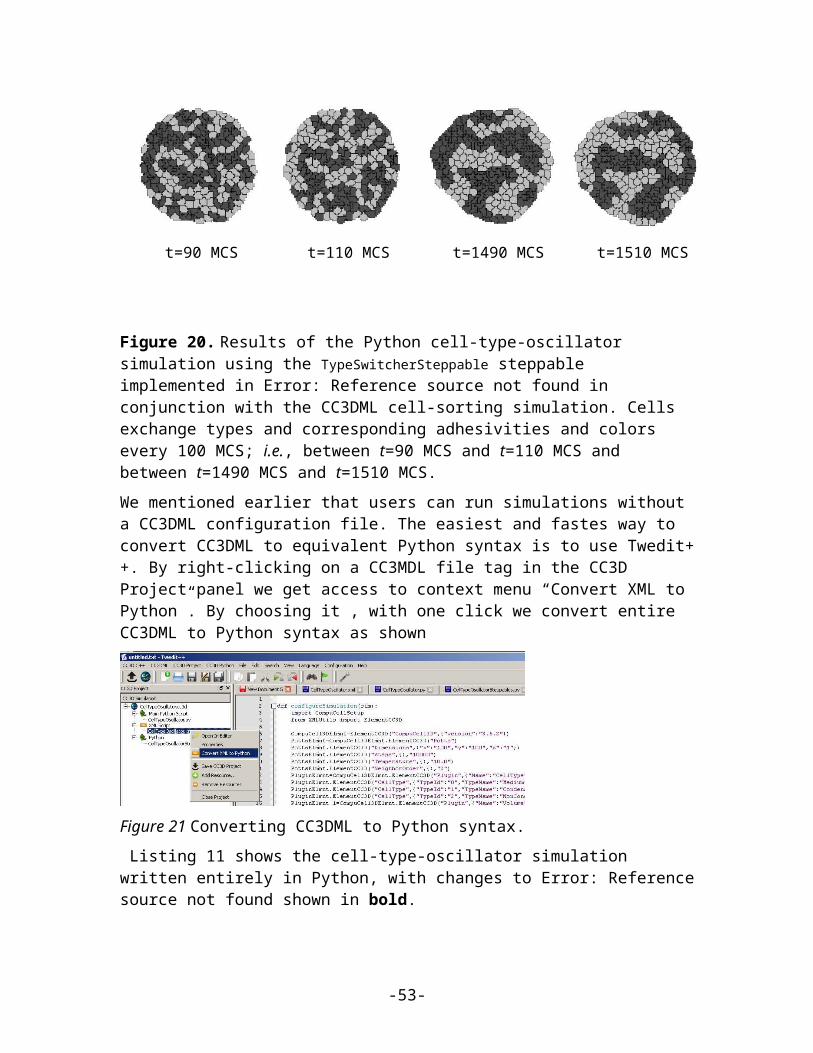
07 <Boundary_y>Periodic</Boundary_y>08 <Boundary_z>Periodic</Boundary_z>09 <RandomSeed>313</RandomSeed>10 <NeighborOrder>3</NeighborOrder>11 </Potts>12 13 <Plugin Name="CellType">14 <CellType TypeName="Medium" TypeId="0"/>15 <CellType TypeName="P" TypeId="1"/>16 <CellType TypeName="N" TypeId="2"/>17 <CellType TypeName="EC" TypeId="3"/> 18 <CellType TypeName="NV" TypeId="4"/> 19 </Plugin>20 21 <Plugin Name="Chemotaxis">22 <ChemicalField Source="FlexibleDiffusionSolverFE" Name="S_VEGF">23 <ChemotaxisByType Type="NV" Lambda="5000" ChemotactTowards="Medium,P,N"/>24 </ChemicalField>25 <ChemicalField Source="FlexibleDiffusionSolverFE" Name="L_VEGF">26 <ChemotaxisByType Type="NV" Lambda="1000" ChemotactTowards="Medium,P,N" SaturationCoef="0.05"/>27 </ChemicalField>28 <ChemicalField Source="FlexibleDiffusionSolverFE" Name="S_VEGF">29 <ChemotaxisByType Type="EC" Lambda="5000" ChemotactTowards="Medium,P,N"/>30 </ChemicalField>31 </Plugin>32 33 <Plugin Name="CenterOfMass"/>34 <Plugin Name="NeighborTracker"/>35 36 <Plugin Name="Contact">37 <Energy Type1="Medium" Type2="Medium">0</Energy>38 <Energy Type1="P" Type2="Medium">10</Energy>39 <Energy Type1="P" Type2="P">8</Energy>40 <Energy Type1="N" Type2="Medium">15</Energy>41 <Energy Type1="N" Type2="P">8</Energy>42 <Energy Type1="N" Type2="N">3</Energy>43 <Energy Type1="EC" Type2="Medium">12</Energy>44 <Energy Type1="EC" Type2="P">30</Energy>45 <Energy Type1="EC" Type2="N">30</Energy>46 <Energy Type1="EC" Type2="EC">5</Energy>47 <Energy Type1="NV" Type2="Medium">12</Energy>48 <Energy Type1="NV" Type2="P">30</Energy>49 <Energy Type1="NV" Type2="N">30</Energy>50 <Energy Type1="NV" Type2="EC">5</Energy>51 <Energy Type1="NV" Type2="NV">5</Energy>52 <NeighborOrder>4</NeighborOrder>53 </Plugin>54 55 <Plugin Name="VolumeLocalFlex"/>56 57 <Plugin Name="FocalPointPlasticity">58 <Parameters Type1="EC" Type2="NV">59 <Lambda>50.0</Lambda>60 <ActivationEnergy>-100.0</ActivationEnergy>61 <TargetDistance>5.0</TargetDistance>62 <MaxDistance>15.0</MaxDistance>63 <MaxNumberOfJunctions>2</MaxNumberOfJunctions>64 </Parameters>65 <Parameters Type1="EC" Type2="EC">66 <Lambda>400.0</Lambda>67 <ActivationEnergy>-100.0</ActivationEnergy>68 <TargetDistance>5.0</TargetDistance>
-53-

69 <MaxDistance>15.0</MaxDistance>70 <MaxNumberOfJunctions>3</MaxNumberOfJunctions>71 </Parameters>72 <Parameters Type1="NV" Type2="NV">73 <Lambda>20.0</Lambda>74 <ActivationEnergy>-100.0</ActivationEnergy>75 <TargetDistance>5.0</TargetDistance>76 <MaxDistance>10.0</MaxDistance>77 <MaxNumberOfJunctions>2</MaxNumberOfJunctions>78 </Parameters>79 <NeighborOrder>1</NeighborOrder>80 </Plugin>81 82 <Plugin Name="ConnectivityGlobal">83 <Penalty Type="NV">10000</Penalty>84 <Penalty Type="EC">10000</Penalty>85 </Plugin>86 87 <Plugin Name="PDESolverCaller">88 <CallPDE PDESolverName="FlexibleDiffusionSolverFE" ExtraTimesPerMC="9"/>89 </Plugin>90 91 <Steppable Type="FlexibleDiffusionSolverFE">92 <!--endothelial-derived short diffusing VEGF isoform-->93 <DiffusionField>94 <DiffusionData>95 <FieldName>S_VEGF</FieldName>96 <ConcentrationFileName></ConcentrationFileName>97 <DiffusionConstant>0.016</DiffusionConstant>98 <DecayConstant>0.0016</DecayConstant>99 <DoNotDecayIn>EC</DoNotDecayIn>100 <DoNotDecayIn>NV</DoNotDecayIn>101 </DiffusionData>102 <SecretionData>103 <Secretion Type="NV">0.0013</Secretion>104 <Secretion Type="EC">0.0013</Secretion>105 </SecretionData>106 </DiffusionField>107 108 <!--tumor-derived long diffusing VEGF isoform-->109 <DiffusionField>110 <DiffusionData>111 <FieldName>L_VEGF</FieldName>112 <DiffusionConstant>0.16</DiffusionConstant>113 <DecayConstant>0.0016</DecayConstant>114 </DiffusionData>115 <SecretionData>116 <Secretion Type="P">0.001</Secretion>117 <Uptake Type="NV" MaxUptake="0.05" RelativeUptakeRate="0.5"/>118 <Uptake Type="EC" MaxUptake="0.05" RelativeUptakeRate="0.5"/>119 </SecretionData>120 </DiffusionField>121 122 <DiffusionField>123 <DiffusionData>124 <FieldName>GLU</FieldName>125 <ConcentrationFileName>GLU_300.dat</ConcentrationFileName>126 <DiffusionConstant>0.16</DiffusionConstant>127 </DiffusionData>128 <SecretionData>129 <Secretion Type="NV">0.4</Secretion>130 <Secretion Type="EC">0.8</Secretion>131 <Uptake Type="Medium" MaxUptake="0.0064" RelativeUptakeRate="0.1"/>
-54-

132 <Uptake Type="P" MaxUptake="0.1" RelativeUptakeRate="0.1"/>133 </SecretionData>134 </DiffusionField>135 </Steppable>136 137 <Steppable Type="UniformInitializer">138 <Region>139 <BoxMin x="0" y="24" z="16"/>140 <BoxMax x="50" y="28" z="20"/>141 <Width>4</Width>142 <Types>EC</Types>143 </Region>144 <Region>145 <BoxMin y="0" x="24" z="16"/>146 <BoxMax y="50" x="28" z="20"/>147 <Width>4</Width>148 <Types>EC</Types>149 </Region>150 <Region>151 <BoxMin x="10" y="24" z="16"/>152 <BoxMax x="50" y="28" z="20"/>153 <Width>4</Width>154 <Gap>25</Gap>155 <Types>NV</Types>156 </Region>157 <Region>158 <BoxMin y="8" x="24" z="16"/>159 <BoxMax y="50" x="28" z="20"/>160 <Width>4</Width>161 <Gap>25</Gap>162 <Types>NV</Types>163 </Region>164 <Region>165 <BoxMin x="26" y="26" z="40"/>166 <BoxMax x="34" y="34" z="48"/>167 <Width>2</Width>168 <Types>P</Types>169 </Region>170 </Steppable>171 172 </CompuCell3D>
Listing 16 CC3DML specification of the vascular tumor model’s initial cell layout, PDE solvers and key cellular behaviors.
In Listing 7, in the Contact plugin (lines 36-53), we set JMM=0, JEM=12 and JEE=5 (M: Medium, E: EC) and the NeighborOrder to 4. The FocalPointPlasticity plugin (lines 57-80) represents adhesion junctions by mechanically connecting the centers-of-mass of cells using a breakable linear spring (see Shirinifard et al., 2009). EC-EC links are stronger than EC-NV links, which are, in turn, stronger than NV-NV links (see the CC3D manual for details). Since, the Simulation Wizard creates code to implement links between all cell-type pairs in the model, we must delete most of them, keeping only the links between EC-EC, EC-NV and NV-NV cell types.
We assume that L_VEGF diffuses 10 times faster than S_VEGF, so =0.42 µm2/sec (1.6 voxel2/MCS). This large diffusion constant would make the diffusion solver unstable. Therefore in the CC3DML file (Listing 7, lines 108-114), we set the values of the <DiffusionConstant> and <DecayConstant> tags of the L_VEGF field to 0.16 and
-55-

0.0016 respectively and use 9 extra calls per MCS to achieve a diffusion constant equivalent to 1.6 (lines 87-89). We instruct P cells to secrete (line 116) into the L_VEGF field at a rate of 0.001 (3.85 pg (cell h)-1=0.001 pg (voxel MCS)-1). Both EC and NV absorb L_VEGF. To simulate this uptake, we use the <SecretionData> tag pair (lines 117-118).Since the same diffusion solver will be called 10 times per MCS to solve S_VEGF, we must reduce the diffusion constant of S_VEGF by a factor of 10, setting the <DiffusionConstant> and <DecayConstant> tags of S_VEGF field to 0.016 and 0.0016 respectively. To prevent S_VEGF decay inside EC and NV cells we add <DoNotDecayIn>EC</DoNotDecayIn> and <DoNotDecayIn>NV</DoNotDecayIn> inside the <DiffusionData> tag pair (lines 99-100). We define S_VEGF to be secreted (lines 102-105) by both the EC and NV cells types at a rate of 0.013 per voxel per MCS (50 pg (cell h)-1 = 0.013 pg (voxel MCS)-1, compare to Leith and Michelson 1995). The experimental glucose diffusion constant is about 600 µm2/sec. We convert the glucose diffusion constant by multiplying by appropriate spatial and temporal conversion factors: 600 µm2/sec×(voxel/4 µm)2×(60 sec/MCS)=2250 voxel2/MCS. To keep our simulation times short for the example we use a simulated glucose diffusion constant 1500 smaller, resulting in much steeper glucose gradients and smaller maximum tumor diameters. We could use the steady-state diffusion solver for the glucose field to be more realistic. Experimental GLU uptake by P cells is ~ 0.3 µmol/g/min. We assume that stromal cells (represented here without individual cell boundaries by Medium) take up GLU at a slower rate of 0.1 µmol/g/min. A gram of tumor tissue has about 108 tumor cells, so the glucose uptake per tumor cell is 0.003 pmol/MCS/cell or about 0.1 fmol/MCS/voxel. We assume that (at homeostasis) the pre-existing vasculature supplies all the required GLU to Medium, which has a total mass of 1.28×10⁻⁵ grams and consumes GLU at a rate of 0.1 fmol/MCS/voxel, so the total GLU uptake (in the absence of a tumor) is 1.28 pmol/MCS. For this glucose to be supplied by 24 EC cells, their GLU secretion rate must be 0.8 fmol/MCS/voxel. We distribute the total GLU uptake (in the absence of a tumor) over all the Medium voxels, so the uptake rate is ~ 1.28 pmol/MCS/(~20000 Medium voxels)=6.4×10⁻³ fmol/MCS/voxel.We specify the uptake of GLU by Medium and P cells in lines 131-132 and instruct NV and EC cells to secrete GLU at the rate 0.4 and 0.8 pg (voxel MCS)-1 respectively (lines 129-130)We use UniformInitializer (lines 137-170) to initialize the tumor-cell cluster and two crossing vascular cords. We also add two NV cells to each vascular cord, 25 pixels apart.
01 from PySteppables import *02 from PySteppablesExamples import MitosisSteppableBase03 import CompuCell04 import sys05 from random import uniform06 import math07 08 class VolumeParamSteppable(SteppableBasePy):09 def __init__(self,_simulator,_frequency=1):10 SteppableBasePy.__init__(self, _simulator,_frequency)11 self.fieldL_VEGF = CompuCell.getConcentrationField('L_VEGF') 12 self.fieldGLU = CompuCell.getConcentrationField('GLU')13
-56-
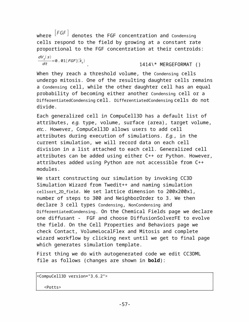
14 def start(self):15 for cell in self.cellList:16 if (cell.type>=3):17 cell.targetVolume=64.0+10.018 cell.lambdaVolume=20.019 else:20 cell.targetVolume=32.021 cell.lambdaVolume=20.022 23 def step(self,mcs):24 pt=CompuCell.Point3D() 25 for cell in self.cellList:26 if (cell.type==4): #Neovascular cells (NV)27 totalArea=028 pt.x=int(round(cell.xCOM))29 pt.y=int(round(cell.yCOM))30 pt.z=int(round(cell.zCOM))31 VEGFconc=self.fieldL_VEGF.get(pt)32 cellNeighborList=self.getNeighborList(cell)33 for nsd in cellNeighborList:34 if (nsd.neighborAddress and nsd.neighborAddress.type>=3):35 totalArea+=nsd.commonSurfaceArea 36 if (totalArea<45):37 cell.targetVolume+=2.0*VEGFconc/(0.01+VEGFconc) 38 if (cell.type==1): #Proliferating Cells39 pt.x=int(round(cell.xCOM))40 pt.y=int(round(cell.yCOM))41 pt.z=int(round(cell.zCOM))42 gluConc=self.fieldGLU.get(pt)43 #Proliferating Cells become Necrotic when gluConc is low44 if (gluConc<0.001 and mcs>1000):45 cell.type=246 else:47 cell.targetVolume+=0.022*gluConc/(0.05+gluConc)48 if cell.type==2: #Necrotic Cells49 cell.targetVolume-=0.150 if cell.targetVolume<0.0:51 cell.targetVolume=0.0 52 53 54 class MitosisSteppable(MitosisSteppableBase):55 def __init__(self,_simulator,_frequency=1):56 MitosisSteppableBase.__init__(self,_simulator,_frequency)57 58 def step(self,mcs):59 cells_to_divide=[]60 for cell in self.cellList:61 if (cell.type==1 and cell.volume>64):62 cells_to_divide.append(cell)63 if (cell.type==4 and cell.volume>128):64 cells_to_divide.append(cell)65 for cell in cells_to_divide:66 self.divideCellRandomOrientation(cell)67 68 def updateAttributes(self):69 parentCell=self.mitosisSteppable.parentCell70 childCell=self.mitosisSteppable.childCell71 parentCell.targetVolume=parentCell.targetVolume/272 parentCell.lambdaVolume=parentCell.lambdaVolume73 childCell.type=parentCell.type74 childCell.targetVolume=parentCell.targetVolume75 childCell.lambdaVolume=parentCell.lambdaVolume
-57-

Listing 17 Vascular tumor model Python steppables. The VolumeParametersSteppable adjusts the properties of the cells in response to simulation events and the MitosisSteppable implements cell division.
In the Python Steppable script in Listing 8, we set the initial target volume of both EC and NV cells to 74 (64+10) voxels and the initial target volume of tumor cells to 32 voxels
(lines 14-21). All λvol are 20.0. To model tumor cell growth, we increase the tumor cells’ target volumes (lines 38-47)
according to:
, (1)
where is the GLU concentration at the cell’s center-of-mass of and is the concentration at which the growth rate is half its maximum. We assume that the fastest
cell cycle time is 24 hours, so is 32 voxels/24 hours = 0.022 voxel/MCS.To account for contact-inhibited growth of NV cells, when their common surface area
with other EC and NV cells is less than a threshold, we increase their target volume according to:
, (2)
where is the concentration of L_VEGF at the cell’s center-of-mass,
is the concentration at which the growth rate is half its maximum and is the maximum growth rate for NV cells. We calculate the common surface area between each NV cell and its neighboring NV or EC cells in lines 32-35. If the common surface area is smaller than 45, then we increase its target volume (lines 36-37). When the volume of NV and P cells reaches a doubling volume (here, twice their initial target volumes), we divide them along a random axis, as shown in the MitosisSteppable (Listing 8, lines 54-75).
-58-
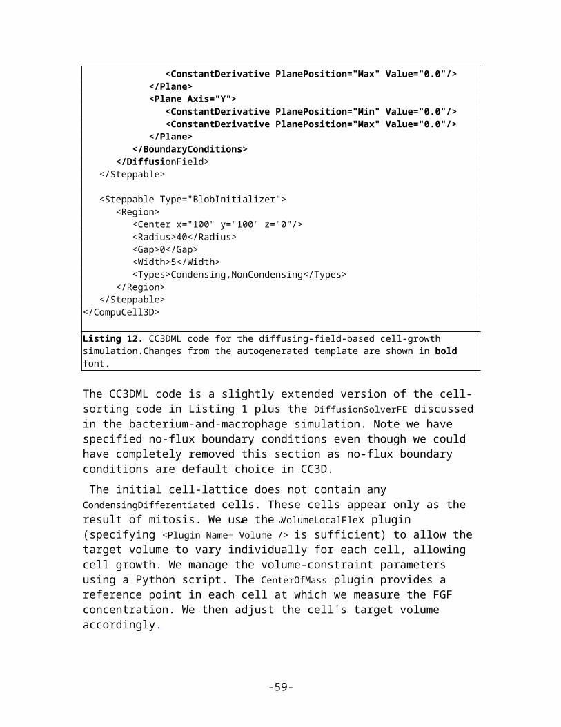
Figure 30 3D snapshots of the vascular tumor simulation taken at: A) 0 MCS , B) 500 MCS, C) 2000 MCS and D) 5000 MCS. Red and Yellow cells represent endothelial cells and neovascular endothelial cells, respectively.
With this simple model we can easily explore the effects of changes in cell adhesion, nutrient availability, cell motility, sensitivity to starvation or dosing with chemotherapeutics or antiangiogenics on the growth and morphology of the simulated tumor.
6.6 Subcellular Simulations Using BionetSolverWhile our vascular tumor model showed how to change cell-level parameters like target volume, we have not yet linked macroscopic cell behaviors to intracellular molecular concentrations. Signaling, regulatory and metabolic pathways all steer the behaviors of biological cells by modulating their biochemical machinery. CC3D allows us to add and solve subcellular reaction-kinetic pathway models inside each generalized cell, specified using the SBML format (Hucka et al. 2003), and to use such models (e.g. of their levels of gene expression) to control cell-level behaviors like adhesion or growth. We can use the same SBML framework to implement classic physics-based pharmacokinetic (PBPK) models of supercellular chemical flows between organs or tissues. The ability to explicitly model such subcellular and supercellular pathways adds greatly to the range of hypotheses CC3D models can represent and test. In addition, the original formulation of SBML primarily focused on the behaviors of biochemical networks within a single cell, while real signaling networks often involve the coupling of networks between cells. BionetSolver supports such coupling, allowing exploration of the very complex feedback resulting from intercell interactions linking intracellular networks in an environment where the couplings change continuously due to cell growth, cell movement and changes in cell properties. As an example of such interaction between signaling networks and cell behaviors, we will develop a multicellular implementation of Delta-Notch mutual inhibitory coupling. In this juxtacrine signaling process, a cell’s level of membrane-bound Delta depends on its intracellular level of activated Notch, which in turn depends on the average level of membrane-bound Delta of its neighbors. In such a situation, the Delta-Notch dynamics of the cells in a tissue sheet will depend on the rate of cell rearrangement and the fluctuations it induces. While the example does not explore the richness due to the coupling of subcellular networks with intercellular networks and cell behaviors, it already shows how different such behaviors can be from those of their non-spatial simplifications. We begin with the Ordinary Differential Equation (ODE) Delta-Notch patterning model of Collier et al. 1996 in which juxtacrine signaling controls the internal levels of the cells’ Delta and Notch proteins. The base model neglects the complexity of the interaction due to changing spatial relationships in a real tissue:
dDdt =v⋅( 1
1+b⋅N h−D), (3)
dNdt
= D k
a+Dk −N, (4)
-59-

where D and N are the concentrations of activated Delta and Notch proteins inside a cell, D is the average concentration of activated Delta protein at the surface of the cell’s neighbors, a and b are saturation constants, h and k are Hill coefficients, and v is a constant that gives the relative lifetimes of Delta and Notch proteins.
Figure 31 Diagram of Delta-Notch feedback regulation between and within cells.
Notch activity increases with the levels of Delta in neighboring cells, while Delta activity decreases with increasing Notch activity inside a cell (Figure 31). When the parameters in the ODE model are chosen correctly, each cell assumes one of two exclusive states: a primary fate, in which the cell has a high level of Delta and a low level of Notch activity, and a secondary fate, in which the cell has a low level of Delta and a high level of Notch. To build this model in CC3D, we assign a separate copy of the ODE model [1-2] to each cell and allow each cell to see the Delta concentrations of its neighbors. We use CC3D’s BionetSolver library to manage and solve the ODEs, which are stored using the SBML standard. The three files that specify the Delta-Notch model are included in the CompuCell3D installation and can be found at <CC3D-installation-dir>/DemosBionetSolver/DeltaNotch: the main Python file (DeltaNotch.py) sets the parameters and initial conditions; the Python steppable file (DeltaNotch_Step.py) calls the subcellular models; and the SBML file (DN_Collier.sbml) contains the description of the ODE model. The first two files can be generated and edited using Twedit++, the last can be generated and edited using an SBML editor like Jarnac or JDesigner (both are open source). Listing 9 shows the SBML file viewed using Jarnac (www.sys-bio.org).
01 p = defn cell02 vol compartment;03 var D, N;04 ext Davg, X;05 $X -> N; pow(Davg,k)/(a+pow(Davg,k))-N;06 $X -> D; v*(1/(1+b*pow(N,h))-D);07 end;08 09 p.compartment = 1;10 p.Davg = 0.4;11 p.X = 0;12 p.D = 0.5;13 p.N = 0.5;14 p.k = 2;15 p.a = 0.01;16 p.v = 1;17 p.b = 100;
-60-

18 p.h = 2;
Listing 18 Jarnac specification of the Delta-Notch coupling model in Figure 31.
The main Python file (DeltaNotch.py) includes lines to define a steppable class (DeltaNotchClass) to include the ODE model and its interactions with the CC3D generalized cells (Listing 10).
01 from DeltaNotch_Step import DeltaNotchClass02 deltaNotchClass=DeltaNotchClass(_simulator=sim,_frequency=1)03 steppableRegistry.registerSteppable(deltaNotchClass)
Listing 19 Registering DeltaNotchClass in the main Python script, DeltaNotch.py in the Delta-Notch model.
The Python steppable file (Listing 11, DeltaNotch_Step.py) imports the BionetSolver library (line 1), then defines the class and initializes the solver inside it (lines 2-5).
01 import bionetAPI02 class DeltaNotchClass(SteppableBasePy):03 def __init__(self,_simulator,_frequency):04 SteppableBasePy.__init__(self,_simulator,_frequency)05 bionetAPI.initializeBionetworkManager(self.simulator)06 07 def start(self):08 #Loading model09 Name = "DeltaNotch"10 Key = "DN"11 Path = os.getcwd()+"\DemosBionetSolver\DeltaNotch\DN_Collier.sbml"12 IntegrationStep = 0.213 bionetAPI.loadSBMLModel(Name, Path, Key, IntegrationStep)14 15 bionetAPI.addSBMLModelToTemplateLibrary(sbmlModelName,"TypeA")16 bionetAPI.initializeBionetworks()17 18 import random 19 for cell in self.cellList:20 D = random.uniform(0.9,1.0)21 N = random.uniform(0.9,1.0)22 bionetAPI.setBionetworkValue("DN_D",D,cell.id)23 bionetAPI.setBionetworkValue("DN_N",N,cell.id)24 cellDict=CompuCell.getPyAttrib(cell)25 cellDict["D"]=D26 cellDict["N"]=N
Listing 20 Implementation of the __init__ and start functions of the DeltaNotchClass in the Delta-Notch model.
The first lines in the start function (Listing 11, lines 9-12) specify the name of the model, its nickname (for easier reference), the path to the location where the SBML model is stored, and the time-step of the ODE integrator, which fixes the relation between MCS and the time units of the ODE model (here, 1 MCS corresponds to 0.2 ODE model time units). In line 13 we use the defined names, path and time-step parameter to load the SBML model.Listing 11, line 15 associates the subcellular model with the CC3D cells, creating an instance of the ODE solver (described by the SBML model) for each cell of type TypeA. Line 16 initializes the loaded subcellular models.
-61-

To set the initial levels of Delta (D) and Notch (N) in each cell, we visit all cells and assign random initial concentrations between 0.9 and 1.0 (Listing 11, lines 18-26). Line 18 imports the intrinsic Python random number generator. Lines 23-24 pass these values to the subcellular models in each cell. The first argument specifies the ODE model parameter to change with a string containing the nickname of the model, here DN, followed by an underscore and the name of the parameter as defined in the SBML file. The second argument specifies the value to assign to the parameter, and the last argument specifies the cell id. For visualization, we store the values of D and N in a dictionary attached to each cell (lines 25-26).
Figure 32 Initial Notch (left) and Delta (right) concentrations in the Delta-Notch model.
Listing 12 defines a step function of the class, which is called every MCS, to read the Delta concentrations of each cell’s neighbors to determine the value of D (the average Delta concentration around the cell). The first three lines in listing 12 iterate over all cells. Inside the loop, we first set the variables D and nn to zero. They will store the total Delta concentration of the cell’s neighbors and the number of neighbors, respectively. Next we get a list of the cell’s neighbors and iterate over them. Line 9 reads the Delta concentration of each neighbor (the first argument is the name of the parameter and the second is the id of the neighboring cell) summing the total Delta and counting the number of neighbors. Note the += syntax (e.g., nn+=1 is equivalent to nn=nn+1). Lines 3 and 7 skip Medium (Medium has a value 0, so if (Medium) is false).
01 def step(self,mcs):02 for cell in self.cellList:03 if cell:04 D=0.0; nn=005 cellNeighborList=self.getCellNeighbors(cell)06 for nsd in cellNeighborList:07 if nsd:08 nn+=109 D+=bionetAPI.getBionetworkValue("DN_D",nsd.neighborAddress.id)10 if (nn>0):11 D=D/nn12 bionetAPI.setBionetworkValue("DN_Davg",D,cell.id)13 cellDict=CompuCell.getPyAttrib(cell)14 cellDict["D"]=D
-62-
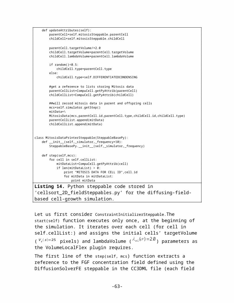
15 cellDict["N"]=bionetAPI.getBionetworkValue("DN_N",cell.id) 16 bionetAPI.timestepBionetworks()
Listing 21 Implementation of a step function to calculate D in the DeltaNotchClass in the Delta-Notch model.
After looping over the cell’s neighbors, we set its new value of the variableD , which in the SBML code has the name Davg, to the average neighboring Delta (D) concentration, ensuing that the denominator, nn, is not zero (Listing 12, lines 10-12). The remaining lines (Listing 12, lines 13-15) access the cell dictionary and store the cell’s current Delta and Notch concentrations. Line 16 then calls BionetSolver and tell it to integrate the ODE model with the new parameters for one integration step (0.2 time units in this case). Figure 33 shows a typical cell configurations and states for the simulation. The random initial values gradually converge to a pattern with cells with low levels of Notch (primary fate) surrounded by cells with high levels of Notch (secondary fate).
Figure 33 Dynamics of the Notch concentrations of cells in the Delta-Notch model. Snapshots taken at 10, 100, 300, 400, 450 and 600 MCS.
Listing 13 lines 2-4 define two new visualization fields in the main Python file (DeltaNotch.py) to visualize the Delta and Notch concentrations in CompuCell Player. To fill the fields with the Delta and Notch concentrations we call the steppable class, ExtraFields (Listing 13, lines 6-9). This code is very similar to our previous steppable calls, with the exception of line 8, which uses the function setScalarFields()to reference the visualization Fields.
01 #Create extra player fields here or add attributes02 dim=sim.getPotts().getCellFieldG().getDim()03 DeltaField=simthread.createScalarFieldCellLevelPy("Delta")04 NotchField=simthread.createScalarFieldCellLevelPy("Notch")05 06 from DeltaNotch_Step import ExtraFields07 extraFields=ExtraFields(_simulator=sim,_frequency=5)08 extraFields.setScalarFields(DeltaField,NotchField)09 steppableRegistry.registerSteppable(extraFields)
Listing 22 Adding extra visualization fields in the main Python script DeltaNotch.py in the Delta-Notch model.
-63-

In the steppable file (Listing 14, DeltaNotch_Step.py) we use setScalarFields() to set the variables self.scalarField1 and self.scalarField2 to point to the fields DeltaField and NotchField, respectively. Lines 10 and 11 of the step function clear the two fields using clearScalarValueCellLevel(). Line 12 loops over all cells, line 13 accesses a cell’s dictionary and lines 14 and 15 use the D and N entries to fill in the respective visualization fields, where the first argument specifies the visualization field, the second the cell to be filled, and the third the value to use.
01 class ExtraFields(SteppableBasePy):02 def __init__(self,_simulator,_frequency=1):03 SteppableBasePy.__init__(self,_simulator,_frequency)04 05 def setScalarFields(self,_field1,_field2):06 self.scalarField1=_field107 self.scalarField2=_field208 09 def step(self,mcs):10 clearScalarValueCellLevel(self.scalarField1)11 clearScalarValueCellLevel(self.scalarField2)12 for cell in self.cellList:13 cellDict=CompuCell.getPyAttrib(cell)14 fillScalarValueCellLevel(self.scalarField1,cell,cellDict["D"])15 fillScalarValueCellLevel(self.scalarField2,cell,cellDict["N"])
Listing 23 Steppable to visualize the concentrations of Delta and Notch in each cell in the Delta-Notch model.
The two fields can be visualized in CompuCell Player using the Field-selector button of the Main Graphics Window menu (second-to-last button, Figure 32).As we illustrate in figure 20, the result is a roughly hexagonal pattern of activity with one cell of low Notch activity for every two cells with high Notch activity. In the presence of a high level of cell motility, the identity of high and low Notch cells can change when the pattern rearranges. We could easily explore the effects of Delta-Notch signaling on tissue structure by linking the Delta-Notch pathway to one of its known downstream targets. E.g. if we wished to simulate embryonic feather-bud primordial in chicken skin or the formation of colonic crypts, we could start with an epithelial sheet of cells in 3D on a rigid support, and couple the growth of the cells to their level of Notch activity by having Notch inhibit cell growth. The result would be clusters of cell growth around the initial low-Notch cells, leading to a patterned 3D buckling of the epithelial tissue. Such mechanisms are capable of extremely complex and subtle patterning, as observed in vivo.
7 ConclusionMulti-cell modeling, especially when combined with subcell (or supercell modeling) of biochemical networks, allows the creation and testing of hypotheses concerning many key aspects of embryonic development, homeostasis and developmental disease. Until now, such modeling has been out of reach to all but experienced software developers. CC3D makes the development of such models much easier, though it still does involve a minimal level of hand editing. We hope the examples we have shown will convince readers to evaluate the suitability of CompuCell3D for their research.
-64-
Furthermore, CC3D directly addresses the current difficulty researchers face in reusing, testing or adapting both their own and published models. Most published multi-cell, multi-scale models exist in the form of Fortran/C/C++ code which is often of little practical value to other potential users. Reusing such code involves digging into large code bases, inferring their function, extracting the relevant code and trying to paste it into a new context. CompuCell3D improves this status quo in three ways: 1) It is fully open-source. 2) CC3D model execution is cross-platform and does not require compilation. 3) CC3D models are modular, compact and shareable. Because Python-based CC3D models require much less development effort to develop than custom code, simulations are fast and easy to develop and refine. Despite this convenience, CC3D 3.6 often runs as fast or faster than custom code solving the same model. Current CC3D development focuses on adding GPU-based PDE solvers, MPI parallelization and additional cell behaviors. We are also developing a high-level cell-behavior model description language which will compile into executable Python, removing the last need for model builders to learn programming techniques.
We hope the examples we have shown will convince readers to evaluate the suitability of GGH simulations using CompuCell3D for their research.
Most of the the code examples presented in this part of the manual are available from www.compucell3d.org and are often included in the binary CC3D packages. They will be curated to ensure their correctness and compatibility with future versions of CompuCell3D.
8 AcknowledgementsWe gratefully acknowledge support from the National Institutes of Health, National Institute of General Medical Sciences, grants 1R01 GM077138-01A1 and 1R01 GM076692-01, Environment Protection Agency research grants and the Office of Vice President for Research, the College of Arts and Sciences, the Pervasive Technologies Laboratories and the Biocomplexity Institute at Indiana University. Indiana University’s University Information Technology Services provided time on their BigRed clusters for simulation execution. Early versions of CompuCell and CompuCell3D were developed at the University of Notre Dame by J.A.G., Dr. Mark Alber and Dr. Jesus Izaguirre and collaborators with the support of National Science Foundation, Division of Integrative Biology, grant IBN-00836563. Since the primary home of CompuCell3D moved to Indiana University in 2004, the Notre Dame team have continued to provide important support for its development.
-65-
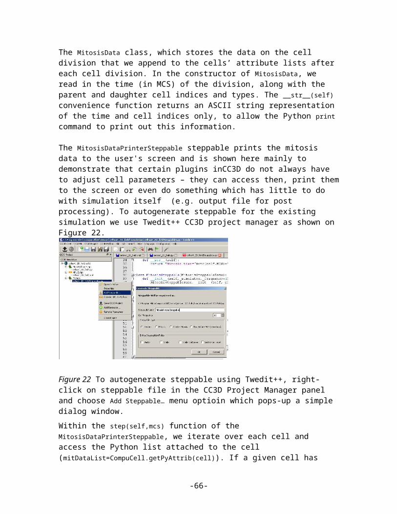
9 XML Syntax of CompuCell3D modules
9.1 Potts SectionThe first section of the .xml file defines the global parameters of the lattice and the simulation. <Potts> <Dimensions x="101" y="101" z="1"/> <Anneal>0</Anneal> <Steps>1000</Steps> <FluctuationAmplitude>5</ FluctuationAmplitude > <Flip2DimRatio>1</Flip2DimRatio> <Boundary_y>Periodic</Boundary_y> <Boundary_x>Periodic</Boundary_x> <NeighborOrder>2</NeighborOrder> <DebugOutputFrequency>20</DebugOutputFrequency> <RandomSeed>167473</RandomSeed> <EnergyFunctionCalculator Type="Statistics"> <OutputFileName Frequency="10">statData.txt</OutputFileName> <OutputCoreFileNameSpinFlips Frequency="1" GatherResults="" OutputAccepted="" OutputRejected="" OutputTotal="">
statDataSingleFlip </OutputCoreFileNameSpinFlips>
</EnergyFunctionCalculator> </Potts>
This section appears at the beginning of the configuration file. Line <Dimensions x="101" y="101" z="1"/> declares the dimensions of the lattice to be 101 x 101 x 1, i.e., the lattice is two-dimensional and extends in the xy plane. The basis of the lattice is 0 in each direction, so the 101 lattice sites in the x and y directions have indices ranging from 0 to 100. <Steps>1000</Steps> tells CompuCell how long the simulation lasts in MCS. After executing this number of steps, CompuCell can run simulation at zero temperature for an additional period. In our case it will run for <Anneal>10</Anneal> extra steps. FluctuationAmplitude parameter determines intrinsic fluctuation or motility of cell membrane. Fluctuation amplitude is a temperature parameter in classical GGH model formulation. We have decided tyo use FluctuationAmplitude term instead of temperature because using word “temperature” to describe intrinsic motility of cell membrane was quite confusing.
In the above example, fluctuation amplitude applies to all cells in the simulation. To define fluctuation amplitude separately for each cell type we use the following syntax:<FluctuationAmplitude> <FluctuationAmplitudeParameters CellType="Condensing"\ FluctuationAmplitude="10"/> <FluctuationAmplitudeParameters CellType="NonCondensing”\ FluctuationAmplitude="5"/></FluctuationAmplitude>
When CompuCell3D encounters expanded definition of FluctuationAmplitude it will use it in place of a global definition –
-66-

<FluctuationAmplitude>5</ FluctuationAmplitude >
To complete the picture CompUCell3D allows users to set fluctuation amplitude individually for each cell. Using Python scripting we write:
for cell in self.cellList: if cell.type==1: cell.fluctAmpl=20
When determining which value of fluctuation amplitude to use, CompuCell first checks if fluctAmpl is non-negative. If this is the case it will use this value as fluctuation amplitude. Otherwise it will check if users defined fluctuation amplitude for cell types using expanded XML definition and if so it will use those values as fluctuation amplitudes. Lastly it will resort to globally defined fluctuation amplitude (Temperature). Thus, it is perfectly fine to use FluctuationAmplitude XML tags and set fluctAmpl for certain cells. In such a case CompuCell3D will use fluctAmpl for cells for which users defined it and for all other cells it will use values defined in the XML.
In GGH model, the fluctuation amplitude is determined taking into account fluctuation amplitude of “source” (expanding) cell and “destination” (being overwritten) cell. Currently CompuCell3D supports 3 type functions used to calculate resultant fluctuation amplitude (those functions take as argument fluctuation amplitude of “source” and “destination” cells and return fluctuation amplitude that is used in calculation of pixel-copy acceptance). The 3 functions are Min, Max, and ArithmeticAverage and we can set them using the following option of the Potts section:
<Potts> <FluctuationAmplitudeFunctionName> Min </FluctuationAmplitudeFunctionName>…</Potts>
By default we use Min function. Notice that if you use global fluctuation amplitude definition (Temperature) it does not really matter which function you use. The differences arise when “source” and “destination” cells have different fluctuation amplitudes.The above concepts are best illustrated by the following example:
<PythonScript>Demos/FluctuationAmplitude/FluctuationAmplitude.py\</PythonScript> <Potts> <Dimensions x="100" y="100" z="1"/> <Steps>10000</Steps> <FluctuationAmplitude>5</FluctuationAmplitude> <FluctuationAmplitudeFunctionName>ArithmeticAverage\ </FluctuationAmplitudeFunctionName> <NeighborOrder>2</NeighborOrder> </Potts>
-67-

Where in the XML section we define global fluctuation amplitude and we also use ArithmeticAverage function to determine resultant fluctuation amplitude for the pixel copy.
In python script we will periodically set higher fluctuation amplitude for lattice quadrants so that when running the simulation we can see that cells belonging to different lattice quadrants have different membrane fluctuations:
class FluctuationAmplitude(SteppableBasePy): def __init__(self,_simulator,_frequency=1): SteppableBasePy.__init__(self,_simulator,_frequency)
self.quarters=[[0,0,50,50],[0,50,50,100],\ [50,50,100,100],[50,0,100,50]]
self.steppableCallCounter=0 def step(self, mcs): quarterIndex=self.steppableCallCounter % 4 quarter=self.quarters[quarterIndex]
for cell in self.cellList: if cell.xCOM>=quarter[0] and cell.yCOM>=quarter[1] and\ cell.xCOM<quarter[2] and cell.yCOM<quarter[3]:
cell.fluctAmpl=50 else:
#this means CompuCell3D will use globally defined FluctuationAmplitude cell.fluctAmpl=-1
self.steppableCallCounter+=1Assigning negative fluctuationAmplitude cell.fluctAmpl=-1 is interpreted by CompuCell3D as a hint to use fluctuation amplitude defined in the XML.
The below section describes Temperature and CellMotility tags which are beibng deprecated (however cor compatibility reasons we still support those):
The first section of the .xml file defines the global parameters of the lattice and the simulation. <Potts> <Dimensions x="101" y="101" z="1"/> <Anneal>0</Anneal> <Steps>1000</Steps> <Temperature>5</Temperature> <Flip2DimRatio>1</Flip2DimRatio> <Boundary_y>Periodic</Boundary_y> <Boundary_x>Periodic</Boundary_x> <NeighborOrder>2</NeighborOrder> <DebugOutputFrequency>20</DebugOutputFrequency>
-68-
<RandomSeed>167473</RandomSeed> <EnergyFunctionCalculator Type="Statistics"> <OutputFileName Frequency="10">statData.txt</OutputFileName> <OutputCoreFileNameSpinFlips Frequency="1" GatherResults="" OutputAccepted="" OutputRejected="" OutputTotal="">
statDataSingleFlip </OutputCoreFileNameSpinFlips>
</EnergyFunctionCalculator> </Potts>
This section appears at the beginning of the configuration file. Line <Dimensions x="101" y="101" z="1"/> declares the dimensions of the lattice to be 101 x 101 x 1, i.e., the lattice is two-dimensional and extends in the xy plane. The basis of the lattice is 0 in each direction, so the 101 lattice sites in the x and y directions have indices ranging from 0 to 100. <Steps>1000</Steps> tells CompuCell how long the simulation lasts in MCS. After executing this number of steps, CompuCell can run simulation at zero temperature for an additional period. In our case it will run for <Anneal>10</Anneal> extra steps. Setting the temperature is as easyas writing <Temperature>5</Temperature>.
We can also set temperature (or in other words cell motility) individually for each cell type. The syntax to do this is following:
<CellMotility> <MotilityParameters CellType="Condensing" Motility="10"/> <MotilityParameters CellType="NonCondensing" Motility="5"/> </CellMotility>
You may use it in the Potts section in place of <Temperature> .
Now, as you remember from the discussion about the difference between spin-flip attempts and MCS we can specify how many spin flips should be attempted in every MCS. We specify this number indirectly by specifying the Flip2DimRatio - <Flip2DimRatio>1</Flip2DimRatio>, which tells CompuCell that it should make 1 x number of lattice sites attempts per MCS – in our case one MCS is 101x101x1 spin-flip attempts. To set 2.5x101x101x1 spin flip attempts per MCS you would write <Flip2DimRatio>2.5</Flip2DimRatio>. The next line specifies the neighbor order. The higher neighbor order the longer the Euclidian distance from a given pixel. In previous versions of CompuCell3D we have been using <FlipNeighborMaxDistance> or <Depth> (in Contact energy plugins) flag to accomplish same task. Since now CompuCell3D supports two kinds of latices it would be inconvenient to change distances. It is much easier to think in terms n-th nearest neighbors. For the backwards compatibility we still support old flags but we discourage its use, especially that in the future we might support more than just two lattice types.Using nearest neighbor interactions may cause artifacts due to lattice anisotropy. The longer the interaction range, the more isotropic the simulation and the slower it runs. In addition, if the interaction range is comparable to the cell size, you may generate unexpected effects, since non-adjacent cells will contact each other.
-69-
, 07/31/09,
We can also define temperature by cell type. Can we have different temperature for each cell?
, 07/31/09,
in terms of nth nearest neighbors.

On hex lattice those problems seem to be less seveare and there 1st or 2nd nearest neighbor usually are sufficient.The Potts section also contains tags called <Boundary_y> and <Boundary_x>.These tags impose boundary conditions on the lattice. In this case the x and y axes are periodic (<Boundary_x>Periodic</Boundary_x>) so that e.g. the pixel with x=0, y=1, z=1 will neighbor the pixel with x=100, y=1, z=1. If you do not specify boundary conditions CompuCell will assume them to be of type no-flux, i.e. lattice will not be extended. The conditions are independent in each direction, so you can specify any combination of boundary conditions you like.DebugOutputFrequency is used to tell CompuCell3D how often it should output text information about the status of the simulation. This tag is optional.RandomSeed is used to initialize random number generator. If you do not do this all simulations will use same sequence of random numbers. Something you may want to avoid in the real simulations but is very useful while debugging your models.EnergyFunctionCalculator is another option of Potts object that allows users to output statistical data from the simulation for further analysis. The OutputFileName tag is used to specify the name of the file to which CompuCell3D will write average changes in energies returned by each plugins with corresponding standard deviations for those MCS whose values are divisible by the Frequency argument. Here it will write these data every 10 MCS.A second line with OutputCoreFileNameSpinFlips tag is used to tell CompuCell3D to output energy change for every plugin, every spin flip for MCS' divisible by the frequency. Option GatherResults=”” will ensure that there is only one file written for accepted (OutputAccepted), rejected (OutputRejected)and accepted and rejected (OutputTotal) spin flips. If you will not specify GatherResults CompuCell3D will output separate files for different MCS's and depending on the Frequency you may end up with many files in your directory.
One option of the Potts section that we have not used here is the ability to customize acceptance function for Metropolis algorithm:
<Offset>-0.1</Offset><KBoltzman>1.2</KBoltzman>
This ensures that spin flips attempts that increase the energy of the system are accepted with probability
where and k are specified by Offset and KBoltzman tags respectively. By default =0 and k=1.
As an alternative to exponential acceptance function you may use a simplified version which is essentially 1 order expansion of the exponential:
P=1− E−δkT
To be able to use this function all you need to do is to add the following line in the Pots section:
-70-
, 07/31/09,
is
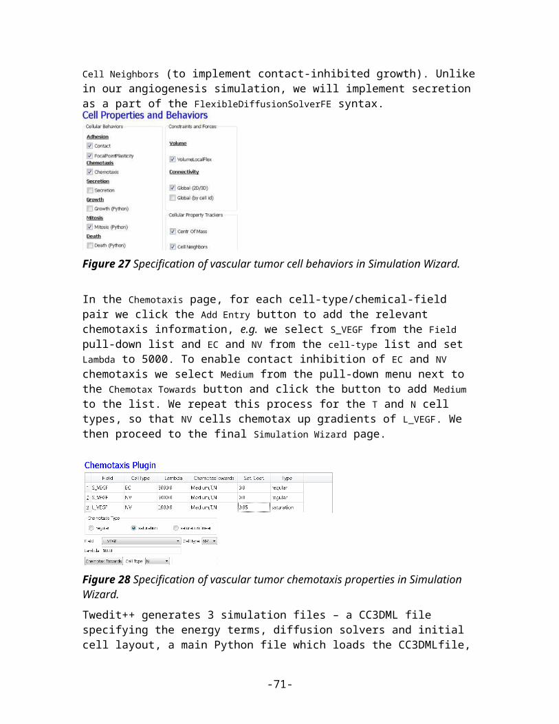
<AcceptanceFunctionName>FirstOrderExpansion</AcceptanceFunctionName>
9.1.1 Lattice Type
Early versions of CompuCell3D allowed users to use only square lattice. Most recent versions however, allow the simulation to be run on hexagonal lattice as well.To enable hexagonal lattice you need to put
<LatticeType>Hexagonal</LatticeType>
in the Potts section of the XML configuration file.
There are few things to be aware of. When using hexagonal lattice. Obviously your pixels are hexagons (2D) or rhombic dodecahedrons (3D) but what is more important is that surface or perimeter of the pixel (depending whether in 2D or 3D) is different than in the case of sqaure pixel. The way CompuCell3D hex lattice implementation was done was that the volume of the pixel was constrained to be 1 regardless of the lattice type.Second, there is one to one correspondence between pixels of the square lattice and pixels of the hex lattice. Consequently we can come up with transformation equations which give positions of hex pixels as a function of square lattice pixel position:
Based on the above facts one can work out how unit length and unit surface transform to the hex lattice. The conversion factors are given below:For the 2D case, assuming that each pixel has unit volume, we get:
-71-
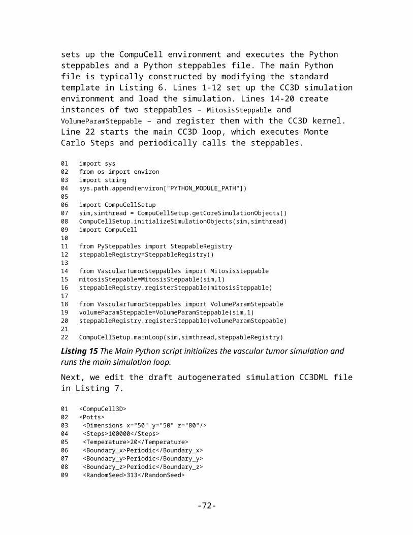
where Shex−unit denotes length of the hexagon and Lhex−unit denotes a distance between centers of the hexagons. Notice that unit surface in 2D is simply a length of the hexagon side and surface area of the hexagon with side 'a' is:
In 3D we can derive the corresponding unit quantities starting with the formulae for Volume and surface of rhombic dodecahedron (12 hedra)
where 'a' denotes length of dodecahedron edge.Constraining the volume to be one we get
and thus unit surface is given by:
and unit length by:
9.2 Plugins Section
In this section we overview XML syntax for all the plugins available in CompuCell3D. Plugins are either energy functions, lattice monitors or store user assigned data that CompuCell3D uses internally to configure simulation before it is run.
9.2.1 CellType PluginAn example of the plugin that stores user assigned data that is used to configure simulation before it is run is a CellType Plugin. This plugin is responsible for defining cell types and storing cell type information. It is a basic plugin used by virtually every CompuCell simulation. The syntax is straight forward as can be seen in the example below:
<Plugin Name="CellType"> <CellType TypeName="Medium" TypeId="0"/> <CellType TypeName="Fluid" TypeId="1"/> <CellType TypeName="Wall" TypeId="2" Freeze=""/>
-72-
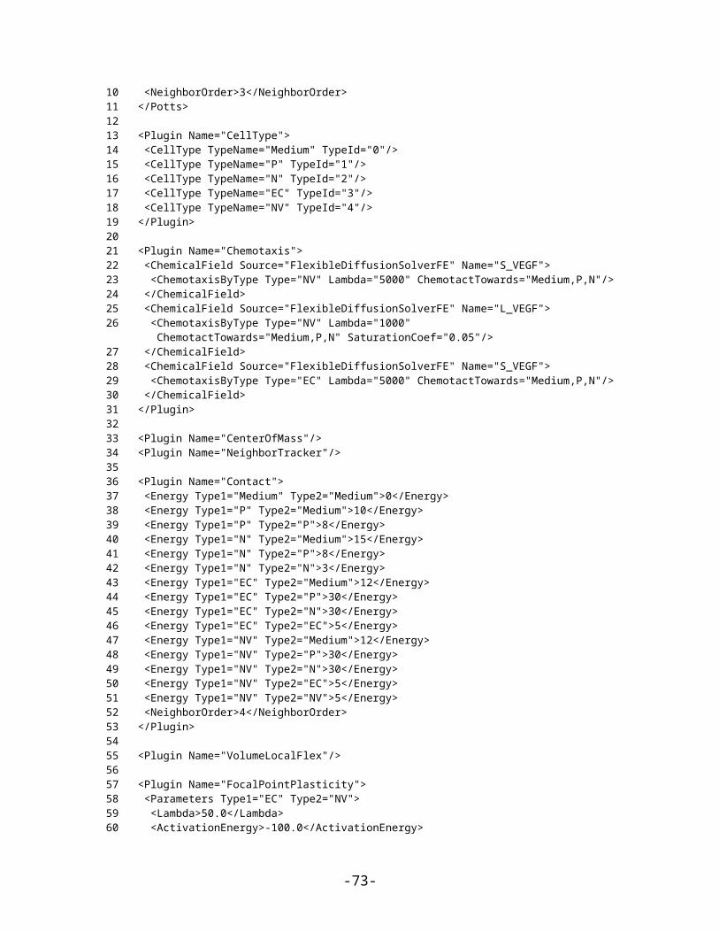
</Plugin>
Here we have defined three cell types that will be present in the simulation: Medium,Fluid,Wall. Notice that we assign a number – TypeId – to every cell type. It is strongly recommended that TypeId’s are consecutive positive integers (e.g. 0,1,2,3...). Medium is traditionally given TypeId=0 but this is not a requirement. However every CC3D simulation mut define CellType Plugin and include at least Medium specification.
Notice that in the example above cell type “Wall” has extra attribute Freeze=””. This attribute tells CompuCell that cells of “frozen” type will not be altered by spin flips. Freezing certain cell types is a very useful technique in constructing different geometries for simulations or for restricting ways in which cells can move. In the example below we have frozen cell types wall to create tube geometry for fluid flow studies.
9.2.2 Simple Volume and Surface Constraints
One of the most commonly used energy term in the GGH Hamiltonian is a term that restricts variation of single cell volume. Its simplest form can be coded as show below:
<Plugin Name="Volume"> <TargetVolume>25</TargetVolume> <LambdaVolume>2.0</LambdaVolume> </Plugin>
By analogy we may define a term which will put similar constraint regarding the surface of the cell:
<Plugin Name="Surface"> <TargetSurface>20</TargetSurface> <LambdaSurface>1.5</LambdaSurface> </Plugin>
These two plugins inform CompuCell that the Hamiltonian will have two additional terms associated with volume and surface conservation. That is when spin flip is attempted one cell will increase its volume and another cell will decrease. Thus overall energy of the system may or will change. Volume constraint essentially ensures that cells maintain the volume which close (this depends on thermal fluctuations) to target volume . The role of surface plugin is analogous to volume, that is to “preserve” surface. Note that surface plugin is commented out in the example above.
Energy terms for volume and surface constraints have the form:
Remark:
-73-

Notice that flipping a single spin may cause surface change in more that two cells – this is especially true in 3D.
9.2.3 VolumeTracker and SurfaceTracker plugins
These two plugins monitor lattice and update volume and surface of the cells once spin flip occurs. In most cases users will not call those plugins directly. They will be called automatically when either Volume (calls Volume Tracker) or Surface (calls Surface Tracker) or CenterOfMass (calls VolumeTracker) plugins are requested. However one should be aware that in some situations, for example when doing foam coarsening simulation as presented in the introduction, when neither Volume or Surface plugins are called, one may still want to track changes ion surface or volume of cells . In such situations one can explicitely invoke VolumeTracker or Surface Tracker plugin with the following syntax:
<Plugin Name=”VolumeTracker”/>
<Plugin Name=”SurfaceTracker”/>
9.2.4 VolumeFlex Plugin
VolumeFlex plugin is more sophisticated version of Volume Plugin. While Volume Plugin treats all cell types the same i.e. they all have the same target volume and lambda coefficient, VolumeFlex plugin allows you to assign different lambda and different target volume to different cell types. The syntax for this plugin is straightforward and essentially mimics the example below.
<Plugin Name="VolumeFlex"> <VolumeEnergyParameters CellType="Prestalk" TargetVolume="68" LambdaVolume="15"/> <VolumeEnergyParameters CellType="Prespore" TargetVolume="69" LambdaVolume="12"/> <VolumeEnergyParameters CellType="Autocycling" TargetVolume="80" LambdaVolume="10"/> <VolumeEnergyParameters CellType="Ground" TargetVolume="0" LambdaVolume="0"/> <VolumeEnergyParameters CellType="Wall" TargetVolume="0" LambdaVolume="0"/></Plugin>
Notice that in the example above cell types Wall and Ground have target volume and coefficient lambda set to 0 – very unusual. That's because in this particular those cells are were frozen so the parameters specified for these cells do not matter. In fact it is safe to remove specifications for these cell types, but just for the illustration purposes we left them.
Using VolumeFlex Plugin you can effectively freeze certain cell types. All you need to do is to put very high lambda coefficient for the cell type you wish to freeze. You have to be careful though , because if initial volume of the cell of a given type is different from target volume for this cell type the cells will either shrink or expand to match target volume (this is out of control and you should avoid it), and only after this initial volume adjustment will they remain frozen . That is provided LambdaVolume is high enough. In
-74-

any case, we do not recommend this way of freezing cells because it is difficult to use, and also not efficient in terms of speed of simulation run.
9.2.5 SurfaceFlex Plugin
SurfaceFlex plugin is more sophisticated version of Surface Plugin. Everything that was said with respect to VolumeFlex plugin applies to SurfaceFlex. For syntax see example below:
<Plugin Name="SurfaceFlex"> <SurfaceEnergyParameters CellType="Prestalk" TargetSurface="90" LambdaSurface="0.15"/> <SurfaceEnergyParameters CellType="Prespore" TargetSurface="98" LambdaSurface="0.15"/> <SurfaceEnergyParameters CellType="Autocycling" TargetSurface="92" LambdaSurface="0.1"/> <SurfaceEnergyParameters CellType="Ground" TargetSurface="0" LambdaSurface="0"/> <SurfaceEnergyParameters CellType="Wall" TargetSurface="0" LambdaSurface="0"/> </Plugin>
9.2.6 VolumeLocalFlex Plugin
VolumeLocalFlex Plugin is very similar to Volume plugin. You specify both lambda coefficient and target volume, but as opposed to Volume Plugin the energy is calculated using target volume and lambda volume that are specified individually for each cell. In the course of simulation you can change this target volume depending on e.g. concentration of FGF in the particular cell. This way you can specify which cells grow faster, which slower based on a state of the simulation. This plugin requires you to develop a module (plugin or steppable) which will alter target volume for each cell. You can do it either in C++ or even better in Python.
Example syntax:
<Plugin Name="VolumeLocalFlex"/>
9.2.7 SurfaceLocalFlex Plugin
This plugin is analogous to VolumeLocalFlex but operates on cell surface.
Example syntax:
<Plugin Name="SurfaceLocalFlex"/>
9.2.8 NeighborTracker Plugin
This plugin, as its name suggests, tracks neighbors of every cell. In addition it calculates common contact area between cell and its neighbors. We consider a neighbor this cell that has at least one common pixel side with a given cell. This means that cells that touch
-75-

each other either “by edge” or by “corner” are not considered neighbors. See the drawing below:
5 5 5 4 4
5 5 5 4 4
5 5 4 4 4
1 1 2 2 2
1 1 2 2 2
Figure 19. Cells 5,4,1 are considered neighbors as they have non-zero common surface area. Same applies to pair of cells 4 ,2 and to 1 and 2. However, cells 2 and 5 are not neighbors because they touch each other “by corner”. Notice that cell 5 has 8 pixels cell 4 , 7 pixels, cell 1 4 pixels and cell 2 6 pixels.
Example syntax:
<Plugin Name="NeighborTracker"/>
This plugin is used as a helper module by other plugins and steppables e.g. Elasticity and AdvectionDiffusionSolver use NeighborTracker plugin.
9.2.9 Chemotaxis
Chemotaxis plugin , as its name suggests is used to simulate chemotaxis of cells. For every spin flip this plugin calculates change of energy associated with pixel move. There are several methods to define a change in energy due to chemotaxis. By default we define a chemotaxis using the following formula:
where
, denote chemical concentration at the spin-flip-source and spin-flip-destination pixel. respectively.
We also support a slight modification of the above formula in the Chemotaxis plugin where is non-zero only if the cell located at after the spin flip is non-medium. to enable such mode users need to include <Algorithm=”Regular”/> tag in the body of XML plugin.
Let's look at the syntax by studying the example usage of the Chemotaxis plugin:
-76-
, 07/31/09,
Destination means”source”
, 07/31/09,
Not sure about the sign

<Plugin Name="Chemotaxis"> <ChemicalField Source="FlexibleDiffusionSolverFE" Name="FGF"> <ChemotaxisByType Type="Amoeba" Lambda="300"/> <ChemotaxisByType Type="Bacteria" Lambda="200"/> </ChemicalField> </Plugin>
The body of the chemotaxis plugin description contains sections called ChemicalField. In this section you tell CompuCell3D which module contains chemical field that you wish to use for chemotaxis. In our case it is FlexibleDiffusionSolverFE. Next you need to specify the name of the field - FGF in our case. Next you specify lambda for each cell type so that cells of different type may respond differently to a given chemical. In particular types not listed will not respond to chemotaxis at all. Older versions of CompuCell3D allowed for different syntaxes as well. Despite the fact that those syntaxes are still supported for backward compatibility reasons, we discourage their use, because, they are somewhat confusing.
Ocassionally you may want to use different formula for the chemotaxis than the one presented above. Current CompCell3D allows you to use the following definitions of change in chemotaxis energy (Saturation and SaturationLinear respectively ):
or
where 's' denotes saturation constant. To use first of the above formulas all you need to do is to let CompuCell3D know the value of the saturation coefficient:
<Plugin Name="Chemotaxis"> <ChemicalField Source="FlexibleDiffusionSolverFE" Name="FGF"> <ChemotaxisByType Type="Amoeba" Lambda="0"/> <ChemotaxisByType Type="Bacteria" Lambda="2000000" SaturationCoef="1"/> </ChemicalField> </Plugin>
Notice that this only requires small change in line where you previously specified only lambda.
<ChemotaxisByType Type="Bacteria" Lambda="2000000" SaturationCoef="1"/>
-77-
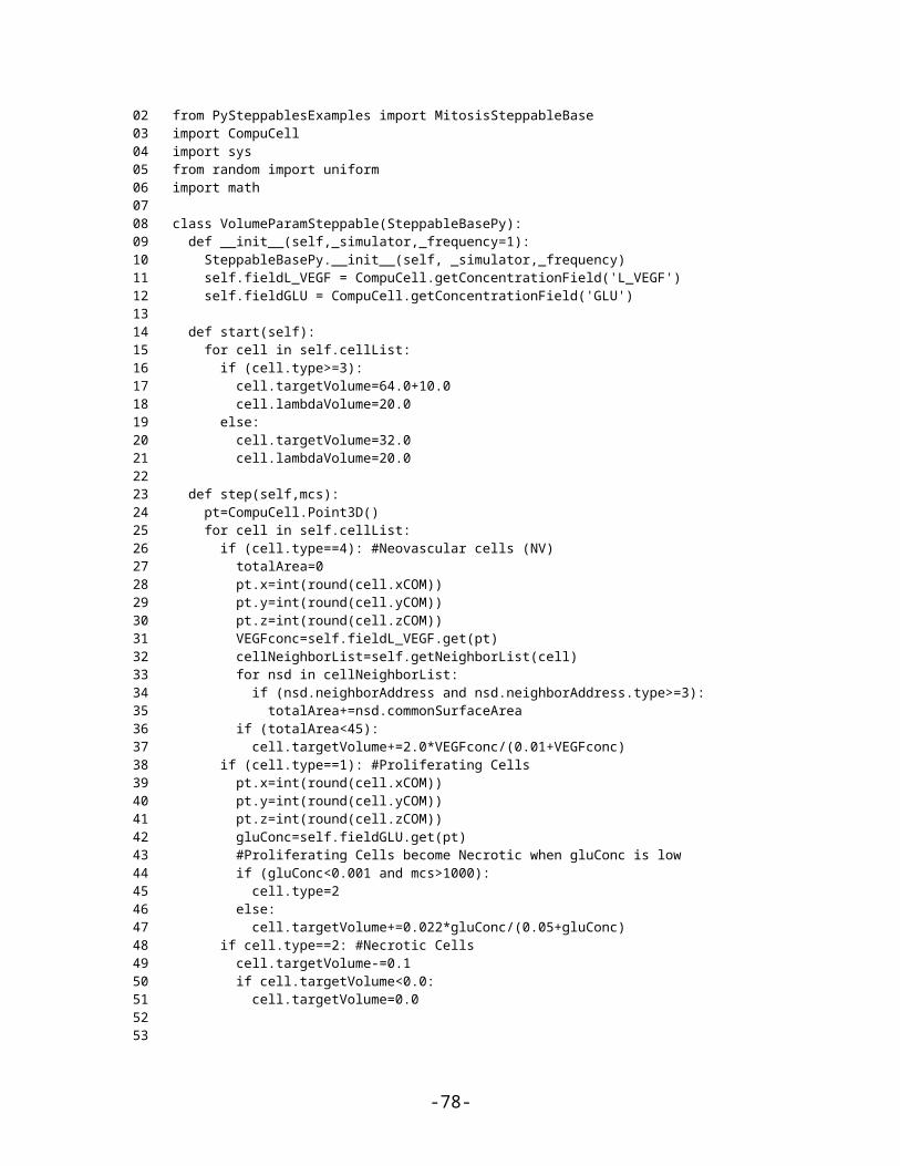
To use second of the above formulas use SaturationLinearCoef instead of SaturationCoef:
<Plugin Name="Chemotaxis"> <ChemicalField Source="FlexibleDiffusionSolverFE" Name="FGF"> <ChemotaxisByType Type="Amoeba" Lambda="0"/> <ChemotaxisByType Type="Bacteria" Lambda="2000000" SaturationLinearCoef="1"/> </ChemicalField> </Plugin>
Sometimes it is desirable to have chemotaxis between only certain types of cells and not between other pairs of types. To deal with this situation it is enough to augment ChemotaxisByType element with the following attribute:
<ChemotaxisByType Type="Amoeba" Lambda="100 "ChemotactTowards="Medium" />
This will cause that the change in chemotaxis energy will be non-zero only for those spin flip attempts that will try to slip Amoeba and Medium pixels.
The definitions of chemotaxis presented so far do not allow specification of chemotaxis parameters individually for each cell. To do this we will use Python scripting. We still need to specify in the XML which fields are important from chamotaxis stand point. Only fields listed in the XML will be used to calculate chemotaxis energy:…<Plugin Name="CellType"> <CellType TypeName="Medium" TypeId="0"/> <CellType TypeName="Bacterium" TypeId="1" /> <CellType TypeName="Macrophage" TypeId="2"/> <CellType TypeName="Wall" TypeId="3" Freeze=""/> </Plugin>…<Plugin Name="Chemotaxis"> <ChemicalField Source="FlexibleDiffusionSolverFE" Name="ATTR"> <ChemotaxisByType Type="Macrophage" Lambda="20"/> </ChemicalField> </Plugin>…In the above excerpt from the XML configuration file we see that cells of type Macrophage will chemotax in response to ATTR gradient.
Using Python scripting we can modify chemotaxing properties of individual cells as follows:class ChemotaxisSteering(SteppableBasePy): def __init__(self,_simulator,_frequency=100): SteppableBasePy.__init__(self,_simulator,_frequency) def start(self):
-78-
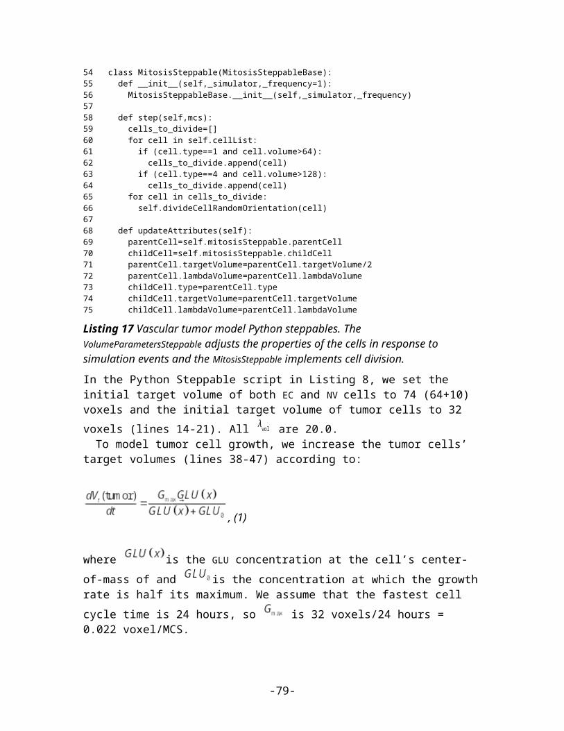
for cell in self.cellList: if cell.type==2: cd=self.chemotaxisPlugin.addChemotaxisData(cell,"ATTR") cd.setLambda(20.0)
# cd.initializeChemotactTowardsVectorTypes("Bacterium,Medium") cd.assignChemotactTowardsVectorTypes([0,1])
break def step(self,mcs): for cell in self.cellList: if cell.type==2: cd=self.chemotaxisPlugin.getChemotaxisData(cell,"ATTR") if cd: l=cd.getLambda()-3 cd.setLambda(l) break
In the start function for first encountered cell of type Macrophage (type==2) we insert ChemotaxisData object (it determines chemotaxing properties) and initialize parameter to 20. We also initialize vector of cell types towards which Macrophage cell will chemotax (it will chemotax towards Medium and Bacterium cells). Notice the break statement inside the if statement, inside the loop. It ensures that only first encountered Macrophage cell will have chemotaxing properties altered. In the step function we decrease lambda chemotaxis by 3 units every 100 MCS. In effect we turn a cell from chemotaxing up ATTR gradient to being chemorepelled.
In the above example we have more than one macrophage but only one of them has altered chemotaxing properties. The other macrophages have chemotaxing properties set itn eh XML section. CompuCell3D first checks if local definitions of chemotaxis are available (i.e. for individual cells) and if so it uses those. Otherwise it will use definitions from from the XML.
The ChemotaxisData structure has additional functions which allo to set chemotaxis formula used. For example we may type: def start(self): for cell in self.cellList: if cell.type==2: cd=self.chemotaxisPlugin.addChemotaxisData(cell,"ATTR") cd.setLambda(20.0) cd.setSaturationCoef(200.0)
# cd.initializeChemotactTowardsVectorTypes("Bacterium,Medium") cd.assignChemotactTowardsVectorTypes([0,1])
break
-79-

to activate Saturation formula. To activate SaturationLinear formula we would use:
cd.setSaturationLinearCoef(2.0)
CAUTION: when you use chemotaxis plugin you have to make sure that fields that you refer to and module that contains this fields are declared in the xml file. Otherwise you will most likely cause either program crash (which is not as bad as it sounds) or unpredicted behavior (much worse scenario, although unlikely as we made sure that in the case of undefined symbols, CompuCell3D exits)
9.2.10 ExternalPotential plugin
Chemotaxis plugin is used to cause directional cell movement. Another way to achieve directional movement is to use ExternalPotential plugin. This plugin is responsible for imposing a directed pressure (or rather force) on cells. It is used mainly in fluid flow studies with periodic boundary conditions along these coordinates along which force acts. If NoFlux boundary conditions are set instead , the cells will be squeezed.
This is the example usage of this plugin:
<Plugin Name="ExternalPotential"> <Lambda x="-0.5" y="0.0" z="0.0"/> </Plugin>
Lambda is a vector quantity and determines components of force along three axes. In this case we apply force along x. We can also apply external potential to specific cell types:
<Plugin Name="ExternalPotential"> <ExternalPotentialParameters CellType="Body1" x="-10" y="0" z="0"/> <ExternalPotentialParameters CellType="Body2" x="0" y="0" z="0"/> <ExternalPotentialParameters CellType="Body3" x="0" y="0" z="0"/></Plugin>
Where in ExternalPotentialParameters we specity which cell type is subject to external potential (Lambda is specified using x,y,z attributes).
We can also apply external potential to individual cells. In that case, in the XML section we only need to specify:
<Plugin Name="ExternalPotential"/>
and in the Python file we change lambdaVecX, lambdaVecY, lambdaVecZ, which are properties of cell. For example in Python we could write:
cell.lambdaVecX=-10
-80-
Calculations done by ExternalPotential Plugin are by default based on direction of pixel copy (similarly as in chemotaxis plugin). One can however force CC3D to do calculations based on movement of center of mass of cell. To use algorithm based on center of mass movement we use the following XML syntax:
<Plugin Name="ExternalPotential"> <Algorithm>CenterOfMassBased</Algorithm>…</Plugin>Remark:Note that in the pixel-based algorithm the typical value of pixel displacement used in calculations is of the order of 1 (pixel) whereas typical displacement of center of mass of cell due to single pixel copy is of the order of 1/cell volume (pixels) – ~ 0.1 pixel. This implies that to achieve compatible behavior of cells when using center of mass algorithm we need to multiply lambda’s by appropriate factor, typicall of the order of 10.
9.2.11 CellOrientation Plugin
Similarly as ExternalPotential plugin this plugin gives preference to those pixel copies whose direction aligns with polarization vector (which is a property of each cell):ΔE=− λ(σ ( i))∗ p (σ ( i))⋅c ,where (i) denotes cell at site i, p is polarization vector for cell at site i and c pixel copy vector. Because two cell participate in the pixel copy process the net energy change is simply a sum of above expressions: one for growing cell and one for shrinking cell. To set lambda we have two options: use global setting in the XML:
<Plugin Name="CellOrientation"> <LambdaCellOrientation>0.5</LambdaCellOrientation> </Plugin>
Or set individually for each cell and manage values of from Python. In this case we use the following XML syntax:
<Plugin Name="CellOrientation"> <LambdaFlex/> </Plugin>
or equivalently the shorter version:
<Plugin Name="CellOrientation"/>
If we manage values in Python we would use the following syntax to acces and modify values of lambda:
self.cellOrientationPlugin.getLambdaCellOrientation(cell)
self.cellOrientationPlugin.setLambdaCellOrientation(cell,0.5)
-81-

Calculations done by CellOrientation Plugin are by default based on direction of pixel copy (similarly as in chemotaxis plugin). One can however force CC3D to do calculations based on movement of center of mass of cell. To use algorithm based on center of mass movement we use the following XML syntax:
<Plugin Name="CellOrientation"> <Algorithm>CenterOfMassBased</Algorithm>…</Plugin>See remark in External potential description about rescaling of parameters when changing algorithm to Center Of Mass–based.
9.2.12 PolarizationVector Plugin
PolarizationVector plugin is a simple plugin whose only task is to ensure that each cell in CompuCell3D simulation has as its attribute 3-component vector of floating point numbers. This plugin is normally used in together with CellOrientation but it also can be reused in other applications, assuming that we do not use CellOrientation plugin at the same time. The XML syntax is very simple:
<Plugin Name="PolarizationVector"/>
To access or modify polarization vector requires use of Python scripting.
self.polarizationPlugin.getPolarizationVector(cell)
or to change values of the polarization vector:
self.polarizationPlugin.getPolarizationVector(cell,0.1,0.2,0.3)
9.2.13 CenterOfMass Plugin
This plugin monitors changes n the lattice and updates centroids of the cell:xCM=∑
ix i , yCM=∑
iy i , zCM=∑
iz i
where i denotes pixels belonging to a given cell. To obtain coordinates of a center of mass f a given cell you need to divide centroids by cell volume:
XCM =xCM
V, Y CM =
yCM
V, ZCM=
zCM
V
This plugin is aware of boundary conditions and centroids are calculated properly regardless which boundary conditions are used. The XML syntax is very simple:
<Plugin Name="CenterOfMass"/>
-82-
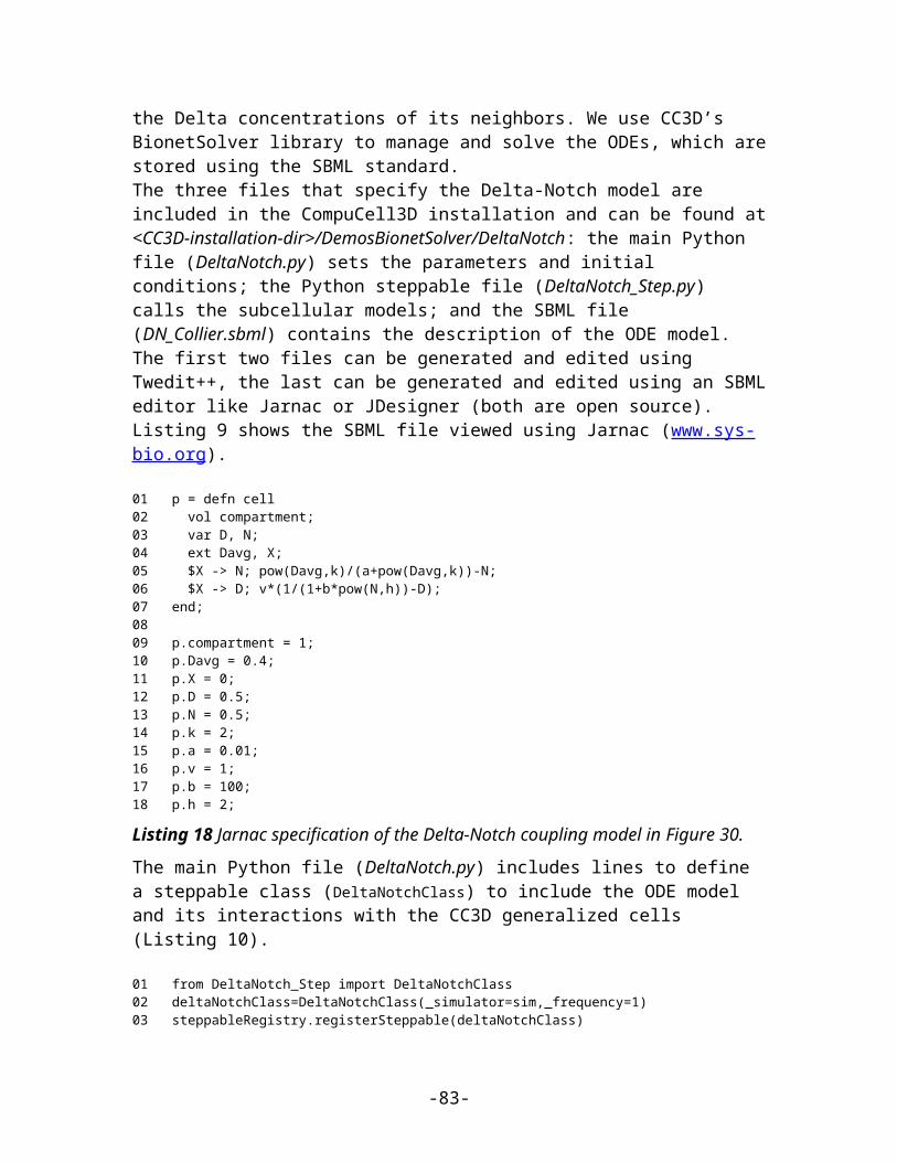
9.2.14 Contact Energy
Energy calculations for the foam simulation are based on the boundary or contact energy between cells (or surface tension, if you prefer). Together with volume constraint contact energy is one of the most commonly used energy terms in the GGH Hamiltonian. In essence it describes how cells "stick" to each other.
The explicit formula for the energy is:
,
where i and j label two neighboring lattice sites , 's denote cell Ids, 's denote cell types . In the case of foam simulation the total energy of the foam is simply the total boundary length times the surface tension (here defined to be 2J).
Once again, in the above formula, you need to differentiate between cell types and cell Ids. This formula shows that cell types and cell Ids are not the same. The Contact plugin in the .xml file, defines the energy per unit area of contact between cells of different types
( ) and the interaction range (NeighborOrder) of the contact:
<Plugin Name="Contact"> <Energy Type1="Foam" Type2="Foam">3</Energy> <Energy Type1="Medium" Type2="Medium">0</Energy> <Energy Type1="Medium" Type2="Foam">0</Energy> <NeighborOrder>2</NeighborOrder> </Plugin>
In this case, the interaction range is 2, thus only up to second nearest neighbor pixels of a pixel undergoing a change or closer will be used to calculate contact energy change. Foam cells have contact energy per unit area of 3 and Foam and Medium as well as Medium and Medium have contact energy of 0 per unit area.
9.2.15 ContactLocalProduct Plugin
This plugin calculates contact energy based on local (i.e. per cell) cadhering expression levels. This plugin has to be used in conjunction with a steppable that assigns cadherin expression levels to the cell. Such steppables are usually written in Python – see ContactLocalProductExample in Demos directory.
We use the following formulas to calculate energy for this plugin:
-83-
, 07/31/09,
Do we show an example?

By default . is a function of cadherins and can be either a simple
product , a product of squared expression levels or a
.
In the case of the second formula plays the role of “regular” contact energy between cell and medium.
The syntax of this plugin is as follows:
<Plugin Name="ContactLocalProduct"> <ContactSpecificity Type1="Medium" Type2="Medium">0</ContactSpecificity> <ContactSpecificity Type1="Medium" Type2="CadExpLevel1">-16</ContactSpecificity> <ContactSpecificity Type1="Medium" Type2="CadExpLevel2">-16</ContactSpecificity> <ContactSpecificity Type1="CadExpLevel1" Type2="CadExpLevel1">-2</ContactSpecificity> <ContactSpecificity Type1="CadExpLevel1" Type2="CadExpLevel2">2.75</ContactSpecificity> <ContactSpecificity Type1="CadExpLevel2" Type2="CadExpLevel2">-1</ContactSpecificity> <ContactFunctionType>Quadratic</ContactFunctionType> <EnergyOffset>0.0</EnergyOffset> <NeighborOrder>2</NeighborOrder> </Plugin>
Users need to specify ContactSpecificity ( ) between different cell types
ContactFunctionType (by default it is set to Linear - but other allowed key
words are Quadratic - and Min - ). EnergyOffset can be set to user specified value using above syntax. NeighborOrder has the same meaning as for “regular” Contact plugin.
Alternatively one can write customized function of the two cadherins and use it instead of the 3 choices given above. To do this, simply use the following syntax: <Plugin Name="ContactLocalProduct"> <ContactSpecificity Type1="Medium" Type2="Medium">0</ContactSpecificity> <ContactSpecificity Type1="Medium" Type2="CadExpLevel1">-16</ContactSpecificity> <ContactSpecificity Type1="Medium" Type2="CadExpLevel2">-16</ContactSpecificity> <ContactSpecificity Type1="CadExpLevel1" Type2="CadExpLevel1">-2</ContactSpecificity> <ContactSpecificity Type1="CadExpLevel1" Type2="CadExpLevel2">2.75</ContactSpecificity> <ContactSpecificity Type1="CadExpLevel2" Type2="CadExpLevel2">-1</ContactSpecificity> <ContactFunctionType>Quadratic</ContactFunctionType> <EnergyOffset>0.0</EnergyOffset> <NeighborOrder>2</NeighborOrder> <CustomFunction> <Variable>J1</Variable> <Variable>J2</Variable> <Expression>sin(J1*J2)</Expression> </CustomFunction> </Plugin>
-84-
, 07/31/09,
What does it mean? Negative or positive values?
, 07/31/09,
Is it a cell type?
, 07/31/09,
It would be very helpful , if you could explain what cadExpLevel1 does in a paragraph. Does it stick to cadExpLevel2? How strong is it in comparison to cadExpLevel1 and medium?
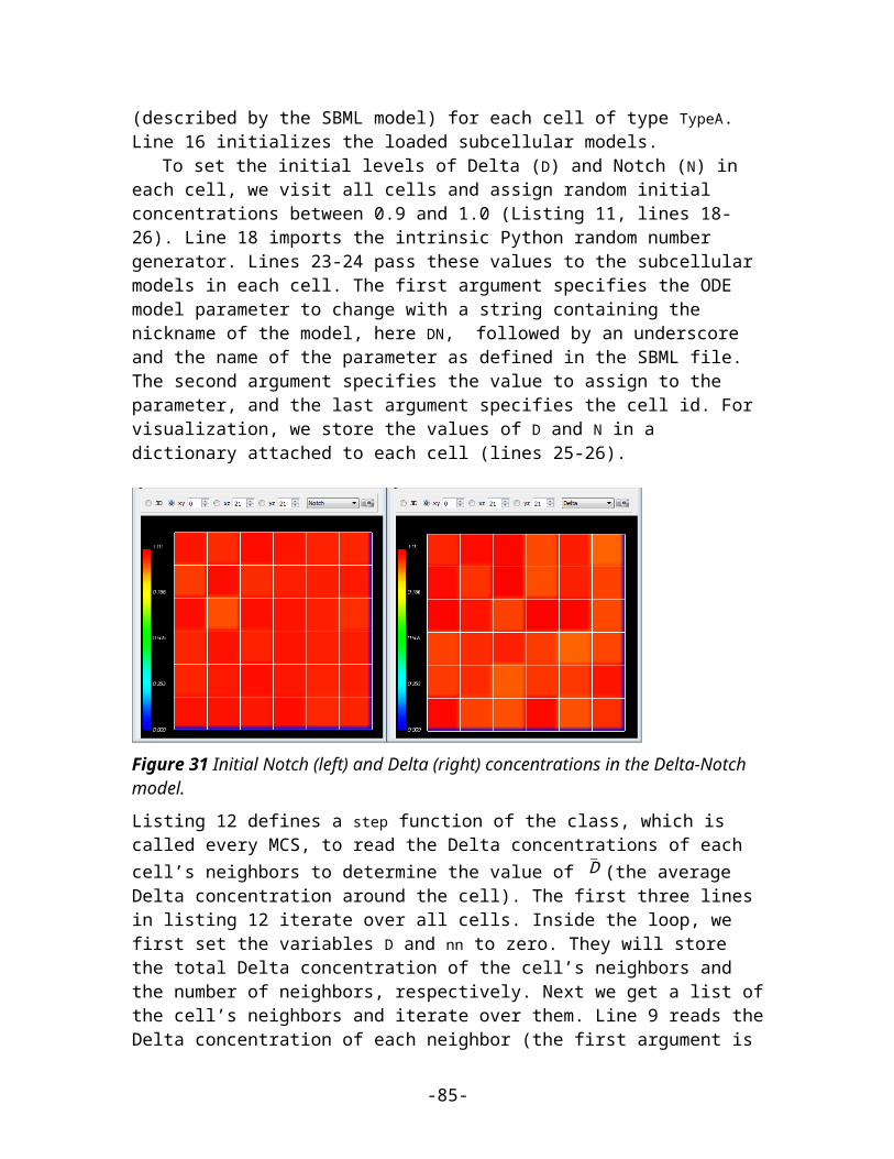
Here we define variable names for cadherins in interacting cells (J1 denotes cadherin for one of the cells and cell2 denotes cadherin for another cell). Then in the Expression tag we give mathematical expression involving the two cadherin levels. The expression syntax has to follow syntax of the muParser - http://muparser.sourceforge.net/mup_features.html#idDef2.
9.2.16 AdhesionFlex PluginAdhesion Flex is a generalization of ContactLocalProduct plugin. It allows setting individual adhesivity properties for each cell. Users can use either XML syntax or Python scripting to initialize adhesion molecule density for each cell. In addition, Medium can also carry its own adhesion molecules. We use the following formula to calculate Contact energy in AdhesionFlex plugin:
E= ∑i , j−neighbors (−∑
m,nk mn F ( Nm( i) ,N n( j )))(1−δ σ (i) , σ ( j))
where indexes i, j label pixels, denotes contact energy between cell types
and , exactly as in “regular” contact plugin and indexes m,n label cadherins in cells composed f pixels i and j respectively. F denotes user-defined function of Nm and Nn. Altohugh this may look a bit complex, the basic idea is simple: each cell has certain number of cadherins on its surface. When cell touch each other the resultant energy is
simpy a “product” -k mn F ( Nm( i) ,N n( j ))- of every cadherin from one cell with every cadherin from another cell.The XML syntax for this plugin is given below:
<Plugin Name="AdhesionFlex"> <AdhesionMolecule Molecule="NCad"/> <AdhesionMolecule Molecule="NCam"/> <AdhesionMolecule Molecule="Int"/> <AdhesionMoleculeDensity CellType="Cell1" Molecule="NCad" Density="6.1"/> <AdhesionMoleculeDensity CellType="Cell1" Molecule="NCam" Density="4.1"/> <AdhesionMoleculeDensity CellType="Cell1" Molecule="Int" Density="8.1"/> <AdhesionMoleculeDensity CellType="Medium" Molecule="Int" Density="3.1"/> <AdhesionMoleculeDensity CellType="Cell2" Molecule="NCad" Density="2.1"/> <AdhesionMoleculeDensity CellType="Cell2" Molecule="NCam" Density="3.1"/> <BindingFormula Name="Binary"> <Formula> min(Molecule1,Molecule2)</Formula> <Variables> <AdhesionInteractionMatrix> <BindingParameter Molecule1="NCad" Molecule2="NCad" > -1.0</BindingParameter> <BindingParameter Molecule1="NCam" Molecule2="NCam"> 2.0</BindingParameter>
-85-
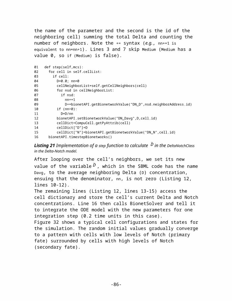
<BindingParameter Molecule1="NCad" Molecule2="NCam" > -10.0</BindingParameter> <BindingParameter Molecule1="Int" Molecule2="Int" > -10.0</BindingParameter> </AdhesionInteractionMatrix> </Variables> </BindingFormula> <NeighborOrder>2</NeighborOrder></Plugin>
kmn matrix is specified within the AdhesionInteractionMatrix tag – the elements are listed using BindingParameter tags. The AdhesionMoleculeDensity tag specifies initial concentration of adhesion molecules. Even if you are going to modify those from Python (in the start function of the steppable) you are still required to specify the names of adhesion molecules and associate them with appropriate cell types. Failure to do so may result in simulation crash or undefined behaviors. The user-defined function F is specified using Formula tag where the arguments of the function are called Molecule1 and Molecule2. The syntax has to follow syntax of the muParser - http://muparser.sourceforge.net/mup_features.html#idDef2 .
CompuCell3D example – Demos/AdhesionFlex - demonstrates how to manipulate concentration of adhesion molecules:
self.adhesionFlexPlugin.getAdhesionMoleculeDensity(cell,"NCad")
allows to access adhesion molecule concentration using its name (as given in the XML above using AdhesionMoleculeDensity tag).
self.adhesionFlexPlugin.getAdhesionMoleculeDensityByIndex(cell,1)
allows to access adhesion molecule concentration using its index in the adhesion molecule density vector. The order of the adhesion molecule densities in the vector is the same as the order in which they were declared in the XML above - AdhesionMoleculeDensity tags.
self.adhesionFlexPlugin.getAdhesionMoleculeDensityVector(cell)
allows access to entire adhesion molecule density vector.
Each of these functions has its corresponding function whith operates on Medium. In this case we do not give cell as first argument:
self.adhesionFlexPlugin.getMediumAdhesionMoleculeDensity(“Int”)
self.adhesionFlexPlugin.getMediumAdhesionMoleculeDensityByIndex (0)
-86-
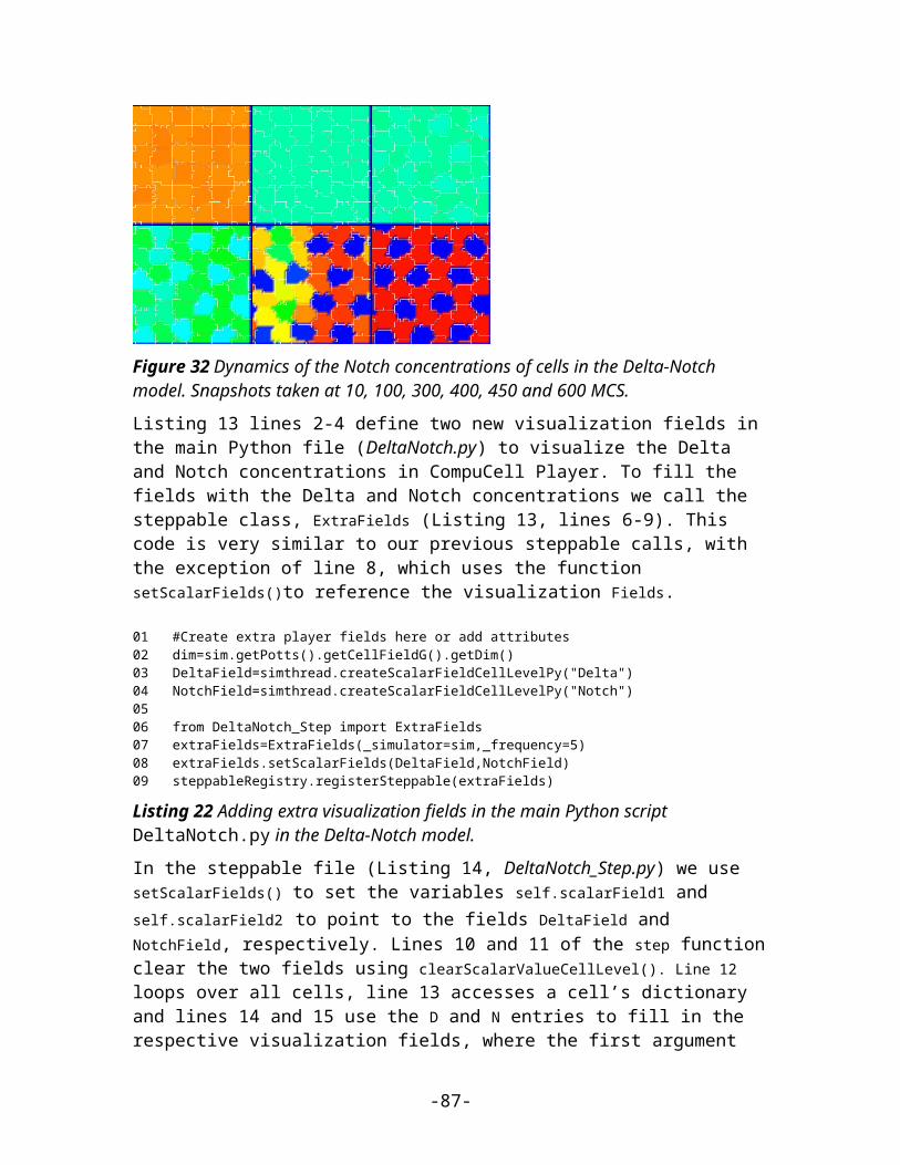
self.adhesionFlexPlugin.getMediumAdhesionMoleculeDensityVector(cell)
To change the value of the adhesion molecule density we use set functions:
self.adhesionFlexPlugin.setAdhesionMoleculeDensity(cell,"NCad",0.1)
self.adhesionFlexPlugin.setAdhesionMoleculeDensityByIndex(cell,1,1.02)
self.adhesionFlexPlugin.setAdhesionMoleculeDensityVector(cell,\[3.4,2.1,12.1])
Notice that in this las function we passed entire Python list as the argument. CC3D will check if the number of entries in this vector is the same as the number of entries in the currently used vector. If so the values from the passed vector will be copied, otherwise they will be ignored.
IMPORTANT: during mitosis we create new cell (childCell) and the adhesion molecule vector of this cell will have no components. However in order for simulation to continue we have to initialize this vector with number of cadherins appropriate to childCell type. We know that setAdhesionMoleculeDensityVector is not appropriate for this task so we have to use:
self.adhesionFlexPlugin.assignNewAdhesionMoleculeDensityVector(cell,\[3.4,2.1,12.1])
which will ensure that the content of passed vector is copied entirely into cell’s vector (making size adjustments as necessry).
IMPORTANT: You have to make sure that the number of newly assigned adhesion molecules is exactly the same as the number of adhesion molecules declared for the cell of this particular type.
All of get functions has corresponding set function which operates on Medium:
self.adhesionFlexPlugin.setMediumAdhesionMoleculeDensity("NCam",2.8)
self.adhesionFlexPlugin.setMediumAdhesionMoleculeDensityByIndex(2,16.8)
self.adhesionFlexPlugin.setMediumAdhesionMoleculeDensityVector(\[1.4,3.1,18.1])
self.adhesionFlexPlugin.assignNewMediumAdhesionMoleculeDensityVector(\[1.4,3.1,18.1])
9.2.17 ContactMultiCad Plugin
-87-
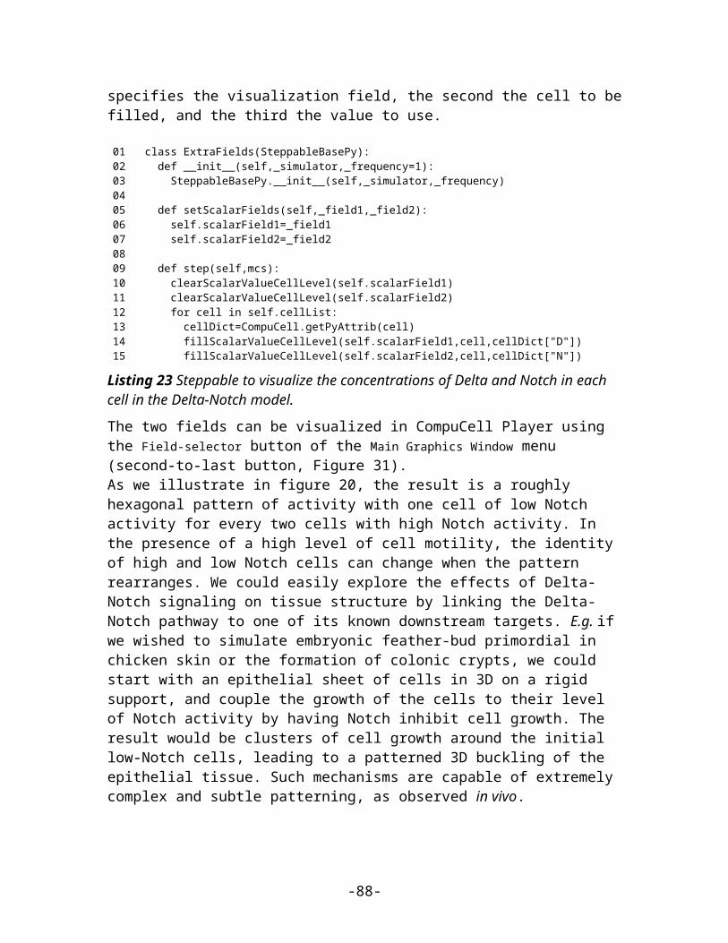
ContactMultiCad plugin is a modified version of ContactLocalProduct plugin. In this case users can use several cadherins and describe how they translate into contact energy.The energy formula used by this plugin is given below:
where indexes i, j label pixels, denotes contact energy between cell types
and , exactly as in “regular” contact plugin and indexes m,n label cadherins in cells composed f pixels i and j respectively.
The syntax for this plugin is as follows:
<Plugin Name="ContactMultiCad">
<Energy Type1="Medium" Type2="CadExpLevel1">0</Energy> <Energy Type1="Medium" Type2="CadExpLevel2">0</Energy> <Energy Type1="CadExpLevel1" Type2="CadExpLevel1">0</Energy> <Energy Type1="CadExpLevel1" Type2="CadExpLevel2">0</Energy> <Energy Type1="CadExpLevel2" Type2="CadExpLevel2">0</Energy>
<SpecificityCadherin> <Specificity Cadherin1="NCad1" Cadherin2="NCad1">-10</Specificity> <Specificity Cadherin1="NCad0" Cadherin2="NCad0">-12</Specificity> <Specificity Cadherin1="NCad1" Cadherin2="NCad0">-1</Specificity> </SpecificityCadherin>
<EnergyOffset>0.0</EnergyOffset> </NeighborOrder>2</NeighborOrder> </Plugin>
Entries of the type <Energy Type1="Medium" Type2="CadExpLevel1">0</Energy> have the same meaning as in “regular” contact energy. Specificity parameters
specification are enclosed between tags <SpecificityCadherin> and <SpecificityCadherin>. The names NCad0 and Ncad1 are arbitrary. However the
matrix will be ordered according to lexographic order of Cadherin names. For that reason we recommend that you name cadherins in such a way that makes it easy what the order will be. As in the example above using NameNumber(e.g. NCad0, NCad1) makes it easy to figure out what the order will be (NCad0 will get index 0 and NCad1 will get index 1). This is important because cadherins will be set in Python and if you won't keep track of the ordering of the specificity you might wrongly assign cadherins in Python and get unexpected results. In the example the order of cadherins is clear based on the definition of cadherin specificity parameters.
9.2.18 MolecularContactThis plugin is analogous to ContactLocalProduct and allows users to specify functional form of adhesion molecules interactions using Python syntax. It is in beta state and for
-88-
, 07/31/09,
?
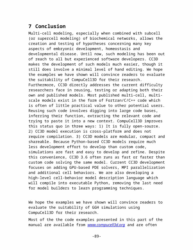
this reason we are not discussing it in more detail and currently suggest to use Either AdhesionFlex or ContactLocal product plugins.
9.2.19 ContactCompartmentThis plugin is a generalization of the contact energy plugin for the case of compartmental cell models.
where i and j denote pixels , denotes, as before, a cell type of a cell with cluster id and cell id. In compartmental cell models a cell is a collection of subcells. Each subcell has a unique id (cell id). In addition to that each subcell will have additional attribute, a cluster id that determines to which cluster of subcells a given subcell belongs. (think of a cluster as a cell with nonhomogenous cytoskeleton) The idea here is to have different contact energies between subcells belonging to the same cluster and different energies for cells belonging to different clusters. Technically subcells of a cluster are “regular” CompuCell3D cells. By giving them an extra attribute cluster id we can
introduce a concept of compartmental cells. In our convention 0,0) denotes medium
Introduction of cluster id and cell id are essential for the definition of
.
As you can see from above there are two hierarchies of contact energies – external and internal. The energies depend on cell types as in the case “regular” Contact plugin. Now, however, depending whether pixels for which we calculate contact energies belong to the same cluster or not we will use internal or external contact energies respectively.
-89-
=1
=2 =3
=4 =5 =6
=1
=2
Figure 20. Two compartmental cells (cluster id =1 and cluster id =2) Compartmentalized cell =1 consists of subcells with cell id =1,2,3 and compartmentalized cell =2 consists of subcells with cell id =4,5,6
, 07/31/09,
A annotated figure would make it more clear.

9.2.20 LengthConstraint Plugin
This plugin imposes elongation constraint on the cell. Effectively it “measures” a cell along its “axis of elongation” and ensures that cell length along the elongation axis is close to target length. For detailed description of this algorithm in 2D see Roeland Merks' paper “Cell elongation is a key to in silico replication of in vitro vasculogenesis and subsequent remodeling” Developmental Biology 289 (2006) 44-54). This plugin is usually used in conjunction with Connectivity Plugin or ConnectivityGlobal Plugin. The syntax is as follows:
<Plugin Name="LengthConstraint"> <LengthEnergyParameters CellType="Body1" TargetLength="30" LambdaLength="5"/></Plugin>
LambdaLength determines the degree of cell length oscillation around TargetLength parameter. The higher LambdaLength the less freedom a cell will have to deviate from TargetLength. In the 3D case we use the following syntax:
<Plugin Name="LengthConstraint"> <LengthEnergyParameters CellType="Body1" TargetLength="20" MinorTargetLength="5" LambdaLength="100" /></Plugin>
Notice new attribute called MinorTargetLength. In 3D it is not sufficient to constrain the "length" of the cell you also need to constrain "width" of the cell along axis perpendicular to the major axis of the cell. This "width" is referred to as MinorTargetLength.
The parameters are assigned using Python – see Demos\elongationFlexTest example.
To control length constraint individually for each cell we may use Python scripting to assign LambdaLength, TartgetLength and in 3D MinorTargetLength. In Python steppable we typically would write the following code:self.lengthConstraintPlugin.setLengthConstraintData(cell,10,20) which enables length constraint for cell cell with LambdaLength=10 and TargetLength=20. In 3D we may specify MinorTargetLength (we set it to 5) by adding 4th
parameter to the above call:self.lengthConstraintPlugin.setLengthConstraintData(cell,10,20,5)
If we use CC3DML specification of length constraint for certain cell types and in Python we set this constraint individually for a single cell then the local definition of the constraint has priority over definitions for the cell type.
If, in the simulation, we will be setting length constraint for only few individual cells then it is best to manipulate the constraint parameters from the Python script. In this case in
-90-

the CC3DML we only have to declare that we will use length constraint plugin and we may skip the definition by-type definitions:<Plugin Name="LengthConstraint"/>
Remark: When using target length plugins (either global , as shown here, or local as we will show in the subsequent subsection) it is important to use connectivity constraint. This constrain will check if a given pixel copy can break cell connectivity. If so, it will add large energy penalty (defined by a user) to change of energy effectively prohibiting such pixel copy. In the case of 2D on square lattice checking cell connectivity can be done locally and thus is very fast. Unfortunately on hex lattice and in 3D on either lattice we don’t have an algorithm of performing such check locally and therefore we do it globally using breadth first search algorithm and comparing volumes of cells calculated this way with actual volume of the cell. If they agree we conclude that cell connectivity is preserved. However the computational cost of running such algorithm, can be quite high. Therefore if one does need extremely elongated cells (it is when connectivity algorithm has to do a lot of work) one may neglect connectivity constraint and use Length constrain only. For slight cells elongations the connectivity should be preserved however, occasionally cells may fragment.
9.2.21 Connectivity PluginsThe basic Connectivity plugin works only in 2D and only on square lattice and is used to ensure that cells are connected or in other words to prevent separation of the cell into pieces. The detailed algorithm for this plugin is described in Roeland Merks' paper “Cell elongation is a key to in-silico replication of in vitro vasculogenesis and subsequent remodeling” Developmental Biology 289 (2006) 44-54). There was one modification of the algorithm as compared to the paper. Namely, to ensure proper connectivity we had to reject all spin flips that resulted in more that two collisions. (see the paper for detailed explanation what this means). The syntax of the plugin is straightforward:
<Plugin Name="Connectivity"> <Penalty>100000</Penalty> </Plugin>
Penalty denotes energy that will be added to overall change of energy if attempted spin flip would violate connectivity constraints. If the penalty is positive and much larger than the absolute value of other energy changes in the simulation this has the effect of preventing a spin flip from occurring.A more general type of connectivity constraint is implemented in ConnectivityGlobal plugin. In this case we calculate volume of a cell using breadth first search algorithm and compare it with actual volume of the cell. If they agree we conclude that cell connectivity is preserved. This plugin works both in 2D and 3D and on either type of lattice. However the computational cost of running such algorithm, can be quite high so it is best to limit this plugin to cell types for which connectivity of cell is really essential:
<Plugin Name="ConnectivityGlobal">
-91-
, 07/31/09,
?
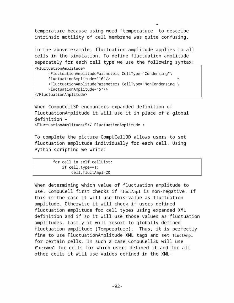
<Penalty Type="Body1">1000000000</Penalty></Plugin>
In certain types of simulation it may happen that at some point cells change cell types. If a cell that was not subject to connectivity constraint, changes type to the cell that is constrained by global connectivity and this cell is fragmented before type change this situation normally would result in simulation freeze. However CompuCell3D, first before applying constraint it will check if the cell is fragmented. If it is, there is no constraint. Global connectivity constraint is only applied when cell is non-fragmented. The numerical value of Penalty in the XML syntax above does not really matter as long as it is greater than 0. CompuCell3D guarantees that cells for which penalty is greater than 0 will remain connected.
Quite often in the simulation we don't need to impose connectivity constraint on all cells or on all cells of given type. Usually only select cell types or select cells are elongated and therefore need connectivity constraint. In such a case we use ConnectivityLocalFlex plugin and assign connectivity constraints to particular cells in Python
In XML we only declare: <Plugin Name="ConnectivityLocalFlex"/>
In Python we manipulate/access connectivity parameters for individual cells using the following syntax:
self.connectivityLocalFlexPlugin.setConnectivityStrength(cell,20.7)
self.connectivityLocalFlexPlugin.getConnectivityStrength(cell)
See also example in Demos\elongationLocalFlexTest.
ConnectivityLocalFlex plugin works only in 2D and on a square lattice. We may also use ConnectivityGlobal plugin to set connectivity constraint individually for each cell. Analogously, as in the case of ConnectivityLocalFlex , in the CC3DML we declare<Plugin Name="ConnectivityGlobal"/>and in Python we manipulate/access connectivity parameters for individual cells using the following syntax:self.connectivityGlobalPlugin.setConnectivityStrength(cell,10000000)
self.connectivityGlobalPlugin.getConnectivityStrength(cell)
9.2.22 Mitosis Plugin
-92-
Mitosis plugin carries out cell division into two cells once the parent cell reaches critical volume (DoublingVolume). The two cells after mitosis will have approximately the same volume although it cannot be guaranteed in general case if the parent cell is fragmented. One major problem with Mitosis plugin is that after mitosis the attributes of the offspring cell might not be initialized properly. By default cell type of the offspring cell will be the same as cell type of parent and they will also share target volume. All other parameters for the new cell remain uninitialized. Remark: For this reason we stringly recommend using Mitosis plugin through Python interface as there users can quite easily customize what happens to parent and offspring cells after mitosis. An example of the use of Mitosis plugin through Python scripting is provided in CompuCell3D’s Python Scripting Manual. The syntax of the “standard” mitosis plugin is the following:
<Plugin Name="Mitosis"> <DoublingVolume>50</DoublingVolume></Plugin>
Every time a cell reaches DoublingVolume it will undergo the mitosis and the offspring cell will inherit type and target volume of the parent. If this simple behavior is unsatisfactory consider use Python scripting to implement proper mitotic divisions of cells.
9.2.23 Secretion PluginIn earlier version os of CC3D secretion was part of PDE solvers. We still support this mode of model description however, starting in 3.5.0 we developed separate plugin which handles secretion only. Via secretion plugin we can simulate cell ular secretion of various chemicals. The secretion plugin allows users to specify various secretion modes in the XML file - XML syntax is practically identical to the SecretionData syntax of PDE solvers. In addition to this Secretion plugin allows users to maniupulate secretion properties of individual cells from Python level. To account for possibility of PDE solver being called multiple times during each MCS, the Secretion plugin can be called multiple times in each MCS as well. We leave it up to user the rescaling of secretion constants when using multiple secretion calls in each MCS. Note:Secretion for individual cells invoked via Python will be called only once per MCS.
Typical XML xyntax for Secretion plugin is presented below:
<Plugin Name="Secretion"> <Field Name="ATTR" ExtraTimesPerMC=”2”> <Secretion Type="Bacterium">200</Secretion> <SecretionOnContact Type="Medium" SecreteOnContactWith="B">300</SecretionOnContact> <ConstantConcentration Type="Bacterium">500</ConstantConcentration> </Field></Plugin>
By default ExtraTimesPerMC is set to 0 - meaning no extra calls to Secretion plugin per MCS.
Typical use of secretion from Python is dempnstrated best in the example below:
-93-
, 07/31/09,
In case of uneven volume distribution between daughter cells, since target volume of daughter cells are the same, within few MCS, they will adapt their volume to the target volume.

class SecretionSteppable(SecretionBasePy): def __init__(self,_simulator,_frequency=1): SecretionBasePy.__init__(self,_simulator, _frequency) def step(self,mcs): attrSecretor=self.getFieldSecretor("ATTR") for cell in self.cellList: if cell.type==3: attrSecretor.secreteInsideCell(cell,300) attrSecretor.secreteInsideCellAtBoundary(cell,300) attrSecretor.secreteOutsideCellAtBoundary(cell,500) attrSecretor.secreteInsideCellAtCOM(cell,300)Remark: Instead of using SteppableBasePy class we are using SecretionBasePy class. The reason for this is that in order for secretion plugin with secretion modes accessible from Python to behave exactly as previous versions of PDE solvers (where secretion was done first followed by “diffusion” step) we have to ensure that secretion steppable implemented in Python is called before each Monte Carlo Step, which implies that it will be also called before “diffusing” function of the PDE solvers. SecretionBasePy sets extra flag which ensures that steppable which inherits from SecretionBasePy is called before MCS (and before all “regular’ Python steppables). There is no magic to SecretionBasePy - if you still want to use SteppableBasePy as a base class for secretion (or for that matter SteppablePy) do so, but remember that you need to set flag:
self.runBeforeMCS=1
to ensure that your new stoppable will run before each MCS. See example below for alternative implementation of SecretionSteppable using SteppableBasePy as a base class:
class SecretionSteppable(SteppableBasePy): def __init__(self,_simulator,_frequency=1): SteppableBasePy.__init__(self,_simulator, _frequency) self.runBeforeMCS=1 def step(self,mcs): attrSecretor=self.getFieldSecretor("ATTR") for cell in self.cellList: if cell.type==3: attrSecretor.secreteInsideCell(cell,300) attrSecretor.secreteInsideCellAtBoundary(cell,300) attrSecretor.secreteOutsideCellAtBoundary(cell,500) attrSecretor.secreteInsideCellAtCOM(cell,300)
The secretion of individual cells is handled through Field Secretor objects. Field Secretor concenpt is quite convenient because the amoun of Python coding is quite small. To secrete chemical (this is now done for individual cell) we first create field secretor object, attrSecretor=self.getFieldSecretor("ATTR"), which allows us to secrete into field called ATTR.
-94-
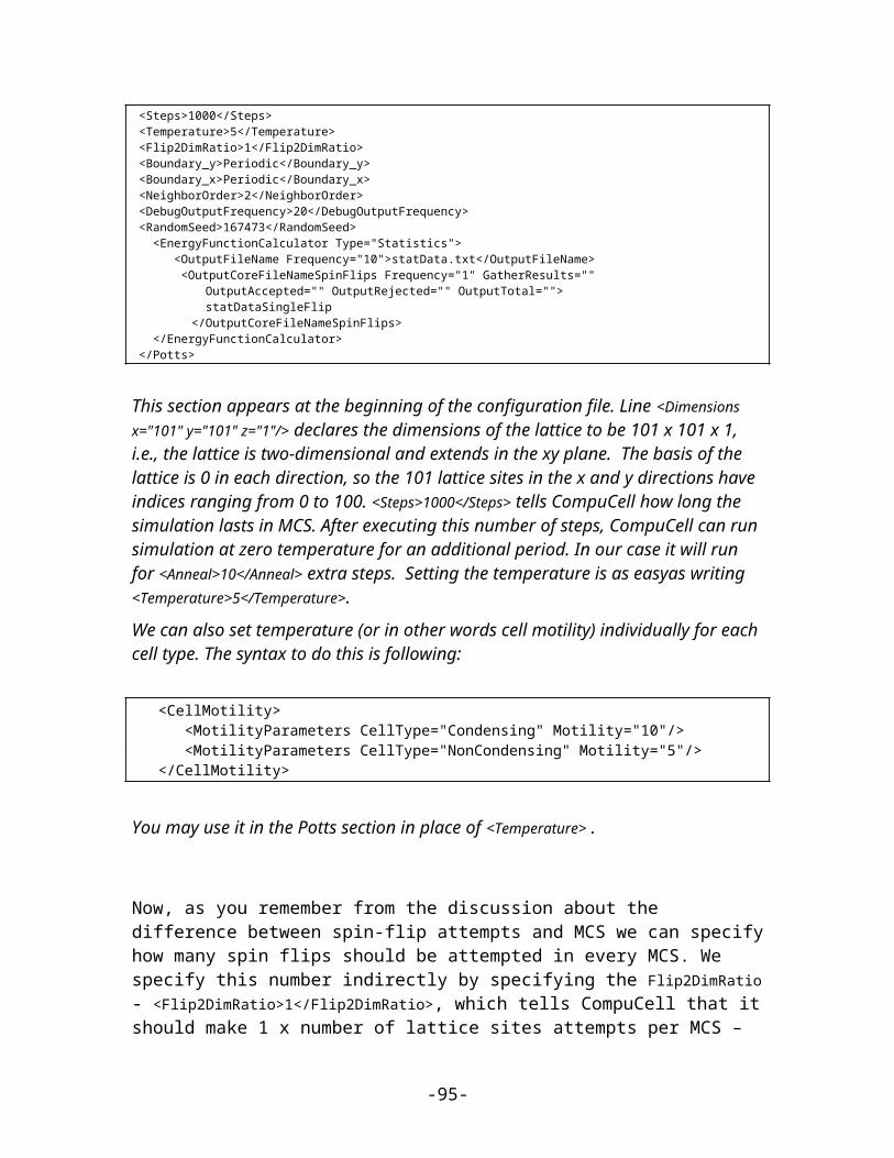
Remark: Make sure that fields into which you will be secreting chemicals exist. They are usually fields defined in PDE solvers. When using secretion plugin you do not need to specify SecretionData section for the PDE solversThen we pick a cell and using field secretor we simulate secretion of chemical ATTR by a cell:
attrSecretor.secreteInsideCell(cell,300)
Currently we support 4 secretion modes for individual cells:1. secreteInsideCell – this is equivalent to secretion in every pixel belonging to a
cell2. secreteInsideCellAtBoundary – secretion takes place in the pixels belonging
to the cell boundary 3. secreteInsideCellAtBoundary – secretion takes place in pixels which are
outide the cell but in contact with cell boundary pixels4. secreteInsideCellAtCOM – secretion at the center of mass of the cell
As you may infer from above modes 1, 2 and 3 require tracking of pixels belonging to cell and pixels belonging to cell boundary. If you are not using modes 1-3 you may disable pipxel tracking by including <DisablePixelTracker/> and/or <DisableBoundaryPixelTracker/> tags – as shown in the example below:<Plugin Name="Secretion">
<DisablePixelTracker/> <DisableBoundaryPixelTracker/>
<Field Name="ATTR" ExtraTimesPerMC=”2”> <Secretion Type="Bacterium">200</Secretion> <SecretionOnContact Type="Medium" SecreteOnContactWith="B">300</SecretionOnContact> <ConstantConcentration Type="Bacterium">500</ConstantConcentration> </Field></Plugin>
9.2.24 . PDESolverCaller Plugin
PDE solvers in CompuCell3D are implemented as steppables . This means that by default they are called every MCS. In many cases this is insufficient. For example if diffusion constant is large, then explicit finite difference method will become unstable and the numerical solution will have no sense. To fix this problem one could call PDE solver many times during single MCS. This is precisely the task taken care of by PDESolverCaller plugin. The syntax is straightforward:
<Plugin Name="PDESolverCaller"> <CallPDE PDESolverName="FlexibleDiffusionSolverFE"ExtraTimesPerMC="8"/></Plugin>
-95-

All you need to do is to give the name of the steppable that implements a given PDE solver and pass let CompCell3D know how many extra times per MCS this solver is to be called (here FlexibleDiffusionSolverFE was 8 extra times per MCS).
9.2.25 Elasticity Plugin and ElasticityTracker Plugin
This plugin is responsible for handling the following energy term:
where is a distance between center of masses of cells i and j and is a target length
corresponding to .The syntax of this plugin is the following
<Plugin Name="ElasticityEnergy"> <LambdaElasticity>200.0</LambdaElasticity> <TargetLengthElasticity>6</TargetLengthElasticity> </Plugin>
In this case and are the same for all participating cells types.By adding extra attribute <Local/> to the above plugin:
<Plugin Name="ElasticityEnergy"> <Local/> <LambdaElasticity>200.0</LambdaElasticity> <TargetLengthElasticity>6</TargetLengthElasticity> </Plugin>
we tell CompuCell3D to use and defined on per pair of cells basis. The
initialization of and usually takes place in Python script and users must make sure
that and or else one can get unexpected results. We provide example python and xml files that demo the use of plasticity plugin.
Users have to specify which cell types participate in the plasticity calculations. This is done by including ElasticityTracker plugin before Elasticity plugin in the xml file. The syntax is very clear:
<Plugin Name="ElasticityTracker"> <IncludeType>Body1</IncludeType> <IncludeType>Body2</IncludeType> <IncludeType>Body3</IncludeType> </Plugin>
All is required is a list of participating cell types. Here cells of type Body1, Body2 and Body3 will be taken into account for elasticity energy calculation purposes.
-96-
, 07/31/09,
Example?

The way in which CompuCell3D determines which cells are to be included in the elasticity energy calculations is by examining which cells are in contact with each other before simulation begins. If the types of cells touching each other are listed in the list of IncudeTypes of ElasticityTracker then such cells are being taken into account when calculating elastic constraint. Cells which initially are not touching will not participate in calculations even if their type is included in the list of “ElasticityTracker”. However, in some cases it is desirable to add elasticity pair even for cells that do not touch each other or do it once simulation has started. To do this ElasticityTracker plugin defines two function :
assignElasticityPair(_cell1 , _cell2)
removeElasticityPair(_cell1 , _cell2)
where _cell1 and _cell2 denote pointers to cell objects. These functions add or remove two cell links to or from elastic constraint. Typically they are called from Python level.
9.2.26 FocalPointPlasticity PluginSimilarly as Elasticity plugin, FocalPointPlasticity pust constrains the distance between cells’ center of masses. The main difference is that the list of “focal point plasticity neighbors” can change as the simulation goes and user specifies the maximum number of “focal point plasticity neighbors” a given cell can have. Let’s look at relatively simple XML syntax of FocalPointPlasticityPlugin (see Demos/FocalPointPlasticity example and we will show more complex examples later):
<Plugin Name="FocalPointPlasticity"> <Parameters Type1="Condensing" Type2="NonCondensing"> <Lambda>10.0</Lambda> <ActivationEnergy>-50.0</ActivationEnergy> <TargetDistance>7</TargetDistance> <MaxDistance>20.0</MaxDistance> <MaxNumberOfJunctions>2</MaxNumberOfJunctions> </Parameters>
<Parameters Type1="Condensing" Type2="Condensing"> <Lambda>10.0</Lambda> <ActivationEnergy>-50.0</ActivationEnergy> <TargetDistance>7</TargetDistance> <MaxDistance>20.0</MaxDistance> <MaxNumberOfJunctions>2</MaxNumberOfJunctions> </Parameters> <NeighborOrder>1</NeighborOrder> </Plugin>
Parameters section describes properties of links between cells. MaxNumberOfJunctions, ActivationEnergy, MaxDistance and NeighborOrder are responsible for establishing
-97-
, 07/31/09,
Cell which initially are not touching will not participate in this plug even if their type is included in the list of “ElasticityTracker”.
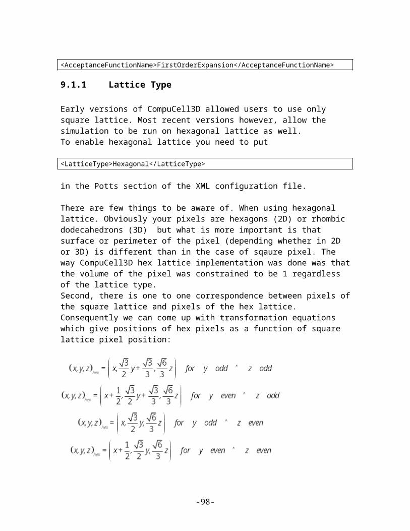
connections between cells. CC3D constantly monitors pixel copies and during pixel copy between two neighboring cells/subcells it checks if those cells are already participating in focal point plasticity constraint. If they are not, CC3D will check if connection can be made (e.g. Condensing cells can have up to two connections with Condensing cells and up to 2 connections with NonCondensing cells – see first line of Parameters section and MaxNumberOfJunctions tag). The NeighborOrder parameter determines the pixel vicinity of the pixel that is about to be overwritten which CC3D will scan in search of the new link between cells. NeighborOrder 1 (which is default value if you do not specify this parameter) means that only nearest pixel neighbors will be visited. The ActivationEnergy parameter is added to overall energy in order to increase the odds of pixel copy which would lead to new connection.
Once cells are linked the energy calculation is carried out in a very similar way as for the Elasticity plugin:
where is a distance between center of masses of cells i and j and is a target length
corresponding to .ij and Lij between different cell types are determined using Lambda and TargetDistance tags. The MaxDistance determines the distance between cells’ center of masses when the link between those cells break. When the link breaks, then in order for the two cells to reconnect they would need to come in contact (in order to reconnect). However it is usually more likely that there will be other cells in the vicinity of separated cells so it is more likely to establish new link than restore broken one.The above example was one of the simplest examples of use of FocalPointPlasticity. A more complicated one involves compartmental cells. In this case each cell has separate “internal” list of links between cells belonging to the same cluster and another list between cells belonging to different clusters. The energy contributions from both lists are summed up and everything that we have said when discussing example above applies to compartmental cells. Sample syntax of the FocalPointPlasticity plugin which includes compartmental cells is shown below. We use InternalParameters tag/section to describe links between cells of the same cluster (see Demos/FocalPointPlasticity example):
<Plugin Name="FocalPointPlasticity"> <Parameters Type1="Top" Type2="Top"> <Lambda>10.0</Lambda> <ActivationEnergy>-50.0</ActivationEnergy> <TargetDistance>7</TargetDistance> <MaxDistance>20.0</MaxDistance> <MaxNumberOfJunctions NeighborOrder="1">1</MaxNumberOfJunctions> </Parameters>
<Parameters Type1="Bottom" Type2="Bottom">
-98-

<Lambda>10.0</Lambda> <ActivationEnergy>-50.0</ActivationEnergy> <TargetDistance>7</TargetDistance> <MaxDistance>20.0</MaxDistance> <MaxNumberOfJunctions NeighborOrder="1">1</MaxNumberOfJunctions> </Parameters> <InternalParameters Type1="Top" Type2="Center"> <Lambda>10.0</Lambda> <ActivationEnergy>-50.0</ActivationEnergy> <TargetDistance>7</TargetDistance> <MaxDistance>20.0</MaxDistance> <MaxNumberOfJunctions>1</MaxNumberOfJunctions> </InternalParameters>
<InternalParameters Type1="Bottom" Type2="Center"> <Lambda>10.0</Lambda> <ActivationEnergy>-50.0</ActivationEnergy> <TargetDistance>7</TargetDistance> <MaxDistance>20.0</MaxDistance> <MaxNumberOfJunctions>1</MaxNumberOfJunctions> </InternalParameters> <NeighborOrder>1</NeighborOrder> </Plugin>
Sometimes it is necessary to modify link parameters individually for every cell pair. In this case we would manipulate FocalPointPlasticity links using Python scripting. Example Demos/FocalPointPlasticityCompartments demonstrates exactly this situation. Still, you need to include XML section as the one shown above for compartmental cells, because we need to tell CC3D how to link cells. The only notable difference is that in the XML we have to include <Local/> tag to signal that we will set link parameters (Lambda, TaretDistance, MaxDistance) individually for each cell pair:
<Plugin Name="FocalPointPlasticity"> <Local/> <Parameters Type1="Top" Type2="Top"> <Lambda>10.0</Lambda> <ActivationEnergy>-50.0</ActivationEnergy> <TargetDistance>7</TargetDistance> <MaxDistance>20.0</MaxDistance> <MaxNumberOfJunctions NeighborOrder="1">1</MaxNumberOfJunctions> </Parameters> ……..</Plugin>
Python steppable where we manipulate cell-cell focal point plasticity link properties is shown below:
class FocalPointPlasticityCompartmentsParams(SteppablePy): def __init__(self,_simulator,_frequency=10):
-99-

SteppablePy.__init__(self,_frequency) self.simulator=_simulator self.focalPointPlasticityPlugin=CompuCell.\ getFocalPointPlasticityPlugin() self.inventory=self.simulator.getPotts().\ getCellInventory() self.cellList=CellList(self.inventory)
def step(self,mcs): for cell in self.cellList: for fppd in InternalFocalPointPlasticityDataList\ (self.focalPointPlasticityPlugin,cell): self.focalPointPlasticityPlugin.\ setInternalFocalPointPlasticityParameters\ (cell,fppd.neighborAddress,0.0,0.0,0.0)
The syntax to change focal point plasticity parameters (or as here internal parameters) is as follows:setFocalPointPlasticityParameters(cell1, cell2, lambda,\ targetDistance, maxDistance)
setInternalFocalPointPlasticityParameters(cell1, cell2, lambda,\ targetDistance, maxDistance)
Similarly to inspect current values of the focal point plasticity parameters we would use the following Python construct:
for cell in self.cellList: for fppd in InternalFocalPointPlasticityDataList\ (self.focalPointPlasticityPlugin,cell): print "fppd.neighborId",fppd.neighborAddress.id " lambda=",fppd.lambdaDistance
For non-internal parameters we simply use FocalPointPlasticityDataList instead of InternalFocalPointPlasticityDataList .
Examples Demos/FocalPointPlasticity… show in relatively simple way how to use FocalPointPlasticity plugin. Those examples also contain useful comments.
When using FocalPointPlasticity Plugin from mitosis module one might need to break or create focal point plasticity links. To do so FocalPointPlasticity Plugin provides 4 convenience functions which can be invoked from the Python level:
deleteFocalPointPlasticityLink(cell1,cell2)
deleteInternalFocalPointPlasticityLink(cell1,cell2)
createFocalPointPlasticityLink(\cell1,cell2,lambda,targetDistance,maxDistance)
createInternalFocalPointPlasticityLink(\
-100-
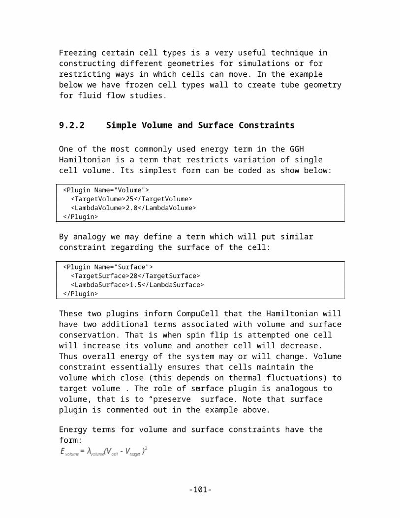
cell1,cell2,lambda,targetDistance,maxDistance)
9.2.27 Curvature PluginThis plugin implements energy term for compartmental cells. It is based on “A New Mechanism for Collective Migration in Myxococcus xanthus”, J. Starruß, Th. Bley, L. Søgaard-Andersen and A. Deutsch, Journal of Statistical Physics, DOI: 10.1007/s10955-007-9298-9, (2007). For a “long” compartmental cell composed of many subcells it imposes constraint on curvature of cells. The syntax is slightly complex:
<Plugin Name="Curvature"> <InternalParameters Type1="Top" Type2="Center"> <Lambda>100.0</Lambda> <ActivationEnergy>-50.0</ActivationEnergy> </InternalParameters>
<InternalParameters Type1="Center" Type2="Center"> <Lambda>100.0</Lambda> <ActivationEnergy>-50.0</ActivationEnergy> </InternalParameters> <InternalParameters Type1="Bottom" Type2="Center"> <Lambda>100.0</Lambda> <ActivationEnergy>-50.0</ActivationEnergy> </InternalParameters>
<InternalTypeSpecificParameters> <Parameters TypeName="Top" MaxNumberOfJunctions="1" NeighborOrder="1"/> <Parameters TypeName="Center" MaxNumberOfJunctions="2" NeighborOrder="1"/> <Parameters TypeName="Bottom" MaxNumberOfJunctions="1" NeighborOrder="1"/> </InternalTypeSpecificParameters>
</Plugin>
The InternalTypeSpecificParameter tells Curvature Plugin how many neighbors a cell of given type will have. In this case, numbers which make sense are 1 and 2. The middle segment will have 2 connection and head and tail segments will have only one connection with neighboring segmens (subcells). The connections are established dymamically. The way it happens is that during simulation CC3D constantly monitors pixel copies and during pixel copy between two neighboring cells/subcells it checks if those cells are already “connected” using curvature constraint. If they are not, CC3D will check if connection can be made (e.g. Center cells can have up to two connections and Top and Bottom only one connection). Usually establishing connections takes place at the beginning if the simulation and often happens within first Monte Carlo Step (depending
-101-
on actual initial configuration, of course, but if segments touch each other connections are established almost immediately). The ActivationEnergy parameter is added to overall energy in order to increase the odds of pixel copy which would lead to new connection. Lambda tag/parameter determines “the strength” of curvature constraint. The higher the Lambda the more “stiff” cells will be i.e. they will tend to align along straight line.
9.2.28 PlayerSettings Plugin
This plugin allows users to specify or configure Player settings directly from XML, without s single click. Some users might prefer this way of setting configuring Player. In addition to this if users want to run two different simulations at the same time on the same machine but with different , say, cell colors, then doing it with “regular” Player configuration file might be tricky. The solution is to use PlayerSetting Plugin. The syntax of this plugin is as follows:
<Plugin Name="PlayerSettings"> <Project2D XZProj="50"/> <Concentration LegendEnable="true" NumberOfLegendBoxes="3"/> <VisualControl ScreenshotFrequency="200" ScreenUpdateFrequency="10" NoOutput="true" ClosePlayerAfterSimulationDone="true" /> <Border BorderColor="red" BorderOn="false"/> <TypesInvisibleIn3D Types="0,2,4,5"/> <Cell Type="1" Color="red"/> <Cell Type="2" Color="yellow"/> <!-- Note: SaveSettings flag is unimportant for the new Player because whenever settings are changed from XML script they are written by default to disk This seems to be default behavior of most modern applications. We may implement this feature later <Settings SaveSettings="false"/> --></Plugin>
As can be seen from above syntax all the keywords correspond to an action in the Player.Project2D sets up the values of the projection on the Player steering bar. Here we set the player to start 2D display in the xz projection with y coordinate set to 50. Borders and contours properties are handled using Border and Contour elements. Specifying cell colors is done using Cell element. VisualControl element allows users to specify zoom factor and screen update and screenshot frequencies. Notice, screen update frequency migh not work properly when using Python script. In this case CompuCell will use whatever screen update frequency was stored in the config file (by default 1). We may also change things such as screen update frequency or screenshot frequency and choose whether or not to close the player after the simulation.To start Player in the 3D view instead of adding <Project2D> tag we add <View3D> section:
-102-
, 07/31/09,
Not clear?
<View3D> <CameraClippingRange Max="388.363853764" Min="182.272762471"/> <CameraFocalPoint x="50.0" y="50.0" z="0.75"/> <CameraPosition x="150.062764552" y="-88.9777652942" z="213.639720537"/> <CameraViewUp x="0.112255891114" y="0.855400655565" z="0.505656339196"/> </View3D>
The camera settings stored here position 3D camera. The best way to get those settings is to run a simulation, add 2D screenshot using camera button, switch to 3D and position camera (using mouse) however you like and subsequently add another screenshot using camera button, save screenshot descrition file (File->Save Screenshot Description…) and open up in text editor newly saved screenshot description file (with .sdfml extension) and copy camera setting from there into PlayerSettings <View3D> section. An example of using Player settings is shown in Demos\cellsort_2D\cellsort_2D_PlayerSettings.xml.Although the set of allowed changes of player settings is fairly small at the moment we believe that the options that users have right now are quite sufficient for configuring the Player from the XML or python level. We will continue adding new options though.
9.2.29 BoundaryPixelTracker PluginThis plugin allows storing list of boundary pixels for each cell. The syntax is as follows:
<Plugin Name="BoundaryPixelTracker"> <NeighborOrder>1</NeighborOrder> </Plugin>
This plugin is also used by other plugins as a helper module.
9.2.30 GlobalBoundaryPixelTracker
This plugin tracks boundary pixels of all the cells including medium It is used in a Boundary Walker algorithm where instead of blindly picking pixel copy candidate we pick it from the set of pixels comprising boundaries of non frozen cells. In situations when lattice is large and there are not that many cells it makes sense to use BoundaryWalker algorithm to limit number of "wrong" pixel picks when perfming pixel copy attempts. Take a look at the following example:<Potts> <Dimensions x="100" y="100" z="1"/> <Anneal>10</Anneal> <Steps>10000</Steps> <Temperature>5</Temperature> <Flip2DimRatio>1</Flip2DimRatio> <NeighborOrder>2</NeighborOrder> <MetropolisAlgorithm>BoundaryWalker</MetropolisAlgorithm> <Boundary_x>Periodic</Boundary_x> </Potts>
<Plugin Name="GlobalBoundaryPixelTracker"> <NeighborOrder>2</NeighborOrder> </Plugin>
-103-
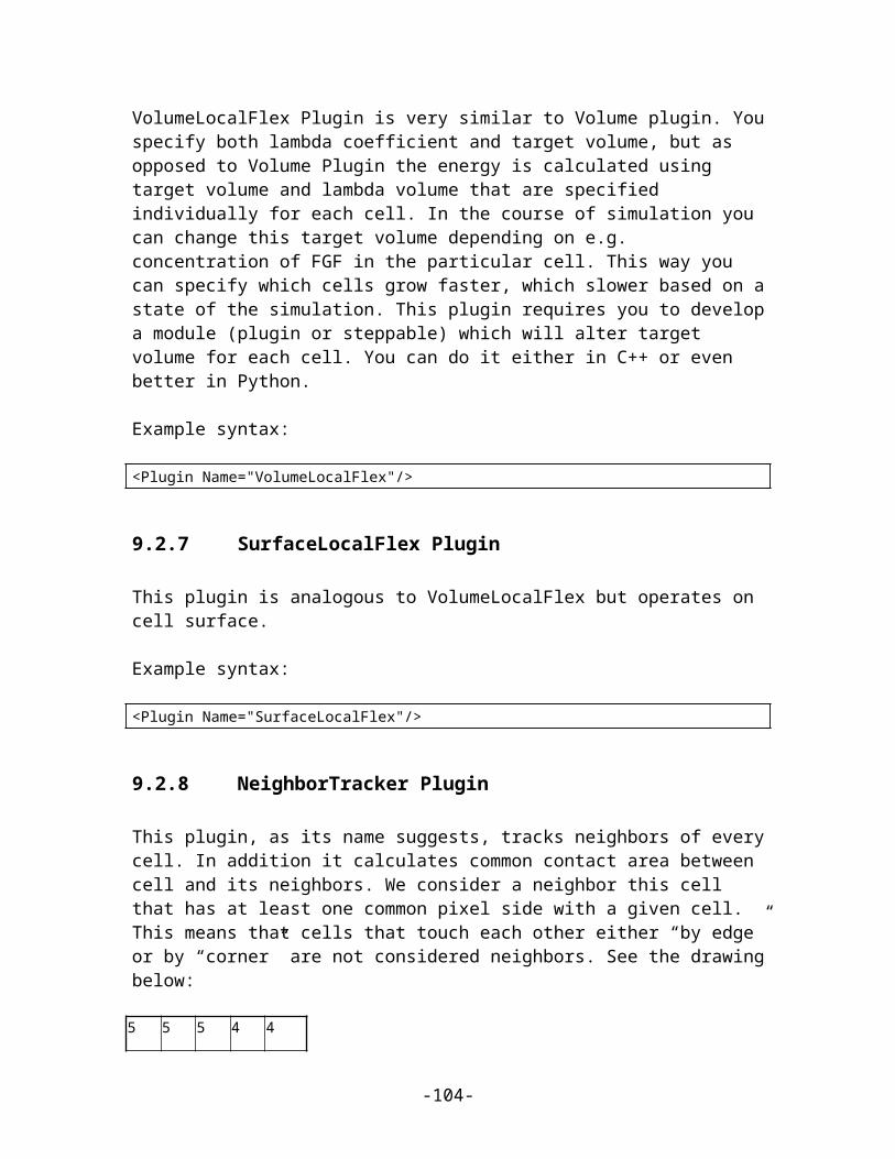
Here we are using BoundaryWalker algorithm (Potts section) and subsequently we list GlobalBoundaryTracker plugin where we set neighbor order to match that in the Potts section. The neighbor order determines how "thick" the overall boundary of cells will be. The higher this number the more pixels will belong to the boundary.
9.2.31 PixelTracker PluginThis plugin allows storing list of all pixels belonging to a given cell. The syntax is as follows:
<Plugin Name="PixelTracker"/>
This plugin is also used by other plugins (e.g. Mitosis) as a helper module.
9.2.32 MomentOfInertia PluginThis plugin updates tensor of inertia for every cell. Internally it uses parallel axis theorem to calculate most up-to-date tensor of inertia. It can be called directly:
<Plugin Name="MomentOfInertia"/>
However, most commonly it is called indirectly by other plugins like Elongation plugin.
MomentOfInertia plugin gives users access (via Python scripting) to current lengths of cell’s semiaxes. Examples in Demos/MomentOfInertia demonstrate how to get lengths of semiaxes:
axes=self.momentOfInertiaPlugin.getSemiaxes(cell)
axes is a 3-component vector with 0th element being length of minor axis, 1st – length of median axis (which is set to 0 in 2D) and 2nd element indicating the length of major semiaxis. Important: Because calculating lengths of semiaxes involves quite a few of floating point operations it may happen (usually on hexagonal lattice) that for cells composed of 1, 2, or 3 pixels one moment the square of one of the semiaxes may end up being slightly negative leadind to NaN (not a number)length. This is due to roundoff error and whenever CC3D detects very small absolute value of square of the length of semiaxes (10-6) it sets length of this semiaxes to 0.0 regardless whether the squared value is positive or negative. However it is a good practice to test whether the length of semiaxis is sane by doing simple if (here we show how to test for a NaN)
jf length!=length:print “length is NaN”:
else:print “length is a proper floating point number”
-104-
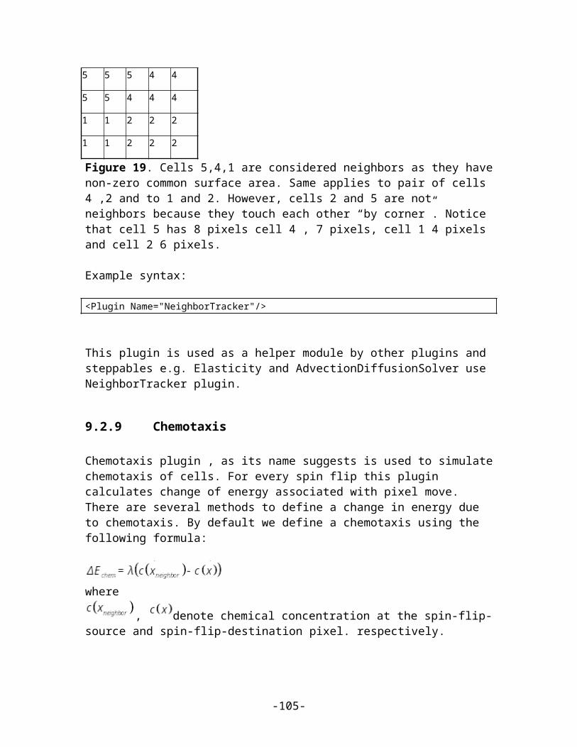
9.2.33 SimpleClock pluginThis plugin adds an integer as a cell attribute:
<Plugin Name="SimpleClock"/>
9.2.34 ConvergentExtension pluginThis is very specialized plugin which currently is in Tier 2 plugins in terms of support. IT implements energy term described in “Simulating Convergent Extension by Way of Anisotropic Differemtial Adhesion,” Zajac M, Jones GL, and Glazier JA, Journal of Theoretical Biology 222 (2), 2003.
CC3D’s ConvergentExtension plugin is a somewhat simplified version of energy term described in the paper.
This plugin uses the following syntax:
<Plugin Name="ConvergentExtension"> <Alpha Type="Condensing" >0.99</Alpha> <Alpha Type="NonCondensing" >0.99</Alpha> <NeighborOrder>2</NeighborOrder> </Plugin>
The Alpha tag represents numerical value of parameter from the paper.
9.3 Steppable SectionSteppables are CompuCell modules that are called every Monte Carlo Step (MCS). More precisely, they are called after all the spin attempts in a given MCS have been carried out. Steppables may have various functions like for example solving PDE's, checking if critical concentration threshold have been met, updating target volume or target surface given the concentration of come growth factor, initializing cell field, writing numerical results to a file etc. In summary Steppables perform all functions that need to be done every MCS. In the reminder of this section we will present steppables currently available in the CompuCell and describe their usage.
9.3.1 UniformInitializer Steppable
This steppable lays out pattern of cells on the lattice. It allows users to specify rectangular regions of field with square (or cube in 3D) cells of user defined types (or random types). Cells can be touching each other or can be separated by a gap.
The syntax of the plugin is as follows:
<Steppable Type="UniformInitializer"> <Region> <BoxMin x="35" y="0" z="30"/>
-105-
<BoxMax x="135" y="1" z="430"/> <Gap>0</Gap> <Width>5</Width> <Types>psm</Types> </Region></Steppable>
Above we have defined a 2D rectangular box filled with 5x5 cells touching each other (Gap=0) and having type psm. Notice that if you want to initialize 2D box in xz plane as above then y_min and y_max have to be 0 and 1 respectively.
Users can include as many regions as they want. The regions can overlap each other. Simply cells that are overwritten will either disappear or be truncated.
Additionally users can initialize region with random cell types chosen from provided list of cell types:
<Steppable Type="UniformInitializer"> <Region> <BoxMin x="35" y="0" z="30"/> <BoxMax x="135" y="1" z="430"/> <Gap>0</Gap> <Width>5</Width> <Types>psm,ncad,ncam</Types> </Region></Steppable>
When user specifies more than one cell type between <Types> tags (notice, the types have to be separated with ',' and there should be no spaces) then cells for this region will be initialized with types chosen randomly from the provided list (here the choices would be psm, ncad, ncam).Remark: If one of the type names is repeated inside <Types> element this type will get greater weighting means probability of assigning this type to a cell will be greater. So for example <Types>psm,ncad,ncam,ncam,ncam</Types> ncam will assigned to a cell with probability 3/5 and psm and ncad with probability 1/5.
9.3.2 BlobInitializer SteppableThis steppable is used to lay out circular blob of cells on the lattice. This plugin does not have yet the flexibility of UniformInitializer but this will change in the future release. Original syntax of this plugin looks as follows:
<Steppable Type="BlobInitializer"> <Gap>0</Gap> <Width>5</Width> <CellSortInit>yes</CellSortInit> <Radius>40</Radius> </Steppable>
-106-

The blob is centered in the middle of th lattice and has radius given by <Radius> parameter all cells are initially squares (or cubes in 3D) - <Width> determines the length of the cube or square side and <Gap> determines space between squares or cubes. <CellSortInit> tag and value yes is used to initialize cells randomly with type id being either 1 or 2. Otherwise all cells will have type id 1. This can be easily modified in Python . The most recent syntax for this plugin gives users additional flexibility in initializing cell field using BlobFieldInitializer:
<Steppable Type="BlobInitializer"> <Region> <Gap>0</Gap> <Width>5</Width> <Radius>40</Radius> <Center x="100" y="100" z="0"/> <Types>Condensing,NonCondensing</Types> </Region></Steppable Type="BlobInitializer">
Similarly as for the UniformFieldInitializer users can define many regions each of which is a blob of a particular center point , radius and list of cell types that will be assigned to cells forming the blob.
9.3.3 PIF InitializerTo initialize the configuration of the simulation lattice you can can write your own lattice initialization file. Our experience suggests that you will probably have to write your own initialization files rather than relying on built-in initializers. The reason is simple: the built-in initializers implement very simple cell layouts, and if you want to study more complicated cell arrangements, the built-in initializers will not be very helpful. Therefore we encourage you to learn how to prepare lattice initialization files. Again, file definition is not complicated and we will explain every step. The lattice initialization file tells CompuCell3D how to lay out assign the simulation lattice pixels to cells.
The Potts Initial File (PIF) is a simple file format that we created for easy specification of initial cell positions. The PIF consists of multiple lines of the following format:
cell# celltype x1 x2 y1 y2 z1 z2
Where cell# is the unique integer index of a cell, celltype is a string representing the cell's initial type, and x1 and x2 specify a range of x-coordinates contained in the cell (similarly y1 and y2 specify a range of y-coordinates and z1 and z2 specify a range of z-coordinates). Thus each line assigns a rectangular volume to a cell. If a cell is not perfectly rectangular, multiple lines can be used to build up the cell out of rectangular sub-volumes (just by reusing the cell# and celltype).
A PIF can be provided to CompuCell3D by including the steppable object PIFInitializer.
Let's look at a PIF example for foams:
-107-
0 Medium 0 101 0 101 0 0 1 Foam 13 25 0 5 0 0 2 Foam 25 39 0 5 0 0 3 Foam 39 46 0 5 0 0 4 Foam 46 57 0 5 0 0 5 Foam 57 65 0 5 0 0 6 Foam 65 76 0 5 0 0 7 Foam 76 89 0 5 0 0
These lines define a background of Medium which fills the whole lattice and is then overwritten by seven rectangular cells of type Foam numbered 1 through 7. Notice that these cells lie in the xy plane (z1=0 z2=0 implies that cells have thickness =1) so this example is a two-dimensional initialization.
You can write the PIF file manually, but using a script or program that will write PIF file for you in the language of your choice (Perl, Python, Matlab, Mathematica, C, C++, Java or any other programming language) will save a great deal of typing. You may also use tools like PIFTracer which allow you to "paint" the lattice by tracing regions of the experimental pictures.
Notice, that for compartmental cell model the format of the PIF file is different:
Include Clusterscluster # cell# celltype x1 x2 y1 y2 z1 z2
For example:
Include Clusters1 1 Side1 23 25 47 56 10 141 2 Center 26 30 50 54 10 141 3 Side2 31 33 47 56 10 141 4 Top 26 30 55 59 10 141 5 Bottom 26 30 45 49 10 142 6 Side1 35 37 47 56 10 142 7 Center 38 42 50 54 10 142 8 Side2 43 45 47 56 10 142 9 Top 38 42 55 59 10 142 10 Bottom 38 42 45 49 10 14
9.3.4 PIFDumper SteppableThis steppable does opposite to PIFIitializer – it writes PIF file of current lattice configuration. The syntax similar to the syntax of PIFInitializer:
<Steppable Type="PIFDumper" Frequency=”100”> <PIFName>line</PIFName></Steppable>
Notice that we used Frequency attribute of steppable to ensure that PIF files are written every 100 MCS. Without it they would be written every MCS. The file names will have the following format:
-108-

PIFName.MCS.pif
In our case they would be line.0.pif, line.100.pif, line.200.pif etc...
This plugin is actually quite useful. For example, if we want to start simulation from a more configuration of cells (not rectangular cells as this is the case when we use Uniform or Blob initializers). In such a case we would run a simulation with a PIFDumper included and once the cell configuration reaches desired shape we would stop and use PIF file corresponding to this state. Once we have PIF initial configuration we may run many simulation starting from the same, realistic initial condition.
9.3.5 Mitosis Steppabe.This steppable is described in great detail in Python tutorial but because of its importance we are including a copy of that description here.In developmental simulations we often need to simulate cells which grow and divide. In earlier versions of CompuCell3D we had to write quite complicated plugin to do that which was quite cumbersome and unintuitive (see example 9). The only advantage of the plugin was that exactly after the pixel copy which had triggered mitosis condition CompuCell3D called cell division function immediately. This guaranteed that any cell which was supposed divide at any instance in the simulation, actually did. However, because state of the simulation is normally observed after completion of full a Monte Carlo Step, and not in the middle of MCS it makes actually more sense to implement Mitosis as a steppable. Let us examine the simplest simulation which involves mitosis. We start with a single cell and grow it. When cell reaches critical (doubling) volume it undergoes Mitosis. We check if the cell has reached doubling volume at the end of each MCS. The folder containing this simulation is examples_PythonTutorial/steppableBasedMitosis. The mitosis algorithm is implemented in examples_PythonTutorial/steppableBasedMitosis/steppableBasedMitosisSteppables.py
File: examples_PythonTutorial/steppableBasedMitosis/steppableBasedMitosisStep-pables.py
from PySteppables import *from PySteppablesExamples import MitosisSteppableBaseimport CompuCellimport sys
class VolumeParamSteppable(SteppablePy): def __init__(self,_simulator,_frequency=1): SteppablePy.__init__(self,_frequency) self.simulator=_simulator self.inventory=self.simulator.getPotts().getCellInventory() self.cellList=CellList(self.inventory)
def start(self): for cell in self.cellList: cell.targetVolume=25 cell.lambdaVolume=2.0
-109-
def step(self,mcs): for cell in self.cellList: cell.targetVolume+=1
class MitosisSteppable(MitosisSteppableBase): def __init__(self,_simulator,_frequency=1): MitosisSteppableBase.__init__(self,_simulator, _frequency)
def step(self,mcs): cells_to_divide=[]
for cell in self.cellList: if cell.volume>50: # mitosis condition cells_to_divide.append(cell)
for cell in cells_to_divide: self.divideCellRandomOrientation(cell) def updateAttributes(self):
parentCell=self.mitosisSteppable.parentCell childCell=self.mitosisSteppable.childCell childCell.targetVolume=parentCell.targetVolume childCell.lambdaVolume=parentCell.lambdaVolume if parentCell.type==1: childCell.type=2 else: childCell.type=1
Two steppables: VolumeParamSteppable and MitosisSteppable are the essence of the above simulation. The first steppable initializes volume constraint for all the cells present at T=0 MCS (only one cell) and then every 10 MCS (see the frequency with which VolumeParamSteppable in initialized to run - examples_PythonTutorial/steppableBasedMitosis/steppableBasedMitosis.py) it increases target volume of cells, effectively causing cells to grow. The second steppable checks every 10 MCS (we can, of course, run it every MCS) if cell has reached doubling volume of 50. If so such cell is added to the list cells_to_divide which subsequently is iterated and all the cells in it divide. Remark: It is important to divide cells outside the loop where we iterate over entire cell inventory. If we keep dividing cells in this loop we are adding elements to the list over which we iterate over and this might have unwanted side effects. The solution is to use use list of cells to divide as we did in the example.Notice that we call self.divideCellRandomOrientation(cell) function to divide cells. Other modes of division are available as well and they are shown in examples_PythonTutorial/steppableBasedMitosis/steppableBasedMitosisSteppables.py as commented line with appropriate explanation. Notice MitosisSteppable inherits MitosisSteppableBase class (defined in PySteppablesExamples.py).It is is the base class which ensures that after we call any of the cell dividing function (e.g. divideCellRandomOrientation) CompuCell3D will
-110-
automatically call updatAttributes function as well. updateAttributes function is very important and we must call it in order to ensure integrity and sanity of the simulation. During mitosis new cell is created (accessed in Python as childCell – defined in MitosisSteppableBase - self.mitosisSteppable.childCell) and as such this cell is uninitialized. It does have default attributes of a cell such as volume, surface (if we decide to use surface constraint or SurfaceTracker plugin) but all other parameters of such cell are set to default values. In our simulation we have been setting targetVolume and lambdaVolume individually for each cell. After mitosis childCell will need those parameters to be set as well. To make things more interesting, in our simulation we decided to change type of cell to be different than type of parent cell. In more complex simulations where cells have more attributes which are used in the simulation, we have to make sure that in the updateAttributes function childCell and its attributes get properly initialized. It is also very common practice to change attributes of parentCell after mitosis as well to account for the fact that parentCell is not the original parentCell from before the mitosis. Important: If you specify orientation vector for the mitosis the actual division will take place along the line/plane perpendicular to this vector.Important: the name of the function where we update attributes after mitosis has to be exactly updateAtttributes. If it is called differently CC3D will not call it automatically. We can of course call such function by hand, immediately we do the mitosis but this is not very elegant solution.
Now we will discuss how to use PDE solvers in ComuCell3D. Most of the PDE solvers solve PDE with diffusive terms. Let's take a look at them
9.3.6 AdvectionDiffusionSolver.
This steppable solves advection diffusion equation on a cell field as opposed to grid. Of course, the inaccuracies are bigger than in the case of PDE being solved on the grid but on the other hand solving the PDE on a cell field means that we associate cocentration with a given cell (not just with a lattice point). This means that as cells move so does the concentration. In other words we get advection for free. The mathematical treatment of this kind of approximation was spelled out in Phys. Rev. E 72, 041909 (2005) paper by D.Dan et al.The equation solved by this steppable is of the type:
where denotes concentration , is diffusion constant, decay constant, is velocity field.In addition to just solving advection-diffusion equation this module allows users to specify secretion rates of the cells as well as different secretion modes. More about it in a moment. First let's see how one uses AdvectionDiffusionSolver:
This is example syntax:
-111-

<Steppable Type="AdvectionDiffusionSolverFE"> <DiffusionField> <DiffusionData> <FieldName>FGF</FieldName> <DiffusionConstant>0.05</DiffusionConstant> <DecayConstant>0.003</DecayConstant> <ConcentrationFileName>flowFieldConcentration2D.txt</ConcentrationFileName> <DoNotDiffuseTo>Wall</DoNotDiffuseTo> </DiffusionData> <SecretionData> <Secretion Type="Fluid">0.5</Secretion> <SecretionOnContact Type="Fluid" <SecreteOnContactWith="Wall">0.3</SecretionOnContact> </SecretionData>
</DiffusionField></Steppable>
Inside AdvectionDiffusionSolver you need to define sections that describe a field on which the steppable is to operate. In our case we declare just one diffusion field. Inside the diffusion field we specify sections describing diffusion and secretion. Let's take a look at DiffusionData section first:
<DiffusionData> <FieldName>FGF</FieldName> <DiffusionConstant>0.05</DiffusionConstant> <DecayConstant>0.003</DecayConstant> <ConcentrationFileName>flowFieldConcentration2D.txt</ConcentrationFileName> <DoNotDiffuseTo>Wall</DoNotDiffuseTo></DiffusionData>
We give a name (FGF) to the diffusion field – this is required as we will refer to this field in other modules. Next we specify diffusion constant and decay constant.
Caution: We use Forward Euler Method to solve these equations. This is not a stable method for solving diffusion equation and we do not perform stability checks. If you enter too high diffusion constant for example you may end up with unstable (wrong) solution. Always test your parameters to make sure you are not in the unstable region.
ConcentrationFileName is an optional tag and lets you specify a text file that contains values of concentration for every pixel. The value of concentratio of the last pixel read for a given cell becomes an overall value of concentration for a cell. That is if cell has, say 8 pixels, and you specify different concentration at every pixel, then cell concentration will be the last one read from the file.
Concentration file format is as follows:
x y z c
where x,y,z, denote coordinate of the pixel. c is the value of the concentration.
-112-

Example:
0 0 0 1.20 0 1 1.4...
You may also specify cells which will not participate in the diffusion. You do it using <DoNotDiffuseTo> tag. In this example you do not let any FGF diffuse into Wall cells. You may of course use as many as necessary <DoNotDiffuseTo> tags .
In addition to diffusion parameters we may specify how secretion should proceed. SecretionData section contains all the necessary information to tell CompuCell how to handle secretion. Let's study the example:
<SecretionData> <Secretion Type="Fluid">0.5</Secretion> <SecretionOnContact Type="Fluid" SecreteOnContactWith="Wall">0.3</SecretionOnContact> </SecretionData>
Here we have a definition two major secretion modes. Line:
<Secretion Type="Fluid">0.5</Secretion>
ensures that every cell of type Fluid will get 0.5 increase in concentration every MCS. Line: <SecretionOnContact Type="Fluid" SecreteOnContactWith="Wall">0.3</SecretionOnContact>
means that cells of type Fluid will get additional 0.3 increase in concentration but only when they touch cell of type Wall. This mode of secretion is called SecretionOnContact.
9.3.7 FlexibleDiffusionSolver
This steppable is one of the basic and most important modules in CompuCell3D simulations. As the name suggests it is responsible for solving diffusion equation but in addition to this it also handles chemical secretion which maybe thought of as being part of general diffusion equation.
where k is a decay constant of concentration c and D is the diffusion constant. The term called secretion has the meaning as described below.
-113-
The principles of operations are analogous as in the case of AdvectionDiffusionSolver so most of has been said there applies to FlexibleDiffusionSolve. Also the syntax is very similar. Let's see an example
<Steppable Type="FlexibleDiffusionSolverFE"> <AutoscaleDiffusion/> <DiffusionField> <DiffusionData> <FieldName>FGF8</FieldName> <DiffusionConstant>0.1</DiffusionConstant> <DecayConstant>0.002</DecayConstant>
<ExtraTimesPerMCS>5</ExtraTimesPerMCS> <DeltaT>0.1</DeltaT> <DeltaX>1.0</DeltaX> <DoNotDiffuseTo>Bacteria</DoNotDiffuseTo>
<InitialConcentrationExpression>x*y </InitialConcentrationExpression>
</DiffusionData>
<SecretionData> <Secretion Type="Amoeba">0.1</Secretion> </SecretionData>
<BoundaryConditions> <Plane Axis="X"> <ConstantValue PlanePosition="Min" Value="10.0"/> <ConstantValue PlanePosition="Max" Value="10.0"/> </Plane> <Plane Axis="Y"> <ConstantDerivative PlanePosition="Min" Value="10.0"/> <ConstantDerivative PlanePosition="Max" Value="10.0"/> </Plane> </BoundaryConditions>
</DiffusionField>
<DiffusionField> <DiffusionData> <FieldName>FGF</FieldName> <DiffusionConstant>0.02</DiffusionConstant> <DecayConstant>0.001</DecayConstant> <DeltaT>0.01</DeltaT> <DeltaX>0.1</DeltaX> <DoNotDiffuseTo>Bacteria</DoNotDiffuseTo> </DiffusionData> <SecretionData> <SecretionOnContact Type="Medium" SecreteOnContactWith="Amoeba">0.1</SecretionOnContact> <Secretion Type="Amoeba">0.1</Secretion> </SecretionData> </DiffusionField> </Steppable>
-114-

We can also see new xml tags <DeltaT> and <DeltaX>. Their values determine the correspondence between MCS and actual time and between lattice spacing and actual spacing size. In this example for the first diffusion field one MCS corresponds to 0.1 units of actual time and lattice spacing is equal 1 unit of actual length. What is happening here is that the diffusion constant gets multiplied by:
DeltaT/(DeltaX* DeltaX)
provided the decay constant is set to 0. If the decay constant is not zero DeltaT appears additionally in the term (in the explicit numerical approximation of the diffusion equation solution) containing decay constant so in this case it is more than simple diffusion constant rescaling.DeltaT and DeltaX settings are closely related to ExtraTimesPerMCS setting which allows calling of diffusion (and only diffusion) more than once per MCS. The number of extra calls per MCS is specified by the user on a per-field basis using ExtraTimesPerMCS tag.IMPORTANT: When using ExtraTimesPerMCS secretion functions will called only once per MCS. This is different than using PDESolverCaller where entire module is called multiple times (this include diffusion and secretion for all fields).
The AutoscaleDiffusion tag tells CC3D to automatically rescale diffusion constant when switching between sqaure and hex lattices. In previous versions of CC3D such scaling had to be done manually to ensure that solutions diffusion of equation on different lattices match. Here we introduced for user convenience a simple tag that does rescaling automatically. The rescaling factor comes from the fact that the discretization of the divergence term in the diffusion equation has factors such as unit lengths, using surface are and pixel/voxel volume in it. On square lattice all those values have numerical value of 1.0. On hex lattice, and for that matter of non-quare latticeses, only pixel/voxel volume has numerical value of 1. All other quantities have values different than 1.0 which causes the necessity to rescale diffusion constant. The detail of the hex lattice derivation will be presented in the Appendix
Instabilities of the Forward Euler MethodMost of the PDE soplvers in CC3D use Forward Euler exmplicit numerical scheme. This method is unstable for large diffusioni constant. As a matter of fact using D=0.25 with pulse initial condition will lead to instabilities in 2D. To deal with this you would normally use implicit solvers however due to moving boundary conditions that we have to deal with in CC3D simulations, memory requirements, perofmance and the fact that most diffusion constants encountered in biology are quite low (unfortunately this is not for all chemicals e.g. oxygen ) we decided to use explicit scheme. If you have to use large diffusion constants with explicit solvers you need to do rescaling:
1) Set D, t, x according to your model
-115-
2) If
D ∆ t∆ x2 >0.16∈3 Dyou will need to call solver multiple times per MCS.
3) Set <ExtraTimesPerMCS> to N-1 where:N D'=Dand
D ∆ t / N∆ x2 <0.16∈3 D
SecretionData sections are analogous to those defined in AdvectionDiffusionSolver. here however, the secretion is done done on per-pixel basis (as opposed to per cell basis for AdvectionDiffusionSolver). For example when we use the following xml statement <Secretion Type="Amoeba">0.1</Secretion>
this means that every pixel that belongs to cells of type Amoebae will get boost in concentration by 0.1. That is the secretion proceeds uniformly in the whole body of a cell.Alternative secretion mode would be the one described by the following line:
<SecretionOnContact Type="Medium" SecreteOnContactWith="Amoeba">0.1</SecretionOnContact>
Here the secretion will take place in medium and only in those pixels belonging to Medium that touch directly Amoeba.More secretion schemes will be added in the future.
Initial ConditionsIn Advection Diffusion solver we used external file (<ConcentrationFileName>tag) to specify initial conditions. FlexibleDiffusionSolverFE (and for that matter all solvers except AdvectionDiffusion solver) accepts specification of initial concentration in a form of a function of coordinates x, y, z. We use <InitialConcentrationExpression> tag to input the formula. The initial concentration can also be input from the Python script (typically in the start function of the steppable) but often it is more convenient to type one line of the CC3DML script than few lines in Python.
Boundary Conditions
All standard solvers (Flexible, Fast, and Reaction Diffusion) by default use the same boundary conditions as the GGH simulation (and those are specified in the Potts section of the CC3DML script). Users can, however, override those defaults and use customized boundary conditions for each field individually. Currently CompuCell3D supports the following boundary conditions for the diffusing fields: periodic, constant value (Dirichlet) and constant derivative (von Neumann). To specify custom boundary condition we include <BoundaryCondition> section inside <DiffusionField> tags. The <BoundaryCondition> section describes boundary conditions along particular axes. For example:
-116-

<Plane Axis="X"> <ConstantValue PlanePosition="Min" Value="10.0"/> <ConstantValue PlanePosition="Max" Value="10.0"/> </Plane>specifies boundary conditions along the X axis. They are Dirichlet-type boundary conditions. PlanePosition=”Min” denotes plane parallel to yz plane passing through x=0. Similarly PlanePosition=”Min” denotes plane parallel to yz plane passing through x=fieldDimX-1 where fieldDimX is x dimensionof the lattice.
By analogy we specify constant derivative boundary conditions: <Plane Axis="Y"> <ConstantDerivative PlanePosition="Min" Value="10.0"/> <ConstantDerivative PlanePosition="Max" Value="10.0"/> </Plane> We can also mix types of boundary conditions along single axis: <Plane Axis="Y"> <ConstantDerivative PlanePosition="Min" Value="10.0"/> <ConstantValue PlanePosition="Max" Value="0.0"/> </Plane> Here in the xz plane at y=0 we have von Neumann boundary conditions but at y=fieldFimY-1 we have dirichlet boundary condition.
To specify periodic boundary conditions along, say x axis we use the following syntax: <Plane Axis="X">
<Periodic/> </Plane>Notice, that <Periodic> boundary condition specification applies to both “ends” of the axis i.e. we cannot have periodic boundary conditions at x=0 and constant derivative at x=fieldDimX-1.
The FlexibleDiffusionSolver is also capable of solving simple coupled diffusion type PDE of the form:
where are coupling coefficients. To code the above equations in xml CompuCell3D syntax you need to use the following syntax:
<Steppable Type="FlexibleDiffusionSolverFE"> <DiffusionField> <DiffusionData>
-117-
, 07/31/09,
Are coupling terms in C++ code multiplied by concentration of that field? Instead of “ md * d+ mf * f” using “ c*( md * d+ mf * f)”

<FieldName>c</FieldName> <DiffusionConstant>0.1</DiffusionConstant> <DecayConstant>0.002</DecayConstant> <CouplingTerm InteractingFieldName=”d” CouplingCoefficent=”0.1”/> <CouplingTerm InteractingFieldName=”f” CouplingCoefficent=”0.2”/> <DeltaT>0.1</DeltaT> <DeltaX>1.0</DeltaX> <DoNotDiffuseTo>Bacteria</DoNotDiffuseTo> </DiffusionData> <SecretionData> <Secretion Type="Amoeba">0.1</Secretion> </SecretionData> </DiffusionField>
<DiffusionField> <DiffusionData> <FieldName>d</FieldName> <DiffusionConstant>0.02</DiffusionConstant> <DecayConstant>0.001</DecayConstant> <CouplingTerm InteractingFieldName=”c” CouplingCoefficent=”-0.1”/> <CouplingTerm InteractingFieldName=”f” CouplingCoefficent=”-0.2”/> <DeltaT>0.01</DeltaT> <DeltaX>0.1</DeltaX> <DoNotDiffuseTo>Bacteria</DoNotDiffuseTo> </DiffusionData> <SecretionData> <Secretion Type="Amoeba">0.1</Secretion> </SecretionData> </DiffusionField>
<DiffusionField> <DiffusionData> <FieldName>f</FieldName> <DiffusionConstant>0.02</DiffusionConstant> <DecayConstant>0.001</DecayConstant> <CouplingTerm InteractingFieldName=”c” CouplingCoefficent=”-0.2”/> <CouplingTerm InteractingFieldName=”d” CouplingCoefficent=”0.2”/> <DeltaT>0.01</DeltaT> <DeltaX>0.1</DeltaX> <DoNotDiffuseTo>Bacteria</DoNotDiffuseTo> </DiffusionData> <SecretionData> <Secretion Type="Amoeba">0.1</Secretion> </SecretionData> </DiffusionField></Steppable>
As one can see the only addition that is required to couple diffusion equations has simple syntax:<CouplingTerm InteractingFieldName=”c” CouplingCoefficent=”-0.1”/><CouplingTerm InteractingFieldName=”f” CouplingCoefficent=”-0.2”/>
9.3.8 FastDiffusionSolver2DFastDiffusionSolver2DFE steppable is a simplified version of the FlexibleDiffusionSolverFE steppable. It runs several times faster that flexible solver but lacks some of its features. Typical syntax is shown below:
-118-
<Steppable Type="FastDiffusionSolver2DFE"> <DiffusionField> <DiffusionData> <UseBoxWatcher/> <FieldName>FGF</FieldName> <DiffusionConstant>0.010</DiffusionConstant> <DecayConstant>0.003</DecayConstant>
<ExtraTimesPerMCS>2</ExtraTimesPerMCS> <DoNotDecayIn>Wall</DoNotDecay> <ConcentrationFileName> Demos/diffusion/diffusion_2D_fast_box.pulse.txt </ConcentrationFileName> </DiffusionData> </DiffusionField></Steppable>
In particular for fast solver you cannot specify cells into which diffusion is prohibited. However, you may specify cell types where diffusant decay is prohibitedFor exmplanation how ExtraTimesPerMCS works see section on FlexibleDiffusionSolverFE.
9.3.9 KernelDiffusionSolverThis diffusion solver has the advantage over previous solvers that it can handle large diffusion constants. It is also stable. However, it does not accept options like <DoNotDiffuseTo> or <DoNotDecayIn>. It also requires periodic boundary conditions.Simply put KernelDiffusionSolver solves diffusion equation
With fixed, periodic boundary conditions on the edges of the lattice. This is different from FlexibleDiffusionSolver where the boundary conditions evolve. You also need to choose a proper Kernel range (K) according to the value of diffusion constant. Usually when K2 e-(K^2 / (4D) ) is small (this is the main part of the integrand), the approximation convergers to the exact value.
The syntax for this solver is as follows:
<Steppable Type="KernelDiffusionSolver"> <DiffusionField> <Kernel>4</Kernel> <DiffusionData> <FieldName>FGF</FieldName> <DiffusionConstant>1.0</DiffusionConstant> <DecayConstant>0.000</DecayConstant>
<ConcentrationFileName> Demos/diffusion/diffusion_2D.pulse.txt </ConcentrationFileName> </DiffusionData> </DiffusionField></Steppable>
-119-

Inside <DiffusionField> tag one may also use option <CoarseGrainFactor> to For example:
<Steppable Type="KernelDiffusionSolver"> <DiffusionField> <Kernel>4</Kernel> <CoarseGrainFactor>2</CoarseGrainFactor> <DiffusionData> <FieldName>FGF</FieldName> <DiffusionConstant>1.0</DiffusionConstant> <DecayConstant>0.000</DecayConstant> <ConcentrationFileName> Demos/diffusion/diffusion_2D.pulse.txt </ConcentrationFileName> </DiffusionData> </DiffusionField></Steppable>
9.3.10 ReactionDiffusionSolverThe reaction diffusion solver solves the following system of N reaction diffusion equations:
Let's consider a simple example of such system:
It can be coded as follows:
<Steppable Type="ReactionDiffusionSolverFE"> <AutoscaleDiffusion/> <DiffusionField> <DiffusionData> <FieldName>F</FieldName> <DiffusionConstant>0.010</DiffusionConstant> <ConcentrationFileName> Demos/diffusion/diffusion_2D.pulse.txt </ConcentrationFileName> <AdditionalTerm>-0.01*H</AdditionalTerm> </DiffusionData>
-120-

</DiffusionField>
<DiffusionField> <DiffusionData> <FieldName>H</FieldName> <DiffusionConstant>0.0</DiffusionConstant> <AdditionalTerm>0.01*F</AdditionalTerm> </DiffusionData> </DiffusionField></Steppable>
Notice how we implement functions f from the general system of reaction diffusion equations. We simply use <AdditionalTerm> tag and there we type arithmetic expression involving field names (tags <FieldName>). In addition to this we may include in those expression word CellType. For example:
<AdditionalTerm>0.01*F*CellType</AdditionalTerm>
This means that function f will depend also on CellType . CellType hodls the value of the type of the cell at particular location - x, y, z - of the lattice. The inclusion of the cell type might be useful if you want to use additional terms which may change depending of the cell type. Then all you have to do is to either use if statements inside <AdditionalTerm> or form equivalent mathematical expression using functions allowed by muParser (http://muparser.sourceforge.net/mup_features.html#idDef2)For example, let's assume that additional term for second equation is the following:
In such a case additional term would be coded as follows:
<AdditionalTerm>if (CellType==1,0.01*F,0.15*F) </AdditionalTerm>
Notice that we have used here muParser function called if. The syntax of it is as follows:
if(condition, expression if condition true, \ expression if condition false)
One thing to remember is that computing time of the additional term depends on the level of complexity of this term. Thus it is not the best idea to code very complex expressions using muParser.
Similarly as in the case of FlexibleDiffusionSolverwe may use AutoscaleDiffusion tag tells CC3D to automatically rescale diffusion constant. See section FlexibleDiffusionSolver or the Appendix for more information.
-121-

9.3.11 Steady State diffusion solverOften in the multi-scale simulations we have to deal with chemicals which have drastically different diffusion constants. For slow diffusion fields we can use standard explicit solvers (e.g. FlexibleDiffusionSolverFE) but once the diffusion constant becomes large the number of extra calls to explicit solvers becomes so large that solving diffusion euation using Forward-Euler based solvers is simply impractical. In situations when the diffusion sonstant is so large that the solution of the diffusion equation is not that much different from the asymptotic solution (i.e. at ) it is often more convenient to use SteadyStateDiffusion solver which solves Helmholtz equation:
where F is a source function of the coordinates - it is an input to the equation, k is decay constant and c is the concentration. The F function in CC3D is either given implicitely by specifying cellular secretion or explicitely by specifying concentration c before solving Helmholtz equation.
The CC3D stead state diffusion solvers are stable and allow solutions for large values of diffusion constants.
The example syntax for the steady-state solver is shown below:
<Steppable Type="SteadyStateDiffusionSolver2D"> <DiffusionField> <DiffusionData> <FieldName>INIT</FieldName> <DiffusionConstant>1.0</DiffusionConstant> <DecayConstant>0.01</DecayConstant> </DiffusionData> <SecretionData> <Secretion Type="Body1">1.0</Secretion> </SecretionData>
<BoundaryConditions> <Plane Axis="X"> <ConstantValue PlanePosition="Min" Value="10.0"/> <ConstantValue PlanePosition="Max" Value="5.0"/> </Plane> <Plane Axis="Y"> <ConstantDerivaive PlanePosition="Min" Value="0.0"/> <ConstantDerivaive PlanePosition="Max" Value="0.0"/> </Plane> </BoundaryConditions>
</DiffusionField> </Steppable>
-122-

The syntax is is similar (actually, almost identical) to the syntax of the FlexibleDiffusionSolverFE. The only difference is that while FlexibleDiffusionSolver works in in both 2D and 3D users need to specify the dimensionality of the steady state solver. We use
<Steppable Type="SteadyStateDiffusionSolver2D">
for 2D simulations when all the cells lie in the xy plane and
<Steppable Type="SteadyStateDiffusionSolver">for simulations in 3D.
9.3.12 BoxWatcher Steppable
This steppable can potentially speed-up your simulation. Every MCS (or every Frequency MCS) it determines maximum and minimum coordinates of cells and then imposes slightly bigger box around cells and ensures that in the subsequent MCS spin flip attempts take place only inside this box containing cells (plus some amount of medium on the sides). Thus instead of sweeping entire lattice and attempting random spin flips CompuCell3D will only spend time trying flips inside the box. Depending on the simulation the performance gains are up to approx. 30%. The steppable will work best if you have simulation with cells localized in one region of the lattice with lots of empty space. The steppable will adjust box every MCS (or every Frequency MCS) according to evolving cellular pattern.
The syntax is as follows:
<Steppable Type="BoxWatcher"> <XMargin>5</XMargin> <YMargin>5</YMargin> <ZMargin>5</ZMargin> </Steppable>
All that is required is to specify amount of extra space (expressed in units of pixels) that needs to be added to a tight box i.e. the box whose sides just touch most peripheral cells' pixels.
9.4 Additional Plugins and Modules
Besides the modules that were introduced above CompuCell3D contains other modules which were developed to solve particular problem. For example module called DictyFieldInitializer is used to prepare initial cell configuration for the simulation of Dictyostelium discoideum morphogenesis based on the paper by P.Hogeweg and N.Savill Modelling morphogenesis: from single cells to crawling slugs. J. theor. Biol. 184, 229-235.Such modules have limited area of applicability and are mostly used in a single simulation. For this reason we will not describe them in more detail here. Interested user
-123-

may consult CompuCell3D manual 3.2.0 where all such modules were described. It is our goal however to eliminate a need to write customized modules as much as possible. For example, DictyFieldInitializer can be easily replaced by using UniformInitializer and defining several regions there. Similarly Reaction diffusion solver for this simulation can be replaced by a general Reaction Diffusion solver described above.While we might run into performance issues when using general as opposed to customized, the flexibility and portability associated with using general use modules are worth extra run time.
10 References1. Bassingthwaighte, J. B. (2000) Strategies for the Physiome project. Annals of
Biomedical Engineering 28, 1043-1058.2. Merks, R. M. H., Newman, S. A., and Glazier, J. A. (2004) Cell-oriented
modeling of in vitro capillary development. Lecture Notes in Computer Science 3305, 425-434.
3. Turing, A. M. (1953) The Chemical Basis of Morphogenesis. Philosophical Transactions of the Royal Society B 237, 37-72.
4. Merks, R. M. H. and Glazier, J. A. (2005) A cell-centered approach to developmental biology. Physica A 352, 113-130.
5. Dormann, S. and Deutsch, A. (2002) Modeling of self-organized avascular tumor growth with a hybrid cellular automaton. In Silico Biology 2, 1-14.
6. dos Reis, A. N., Mombach, J. C. M., Walter, M., and de Avila, L. F. (2003) The interplay between cell adhesion and environment rigidity in the morphology of tumors. Physica A 322, 546-554.
7. Drasdo, D. and Hohme, S. (2003) Individual-based approaches to birth and death in avascular tumors. Mathematical and Computer Modelling 37, 1163-1175.
8. Holm, E. A., Glazier, J. A., Srolovitz, D. J., and Grest, G. S. (1991) Effects of Lattice Anisotropy and Temperature on Domain Growth in the Two-Dimensional Potts Model. Physical Review A 43, 2662-2669.
9. Turner, S. and Sherratt, J. A. (2002) Intercellular adhesion and cancer invasion: A discrete simulation using the extended Potts model. Journal of Theoretical Biology 216, 85-100.
10. Drasdo, D. and Forgacs, G. (2000) Modeling the interplay of generic and genetic mechanisms in cleavage, blastulation, and gastrulation. Developmental Dynamics 219, 182-191.
11. Drasdo, D., Kree, R., and McCaskill, J. S. (1995) Monte-Carlo approach to tissue-cell populations. Physical Review E 52, 6635-6657.
12. Longo, D., Peirce, S. M., Skalak, T. C., Davidson, L., Marsden, M., and Dzamba, B. (2004) Multicellular computer simulation of morphogenesis: blastocoel roof thinning and matrix assembly in Xenopus laevis. Developmental Biology 271, 210-222.
13. Collier, J. R., Monk, N. A. M., Maini, P. K., and Lewis, J. H. (1996) Pattern formation by lateral inhibition with feedback: A mathematical model of Delta-Notch intercellular signaling. Journal of Theoretical Biology 183, 429-446.
14. Honda, H. and Mochizuki, A. (2002) Formation and maintenance of distinctive cell patterns by coexpression of membrane-bound ligands and their receptors.
-124-

Developmental Dynamics 223, 180-192.15. Moreira, J. and Deutsch, A. (2005) Pigment pattern formation in zebrafish during
late larval stages: A model based on local interactions. Developmental Dynamics 232, 33-42.
16. Wearing, H. J., Owen, M. R., and Sherratt, J. A. (2000) Mathematical modelling of juxtacrine patterning. Bulletin of Mathematical Biology 62, 293-320.
17. Zhdanov, V. P. and Kasemo, B. (2004) Simulation of the growth of neurospheres. Europhysics Letters 68, 134-140.
18. Ambrosi, D., Gamba, A., and Serini, G. (2005) Cell directional persistence and chemotaxis in vascular morphogenesis. Bulletin of Mathematical Biology 67, 195-195.
19. Gamba, A., Ambrosi, D., Coniglio, A., de Candia, A., di Talia, S., Giraudo, E., Serini, G., Preziosi, L., and Bussolino, F. (2003) Percolation, morphogenesis, and Burgers dynamics in blood vessels formation. Physical Review Letters 90, 118101.
20. Novak, B., Toth, A., Csikasz-Nagy, A., Gyorffy, B., Tyson, J. A., and Nasmyth, K. (1999) Finishing the cell cycle. Journal of Theoretical Biology 199, 223-233.
21. Peirce, S. M., van Gieson, E. J., and Skalak, T. C. (2004) Multicellular simulation predicts microvascular patterning and in silico tissue assembly. FASEB Journal 18, 731-733.
22. Merks, R. M. H., Brodsky, S. V., Goligorksy, M. S., Newman, S. A., and Glazier, J. A. (2006) Cell elongation is key to in silico replication of in vitro vasculogenesis and subsequent remodeling. Developmental Biology 289, 44-54.
23. Merks, R. M. H. and Glazier, J. A. (2005) Contact-inhibited chemotactic motility can drive both vasculogenesis and sprouting angiogenesis. q-bio/0505033.
24. Kesmir, C. and de Boer., R. J. (2003) A spatial model of germinal center reactions: cellular adhesion based sorting of B cells results in efficient affinity maturation. Journal of Theoretical Biology 222, 9-22.
25. Meyer-Hermann, M., Deutsch, A., and Or-Guil, M. (2001) Recycling probability and dynamical properties of germinal center reactions. Journal of Theoretical Biology 210, 265-285.
26. Nguyen, B., Upadhyaya, A. van Oudenaarden, A., and Brenner, M. P. (2004) Elastic instability in growing yeast colonies. Biophysical Journal 86, 2740-2747.
27. Walther, T., Reinsch, H., Grosse, A., Ostermann, K., Deutsch, A., and Bley, T. (2004) Mathematical modeling of regulatory mechanisms in yeast colony development. Journal of Theoretical Biology 229, 327-338.
28. Borner, U., Deutsch, A., Reichenbach, H., and Bar, M. (2002) Rippling patterns in aggregates of myxobacteria arise from cell-cell collisions. Physical Review Letters 89, 078101.
29. Bussemaker, H. J., Deutsch, A., and Geigant, E. (1997) Mean-field analysis of a dynamical phase transition in a cellular automaton model for collective motion. Physical Review Letters 78, 5018-5021.
30. Dormann, S., Deutsch, A., and Lawniczak, A. T. (2001) Fourier analysis of Turing-like pattern formation in cellular automaton models. Future Generation Computer Systems 17, 901-909.
31. Börner, U., Deutsch, A., Reichenbach, H., and Bär, M. (2002) Rippling patterns
-125-

in aggregates of myxobacteria arise from cell-cell collisions. Physical Review Letters 89, 078101.
32. Zhdanov, V. P. and Kasemo, B. (2004) Simulation of the growth and differentiation of stem cells on a heterogeneous scaffold. Physical Chemistry Chemical Physics 6, 4347-4350.
33. Knewitz, M. A. and Mombach, J. C. (2006) Computer simulation of the influence of cellular adhesion on the morphology of the interface between tissues of proliferating and quiescent cells. Computers in Biology and Medicine 36, 59-69.
34. Marée, A. F. M. and Hogeweg, P. (2001) How amoeboids self-organize into a fruiting body: Multicellular coordination in Dictyostelium discoideum. Proceedings of the National Academy of Sciences of the USA 98, 3879-3883.
35. Marée, A. F. M. and Hogeweg, P. (2002) Modelling Dictyostelium discoideum morphogenesis: the culmination. Bulletin of Mathematical Biology 64, 327-353.
36. Marée, A. F. M., Panfilov, A. V., and Hogeweg, P. (1999) Migration and thermotaxis of Dictyostelium discoideum slugs, a model study. Journal of Theoretical Biology 199, 297-309.
37. Savill, N. J. and Hogeweg, P. (1997) Modelling morphogenesis: From single cells to crawling slugs. Journal of Theoretical Biology 184, 229-235.
38. Hogeweg, P. (2000) Evolving mechanisms of morphogenesis: on the interplay between differential adhesion and cell differentiation. Journal of Theoretical Biology 203, 317-333.
39. Johnston, D. A. (1998) Thin animals. Journal of Physics A 31, 9405-9417.40. Groenenboom, M. A. and Hogeweg, P. (2002) Space and the persistence of male-
killing endosymbionts in insect populations. Proceedings in Biological Sciences 269, 2509-2518.
41. Groenenboom, M. A., Maree, A. F., and Hogeweg, P. (2005) The RNA silencing pathway: the bits and pieces that matter. PLoS Computational Biology 1, 155-165.
42. Kesmir, C., van Noort, V., de Boer, R. J., and Hogeweg, P. (2003) Bioinformatic analysis of functional differences between the immunoproteasome and the constitutive proteasome. Immunogenetics 55, 437-449.
43. Pagie, L. and Hogeweg, P. (2000) Individual- and population-based diversity in restriction-modification systems. Bulletin of Mathematical Biology 62, 759-774.
44. Silva, H. S. and Martins, M. L. (2003) A cellular automata model for cell differ-entiation. Physica A 322, 555-566.
45. Zajac, M., Jones, G. L., and Glazier, J. A. (2000) Model of convergent extension in animal morphogenesis. Physical Review Letters 85, 2022-2025.
46. Zajac, M., Jones, G. L., and Glazier, J. A. (2003) Simulating convergent extension by way of anisotropic differential adhesion. Journal of Theoretical Biology 222, 247-259.
47. Savill, N. J. and Sherratt, J. A. (2003) Control of epidermal stem cell clusters by Notch-mediated lateral induction. Developmental Biology 258, 141-153.
48. Mombach, J. C. M, de Almeida, R. M. C., Thomas, G. L., Upadhyaya, A., and Glazier, J. A. (2001) Bursts and cavity formation in Hydra cells aggregates: experiments and simulations. Physica A 297, 495-508.
49. Rieu, J. P., Upadhyaya, A., Glazier, J. A., Ouchi, N. B. and Sawada, Y. (2000) Diffusion and deformations of single hydra cells in cellular aggregates.
-126-
Biophysical Journal 79, 1903-1914.50. Mochizuki, A. (2002) Pattern formation of the cone mosaic in the zebrafish retina:
A cell rearrangement model. Journal of Theoretical Biology 215, 345-361.51. Takesue, A., Mochizuki, A., and Iwasa, Y. (1998) Cell-differentiation rules that
generate regular mosaic patterns: Modelling motivated by cone mosaic formation in fish retina. Journal of Theoretical Biology 194, 575-586.
52. Dallon, J., Sherratt, J., Maini, P. K., and Ferguson, M. (2000) Biological implications of a discrete mathematical model for collagen deposition and alignment in dermal wound repair. IMA Journal of Mathematics Applied in Medicine and Biology 17, 379-393.
53. Maini, P. K., Olsen, L., and Sherratt, J. A. (2002) Mathematical models for cell-matrix interactions during dermal wound healing. International Journal of Bifurcations and Chaos 12, 2021-2029.
54. Kreft, J. U., Picioreanu, C., Wimpenny, J. W. T., and van Loosdrecht, M. C. M. (2001) Individual-based modelling of biofilms. Microbiology 147, 2897-2912.
55. Picioreanu, C., van Loosdrecht, M. C. M., and Heijnen, J. J. (2001) Two-dimensional model of biofilm detachment caused by internal stress from liquid flow. Biotechnology and Bioengineering 72, 205-218.
56. van Loosdrecht, M. C. M., Heijnen, J. J., Eberl, H., Kreft, J., and Picioreanu, C. (2002) Mathematical modelling of biofilm structures. Antonie Van Leeuwenhoek International Journal of General and Molecular Microbiology 81, 245-256.
57. Popławski, N. J., Shirinifard, A., Swat, M., and Glazier, J. A. (2008) Simulations of single-species bacterial-biofilm growth using the Glazier-Graner-Hogeweg model and the CompuCell3D modeling environment. Mathematical Biosciences and Engineering 5, 355-388.
58. Chaturvedi, R., Huang, C., Izaguirre, J. A., Newman, S. A., Glazier, J. A., Alber, M. S. (2004) A hybrid discrete-continuum model for 3-D skeletogenesis of the vertebrate limb. Lecture Notes in Computer Science 3305, 543-552.
59. Popławski, N. J., Swat, M., Gens, J. S., and Glazier, J. A. (2007) Adhesion between cells, diffusion of growth factors, and elasticity of the AER produce the paddle shape of the chick limb. Physica A 373, 521-532.
60. Glazier, J. A. and Weaire, D. (1992) The Kinetics of Cellular Patterns. Journal of Physics: Condensed Matter 4, 1867-1896.
61. Glazier, J. A. (1993) Grain Growth in Three Dimensions Depends on Grain Topology. Physical Review Letters 70, 2170-2173.
62. Glazier, J. A., Grest, G. S., and Anderson, M. P. (1990) Ideal Two-Dimensional Grain Growth. In Simulation and Theory of Evolving Microstructures, M. P. Anderson and A. D. Rollett, editors. The Minerals, Metals and Materials Society, Warrendale, PA, pp. 41-54.
63. Glazier, J. A., Anderson, M. P., and Grest, G. S. (1990) Coarsening in the Two-Dimensional Soap Froth and the Large-Q Potts Model: A Detailed Comparison . Philosophical Magazine B 62, 615-637.
64. Grest, G. S., Glazier, J. A., Anderson, M. P., Holm, E. A., and Srolovitz, D. J. (1992) Coarsening in Two-Dimensional Soap Froths and the Large-Q Potts Model. Materials Research Society Symposium 237, 101-112.
65. Jiang, Y. and Glazier, J. A. (1996) Extended Large-Q Potts Model Simulation of
-127-
Foam Drainage. Philosophical Magazine Letters 74, 119-128.66. Jiang, Y., Levine, H., and Glazier, J. A. (1998) Possible Cooperation of
Differential Adhesion and Chemotaxis in Mound Formation of Dictyostelium. Biophysical Journal 75, 2615-2625.
67. Jiang, Y., Mombach, J. C. M., and Glazier, J. A. (1995) Grain Growth from Homogeneous Initial Conditions: Anomalous Grain Growth and Special Scaling States. Physical Review E 52, 3333-3336.
68. Jiang, Y., Swart, P. J., Saxena, A., Asipauskas, M., and Glazier, J. A. (1999) Hysteresis and Avalanches in Two-Dimensional Foam Rheology Simulations. Physical Review E 59, 5819-5832.
69. Ling, S., Anderson, M. P., Grest, G. S., and Glazier, J. A. (1992) Comparison of Soap Froth and Simulation of Large-Q Potts Model. Materials Science Forum 94-96, 39-47.
70. Mombach, J. C. M. (2000) Universality of the threshold in the dynamics of biological cell sorting. Physica A 276, 391-400.
71. Weaire, D. and Glazier, J. A. (1992) Modelling Grain Growth and Soap Froth Coarsening: Past, Present and Future. Materials Science Forum 94-96, 27-39.
72. Weaire, D., Bolton, F., Molho, P., and Glazier, J. A. (1991) Investigation of an Elementary Model for Magnetic Froth. Journal of Physics: Condensed Matter 3, 2101-2113.
73. Glazer, J. A., Balter, A., Popławski, N. (2007) Magnetization to Morphogenesis: A Brief History of the Glazier-Graner-Hogeweg Model. In Single-Cell-Based Models in Biology and Medicine. Anderson, A. R. A., Chaplain, M. A. J., and Rejniak, K. A., editors. Birkhauser Verlag Basel, Switzerland. pp. 79-106.
74. Walther, T., Reinsch, H., Ostermann, K., Deutsch, A. and Bley, T. (2005) Coordinated growth of yeast colonies: experimental and mathematical analysis of possible regulatory mechanisms. Engineering Life Sciences 5, 115-133.
75. Keller, E. F. and Segel., L. A. (1971) Model for chemotaxis. Journal of Theoretical Biology 30, 225-234.
76. Glazier, J. A. and Upadhyaya, A. (1998) First Steps Towards a Comprehensive Model of Tissues, or: A Physicist Looks at Development. In Dynamical Networks in Physics and Biology: At the Frontier of Physics and Biology, D. Beysens and G. Forgacs editors. EDP Sciences/Springer Verlag, Berlin, pp. 149-160.
77. Glazier, J. A. and Graner, F. (1993) Simulation of the differential adhesion driven rearrangement of biological cells. Physical Review E 47, 2128-2154.
78. Glazier, J. A. (1993) Cellular Patterns. Bussei Kenkyu 58, 608-612. 79. Glazier, J. A. (1996) Thermodynamics of Cell Sorting. Bussei Kenkyu 65, 691-
700.80. Glazier, J. A., Raphael, R. C., Graner, F., and Sawada, Y. (1995) The Energetics
of Cell Sorting in Three Dimensions. In Interplay of Genetic and Physical Processes in the Development of Biological Form, D. Beysens, G. Forgacs, F. Gaill, editors. World Scientific Publishing Company, Singapore, pp. 54-66.
81. Graner, F. and Glazier, J. A. (1992) Simulation of biological cell sorting using a 2-dimensional extended Potts model. Physical Review Letters 69, 2013-2016.
82. Mombach, J. C. M and Glazier, J. A. (1996) Single Cell Motion in Aggregates of Embryonic Cells. Physical Review Letters 76, 3032-3035.
-128-
83. Mombach, J. C. M., Glazier, J. A., Raphael, R. C., and Zajac, M. (1995) Quantitative comparison between differential adhesion models and cell sorting in the presence and absence of fluctuations. Physical Review Letters 75, 2244-2247.
84. Cipra, B. A. (1987) An Introduction to the Ising-Model. American Mathematical Monthly 94, 937-959.
85. Metropolis, N., Rosenbluth, A., Rosenbluth, M. N., Teller, A. H., and Teller, E. (1953) Equation of state calculations by fast computing machines. Journal of Chemical Physics 21, 1087-1092.
86. Forgacs, G. and Newman, S. A. (2005). Biological Physics of the Developing Embryo. Cambridge Univ. Press, Cambridge.
87. Alber, M. S., Kiskowski, M. A., Glazier, J. A., and Jiang, Y. On cellular automation approaches to modeling biological cells. In Mathematical Systems Theory in Biology, Communication and Finance. J. Rosenthal, and D. S. Gilliam, editors. Springer-Verlag, New York, pp. 1-40.
88. Alber, M. S., Jiang, Y., and Kiskowski, M. A. (2004) Lattice gas cellular automation model for rippling and aggregation in myxobacteria. Physica D 191, 343-358.
89. Novak, B., Toth, A., Csikasz-Nagy, A., Gyorffy, B., Tyson, J. A., and Nasmyth, K. (1999) Finishing the cell cycle. Journal of Theoretical Biology 199, 223-233.
90. Upadhyaya, A., Rieu, J. P., Glazier, J. A., and Sawada, Y. (2001) Anomalous Diffusion in Two-Dimensional Hydra Cell Aggregates. Physica A 293, 549-558.
91. Cickovski, T., Aras, K., Alber, M. S., Izaguirre, J. A., Swat, M., Glazier, J. A., Merks, R. M. H., Glimm, T., Hentschel, H. G. E., Newman, S. A. (2007) From genes to organisms via the cell: a problem-solving environment for multicellular development. Computers in Science and Engineering 9, 50-60.
92. Izaguirre, J.A., Chaturvedi, R., Huang, C., Cickovski, T., Coffland, J., Thomas, G., Forgacs, G., Alber, M., Hentschel, G., Newman, S. A., and Glazier, J. A. (2004) CompuCell, a multi-model framework for simulation of morphogenesis. Bioinformatics 20, 1129-1137.
93. Armstrong, P. B. and Armstrong, M. T. (1984) A role for fibronectin in cell sorting out. Journal of Cell Science 69, 179-197.
94. Armstrong, P. B. and Parenti, D. (1972) Cell sorting in the presence of cytochalasin B. Journal of Cell Science 55, 542-553.
95. Glazier, J. A. and Graner, F. (1993) Simulation of the differential adhesion driven rearrangement of biological cells. Physical Review E 47, 2128-2154.
96. Glazier, J. A. and Graner, F. (1992) Simulation of biological cell sorting using a two-dimensional extended Potts model. Physical Review Letters 69, 2013-2016.
97. Ward, P. A., Lepow, I. H., and Newman, L. J. (1968) Bacterial factors chemotactic for polymorphonuclear leukocytes. American Journal of Pathology 52, 725-736.
98. Lutz, M. (1999) Learning Python. Sebastopol, CA: O’Reilly & Associates, Inc.99. Balter, A. I., Glazier, J. A., and Perry, R. (2008) Probing soap-film friction with
two-phase foam flow. Philosophical Magazine, submitted.100. Dvorak, P., Dvorakova, D., and Hampl, A. (2006) Fibroblast growth factor
signaling in embryonic and cancer stem cells. FEBS Letters 580, 2869-2287.
-129-

x
y
xi
yi
Figure 21. Cell and its coordinate frame in which we calculate inertia tensor
x
y
xi
yi
Figure 22. Cell and coordinate system passing through center of mass of a cell. Notice that as cell changes shape the position of center of mass moves.
11 Appendix
11.11. Calculating Inertia Tensor in CompuCell3D.
For each cell the inertia tensor is defined as follows:
where index 'i' denotes i-th pixel of a given cell and xi, yi,zi are coordinates of that pixel in a given coordinate frame. where index 'i' denotes i-th pixel of a given cell and xi, yi,zi are coordinates of that pixel in a given coordinate frame.
In Figure 21 we show one possible coordinate frame in which one can calculate inertia tensor. If the coordinate frame is fixed calculating components of inertia tensor for cell gaining or losing one pixel is quite easy. We will be adding and subtracting terms like
or . However, in CompuCell3D we are mostly interested in knowing tensor of inertia of a cell with respect to xyz coordinate frame with origin at the center of mass (COM) of a given cell as shown in Fig 21. Now, to calculate such tensor we cannot simply add
or subtract terms like or to account for lost or gained pixel. If a cell gains or loses a pixel its COM coordinates change. If so then all the xi, yi,zi coordinates that appear in the inertia tensor expression will have different value. Thus for each change in cell shape (gain or loss of pixel) we would have to recalculate inertia tensor from scratch. This would be quite time consuming and would require us to keep track of all the pixels belonging to a given cell. It turns out however that there is a better way of keeping track of inertia tensor for cells. We will be using
-130-

x
y
xn+1
yn+1
Figure 23. Cell gaining one pixel.d denotes a distance from origin of a fixed fram of reference to a center of mass of a cell before cell gains new pixel. dnew denotes same distance but after cell gains new pixel
d dnew
parallel axis theorem to do the calculations. Paralel axis theorem states that if ICOM is a moment of inertia with respect to axis passing through center of mass then we can calculate moment of inertia with respect to any parallel axis to the one passin through the COM by using the following formula:
where denotes moment of inertia with respect to x axis passing through center of
mass, is a moment of inertia with respect to axis parallel to the x axis passing through center of mass, d is the distance between the axes and M is mass of the cell.
Let us now draw a picture of a cell gaining one pixel:
Now using parallel axis theorem we can write expression for the moment of inertia after cell gains one pixel the following that:
where as before denotes moment of inertia of a cell with new pixel with respect to x
axis passing through center of mass, is a moment of inertia with respect to axis parallel to the x axis passing through center of mass, dnew is the distance between the axes and V+1 is volume of the cell after it gained one pixel. Now let us rewrite above equation by adding ad subtracting Vd2 term:
-131-
Therefore we have found an expression for moment of inertia passing through the center of mass of the cell with additional pixel. Note that this expression involves moment of inertia but for the old cell (i.e. the original cell, not the one with extra pixel). When we add new pixel we know its coordinates and we can also easily calculate dnew .Thus when we need to calculate the moment of intertia for new cell instead of performing summation as given in the definition of the inertia tensor we can use much simpler expression.This was diagonal term of the inertia tensor. What about off-diagonal terms? Let us write explicitely expression for Ixy :
where denotes x COM position of the cell, similarly denotes y COM position of cell and V denotes cell volume. In the above formula we have used the fact that
and similarly for the y coordinate.Now, for the new cell with additional pixel we have the following relation:
where we have added and subtracted to be able to form
on the right hand side of the expression for . As it was
the case for diagonal element, calculating off-diagonal of the inertia tensor involves and positions of center of mass of the cell before and after gaining new pixel. All those
quantities are either known a priori ( ) or can be easily calculated (center of mass position after gaining one pixel).Therefore we have shown how we can calculate tensor of inertia for a given cell with respect to a coordinate frame with origin at cell's center of mass, without evaluating full sums. Such "local" calculations greatly speed up simulations
-132-

11.22.Calculating shape constraint of a cell – elongation term
The shape of single cell immersed in medium and not subject to too drastic surface or surface constraints will be spherical (circular in 2D). However in certain situation we may want to use cells which are elongated along one of their body axes. To facilitate this we can place constraint on principal lengths of cell. In 2D it is sufficient to constrain one of the principal lenghths of cell how ever in 3D we need to constrain 2 out of 3 principal lengths. Our first task is to diagonalize inertia tensor (i.e. find a coordinate frame transformation which brings inertia tensor to a giagonal form)
11.2.1 2.1. Diagonalizing inertia tensor
We will consider here more difficult 3D case. The 2D case is described in detail in M.Zajac, G.L.jones, J,A,Glazier "Simulating convergent extension by way of anisotropic differential adhesion" Journal of Theoretical Biology 222 (2003) 247–259.
In order to diagonalize inertia tensor we need to solve eigenvalue equation: or in full form
The eigenvalue equation will be in the form of 3rd order polynomial. The roots of it are guaranteed to be real. The polynomial itself can be found either by explicit derivation, using symbolic calculation or simply in Wikipedia ( http://en.wikipedia.org/wiki/Eigenvalue_algorithm )
so in our case the eigenvalue equation takes the form:
This equation can be solved analytically, again we may use Wikipedia ( http://en.wikipedia.org/wiki/Cubic_function ) Now, the eigenvalues found that way are principal moments of inertia of a cell. That is they are components of inertia tensor in a coordinate frame rotated in such a way that off-diagonal elements of inertia tensor are 0:
-133-
In our cell shape constraint we will want to obtain ellipsoidal cells. Therefore the target tensor of inertia for the cell should be tensor if inertia for ellipsoid:
where a,b,c are parameters describing the surface of an ellipsoid:
In other words a,b,c are half lengths of principal axes (they are analogues of circle's radius)Now we can determine semi axes lengths in terms of principal moments of inertia by inverting the following set of equations:
Once we have calculated semiaxes lengths in terms of moments of inertia we can plug –in actual numbers for moment of inertia (the ones for actual cell) and obtain lengths of semiexes. Next we apply quadratic constraint on largest (semimajor) and smallest (seminimor axes). This is what elongation plugin does.
11.33 Forward Euler method for solving PDE's in CompuCell3D.
In CompuCell3D most of the solvers uses explicit schemes (Forward Euler method) to obtain PDE solutions. Thus for the diffusion equation we have:
In a discretetized form we may write:
-134-

Figure 24. A connected cell in the lattice edge area – periodic boundary conditions are applied
xy
where to save space we used shorthand notation:
and similarly for other coordinates.After rearranging terms we get the following expression:
where the sum over index 'i' goes over neighbors of point (x,y,z) and the neighbors will have the following concentrations: , ,…, .
11.44. Calculating center of mass when using periodic boundary conditions.
When you are running calculation with periodic boundary condition you may end up with situation like in the figure below:
Clearly what happens is that simply connected cell is wrapped around the lattice edge so part of it is in the region of high values of x coordinate and the other is in the region where x coordinates have low values. Consequently a naïve calculation of center of mass position according to :
would result in being somewhere in the middle of the lattice and abviously outside the cell.A better procedure could be as follows: Before calculating center of mass when new pixel is added or lost we
"shift" a cell and new pixel (gained or lost )to the middle of the lattice do calculations "in the middle of the lattice" and shift back. Now if after shifting back it turns out that center of mass of a cell lies outside lattice position it in the center of mass by applygin a shift equal to the length of the lattice and whose direction should be such that the center of mass of the cell ends up inside the lattice (there is only one such shift and it might be be equal to zero vector).
-135-
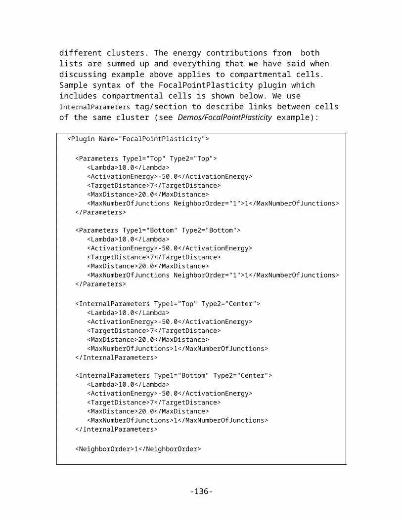
This is how we do it using mathematical formulas:
First we define shift vector as a vector difference between vector pointing to center of mass of the lattice and vector pointing to (approximately) the middle of the lattice.Next we shift cell to the middle of the lattice using :
where denotes center of mass position of a cell after shifting but before adding or subtracting a pixel.Next we take into account the new pixel (either gained or lost) and calculate center of mass position (for the shifted cell):
Above we have assumed that we are adding one pixel.
Now all that we need to do is to shift back by same vector that brought cell to (approximately) center of the lattice.
We are almost done. We still have to check if is inside the lattice. If this is not the case we need to shift it back to the lattice but now we are allowed to use only a vector whose components are multiples of lattice dimensions (and we can safely restrict to +1 and -1 multiples of the lattice dimmensions) . For example we may have:
where , , are dimensions of the lattice.There is no cheating here. In the lattice with periodic boundary conditions you are allowed to shift point coordinates a vector whose components are multiples of lattice dimensions.All we need to do is to examine new center of mass position and form suitable vector .
11.55. Dividing cluster cells
While dividing non-clustered cells is straightforward, doing the same for clustered cells is more challenging. To divide non-cluster cell using directional mitosis algorithm we construct a line or a plane passing through center of mass of a cell and pixels of the cell (we are using PixelTracker plugin with mitosis) on one side of the line/plane end up in child cell and the rest stays in parent cell. The orientation of the line/plane can be either specified by the user or we can use CC3D built-in feature to calculate calculate orientation tion of principal axes and divide either along minor or major axis.
With compartmental cells, things get more complicated because: 1) Compartmental cells are composed of many subcells. 2) There can be different topologies of clusters. Some clusters may look “snake-like” and some might be compactly packed blobs of subcells. The algorithm which we implemented in CC3D works in the following way:
-136-
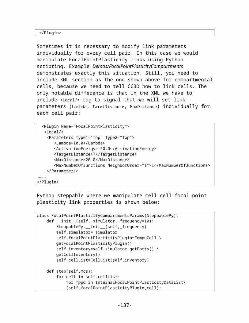
1o2o
1o2o
1) We first construct a set of pixels containing every pixel belonging to a cluster cell. You may think of it as of a single “regular” cell.
2) We store volumes of compartments so that we know how big compartments shold be after mitosis (they will be half of original volume)
3) We calculate center of mass of entire cluster and calculate vector offsets between center of mass of a cluster and center of mass of particulat compartments as on the figure below:
Figure 25. Vectors o1 and o2 show offsets between center of mass of a cluster and center of mass particular compartments.
4) We pick division line/plane and for parents and child cells we offsets between cluster center of mass (after mitosis) and center of masses of clusters. We do it according to the formula:
p= o−12
( o⋅n ) n
where p denotes offset after mitosis from center of mass of child (parent) clusters, o is orientation vector before mitosis (see picture above) and n is a normalized vector perpendicular to division line/plane. If we try to divide the cluster along dashed line as on the picture below
Figure 26. Division of cell along dashed line. Notice the orientation of n
the offsets after the mitosis for child and parent cell will be p1=1
2o1
and p2=o2as expected because both parent and child cells will retain their heights but after mitosis will become twice narrower (cell with grey outer compartments is a parent cell):
-137-

Figure 27. Child and parent (the one with grey outer compartments) cells after mitosis.The formula given above is heuristic. It gives fairly simple way of assigning pixels of child/parent clusters to cellular compartments. It is not perfect but the idea is to get approximate shape of the cell after the mitosis and as simulation runs cell shape will readjust based on constraints such as adhesion of focal point plasticity. Before continuing with the mitosis we check if center of masses of compartments belong to child/parent clusters. If the center of masses are outside their target pixels we abandon mitosis and wait for readjustment of cell shape at which point mitosis algorithm will pass this sanity check. For certain “exotic” shapes of cluster shapes presented mitosis algorithm may not work well or at all . In this case we would have to write specialized mitosis algorithm.5) We divide clusters and knowing offsets from child/parent cluster center of mass
we assign pixels to particular compartments. The assignment is based on the distance of particular pixel to center of masses of clusters. Pixel is assigned to particular compartment if its distance to the center of mass of the compartment is the smallest as compared to distances between centroids of other compartments. If given compartment has reached its target volume and other compartmets are underpopulated we would assign pixels to other compartments based on the closest distance criterion. Altohugh this method may result in some deviation from perfect 50-50 division of compartment volume in most cases after few MCS cells will readjust their volume.
Figure 28. CC3D example of compartmental cell division. See also examples_PythonTutorial/clusterMitosis.
11.67. Command line options of CompuCell3DAlthough most users run CC3D using Player GUI sometimes it is very convenient to run CC3D using command line options. CC3D allows to invoke Player directly from command line which is convenient because if saves several clicks and if you run many simulations this might be quite convenient.
-138-

Remark: On Windows we use .bat extension for run scripts and on Linux/OSX it is .sh. Otherwise all the material in this section applies to all the platforms.
11.6.1 7.1. CompuCell3D Player Command Line Options
The command line options for running simulation with the player are as follows:
compucell3d.bat [options]
Options are:
-i <simulation file> - users specify simulation file they want to run. It can be either CC3DML (XML) configuration file or Python script.
-s <screenshotDescriptionFileName> - name of the file containing description of screenshots to be taken with the simulation. Usually this file is prepared using Player by switching to different views, clickin camera button and saving screenshot description file from the Player File menu.
-o <customScreenshotDirectoryName> - allows users to specify where screenshots will be written. Overrides default settings.
--noOutput - instructs CC3D not to store any screenshots. Overrides Player settings.
--exitWhenDone - instructs CC3D to exit at the end of simulation. Overrides Player settings.
-h, --help - prints command line usage on the screen
Example command may look like:
compucell3d.bat –i Demos\cellsort_2D\cellsort_2D.xml –s screenshotDescription.sdfml –o Demos\cellsort_2D\screenshot
The frequency of the screenshots is read using Player settings so if you need to adjust it please use either GUI directly or change it using PlayerSettings plugin (see example Demos\cellsort_2D\cellsort_2D_PlayerSettings.xml)
11.6.2 7.2. Runnig CompuCell3D in a GUI-Less Mode - Command Line Options.
Sometimes when you want to run CC3D on a cluster you will have to use runScript.bat which allows running CC3D simulations without invoking GUI. However, all the screenshots will be still stored.
-139-

Remark: current version of this script does not handle properly relative paths so it has to be run from the installation directory of CC3D i.e. you have to cd into this directory prior to runnit runScript.bat. Another solution is to use full paths.
The output of this script is in the form of vtk files which can be subsequently replayed in the Player (and one can take screenshots then). By default all fields present in the simulation are stored in the vtk file. If users want to remove some of the fields fro mbeing stored in the vtk format they have to pass this information in the Python script:
CompuCellSetup.doNotOutputField(_fieldName)The best place to put such stetements is directly before steppable section in the Python main script. See also commented line (and try uncommenting it) in examples_PythonTutorial\ diffusion_extra_player_field\ diffusion_2D_extra_player_field.py. Storing entire fields (as opposed to storing screenshots) preserves exact snapshots of the simulation and allows result postprocessing. In addition to the vtk files runScript stores lattice description file with .dml extension which users open in the Player (File->Open Lattice Description Summary File…) if they want to reply generated vtk files.
The format of the command is:
runScript.bat [options]
The command line options for runScript.bat are as follows:
-i <simulation file> - users specify simulation file they want to run. It can be either CC3DML (XML) configuration file or Python script. Remember about using full paths if you run the script from directory different than -c <outputFileCoreName> - allows users to specify core name for the vtk files. The default name for vtk files is “Step”
-o <customVtkDirectoryName> - allows users to specify where vtk files and the .dml file will be written. Overrides default settings
-f <frequency> or –outputFrequency=<frequency> - allows to specify how often vtk files are stored to the disk. Those files tend to be quite large for bigger simulations so storing them every single MCS (default setting) slows down simulation considerably and also uses a lot of disk space.
--noOutput - instructs CC3D not to store any output. This option makes little sense in most cases.
-h, --help - prints command line usage on the screen
Example command may look as follows:
-140-
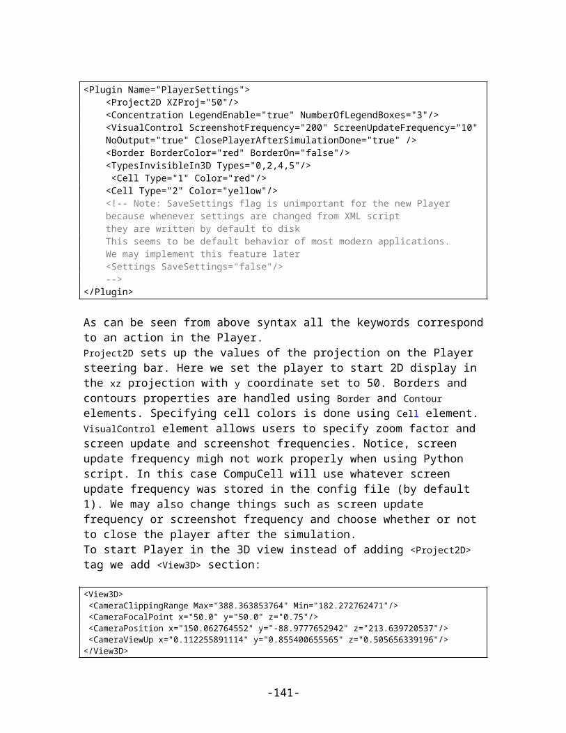
runScript.bat –i examples_PythonTutorial\cellsort_2D_info_printer\ cellsort_2D_info_printer.py –f 10 –o examples_PythonTutorial\cellsort_2D_info_printer\screenshots–c infoPrinter
11.78. Managing CompuCell3D simulations (CC3D project files)Until version 3.6.0 CompuCell3D simulations were stored as a combination of Python, XML, and PIF files. This solution was working fine but there were significant problems with keeping track of simulations files. We still support this convention. However, starting with version 3.6.0 we introduced new way of managing CC3D simulations by enforcing that a single CC3D simulation is stored in a folder containing .cc3d project file describing simulation resources (.cc3d is in fact XML), such as XML configuration file, Python scripts, PIF files, Concentration filets etc… and a directory called Simulation where all the resources reside. The structure of the new-style CC3D simulation is presented in the diagram below:
->CellsortDemoCellsortDemo.cc3d
->SimulationCellsort.xmlCellsort.pyCellsortSteppables.pyCellsort.piffFGF.txt
Bold fonts denote folders. The benefit of using CC3D project files instead of loosely related files are as follows:
1) Previously users had to guess which file needs to be open in CC3D – XML or Python. While in a well written simulation one can link the files together in a way that when user opens either one the simulation would work but, nevertheless, such approach was clumsy and unreliable. Starting with 3.6.0 users open .cc3d file and they don’t have to stress out that CompUCell3D will complain with error message.
2) All the files specified in the .cc3d project files are copied to the result output directory along with simulation results (uncles you explicitely specify otherwise). Thus, when you run multiple simulations each one with different parameters, the copies of all XML and Python files are stored eliminating guessing which parameters were associated with particular simulations.
3) All file paths appearing in the simulation files are relative paths with respect to main simulation folder. This makes simulations portable because all simulation resources are contained withing single folder. In the example above when referring to Cellsort.piff file from Cellsort.xml you use “Simulation/ Cellsort.piff”. This effectively eliminates drawbacks of previous approach – when user one stores his simulations in Demos/cellsort and gives this simulation to his colleague who stores simulation in MySimulations/cellsort then second user will most likely see error message informing him that file
-141-

“Demos/cellsort/cellsort.piff” was not found (I assume here that initial condition is specified using cellsort.piff). With approach based on relative paths such problems do not exist. Second user can put the simulation anywhere he wants and it will run just fine.
4) New style of storing CC3D simulations has also another advantage – it makes graphical management of simulation content and simulation generation very easy. As amatetr of fact new component of CC3D suite – Twedit++ - CC3D edition has a graphical tool that allows for easy project file management and it also has new simulation wizadrd which allows users to build template of CC3D simulation within less than a minute.
Let’s now look in detail at the structure of .cc3d files:
<Simulation version="3.6.0"> <XMLScript>Simulation/Cellsort.xml</XMLScript> <PythonScript>Simulation/Cellsort.py</PythonScript> <Resource Type="Python">Simulation/CellsortSteppables.py</Resource> <PIFFile>Simulation/Cellsort.piff</PIFFile> <Resource Type="Field" Copy="No">Simulation/FGF.txt</Resource></Simulation>
As you can see the structure of the file is quite flat. All that we are storing there is names of files that are used in the simulation. Two files have special tags <XMLFile> which specifies name of the XML file storing “XML portion” of the simulation and <PythonScript> which specifies main Python script. We have also PIFFile tag which is used to designate PIF files. All other files used in the simulation are referred to as Resources. For example Python steppable file is a resource of type “Python”. FGF.txt is aresource of type “Field”. Notice that all the files are specified using paths relative to main simulation directory.As we mentioned before, when you run .cc3d simulation all the files listed in the project file are copied to result folder. If for somereason oyu want to avoid coping of some of the files, simply add Copy=”No” attribute in the tag with file name specification.
11.89. Keeping Track of Simulation Files (deprecated)CompuCell3D will store screenshots, vtk lattice snapshots and CC3DML file/Python main script in the output directory. However often simulations consist of several files: CC3DML, Python main script, Python steppable script, Python plugin script, PIF files etc. If you want those files to be archived with the rest of simulation output you need to use SimulationFileStorage steppable declared in PySteppablesExamples.py.
The usage is very simple (see also examples_PythonTutorial\cellsort_2D_info_printer\cellsort_2D_info_printer.py):
from PySteppablesExamples import SimulationFileStoragesfs=SimulationFileStorage(_simulator=sim,_frequency=10)
-142-

sfs.addFileNameToStore("\examples_PythonTutorial/cellsort_2D_info_printer/cellsort_2D.xml")sfs.addFileNameToStore("\examples_PythonTutorial/cellsort_2D_info_printer/cellsort_2D_info_printer.py")sfs.addFileNameToStore("examples_PythonTutorial/cellsort_2D_info_printer\/cellsort_2D_steppables_info_printer.py")steppableRegistry.registerSteppable(sfs)
It wil ensure that files listed here will be writte to simulation directory. This way if you keep changing simulation files you will be able to easily recover entire simulation at
-143-