INTRODUÇÃO À GEOESTATÍSTICA 7-Introduction to Stochastic ... · Geostatistical Models:...
37
7-Introduction to Stochastic Simulation INTRODUÇÃO À GEOESTATÍSTICA Amílcar Soares CERENA-IST [email protected]
Transcript of INTRODUÇÃO À GEOESTATÍSTICA 7-Introduction to Stochastic ... · Geostatistical Models:...

7-Introduction to Stochastic
Simulation
INTRODUÇÃO À
GEOESTATÍSTICA
Amílcar Soares
CERENA-IST
Objective of Geostatistical
Simulation Models : Integration of the
concept of uncertainty in high resolution
static models of the oil reservoirs.
Applications: simulation of lithofacies,
simulation of petrophysical properties,
seismic inversion, geostatistical history
matching.
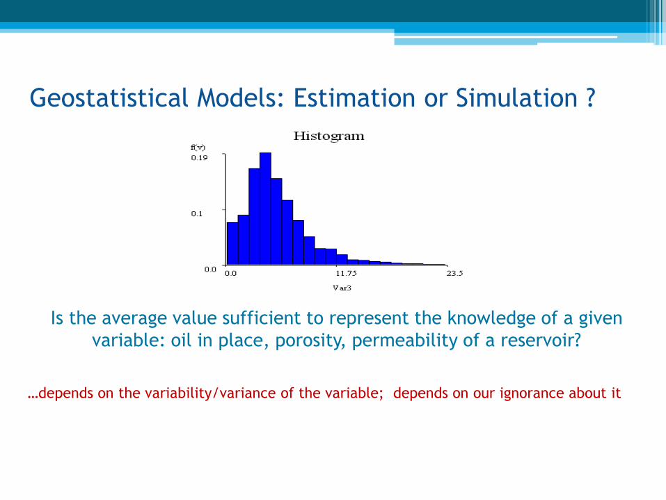
Geostatistical Models: Estimation or Simulation ?
Is the average value sufficient to represent the knowledge of a given
variable: oil in place, porosity, permeability of a reservoir?
…depends on the variability/variance of the variable; depends on our ignorance about it
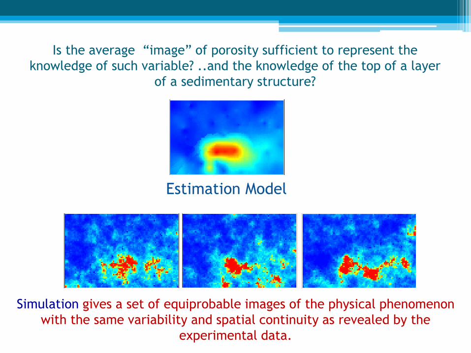
Is the average “image” of porosity sufficient to represent the
knowledge of such variable? ..and the knowledge of the top of a layer
of a sedimentary structure?
Estimation Model
Simulation gives a set of equiprobable images of the physical phenomenon
with the same variability and spatial continuity as revealed by the
experimental data.
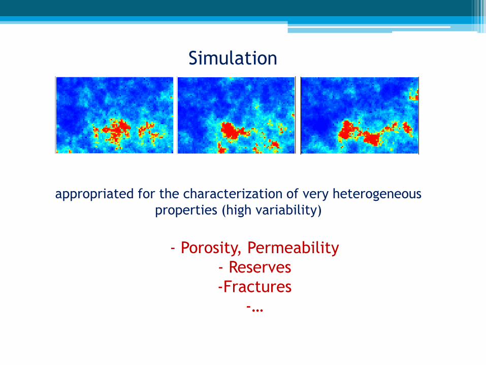
Simulation
appropriated for the characterization of very heterogeneous
properties (high variability)
- Porosity, Permeability
- Reserves
-Fractures
-…

Stochastic Simulation of Heterogeneous Variables
Main purpose: Integration of the uncertainty in the oil reservoir models
for decision making processes

The Concept of Uncertainty
Porosity,
permeability,..
Response of the dynamic
model of reserves
Estimated model of the most
probable values
Provides only the dynamic response of the most likely model which is not
necessarily the most likely response
It provides no measure of uncertainty, extreme values , risk, etc...
Only one response: pressure
curves, water cut, ..

...
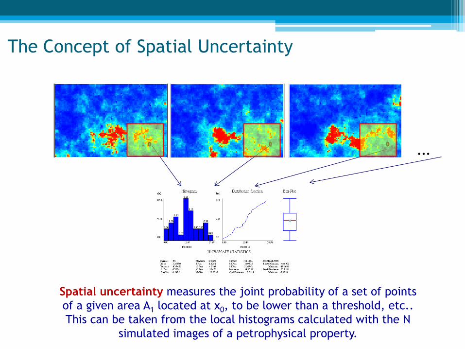
The Concept of Spatial Uncertainty
For any spatial location x0, uncertainty measures can be taken from the local
histograms calculated with the N simulated images of a petrophysical property,
...
The Concept of Spatial Uncertainty
Spatial uncertainty measures the joint probability of a set of points
of a given area A1 located at x0, to be lower than a threshold, etc..
This can be taken from the local histograms calculated with the N
simulated images of a petrophysical property.

The Concept of Uncertainty
Porosity,
permeability,..
Response of the dynamic
model of reserves
Quantifying the uncertainty of internal properties in terms of reserves,
risk analysis, ...Uncertainty is measured in the responses of a dynamic
simulator (non-linear function of petrophysical properties).
Simulated Model
Uncertainty of Reserves
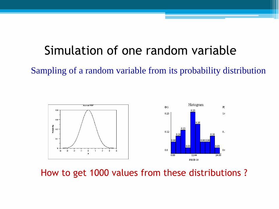
Simulation of one random variable
Sampling of a random variable from its probability distribution
How to get 1000 values from these distributions ?
The Monte Carlo method
“the use of random numbers to solve deterministic systems or stochastic
models”
1- Inverse transform sampling
2- Acceptance / Rejection method
(Rejection Sampling)
Simulation of one random variable
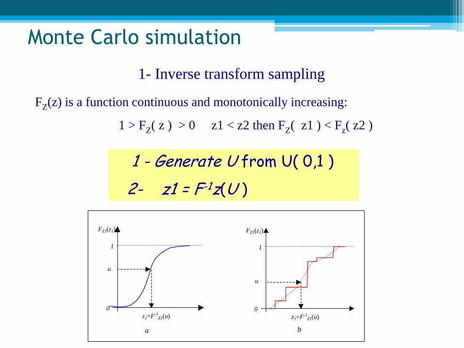
FZ(z) is a function continuous and monotonically increasing:
1 > FZ( z ) > 0 z1 < z2 then FZ( z1 ) < Fz( z2 )
1 - Generate U from U( 0,1 )
2- z1 = F-1z(U )
0
1
FZ1(z1)
u
z1=F-1Z1(u)
0
1
FZ1(z1)
u
z1=F-1Z1(u)
a b
1- Inverse transform sampling
Monte Carlo simulation

Monte Carlo simulation
2- Acceptance / Rejection method
(Rejection Sampling)
Specify a function (x) that upper bounds the density function f: t(x) >= f(x) for all x.
1
xdxfxdxtc
x1 is accepted
x2 is accepted
x1 is rejected
x2 is rejected
x1 x2
f(x)
t(x)
r(x) = t(x) / c is a density function
1- Generate x
2- Generate u from U( 0,1 )
3- u <= f(x) / t(x) x is accepted
Otherwise x is rejected

Algorithms to generate continuous random variables
Uniform
Inverse method: Generate U U( 0,1 ) Returns X = F-1( U )
1 - Generates U U( 0,1 )
2 - Returns X = a + ( b - a ) . U
Exponential
1 - Generates U U( 0,1 )
2 - Returns X = - . ln(U)
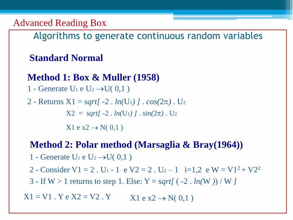
Algorithms to generate continuous random variables
Standard Normal
1 - Generate U1 e U2 U( 0,1 )
2 - Returns X1 = sqrt[ -2 . ln(U1) ] . cos(2) . U2
Method 1: Box & Muller (1958)
X2 = sqrt[ -2 . ln(U1) ] . sin(2) . U2
X1 e x2 N( 0,1 )
Method 2: Polar method (Marsaglia & Bray(1964))
1 - Generate U1 e U2 U( 0,1 )
2 - Consider V1 = 2 . U1 - 1 e V2 = 2 . U2 – 1 i=1,2 e W = V12 + V22
3 - If W > 1 returns to step 1. Else: Y = sqrt[ ( -2 . ln(W )) / W ]
X1 = V1 . Y e X2 = V2 . Y X1 e x2 N( 0,1 )
Advanced Reading Box

Algorithms to generate continuous random variables
Lognormal
1 – Generate Y N ( ,2 )
2 – Returns X = eY
Triangular
Note that X triang( 0, 1, ( c – a ) / ( b – a ) ), so X‘ = a + ( b - a )X triang( a, b, c )
1 – Generate U U ( 0,1 )
2 – If U c returns X = sqrt( c . U );
Else: returns X = 1 - sqrt[ ( 1 - c) ( 1 – U ) ]
Advanced Reading Box

Simulation of empirical distributions
Sort decreasingly the n values of Z;
Calculate pi=(i-0.5)/n associated to the sorted Zi
1 – Generate U U (0,1)
2 – Returns the value Z = Zi + ( Zi+1 – zi ) . ( pi – U ) / ( pi - pi+1 )
Ex: n=100 values: 2.1, 0.3, 11.4, ….. After sorting, to each value Zi is associated the following “cumulative probability” pi:
min=Z1=0.3 p1=0.005; Z2=0.6 p2=0.015; Z3=0.65 p3=0.025;…;
max=Z100=11.4 p100=.995
Consider U=0.1 returns Z=0.3+.5x(0.6-0.3)=0.45
Create a cumulative “probability of Z”;
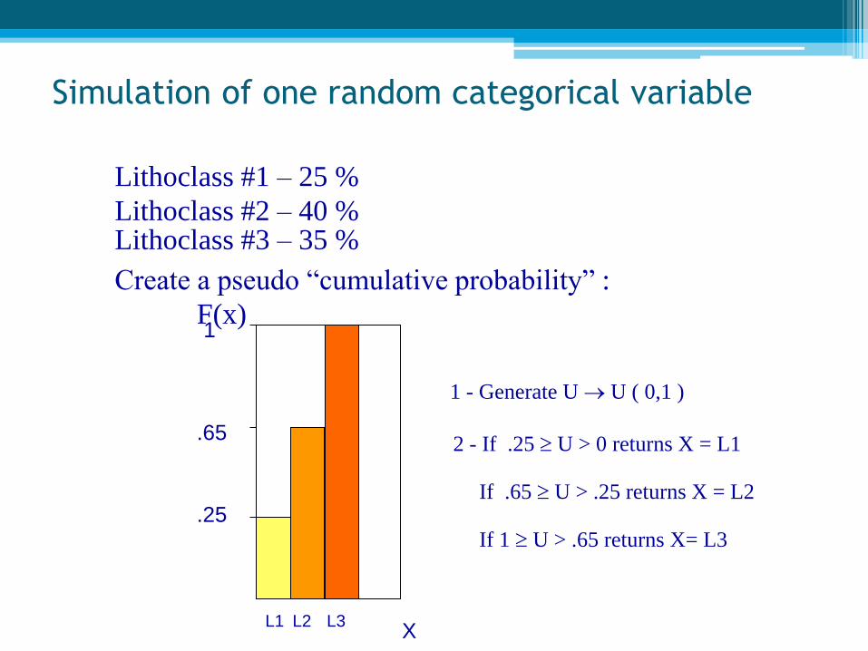
Simulation of one random categorical variable
Lithoclass #1 – 25 %
Lithoclass #2 – 40 % Lithoclass #3 – 35 %
Create a pseudo “cumulative probability” :
.25
.65
1
L1 L2 L3
1 - Generate U U ( 0,1 )
2 - If .25 U > 0 returns X = L1
If .65 U > .25 returns X = L2
If 1 U > .65 returns X= L3
F(x)
X
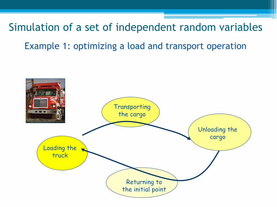
Simulation of a set of independent random variables
Example 1: optimizing a load and transport operation
Loading the truck
Unloading the cargo
Transporting the cargo
Returning to the initial point
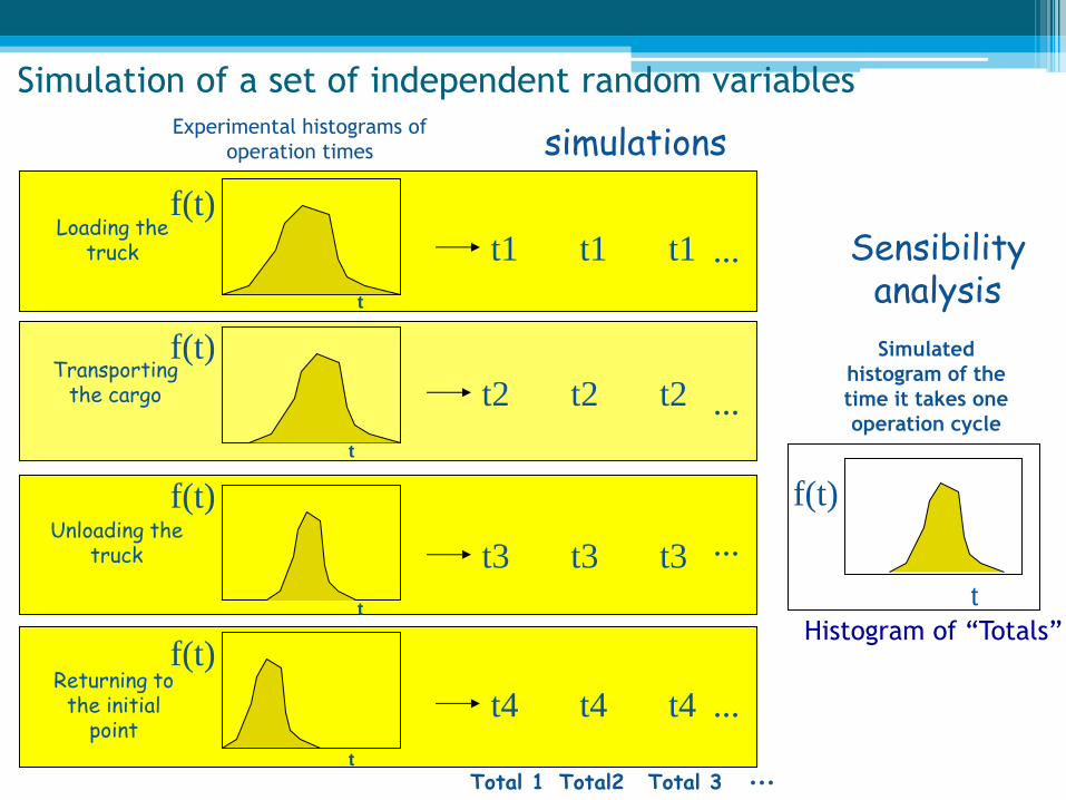
Experimental histograms of
operation times simulations
Total 1 Total2
Unloading the truck
t
f(t)
t3 t3 t3
Total 3
t
f(t)
Simulated
histogram of the
time it takes one
operation cycle
...
Returning to the initial
point t
f(t)
t4 t4 t4 ...
...
Transporting the cargo
t
f(t)
t2 t2 t2 ...
Loading the truck
t
f(t)
t1 t1 t1 ... Sensibility analysis
Simulation of a set of independent random variables
Histogram of “Totals”
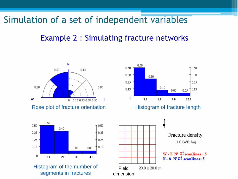
Rose plot of fracture orientation
Histogram of the number of
segments in fractures
Example 2 : Simulating fracture networks
Fracture density
Field
dimension
Histogram of fracture length
of of
Simulation of a set of independent variables

1st simulation Superimposing of a 2ª simulation over a
different set of fractures
Simulation of 355 fractures Simulation of 513 fractures
Simulation of a set of independent variables
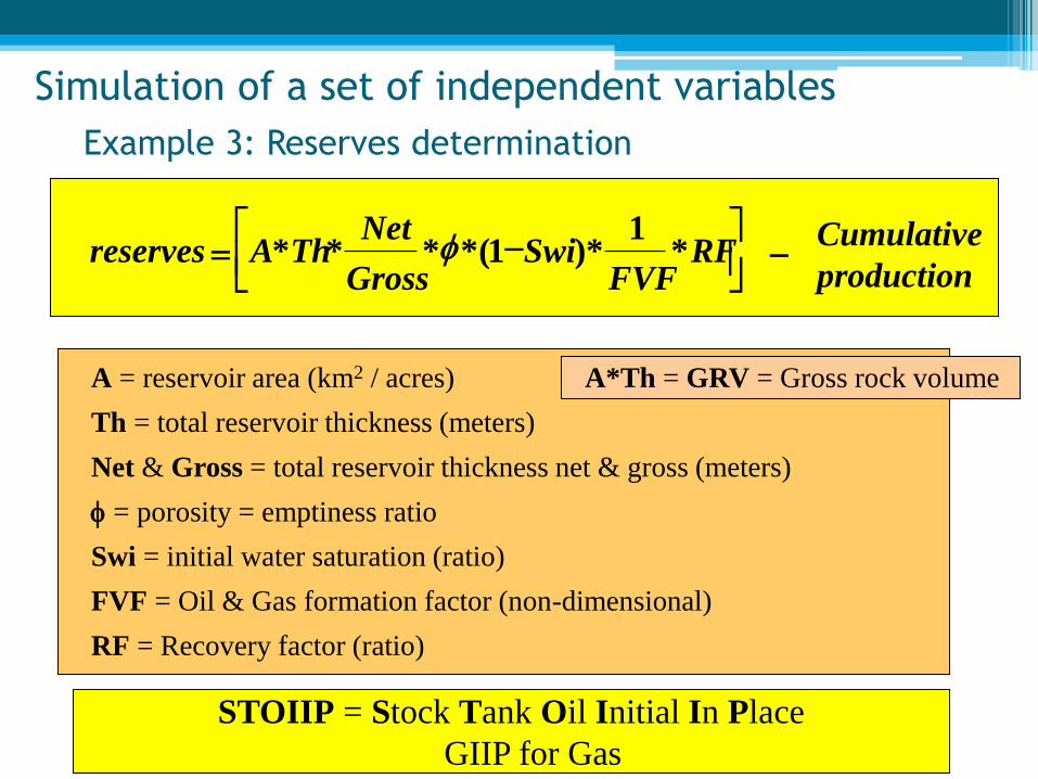
Example 3: Reserves determination
reserves A Th Net
Gross Swi
FVF RF
Cumulative
production
* * * * ( ) * * f 1
1
STOIIP = Stock Tank Oil Initial In Place
GIIP for Gas
A = reservoir area (km2 / acres)
Th = total reservoir thickness (meters)
Net & Gross = total reservoir thickness net & gross (meters)
f = porosity = emptiness ratio
Swi = initial water saturation (ratio)
FVF = Oil & Gas formation factor (non-dimensional)
RF = Recovery factor (ratio)
A*Th = GRV = Gross rock volume
Simulation of a set of independent variables

PDFs of input variables:

Simulation of two dependent random variables
When two random variables show some statistical dependence, one
whish to generate both by reproducing the marginal distributions F(Z1 )
and F(Z2 ) but also the joint distribution of probabilities F( Z1, Z2 )
To reproduce the joint distribution K and Φ
(high values of K correspond to high values
of Φ ) they can not be simulated
independently
..let us suppose that one whish to simulate pairs of porosity e permeability
values that show a positive correlation

Principle of Sequential Simulation
Applying Bayes law in sequential steps: F( Z1, Z2 ) = F( Z2 | Z1 ) . F(Z1)
Simulating two values z1 e z2 from a joint distribution
F( Z1,Z2 ):
1st Generate z1 from pdf F(Z1).
2nd Generate z2 from conditional distribution function F( Z2 | Z1=z1)
Simulation of two dependent random variables

Monte Carlo simulation
Simulating two variables from bivariate distribution:
Permeability and porosity
K
f
z1 Fz1
K z1
u
F(f|K=z1)
f z2
u
1- simulate the first
value of K from the
marginal distribution
of permeability by
using a Monte Carlo
algorithm
2- From the joint
distributtion F(Φ,K),
extract the conditional
distribution: F(Φ|K=z1)
3- Simulate the porosity
value Φ =z2 from the
conditional distribution:
F(Φ|K=z1), by using a Monte
Carlo algorithm
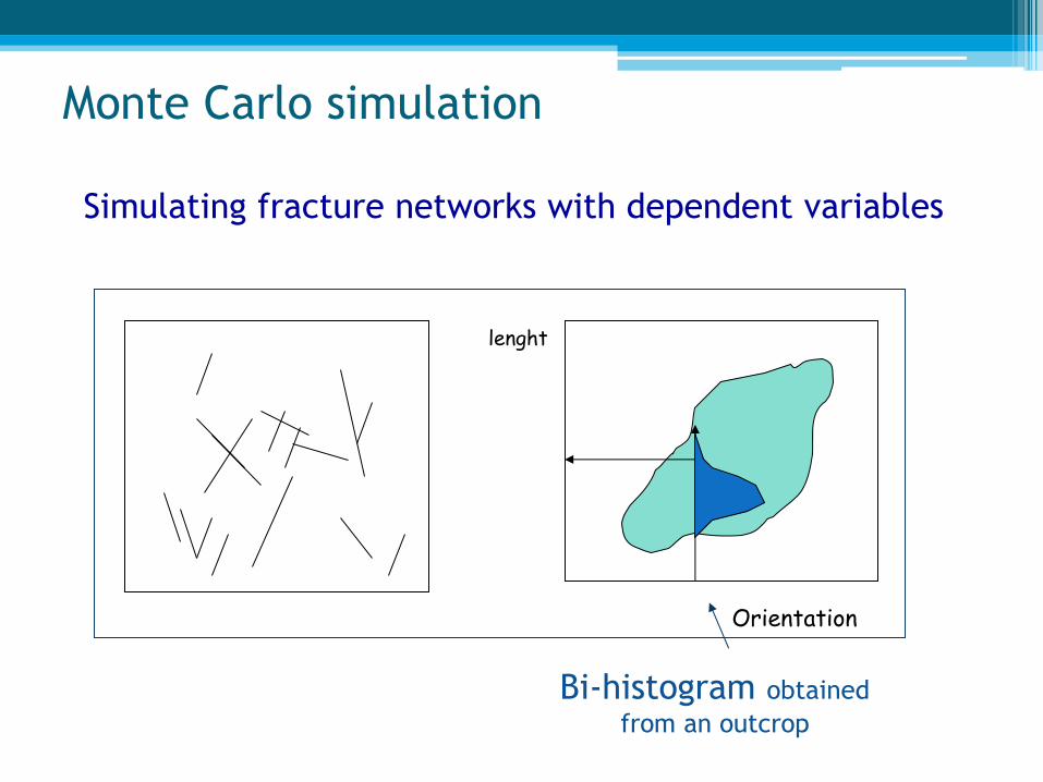
Monte Carlo simulation
Simulating fracture networks with dependent variables
Orientation
lenght
Bi-histogram obtained
from an outcrop

F(Z1,Z2,….,ZN)=F(Z1).F(Z2|Z1).F(Z3|Z1,Z2,Z3)… F(ZN|Z1,…ZN-1)
Generate (simulate) a set of values z1,…,zN from the
distribution law F(Z1,Z2,…,ZN), which can be made from
sequential steps:
1º- We generate a value z1 from the marginal law F(Z1)
2º- Than we simulate a value z2 from the conditional
distribution law F(Z2|Z1=z1)
Simulate value zN from F (ZN |Z1=z1,Z2=z2,…,ZN-1=zN-1)
Simulating N random dependant variables

Example: Simulation of values Zi on a regular grid using 5 known samples
Sequential simulation of spatial phenomena

Sequential simulation of spatial phenomena
OBJECTIVE: simulation values from F(Z6,Z7,Z8,….,Z64 | Z1, Z2,Z3,Z4,Z5)
1- Simulating one value z6 from
F(Z6 | Z1, Z2,Z3,Z4,Z5)
2- Simulating a value z7 from
F(Z7 | Z1, Z2,Z3,Z4,Z5,Z6)
F(Z7 | Z1, Z2,Z3,Z4,Z5,Z6)
F(Z6 | Z1, Z2,Z3,Z4,Z5)
F(Z8 | Z1, Z2,Z3,Z4,Z5,Z6,Z7)
3- Simulating a value z8 from
F(Z8 | Z1, Z2,Z3,Z4,Z5,Z6,Z7)
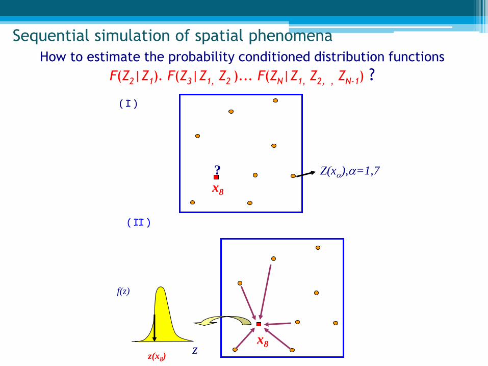
Sequential simulation of spatial phenomena
Z(x),=1,7 ?
x8
z
f(z)
z(x8)
x8
( II )
( I )
How to estimate the probability conditioned distribution functions
F(Z2|Z1). F(Z3|Z1, Z2 )... F(ZN|Z1, Z2, , ZN-1) ?

x8
Z(x),=1,8
?
x8
z
f(z)
z(x9)
x9
( IV)
( III )
x8

Example : Sequential simulation of 3 lithofacies: t1, t2 andt3
?
Prob x0 t1 =60%
Prob x0 t2=25%
Prob x0 t3 =15%
1-
60%
85%
100%
2-
1- Random choice of one node on the regular grid,
x0 .
2- Estimate the local probabilities
3- Create the Pseudo local cumulative
law of distribution:

If r<.6 then x0 t1
If r>=.6 and r<..85 then x0 t2
If r>=.85 then x0 t3
Monte Carlo: Generating r from U(0,1)
60%
85%
100%
3- Simulating T1, T2 e T3 in x0: 3-
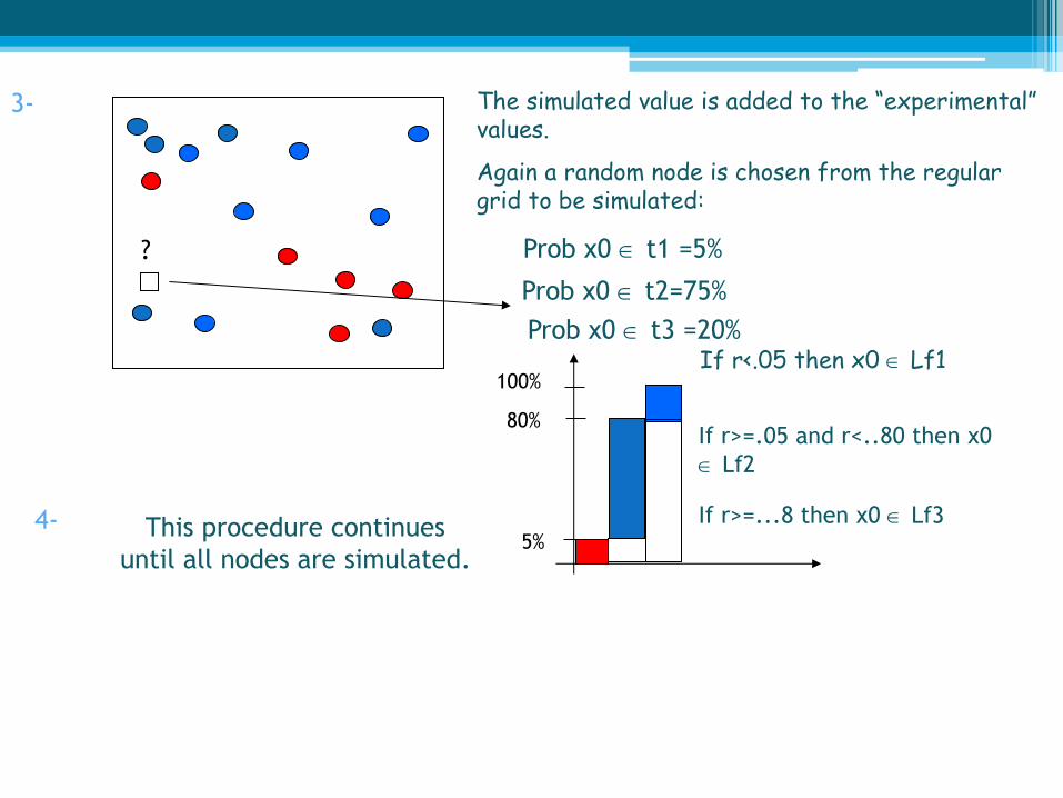
3- The simulated value is added to the “experimental” values.
Again a random node is chosen from the regular grid to be simulated:
? Prob x0 t1 =5%
Prob x0 t2=75%
Prob x0 t3 =20%
5%
80%
100% If r<.05 then x0 Lf1
If r>=.05 and r<..80 then x0
Lf2
If r>=...8 then x0 Lf3
4- This procedure continues
until all nodes are simulated.