Intro to the DRFM. - ITS · ISART: Radar Fundamentals – Slide 2 ©2011 Greg Showman Rules of...
68
ISART: Radar Fundamentals – Slide 1 ©2011 Greg Showman Radar Fundamentals A Tutorial Presented to the 12th Annual International Symposium on Advanced Radio Technologies (ISART) July 27, 2011 Dr. Gregory A. Showman 404-407-7719 [email protected]
-
Upload
nguyendang -
Category
Documents
-
view
221 -
download
3
Transcript of Intro to the DRFM. - ITS · ISART: Radar Fundamentals – Slide 2 ©2011 Greg Showman Rules of...

ISART: Radar Fundamentals – Slide 1
©2011 Greg Showman
Radar Fundamentals
A Tutorial Presented to the
12th Annual International Symposium on
Advanced Radio Technologies (ISART)
July 27, 2011
Dr. Gregory A. Showman
404-407-7719

ISART: Radar Fundamentals – Slide 2
©2011 Greg Showman
Rules of Engagement
This tutorial is “radar according to Greg”
Based on my experiences and understanding
Tailored to ISART-11
This tutorial is not exhaustive
There are always exceptions
Shooting for the “90th-percentile”

ISART: Radar Fundamentals – Slide 3
©2011 Greg Showman
Outline
Background and Range Measurement
SNR and the Matched Filter
Radar Range Equation
Detection in Noise
Pulse Compression
Multiple Pulses
Antenna Effects

ISART: Radar Fundamentals – Slide 4
©2011 Greg Showman
Radar Applications and Functions
Point Targets
Detection
Estimation
Tracking
Targets: Cars (police radar), aircraft (air traffic control), reentry vehicles (ballistic missile early warning)
Continuum Targets
Real-Beam Imaging
Synthetic Aperture Imaging
“Targets”: 1-D target (range profile), 2-D clutter (terrain) and 3-D clutter (weather)"
Air Defense
Airborne interceptor
Air-to-Ground Surveillance
Anti-Air Warfare

ISART: Radar Fundamentals – Slide 5
©2011 Greg Showman
Electromagnetic (EM) Spectrum
1 km
1 m
1 mm
1
1Å
0.3
300
3 x 10⁵
f (MHz)
Radio Telegraphy
Broadcast
Short Wave
Conventional Radar
Millimeter Radar
Infrared
Visible
Ultra Violet
X-Rays
Gamma Rays
HF = 3 - 30 MHz
VHF = 30 - 300 MHz
UHF = 300 - 1000 MHz
L-Band = 1 - 2 GHz
S-Band = 2 - 4 GHz
C-Band = 4 - 8 GHz
X-Band = 8 - 12 GHz
Ku-Band = 12 - 18 GHz
Ka-Band = 27 - 40 GHz
W-Band = 75 - 110 GHz Seekers
Fire Control (Trackers)
Search
Long Range
Short Range
Radar Applications / Bands
f=c
f=frequency (cycles per second)
=wavelength (m)
c= speed of light (3x10⁸m/s)
3
30

ISART: Radar Fundamentals – Slide 6
©2011 Greg Showman
Continuous Wave (CW) vs. Pulsed
Continuous Wave (CW) operation properties
Simultaneous TX and RX
Simple TX and RX hardware
Good Doppler measurements
BUT, operation is limited to
Low power short ranges
Or bistatic complicated implementation
Pulsed operation properties
Time multiplexing of high-power TX and sensitive RX
Sharing of TX and RX apertures
Good range measurements

ISART: Radar Fundamentals – Slide 7
©2011 Greg Showman
Waveform Hierarchy
Radar Waveforms
CW Radars Pulsed Radars
Frequency
Modulated CW
Phase
Modulated CW:
bi-phase & poly-phase
Linear FMCW,
Sawtooth, or
Triangle
Nonlinear FMCW,
Sinusoidal,
Multiple Frequency,
Noise, & Pseudorandom
Intra-pulse Modulation
Pulse to Pulse Modulation:
Frequency Agility
Stepped Frequency
Frequency Modulated:
Linear FM
Nonlinear FM
Phase Modulated:
Bi-phase
Poly-phase
Low Power
or
Bistatic
High Power
and
Monostatic

ISART: Radar Fundamentals – Slide 8
©2011 Greg Showman
Radar Environment
Clutter
Radar
Target
EMI
EA
•Transmits: Electromagnetic wave
•Receives:
•Echoes from targets, clutter
•Electromagnetic interference (EMI)
•Electronic attack (EA)
•External environmental noise
•Internal system noise
•Measures (varies with radar):
•Azimuth, Elevation
•Range
•Doppler shift
•Amplitude
•Polarization

ISART: Radar Fundamentals – Slide 9
©2011 Greg Showman
Radio Detection and Ranging R
radar
target
c TD = 2 R
TD=Time delay between
transmission and
reception of echo
Tp = PRI
TD
R = c TD / 2
Round-trip
path length:
Range:
TD = 1 s R = 150 m
TD = 10 s R = 1.5 km
TD = 100 s R = 15 km
TD = 1 ms R = 150 km

ISART: Radar Fundamentals – Slide 10
©2011 Greg Showman
Outline
Background and Range Measurement
SNR and the Matched Filter
Radar Range Equation
Detection in Noise
Pulse Compression
Multiple Pulses
Antenna Effects

ISART: Radar Fundamentals – Slide 11
©2011 Greg Showman
Signal-To-Noise Ratio
Receiver thermal noise is always present and limits radar performance
Target detection and measurement accuracy are a functions of target signal-to-noise ratio (SNR)
Desire is to maximize SNR
time
Rec
eived
Volt
age
tP1
1 SNRD FAP P
Probability of detection of a
target given a desired
probability of false alarm
SNR
General measurement
standard deviation
ISART: Radar Fundamentals – Slide 12
©2011 Greg Showman
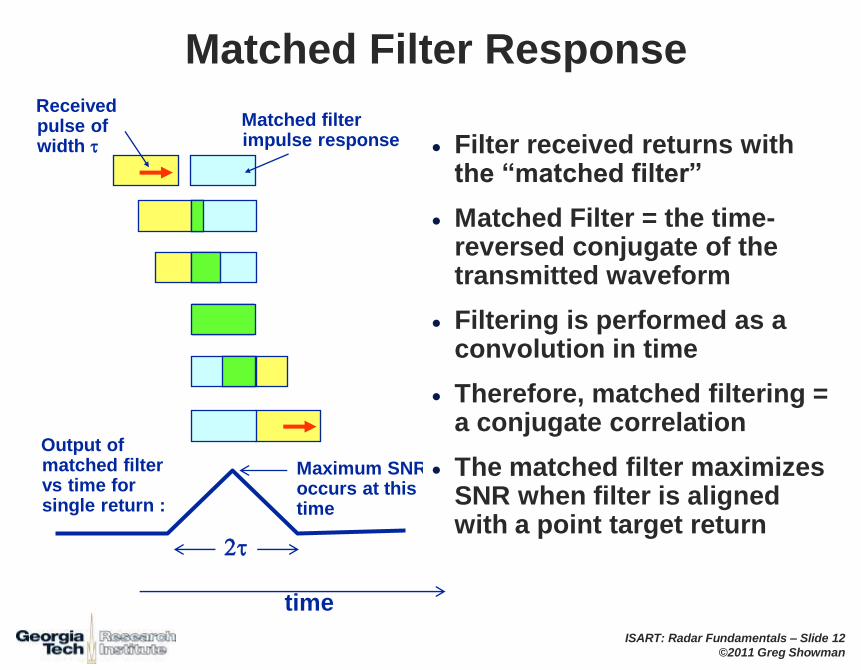
Matched Filter Response
time
Matched filter impulse response
Received pulse of width
Output of matched filter vs time for single return :
2
Maximum SNR occurs at this time
Filter received returns with the “matched filter”
Matched Filter = the time-reversed conjugate of the transmitted waveform
Filtering is performed as a convolution in time
Therefore, matched filtering = a conjugate correlation
The matched filter maximizes SNR when filter is aligned with a point target return

ISART: Radar Fundamentals – Slide 13
©2011 Greg Showman
Outline
Background and Range Measurement
SNR and the Matched Filter
Radar Range Equation
Detection in Noise
Pulse Compression
Multiple Pulses
Antenna Effects

ISART: Radar Fundamentals – Slide 14
©2011 Greg Showman
RADAR RANGE EQUATION (RRE):
Power Density at Range R for Isotropic Radiation
R
(Watts/m2)
Pt
2
1D
4isotropic tP
R
Area of sphere = 4R2
Pt = Radiated power (Watts)

ISART: Radar Fundamentals – Slide 15
©2011 Greg Showman
RADAR RANGE EQUATION :
Power Density at Range R for Main Beam of Directive Antenna
R
Pt
G
Pt G = Effective radiated power (ERP) (Watts)
2
1D
4mainbeam tPG
R
(Watts/m2)
(For a beamwidth of q, most of the power is concentrated
in a solid angle of q2. For an isotropic antenna, the power
is spread over a solid angle of 4. The directive antenna
therefore provides a gain of approximately G=4/q2. For
example, if q=3o 0.0524 radians, G=4,584 36.6 dBi.)

ISART: Radar Fundamentals – Slide 16
©2011 Greg Showman
RADAR RANGE EQUATION : Power Captured by Target
(Watts)
2
1
4r tP PG
R
R
Pt
G
Radiated power
ERP
Power density at target
Power reflected by target
• Radar Cross Section (RCS) is in units of area
• RCS is like a “capture area,” converting flux
(power density) to power
• This captured power is assumed to be uniformly
scattered over 4 steradians
22
24lim
r
Rt
ER
E

ISART: Radar Fundamentals – Slide 17
©2011 Greg Showman
Representative RCS Values
Mean Radar Cross Section of Typical Targets at 1.3-10 GHz
Aircraft (Nose and Tail Aspect)
Small General Aviation 0.6 - 3 m2
Small Fighters 1.5 - 4 m2
Medium Fighters (F-4, et cetera) 4.0 - 10 m2
Small Commercial (DC-9) 10 - 20 m2
Medium Commercial (707, DC-8) 20 - 40 m2
Large Commercial (DC-10, 747) 40 - 100 m2
Ships (5-10 GHz; Approximate Frequency Dependence = f1/2)
Sailboats -- Small 0.5 - 5 plus mast
Military Power Boats 20 - 500 m2
Frigates (1-2 ktons) 0.5 - 1.0 x 10⁴ m2
Destroyers (3-5 ktons) 3.0 - 6.0 x 10⁴ m2
Cruisers (7-20 ktons) 10 - 40 x 104 m2
Carriers (20-40 ktons) 30 - 100 x 104 m2
Tanks 20 - 200 m2
Personnel 0.3 - 1.2 m2
Birds
Sparrow and Starling 0.0003 - 0.001 m2
Pigeon (25-40 knots) 0.001 - 0.01 m2
Mallard (25-40 knots) 0.01 m2
Insects
Moths 0.0001 to 0.000001 m2 (-40 to -70 dBsm)

ISART: Radar Fundamentals – Slide 18
©2011 Greg Showman
RADAR RANGE EQUATION : Received Power Density at Radar Antenna
(Watts)
2 2
1 1
4 4r tP PG
R R
R
Pt
G
Radiated power
ERP
Power density at target
Power reflected by target
Power density at radar

ISART: Radar Fundamentals – Slide 19
©2011 Greg Showman
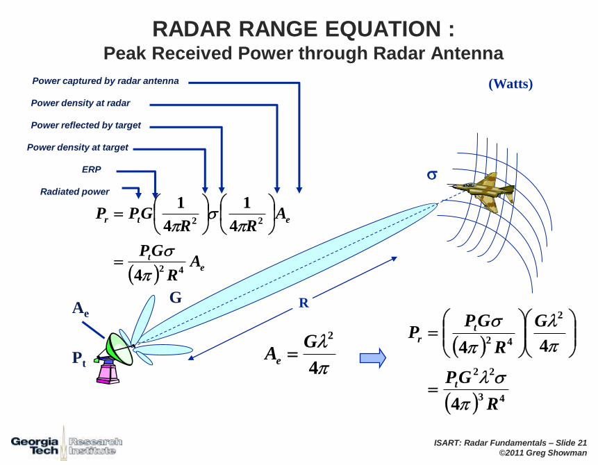
RADAR RANGE EQUATION : Peak Received Power through Radar Antenna
(Watts)
2 2
1 1
4 4r t eP PG A
R R
R
Pt
G Ae
Radiated power
ERP
Power density at target
Power reflected by target
Power density at radar
Power captured by radar antenna

ISART: Radar Fundamentals – Slide 20
©2011 Greg Showman
RADAR RANGE EQUATION : Peak Received Power through Radar Antenna
(Watts)
et
etr
AR
GP
ARR
GPP
42
22
4
4
1
4
1
R
Pt
G Ae
Radiated power
ERP
Power density at target
Power reflected by target
Power density at radar
Power captured by radar antenna
ISART: Radar Fundamentals – Slide 21
©2011 Greg Showman
RADAR RANGE EQUATION : Peak Received Power through Radar Antenna
(Watts)
et
etr
AR
GP
ARR
GPP
42
22
4
4
1
4
1
4
2GAe
43
22
2
42
4
44
R
GP
G
R
GPP
t
tr
R
Pt
G Ae
Radiated power
ERP
Power density at target
Power reflected by target
Power density at radar
Power captured by radar antenna

ISART: Radar Fundamentals – Slide 22
©2011 Greg Showman
Receiver Noise
The target signal competes with receiver
thermal noise:
Thermal noise power = kT0BF
k = 1.38 x 10⁻²³ J/oK (Boltzman’s constant)
T0 = 290 oK
F = receiver noise factor (noise figure)
TS = system noise temperature = T0F
B = receiver bandwidth (Hz)
BandwidthkTB
(dBm)
1 Hz -174
10 Hz -164
100 Hz -154
1 kHz -144
10 kHz -134
100 kHz -124
1 MHz -114
10 MHz -104
100 MHz -94
1 GHz -84
•This is an average power level
•Noise power randomly fluctuates above and below
this level according to its statistical properties

ISART: Radar Fundamentals – Slide 23
©2011 Greg Showman
RADAR RANGE EQUATION: Single Pulse Signal-to-Noise Power Ratio
System
losses
2 2
3 4
04
t
s
PGS
N R L kT BF
Note the dependence on “R-to-the-4th”
Doubling range decreases SNR 12 dB
100 km to 10 km is a 40 dB increase in SNR

ISART: Radar Fundamentals – Slide 24
©2011 Greg Showman
Bandwidth and Pulsewidth
The bandwidth of an unmodulated narrow pulse is approximately B=1/

ISART: Radar Fundamentals – Slide 25
©2011 Greg Showman
RADAR RANGE EQUATION: Single Pulse Energy-to-Noise-Density Ratio
2 2
3 40 04
t
s
P GS E
N N R L kT F
SNR power looks more like energy
Form is reminiscent of Eb/No in comms

ISART: Radar Fundamentals – Slide 26
©2011 Greg Showman
Outline
Background and Range Measurement
SNR and the Matched Filter
Radar Range Equation
Detection in Noise
Pulse Compression
Multiple Pulses
Antenna Effects

ISART: Radar Fundamentals – Slide 27
©2011 Greg Showman
Detection
Time
Threshold level
RMS value of interference
Target
PDF of
Interference
(Rayleigh)
Radar signals and noise are random variables
Radar range equation represents mean signal-to-noise ratio
Figures of merit for radar detection are
Probability of False Alarm, Pfa
Probability of Detection, Pd
RMS value of signal plus interference
PDF of
Target plus
Interference
(Ricean)
(PDF = probability density function)

ISART: Radar Fundamentals – Slide 28
©2011 Greg Showman
Interference PDF
Signal-plus-interference PDF
Threshold Amplitude
•Area to right of threshold under
interference PDF is the
Probability of False Alarm (Pfa)
Detection Processing Probability Density Functions (PDFs)
•Detection declared if signal is
above threshold
•Area to right of threshold under
signal-plus-interference PDF is
the Probability of Detection (Pd)

ISART: Radar Fundamentals – Slide 29
©2011 Greg Showman
Radio Detection and Ranging
Non-fluctuating target Thermal (Gaussian) noise
13.2 dB SNR provides: 90% Pd with 10-6 Pfa.
Higher SNR is required for fluctuating target and clutter interference.

ISART: Radar Fundamentals – Slide 30
©2011 Greg Showman
Constant False Alarm Rate (CFAR) Receiver:
Threshold Adjusts to Estimated Noise Level
Guard cells
Noise
estimate
window
Noise
estimate
window Guard cells
Noise
estimate
window
Noise
estimate
window
Range or Doppler Range or Doppler
Threshold
Threshold
Radar detection theory and application is 2-step
1. Set threshold to meet false alarm requirements
2. Predict/realize detections – it is what it is!

ISART: Radar Fundamentals – Slide 31
©2011 Greg Showman
Outline
Background and Range Measurement
SNR and the Matched Filter
Radar Range Equation
Detection in Noise
Pulse Compression
Multiple Pulses
Antenna Effects

ISART: Radar Fundamentals – Slide 32
©2011 Greg Showman
Matched Filter Response
time
Matched filter impulse response
Received pulse of width
Output of matched filter vs time for single return :
2
time
Output of matched filter vs time for two returns separated in time by . Peak of one roughly coincides to null of other (“Rayleigh criterion”).
2
Matched filter impulse response
Two targets separated by time delay

ISART: Radar Fundamentals – Slide 33
©2011 Greg Showman
RANGE RESOLUTION OF UNMODULATED PULSE
Range resolution is the minimum range separation at which two point scatterers of equal size are distinguishable as separate scatters
Increased range resolution is desirable:
Range measurement accuracy
Multiple target detection/tracking
Clutter reduction
Target ID
EP vs certain types of jammers
For an unmodulated pulse of width , the resolution is dR=c/2
Example:
= 1 s dR=150 m
= 0.1 s dR=15 m

ISART: Radar Fundamentals – Slide 34
©2011 Greg Showman
Competing Relationships
2
cRd
Increasing Decreasing Pulse Width
Increasing Decreasing Range Resolution Capability
Increasing Decreasing SNR, Radar Performance
For an unmodulated pulse there exists a coupling between
range resolution andwaveform energy
2 2
3 44
t
s
P GSNR
kT R

ISART: Radar Fundamentals – Slide 35
©2011 Greg Showman •35
Pulse Compression Waveforms
Permit a de-coupling between range resolution and waveform energy
Resolution really depends on waveform bandwidth
SNR still depends on pulsewidth
This de-coupling is achieved via some form of modulation
Amplitude
Phase
Frequency
For pulse compression waveforms:
2
cr k
Bd SNR
1B

ISART: Radar Fundamentals – Slide 36
©2011 Greg Showman
Pulse Compression Techniques
Frequency Modulation
Linear FM
Non-linear FM
Phase Code
Bi-phase (0º/180º)
Pseudo-random “Noise” (PRN)
Quad-phase (0º/90º/180º/270º)
0 20 40 60 80 100 120
0 60 120 180 240 300 360 420 480
tf)t(f
]t[0 , )ttf()t(
0
2
21
02
B=
B~CHIP)-1 CHIP
+ + + - - + -

ISART: Radar Fundamentals – Slide 37
©2011 Greg Showman
Pulse Compression Time Response of
Single-Point Return
Receiver
matched filter
Receiver output
Received signal
(Matches
here)

ISART: Radar Fundamentals – Slide 38
©2011 Greg Showman
7-BIT BARKER CODE PULSE COMPRESSION
-2
-1
0
1
2
3
4
5
6
7
8
0 2 4 6 8 10 12 14 16
+ + + - - + -
+ + + - - + -
(Magnitude)
0 +0 +0 +0 +0 +0 +0 = 0

ISART: Radar Fundamentals – Slide 39
©2011 Greg Showman
7-BIT BARKER CODE PULSE COMPRESSION
-2
-1
0
1
2
3
4
5
6
7
8
0 2 4 6 8 10 12 14 16
+ + + - - + -
+ + + - - + -
(Magnitude)
-1 +0 +0 +0 +0 +0 +0 = -1
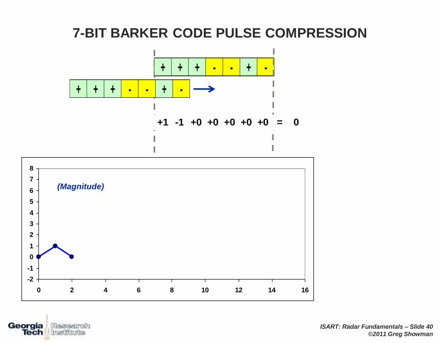
ISART: Radar Fundamentals – Slide 40
©2011 Greg Showman
7-BIT BARKER CODE PULSE COMPRESSION
-2
-1
0
1
2
3
4
5
6
7
8
0 2 4 6 8 10 12 14 16
+ + + - - + -
+ + + - - + -
(Magnitude)
+1 -1 +0 +0 +0 +0 +0 = 0

ISART: Radar Fundamentals – Slide 41
©2011 Greg Showman
7-BIT BARKER CODE PULSE COMPRESSION
-2
-1
0
1
2
3
4
5
6
7
8
0 2 4 6 8 10 12 14 16
+ + + - - + -
+ + + - - + -
(Magnitude)
-1 +1 -1 +0 +0 +0 +0 = -1

ISART: Radar Fundamentals – Slide 42
©2011 Greg Showman
7-BIT BARKER CODE PULSE COMPRESSION
-2
-1
0
1
2
3
4
5
6
7
8
0 2 4 6 8 10 12 14 16
+ + + - - + -
+ + + - - + -
(Magnitude)
-1 -1 +1 +1 +0 +0 +0 = 0

ISART: Radar Fundamentals – Slide 43
©2011 Greg Showman
7-BIT BARKER CODE PULSE COMPRESSION
-2
-1
0
1
2
3
4
5
6
7
8
0 2 4 6 8 10 12 14 16
+ + + - - + -
+ + + - - + -
(Magnitude)
+1 -1 -1 -1 +1 +0 +0 = -1

ISART: Radar Fundamentals – Slide 44
©2011 Greg Showman
7-BIT BARKER CODE PULSE COMPRESSION
-2
-1
0
1
2
3
4
5
6
7
8
0 2 4 6 8 10 12 14 16
+ + + - - + -
+ + + - - + -
(Magnitude)
+1 +1 -1 +1 -1 -1 +0 = 0

ISART: Radar Fundamentals – Slide 45
©2011 Greg Showman
7-BIT BARKER CODE PULSE COMPRESSION
-2
-1
0
1
2
3
4
5
6
7
8
0 2 4 6 8 10 12 14 16
+ + + - - + -
+ + + - - + -
(Magnitude)
+1 +1 +1 +1 +1 +1 +1 = +7

ISART: Radar Fundamentals – Slide 46
©2011 Greg Showman
7-BIT BARKER CODE PULSE COMPRESSION
-2
-1
0
1
2
3
4
5
6
7
8
0 2 4 6 8 10 12 14 16
+ + + - - + -
+ + + - - + -
(Magnitude)
0 +1 +1 -1 +1 -1 -1 = 0

ISART: Radar Fundamentals – Slide 47
©2011 Greg Showman
7-BIT BARKER CODE PULSE COMPRESSION
-2
-1
0
1
2
3
4
5
6
7
8
0 2 4 6 8 10 12 14 16
+ + + - - + -
+ + + - - + -
(Magnitude)
0 +0 +1 -1 -1 -1 +1 = -1

ISART: Radar Fundamentals – Slide 48
©2011 Greg Showman
7-BIT BARKER CODE PULSE COMPRESSION
-2
-1
0
1
2
3
4
5
6
7
8
0 2 4 6 8 10 12 14 16
+ + + - - + -
+ + + - - + -
(Magnitude)
0 +0 +0 -1 -1 +1 +1 = 0

ISART: Radar Fundamentals – Slide 49
©2011 Greg Showman
7-BIT BARKER CODE PULSE COMPRESSION
-2
-1
0
1
2
3
4
5
6
7
8
0 2 4 6 8 10 12 14 16
+ + + - - + -
+ + + - - + -
(Magnitude)
0 +0 +0 +0 -1 +1 -1 = -1

ISART: Radar Fundamentals – Slide 50
©2011 Greg Showman
7-BIT BARKER CODE PULSE COMPRESSION
-2
-1
0
1
2
3
4
5
6
7
8
0 2 4 6 8 10 12 14 16
+ + + - - + -
+ + + - - + -
(Magnitude)
0 +0 +0 +0 +0 +1 -1 = 0

ISART: Radar Fundamentals – Slide 51
©2011 Greg Showman
7-BIT BARKER CODE PULSE COMPRESSION
-2
-1
0
1
2
3
4
5
6
7
8
0 2 4 6 8 10 12 14 16
+ + + - - + -
+ + + - - + -
(Magnitude)
0 +0 +0 +0 +0 +0 -1 = -1

ISART: Radar Fundamentals – Slide 52
©2011 Greg Showman
7-BIT BARKER CODE PULSE COMPRESSION
-2
-1
0
1
2
3
4
5
6
7
8
0 2 4 6 8 10 12 14 16
+ + + - - + -
+ + + - - + -
(Magnitude)
0 +0 +0 +0 +0 +0 +0 = 0

ISART: Radar Fundamentals – Slide 53
©2011 Greg Showman
Outline
Background and Range Measurement
SNR and the Matched Filter
Radar Range Equation
Detection in Noise
Pulse Compression
Multiple Pulses
Antenna Effects

ISART: Radar Fundamentals – Slide 54
©2011 Greg Showman
= Pulse Width
Tp = Inter-Pulse Period
= Pulse Repetition Interval (PRI)
fp = Pulse Repetition Frequency (PRF)
= 1/Tp
Td = Coherent dwell time
Pulsed Waveform Parameters
Tp
0 5 10 15 20 25 30 35 40 45 50 55 60 65 70 75
To = RF Carrier Period
f0 = Carrier frequency = 1/To
= Wavelength = cTo = c/fo
c = Speed of light in vacuum = 3x10⁸ m/s
T0
f0 = 1 GHz = .3 m
f0 = 10 GHz = .03 m
Td

ISART: Radar Fundamentals – Slide 55
©2011 Greg Showman
Noncoherent vs Coherent Radar
Noncoherent radar uses amplitude
only to process returns
Coherent radar uses both amplitude
and phase to process returns.
Duplexer
Doppler
Analyzer
Pulsed
Amplifier
Pulsed
Amplifier
Receiver
CW
Oscillator
Detector
Duplexer
Transmitter
Receiver Detector
Duplexer
Transmitter
Receiver Detector
Reference
oscillator
Non-coherent
Coherent
Specifically, radar uses
time variation of phase
to infer target motion.

ISART: Radar Fundamentals – Slide 56
©2011 Greg Showman
Notional Pulse-Doppler Radar Block Diagram
cos(2(f0-f1)t)
cos(2(f1)t)
)t(R4
c
)t(Rf4)t( 0
Duplexer
Pulse
Mod
Receiver
Protect
STALO
LPF
LPF
A/D
A/D
Signal
Processor
Data
Processor
RF DigitalIF Baseband
In-phase (I)
Quadrature (Q)
BPF
90o90o
))t(tfcos()t(A 02
)]t(sin[)t(A)t(sQ
•STALO and COHO remove carrier frequency, fc.
•Baseband is DC except for phase/amplitude
variation of target (plus noise).
)]t(cos[)t(A)t(sI
)tfcos(Pt 02
))t(tfcos()t(A 12
COHO
BPF

ISART: Radar Fundamentals – Slide 57
©2011 Greg Showman
RADAR RANGE EQUATION: Multiple-Pulse Energy-to-Noise-Density Ratio
2 2
3 40 04
t d
s
P dT GE
N R L kT F
Presumes coherent integration
Extend pulswidth to
CPI integration time Td
But reduce by the TX duty factor d = /Tp

ISART: Radar Fundamentals – Slide 58
©2011 Greg Showman
RADAR RANGE EQUATION: Multiple-Pulse Energy-to-Noise-Density Ratio
2 22 2
3 34 40 0 0
2 2
3 4
0
4 4
4
avg dt d
s s
t
s
P G TPdG TE
N R L kT F R L kT F
P G n
R L kT F
Variations
Pavg is average TX power
n = number of pulses coherently integrated

ISART: Radar Fundamentals – Slide 59
©2011 Greg Showman
Motivations for Coherent Integration
(Doppler Processing)
Efficient increase in target SNR
Ability to measure range rate
Separation (by Doppler frequency) of ground clutter and moving targets
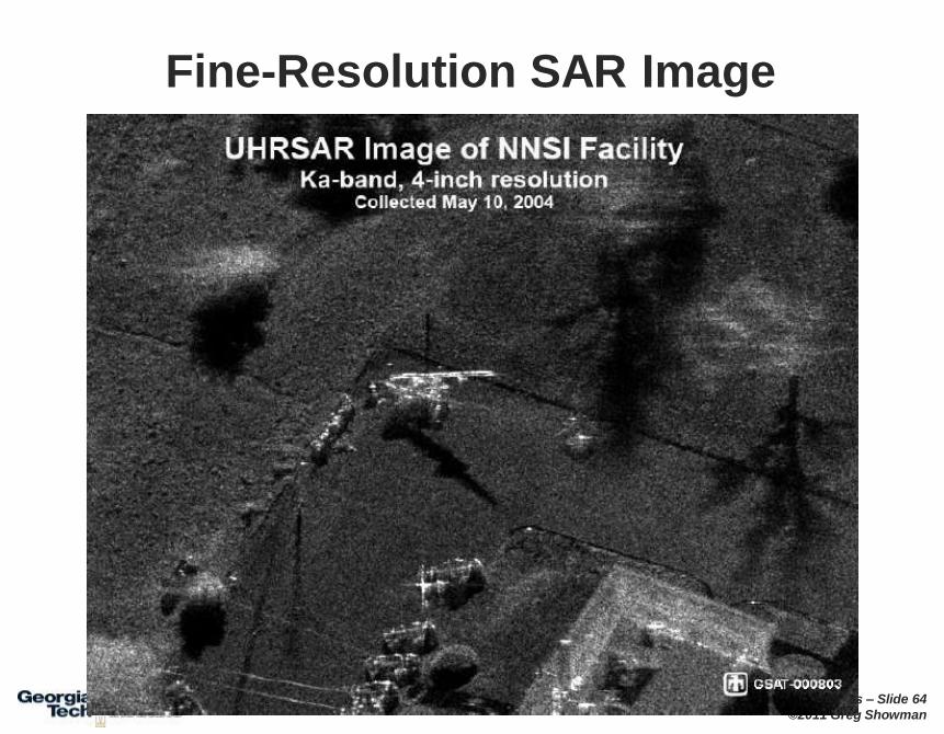
Fine-resolution imaging via SAR and ISAR

ISART: Radar Fundamentals – Slide 60
©2011 Greg Showman
Pulse-Doppler Waveform Concept
Maritime Radar -- Use of Doppler Frequency
1 2 3 4 KK-1K-2
1 2 3 NN-1N-24
1 2 3 4 M-2 M-1 M
Maritime Radar -- Use of Doppler Frequency
1 2 3 4 KK-1K-2
1 2 3 NN-1N-24
1 2 3 4 M-2 M-1 M
Pulse 1
Pulse M
Collect digital
I/Q samples
from each of N
range gates for
M pulses.
For each of N range
gates, perform M-point
FFT to obtain Doppler
spectrum.
Maritime Radar -- Use of Doppler FrequencyN
Ran
ge
M Doppler
Coherent pulse train
of M pulses.
PRI
Maritime Radar -- Use of Doppler Frequency
1 2 3 4 KK-1K-2
1 2 3 NN-1N-24
1 2 3 4 M-2 M-1 M
M filters for RG 1
(etc.)
1 2 3 4 MM-1M-2

ISART: Radar Fundamentals – Slide 61
©2011 Greg Showman
Air-to-Air Range-Doppler Maps

ISART: Radar Fundamentals – Slide 62
©2011 Greg Showman
GMTI Range-Doppler Map
Example of a 64-pulse GMTI range-Doppler map
Note substantial exo-clutter extent (boxes) for moving target detection
(Courtesy Raythoen Corporation)

ISART: Radar Fundamentals – Slide 63
©2011 Greg Showman
Range-Doppler Map
Example of a DBS range-Doppler map
DBS (Doppler Beam Sharpening) is a crude form of SAR
Note small exo-clutter extent
(Courtesy Raythoen Corporation)
ISART: Radar Fundamentals – Slide 64
©2011 Greg Showman
Fine-Resolution SAR Image

ISART: Radar Fundamentals – Slide 65
©2011 Greg Showman
Outline
Background and Range Measurement
SNR and the Matched Filter
Radar Range Equation
Detection in Noise
Pulse Compression
Multiple Pulses
Antenna Effects

ISART: Radar Fundamentals – Slide 66
©2011 Greg Showman
Antenna Gain and Area W
H
Azimuth beamwidth
Elevation
beamwidth
Antenna gain
WAZ
q
HEL
q
2
A4
H/W/
4G
Antenna
Area A=W H
Large antennas provide
High gain on TX
Large collection area on RX
Low energy on TX to other users outside the mainbeam
Reduced power on RX from sidelobe returns
Improved angle resolution against multiple targets
Increased angle measurement accuracy on one target
ISART: Radar Fundamentals – Slide 67
©2011 Greg Showman
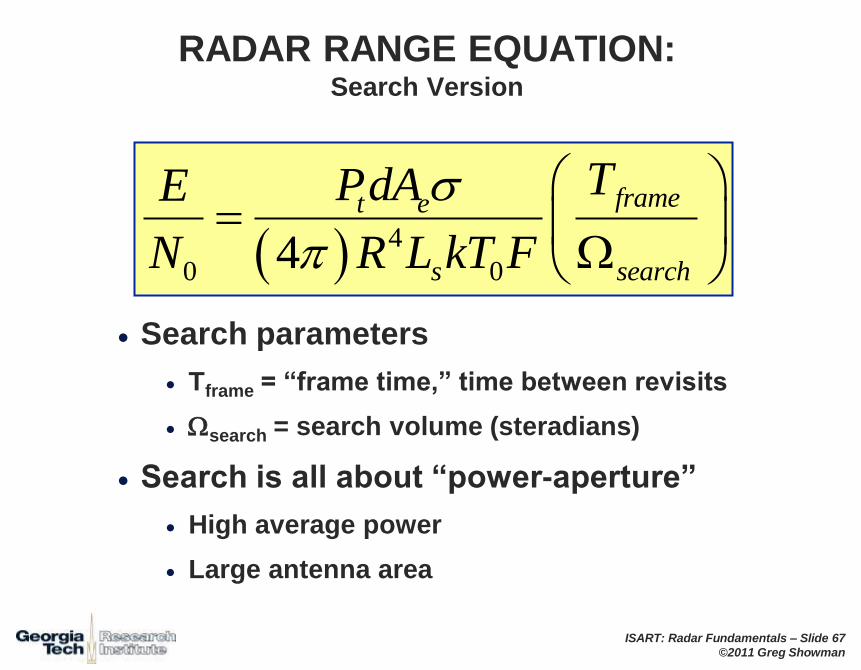
RADAR RANGE EQUATION: Search Version
4
0 04
framet e
s search
TPdAE
N R L kT F
Search parameters
Tframe = “frame time,” time between revisits
search = search volume (steradians)
Search is all about “power-aperture”
High average power
Large antenna area

ISART: Radar Fundamentals – Slide 68
©2011 Greg Showman
Outline
Background and Range Measurement
SNR and the Matched Filter
Radar Range Equation
Detection in Noise
Pulse Compression
Multiple Pulses
Antenna Effects