Is

Ca

b

c

a

ARR1A

KISIRWBP

1

ifmpfboeibtnptso

0d

Journal of Neuroscience Methods 187 (2010) 171–182

Contents lists available at ScienceDirect

Journal of Neuroscience Methods

journa l homepage: www.e lsev ier .com/ locate / jneumeth

ntrinsic signal optical imaging of brain function usinghort stimulus delivery intervals

ynthia H. Chen-Beea,∗, Teodora Agoncilloa, Christopher C. Laya,c, Ron D. Frostiga,b,c

Department of Neurobiology and Behavior, 2205 McGaugh Hall, University of California, Irvine, CA 92697-4550, United StatesDepartment of Biomedical Engineering, University of California, Irvine, CA 92697-4550, United StatesCenter for the Neurobiology of Learning and Memory, University of California, Irvine, CA 92697-4550, United States

r t i c l e i n f o

rticle history:eceived 6 October 2009eceived in revised form5 December 2009ccepted 8 January 2010

eywords:ntrinsic signal optical imagingtimulus delivery interval

a b s t r a c t

Intrinsic signal optical imaging (ISOI) can be used to map cortical function and organization. Because itsdetected signal lasts 10+ s consisting of three phases, trials are typically collected using a long (tens of sec-onds) stimulus delivery interval (SDI) at the expense of efficiency, even when interested in mapping onlythe first signal phase (e.g., ISOI initial dip). It is unclear how the activity profile can change when stimuliare delivered at shorter intervals, and whether a short SDI can be implemented to improve efficiency.The goals of the present study are twofold: characterize the ISOI activity profile when multiple stimuliare delivered at 4 s intervals, and determine whether successful mapping can be attained from trialscollected using an SDI of 4 s (offering >10× increase in efficiency). Our results indicate that four stimuli

nterstimulus intervalathisker

arrelrimary somatosensory cortex

delivered 4 s apart evoke an activity profile different from the triphasic signal, consisting of signal dips ina series at the same frequency as the stimuli despite a strong rise in signal prior to the 2nd to 4th stimuli.Visualization of such signal dips is dependent on using a baseline immediately prior to every stimulus.Use of the 4-s SDI is confirmed to successfully map activity with a similar location in peak activity andincreased areal extent and peak magnitude compared to using a long SDI. Additional experiments wereperformed to begin addressing issues such as SDI temporal jittering, response magnitude as a function

icatio

of SDI duration, and appl

. Introduction

The functional imaging technique intrinsic signal optical imag-ng (ISOI; Grinvald et al., 1986; Frostig et al., 1990; Ts’o et al., 1990;or a recent review see Frostig and Chen-Bee, 2009) using red illu-

ination is commonly employed for mapping cortical activity andlays an important role in furthering our understanding of brainunction and organization. The detected ISOI signal evoked by arief stimulus is slow in onset (within half a second of stimulusnset), long in duration (10+ s), and, at least in the rat (Chen-Beet al., 2007), is comprised of three signal phases consisting of a dipn signal below baseline followed by an overshoot in signal aboveaseline and another dip below baseline (referred to hereafter ashe initial dip, overshoot, and undershoot). Capture of the entire sig-al is not necessary; rather, the ISOI initial dip is better suited and

referentially exploited for successful ISOI mapping of brain func-ion. While typically not serving any mapping purpose, the latterignal phases are still taken into consideration; long intervals (tensf seconds) between stimulus deliveries are typically employed in

∗ Corresponding author. Tel.: +1 949 824 5031; fax: +1 949 824 2447.E-mail address: cbee@uci.edu (C.H. Chen-Bee).

165-0270/$ – see front matter © 2010 Elsevier B.V. All rights reserved.oi:10.1016/j.jneumeth.2010.01.009

n for successful mapping of cortical function topography.© 2010 Elsevier B.V. All rights reserved.

order to allow not just the ISOI initial dip but also any remain-ing ISOI signal phases to return to baseline. Such practice is at theexpense of data collection efficiency, substantially slowing the rateat which trials can be accumulated and hence undesirably prolong-ing an experiment; also, the occurrence of stimulus deliveries isconsiderably sparse compared to the stimulation experienced byawake and behaving subjects. We wondered whether the stimulusdelivery interval (SDI) could be shortened as a means to improvedata collection efficiency (as well as offer progress towards a regi-men of stimulus deliveries more analogous to behaviorally relevantstimulation). For example, rather than wait tens of seconds untilcompletion of the entire preceding signal, a given stimulus couldbe delivered after completion of only the preceding signal’s initialdip, which would require just a few seconds but would be at the riskof coinciding stimulus delivery with lingering signal. At present, theprofile of ISOI activity is unknown when a series of multiple stim-uli are delivered at short intervals; furthermore, it is also unclearwhether trial collection using a short SDI can be successfully used

for ISOI mapping of brain function.

Thus, the goals of the current study are twofold. We used ISOIto image brain activity in the rat barrel cortex evoked by brief (1 s)stimulation of a single whisker and addressed two questions. First,to investigate the consequences of delivering a stimulus without

1 roscie

wcawomltransetSf

o(

2

ia

2

ptCoababc

TS

Is6tr

72 C.H. Chen-Bee et al. / Journal of Neu

aiting for the entire completion of previously evoked signal, weharacterized the activity profile of four stimuli delivered 4 s aparts compared to a single stimulus delivery. Second, to determinehether a short SDI can be employed for successful ISOI mapping

f brain activity, within the same subject we compared the activityap obtained from collecting 128 trials using a short (4 s) versus

ong (tens of seconds) SDI. Additional experiments were performedo begin addressing the temporal jittering of the short SDI, theesponse magnitude as a function of SDI duration, and the actualpplication of the short SDI for successfully fulfilling the mappingeeds of an imaging study. The collective results of the presenttudy indicate that multiple stimuli delivered at 4 s intervals canvoke an activity profile with stereotypical properties differenthan the triphasic activity profile, and trial collection using a shortDI of 4 s can indeed be used for successful ISOI mapping of brainunction with substantial improvement in efficiency.

The subset of the present data acquired using a long SDI is partf a large data pool presented elsewhere in a previous publicationChen-Bee et al., 2007).

. Materials and methods

Most of the surgical preparation, imaging, and data analysis usedn the present study are described in detail elsewhere (Chen-Bee etl., 2007). Summary and additional details are provided below.

.1. Subjects and surgical preparation

Principles of laboratory animal care were followed, and allerformed procedures were in compliance with the National Insti-utes of Health guidelines and approved by the University ofalifornia Irvine Animal Care and Use Committee. At the startf an experiment, each adult male Sprague–Dawley rat received

bolus intraperitoneal injection of sodium pentobarbital (Nem-

utal, 55 mg/kg b.w.) followed by an intramuscular injection oftropine (0.05 mg/kg b.w.) into the hind leg. Supplemental Nem-utal injections were administered as necessary to maintain mildorneal reflexes and additional atropine injections were adminis-

able 1ummary of experiment details.

COLUMN 1 COLUMN 2Long SDIWith Jitter(stim + control trials)

Short SDINo Jitter

See Fig. 1A See Fig. 7A

Sample size (n) 10 ratsSingle trial 15-s trials 3-s trialsparameters 150 frames/trial 30 frames/trialStimulus delivery

(whisker C2)Single (5 deflectionsat 5 Hz for 1 s)

Single

Stimulus deliverybegan 1.5 s from startof stimulation trial

Stimulus deliverybegan 1.5 s from startof stimulation trial

Interval between endof one trial andstart of next trial

Average of 6 s,ranging randomlybetween 1 and 11 s

Exactly 1 s

Stimulus deliveryinterval (SDI)

Centered at 42 s Exactly 4 s

SDI jitter range >20 s 0 s (no jitter)Data collection

duration100 min to complete128 stim trials

10 min to complete128 stim trials

n all experiments, trials were collected with intrinsic signal optical imaging (ISOI) of rource. A CCD camera was used to capture frames at 10 Hz rate (i.e., 100-ms frames). Tria4 trials for Column 5), and the summed data collapsed into 500-ms frames to increase thhe different experimental conditions (shaded row). For all experiments, data analysis enelative to pre-stimulus data (see Fig. 1B). See text for details.

nce Methods 187 (2010) 171–182

tered every 6 h. Body temperature was monitored and maintainedat 37 ◦C with an electric homeothermic blanket. The exposed leftskull overlying the subregion of primary somatosensory cortexresponsive to the large facial whiskers was thinned to ∼150 �mthickness with a dental drill, and a saline-filled well of petroleumjelly sealed with a coverslip was built over the thinned skull region(Masino et al., 1993).

2.2. ISOI data acquisition

Each rat was placed under a 12-bit CCD camera combinedwith an inverted 50 mm lens such that a cortical region of6.5 mm × 4.9 mm beneath the thinned skull region mapped ontoa final array of 191 × 144 pixels (i.e., 1 pixel = 34 �m × 34 �m corti-cal region). An image of the surface vasculature was taken for laterreference (Fig. 7B) using green illumination before the CCD camerawas focused 600 �m below the cortical surface. For data collec-tion, the imaged region was continuously illuminated with a redlight-emitting diode (635 nm max, 15 nm full width at half-height)powered by a 6 V battery. During each imaging trial, frames werecaptured at 10 Hz rate (i.e., 100-ms frames). A single stimulus deliv-ery consisted of five rostral–caudal deflections at 5 Hz delivered toa single whisker (C2). Additional details about stimulus deliveryand trial collection are provided below according to experimen-tal condition. With noted exceptions, a total of 128 stimulationtrials were collected per experimental condition. At the end ofeach experiment, trials were separated according to condition andthen summed, and the summed data collapsed into 500-ms frames(referred to hereafter as a data file) to increase the signal-to-noiseratio.

2.3. Experimental design 1—activity profile for multiple stimulidelivered at 4 s intervals

To characterize the activity profile for multiple stimulus deliv-eries separated by a short interval, imaging was performed in twogroups of rats. For the first group (n = 10 rats), activity evoked by asingle stimulus was imaged (Fig. 1A) using trial collection parame-

COLUMN 3 COLUMN 4 COLUMN 5Long SDIWith Jitter (stimtrials only)

Extended trials Short SDIWith Jitter

See Fig. 3A

10 rats 8 rats 3 rats15-s trials 30-s trials 2-s trials150 frames/trial 300 frames/trial 20 frames/trialSingle 4-Stimuli series (four

single stimulusdeliveries 4 s apart)

Single

Stimulus deliverybegan 1.5 s from startof stimulation trial

4-Stimuli seriesbegan 1.5 s from startof stimulation trial

Stimulus deliverybegan 1.5 s from startof stimulation trial

Average of 6 s,ranging randomlybetween 1 and 11 s

Average of 6 s,ranging randomlybetween 1 and 11 s

Average of 2 s,ranging randomlybetween 1 and 3 s

Centered at 21 s (not applicable) Centered at 4 s

10 s 2 s50 min to complete128 stim trials

(not relevant) 5 min to complete 64stim trials

at barrel cortex (∼6.5 mm × 5 mm) using a red (635 nm wavelength) illuminationls were summed to achieve a total of 128 trials per experimental condition (excepte signal-to-noise ratio. Note the difference in the SDI and SDI jitter range between

tailed the conversion of post-stimulus 500-ms frames into fractional change values

C.H. Chen-Bee et al. / Journal of Neuroscience Methods 187 (2010) 171–182 173

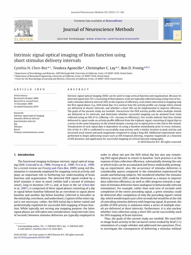
Fig. 1. Single stimulus delivery and trial collection using a long SDI (stim + control trials). (A) Schematic of trial accumulation. Trial collection parameters are detailed inTable 1, Column 1. Because an equal number of control trials were collected, stimulus delivery intervals (SDIs) were in essence centered at 42 s with a jitter range of 20+ s.One stimulation trial is enlarged to illustrate the temporal relationship between stimulus delivery and the 500-ms frames (dark streaks depict large dural and cortical surfaceblood vessels). (B) Schematic of visualizing intrinsic signal activity. Post-stimulus frames are converted to fractional change (FC) values relative to pre-stimulus data. Fordetails see Section 2; grayscale bar applies to all applicable figures. (C) Visualization and plot of intrinsic signal activity for a representative rat. A single stimulus delivery usinga onsetf urse f

tpd(aueuTTw

long SDI evoked a triphasic signal. Activity was relatively stable prior to stimulusrom blood vessels (light or dark streaks). The post-stimulus intrinsic signal time co

ers as detailed in Table 1, Column 1 (because of the trial collectionarameters, the average interval between consecutive stimuluseliveries was in the order of tens of seconds). For the second groupn = 8 rats), activity evoked by a series of four stimuli delivered 4 spart (referred to hereafter as 4-stimuli series) was imaged (Fig. 3A)sing extended imaging trials as detailed in Table 1, Column 4. The

xperiment day began with a quick confirmation that a single stim-lus evoked a typical ISOI triphasic signal (all details same as inable 1, Column 3, except only 64 stimulation trials were collected).hen, for the experiment proper, extended trials were collected inhich the 4-stimuli series was delivered in each trial. The extended

, evidenced by a homogeneous pre-stimulus image with only subtle contributionsrom the location of peak initial dip activity was extracted and plotted.

trial duration enabled the continuous capture, and therefore char-acterization, of activity throughout the delivery of the 4-stimuliseries and for 15.5 s thereafter (Fig. 3A). The interval between thestimuli within the 4-stimuli series was set to 4 s because trial col-lection using a short SDI of 4 s would permit data collection at asubstantially accelerated rate while still ensuring that a given stim-

ulus delivery occurred after termination of the preceding ISOI initialdip. Also, a 4 s interval was a good candidate for revealing potentialconsequences of coinciding a given stimulus delivery with the lattersegment of the preceding evoked signal because the ISOI overshootphase maximizes approximately 4 s after stimulus onset (see Fig. 2).

174 C.H. Chen-Bee et al. / Journal of Neuroscience Methods 187 (2010) 171–182

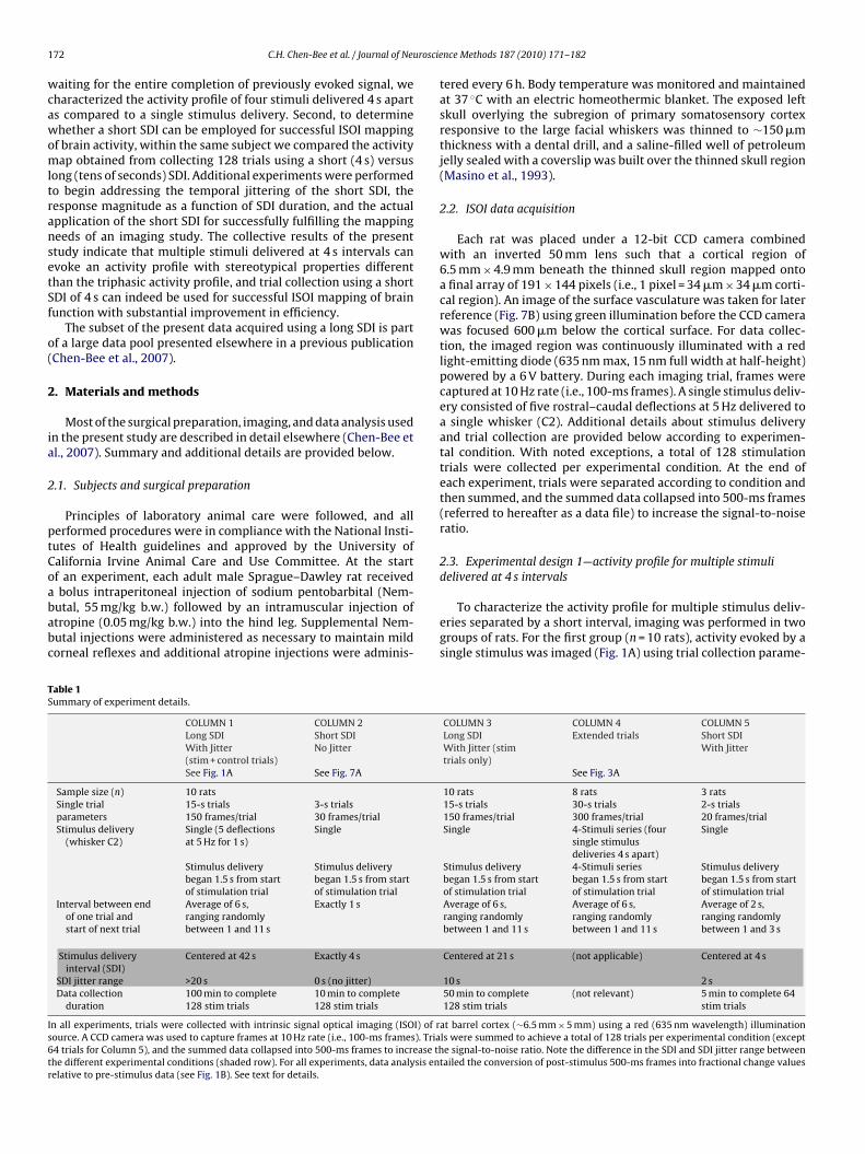
F trials)o g. 1C.o

2u

dStAicatrtuceutse

2

p

ig. 2. Single stimulus delivery and trial collection using a long SDI (stim + controlf the triphasic intrinsic signal are provided for 10 rats. First rat is the same as in Finset.

.4. Experimental design 2—activity map from trial collectionsing a long versus short SDI

The imaging of activity evoked by a single stimulus delivery asescribed above for the first group of rats (n = 10) involved a longDI (Fig. 1A; Table 1, Column 1) and thus the data were also usedo provide mapping results from trials collected using a long SDI.dditional imaging was performed on this group of rats as detailed

n Table 1, Column 2 (Fig. 7A) to provide mapping results from trialsollected using a short SDI. The long SDI was in essence centeredt 42 s with a >20 s jitter range because an equal number of con-rol trials were interleaved with stimulation trials; ∼100 min wereequired to complete 128 stimulation trials. It should be notedhat employment of a long SDI with jittering, where both stim-lation and control trials are collected, is an example of what isommonly practiced in ISOI experiments. The short SDI was set toxactly 4 s (hence, no jitter) to be congruent to the 4-stimuli seriessed in the experiments described above; <10 min were requiredo complete 128 stimulation trials. Trial blocks using a long ver-us short SDI were interleaved in random order throughout thexperiment.

.5. Data analysis

Data files were analyzed for visualization, quantification, andlotting of pre- and post-stimulus intrinsic signal activity.

—summary of 10 rats. Visualization and average plot (means and standard errors)Note that on average the overshoot signal peaked approximately 4 s after stimulus

2.5.1. VisualizationPost-stimulus activity was visualized as described in detail else-

where (Chen-Bee et al., 1996, 2000, 2007). Briefly, fractional change(FC) values for a given post-stimulus 500-ms frame were calculatedrelative to the 500-ms frame collected immediately prior to stimu-lus onset (baseline frame) on a pixel-by-pixel basis (Fig. 1B). For the4-stimuli series data files, the 500-ms frame immediately prior tostim 1 of the series served as the baseline frame. Then, to generateimages of post-stimulus activity, an 8-bit linear grayscale mappingfunction was applied to the FC values, with an FC value of 0 (nochange from baseline) mapped to middle gray shade and an arbi-trary threshold of ±2.5 × 10−4 FC (±0.025%) from 0 used such thatevoked ISOI initial dip (also ISOI undershoot) and ISOI overshootsignal phase would appear as black or white, respectively, in gener-ated images (Fig. 1B). The same method was applied for visualizingpre-stimulus activity except that FC values were calculated for the500-ms frame immediately prior to stimulus delivery relative tothe frame immediately prior to it.

2.5.2. Quantification and plottingFor the pre-stimulus data, the median FC value was used as a

measure of average pre-stimulus activity. For the post-stimulusdata, the FC values obtained from averaging the 2nd and 3rd500-ms post-stimulus frames were used for quantifying the arealextent, absolute peak magnitude, and peak location of the ISOI ini-tial dip. Prior to quantification, the post-stimulus FC values were

C.H. Chen-Bee et al. / Journal of Neuroscience Methods 187 (2010) 171–182 175

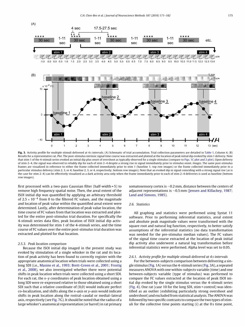
Fig. 3. Activity profile for multiple stimuli delivered at 4 s intervals. (A) Schematic of trial accumulation. Trial collection parameters are detailed in Table 1, Column 4. (B)Results for a representative rat. Plot. The post-stimulus intrinsic signal time course was extracted and plotted at the location of peak initial dip evoked by stim 1 delivery. Notethat stim 1 of the 4-stimuli series evoked an initial dip plus onset of overshoot as typically observed for a single stimulus (compare to Figs. 1C plot and 2 plot). Upon deliveryof stim 2–4, the signal was observed to reliably dip for each of stim 2–4 despite a strong rise in signal immediately prior to stimulus onset. Images. The same post-stimulusf r to stp row it n ther

firIoadtt4ice

2

etalesFlScsal

rames are visualized in reference to either the frame collected immediately prioarticular stimulus delivery (stim 2, 3, or 4; baseline 2, 3, or 4, respectively; bottomhe case for stim 2–4) can be effectively visualized as a dark activity area only wheow images).

rst processed with a two-pass Gaussian filter (half-width = 5) toemove high frequency spatial noise. Then, the areal extent of theSOI initial dip was quantified by applying an arbitrary thresholdf 2.5 × 10−4 from 0 to the filtered FC values, and the magnitudend location of peak value within the quantified areal extent wereetermined. Lastly, after determination of peak value location, theime course of FC values from that location was extracted and plot-ed for the entire post-stimulus trial duration. For specifically the-stimuli series data files, peak location of ISOI initial dip activ-

ty was determined for stim 1 of the 4-stimuli series, and the timeourse of FC values over the entire post-stimulus trial duration wasxtracted and plotted for that location.

.5.3. Peak location comparisonBecause the ISOI initial dip imaged in the present study was

voked by stimulation of a single whisker in the rat and its loca-ion of peak activity has been found to correctly register with theppropriate anatomical location when trials were collected using aong SDI (i.e., Masino et al., 1993; Brett-Green et al., 2001; Frostigt al., 2008), we also investigated whether there were potentialhifts in peak location when trials were collected using a short SDI.or each rat, the x–y coordinates of peak location obtained using aong SDI were re-expressed relative to those obtained using a short

DI such that a relative coordinate of (0,0) would indicate perfecto-localization, and shifts along the x-axis or y-axis would indicatehifts in peak location along the rostral–caudal or medial–lateralxis, respectively (see Fig. 7G). It should be noted that the radius of aarge whisker’s anatomical representation (or barrel) in rat primary

im 1 (baseline 1; top row images) or the frame collected immediately prior to amages). Note that an evoked dip in signal coinciding with a strong signal rise (as isframe immediately prior to each of stim 2–4 deliveries is used as baseline (bottom

somatosensory cortex is ∼0.2 mm, distance between the centers ofadjacent representations is ∼0.5 mm (Jensen and Killackey, 1987;Land and Simons, 1985).

2.6. Statistics

All graphing and statistics were performed using Systat 11software. Prior to performing inferential statistics, areal extentand absolute peak magnitude values were transformed with thesquare root and natural log function, respectively, to better satisfyassumptions of the inferential statistics (no data transformationwas needed for the pre-stimulus median values). The FC valuesof the signal time course extracted at the location of peak initialdip activity also underwent a natural log transformation beforeinferential statistics were performed. Alpha level was set to 0.05.

2.6.1. Activity profile for multiple stimuli delivered at 4 s intervalsFor the between-subjects comparison between delivering a sin-

gle stimulus (Fig. 1A) versus the 4-stimuli series (Fig. 3A), a repeatedmeasures ANOVA with one within-subjects variable (time) and onebetween-subjects variable (type of stimulus) was performed tocompare the FC values extracted at the location of peak ISOI ini-tial dip evoked by the single stimulus versus the 4-stimuli series

(Fig. 4). One rat (case 10 for the long SDI, stim + control) was iden-tified as an outlier (exhibiting particularly strong overshoot andundershoot) and excluded from statistical analysis. The ANOVA wasfollowed by two specific contrasts to compare the two types of stim-uli for the collective time points starting (i) at the 0 s time point,

176 C.H. Chen-Bee et al. / Journal of Neuroscience Methods 187 (2010) 171–182

Fig. 4. Activity profile evoked by a single stimulus using a long SDI versus the 4-stimuli series. Plotted here is the average signal time course (means and standard error bars)for a single stimulus delivery using a long SDI (open circle; same plot as in Fig. 2) versus the 4-stimuli series (filled circle). For the collective time points of 0 up until the4 s time point (stim 2 onset), no significant difference in signal time course was found between the two types of stimulus deliveries (F = 0.21, p = 0.656), indicating thats rshood s (F(1,1

s circle

ctdpuansao

2S

cwe

3

3d

2aoaa4firsupsFfi2

pas

tim 1 of the 4-stimuli series evoked an initial dip and beginning portion of the oveifference was found for the collective time points starting at 4.5 s up through 6.0timulus using a long SDI (open circle) stim 2 delivery induced a dip in signal (filled

orresponding to the delivery onset of both the single stimulus andhe 4-stimuli series, up until the time point corresponding to theelivery onset of stim 2 of the 4-stimuli series; these collective timeoints spanned a time epoch when there was no difference in stim-lation between the two types of stimuli; or (ii) 4.5 up through 6.0 s,time epoch where the greatest difference in ISOI overshoot sig-al was observed in response to delivery of stim 2 of the 4-stimulieries as compared to a single stimulus. Bonferroni correction waspplied to account for multiple contrasts, for an adjusted alpha levelf 0.05/2 = 0.025.

.6.2. Activity map from trial collection using a long versus shortDI

For the within-subjects comparison of mapping results for trialollection using a long versus short SDI, two-tailed paired t-testsere performed on the pre-stimulus median, transformed areal

xtent, and transformed peak magnitude values (Fig. 7D–F).

. Results

.1. Experimental design 1—activity profile for multiple stimulielivered at 4 s intervals

As expected based on our previous findings (Chen-Bee et al.,007), a single stimulus (Fig. 1A; Table 1, Column 1) reliably evokedtriphasic signal spanning 10+ s (plots in Figs. 1 and 2) consistingf an ISOI initial dip (visualized as a black coherent area in gener-ted images) followed by an ISOI overshoot (white area) and thenn ISOI undershoot (second black area). In contrast, delivery of the-stimuli series (Fig. 3A; Table 1, Column 4) evoked a signal pro-le with markedly different temporal properties. Results from aepresentative case are provided in Fig. 3B. Stim 1 of the 4-stimulieries evoked an ISOI initial dip similarly to that for a single stim-lus using a long SDI (compare stim 1 of Fig. 3B plot, with Fig. 2lot), presumably due to the long interval (17.5–27.5 s) betweentim 1 of one series and stim 4 of the preceding series (see Fig. 3A).urthermore, initiation of stim 1’s ISOI overshoot signal was con-rmed along with the coinciding of this strong overshoot with stim

delivery at the 4.0 s time point (Fig. 3B plot).

Upon stim 2 delivery, the signal was observed to dip (Fig. 3Blot) in a manner similar for stim 1 and for a single stimulus usinglong SDI (Fig. 2 plot), despite a strong rise in signal just prior to

tim 2 onset. A repeated measures ANOVA performed on the signal

(1,15)

t comparable to that for a single stimulus using a long SDI. In contrast, a significant5) = 9.83, p = 0.007; asterisk), where compared to the overshoot evoked by a single). Note that stim 3–4 deliveries also each induced a dip in signal (filled circle).

time course (Fig. 4) found a significant interaction (F(26,390) = 11.95,p = 1 × 10−15) between type of stimulus (4-stimuli series vs. single)and trial time point. Specifically, no significant difference betweenstimulus type was found for the collective time points starting at 0 sup until onset of stim 2 delivery (F(1,15) = 0.21, p = 0.656). In contrast,a significant difference was found for the collective time pointsstarting at 4.5 s up through 6.0 s, corresponding to those time pointswith the greatest dip in signal upon stim 2 delivery (F(1,15) = 9.83,p = 0.007), indicating that the signal dip observed just after stim2 onset was due specifically to stim 2 delivery. Complementaryresults were obtained for stim 3–4: a strong rise in signal prior tostimulus delivery followed by a dip in signal after stimulus delivery(Fig. 4, filled circles). The collective results demonstrated the abil-ity of stim 2–4 to exert a dip in signal despite a rise in signal priorto their deliveries. Interestingly, another dip in signal occurred 4 safter stim 4 onset even though no more stimuli were being deliv-ered (Fig. 4, filled circles). In summary, multiple stimuli delivered atshort intervals (as is the case for the 4-stimuli series) each success-fully evoked a signal dip, for a final activity profile that consistedof multiple signal dips occurring in a series at the same frequencyas the stimulus deliveries (Fig. 4, filled circles) and that collectivelyconstitute an activity profile different from the triphasic activityprofile associated with a single stimulus (Fig. 4, open circles).

The reliable signal dips described above must be due to suc-cessful evoking of ISOI initial dips. We found that successfulvisualization of such signal dips was dependent on the baselineframe used for generating images. When the frame immediatelyprior to stim 1 onset was used as baseline (baseline 1), the gener-ated images (Fig. 3B, top row images) were able to visualize stim 1’ssignal dip (dark activity area) and onset of overshoot (white activityarea) similarly to that for a single stimulus delivery (Fig. 2 images),but were unable to effectively visualize signal dips superimposedon signal rises as was the case for stim 2–4. In contrast, by using asbaseline the frame captured immediately prior to each delivery ofstim 2–4 (i.e., baseline 2 for stim 2, baseline 3 for stim 3, etc.; seeFig. 3B plot), the generated images were finally able to visualize thesignal dips of stim 2–4 as dark activity areas in a manner similar tostim 1 and to a single stimulus delivery, areas that exhibited com-

parable peak magnitude and areal extent except with increased‘white’ vessel activity. (Also, the frame immediately prior to stim2–4 appeared relatively homogeneous with some increased ‘white’vessel activity.) Note the use of a baseline prior to each of stim 2-4was analogous to baseline 1 for stim 1, as well as for the baseline

C.H. Chen-Bee et al. / Journal of Neuroscience Methods 187 (2010) 171–182 177

F 0 ratse . 3B. F

fa

tbism

3u

dcrahaieiw

ig. 5. Activity profile for multiple stimuli delivered at 4 s intervals—summary of 1voked by the 4-stimuli series are provided for 10 rats. First rat is the same as in Fig

rame used for single stimulus delivery. See Fig. 5 for summary ofll cases.

The results of Figs. 3–5 collectively suggested that trial collec-ion using a short SDI of 4 s can be successfully employed to maprain activity, as long as data analysis utilized a baseline captured

mmediately prior to each stimulus delivery. Results from the nextet of experiments were obtained to explicitly confirm the imple-entation of such mapping.

.2. Experimental design 2—activity maps from trial collectionsing a long versus short SDI

The ISOI initial dip results for a single stimulus delivery asescribed above were used to provide mapping results from trialollection using a long SDI (centered at 42 s with a >20-s jitterange; Fig. 1A; Table 1, Column 1). Besides the reliable evoking oftriphasic signal (Fig. 2 images), pre-stimulus data were relativelyomogeneous across the imaged region, as supported by minimal

ctivity observed from large surface blood vessels (subtle streaks inmages) and an average FC value of 0.2 × 10−4 (or∼10×weaker thanvoked signal; compare Fig. 7D and E). (The ISOI initial dip exhib-ted the same signal properties when control trials were excluded,

hich entailed the use of an SDI that was sufficiently long but

. Average plot (means and standard errors) and visualization of the activity profileor details see Fig. 3 legend.

reduced by half and therefore provided a 2× increase in efficiency;Fig. 6). Mapping results from trial collection using a short SDI (cen-tered at 4 s with no jitter; Table 1, Column 2) were also obtainedfrom the same animals (Fig. 7A). Except for some increased ‘white’vessel presence in images, pre-stimulus data appeared quite simi-lar for the short SDI (Fig. 7B and C) and no significant difference wasfound for the average pre-stimulus FC values (Fig. 7D; two-tailedpaired t(9) = −0.20, p = 0.847). In contrast, differences in the evokedISOI initial dip were found. The ISOI initial dip images for the shortSDI contained some increased ‘white’ vessel presence (Fig. 7B andC) similarly observed for the pre-stimulus data, and the peak mag-nitude (Fig. 7E; two-tailed paired t(9) = 3.50, p = 0.007) and arealextent (Fig. 7F; two-tailed paired t(9) = 3.23, p = 0.010) of the ISOIinitial dip were significantly increased. The ISOI initial dip peaklocations, however, were comparable as indicated by co-registrywithin 0.2 mm (approximate radius of a large whisker barrel) inhalf of the cases and 0.2–0.5 mm for the remaining cases (Fig. 7G).

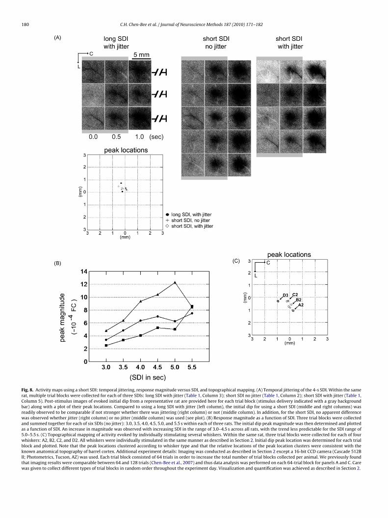
In additional experiments, we began to tackle the following

questions regarding the use of short SDIs for ISOI mapping ofbrain function: (1) is the increase in the initial dip peak magni-tude and areal extent observed for the short SDI due to a lack oftemporal jittering?; (2) how does the response amplitude changeacross a range of short SDIs?; and (3) can a short SDI be used to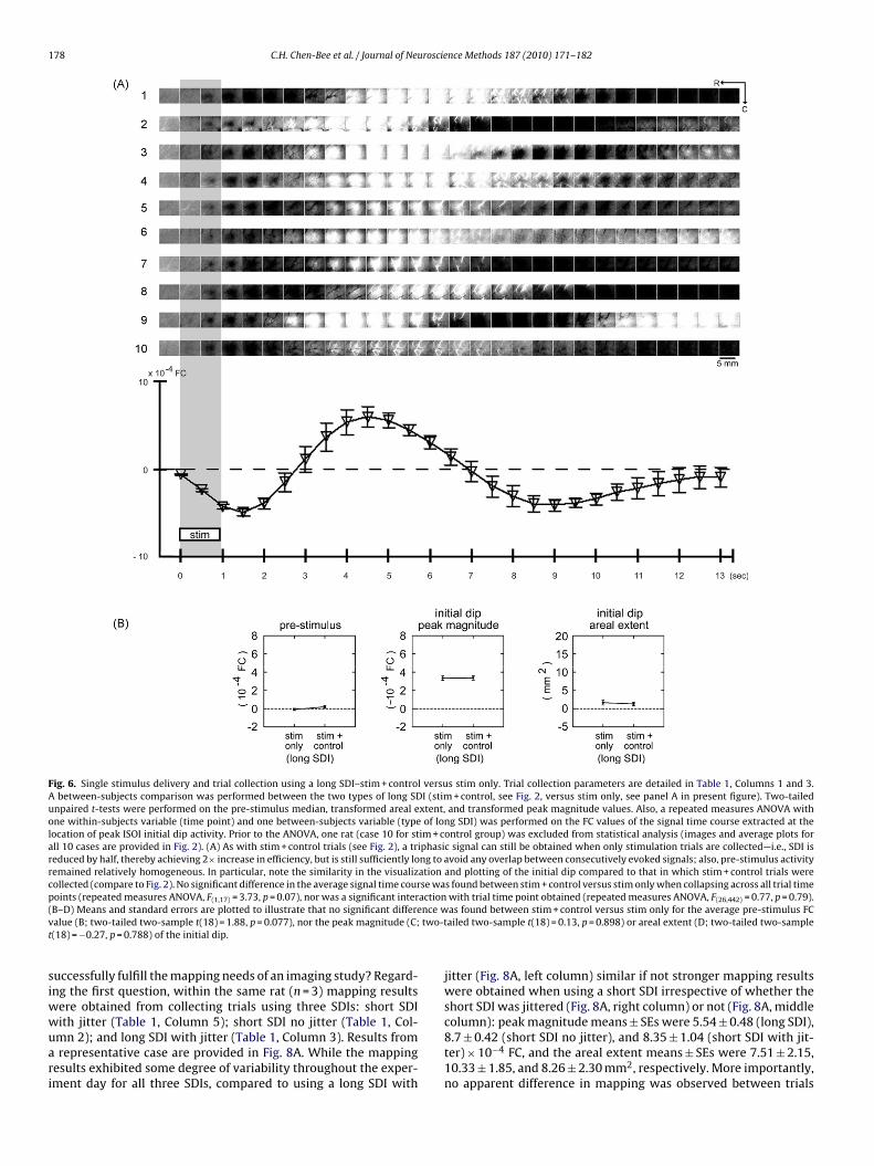

178 C.H. Chen-Bee et al. / Journal of Neuroscience Methods 187 (2010) 171–182

Fig. 6. Single stimulus delivery and trial collection using a long SDI–stim + control versus stim only. Trial collection parameters are detailed in Table 1, Columns 1 and 3.A between-subjects comparison was performed between the two types of long SDI (stim + control, see Fig. 2, versus stim only, see panel A in present figure). Two-tailedunpaired t-tests were performed on the pre-stimulus median, transformed areal extent, and transformed peak magnitude values. Also, a repeated measures ANOVA withone within-subjects variable (time point) and one between-subjects variable (type of long SDI) was performed on the FC values of the signal time course extracted at thelocation of peak ISOI initial dip activity. Prior to the ANOVA, one rat (case 10 for stim + control group) was excluded from statistical analysis (images and average plots forall 10 cases are provided in Fig. 2). (A) As with stim + control trials (see Fig. 2), a triphasic signal can still be obtained when only stimulation trials are collected—i.e., SDI isreduced by half, thereby achieving 2× increase in efficiency, but is still sufficiently long to avoid any overlap between consecutively evoked signals; also, pre-stimulus activityremained relatively homogeneous. In particular, note the similarity in the visualization and plotting of the initial dip compared to that in which stim + control trials werecollected (compare to Fig. 2). No significant difference in the average signal time course was found between stim + control versus stim only when collapsing across all trial timepoints (repeated measures ANOVA, F = 3.73, p = 0.07), nor was a significant interaction with trial time point obtained (repeated measures ANOVA, F = 0.77, p = 0.79).( nce wv two-tt

siwwuari

(1,17)

B–D) Means and standard errors are plotted to illustrate that no significant differealue (B; two-tailed two-sample t(18) = 1.88, p = 0.077), nor the peak magnitude (C;(18) = −0.27, p = 0.788) of the initial dip.

uccessfully fulfill the mapping needs of an imaging study? Regard-ng the first question, within the same rat (n = 3) mapping results

ere obtained from collecting trials using three SDIs: short SDI

ith jitter (Table 1, Column 5); short SDI no jitter (Table 1, Col-mn 2); and long SDI with jitter (Table 1, Column 3). Results fromrepresentative case are provided in Fig. 8A. While the mapping

esults exhibited some degree of variability throughout the exper-ment day for all three SDIs, compared to using a long SDI with

(26,442)

as found between stim + control versus stim only for the average pre-stimulus FCailed two-sample t(18) = 0.13, p = 0.898) or areal extent (D; two-tailed two-sample

jitter (Fig. 8A, left column) similar if not stronger mapping resultswere obtained when using a short SDI irrespective of whether theshort SDI was jittered (Fig. 8A, right column) or not (Fig. 8A, middle

column): peak magnitude means ± SEs were 5.54 ± 0.48 (long SDI),8.7 ± 0.42 (short SDI no jitter), and 8.35 ± 1.04 (short SDI with jit-ter) × 10−4 FC, and the areal extent means ± SEs were 7.51 ± 2.15,10.33 ± 1.85, and 8.26 ± 2.30 mm2, respectively. More importantly,no apparent difference in mapping was observed between trials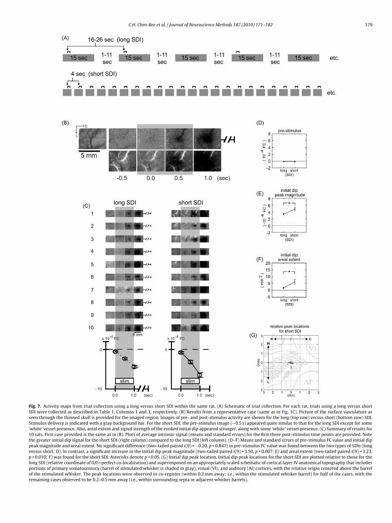

C.H. Chen-Bee et al. / Journal of Neuroscience Methods 187 (2010) 171–182 179

Fig. 7. Activity maps from trial collection using a long versus short SDI within the same rat. (A) Schematic of trial collection. For each rat, trials using a long versus shortSDI were collected as described in Table 1, Columns 1 and 3, respectively. (B) Results from a representative case (same as in Fig. 1C). Picture of the surface vasculature asseen through the thinned skull is provided for the imaged region. Images of pre- and post-stimulus activity are shown for the long (top row) versus short (bottom row) SDI.Stimulus delivery is indicated with a gray background bar. For the short SDI, the pre-stimulus image (−0.5 s) appeared quite similar to that for the long SDI except for some‘white’ vessel presence. Also, areal extent and signal strength of the evoked initial dip appeared stronger, along with some ‘white’ vessel presence. (C) Summary of results for10 rats. First case provided is the same as in (B). Plots of average intrinsic signal (means and standard errors) for the first three post-stimulus time points are provided. Notethe greater initial dip signal for the short SDI (right column) compared to the long SDI (left column). (D–F) Means and standard errors of pre-stimulus FC value and initial dippeak magnitude and areal extent. No significant difference (two-tailed paired t(9) = −0.20, p = 0.847) in pre-stimulus FC value was found between the two types of SDIs (longversus short; D). In contrast, a significant increase in the initial dip peak magnitude (two-tailed paired t(9) = 3.50, p = 0.007; E) and areal extent (two-tailed paired t(9) = 3.23,p = 0.010; F) was found for the short SDI. Asterisks denote p < 0.05. (G) Initial dip peak location. Initial dip peak locations for the short SDI are plotted relative to those for thelong SDI (relative coordinate of 0,0 = perfect co-localization) and superimposed on an appropriately scaled schematic of cortical layer IV anatomical topography that includesportions of primary somatosensory (barrel of stimulated whisker is shaded in gray), visual (VI), and auditory (AI) cortices, with the relative origin centered above the barrelof the stimulated whisker. The peak locations were observed to co-register (within 0.2 mm away; i.e., within the stimulated whisker barrel) for half of the cases, with theremaining cases observed to be 0.2–0.5 mm away (i.e., within surrounding septa or adjacent whisker barrels).

180 C.H. Chen-Bee et al. / Journal of Neuroscience Methods 187 (2010) 171–182

Fig. 8. Activity maps using a short SDI: temporal jittering, response magnitude versus SDI, and topographical mapping. (A) Temporal jittering of the 4-s SDI. Within the samerat, multiple trial blocks were collected for each of three SDIs: long SDI with jitter (Table 1, Column 3); short SDI no jitter (Table 1, Column 2); short SDI with jitter (Table 1,Column 5). Post-stimulus images of evoked initial dip from a representative rat are provided here for each trial block (stimulus delivery indicated with a gray backgroundbar) along with a plot of their peak locations. Compared to using a long SDI with jitter (left column), the initial dip for using a short SDI (middle and right columns) wasreadily observed to be comparable if not stronger whether there was jittering (right column) or not (middle column). In addition, for the short SDI, no apparent differencewas observed whether jitter (right column) or no jitter (middle column) was used (see plot). (B) Response magnitude as a function of SDI. Three trial blocks were collectedand summed together for each of six SDIs (no jitter): 3.0, 3.5, 4.0, 4.5, 5.0, and 5.5 s within each of three rats. The initial dip peak magnitude was then determined and plottedas a function of SDI. An increase in magnitude was observed with increasing SDI in the range of 3.0–4.5 s across all rats, with the trend less predictable for the SDI range of5.0–5.5 s. (C) Topographical mapping of activity evoked by individually stimulating several whiskers. Within the same rat, three trial blocks were collected for each of fourwhiskers: A2, B2, C2, and D2. All whiskers were individually stimulated in the same manner as described in Section 2. Initial dip peak location was determined for each trialblock and plotted. Note that the peak locations clustered according to whisker type and that the relative locations of the peak location clusters were consistent with theknown anatomical topography of barrel cortex. Additional experiment details: Imaging was conducted as described in Section 2 except a 16-bit CCD camera (Cascade 512BII; Photometrics, Tucson, AZ) was used. Each trial block consisted of 64 trials in order to increase the total number of trial blocks collected per animal. We previously foundthat imaging results were comparable between 64 and 128 trials (Chen-Bee et al., 2007) and thus data analysis was performed on each 64-trial block for panels A and C. Carewas given to collect different types of trial blocks in random order throughout the experiment day. Visualization and quantification was achieved as described in Section 2.

roscie

wmtuAww5aqSftwfft

4

ptstdnegeiicb((sfeaneslmttsusa

sevrsradvss(i

C.H. Chen-Bee et al. / Journal of Neu

ith jittering or no jittering of the short SDI (Fig. 8A, right versusiddle column, respectively; graph). Regarding the second ques-

ion, within the same rat (n = 3) mapping results were obtainedsing six different SDIs (no jitter): 3.0, 3.5, 4.0, 4.5, 5.0, and 5.5 s.s illustrated in Fig. 8B, across the three rats the peak magnitudeas observed to increase as the SDI increased from 3.0 to 4.5 s,ith the trend becoming less predictable across the SDI range of

.0–5.5 s (increased contribution from large surface blood vesselslso seemed to increase with increasing SDI). Regarding the thirduestion, within the same rat (n = 1) mapping results using a shortDI of 4 s (no jitter) were obtained from individually stimulatingour different whiskers (A2, B2, C2, and D3). As illustrated in Fig. 8C,he relative locations of peak responses evoked by the stimulatedhiskers were consistent with the known anatomical topography

or those whiskers, indicating that the use of a short SDI can success-ully fulfill the mapping needs of an imaging study such as providinghe topographical map of barrel cortex.

. Discussion

Our findings indicate that the activity profile evoked by multi-le stimuli delivered at short intervals (4 s apart) is different fromhe triphasic signal associated with a single stimulus delivery, con-isting of multiple signal dips occurring at the same frequency ashe stimulus deliveries (Fig. 4). These successive signal dips occurespite the fact that they coincide with a strong rise in signal begin-ing with the second stimulus delivery (Figs. 3–5). They can beffectively visualized as dark activity areas as long as images areenerated using a baseline temporally local to each stimulus deliv-ry (Figs. 3B and 5), which in principle is analogous to how ISOInitial dip visualization is achieved when a single stimulus deliverys used (Figs. 2 and 6). Trial collection using a short SDI is explicitlyonfirmed as a viable option for mapping of ISOI initial dip. It cane successfully used to target the appropriate anatomical locationFig. 7G), and to map the peak magnitude (Fig. 7E) and areal extentFig. 7F). Mapping using a short SDI offers the advantage of sub-tantially increasing data collection efficiency (>10×). Furthermore,or the same number of collected trials (128), the mapping resultsxhibit an increased peak magnitude and areal extent (Fig. 7C, End F), thus offering the opportunity to reduce the number of trialseeded for effective brain mapping and thereby further increasingfficiency. Indeed, the present study provides several examples ofuccessful mapping achieved by reducing the total number of col-ected trials by half (down to 64 trials) while using an SDI of 4 s (a

ere 5 min to complete) to address such questions as the effect ofemporal jittering of the SDI (Fig. 8A), the response curve as a func-ion of SDI interval (Fig. 8B), and the topographical activity map ofeveral whiskers (Fig. 8C). Lastly, from a behavioral perspective, these of a short SDI offers progress towards employing a regimen oftimulus deliveries more akin to stimulation experienced by awakend behaving subjects.

Evoking and imaging of ISOI initial dip is possible when using ahort SDI under a condition as adverse as coinciding stimulus deliv-ry with a strong rise in signal (Figs. 3B, 4, and 5). To effectivelyisualize evoked ISOI initial dip as a dark activity area, however,equires the use of a baseline frame captured immediately prior totimulus onset (e.g., baseline 2, 3 or 4) rather than a more tempo-ally remote baseline (e.g., baseline 1; Fig. 3B), analogous to whenlong SDI is used. It should be noted that the same post-stimulusata can provide different information (attenuation in signal rise

isualized as a white activity area versus successful evoking of aignal dip visualized as a dark activity area that coincides with aignal rise) depending on the baseline frame used for visualizationbaseline 1 versus baseline 2, 3, or 4; Fig. 3B). The effective visual-zation of evoked ISOI initial dip despite such an adverse condition

nce Methods 187 (2010) 171–182 181

bodes well for ISOI mapping of brain function; if an ISOI initial dipcan be successfully evoked and mapped when it coincides with arise in signal, then it should also be the case when an ISOI initialdip is evoked during spontaneous fluctuations in activity knownto occur throughout the course of an experiment (Mayhew et al.,1996; Ferezou et al., 2006; Chen-Bee et al., 2007), as long as baselineused for analysis is captured immediately prior to stimulus onset. Itremains to be determined whether SDIs other than 4 s can providecomparable mapping of brain activity.

Successful ISOI mapping of brain activity does not depend onthe periodic nature of the short SDI. As illustrated in Fig. 8, compa-rable results are obtained irrespective of whether or not the shortSDI is jittered. At first glance, these results appear contradictory toresults of Dale, Bandettini, and their colleagues (Dale and Buckner,1997; Bandettini and Cox, 2000) using BOLD fMRI, albeit for theBOLD fMRI overshoot signal phase. As with ISOI, BOLD fMRI is ahemodynamic-based imaging technique that can be used to mapbrain function. Their collective results indicate SDI jitter is requiredfor successful mapping and it is argued that jittering is a means toovercome complications arising from overlapping of consecutiveovershoot signals. More specifically, because the overlap of BOLDfMRI overshoot signals increases with decreasing SDI duration, jit-tering is necessary for SDIs lasting just a few seconds but becomesless critical with longer SDIs (Dale, 1999; Bandettini and Cox, 2000;see also Chapter 9 by Huettel et al. (2008) on issues related to SDIjittering for successful BOLD fMRI detection and estimation of over-shoot signal). Our results (Fig. 8) can be explained along this lineof reasoning by taking into consideration that the ISOI initial dip isunder investigation here. Specifically, compared to the overshoot,the ISOI initial dip terminates several seconds sooner (Fig. 2) andthus to avoid overlap of consecutive signals should not require aslong of an SDI. In other words, an SDI of 4 s is sufficiently long andthus jittering is no longer necessary because overlap of ISOI initialdip signals has already been avoided. For mapping of specificallythe ISOI initial dip, it would be interesting to see to what extent theSDI needs to be shortened in order to necessitate jittering.

Our similarity in results irrespective of whether the short SDIis jittered (Fig. 8) offers two other implications. First, it specificallyconfirms that a short SDI can be implemented in a manner morecomparable to a long SDI (where jittering is commonly employed).Second, the greater peak magnitude and areal extent of ISOI initialdip signal observed when using a short SDI (Fig. 7B and C, E andF) cannot be easily explained as a strengthening of evoked activ-ity induced by the periodic evoking of signals because comparableresults are obtained with jittering (Fig. 8). Thus, for mapping ofspecifically the ISOI initial dip, unexpected strengthening of brainactivity need not be a concern when the short SDI is not jittered.If not due to the periodicity of evoked signals, then it remains tobe determined how to explain the observed increase in ISOI initialdip peak magnitude and areal extent. One possibility is that theincrease is simply indicative of the brain’s increased response to anincreased degree of stimulation (as achieved with an increased den-sity of stimulus deliveries per unit time), analogous to increasingmagnitude and areal extent of a single whisker functional rep-resentation with increasing stimulus amplitude (Petersen, 2003).Another possibility is that the increase is in some way benefittingfrom an elevated level of oxygenated blood present during stimulusdeliveries, as suggested by the rise in signal prior to each delivery ofstim 2–4 as compared to stim 1 (Figs. 3B and 4). Future research isneeded to understand the underlying neuronal and hemodynamicmechanisms contributing to our observed increase in ISOI initial

dip signal when using short SDI, as well as how the ISOI initial dipproperties may change with changes in underlying mechanismsacross a range of short SDIs. Nevertheless, such future elucidationneed not preclude the use of a short SDI as a viable option for ISOImapping of brain function.

1 roscie

adlts5toltdmadatitn

4

aofawbtaamcKSmosetebeaobisEo–dmfpSs(tjtiuT

relates with previous optical imaging using intrinsic signals. Magn Reson Med

82 C.H. Chen-Bee et al. / Journal of Neu

Finally, the increase in ISOI initial dip peak magnitude (Fig. 7E)nd areal extent (Fig. 7F) indicates that these activity attributes areependent on the interval of the SDI, but may not be the case for

ocation of peak activity (Fig. 7G). Based on a small sample size ofhree rats, it would appear that the signal strength increases as thehort SDI increases from 3.0–4.5 s (results were less predictable for.0–5.5 s; Fig. 8B). Further research is needed to determine whetherhis trend is upheld. Therefore, accounting for the exact intervalf the short SDI may be less critical when using ISOI mapping forocalization purposes (i.e., targeting of peak or overall activity loca-ion). The short SDI should be taken into account, however, whenetailed mapping of activity involves direct comparison in peakagnitude and/or areal extent, especially as the underlying mech-

nisms of the imaged signal have the potential to differ in theirynamics. Interestingly, when evoked signals are sufficiently farpart, no difference is observed in peak magnitude or areal extent ofhe ISOI initial dip even when the interval between evoked signalss reduced by half (Fig. 6B). Thus, beyond some maximum value,he peak magnitude and areal extent of the ISOI initial dip is likelyo longer dependent on the SDI interval.

.1. General implications

In the present study, the reliable evoking of signal dips in seriest 4 s intervals is explicitly confirmed, as well as the collectingf trials using a short SDI for successful ISOI mapping of brainunction with substantially faster acquisition time. A Fourier-basedpproach is another means for achieving faster acquisition time,hich improves the signal-to-noise ratio by effectively filtering out

iological noise, and is optimal for imaging cortical functional sys-ems that are innately cyclic and continuous such as orientationnd ocular dominance columns but is less suitable for non-cyclicnd non-continuous systems such as whisker representations orore complex and abstract systems represented in higher corti-

al areas (see Kalatsky and Stryker, 2003, recently reviewed byalatsky, 2009). Needless to say, deciding on the interval of theDI for a particular ISOI study requires careful consideration of theany parameters relevant to that study (e.g., type and duration

f stimulus delivery; animal model; spatiotemporal properties ofignal evoked by a single stimulus delivery; signal phase of inter-st; data analysis algorithms; etc.). Our results suggest, however,hat irrespective of the parameter space, shorter SDIs (not nec-ssarily 4 s) are an option worth considering for ISOI mapping ofrain function in vivo, even at the risk of overlapping consecutivelyvoked signals to such a degree as coinciding stimulus delivery withsegment of the previously evoked signal that is strong and in thepposite direction as the signal of interest. Of course, the SDI cane shortened to the point that it prevents the simultaneous imag-

ng of multiple ISOI signal phases and thus would not be useful fortudies interested in characterizing the entire ISOI triphasic signal.ffective visualization of evoked signal – especially when the signalf interest is a transient change occurring on top of a larger signalrequires the use of a baseline that is temporally local to stimuluselivery (e.g., immediately prior to stimulus onset). The use of aore temporally remote baseline, however, can also provide use-

ul information such as confirming whether a change in signal isresent during stimulus deliveries. Determination of the optimalDI should begin with the characterization of the entire evokedignal in response to a single stimulus delivery using a long SDIas is the case in the present study). Depending on the total dura-ion of the evoked signal of interest, the optimal SDI may require

ittering. When multiple SDIs are being considered, standardizinghe SDI may be less relevant when mapping is performed for local-zation purposes, but becomes more critical when shorter SDIs aresed for characterizing peak magnitude and areal extent of maps.he increased peak magnitude and areal extent observed in the

nce Methods 187 (2010) 171–182

present study introduces the possibility that short SDIs might offersome benefit for BOLD fMRI mapping of its initial dip (Menon et al.,1995).

In conclusion, signal dips can be reliably evoked in a series at 4 sintervals and trials can be collected using a 4-s SDI for successfulISOI mapping of brain function, providing a substantial improve-ment in data collection efficiency and thus offering the opportunityto dramatically increase the number of research questions that canbe addressed within the same imaging experiment (case in point,our mapping of activity evoked by individually stimulating fourdifferent whiskers or using six different SDIs within the same rat).

Acknowledgments

We thank S. Soo and C. Wah for assistance with data analysis,and M. Davis for proofreading a previous version of the manuscript.This work was supported by the NIH-NINDS NS-43165, NS-48350,and NS-055832.

References

Bandettini PA, Cox RW. Event-related fMRI contrast when using constant interstim-ulus interval: theory and experiment. Magn Reson Med 2000;43:540–8.

Brett-Green BA, Chen-Bee CH, Frostig RD. Comparing the functional representationsof central and border whiskers in rat primary somatosensory cortex. J Neurosci2001;21:9944–54.

Chen-Bee CH, Agoncillo T, Xiong Y, Frostig RD. The triphasic intrinsic signal: impli-cations for functional imaging. J Neurosci 2007;27:4572–86.

Chen-Bee CH, Kwon MC, Masino SA, Frostig RD. Areal extent quantification of func-tional representations using intrinsic signal optical imaging. J Neurosci Methods1996;68:27–37.

Chen-Bee CH, Polley DB, Brett-Green B, Prakash N, Kwon MC, Frostig RD. Visualizingand quantifying evoked cortical activity assessed with intrinsic signal imaging.J Neurosci Methods 2000;97:157–73.

Dale AM. Optimal experimental design for event-related fMRI. Hum Brain Mapp1999;8:109–14.

Dale AM, Buckner RL. Selective aceraging of rapidly presented individual trials usingfMRI. Human Brain Mapping 1997;5:329–40.

Ferezou I, Bolea S, Petersen CC. Visualizing the cortical representation ofwhisker touch: voltage-sensitive dye imaging in freely moving mice. Neuron2006;50:617–29.

Frostig RD, Chen-Bee CH. Visualizing adult cortical plasticity using intrinsic signaloptical imaging. In: Frostig RD, editor. In vivo optical imaging of brain function.2-nd ed. Boca Raton: CRC Press; 2009.

Frostig RD, Lieke EE, Ts’o DY, Grinvald A. Cortical functional architecture and localcoupling between neuronal activity and the microcirculation revealed by invivo high-resolution optical imaging of intrinsic signals. Proc Natl Acad Sci USA1990;87:6082–6.

Frostig RD, Xiong Y, Chen-Bee CH, Kvasnak E, Stehberg J. Large-scale organization ofrat sensorimotor cortex based on a motif of large activation spreads. J Neurosci2008;28:13274–84.

Grinvald A, Lieke E, Frostig RD, Gilbert CD, Wiesel TN. Functional architectureof cortex revealed by optical imaging of intrinsic signals. Nature 1986;324:361–4.

Huettel SA, Song AW, McCartny G. Functional magnetic resonance imaging. seconded. Sunderland, MA: Sinauer Associates; 2008.

Jensen KF, Killackey HP. Terminal arbors of axons projecting to the somatosensorycortex of the adult rat. II. The altered morphology of thalamocortical afferentsfollowing neonatal infraorbital nerve cut. J Neurosci 1987;7:3544–53.

Kalatsky VA. Fourier approach to optical imaging. In: Frostig RD, editor. In vivooptical imaging of brain function. Boca Raton: CRC Press; 2009.

Kalatsky VA, Stryker MP. New paradigm for optical imaging: temporally encodedmaps of intrinsic signal. Neuron 2003;38:529–45.

Land PW, Simons DJ. Cytochrome oxidase staining in the rat SmI barrel cortex. JComp Neurol 1985;238:225–35.

Masino SA, Kwon MC, Dory Y, Frostig RD. Characterization of functional organizationwithin rat barrel cortex using intrinsic signal optical imaging through a thinnedskull. Proc Natl Acad Sci USA 1993;90:9998–10002.

Mayhew JE, Askew S, Zheng Y, Porrill J, Westby GW, Redgrave P, et al. Cerebralvasomotion: a 0.1-Hz oscillation in reflected light imaging of neural activity.Neuroimage 1996;4:183–93.

Menon RS, Ogawa S, Hu X, Strupp JP, Anderson P, Ugurbil K. BOLD based functionalMRI at 4 Tesla includes a capillary bed contribution: echo-planar imaging cor-

1995;33:453–9.Petersen CC. The barrel cortex—integrating molecular, cellular and systems physi-

ology. Pflugers Arch 2003;447:126–34.Ts’o DY, Frostig RD, Lieke EE, Grinvald A. Functional organization of primate visual

cortex revealed by high resolution optical imaging. Science 1990;249:417–20.