Intraday Trading Invariants for Equity-Index Futures · Intraday Trading Invariants for...
29
Intraday Trading Invariants for Equity-Index Futures Torben G. Andersen, Oleg Bondarenko, Albert S. Kyle and Anna Obizhaeva Fields Institute Toronto, Canada January 2015 Andersen, Bondarenko, Kyle, and Obizhaeva Intraday Invariance 1/29
Transcript of Intraday Trading Invariants for Equity-Index Futures · Intraday Trading Invariants for...
Intraday Trading Invariantsfor Equity-Index Futures
Torben G. Andersen, Oleg Bondarenko, Albert S. Kyle andAnna Obizhaeva
Fields InstituteToronto, Canada
January 2015
Andersen, Bondarenko, Kyle, and Obizhaeva Intraday Invariance 1/29
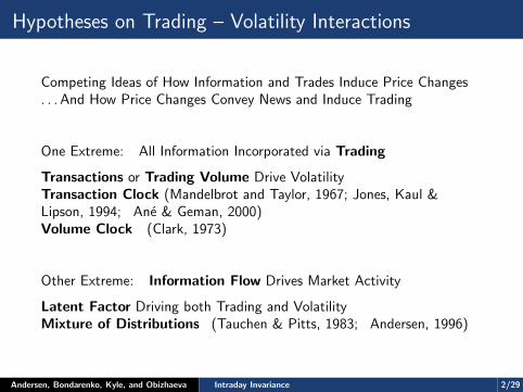
Hypotheses on Trading – Volatility Interactions
Competing Ideas of How Information and Trades Induce Price Changes. . . And How Price Changes Convey News and Induce Trading
One Extreme: All Information Incorporated via Trading
Transactions or Trading Volume Drive VolatilityTransaction Clock (Mandelbrot and Taylor, 1967; Jones, Kaul &Lipson, 1994; Ane & Geman, 2000)Volume Clock (Clark, 1973)
Other Extreme: Information Flow Drives Market Activity
Latent Factor Driving both Trading and VolatilityMixture of Distributions (Tauchen & Pitts, 1983; Andersen, 1996)
Andersen, Bondarenko, Kyle, and Obizhaeva Intraday Invariance 2/29
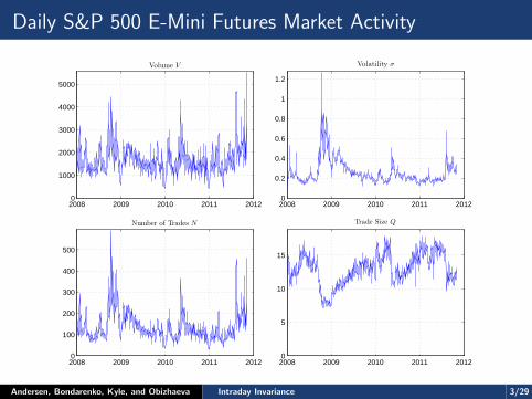
Daily S&P 500 E-Mini Futures Market Activity
2008 2009 2010 2011 20120
1000
2000
3000
4000
5000
Volume V
2008 2009 2010 2011 20120
100
200
300
400
500
Number of Trades N
2008 2009 2010 2011 20120
0.2
0.4
0.6
0.8
1
1.2
Volatility σ
2008 2009 2010 2011 20120
5
10
15
Trade Size Q
Andersen, Bondarenko, Kyle, and Obizhaeva Intraday Invariance 3/29
Hypotheses on Trading – Volatility Interactions
Focus typically on Observations at Daily Level
Exception: Ane & Geman, 2000; Near Tick-by-Tick
But Nobody has been Able to Confirm their Results
We also Fail to Verify Hypothesis
Use High-Frequency Data to Explore Interactions
Include Market Microstructure “Invariance” in Analysis
Empirical Support for Invariance via Diverse Market Phenomena
Major Expansion in Realm of Features Covered by Invariance
Andersen, Bondarenko, Kyle, and Obizhaeva Intraday Invariance 4/29
Why High-Frequency Analysis
Fact: Pronounced Intraday Market Activity Patterns
News Incorporated into Prices quickly; Trading Fast
Huge Systematic Variation over 24-Hour Trading Day
Does any Basic Regularity Apply in this Setting?
Macroeconomic Announcements particular Challenge
Large Price Jump on Impact without (much) Trading
Subsequent Price Discovery Process
Sudden Market Turmoil: Crisis, Flash Crash
Do Same or Different Regularities Apply in this Context?
Andersen, Bondarenko, Kyle, and Obizhaeva Intraday Invariance 5/29
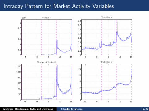
Intraday Pattern for Market Activity Variables
−5 0 5 10 150
0.5
1
1.5
2
2.5
3
x 104
Volume V
−5 0 5 10 150
200
400
600
800
1000
1200
Number of Trades N
−5 0 5 10 150
0.1
0.2
0.3
0.4
0.5
0.6
0.7
0.8
Volatility σ
−5 0 5 10 150
5
10
15
20
25
Trade Size Q
Andersen, Bondarenko, Kyle, and Obizhaeva Intraday Invariance 6/29
S&P 500 E-Mini Futures Market
Sample: BBO Files from CME Group; Jan 4, 2008 – Nov 2, 2011
Among World’s Most Active Markets – Price Discovery for Equities
Time Stamped to Second; Sequenced in Actual Order
Using Front Month Contract until Week before Expiration (most Liquid)
Three Daily Regimes: Asia, Europe, North America
Sunday – Thursday 17:15 – 2:00; 2:00-8:30; 8:30 – 15:15
Andersen, Bondarenko, Kyle, and Obizhaeva Intraday Invariance 7/29
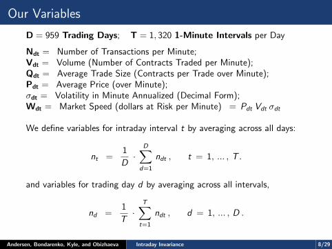
Our Variables
D = 959 Trading Days; T = 1, 320 1-Minute Intervals per Day
Ndt = Number of Transactions per Minute;Vdt = Volume (Number of Contracts Traded per Minute);Qdt = Average Trade Size (Contracts per Trade over Minute);Pdt = Average Price (over Minute);σdt = Volatility in Minute Annualized (Decimal Form);Wdt = Market Speed (dollars at Risk per Minute) = Pdt Vdt σdt
We define variables for intraday interval t by averaging across all days:
nt =1
D·
D∑d=1
ndt , t = 1, ... , T .
and variables for trading day d by averaging across all intervals,
nd =1
T·
T∑t=1
ndt , d = 1, ... , D .
Andersen, Bondarenko, Kyle, and Obizhaeva Intraday Invariance 8/29
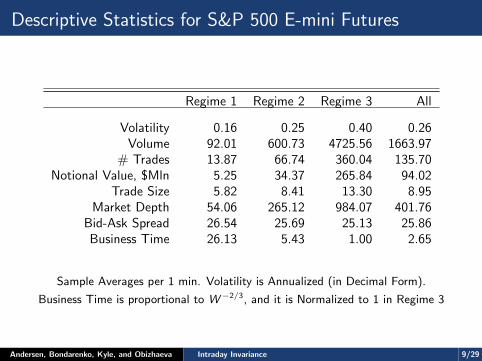
Descriptive Statistics for S&P 500 E-mini Futures
Regime 1 Regime 2 Regime 3 All
Volatility 0.16 0.25 0.40 0.26Volume 92.01 600.73 4725.56 1663.97
# Trades 13.87 66.74 360.04 135.70Notional Value, $Mln 5.25 34.37 265.84 94.02
Trade Size 5.82 8.41 13.30 8.95Market Depth 54.06 265.12 984.07 401.76
Bid-Ask Spread 26.54 25.69 25.13 25.86Business Time 26.13 5.43 1.00 2.65
Sample Averages per 1 min. Volatility is Annualized (in Decimal Form).
Business Time is proportional to W−2/3, and it is Normalized to 1 in Regime 3
Andersen, Bondarenko, Kyle, and Obizhaeva Intraday Invariance 9/29
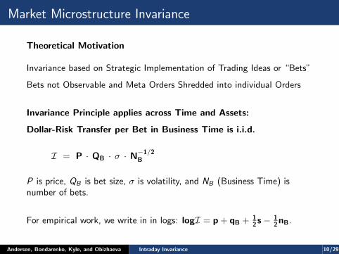
Market Microstructure Invariance
Theoretical Motivation
Invariance based on Strategic Implementation of Trading Ideas or “Bets”
Bets not Observable and Meta Orders Shredded into individual Orders
Invariance Principle applies across Time and Assets:
Dollar-Risk Transfer per Bet in Business Time is i.i.d.
I = P · QB · σ · N−1/2B
P is price, QB is bet size, σ is volatility, and NB (Business Time) isnumber of bets.
For empirical work, we write in in logs: logI = p + qB + 12 s− 1
2 nB.
Andersen, Bondarenko, Kyle, and Obizhaeva Intraday Invariance 10/29
Market Microstructure Invariance
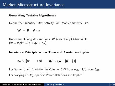
Generating Testable Hypotheses
Define the Quantity “Bet Activity” or “Market Activity” W ,
W = P · V · σ
Under simplifying Assumptions, W (essentially) Observable(w = logW = p + qB + nB)
Invariance Principle across Time and Assets now implies:
nB ∼ 23 w and qB ∼ 1
3 w − [p + 12 s]
For Same (σ,P), Variation in Volume: 2/3 from NB , 1/3 from QB .
For Varying (σ,P), specific Power Relations are Implied
Andersen, Bondarenko, Kyle, and Obizhaeva Intraday Invariance 11/29
Market Microstructure Invariance
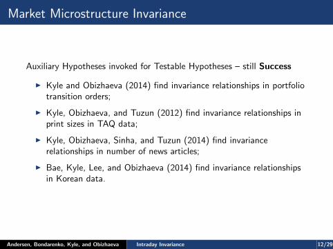
Auxiliary Hypotheses invoked for Testable Hypotheses – still Success
I Kyle and Obizhaeva (2014) find invariance relationships in portfoliotransition orders;
I Kyle, Obizhaeva, and Tuzun (2012) find invariance relationships inprint sizes in TAQ data;
I Kyle, Obizhaeva, Sinha, and Tuzun (2014) find invariancerelationships in number of news articles;
I Bae, Kyle, Lee, and Obizhaeva (2014) find invariance relationshipsin Korean data.
Andersen, Bondarenko, Kyle, and Obizhaeva Intraday Invariance 12/29
Invariance Inspired Predications
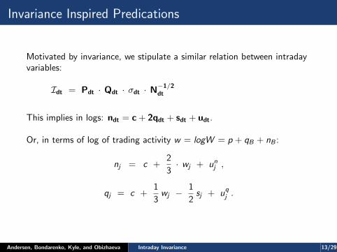
Motivated by invariance, we stipulate a similar relation between intradayvariables:
Idt = Pdt · Qdt · σdt · N−1/2dt
This implies in logs: ndt = c + 2qdt + sdt + udt.
Or, in terms of log of trading activity w = logW = p + qB + nB :
nj = c +2
3· wj + unj ,
qj = c +1
3wj −
1
2sj + uqj .
Andersen, Bondarenko, Kyle, and Obizhaeva Intraday Invariance 13/29

Suggestive Test for Alternative Theories
V and Q implicitly included within W ( = PVσ = PQNσ ).
Ignoring P, Relation σ2dt ∼ Vdt implies sdt = c + ndt + qdt .
Ignoring P, Relation σ2dt ∼ Ndt implies sdt = c + ndt .
nj = c + 23
[wj − 3
2 qj
]+ un
j . [Clark]and
nj = c + 23 [ wj − qj ] + un
j . [Ane & Geman]and
nj = c + 23 [ wj ] + un
j . [Invariance]
In terms of the nested specification:
sj − nj = c + β · qj + uqj .
where β = 1 (Clark), β = 0 (Ane-Geman), or β = −2 (invariance).
Andersen, Bondarenko, Kyle, and Obizhaeva Intraday Invariance 14/29
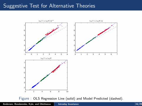
Suggestive Test for Alternative Theories
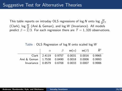
This table reports on intraday OLS regressions of logN onto log WQ3/2
(Clark), log WQ (Ane & Geman), and logW (Invariance). All models
predict β = 2/3. For each regression there are T = 1, 320 observations.
Table : OLS Regression of logN onto scaled logW
α β se(α) se(β) R2
Clark 2.4119 0.9757 0.0031 0.0016 0.9965Ane & Geman 1.7538 0.8490 0.0018 0.0006 0.9993
Invariance 0.8579 0.6708 0.0033 0.0007 0.9986
Andersen, Bondarenko, Kyle, and Obizhaeva Intraday Invariance 15/29
Suggestive Test for Alternative Theories
−1 0 1 2 3 4 5 6
2
3
4
5
6
7
logN vs logW/Q3/2
0 1 2 3 4 5 6 7
2
3
4
5
6
7
logN vs logW/Q
0 2 4 6 8 10
2
3
4
5
6
7
logN vs logW
Figure : OLS Regression Line (solid) and Model Predicted (dashed).
Andersen, Bondarenko, Kyle, and Obizhaeva Intraday Invariance 16/29
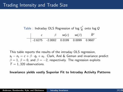
Trading Intensity and Trade Size
Table : Indraday OLS Regression of log σ2
N onto logQ
c β se(c) se(β) R2
-2.6275 -2.0002 0.0199 0.0099 0.9687
This table reports the results of the intraday OLS regression,st − nt = c + β · qt + ut . Clark, Ane & Geman and invariance predictβ = 1, β = 0, and β = −2, respectively. The regression exploitsT = 1, 320 observations.
Invariance yields vastly Superior Fit to Intraday Activity Patterns
Andersen, Bondarenko, Kyle, and Obizhaeva Intraday Invariance 17/29
Trading Intensity and Trade Size
1 1.5 2 2.5 3 3.5
−9
−8
−7
−6
−5
logσ2/N vs logQ
1 1.5 2 2.5 3 3.5
−9
−8
−7
−6
−5
logσ2/N vs logQ
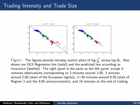
Figure : The figures provide intraday scatter plots of log σ2
Ntversus logQt . Also
shown are OLS Regression line (solid) and the predicted line according toinvariance (dashed). The right panel is the same as the left panel, except itremoves observations corresponding to 3 minutes around 1:00, 3 minutesaround 2:00 (start of the European regime), 3+30 minutes around 8:30 (start ofRegime 3 and the 9:00 announcements), and 16 minutes at the end of trading.
Andersen, Bondarenko, Kyle, and Obizhaeva Intraday Invariance 18/29
Intraday Invariance and Macro Announcements
Overall Invariance yields vastly Superior Fit to Intraday ActivityPatterns
Extremes? Macro Announcements Involve Dramatic Spikes
7:30 CT: Employment, CPI, PPI, Retail Sales, Housing Starts, . . .
9:00 CT: Home Sales, Confidence Survey, Factory Orders . . .
Andersen, Bondarenko, Kyle, and Obizhaeva Intraday Invariance 19/29
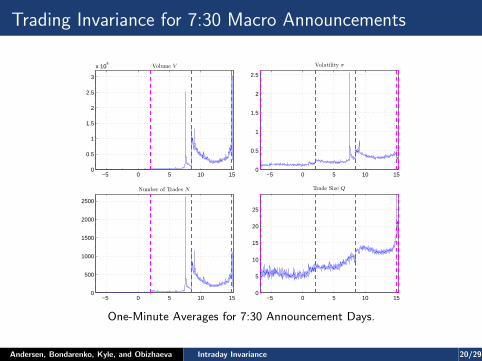
Trading Invariance for 7:30 Macro Announcements
−5 0 5 10 150
0.5
1
1.5
2
2.5
3
x 104
Volume V
−5 0 5 10 150
0.5
1
1.5
2
2.5
Volatility σ
−5 0 5 10 150
500
1000
1500
2000
2500
Number of Trades N
−5 0 5 10 150
5
10
15
20
25
Trade Size Q
One-Minute Averages for 7:30 Announcement Days.
Andersen, Bondarenko, Kyle, and Obizhaeva Intraday Invariance 20/29
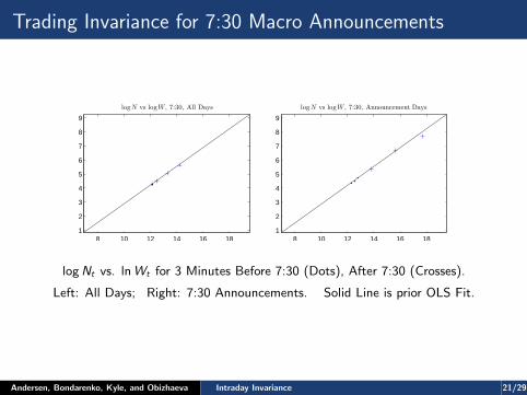
Trading Invariance for 7:30 Macro Announcements
8 10 12 14 16 181
2
3
4
5
6
7
8
9
logN vs logW , 7:30, All Days
8 10 12 14 16 181
2
3
4
5
6
7
8
9
logN vs logW , 7:30, Announcement Days
logNt vs. lnWt for 3 Minutes Before 7:30 (Dots), After 7:30 (Crosses).
Left: All Days; Right: 7:30 Announcements. Solid Line is prior OLS Fit.
Andersen, Bondarenko, Kyle, and Obizhaeva Intraday Invariance 21/29
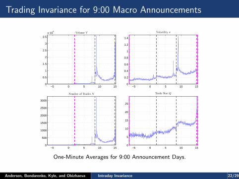
Trading Invariance for 9:00 Macro Announcements
−5 0 5 10 150
0.5
1
1.5
2
2.5
3
3.5x 10
4Volume V
−5 0 5 10 150
0.2
0.4
0.6
0.8
1
1.2
1.4
Volatility σ
−5 0 5 10 150
500
1000
1500
2000
2500
3000
Number of Trades N
−5 0 5 10 150
5
10
15
20
25
Trade Size Q
One-Minute Averages for 9:00 Announcement Days.
Andersen, Bondarenko, Kyle, and Obizhaeva Intraday Invariance 22/29

Trading Invariance for 9:00 Macro Announcements
8 10 12 14 16 181
2
3
4
5
6
7
8
9
logN vs logW , 9:00, All Days
8 10 12 14 16 181
2
3
4
5
6
7
8
9
logN vs logW , 9:00, Announcement Days
logNt vs. lnWt for 3 Minutes Before 9:00 (Dots), After 9:00 (Crosses).
Left: All Days; Right: 9:00 Announcements. Solid Line is prior OLS Fit.
Andersen, Bondarenko, Kyle, and Obizhaeva Intraday Invariance 23/29
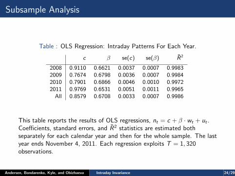
Subsample Analysis
Table : OLS Regression: Intraday Patterns For Each Year.
c β se(c) se(β) R2
2008 0.9110 0.6621 0.0037 0.0007 0.99832009 0.7674 0.6798 0.0036 0.0007 0.99842010 0.7901 0.6866 0.0046 0.0010 0.99722011 0.9769 0.6531 0.0051 0.0011 0.9965
All 0.8579 0.6708 0.0033 0.0007 0.9986
This table reports the results of OLS regressions, nt = c + β · wt + ut .Coefficients, standard errors, and R2 statistics are estimated bothseparately for each calendar year and then for the whole sample. The lastyear ends November 4, 2011. Each regression exploits T = 1, 320observations.
Andersen, Bondarenko, Kyle, and Obizhaeva Intraday Invariance 24/29
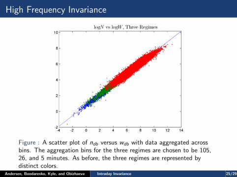
High Frequency Invariance
Figure : A scatter plot of ndb versus wdb with data aggregated acrossbins. The aggregation bins for the three regimes are chosen to be 105,26, and 5 minutes. As before, the three regimes are represented bydistinct colors.
Andersen, Bondarenko, Kyle, and Obizhaeva Intraday Invariance 25/29
High Frequency Invariance
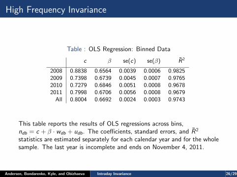
Table : OLS Regression: Binned Data
c β se(c) se(β) R2
2008 0.8838 0.6564 0.0039 0.0006 0.98252009 0.7398 0.6739 0.0045 0.0007 0.97652010 0.7279 0.6846 0.0051 0.0008 0.96782011 0.7998 0.6706 0.0056 0.0008 0.9679
All 0.8004 0.6692 0.0024 0.0003 0.9743
This table reports the results of OLS regressions across bins,ndb = c + β · wdb + udb. The coefficients, standard errors, and R2
statistics are estimated separately for each calendar year and for the wholesample. The last year is incomplete and ends on November 4, 2011.
Andersen, Bondarenko, Kyle, and Obizhaeva Intraday Invariance 26/29
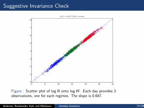
Suggestive Invariance Check
6 8 10 12 14 16 180
1
2
3
4
5
6
7
8
logN vs logW , Daily averages
Figure : Scatter plot of logN onto logW . Each day provides 3observations, one for each regimes. The slope is 0.687.
Andersen, Bondarenko, Kyle, and Obizhaeva Intraday Invariance 27/29
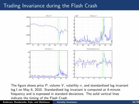
Trading Invariance during the Flash Crash
9 10 11 12 13 14 15−4
−3
−2
−1
0
1
2
3
4Standardized log I
9 10 11 12 13 14 151050
1100
1150
1200Price P
9 10 11 12 13 14 150
1
2
3
4
5
6
7
x 104
Volume V
9 10 11 12 13 14 150
2
4
6
8
10
Volatility σ
The figure shows price P, volume V , volatility σ, and standardized log invariantlog I on May 6, 2010. Standardized log invariant is computed at 4-minutefrequency and is expressed in standard deviations. The solid vertical linesindicate the timing of the Flash Crash.
Andersen, Bondarenko, Kyle, and Obizhaeva Intraday Invariance 28/29
Conclusions
Intraday Trading Activity Patterns Intimately Related
Traditional Theories: Transactions or Volume Govern Volatility
Invariance (Kyle & Obizhaeva) Motivates Alternative Intraday Relation
Critically, Trade Size Drops in specific Proportion with Volatility
For E-Mini, Tendency Observed by Andersen & Bondarenko RF, VPIN
Qualitative Prediction verified for Diurnal Pattern
Qualitative Prediction verified for Daily Regimes (Time Series)
Theoretical Justification for Invariance in this Context Loom Large
How will Findings Generalize across Market Structures?
Andersen, Bondarenko, Kyle, and Obizhaeva Intraday Invariance 29/29