Intraday Return Predictability, Informed Limit Orders, and

Algorithmic Trading

Darya Yuferova∗

October 2017

Abstract

I study the strategic choice of informed traders for market vs. limit orders by analyzingthe informational content of the limit order book. In particular, I examine intradayreturn predictability from market and limit orders for all NYSE stocks over 2002-2010, distinguishing between two sources of predictability: inventory management andinformation. In contrast to the traditional view in the literature, I find that informedlimit (not market) orders are the dominant source of intraday return predictability. Thefindings further indicate that the advent of algorithmic trading is associated with moreinformed trading, especially through market orders. Overall, my evidence emphasizesthe role of limit orders in informed trading, which has implications for theory, investors,and widely used measures of informed trading.

∗Norwegian School of Economics (NHH); e-mail address: darya.yuferova@nhh.no. I am grateful to DionBongaerts, Mathijs Cosemans, Sarah Draus, Thierry Foucault, Wenqian Huang, Lingtian Kong, AlbertMenkveld, Marco Pagano, Christine Parlour, Loriana Pelizzon, Dominik Rösch, Stephen Rush, Asani Sarkar,Elvira Sojli, Mark Van Achter, Mathijs van Dijk, Wolf Wagner, Jun Uno, Marius Zoican, participants of theNFN 2016 Young Scholars Finance Workshop, participants of the FMA 2015 Doctoral Consortium, partici-pants of the PhD course on “Market Liquidity” in Brussels, and seminar participants at Goethe University,Norwegian School of Economics, Norwegian Business School, Paris Dauphine University, Erasmus University,NYU Stern, and Tinbergen Insitute for helpful comments. I gratefully acknowledge financial support fromthe Vereniging Trustfonds Erasmus Universiteit Rotterdam. I am also grateful to NYU Stern and RotterdamSchool of Management, Erasmus University, where some work on this paper was carried out during my PhDstudies. This work was carried out on the National e-infrastructure with the support of SURF Foundation.I thank OneMarket Data for the use of their OneTick software.

1. Introduction

The limit order book is the dominant market design in equity exchanges around the

world.1 The prevalence of limit order book markets calls for a detailed understanding of

how such markets function. In particular, understanding the price discovery process on

these markets required a detailed study of the trader’s choice between submissions of market

and limit orders. The conventional wisdom in the microstructure literature used to be that

informed traders use only market orders, while uninformed traders use both market and

limit orders (for theoretical work see Glosten and Milgrom, 1985; Kyle, 1985; Glosten, 1994;

Seppi, 1997). Only recent studies explicitly consider the choice of informed traders for market

or limit orders.2 Informed traders can submit a market order and experience immediate

execution at the expense of the bid-ask spread (consume liquidity). Alternatively, informed

traders can submit a limit order and thus bear the risk of non-execution, as well as the risk

of being picked-off, but earn the bid-ask spread (provide liquidity).

The importance of the informed trader’s choice between market and limit orders is em-

phasized by a heated public debate about whether one group of market participants poses

negative externalities to another group of market participants due to informational asym-

metries. This informational advantage is especially pronounced for traders with superior

technologies for the collection and processing of information. Another feature that enhances

informational inequality in the market is the ability to continuously monitor and respond to

market conditions. Both characteristics are distinct characteristics of high-frequency traders

1According to Swan and Westerholm (2006), 48% of the largest equity markets are organized as pure limitorder book markets (e.g., Australian Stock Exchange, Toronto Stock Exchange, Tokyo Stock Exchange), 39%are organized as limit order books with designated market makers (e.g., New York Stock Exchange, BorsaItaliana), and the remaining 12% are organized as hybrid dealer markets (e.g., NASDAQ, Sao Paulo StockExchange) as of the beginning of 2000.

2For theoretical studies on the choice of uninformed traders between market and limit orders, see Cohen,Maier, Schwartz, andWhitcomb (1981), Chakravarty and Holden (1995), Handa and Schwartz (1996), Parlour(1998), Foucault (1999), Foucault, Kadan, and Kandel (2005), Goettler, Parlour, and Rajan (2005), and Roşu(2009); for theoretical studies on the choice of informed traders between market and limit orders see, Liuand Kaniel (2006), Goettler, Parlour, and Rajan (2009), and Roşu (2015); for empirical studies on the choicebetween market and limit orders on equity markets see, Bae, Jang, and Park (2003), Anand, Chakravarty, andMartell (2005), Bloomfield, O’Hara, and Saar (2005), and Baruch, Panayides, and Venkataraman (2015); forempirical studies on the choice between market and limit orders on foreign exchange markets see, Menkhoff,Osler, and Schmeling (2010), Kozhan and Salmon (2012), and Kozhan, Moore, and Payne (2014).

1

(a subset of algorithmic traders). Consistently, several papers identify algorithmic traders’

strategies that are disadvantageous for retail investors.3 Previous research has focused on

informed algorithmic trading via market orders with only one exception.4 In sum, under-

standing how informed trading takes place and what role algorithmic traders play in this

process are important questions to explore in modern market microstructure.

In this paper, I address these questions by studying intraday return predictability. Nat-

urally, orders submitted by informed traders contain information about future price move-

ments. If an informed trader actively uses market orders, an imbalance between buyer- and

seller-initiated volume may be informative about future price movements. If an informed

trader actively uses limit orders, the limit order book may contain information that is not

yet incorporated into the price. Therefore, strategies employed by informed traders may

induce intraday return predictability from market and limit order flows alike.

My main contribution to the literature is twofold. First, I contribute to the literature

on intraday return predictability. I distinguish between two sources of intraday return pre-

dictability (inventory management and private information). My findings indicate that the

main source of the intraday return predictability is private information embedded in limit

orders. Furthermore, I show that this result holds for a wide cross-section of stocks and

through a prolonged time period.5 Second, my paper contributes to the ongoing debate

on the role of algorithmic traders (especially it subset, high-frequency traders) in informed

trading activity (see Biais and Foucault (2014) for review on high-frequency trading activity

and market quality). My evidence suggests that an increased degree of algorithmic trading

activity leads to an increased usage of both informed limit and informed market orders (with

3See for theoretical work, e.g., Foucault, Hombert, and Roşu, 2015; Biais, Foucault, and Moinas, 2015;Foucault, Kozhan, and Tham, 2015; Jovanovic and Menkveld, 2015; see for empirical work, e.g., McInishand Upson, 2012; Hirschey, 2013; Brogaard, Hendershott, and Riordan, 2014; Foucault, Kozhan, and Tham,2015.

4Brogaard, Hendershott, and Riordan (2015) examine informed trading via both market and limit ordersby high-frequency traders for the sample of 15 Canadian stocks from October 2012 to June 2013.

5For papers studying intraday return predictability from the limit order book in equity markets see Irvine,Benston, and Kandel (2000), Kavajecz and Odders-White (2004), Harris and Panchapagesan (2005), Cao,Hansch, and Wang (2009), Cont, Kukanov, and Stoikov (2013), and Cenesizoglu, Dionne, and Zhou (2014).However, none of these papers uses such comprehensive data as used in this paper.

2

the main effect concentrated in market orders). Informed limit orders still remain the main

source of the intraday return predictability even after increased degree of algorithmic trading

activity.

The analysis is organized in two stages. First, I analyze intraday return predictability

from market and limit order flows and separate the effect of informed trading from the effect

of inventory management. Second, I analyze the impact of algorithmic trading on the choice

between market and limit orders made by an informed trader. In particular, I exploit a

quasi-natural experiment to establish a causal inference between algorithmic trading and

intraday return predictability from market and limit order flows. I also test recent theories of

the choice between informed trading through market versus limit orders by exploiting their

predictions regarding differences between low and high volatility stocks.

Using tick-by-tick trade data and data on the first 10 best levels of the consolidated

limit order book for the NYSE from the Thomson Reuters Tick History (TRTH) database, I

construct a time series of mid-quote returns, market order imbalance, and snapshots of the

first 10 best levels of the U.S. consolidated limit order book at the one-minute frequency at

the individual stock level. The sample covers all NYSE-listed common stocks for the years

2002-2010. TRTH data used in this paper are very comprehensive. In particular, for the

stocks under consideration, I have information for 1.36 billion trades and 8.54 billion limit

order book updates.

Intraday return predictability from limit order book data can arise from two sources.

First, inventory management (Hypothesis 1) may induce intraday return predictability by

generating price pressure as a result of limited risk-bearing capacity of risk-averse liquidity

providers (e.g., Stoll, 1978; Menkveld, 2013; Hendershott and Menkveld, 2014). Second,

private information (Hypothesis 2) may also induce intraday return predictability (see Liu

and Kaniel, 2006; Goettler, Parlour, and Rajan, 2009; Roşu, 2015). The latter source of

return predictability is the main focus of this paper. I approach the problem of isolating

private information source of intraday return predictability from two angles. First, inventory

management should result in temporary price effects, while private information should result

3

in permanent price effects. Therefore, controlling for lagged returns in predictive regressions

allows me to separate inventory management effects from the effects of private information.

Second, I run a VAR model and decompose market and limit order flows into two compo-

nents: inventory-related (fitted values) and information-related (surprises) components. The

use of surprises as a proxy for informed market and limit order flows is motivated by the fact

that both limit and market order flows are persistent (e.g., Hasbrouck, 1991; Biais, Hillion,

and Spatt, 1995; Ellul, Holden, Jain, and Jennings, 2003; Chordia, Roll, and Subrahmanyam,

2005) and that this persistence is attributable to reasons other than information (e.g., De-

gryse, de Jong, and van Kervel, 2013). Huang and Stoll (1997), Madhavan, Richardson, and

Roomans (1997), and Sadka (2006) also use surprises in market order imbalance to isolate

the adverse selection component of the bid-ask spread.

Combining these two approaches, I run the predictive regressions with lagged surprises

in returns, lagged surprises in market order imbalance, and lagged surprises in depth con-

centration at the inner and outer levels of the ask and bid sides of the limit order book.

In this specification any remaining inventory management effects should be captured by the

coefficient of lagged surprises in returns. I use both market order flow and limit order book

variables in the predictive regressions to capture the trader’s choice between market and

limit orders. Inclusion of market order imbalance is also motivated by Chordia, Roll, and

Subrahmanyam (2005, 2008), who show that market order imbalance is predictive of future

price movements.

The findings of the first part of the analysis indicate that the main source of intraday

return predictability is private information (inventory management (lagged returns) accounts

only for 30% of total predictive power as measured by the average incremental adjusted R2

from the predictive regressions). In addition, the results indicate that informed trading

through the limit order book accounts for 50% of return predictability that is 30% greater

than a fraction of return predictability induced by informed trading through market orders.

The findings contradict the traditional view that only market orders are used for informed

trading. Furthermore, the findings suggest that informed trading via market orders is of less

4

importance than informed trading via limit orders.

In the second part of the analysis, I investigate how the presence of algorithmic traders

affects the order choices made by informed traders. This is a non-trivial task as algorithmic

traders endogenously determine the extent of their participation in each stock at each point

in time. I follow the approach of Hendershott, Jones, and Menkveld (2011) and use the NYSE

Hybrid Market introduction — a permanent technological change in market design6 — as

an instrumental variable to help determine the causal effects of algorithmic trading activity

on intraday return predictability from informed market and limit order flows. The rollout

to the Hybrid Market was implemented in a staggered way, which helps clean identification.

I follow Hendershott, Jones, and Menkveld (2011) and Boehmer, Fong, and Wu (2015) and

use the daily number of best bid-offer quote updates relative to the daily trading volume (in

$10,000) as a proxy for algorithmic trading activity on each stock-day.

I develop two competing hypotheses of the effects of algorithmic trading on informed

traders’ choices: the efficient technology hypothesis (Hypothesis 3) and the competition

hypothesis (Hypothesis 4). On the one hand, the technological advantage of algorithmic

traders makes limit orders more attractive to them as they are able to reduce pick-off risks

better than the other market participants (the efficient technology hypothesis). On the

other hand, competition between algorithmic traders for (trading on) the same information

makes market orders more attractive to them as they guarantee immediate execution (the

competition hypothesis).

The results show that algorithmic trading activity leads to increased informational content

in both market and limit orders. However, an increase in the predictive power associated with

limit order book variables (the efficient technology hypothesis) is smaller than the increase

in predictive power associated with market order imbalance (the competition hypothesis).

Although the evidence is consistent with both hypotheses, the effects of the competition

hypothesis seem to dominate the effects of the efficient technology hypothesis. In other

6NYSE Hybrid Market introduction allowed market orders to “walk” through the limit order book auto-matically and thus, increased automation and speed (Hendershott and Moulton, 2011).

5

words, increased algorithmic trading activity is associated with a relative shift from liquidity

provision (limit orders) to liquidity consumption (market orders) by informed traders.

Overall, my paper provides evidence that informed traders tend to act more often as

liquidity providers (use limit orders), than liquidity demanders (use market orders). However,

with an increased presence of algorithmic traders, the amount of informed liquidity provision

increases less than the amount of informed liquidity consumption. One important implication

of my analysis concerns measures of asymmetric information and/or informed trading (e.g.,

PIN measure by Easley, Kiefer, O’Hara, and Paperman (1996); adverse selection component

of bid-ask spread by Glosten and Harris (1988) and Huang and Stoll (1997)), which have

been used widely in studies on market microstructure, asset pricing, and corporate finance.7

These measures are exclusively based on market orders, and thus neglect the lion’s share of

informed trading on the equity markets — informed trading via limit orders.

2. Hypotheses

In this section, I develop the hypotheses for the tests of the choice between limit and mar-

ket orders by informed traders based on the evidence from intraday return predictability. In

section 2.1, I develop two hypotheses regarding the sources of intraday return predictability:

the inventory management hypothesis and the private information hypothesis. In section 2.2,

I describe the hypotheses regarding the effect of algorithmic trading activity on the strate-

gies employed by informed traders (the efficient technology hypothesis and the competition

hypothesis). The effect of the realized volatility is described in section 2.3.

2.1. Sources of intraday return predictability

Intraday return predictability from the limit order book can arise from two (not mutu-

ally exclusive) sources: inventory management and private information. Under the inventory

management hypothesis, depth concentration at the inner levels of the limit order book indi-

cates that a liquidity provider wants to unload inventory. This situation creates a temporary

7E.g., Easley, Hvidkjaer, and O’Hara (2002), Vega (2006), Chen, Goldstein, and Jiang (2007), Korajczykand Sadka (2008), Bharath, Pasquariello, and Wu (2009), and Easley, de Prado, and O’Hara (2012).

6

price impact that is reverted as soon as the inventory position of the liquidity provider is

liquidated (e.g., Stoll, 1978; Ho and Stoll, 1981; Menkveld, 2013; Hendershott and Menkveld,

2014). Indeed, a liquidity provider will be hesitant to immediately replenish the ask side of

the limit order book as a large market buy order walks through the limit order book, because

she would prefer to liquidate excessive inventory first. It is optimal for her to post aggressive

limit orders on the bid side of the book, while on the ask side she will post a limit order

deep in the limit order book. In this way, she encourages other market participants to sell

her their stocks while discouraging them from buying from her. Therefore, I formulate the

inventory management hypothesis as follows:

H1 (the inventory management hypothesis): Depth concentration at the inner levels of the

ask (bid) sides of the limit order book is associated with decrease (increase) in future stock

returns, with depth concentration at the outer levels having virtually no effect on future stock

returns.

Under the traditional approach to the adverse selection problem in equity markets only

inventory management should drive intraday return predictability from the limit order book.

This approach is built under the assumption of informed traders only using market orders

(e.g., Glosten and Milgrom, 1985; Kyle, 1985; Glosten, 1994; Seppi, 1997), which may be

an inadequate approximation of reality. Later studies build upon this initial work and allow

both informed and uninformed traders to choose between the order types (Liu and Kaniel,

2006; Goettler, Parlour, and Rajan, 2009; Roşu, 2015).

Based on theoretical predictions from Goettler, Parlour, and Rajan (2009), an informed

trader, who receives good news about a stock, has three different options to exploit this

information. First, the trader can submit a buy market order. Second, the trader can submit

a limit buy order at the inner level of the bid side of the limit order book; this limits execution

probability, but saves transaction costs. Third, the trader can also submit a limit sell order

at the outer levels of the ask side of the limit order book in combination with one of the two

above mentioned orders to lock-in the benefit from the price difference. The opposite is true

for the bad news scenario.

7

In reality, an informed trader’s choice between market and limit orders depends on the

strength of the signal received, the lifespan of the information, the ratio of informed to

uninformed traders, etc. In the case of a weak and very short-lived signal, the trader is likely

to use market orders. In the case of very strong signal that has a relatively long lifespan, the

trader is likely to use limit orders at the inner and outer levels of the limit order book. In

the case of the average signal with a short lifespan (which I believe is the dominant type of

signal), the trader is likely to use a mixture of market and limit orders (see Table 1).

Therefore, I formulate the private information hypothesis as follows:

H2 (the private information hypothesis): Depth concentration at the inner levels of the

ask side of the limit order book is associated with decrease in future stock returns, while depth

concentration at the outer levels of the ask side of the limit order book is associated with

increase in future stock returns. The opposite is true for the bid side of the limit order book.

The main purpose of this paper is to test the private information hypothesis and inves-

tigate the effect of algorithmic traders on the informed trader’s choice between market and

limit orders discussed in the next subsection.

2.2. Effect of algorithmic trading activity

During the past decade, a new group of market participants — algorithmic traders — has

emerged and evolved into a dominant player responsible for the majority of trading volume.

Algorithmic trading “is thought to be responsible for as much as 73 percent of trading volume

in the United States in 2009” (Hendershott, Jones, and Menkveld, 2011, p. 1). Therefore,

it is a natural question to ask what role algorithmic traders are playing in informed trading

process and to what extent their presence affects the informed trader’s choice between market

and limit orders.

Possessing private information is equivalent to having capacity to absorb and analyze pub-

licly available information (including information from the past order flow) faster than other

market participants (Foucault, Hombert, and Roşu, 2015; Foucault, Kozhan, and Tham,

2015; Menkveld and Zoican, 2015). Efficient information processing technology is a distinct

feature of algorithmic traders, hence they are more likely to be informed than other market

8

participants. However, ex ante it is not clear whether algorithmic traders would prefer to use

market or limit orders to profit from their informational advantage.

On the one hand, limit orders are attractive for traders who can accurately predict execu-

tion probabilities, continuously monitor the market, and quickly adapt to market conditions.

Algorithmic traders possess all of these characteristics. Thus, they may be inclined to use

limit orders for informed trading.

On the other hand, competition among informed traders will lead to a faster price discov-

ery and a shorter lifespan for the information obtained by the informed trader. Algorithmic

traders compete for the same information by processing the same news releases or by ana-

lyzing past order flow patterns as fast as possible. In a competitive market, a trader must

be the first in line to trade on information in order to profit from it. Given that only market

orders can guarantee immediate execution, algorithmic traders may be inclined to use mar-

ket orders for informed trading. Therefore, I formulate two competing hypotheses for the

strategies employed by informed algorithmic traders:

H3 (the efficient technology hypothesis): The predictive power of informed market orders

is lower for stocks subject to high algorithmic trading activity than for stocks subject to low

algorithmic trading activity. On the other hand, the predictive power of informed limit orders

is higher for stocks subject to high algorithmic trading activity than for stocks subject to low

algorithmic trading activity.

H4 (the competition hypothesis): The predictive power of informed market orders is higher

for stocks subject to high algorithmic trading activity than for stocks subject to low algorithmic

trading activity. On the other hand, the predictive power of informed limit orders is lower for

stocks subject to high algorithmic trading activity than for stocks subject to low algorithmic

trading activity.

2.3. Effect of realized volatility

According to Goettler, Parlour, and Rajan (2009), informed traders may prefer market

orders to limit orders at the inner levels of the limit order book for high volatility stocks and

limit orders at the inner levels of the limit order book to market orders for low volatility stocks.

9

The intuition is as follows. Posting a limit order is like writing an option (e.g., Copeland and

Galai, 1983; Jarnecic and McInish, 1997; Harris and Panchapagesan, 2005). It is known that

the sensitivity of the option price to the changes in the volatility of the underlying asset, i.e.,

vega (ν), is positive. In other words, the option price increases when the volatility of the

underlying asset increases. In this way, the option writer gets compensated for the increased

risk of option execution. Thus, the increased volatility of the stock will make limit orders

riskier and hence, less profitable. In addition, market orders become more profitable due

to picking off the stale limit orders posted by slow (and most likely uninformed) traders.

And last but not least, in a highly volatile environment it is harder to distinguish between

informed and uninformed market orders and hence, hiding informed trading is easier.

Given that on an intraday horizon, realized volatility based on the mid-quote returns is a

good proxy for fundamental volatility, I formulate the realized volatility hypothesis as follows:

H5 (the realized volatility hypothesis): The predictive power of informed market orders is

greater for high volatility stocks than for low volatility stocks. On the other hand,the predictive

power of informed limit orders concentrated at the inner levels of the limit order book is greater

for low volatility stocks than for high volatility stocks.

3. Data, Variables, and Summary Statistics

In this section, I describe the data, variables, and summary statistics. I obtain intraday

consolidated data on trades and the 10 best levels of the limit order book for the U.S. market

from the Thomson Reuters Tick History (TRTH) database. The TRTH database is provided

by the Securities Industry Research Centre of Asia-Pacific (SIRCA). Data on trades and best

bid-offer quotes are available since 1996. Data on the limit order book levels are available

only from 2002 as the NYSE opened its limit order book to the public on January 24, 2002.

The limit order book data provided by TRTH does not include order level information (e.g.,

no order submission, revision, or cancellation details), only the 10 best price levels and the

depth on bid and ask sides of the book that is visible to the public. The data comes from the

consolidated tape. In other words, the best bid-offer reported in the data is the best bid-offer

10

for any exchange in the U.S. The same applies to the other levels of the limit order book.

TRTH data are organized by Reuters Instrumental Codes (RICs), which are identical to

TICKERs provided by the Center for Research in Security Prices (CRSP). Merging data

from CRSP and TRTH allows me to identify common shares that indicate the NYSE as

their primary exchange and to use company specific-information (e.g., market capitalization,

turnover, etc.). This study is limited to NYSE-listed stocks only as intraday return pre-

dictability from limit order book information as well as the behavior of the informed traders

could be very sensitive to market design. Hence, it seems inappropriate to put, for example,

the NASDAQ (hybrid dealer market) and NYSE (limit order book with designated market

makers) data together.

The available data for the limit order book cover the period from 2002 to 2010. The

joint size of the trade and limit order book data reaches 2.5 terabytes. In order to make the

analysis feasible, I compute one-minute mid-quote returns and market order imbalances, and

take snapshots of the limit order book at the end of each one-minute interval. I filter the

data to discard faulty data entries and data entries outside continuous trading session (see

the Appendix for details).

3.1. Variable descriptions

In this section, I describe the variables used to study the choice of informed traders

between market and limit orders by means of intraday return predictability from the limit

order book. In particular, I look at the return predictability one-minute ahead. Therefore, I

need intraday data on returns, market order imbalances (MOIB), and limit order book data

(LOB) at one-minute frequency. For all the variables, I discard overnight observations.

I follow Chordia, Roll, and Subrahmanyam (2008) and compute one-minute log-returns

(Ret) based on the prevailing mid-quotes (average of the bid and ask prices) at the end of

the one-minute interval, rather than the transaction prices or mid-quotes matched with the

last transaction price. In this way I avoid the bid-ask bounce and ensure that the returns for

every stock are indeed computed over a one-minute interval. I implicitly assume that there

are no stale best bid-offer quotes in the sample, thus I consider a quote to be valid until a

11

new quote arrives or until a new trading day starts.

To calculate a one-minute MOIB, I match trades with quotes and sign trades using the

Lee and Ready (1991) algorithm. TRTH data are stamped to the millisecond, therefore the

Lee and Ready (1991) algorithm is quite accurate. In particular, a trade is considered to be

buyer-initiated (seller-initiated) if it is closer to the ask price (bid price) of the prevailing

quote. For each one-minute interval, I aggregate the trading volume in USD for buyer- and

seller-initiated trades separately at the stock level. Thereafter, I subtract seller-initiated

dollar volume from buyer-initiated dollar volume to obtain MOIB.

There are multiple ways to describe the limit order book. Most of the papers that study

intraday return predictability either focus on different levels of the limit order book or on the

corresponding ratios of these levels between the ask and bid sides of the limit order book.

For instance, Wuyts (2008), Cao, Hansch, and Wang (2009), and Cenesizoglu, Dionne, and

Zhou (2014) use slopes and depth at different levels of the limit order book to summarize

its shape. However, due to variation in the shape of the limit order book as well as in the

number of available levels of the limit order book (in my sample the daily average number

of levels can be as low as just six levels), I believe that definition of inner and outer levels

by means of a relative threshold is more suitable than definition by means of the number of

levels in the limit order book (e.g., levels from 2 to 5 are inner levels and levels from 6 to 10

are outer levels).

Examples of a relative approach to limit order book description are Cao, Hansch, and

Wang (2009), who also use volume-weighted average price for different order sizes to describe

the limit order book, and Kavajecz and Odders-White (2004), who use a so-called “near-

depth” measure, which is a proportion of the depth close to the best bid-offer level relative

to the cumulative depth within a certain price range.

For the purpose of testing the private information hypothesis, I focus on the ratios within

the ask and bid sides separately, rather than across the ask and bid sides of the limit order

book. I use a modification of the “near-depth” measure introduced by Kavajecz and Odders-

White (2004). First, I compute a snapshot of the ask and bid sides of the limit order book

12

at the end of each one-minute interval. Then, I define the inner depth concentration as

cumulative depth lying between the mid-quote and one-third of the total distance between

the 10th available limit price and the mid-quote relative to the total cumulative depth of the

ask and bid side of the limit order book separately (Ask Inner and Bid Inner). I define the

outer depth concentration as cumulative depth lying between one-third and two-thirds of the

total distance between the 10th available limit price and the mid-quote relative to the total

cumulative depth of the ask and bid side of the limit order book separately (Ask Outer and

Bid Outer). Please refer to Table 2 for the summary of variables’ descriptions.

My relative approach allows me to define inner and outer levels of the limit order book

even if not all 10 levels are present for a particular stock at a particular time. Hence, I can

define in unified fashion the levels that are close to the best bid-offer level, as well as the

levels that are far away from the best bid-offer level across stocks and through time.

3.2. Summary statistics

Table 3 presents summary statistics for the one-minute mid-quote returns (Ret), dollar

market order imbalance (MOIB), and depth concentration at the inner levels (Bid Inner

and Ask Inner) and outer levels (Bid Outer and Ask Outer) of the ask and bid sides of

the limit order book (LOB), and cutoff points between the inner and outer levels of the

limit order book measured relative to the mid-quote (Bid Cutoff and Ask Cutoff) at the

end of each one-minute interval for the whole period (from January 2002 to December 2010)

and two sub-periods (from January 2002 to June 2006 and from July 2006 to December

2010). I start with winsorizing all variables at the 1% and 99% levels on a stock-day basis.

Then, I compute averages of the one-minute observations for mid-quote returns (Ret), dollar

market order imbalance (MOIB), and depth concentration at the inner and outer levels of

the ask and bid sides of the limit order book per stock-day. Afterwards, I winsorize stock-

day averages of the variables at the 1% and 99% levels based on the whole sample period or

sub-periods and compute summary statistics.

The mean of the daily average one-minute mid-quote returns is -0.003 basis points for

the whole sample period (see Panel A of Table 3). The average negative return is due to the

13

inclusion of the recent financial crisis period in the sample. Indeed, in the first half of the

sample period the average returns are 0.014 basis points, while in the second half of the period

the average returns are -0.02 basis points. The mean of the daily average one-minute dollar

market order imbalance is $4,133.34. This indicates that on average there is more buying

than selling pressure in the market. However, this buying pressure is much more moderate

at $840.15 – when I focus on the second half of the sample period due to the inclusion of the

recent financial crisis.

Panel A of Table 3 also shows the depth concentration at the inner and outer levels

separately of the ask and bid side of the limit order book for the whole sample period. The

average proportion of the cumulative depth at the inner levels of the limit order book is

31.49% and 32.19% of the ask and bid side of the limit order book, respectively. The average

proportion of the cumulative depth at the outer levels of the limit order book is 31.36%

and 31.20% of the ask and bid sides of the limit order book, respectively. Although the

average depth concentration is very similar for the inner and outer levels for both ask and

bid sides of the limit order book, depth concentration at the inner levels exhibits higher

variation than depth concentration at the outer levels both in terms of within and between

standard deviations. Notably, the ask and bid sides of the limit order book exhibit similar

characteristics in terms of the depth concentration at the inner and outer levels.

Panel A of Table 3 also reports the cutoff points between inner and outer levels of the ask

and bid sides of the limit order book measured as a percentage deviation from the mid-quote.

For the whole sample period, the cutoff point (one-third of the total distance between the

10th available limit price and the mid-quote) is 1.47% and -1.43% of the ask and bid sides

of the limit order book, respectively.

Sub-period analysis (see Panels B and C of Table 3) reveals that although on average

through the whole sample period depth concentration at the inner and outer levels for both

sides of the limit order book is similar, depth concentration at the inner levels tends to de-

crease over time, while depth concentration at the outer levels tends to increase over time.

14

In particular, in the first half of the sample period, depth concentration at the inner levels

of the ask (bid) side of the limit order book is 42.66% (45.31%). In the second half of the

sample period, depth concentration at the inner levels of the ask (bid) side of the limit order

book is 21.53% (20.47%). In the first half of the sample period, depth concentration at the

outer levels of the limit order book of the ask (bid) side of the limit order book is 25.49%

(24.69%), while in the second half of the sample period it reaches 36.59% (37.03%).

This trend in the limit order book composition is also reflected in the cutoff points between

the inner and outer levels of the limit order book. In particular, in the first half of the sample

period, price levels of the limit order book are more dispersed than in the second half of the

sample period. Hence, for the first half of the sample period I define inner depth as depth

concentrated at price levels that do not differ from the mid-quote more than 2.34% (2.45%) of

the ask (bid) side of the limit order book, respectively. The cutoff points for the second half

of the period are 0.68% (0.51%) for the ask (bid) side of the limit order book, respectively.

This decreasing (increasing) trend in depth concentration at the inner (outer) levels of

the limit order book can be also observed in Panel A of Figure 1. Panel B of Figure 1 shows

the trend in cutoff points between the inner and outer levels of the limit order book.

The composition changes in the limit order book may be attributable to the different

structural changes of the NYSE during the sample period such as autoquote introduction

in 2003 (Hendershott, Jones, and Menkveld, 2011), NYSE Hybrid introduction in 2006-2007

(Hendershott and Moulton, 2011), Reg NMS implementation in 2007, and replacement of

the specialist by designated market makers at the end of 2008.

4. Methodology

In this section, I describe the methodology used in the paper in order to investigate

whether market and/or limit orders are used for informed trading. In particular, I empirically

distinguish between two sources of intraday return predictability: inventory management

(Hypothesis 1) and private information (Hypothesis 2). Given that the main goal of this

paper is to investigate the informed trader’s choice between market and limit orders, the

15

latter source of the intraday return predictability is the one I focus on.

I run stock-day predictive regressions at one-minute frequency using one-minute mid-

quote returns as the dependent variable. As explanatory variables I use lagged returns, lagged

market order imbalance (MOIB), and lagged depth concentration at the inner and outer

levels of the ask and bid sides of the limit order book. I includeMOIB in the model as I want

to show that the LOB variables contain useful information for intraday return predictability

beyond MOIB. Controlling for lagged returns allows me to differentiate between temporary

effect (inventory management) and permanent effect (private information). The regression

equation is given by:

Rett = α + β1Rett−1 + β2MOIBt−1 + β3Bid Innert−1 + β4Ask Innert−1+ (1)

+β5Bid Outert−1 + β6Ask Outert−1 + εt

where Rett is the mid-quote return during the t-th one-minute interval,MOIBt−1 is the dollar

market order imbalance during the (t − 1)-th one-minute interval, LOBt−1: Bid Innert−1,

Ask Innert−1, Bid Outert−1, Ask Outert−1 are the depth concentrations at the inner and

outer levels of the ask and bid sides of the limit order book at the end of the (t − 1)-th

one-minute interval.

As a next step, I identify the private information component of the market and limit

order flows and enhance the above mentioned methodology. Hasbrouck (1991) and Chordia,

Roll, and Subrahmanyam (2005) show that MOIB is positively autocorrelated. Moreover,

Biais, Hillion, and Spatt (1995) and Ellul, Holden, Jain, and Jennings (2003) show that

order flow is also persistent for limit orders. Biais, Hillion, and Spatt (1995) argue that

there are three possible reasons for the order flow persistence: order splitting, imitation of

other traders’ behavior, and reaction to the public information in a sequential manner (e.g.,

due to the differences in trading speed). Degryse, de Jong, and van Kervel (2013) show

that order flow persistence is caused by reasons other than private information. Previous

empirical studies (e.g., Huang and Stoll, 1997; Madhavan, Richardson, and Roomans, 1997;

Sadka, 2006) use unexpected changes in the market order flow in order to isolate information-

16

related component. I extend this approach one step further and apply it to market and limit

order flows. I argue that it is an appropriate extension as both market and limit order flows

are persistent. Therefore, I use unexpected changes in the order flow for both market and

limit orders as a proxy for the private information component of the order flow.

I obtain the surprises in returns, MOIB, and LOB variables by estimating stock-day

V AR(k) regression (number of lags, k, can take values from 1 to 5 and is selected by AIC

criteria) and keeping the residual values:

Xt = α +l=k∑l=1

βXt−l + εt (2)

where Xt is a vector that includes Rett, MOIBt, Bid Innert, Ask Innert, Bid Outert, and

Ask Outert measured at the t-th one-minute interval; εt is vector of residuals that includes

the RetUt , MOIBUt , Bid InnerUt , Ask InnerUt , Bid OuterUt , and Ask OuterUt .

In the remainder of the paper, the superscript U indicates a residual value from V AR(k)

rather than the variable itself. Misspecification of the V AR(k) model may lead to some

inventory effects ending up in the surprises. In order to address this issue, I include lagged

surprises in returns as explanatory variable in the predictive regressions to capture return

reversal, which is a distinct feature of the inventory management hypothesis. I run predictive

regressions per stock-day with lagged surprises in returns, lagged surprises in MOIB, and

lagged surprises in depth concentration at the inner and outer levels of the ask and bid sides

of the limit order book as explanatory variables:

Rett = α + β1RetUt−1 + β2MOIBU

t−1 + β3Bid InnerUt−1 + β4Ask Inner

Ut−1+ (3)

+β5Bid OuterUt−1 + β6Ask Outer

Ut−1 + εt

5. Empirical Results

In this section, I provide empirical evidence for the informed trader’s choice between

market and limit orders by analyzing intraday return predictability from market and limit

order flows (section 5.1). Then, I discuss the role of algorithmic trading activity in the choice

17

made by informed trader (section 5.2). In section 5.3, I provide supplementary analysis of

the effects of realized volatility on the informed trader’s choice.

5.1. Intraday return predictability

I start with examining whether limit order book variables are useful in predicting intra-

day returns without explicitly decomposing order flow into inventory- and information-related

components. Table 4 presents estimation results of equation (1): predictive stock-day regres-

sions of one-minute mid-quote returns on one-minute lagged mid-quote returns, one-minute

lagged market order imbalance, and one-minute lagged depth concentration at the inner and

outer levels of the ask and bid sides of the limit order book.

Panel A of Table 4 reports average coefficients together with average Newey-West t-

statistics, as well as the proportion of the regressions that have significant individual t-

statistics.8 Rett−1 is negatively related to the future returns. Such return reversals are

in line with the inventory management hypothesis (Hypothesis 1). MOIBt−1 is positively

related to future stock returns (in line with, e.g., Chordia, Roll, and Subrahmanyam, 2005,

2008). In particular, theMOIBt−1 coefficient is 4.65 and is positive and significant in 26.43%

of the stock-day regressions. These results hold for the whole sample period as well as for

the sub-periods.9 The increase of one within standard deviation in MOIBt−1 is associated

with a 0.72 basis points increase in the future returns, which is equivalent to an increase of

1.24 within standard deviation for returns.

In line with the inventory management (Hypothesis 1) and informed limit orders (Hy-

pothesis 2) hypotheses, depth concentration at the inner levels of the bid (ask) sides of the

limit order book, Bid Innert−1 (Ask Innert−1) is positively (negatively) related to the fu-

ture price movements. For the whole sample period, one within standard deviation increase

8To compute average Newey-West t-statistics, I do the following steps (following Rösch, Subrahmanyam,and van Dijk, 2015). First, I use a time series of the estimated coefficients for each stock to compute Newey-West t-statistics (Newey and West, 1987). Second, I average the cross-section of the Newey-West t-statisticsto determine the average Newey-West t-statistics estimate.

9As a comparison, Rösch, Subrahmanyam, and van Dijk (2015) document that coefficient of MOIBt−1

is 3.79 and is positive and significant in 30.07% of the predictive regressions using only lagged dollar marketorder imbalance over 1996-2010 for NYSE common stocks.

18

in Bid Innert−1 (Ask Innert−1) corresponds to an increase of future returns by 0.35 basis

points (decrease of future returns by -0.35 basis points), which is equivalent to an increase

of 0.61 within standard deviation for returns (decrease of 0.61 within standard deviation for

returns).

However, the fact that Bid Outert−1 (Ask Outert−1) is negatively (positively) related to

future price movements in the second half of the period cannot be explained under the inven-

tory management hypothesis (Hypothesis 1), while it is true under the private information

hypothesis (Hypothesis 2). Notably, the sign of Bid Outert−1 (Ask Outert−1) changes from

insignificantly positive (negative) in the first half of the sample period to significantly negative

(positive) in the second half of the sample period. In other words, informational content at

the outer levels of the limit order book is lower in the first half of the sample period compared

to the second half of the sample period. These results are also in line with increasing depth

concentration at the outer levels of the limit order book and decreasing depth concentration

at the inner levels of the limit order book over the sample period. For the whole sample

period, one within standard deviation increase in Bid Outert−1 (Ask Outert−1) corresponds

to decrease of future returns by -0.017 basis points (increase of future returns by 0.012 basis

points), which is equivalent to decrease of 0.03 within standard deviation for returns (increase

of 0.02 within standard deviation for returns).

Remarkably, the effects of the ask and bid sides of the limit order book are similar in terms

of the absolute size of the coefficients. However, the median of daily correlation coefficients

between Bid Innert−1 and Ask Innert−1 (Bid Outert−1 and Ask Outert−1) is quite low –

at only 6.24% (2.21%). Put differently, the depth concentration of the ask and bid sides of

the limit order book tend to vary largely independently from each other, thus their effects

on future returns should not offset each other.

At the same time, Panel A of Table 4 shows a clear discrepancy in the absolute size of the

coefficients between depth concentration at the inner and outer levels: 1.89 (-2.02) to -0.16

(0.11) of the bid (ask) side during the whole sample period, respectively.10 This discrepancy

10A natural concern is that the inner and outer levels of the limit order book are negatively correlated by

19

could be due to the fact that outer levels are not likely to be used for inventory management.

In addition, outer levels are used for informed trading if and only if an informed trader

receives a relatively strong signal, which is unlikely to happen regularly on the market.

In order to measure the relative importance of market and limit order variables, I look

at the R2 decomposition of the predictive regressions. Panel B of Table 4 shows that the

average adjusted R2 of the predictive regressions is equal to 1.64% for the whole sample

period. Adjusted R2 attributable toMOIBt−1 is 0.34% in absolute terms, which accounts for

20.66% of the total explanatory power. As a comparison, Chordia, Roll, and Subrahmanyam

(2008) document an adjusted R2 of 0.51% for predictive regressions using only lagged dollar

market order imbalance for the 1993-2002 period, which is of the same order of magnitude

as my estimate. Lagged return accounts for 32.38% of the total predictive power, while

46.96% of the total predictive power comes from the limit order book variables (with 27.79%

attributable to the depth concentration at the inner levels of the limit order book and 19.17%

attributable to the depth concentration at the outer levels of the limit order book).

My results are also consistent with Cao, Hansch, and Wang (2009), who document an

increase in adjusted R2 after inclusion of additional levels of the limit order book with a

monotonic decrease of the added value for each additional level. My results are however

at odds with Cont, Kukanov, and Stoikov (2013), who argue that only imbalances at the

BBO level drive intraday return predictability. Despite the fact that Cao, Hansch, and Wang

(2009) and Cont, Kukanov, and Stoikov (2013) also investigate intraday return predictability

from the limit order book, the data used in their studies is quite limited. Specifically, Cao,

Hansch, and Wang (2009) use one month of data on 100 stocks traded on the Australian Stock

Exchange, while Cont, Kukanov, and Stoikov (2013) use one month of data on 50 stocks from

S&P 500 constituents. Overall, my results allow me to draw more generalizable conclusions

regarding intraday return predictability and observed time series and cross-sectional patterns.

construction. If there is an extremely high correlation between depth concentration at the inner and outerlevels of the limit order book, I can run into a multicollinearity problem. However, across all stock-days,these correlation coefficients never fall below -70%, and the median value is around -46% for both ask andbid sides of the limit order book.

20

The sub-period analysis yields the following results. Total predictive power of the re-

gressions decreases slightly from 1.71% in the first half of the sample period to 1.58% in the

second half. This decrease is attributable to the limit order book (adjusted R2 decreases

from 0.85% to 0.71%). The predictive power of the MOIB increases slightly from 0.33% to

0.35%. This evidence is consistent with the fact that intraday return predictability from the

limit order book is a persistent phenomenon during 2002-2010 for all NYSE-listed common

stocks.

Next, I enrich the analysis discussed above in order to emphasize the importance of private

information source of intraday return predictability. To determine the pure effect of private

information on intraday return predictability from market and limit order flows, I follow the

previous literature (e.g., Huang and Stoll, 1997; Madhavan, Richardson, and Roomans, 1997;

Sadka, 2006) and use surprises in market and limit order flows to define the informational

component of the order flows. I calculate surprises as residual values of the V AR(k) regression

on a stock-day basis with the number of lags determined by AIC criteria (see equation 2). I

then repeat the above-mentioned analysis with these surprises used as explanatory variables

(see equation 3). I use superscript U to refer to surprises in the variables.

Table 5 presents the average estimation results of this analysis. The results in Table 5

are similar to the results in Table 4, with the only exception of the depth concentration at

the outer levels of the ask side of the limit order book, which is no longer significant during

the second half of the period. Nevertheless, all the signs during the whole sample period and

the second half of the sample period are consistent with the private information hypothesis

(Hypothesis 2).

Based on the whole sample period, adjusted R2 attributable to the MOIBU is 0.31% in

absolute terms (20.92% in relative terms), while the adjusted R2 attributable to surprises

in LOB variables is 0.71% in absolute terms (47.21% in relative terms). The inner levels of

the limit order book contribute 27.65% and outer levels contribute 19.56% of this predictive

power.

21

All in all, this suggests that private information is the main source of the intraday return

predictability: roughly 20% of this predictability is attributable to the informed market or-

ders, roughly 50% is attributable to the informed limit orders. Remaining 30% are stemming

from inventory management concerns (lagged returns).

Furthermore, the evidence is consistent with the majority of informed trading taking place

via limit orders contrary to the traditional view of informed trading taking place via market

orders only.

5.2. Algorithmic trading and informed trader’s choice

To this end, I provide evidence consistent with limit orders being actively used for in-

formed trading. Furthermore, my findings suggest that informed limit orders are a prevalent

source of intraday return predictability. I now examine the role of algorithmic trading activity

in the choice made by the informed trader.

In particular, I identify the effects of algorithmic trading activity on intraday return

predictability from the limit order book. The results of this section add to the ongoing debate

on whether algorithmic traders improve or decrease market quality. Identifying the causal

effects of the algorithmic trading activity is not a trivial task as the degree of algorithmic

trading activity in each stock on each day is an endogenous choice made by the algorithmic

trader. Therefore, I adopt an instrumental variable approach following Hendershott, Jones,

and Menkveld (2011) to identify the causal effects of the algorithmic trading on limit order

book informational content.

Since January 2002 when the NYSE opened its limit order book to public, there were

two major technological advances in NYSE equity market design that impacted algorithmic

trading activity: Autoquote in 2003 (Hendershott, Jones, and Menkveld, 2011) and NYSE

Hybrid Market in 2006-2007 (Hendershott and Moulton, 2011). After the NYSE Hybrid

Market introduction, orders were allowed to “walk” through the limit order book automat-

ically, before this technological change market orders were executed automatically at the

best bid-offer level only. I use the NYSE Hybrid Market introduction as an instrument for

algorithmic trading activity that allows me to investigate the role of algorithmic traders in

22

informed trading activity.

I obtain data on the NYSE Hybrid Phase 3 rollout, which was when the actual increase

in the degree of automated execution and speed took place (Hendershott and Moulton, 2011)

from Terrence Hendershott’s website. This rollout was implemented in a staggered way

from October 2006 until January 2007 (see Figure 2), which allows for a clean identification.

My analysis is focused on the period around Hybrid introduction from June 2006 to May

2007. All stocks in the sample have CRSP data available during the whole period under

consideration. I discard stocks with average monthly price bigger than $1,000 and smaller

than $5. I winsorize all the variables at the 1% and 99% levels.

I consider the following proxy for algorithmic trading activity in the spirit of Hendershott,

Jones, and Menkveld (2011) and Boehmer, Fong, and Wu (2012): AT , a daily number of

best bid-offer quote updates relative to daily trading volume (in $10,000).11

I follow Hendershott, Jones, and Menkveld (2011) and estimate the following IV panel

regression with stock and day fixed effects (implicit difference-in-difference approach) and

double-clustering of the standard errors (Petersen, 2009):

Yi,t = αi+γt+ATi,t+MCAPi,m−1+1/PRCi,m−1+Turnoveri,m−1+V olatilityi,m−1+εi,t (4)

where Yi,t is either coefficients estimates from equation (3), or incremental adjusted R2 from

equation (3) for stock i on day t, and αi and γt are stock and day fixed effects. ATi,t is a

proxy for algorithmic trading activity for stock i on day t . In addition, I control for daily

log of market capitalization in billions (MCAPi,m−1), inverse of price (1/Pi,m−1), annualized

turnover (Turnoveri,m−1), and square root of high minus low range (V olatilityi,m−1) averaged

over the previous month, m− 1. As a set of instruments, I use all explanatory variables with

11The results are robust for using a different proxy for algorithmic trading activity: a daily number of limitorder book updates relative to daily trading volume (in $10,000). On the one hand, by construction this is abetter proxy for algorithmic trading activity in the limit order book. On the other hand, my limit order bookdata is limited as it takes into account only first 10 levels of the limit order book (aggregated depth at first10 price levels). In addition, I do not have order level data (submission, revision, cancellation). Therefore,the change in this measure due to NYSE Hybrid Market introduction is bounded from above due to datalimitations. Results with this proxy are available from the author upon a request.

23

ATi,t replaced by Hybridi,t, a dummy variable that equals one if the stock i on day t is rolled-

out to the NYSE Hybrid Market and 0 otherwise. In other words, I estimate equation (4) by

means of 2SLS with an exclusion restriction on the Hybrid Market introduction dummy.

Unreported results of the first stage regression show that AT increases significantly with

NYSE Hybrid Market introduction (an increase of 1.12 best bid-offer updates per $10,000

of daily trading volume). The null hypothesis that instrument does not enter first-stage

regression is strongly rejected.

The results for the second stage regression for AT are presented in Table 6. In particular,

I estimate the effect of algorithmic trading on the coefficients (Panel A) and incremental

adjusted R2 (Panel B) from predictive regressions of one-minute mid-quote returns on lagged

surprises in returns, MOIB, and LOB variables (see equation 3). I test the efficient tech-

nology hypothesis (Hypothesis 3) against the competition hypothesis (Hypothesis 4).

Panel A of Table 6 shows that in line with the competition hypothesis, the coefficients

of lagged MOIBU significantly increase in an absolute sense with an increase in algorithmic

trading activity. However, there is also an increase in the Bid InnerU and Ask InnerU

coefficients in line with the efficient technology hypothesis. This is consistent with slow

traders, who are likely to be uninformed, moving away from the inner to outer levels, while

fast and potentially informed traders continue operating at the inner levels of the bid and ask

sides of the limit order book. The coefficients of the lagged returns also increase in an absolute

sense, consistent with the fact that high-frequency traders (subset of algorithmic traders) are

known to end their day with a flat inventory position. Therefore, inventory management

concerns should generate a stronger return reversal in the presence of algorithmic traders.

Panel B of Table 6 reports the effect of algorithmic trading on the incremental adjusted

R2 from equation (3). Algorithmic trading participation increases the predictive power of

all variables, although the increase in predictive power of the depth concentration at the

outer levels of the bid and ask sides of the limit order book is marginal. In particular, a one

standard deviation increase in AT leads to an increase of 8.2 basis points in the adjusted

R2 attributable to lagged surprises returns, a 5.3 basis points increase in the adjusted R2

24

attributable to MOIBU , a 2.6 (2.7) basis points increase in the adjusted R2 attributable

to Bid InnerU (Ask InnerU), and a 0.7 (0.6) basis points increase in the adjusted R2 at-

tributable to Bid OuterU (Ask OuterU).12 Put differently, I find evidence consistent with

both the efficient technology (predictive power of limit orders increases) and the competi-

tion (predictive power of market orders increases) hypotheses. However, the effects of the

competition hypothesis may dominate those of the efficient technology hypothesis.

Note that intraday return predictability (total as well as incremental) increases with the

size and turnover, and decreases with the inverse of price and volatility. Size and turnover

could be viewed as a proxies for stocks’ liquidity. Lower transaction costs allow traders to

benefit even from small pieces of information, on which they would not trade otherwise,

which in turn increases the predictive power of limit and primarily market orders.

Overall, I contribute to the debate on whether algorithmic traders adversely select other

market participants. I provide evidence that the increased degree of algorithmic trading

participation is associated with an increase in the informational content of not only market

orders, but also limit orders at the inner levels of the limit order book (with outer levels

being only marginally affected). In other words, an increase in algorithmic trading activity

leads to an increase in informed trading via both market (demanding liquidity) and limit

orders (providing liquidity), with a relative shift from informed liquidity provision to informed

liquidity consumption.

5.3. Realized volatility and informed trader’s choice

I test the realized volatility hypothesis based on the theoretical predictions from Goettler,

Parlour, and Rajan (2009), who argue that informed traders tend to use market orders for

high volatility stocks and limit orders for low volatility stocks (Hypothesis 5). These effects

should be mainly observed for the orders posted at the inner levels of the limit order book

as these orders are more likely to be hit.

12Recall from section 5.1 that an average adjusted R2 for the whole sample period is 1.50%.

25

I estimate predictive regressions of one-minute mid-quote returns (see equation 3) with

one-minute lagged surprises in returns, one-minute lagged surprises in market order imbal-

ance, and lagged surprises in depth concentration at the inner and outer levels of the ask and

bid sides of the limit order book as explanatory variables on a stock-day basis. Then, I sort

the stocks into four portfolios based on one-day lagged realized volatility (realized volatility

is computed from one-minute mid-quote returns during the day).

Ex ante, I expect a monotonic increase in the absolute coefficient of the surprises in

market order imbalance and adjusted R2 from the low volatility portfolio to the high volatility

portfolio, while I expect the opposite for the surprises in depth concentration at the inner

levels of the ask and bid sides of the limit order book. Table 7 reports the estimation results

for the average coefficients and the average Newey-West t-statistics (Panel A) and adjusted

R2 decomposition (Panel B) for the whole sample period only.

Table 7 Panel A shows a monotonic increase for the coefficient of MOIBU from 1.18 to

11.63 while moving from the low realized volatility portfolio to the high realized volatility

portfolio. In other words, coefficient of MOIBU is 9.86 times greater for high volatility

stocks than for low volatility stocks. The coefficients of Bid InnerU(Ask InnerU) also

increase monotonically in absolute sense from the low volatility portfolio to the high volatility

portfolio from 1.64 (-1.71) to 3.78 (-3.81), but this increase is very moderate compared to

MOIBU . The coefficients of Bid OuterU(Ask Outer U) are not significant.13

Table 7 Panel B shows adjusted R2 decomposition for each of the explanatory variables

for the four realized volatility portfolios. There is a monotonic increase in the adjusted R2

attributable to MOIBU while moving from the low realized volatility portfolio to the high

realized volatility portfolio from 0.29% to 0.38% in absolute terms (19.42% to 22.88% in rel-

ative terms). However, there is a slightly U-shaped pattern for the adjusted R2 attributable

to LOB variables in absolute terms and a monotonically decreasing pattern in relative terms

(48.51% to 44.97%). The rest of predictive power comes from surprises in lagged returns.

13The results are robust for the sub-period analysis.

26

All in all, I provide evidence that informed traders may prefer market orders to limit

orders at the inner levels of the limit order book for high volatility stocks and limit orders

at the inner levels of the limit order book to market orders for low volatility stocks. In other

words, informed traders are more likely to consume liquidity for high volatility stocks and to

supply liquidity for low volatility stocks.

6. Conclusion

The recent public debates regarding algorithmic traders (and their subset — high-frequency

traders) adversely selecting retail investors highlighted the importance of understanding how

the informed trading is taking place and how it was affected by the emergence of algorithmic

trading. Motivated by this, I investigate the intraday return predictability from informed

market orders and informed limit orders to answer the questions of whether informed traders

choose to act as liquidity suppliers or liquidity demanders and what are the determinants

of their choice. In particular, I study one-minute mid-quote return predictability from the

lagged informed market order flow (measured by surprises in market order imbalances) and

lagged informed limit orders (measured by surprises in depth concentration at the inner and

outer levels of the ask and bid sides of the limit order book).

To the best of my knowledge, I am the first to address this question with such a compre-

hensive data set, which includes one-minute observations for all NYSE-listed common stocks

for the 2002-2010 period. I show that informed limit orders are predictive of intraday returns

beyond the informed market orders. Moreover, the majority of informed trading occurs via

limit orders (as measured by incremental adjusted R2 from predictive regressions). This

result holds for the whole period under consideration as well as for the sub-period analysis.

I also examine the effect of algorithmic trading activity on informed trader’s choice be-

tween market and limit orders. Overall, there is a relative shift from informed liquidity

provision (limit orders) to informed liquidity consumption (market orders) while moving

from stocks with a low presence of algorithmic traders to stocks with a high presence of

algorithmic traders.

27

In conclusion, informed traders actively use both market orders (consume liquidity) and

limit orders (provide liquidity) with the largest chunk of the informed trading happening via

limit orders. This fact should not be neglected while analyzing the adverse selection effects

on financial markets.

28

Appendix. Sample Selection and Data Screens

A1. Sample selection

In this paper, I use two databases to construct my sample: TRTH and CRSP. From

the TRTH database, I obtain trade data, best bid-offer data, and limit order book data for

the U.S. consolidated limit order book for NYSE-listed securities. I use Reuters Instrumen-

tal Codes (RICs), which are identical to TICKERs, to obtain data on common stocks and

primary exchange code from CRSP database (PRIMEXCH=N, and SHRCD=10 or 11, EX-

CHCD =1 or 31). Thus, I focus on all NYSE-listed common stocks that have NYSE as their

primary exchange from 2002 untill 2010. These filters leave me with 2,047 unique TICKERs

in total.

A2. Data Screens

I filter the data following Rösch, Subrahmanyam, and van Dijk (2015). First, I discard

trades, quotes, and limit order book data that are not part of the continuous trading session.

Continuous trading session hours for NYSE are 9:30-16:00 ET and they remain unchanged

during the sample period.

Second, I discard block trades, i.e., trades with a trade size greater than 10,000 shares,

as these trades are likely to receive a special treatment.

Third, I discard data entries that are likely to be faulty. Faulty entries include entries

with negative or zero prices or quotes, entries with negative bid-ask spread, entries with

proportional bid-ask spread bigger than 25%, entries that have trade price, bid price, or ask

price which deviates from the 10 surrounding ticks by more than 10%.

In addition, I require that at least five levels of the limit order book are available in

the end of each one-minute interval. For a stock-day to enter my sample, at least 100 valid

one-minute intervals with at least one trade are required.

29

References

Anand, A., S. Chakravarty, and T. Martell (2005). Empirical evidence on the evolutionof liquidity: Choice of market versus limit orders by informed and uninformed traders.Journal of Financial Markets 8 (3), 288–308.

Bae, K.-H., H. Jang, and K. S. Park (2003). Traders’ choice between limit and market orders:evidence from NYSE stocks. Journal of Financial Markets 6 (4), 517–538.

Baruch, S., M. Panayides, and K. Venkataraman (2015). Informed trading and price discoverybefore corporate events. Working paper .

Bharath, S. T., P. Pasquariello, and G. Wu (2009). Does asymmetric information drivecapital structure decisions? Review of Financial Studies 22 (8), 3211–3243.

Biais, B. and T. Foucault (2014). HFT and market quality. Bankers, Markets and In-vestors 128, 5–19.

Biais, B., T. Foucault, and S. Moinas (2015). Equilibrium fast trading. Journal of FinancialEconomics 116 (2), 292–313.

Biais, B., P. Hillion, and C. Spatt (1995). An empirical analysis of the limit order book andthe order flow in the Paris Bourse. Journal of Finance 50 (5), 1655–1689.

Bloomfield, R., M. O’Hara, and G. Saar (2005). The “make or take” decision in an electronicmarket: Evidence on the evolution of liquidity. Journal of Financial Economics 75 (1),165–199.

Boehmer, E., K. Fong, and J. Wu (2015). International evidence on algorithmic trading.Working paper .

Boehmer, E., K. Y. Fong, and J. Wu (2012). Algorithmic trading and changes in firms’ equitycapital. Working paper .

Brogaard, J., T. Hendershott, and R. Riordan (2014). High-frequency trading and pricediscovery. Review of Financial Studies 27 (8), 2267–2306.

Brogaard, J., T. Hendershott, and R. Riordan (2015). Price discovery without trading:Evidence from limit orders. Working paper .

Cao, C., O. Hansch, and X. Wang (2009). The information content of an open limit-orderbook. Journal of Futures Markets 29 (1), 16–41.

Cenesizoglu, T., G. Dionne, and X. Zhou (2014). Effects of the limit order book on pricedynamics. Working paper .

Chakravarty, S. and C. W. Holden (1995). An integrated model of market and limit orders.Journal of Financial Intermediation 4 (3), 213–241.

Chen, Q., I. Goldstein, and W. Jiang (2007). Price informativeness and investment sensitivityto stock price. Review of Financial Studies 20 (3), 619–650.

30

Chordia, T., R. Roll, and A. Subrahmanyam (2005). Evidence on the speed of convergenceto market efficiency. Journal of Financial Economics 76 (2), 271–292.

Chordia, T., R. Roll, and A. Subrahmanyam (2008). Liquidity and market efficiency. Journalof Financial Economics 87 (2), 249–268.

Cohen, K. J., S. F. Maier, R. A. Schwartz, and D. K. Whitcomb (1981). Transaction costs, or-der placement strategy, and existence of the bid-ask spread. Journal of Political Economy ,287–305.

Cont, R., A. Kukanov, and S. Stoikov (2013). The price impact of order book events. Journalof Financial Econometrics 12 (1), 47–88.

Copeland, T. E. and D. Galai (1983). Information effects on the bid-ask spread. Journal ofFinance 38 (5), 1457–1469.

Degryse, H., F. de Jong, and V. van Kervel (2013). Does order splitting signal uninformedorder flow? Working paper .

Easley, D., M. M. L. de Prado, and M. O’Hara (2012). Flow toxicity and liquidity in ahigh-frequency world. Review of Financial Studies 25 (5), 1457–1493.

Easley, D., S. Hvidkjaer, and M. O’Hara (2002). Is information risk a determinant of assetreturns? Journal of Finance 57 (5), 2185–2221.

Easley, D., N. M. Kiefer, M. O’Hara, and J. B. Paperman (1996). Liquidity, information,and infrequently traded stocks. Journal of Finance 51 (4), 1405–1436.

Ellul, A., C. W. Holden, P. Jain, and R. Jennings (2003). Determinants of order choice onthe New York Stock Exchange. Working paper .

Foucault, T. (1999). Order flow composition and trading costs in a dynamic limit ordermarket. Journal of Financial markets 2 (2), 99–134.

Foucault, T., J. Hombert, and I. Roşu (2015). News trading and speed. Journal of Finance,forthcoming .

Foucault, T., O. Kadan, and E. Kandel (2005). Limit order book as a market for liquidity.Review of Financial Studies 18 (4), 1171–1217.

Foucault, T., R. Kozhan, and W. W. Tham (2015). Toxic arbitrage. Working paper .

Glosten, L. R. (1994). Is the electronic open limit order book inevitable? Journal ofFinance 49 (4), 1127–1161.

Glosten, L. R. and L. E. Harris (1988). Estimating the components of the bid/ask spread.Journal of Financial Economics 21 (1), 123–142.

Glosten, L. R. and P. R. Milgrom (1985). Bid, ask and transaction prices in a specialistmarket with heterogeneously informed traders. Journal of Financial Economics 14 (1),71–100.

31

Goettler, R. L., C. A. Parlour, and U. Rajan (2005). Equilibrium in a dynamic limit ordermarket. Journal of Finance 60 (5), 2149–2192.

Goettler, R. L., C. A. Parlour, and U. Rajan (2009). Informed traders and limit ordermarkets. Journal of Financial Economics 93 (1), 67–87.

Handa, P. and R. A. Schwartz (1996). Limit order trading. Journal of Finance 51 (5),1835–1861.

Harris, L. E. and V. Panchapagesan (2005). The information content of the limit order book:evidence from NYSE specialist trading decisions. Journal of Financial Markets 8 (1), 25–67.

Hasbrouck, J. (1991). Measuring the information content of stock trades. Journal of Fi-nance 46 (1), 179–207.

Hendershott, T., C. M. Jones, and A. J. Menkveld (2011). Does algorithmic trading improveliquidity? Journal of Finance 66 (1), 1–33.

Hendershott, T. and A. J. Menkveld (2014). Price pressures. Journal of Financial Eco-nomics 114 (3), 405–423.

Hendershott, T. and P. C. Moulton (2011). Automation, speed, and stock market quality:The NYSE’s hybrid. Journal of Financial Markets 14 (4), 568–604.

Hirschey, N. (2013). Do high-frequency traders anticipate buying and selling pressure? Work-ing paper .

Ho, T. and H. R. Stoll (1981). Optimal dealer pricing under transactions and return uncer-tainty. Journal of Financial Economics 9 (1), 47–73.

Huang, R. D. and H. R. Stoll (1997). The components of the bid-ask spread: A generalapproach. Review of Financial Studies 10 (4), 995–1034.

Irvine, P. J., G. J. Benston, and E. Kandel (2000). Liquidity beyond the inside spread:Measuring and using information in the limit order book. Working paper .

Jarnecic, E. and T. H. McInish (1997). An empirical investigation of the option value of thelimit order book on the Australian Stock Exchange. Working paper .

Jovanovic, B. and A. J. Menkveld (2015). Middlemen in limit-order markets. Working paper .

Kavajecz, K. A. and E. R. Odders-White (2004). Technical analysis and liquidity provision.Review of Financial Studies 17 (4), 1043–1071.

Korajczyk, R. A. and R. Sadka (2008). Pricing the commonality across alternative measuresof liquidity. Journal of Financial Economics 87 (1), 45–72.

Kozhan, R., M. Moore, and R. Payne (2014). Market order flows, limit order flows andexchange rate dynamics. Working paper .

32

Kozhan, R. and M. Salmon (2012). The information content of a limit order book: The caseof an fx market. Journal of Financial Markets 15 (1), 1–28.

Kyle, A. S. (1985). Continuous auctions and insider trading. Econometrica 53 (6), 1315–1335.

Lee, C. and M. J. Ready (1991). Inferring trade direction from intraday data. Journal ofFinance 46 (2), 733–746.

Liu, H. and R. Kaniel (2006). So what orders do informed traders use? Journal of Busi-ness 79 (4), 1867–1913.

Madhavan, A., M. Richardson, and M. Roomans (1997). Why do security prices change? atransaction-level analysis of NYSE stocks. Review of Financial Studies 10 (4), 1035–1064.

McInish, T. H. and J. Upson (2012). Strategic liquidity supply in a market with fast andslow traders. Working paper .

Menkhoff, L., C. L. Osler, and M. Schmeling (2010). Limit-order submission strategies underasymmetric information. Journal of Banking and Finance 34 (11), 2665–2677.

Menkveld, A. J. (2013). High frequency trading and the new market makers. Journal ofFinancial Markets 16 (4), 712–740.

Menkveld, A. J. and M. A. Zoican (2015). Need for speed? exchange latency and liquidity.Working paper .

Newey, W. K. and K. D. West (1987). A simple, positive semi-definite, heteroskedasticityand autocorrelationconsistent covariance matrix. Econometrica 55 (3), 703–708.

Parlour, C. A. (1998). Price dynamics in limit order markets. Review of Financial Stud-ies 11 (4), 789–816.

Petersen, M. A. (2009). Estimating standard errors in finance panel data sets: Comparingapproaches. Review of Financial Studies 22 (1), 435–480.

Roşu, I. (2009). A dynamic model of the limit order book. Review of Financial Studies 22 (11),4601–4641.

Roşu, I. (2015). Liquidity and information in order driven markets. Working paper .

Rösch, D. M., A. Subrahmanyam, and M. A. van Dijk (2015). An empirical analysis ofco-movement in market efficiency measures. Working paper .

Sadka, R. (2006). Momentum and post-earnings-announcement drift anomalies: The role ofliquidity risk. Journal of Financial Economics 80 (2), 309–349.

Seppi, D. J. (1997). Liquidity provision with limit orders and a strategic specialist. Reviewof Financial Studies 10 (1), 103–150.

Stoll, H. R. (1978). The supply of dealer services in securities markets. Journal of Fi-nance 33 (4), 1133–1151.

33

Swan, P. L. and P. J. Westerholm (2006). Market architecture and global exchange efficiency:One design need not fit all stock sizes. Working paper .

Vega, C. (2006). Stock price reaction to public and private information. Journal of FinancialEconomics 82 (1), 103–133.

Wuyts, G. (2008). The impact of liquidity shocks through the limit order book. Workingpaper .

34

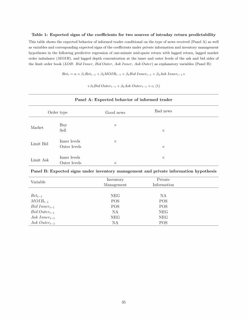
Table 1: Expected signs of the coefficients for two sources of intraday return predictabilityThis table shows the expected behavior of informed trader conditional on the type of news received (Panel A) as wellas variables and corresponding expected signs of the coefficients under private information and inventory managementhypotheses in the following predictive regression of one-minute mid-quote return with lagged return, lagged marketorder imbalance (MOIB), and lagged depth concentration at the inner and outer levels of the ask and bid sides ofthe limit order book (LOB: Bid Inner, Bid Outer, Ask Inner, Ask Outer) as explanatory variables (Panel B):

Rett = α+ β1Rett−1 + β2MOIBt−1 + β3Bid Innert−1 + β4Ask Innert−1+

+β5Bid Outert−1 + β6Ask Outert−1 + εt (1)

Panel A: Expected behavior of informed trader

Order type Good news Bad news

Market Buy ×Sell ×

Limit Bid Inner levels ×Outer levels ×

Limit Ask Inner levels ×Outer levels ×

Panel B: Expected signs under inventory management and private information hypothesis

Variable InventoryManagement

PrivateInformation

Rett−1 NEG NAMOIBt−1 POS POSBid Innert−1 POS POSBid Outert−1 NA NEGAsk Innert−1 NEG NEGAsk Outert−1 NA POS

35

Tab

le2:

Variables

descriptions

Thist

ableshow

sthe

descrip

tionof

thevaria

bles

used

inthepa

per.

Pane

lAshow

svariables

fort

hefirst

part

ofthean

alysisregardingintrad

ayreturn

pred

ictability

from

marketan

dlim

itorde

rflo

ws.

Pane

lBshow

svaria

bles

forthesecond

part

ofthean

alysis

regardingtheeff

ectof

algorit

hmic

trad

ingon

thechoice

mad

eby

inform

edtrad

er.

Pan

elA:Intrad

ayreturn

pred

ictability

Varia

ble

Descriptio

n

Ret

One-m

inutelog-returnsba

sedon

theprevailin

gmid-quo

tes(average

ofthebidan

daskprices)at

theendof

theon

e-minuteinterval

atindividu

alstocklevel.

MO

IB

One-m

inutemarketorderim

balance(bu

yvo

lumeminus

sellvo

lume)

atindividu

alstocklevel.

Bid

In

ner

(Ask

In

ner)

Basedon

asnap

shot

ofthebid(ask)sid

eof

thelim

itorderbo

okat

theendof

each

one-minuteinterval,I

defin

etheinnerdepthconcentrationas

cumulativedepthlyingbe

tweenmid-quo

tean

don

e-third

ofthetotal

distan

cebe

tween10th

availablelim

itpricean

dmid-quo

terelativ

eto

thetotalc

umulativedepthof

thebid

(ask)sid

eof

thelim

itorderbo

ok.

Bid

Oute

r(A

skO

ute

r)

Basedon

asnap

shot

ofthebid(ask)sid

eof

thelim

itorderbo

okat

theendof

each

one-minuteinterval,I

defin

etheou

terdepthconcentrationas

cumulativedepthlyingbe

tweenon

e-third

andtw

o-third

sof

thetotal

distan

cebe

tween10th

availablelim

itpricean

dmid-quo

terelativ

eto

thetotalc

umulativedepthof

thebid

(ask)sid

eof

thelim

itorderbo

ok.

Pan

elB:Effe

ctof

algorithmic

trad

ingactivity

Varia

ble

Descriptio

n

AT

The

daily

numbe

rof

best

bid-off

erqu

oteup

datesrelativ

eto

theda

ilytrad

ingvo

lume(in

$10,000)

onstock-da

yba

sis.

MC

AP

Mon

thly

averageof

theda

ilylogof

marketcapitalizationin

billion

sat

individu

alstocklevel.

1/P

RC

Inverseof

mon

thly

averageof

theda

ilyclosingpriceat

individu

alstocklevel.

Turn

over

Mon

thly

averageof

theda

ilyan

nualized

turnover

atindividu

alstocklevel.

Vol

ati

lity

Squa

reroot

ofmon

thly

averageof

theda

ilyhigh

minus

low

rang

eat

individu

alstocklevel.

36

Tab

le3:

Descriptive

statistics

Thistableshow

ssummarystatistic

sof

one-minutemid-quo

tereturns,marketorde

rim

balance(M

OIB),an

dde

pthconcentrationat

theinne

ran

dou

terlevelsof

theaskan

dbidside

sof

thelim

itorde

rbo

okfortheNYSE

-listed

common

stocks

durin

g2002-2010.

Returns

arerepo

rted

inba

sispo

ints,m

arketo

rder

imba

lanceis

repo

rted

inUSD

,dep

thconcentrationat

theinne

rand

outerlevelsisr

eportedin

percentage,c

utoff

points

betw

eeninne

rand

outerlevelsa

rerepo

rted

inpe

rcentage

relativ

eto

themid-quo

te.Fo

rde

taile

dde

scrip

tionof

thevaria

bles

please

referto

Table2.

Tocompu

tesummarystatistic

s,Ifollow

thefollo

wingproced

ure.

First,

Iwinsoriz

eon

e-minuteob

servations

perstock-da

yat

the1%

and99%

levels.Se

cond

,the

averageof

theon

e-minuteob

servations

perstock-da

yis

calculated

for

each

varia

ble.

Third,Iwinsoriz

eda

ilyob

servations

atthe1%

and99%

levels

forthewho

lesamplepe

riod.

The

n,thesummarystatistic

sacross

alls

tock-days

arecompu

tedforeach

varia

ble.

Alltheresults

arerepo

rted

forthewho

lesamplepe

riod(P

anel

A:J

an-2002un

tillD

ec-2010)

andforthetw

osub-samplepe

riods

(Pan

elB:J

an-2002un

tillJ

un-2006an

dPa

nelC

:Jul-2006un

tillD

ec-2010).To

beinclud

edin

thesample,

astockshou

ldha

veNYSE

asits

prim

aryexchan

ge.

Dataon

common

stocks

andprim

aryexchan

gecode

areob

tained

from

CRSP

databa

se(P

RIM

EXCH=N,a

ndSH

RCD=10

or11,E

XCHCD

=1or

31).

Dataon

consolidated

trad

es,q

uotes,

and10

best

levels

ofthelim

itorde

rbo

okareprov

ided

byTRT

H.

Pan

elA:Ja

n-2002

untillDec-2010

Ret

MO

IB

Bid

In

ner

Ask

In

ner

Bid

Oute

rA

skO

ute

rB

idC

uto

ff

Ask

Cuto

ff

Mean

-0.003

4,13

3.34

32.19%

31.49%

31.20%

31.36%

-1.43%

1.47

%St.Dev.W

ithin

0.58

315

,484

.35

18.74%

17.47%

11.14%

10.92%

2.34

%2.63

%St.Dev.Be

tween

0.16

05,93

0.18

11.43%

11.05%

6.40

%5.99

%2.27

%2.86

%Pan

elB:Ja

n-2002

untillJu

n-2006

Ret

MO

IB

Bid

In

ner

Ask

In

ner

Bid

Oute

rA

skO

ute

rB

idC

uto

ff

Ask

Cuto

ff

Mean

0.01

47,72

5.14

45.31%

42.66%

24.69%

25.49%

-2.45%

2.34

%St.Dev.W

ithin

0.49

315

,263

.00

16.15%

15.35%

9.65

%9.45

%2.83

%3.20

%St.Dev.Be

tween

0.18

19,59

0.36

11.70%

10.60%

6.09

%5.11

%3.01

%3.78

%Pan

elC:Ju

l-2006

untillDec-2010

Ret

MO

IB

Bid

In

ner

Ask

In

ner

Bid

Oute

rA

skO

ute

rB

idC

uto

ff

Ask

Cuto

ff

Mean

-0.020

840.15

20.47%

21.53%

37.03%

36.59%

-0.51%

0.68

%St.Dev.W

ithin

0.66

414

,398

.41

10.64%

11.45%

8.69

%9.11

%0.72

%1.28

%St.Dev.Be

tween

0.08

13,20

0.42

10.04%

10.71%

5.83

%6.28

%0.87

%1.34

%

37

Tab

le4:

Estim

ationresultsof

theintrad

ayreturn

pred

ictabilityfrom

MO

IB

and

LO

B

Thistableshow

stheaverageestim

ation

results

ofpred

ictiv

eregression

sof

one-minutemid-quo

tereturnson

lagged

returns,

lagged

marketorde

rim

balance

(MOIB),an

dlagged

depthconcentrationat

theinne

ran

dou

terlevelsof

theaskan

dbidside

sof

thelim

itorde

rbo

okforNYSE

-listed

common

stocks

durin

gthe

samplepe

riod(2002-2010):

Ret

t=α

+β

1Ret

t−1

+β

2MOIB

t−1

+β

3BidInner

t−1

+β

4AskInner

t−1

+β

5BidOuter t

−1

+β

6AskOuter t

−1

+ε t

(1)

Irunthis

regression

onthestock-da

yba

sis.

The

tablerepo

rtsaveragecoeffi

cients

together

with

averageNew

ey-W

estt-statistic

s(P

anel

A),

andad

justed

R2

decompo

sitio

n(P

anel

B).

Coefficientfororde

rim

balanceis

scaled

by10

9.Allothe

rcoeffi

cients

arescaled

by10

4.To

compu

teaverageNew

ey-W

estt-statistic

,Iuseatim

e-serie

sof

estim

ated

coeffi

cients

foreach

stockto

compu

teNew

ey-W

estt-statistic

san

daverageit

across

stocks.Individu

alregression

t-statistic

sare

used

tode

term

inetheprop

ortio

nof

regression

sthat

repo

rtsign

ificant

coeffi

cients

(eith

erpo

sitiv

eor

negativ

e).The

orde

ringof

thevaria

bles

used

tode

compo

sethead

justed

R2is

identic

alto

theorde

rin

which

they

appe

arin

thetable.

The

last

tworowsshow

thetotaln

umbe

rof

stock-da

yob

servations

andtheaverage

numbe

rof

stocks

perda

y.To

beinclud

edin

thesample,

astockshou

ldha

veNYSE

asits

prim

aryexchan

ge.Dataon

common

stocks

andprim

aryexchan

gecode

areob

tained

from

CRSP

databa

se(P

RIM

EXCH=N,a

ndSH

RCD=10

or11,E

XCHCD

=1or

31).

Dataon

consolidated

trad

es,q

uotes,

and10

best

levels

ofthe

limit

orde

rbo

okareprov

ided

byTRT

H.*

**,**,*indicate

sign

ificanceat

the1%

,5%,a

nd10%

levels,r

espe

ctively.

Pan

elA:Coefficientestimates

(dep

ende

ntvariab

le:

Ret

t)

Jan-2002

untillD

ec-2010

Jan-2002

untillJ

un-2006

Jul-2

006un

tillD

ec-2010

%of

significan

tan

d%

ofsig

nifican

tan

d%

ofsig

nifican

tan

d

Coef

Posit

ive

Negative

Coef

Posit

ive

Negative

Coef

Posit

ive

Negative

Con

stan

t0.048

8.29%

7.74%

0.111

8.50%

7.50%

-0.006

8.10%

7.96%

(0.46)

(0.73)

(0.00)

Ret

t−1

-0.011***

14.57%

20.23%

-0.013***

13.31%

20.24%

-0.009***

15.69%

20.21%

(-4.86)

(-4.86)

(-3.19)

MO

IB

t−1

4.650***

26.43%

2.48%

3.145***

24.87%

2.46%

6.278***

27.81%

2.50%

(18.87)

(15.17)

(15.08)

Bid

In

ner

t−1

1.894***

16.02%

4.80%

1.714***

16.31%

4.41%

2.055***

15.76%

5.14%

(9.66)

(9.24)

(7.23)

Ask

In

ner

t−1

-2.021***

4.41%

17.65%

-2.113***

3.41%

19.56%

-1.915***

5.30%

15.95%

(-11.00)

(-12.38)

(-6.95)

Bid

Oute

r t−

1-0.155

7.21%

8.09%

0.154

7.92%

7.14%

-0.434**

6.57%

8.93%

(-0.95)

(0.73)

(-2.15)

Ask

Oute

r t−

10.113

8.08%

7.27%

-0.168

7.20%

7.88%

0.356*

8.87%

6.74%

(0.74)

(-0.88)

(1.81)

Adjusted

R2

1.64%

1.71%

1.58%

#of

stock-da

ys2,740,593

1,291,413

1,448,989

Average#

ofstocks

1,228

1,167

1,289

38

Tab

le4:

Estim

ationresultsof

theintrad

ayreturn

pred

ictabilityfrom

MO

IB

and

LO

B(con

tinu

ed)

Pan

elB:Adjusted

R2de

compo

sition

(dep

ende

ntvariab

le:

Ret

t)

Jan-2002

untillD

ec-2010

Jan-2002

untillJ

un-2006

Jul-2

006un

tillD

ec-2010

Adjusted

R2

Adjusted

R2

Adjusted

R2

Absolute

Relative

Absolute

Relative

Absolute

Relative

Con

stan

t

Ret

t−1

0.53%

32.38%

0.54%

31.32%

0.53%

33.38%

MO

IB

t−1

0.34%

20.66%

0.33%

19.28%

0.35%

21.98%

Bid

In

ner

t−1

0.21%

13.05%

0.23%

13.66%

0.20%

12.45%

Ask

In

ner

t−1

0.24%

14.74%

0.28%

16.08%

0.21%

13.42%

Bid

Oute

r t−

10.16%

9.57%

0.17%

9.86%

0.15%

9.34%

Ask

Oute

r t−

10.16%

9.60%

0.17%

9.79%

0.15%

9.44%

Tot

al

In

ner

0.45%

27.79%

0.51%

29.74%

0.41%

25.87%

Tot

al

Oute

r0.32%

19.17%

0.34%

19.65%

0.30%

18.78%

Tot

al

LO

B0.77%

46.96%

0.85%

49.39%

0.71%

44.65%

Tot

al

1.64%

100.00%

1.71%

100.00%

1.58%

100.00%

#of

stock-da

ys2,740,593

1,291,413

1,448,989

Average#

ofstocks

1,228

1,167

1,289

39

Tab

le5:

Estim

ationresultsof

theintrad

ayreturn

pred

ictabilityfrom

surprisesin

MO

IB

and

LO

B

Thistableshow

stheaverageestim

ationresults

ofpred

ictiv

eregression

sof

one-minutemid-quo

tereturnson

lagged

surpris

esin

returns,lagged

surpris

esin

market

orde

rimba

lance(M

OIB),an

dlagged

surpris

esin

depthconcentrationat

theinne

rand

outerlevelsof

theaskan

dbidside

sof

thelim

itorde

rboo

kforNYSE

-listed

common

stocks

durin

gthesamplepe

riod(2002-2010):

Ret

t=α

+β

1Ret

U t−1

+β

2MOIB

U t−1

+β

3BidInner

U t−1

+β

4AskInner

U t−1

+β

5BidOuterU t−

1+β

6AskOuterU t−

1+ε t

(3)

Surpris

esarecompu

tedas

residu

alvalues

from

VAR

(k)regression

perstock-da

y,nu

mbe

rof

lags,k

,can

take

values

from

1to

5an

disselected

byAIC

crite

ria(see

equa

tion2).Su

perscriptU

indicatesthat

this

aresidu

alvaluefrom

VAR

(k).

Irunthis

regression

onthestock-da

yba

sis.

The

tablerepo

rtsaveragecoeffi

cients

together

with

averageNew

ey-W

estt-statistic

s(P

anel

A),

andad

justed

R2de

compo

sitio

n(P

anel

B).

Coefficientfororde

rim

balanceis

scaled

by10

9.Allothe

rcoeffi

cients

arescaled

by10

4.To

compu

teaverageNew

ey-W

estt-statistic

,Iuseatim

e-serie

sof

estim

ated

coeffi

cients

foreach

stockto

compu

teNew

ey-W

est

t-statistic

san

daverageit

across

stocks.Individu

alregression

t-statistic

sareused

tode

term

inetheprop

ortio

nof

regression

sthat

repo

rtsign

ificant

coeffi

cients

(eith

erpo

sitiv

eor

negativ

e).The

orde

ringof

thevaria

bles

used

tode

compo

sethead

justed

R2isidentic

alto

theorde

rin

which

they

appe

arin

thetable.

The

last

tworowsshow

thetotaln

umbe

rof

stock-da

yob

servations

andtheaveragenu

mbe

rof

stocks

perda

y.To

beinclud

edin

thesample,

astockshou

ldha

veNYSE

asits

prim

aryexchan

ge.Dataon

common

stocks

andprim

aryexchan

gecode

areob

tained

from

CRSP

databa

se(P

RIM

EXCH=N,a

ndSH

RCD=10

or11,E

XCHCD

=1or

31).

Dataon

consolidated

trad

es,q

uotes,

and10

best

levels

ofthelim

itorde

rbo

okareprov

ided

byTRT

H.*

**,**,*indicate

sign

ificanceat

the1%

,5%,

and10%

levels,r

espe

ctively.

Pan

elA:Coefficientestimates

(dep

ende

ntvariab

le:

Ret

t)

Jan-2002

untillD

ec-2010

Jan-2002

untillJ

un-2006

Jul-2

006un

tillD

ec-2010

%of

significan

tan

d%

ofsig

nifican

tan

d%

ofsig

nifican

tan

d

Coef

Posit

ive

Negative

Coef

Posit

ive

Negative

Coef

Posit

ive

Negative

Con

stan

t-0.002

6.72%

6.19%

0.013

7.14%

6.26%

-0.017

6.35%

6.13%

(0.10)

(0.73)

(-0.57)

Ret

U t−1

-0.015***

13.38%

20.56%

-0.020***

11.86%

21.18%

-0.011***

14.74%

20.01%

(-6.21)

(-6.34)

(-3.74)

MO

IB

U t−1

4.774***

25.25%

2.27%

3.213***

23.75%

2.34%

6.459***

26.58%

2.20%

(18.83)

(14.99)

(15.19)

Bid

In

ner

U t−1

2.520***

15.00%

4.62%

2.617***

15.31%

4.19%

2.497***

14.73%

5.01%

(9.51)

(8.96)

(7.11)

Ask

In

ner

U t−1

-2.571***

4.36%

16.24%

-2.775***

3.51%

17.74%

-2.394***

5.12%

14.90%

(-10.45)

(-11.08)

(-7.01)

Bid

Oute

rU t−1

-0.004

7.04%

7.76%

0.601

7.58%

6.76%

-0.434*

6.56%

8.66%

(-0.31)

(1.26)

(-1.86)

Ask

Oute

rU t−1

0.049

7.76%

7.05%

-0.273

6.89%

7.44%

0.315

8.54%

6.70%

(0.38)

(-1.02)

(1.47)

Adjusted

R2

1.50%

1.57%

1.44%

#of

stock-da

ys2,739,445

1,290,389

1,448,865

Average#

ofstocks

1,228

1,166

1,289

40

Tab

le5:

Estim

ationresultsof

theintrad

ayreturn

pred

ictabilityfrom

surprisesin

MO

IB

and

LO

B(con

tinu

ed)

Pan

elB:Adjusted

R2de

compo

sition

(dep

ende

ntvariab

le:

Ret

t)

Jan-2002

untillD

ec-2010

Jan-2002

untillJ

un-2006

Jul-2

006un

tillD

ec-2010

Adjusted

R2

Adjusted

R2

Adjusted

R2

Absolute

Relative

Absolute

Relative

Absolute

Relative

Con

stan

t

Ret

U t−1

0.48%

31.87%

0.49%

31.42%

0.47%

32.29%

MO

IB

U t−1

0.31%

20.92%

0.31%

19.83%

0.32%

21.97%

Bid

In

ner

Ut−

10.20%

13.40%

0.22%

13.81%

0.19%

13.00%

Ask

In

ner

Ut−

10.21%

14.25%

0.24%

15.34%

0.19%

13.20%

Bid

Oute

rUt−

10.15%

9.79%

0.15%

9.83%

0.14%

9.77%

Ask

Oute

rUt−

10.15%

9.77%

0.15%

9.78%

0.14%

9.78%

Tot

al

In

ner

U0.41%

27.65%

0.46%

29.15%

0.38%

26.20%

Tot

al

Oute

rU0.30%

19.56%

0.30%

19.61%

0.28%

19.55%

Tot

al

LO

BU

0.71%

47.21%

0.76%

48.76%

0.66%

45.75%

Tot

alU

1.50%

100.00%

1.57%

100.00%

1.44%

100.00%

#of

stock-da

ys2,739,445

1,290,389

1,448,865

Average#

ofstocks

1,228

1,166

1,289

41

Tab

le6:

Second

stageregression

:Im

pact

ofalgo

rithmic

trad

ingactivity

onintrad

ayreturn

pred

ictability

Thistableshow

stheim

pact

ofalgorit

hmic

trad

ingactiv

ityon

intrad

ayreturn

pred

ictabilityfrom

thelim

itorde

rbo

ok:

Yi,

t=α

i+γ

t+β

1AT

i,t

+β

2MCAP

i.m

−1

+β

3(1/PRC

i,m

−1)+

β4Turnover

i,m

−1

+β

5Volatility

i,m

−1

+ε i

,t(4

)

Asproxyforalgorit

hmic

trad

ingactiv

ityIuseda

ilynu

mbe

rof

best

bid-off

erqu

oteup

datespe

r$10,000of

daily

trad

ingvolume(AT

i,t).

Inorde

rto

identify

causal

effectof

algorit

hmic

trad

ingactiv

ity,I

instrumentitwith

staggeredintrod

uctio

nof

NYSE

Hyb

rid.The

setof

instruments

includ

ealle

xplana

tory

varia

bles

with

AT

i,tsubstit

uted

byHybrid

i,t.Icontrolforda

ilymarketcapitalization,

price,

turnover,an

dvo

latility

averaged

over

theprevious

calend

armon

th.The

specificatio

ninclud

esstock(α

i)an

dda

y(γ

t)fix

edeff

ects.Stan

dard

errors

aread

justed

fordo

uble

clusterin

g.Pa

nelA

repo

rtstheeff

ectof

algorit

hmic

trad

ing

onthecoeffi

cients

from

pred

ictiv

eregression

s.Pa

nelB

repo

rtstheeff

ectof

algorit

hmic

trad

ingon

theincrem

entala

djustedR

2from

pred

ictiv

eregression

s.The

last

tworowsin

each

pane

lsho

wthetotaln

umbe

rof

stock-da

yob

servations

andtheaveragenu

mbe

rof

stocks

perda

y.The

estim

ationpe

riodis

Jun-2006

untill

May-2007.

Tobe

includ

edin

thesample,

astockshou

ldha

veNYSE

asits

prim

aryexchan

gean

dha

veCRSP

data

availableforallda

ysun

derconsideration.

Dataon

common

stocks

andprim

aryexchan

gecode

areob

tained

from

CRSP

databa

se(P

RIM

EXCH=N,an

dSH

RCD=10

or11,EXCHCD

=1or

31).

Data

onconsolidated

trad

es,qu

otes,an

d10

best

levels

ofthelim

itorde

rbo

okareprovided

byTRT

H.Dataon

NYSE

Hyb

ridintrod

uctio

ncomes

from

Terren

ceHen

dersho

tt’s

web

site.***,**,*

indicate

sign

ificanceat

the1%

,5%,a

nd10%

levels,r

espe

ctively.

Pan

elA:Effe

ctof

algorithmic

trad

ingon

coeffi

cients

Ret

U i,t−

1M

OIB

U i,t−

1B

idIn

ner

U i,t−

1A

skIn

ner

U i,t−

1B

idO

ute

rU i,t−

1A

skO

ute

rU i,t−

1

AT

i,t

-0.004

***

0.095*

*0.33

7***

-0.275

***

-0.006

0.00

1(-3.67

)(2.40)

(9.21)

(-6.66

)(-0.17

)(0.05)

ln(M

CA

P) i,

m−

1-0.010

***

0.16

21.15

8***

-1.026**

*0.18

2*-0.153

(-2.78

)(1.13)

(8.28)

(-7.19

)(1.71)

(-1.30

)1/

PR

Ci,

m−

1-0.321

***

54.778

***

8.28

8**

-7.782

*8.49

0**

-4.437

(-3.28

)(11.14

)(1.97)

(-1.82)

(2.47)

(-1.32

)T

urn

over

i,m

−1

-0.045

***

-1.594**

*1.37

3***

-0.952

***

0.02

2-0.029

(-8.02

)(-7.68

)(6.70)

(-4.45

)(0.12)

(-0.18

)V

olati

lity

i,m

−1

0.74

8***

56.901

***

-4.218

-0.311

-9.770

**9.04

8**

(6.13)

(10.24

)(-0.80

)(-0.06

)(-2.45

)(2.31)

StockFE

YES

YES

YES

YES

YES

YES

Day

FEYES

YES

YES

YES

YES

YES

Dou

bleclusterin

gYES

YES

YES

YES

YES

YES

R2

0.14

0.35

0.06

0.06

0.01

0.01

#of

stock-da

ys29

6,13

029

6,13

029

6,13

029

6,13

029

6,13

029

6,13

0Av

erag

e#

ofstocks

1,18

01,18

01,18

01,18

01,18

01,18

0

42

Tab

le6:

Second

stageregression

(con

tinu

ed)

Pan

elB:Effe

ctof

algorithmic

trad

ingon

increm

entalAdjusted

R2

Adj

R2 i,

tR

etU i,

t−1

MO

IB

U i,t−

1B

idIn

ner

U i,t−

1A

skIn

ner

U i,t−

1B

idO

ute

rU i,t−

1A

skO

ute

rU i,t−

1

AT

BB

Oi,

t0.21

1***

0.08

0***

0.05

2***

0.02

5***

0.02

6***

0.00

7**

0.00

6*(9.11)

(7.93)

(8.20)

(5.64)

(5.26)

(2.17)

(1.76)

ln(M

CA

P) i,

m−

10.38

0***

0.23

4***

0.00

40.04

9***

0.07

9***

0.00

1-0.005

(6.31)

(7.88)

(0.24)

(4.05)

(5.72)

(0.09)

(-0.60

)1/

PR

Ci,

m−

1-4.410

**-1.681

**-1.461

***

-0.692**

-0.550

0.16

30.12

9(-2.53

)(-2.19

)(-2.83

)(-2.08

)(-1.41

)(0.68)

(0.50)

Turn

over

i,m

−1

1.20

9***

0.50

8***

0.26

0***

0.13

2***

0.14

0***

0.04

7***

0.03

7**

(10.72

)(9.88)

(8.52)

(5.89)

(5.59)

(3.07)

(2.12)

Vol

ati

lity

i,m

−1

-27.37

2***

-11.06

5***

-4.728

***

-3.027

***

-3.631

***

-1.430

***

-1.355

***

(-12

.40)

(-10

.42)

(-7.97

)(-7.12

)(-7.55)

(-4.73

)(-4.34

)

StockFE

YES

YES

YES

YES

YES

YES

YES

Day

FEYES

YES

YES

YES

YES

YES

YES

Dou

bleclusterin

gYES

YES

YES

YES

YES

YES

YES

R2

0.06

0.04

0.06

0.03

0.04

0.02

0.02

#of

stock-da

ys29

6,13

029

6,13

029

6,13

029

6,13

029

6,13

029

6,13

0296,13

0Av

erag

e#

ofstocks

1,18

01,18

01,18

01,18

01,18

01,18

01,18

0

43

Tab

le7:

Realiz

edvolatilitypo

rtfolio

san

dintrad

ayreturn

pred

ictabilityfrom

surprisesin

MO

IB

and

LO

B

Thistableshow

stheaverageestim

ationresults

ofpred

ictiv

eregression

sof

one-minutemid-quo

tereturnson

lagged

surpris

esin

returns,lagged

surpris

esin

market

orde

rimba

lance(M

OIB),an

dlagged

surpris

esin

depthconcentrationat

theinne

rand

outerlevelsof

theaskan

dbidside

sof

thelim

itorde

rboo

kforNYSE

-listed

common

stocks

durin

gthesamplepe

riod(2002-2010):

Ret

t=α

+β

1Ret

U t−1

+β

2MOIB

U t−1

+β

3BidInner

U t−1

+β

4AskInner

U t−1

+β

5BidOuterU t−

1+β

6AskOuterU t−

1+ε t

(3)

Surpris

esarecompu

tedas

residu

alvalues

from

VAR

(k)regression

perstock-da

y,nu

mbe

rof

lags,k

,can

take

values

from

1to

5an

dis

selected

byAIC

crite

ria.

Supe

rscriptU

indicatesthat

thisaresidu

alvaluefrom

VAR

(k).

Irunthisregression

onthestock-da

yba

sis.

Foreach

dayIsort

allthe

stocks

into

four

portfolio

sba

sedon

one-da

ylagged

realized

volatility

(realized

volatility

iscompu

tedfrom

one-minutemid-quo

tereturns).The

tablerepo

rtsaveragecoeffi

cients

together

with

averageNew

ey-W

estt-statistic

s(P

anel

A),an

dad

justed

R2de

compo

sitio

n(P

anel

B).Coefficientfororde

rim

balanceis

scaled

by10

9.Allothe

rcoeffi

cients

arescaled

by10

4.To

compu

teaverageNew

ey-W

estt-statistic

,Iuseatim

e-serie

sof

estim

ated

coeffi

cients

foreach

stockto

compu

teNew

ey-W

estt-statistic

san

daverageitacross

stocks.The

orde

ringof

thevaria

bles

used

tode

compo

sethead

justed

R2isidentic

alto

theorde

rin

which

they

appe

arin

thetable.

The

last

two

rowsshow

thetotaln

umbe

rof

stock-da

yob

servations

andtheaveragenu

mbe

rof

stocks

perda

y.To

beinclud

edin

thesample,

astockshou

ldha

veNYSE

asits

prim

aryexchan

ge.Dataon

common

stocks

andprim

aryexchan

gecode

areob

tained

from

CRSP

databa

se(P

RIM

EXCH=N,a

ndSH

RCD=10

or11,E

XCHCD

=1or

31).

Dataon

consolidated

trad

es,q

uotes,

and10

best

levels

ofthelim

itorde

rbo

okareprov

ided

byTRT

H.*

**,**,*indicate

sign

ificanceat

the1%

,5%,

and10%

levels,r

espe

ctively.

Pan

elA:Coefficientestimates

(dep

ende

ntvariab

le:

Ret

t)

RV1(lo

w)

RV2

RV3

RV4(high)

Con

stan

t0.00

50.00

3-0.001

-0.016

(0.06)

(0.01)

(0.00)

(-0.17

)R

etU t−

1-0.011

*-0.009

-0.013

**-0.027

***

(-1.70

)(-1.51

)(-2.03

)(-2.81

)M

OIB

U t−1

1.17

5***

2.39

7***

4.42

0***

11.630

***

(7.40)

(7.28)

(6.74)

(6.10)

Bid

In

ner

U t−1

1.64

2***

2.08

9***

2.58

5***

3.78

1***

(4.22)

(4.35)

(4.23)

(4.08)

Ask

In

ner

U t−1

-1.714

***

-2.135

***

-2.625

***

-3.813

***

(-4.61

)(-4.75

)(-4.71

)(-4.55

)B

idO

ute

rU t−1

-0.072

-0.075

-0.005

0.156

(-0.14

)(-0.21

)(-0.08

)(0.08)

Ask

Oute

rU t−1

0.10

20.09

40.06

3-0.068

(0.25)

(0.24)

(0.11)

(-0.12

)

Adjusted

R2

1.50

%1.44

%1.47

%1.68

%

#of

stock-da

ys68

4,53

168

3,13

868

3,80

168

2,74

2Av

erag

e#

ofstocks

307

306

307

306

44

Tab

le7:

Realized

volatilitypo

rtfolio

san

dintrad

ayreturn

pred

ictabilityfrom

surprisesin

MO

IB

and

LO

B(con

tinu

ed)

Pan

elB:Adjusted

R2de

compo

sition

(dep

ende

ntvariab

le:

Ret

t)

RV1(lo

w)

RV2

RV3

RV4(high)

Adjusted

R2

Adjusted

R2

Adjusted

R2

Adjusted

R2

Absolute

Relative

Absolute

Relative

Absolute

Relative

Absolute

Relative

Con

stan

t

Ret

U t−1

0.48

%32.07%

0.45

%31

.67%

0.46%

31.43%

0.54

%32

.15%

MO

IB

U t−1

0.29

%19.42%

0.29

%20

.08%

0.31%

21.01%

0.38

%22

.88%

Bid

In

ner

Ut−

10.21

%14.00%

0.20

%13

.82%

0.20

%13

.44%

0.21

%12

.52%

Ask

In

ner

Ut−

10.22

%14.95%

0.21

%14

.78%

0.21

%14

.35%

0.22

%13

.17%

Bid

Oute

rUt−

10.15

%9.78

%0.14

%9.80

%0.15

%9.92

%0.16

%9.68

%A

skO

ute

rUt−

10.15

%9.78

%0.14

%9.86

%0.14

%9.84

%0.16

%9.60

%

Tot

al

In

ner

U0.43

%28.95%

0.41

%28

.60%

0.41

%27

.79%

0.43

%25

.69%

Tot

al

Oute

rU0.30

%19.56%

0.28

%19

.66%

0.29

%19

.76%

0.32

%19

.28%

Tot

al

LO

BU

0.73

%48.51%

0.69

%48

.26%

0.70

%47

.55%

0.75

%44

.97%

Tot

alU

1.50

%10

0.00

%1.44

%10

0.00

%1.47

%10

0.00

%1.68%

100.00

%

#of

stock-da

ys68

4,53

1683,13

868

3,80

168

2,74

2Av

erag

e#

ofstocks

307

306

307

306

45

Figure 1: Limit order book composition

This figure shows the equally-weighted average of the depth concentration at the inner and outer levels for the askand bid sides of the limit order book for the NYSE-listed common stocks during 2002-2010. Please refer to Table 2 fordetailed variables description. I use the following procedure to construct time-series of the equally-weighted averages ofthe variables. First, I winsorize one-minute observations per stock-day at the 1% and 99% levels. Second, the averageof the one-minute observations per stock-day is calculated for each variable. Third, I winsorize daily observations atthe 1% and 99% levels for the whole sample period. Then, the summary statistics across all stock-days are computedfor each variable. Then, I plot one-month moving average of each variable. To be included in the sample, a stockshould have NYSE as its primary exchange. Data on common stocks and primary exchange code are obtained fromCRSP database (PRIMEXCH=N, and SHRCD=10 or 11, EXCHCD =1 or 31). Data on consolidated trades, quotes,and 10 best levels of the limit order book are provided by TRTH.

Panel A: Depth concentration at the inner and outer levels of the limit order book

Panel B: Cutoff point between inner and outer levels of the limit order book

46

Figure 2: NYSE Hybrid Market introduction

This figure shows the staggered way of NYSE Hybrid Market introduction for the stocks included in the analysisfrom October 1, 2006 to January 31, 2007. To be included in the sample, a stock should have NYSE as its primaryexchange and have CRSP daily data available for the period from June 2006 to May 2007. Data on common stocksand primary exchange code are obtained from CRSP database (PRIMEXCH=N, and SHRCD=10 or 11, EXCHCD=1 or 31). Data on Hybrid introduction are from Terrence Hendershott’s website.

47