Randomized Algorithms - Deterministic and Randomized Quicksort

Intraclass Correlation Values for Planning Group Randomized Trials in Education
By
Larry V. Hedges Northwestern University
And
Eric C. Hedberg
University of Chicago

Intraclass correlations in education 2
Abstract
Experiments that assign intact groups to treatment conditions are increasingly
common in social research. In educational research, the groups assigned are often
schools. The design of group randomized experiments requires knowledge of the
intraclass correlation structure to compute statistical power and sample sizes required to
achieve adequate power. This paper provides a compilation of intraclass correlation
values of academic achievement and related covariate effects that could be used for
planning group randomized experiments in education. It also provides variance
component information that is useful in planning experiments involving covariates. The
use of these values to compute statistical power of group randomized experiments is
illustrated.

Intraclass correlations in education 3
Intraclass Correlation Values for Planning Group Randomized Trials in Education
Many social interventions operate at a group level by altering the physical or
social conditions. In such cases, it may be difficult or impossible to assign individuals to
receive different intervention conditions. In such cases, field experiments often assign
entire intact groups (such as sites, classrooms, or schools) to the same treatment, with
different intact groups being assigned to different treatments. Because these intact
groups correspond to what statisticians call clusters in sampling theory, this design is
often called a group randomized or cluster randomized design. Cluster randomized trials
have been used extensively in public health and other areas of prevention science (see,
e.g., Donner and Klar, 2000; and Murray, 1998). Cluster randomized trials have become
more important in educational research more recently, following increased interest in
experiments to evaluate educational interventions (see, e.g., Mosteller and Boruch, 2002).
Methods for the design and analysis of group randomized trials have been discussed
extensively in Donner and Klar (2000),and Murray (1998).
The sampling of subjects into experiments via statistical clusters introduces
special considerations that need to be addressed in the analysis. For example, a sample
obtained from m clusters (such as classrooms or schools) of size n randomized into a
treatment group is not a simple random sample of nm individuals, even if it is based on a
simple random sample of clusters. Consequently the sampling distribution of statistics
based on such clustered samples is not the same as those based on simple random
samples of the same size. For example, suppose that the (total) variance of a population
with clustered structure (such as a population of students within schools) is σT2, and that

Intraclass correlations in education 4
this total variance is decomposable into a between cluster variance σB2 and a within
cluster variance σW2, so that σT
2 = σB2 + σW
2. Then the variance of the mean of a simple
random sample of size mn from that population would be σT2/mn. However, the variance
of the mean of a sample of m clusters, each of size n from that population (with the same
total sample size mn) would be [1 + (n – 1)ρ]σT2/mn, where ρ = σB
2/(σB2 + σW
2) is the
intraclass correlation. Thus the variance of the mean computed from a clustered sample
is larger by a factor of [1 + (n – 1)ρ], which is often called the design effect (Kish, 1965)
or variance inflation factor (Donner, Birkett, and Buck, 1981).
Several analysis strategies for cluster randomized trails are possible, but the
simplest is to treat the clusters as units of analysis. That is, to compute mean scores on
the outcome (and all other variables that may be involved in the analysis) and carry out
the statistical analysis as if the site (cluster) means were the data. If all cluster sample
sizes are equal, this approach provides exact tests for the treatment effect, but the tests
may have lower statistical power than would be obtained by other approaches (see, e.g.,
Blair and Higgins, 1986). More flexible and informative analyses are also available,
including analyses of variance using clusters as a nested factor (see, e.g., Hopkins, 1982)
and analyses involving hierarchical linear models (see e.g., Raudenbush and Bryk, 2002).
For general discussions of the design and analyses of cluster randomized experiments see
Murray (1998), Bloom, Bos, and Lee (1999), Donner and Klar (2000), Klar and Donner
(2001), Raudenbush and Bryk (2002), Murray, Varnell, & Blitstein (2004), or Bloom
(2005).
Wise experimental design involves the planning of sample sizes so that the test
for treatment effects has adequate statistical power to detect the smallest treatment effects

Intraclass correlations in education 5
that are of scientific or practical interest. There is an extensive literature on the
computation of statistical power, (e.g., Cohen, 1977; Kraemer and Thiemann, 1987;
Lipsey, 1990). Much of this literature involves the computation of power in studies that
use simple random samples. However methods for the computation of statistical power
of tests for treatment effects using the cluster mean as the unit of analysis (Blair and
Higgins, 1986), analysis of variance using clusters as a nested factor (Raudenbush, 1997),
and hierarchical linear model analyses (Sniders and Bosker, 1993) are available. For all
of these analyses, the noncentrality parameter required to compute statistical power
involves the intraclass correlation ρ. More complex analyses involving covariates require
corresponding information (covariate effects or the conditional intraclass correlations
after adjustment for covariates). Thus the computation of statistical power in cluster
randomized trials requires knowledge of the intraclass correlation ρ.
Because plausible values of ρ are essential for power and sample size
computations in planning cluster randomized experiments, there have been systematic
efforts to obtain information about reasonable values of ρ in realistic situations. One
strategy for obtaining information about reasonable values of ρ is to obtain these values
from cluster randomized trials that have been conducted. Murray and Blitstein (2003)
reported a summary of intraclass correlations obtained from 17 articles reporting cluster
randomized trials in psychology and public health and Murray, Varnell, and Blitstein
(2004) give references to 14 very recent studies that provide data on intraclass
correlations for health related outcomes. Another strategy for obtaining information on
reasonable values of ρ is to analyze sample surveys that have used a cluster sampling
design involving the clusters of interest. Gulliford, Ukoumunne, and Chinn (1999) and

Intraclass correlations in education 6
Verma and Lee (1996) presented values of intraclass correlations based on surveys of
health outcomes.
There is much less information about intraclass correlations appropriate for
studies of academic achievement as an outcome. Such information is badly needed to
inform the design of experiments that measure the effects of interventions on academic
achievement by randomizing schools (Schochet, 2005). One compendium of intraclass
correlation values based on five large urban school districts where randomized trials have
been conducted has recently become available (see Bloom, Richburg-Hayes, and Black,
2005). The purpose of this paper is to provide a comprehensive collection of intraclass
correlations of academic achievement based on national representative samples. We
hope that this compilation will be useful in choosing reference values for planning cluster
randomized experiments.
Dimensions of Designs Considered
Our analyses focused on intraclass correlations for designs involving assignment
of schools to treatments. Unfortunately, there is a wide variety of designs that might be
used to study education interventions, and each of these designs may have its own
intraclass correlation (or conditional intraclass correlation) structure. To attempt to
provide a reasonable coverage of the designs most likely to be of interest to researchers
planning educational experiments, we considered four dimensions of intervention designs.
The first dimension of the design is the grade level. The second dimension of the design
is what achievement domain (e.g., reading or mathematics) is the dependent variable.
The third dimension of the design is the set of covariates that were used in the analysis, if

Intraclass correlations in education 7
any. Finally, the fourth dimension was the socioeconomic (SES) or achievement status
of schools sampled in the overall population of schools. These four dimensions of
designs can vary independently. We examined all possible combinations of them.
Grade level of students and achievement domain. We examined each grade level
from Kindergarten through grade 12 and both mathematics and reading achievement at
each grade level, with one exception. The exception was reading achievement at grade
11, for which data on a national representative sample was not available to us.
Covariates used in the design. We consider four data analysis models involving
different covariate sets that we believe are likely to be of considerable interest to
educational researchers. The first, the unconditional model, involves testing of treatment
effects with no covariates. This is the minimal design, but one that is likely to be of
interest in many settings where the researcher has little opportunity to collect prior
information about the individuals participating in the experiment.
The second model, which we call the conditional model, involves testing of
treatment effects conditional on covariates that are ascriptive characteristics of students
frequently invoked in models of educational achievement, namely gender, race/ethnicity,
and socio-economic status. This design may be appropriate when the researcher can
obtain prior, contemporaneous, or retrospective data from administrative records
(appropriate because these covariates are unlikely to change).
The third model, which we call the residualized gain model, involves testing of
treatment effects using pretest scores on the same achievement domain (mathematics or
reading) as a covariate. This design is likely to be considerably more powerful than the
previous designs, but involves the additional cost of collecting another wave of test data

Intraclass correlations in education 8
and the additional organizational burden of making that data collection in a timely
manner.
The fourth model, which we call the conditional residualized gain model, involves
testing of treatment effects using the ascriptive characteristics of students (gender,
race/ethnicity, and socio-economic status) and pretest scores on the same achievement
domain as a covariates. This design combines both of the sets of covariates in the
previous design.
SES or achievement status of schools within their settings. Some experimenters
undoubtedly wish to use a representative sample of schools within whatever setting they
choose to study. Consequently one population of schools we considered was the entire
collection of schools within a setting.
Researchers sometimes make decisions to carry out their studies in schools that lie
within the middle range of outcomes, omitting schools that have had (or are reputed to
have had) the very poorest and the very best outcomes, on the rationale that neither the
very poorest schools nor the very best schools give a fair test of an intervention. We
operationalized this notion by ordering, on average achievement, the entire sample of
schools in a setting and selecting the middle 80% of the schools in each setting, omitting
the top and bottom 10% of the schools.
Some interventions are designed to be compensatory. Experimenters
investigating such interventions might choose only schools within a particular context
that have low mean achievement or large numbers of low SES students to evaluate the
intervention. We operationalized low achievement by ordering, on average achievement,
the entire sample of schools in a setting and selecting the lower 50% of the schools,

Intraclass correlations in education 9
omitting the upper 50% of the schools. We operationalized low SES by ordering, on
proportion of students eligible for free of reduced price lunch, the entire sample of
schools in a setting and selecting the upper 50% of the schools, omitting the bottom 50%
of the schools.
Datasets Used
The object of this paper is to estimate intraclass correlations and associated
variance components for academic achievement in reading and mathematics for the
United States and various subpopulations. Consequently we relied on data from
longitudinal surveys with national probability samples, all of which are described in
detail elsewhere. We chose longitudinal surveys because we wished to use achievement
data collected in earlier years as pretest data for evaluating conditional intraclass
correlation relevant for planning studies that would use a pretest as a covariate. In some
cases, more than one survey could have provided data on a given grade level. In such
cases, we report here results based on the survey with the largest sample size.
When it was possible to estimate intraclass correlations for the same grade and
achievement domain from more than one survey, we computed estimates from all surveys
from which it was possible. Generally, we found that the results agreed within sampling
error. The exception was that estimates from the second and third followups of the
Prospects samples tended to be least consistent with other estimates. This finding makes
sense in light of two principles. The first is that longitudinal studies suffer from attrition
and lose their representative character over time, so that followup waves, and particularly
second and third follow-ups, are no longer represent exactly the same population. The

Intraclass correlations in education 10
second is the more arguable principle that the Prospects study had larger differential
(non-random) attrition than other longitudinal studies considered here (which seems to be
supported by analyses of attrition).
The results reported for Kindergarten, grade 1, and grade 3 were obtained from
three waves of the Early Childhood Longitudinal Survey (ECLS). The ECLS is a
longitudinal study that obtained a national probability sample of Kindergarten children in
1591 schools in 1998 and followed them through the fifth grade (see Tourangeau, et al.,
2005). Achievement test data were collected in both Fall and Spring of Kindergarten
and first grade, and in Spring only in third and fifth grades. There was no data collection
in second and fourth grade. Thus Fall achievement test data collected in the same year
could serve as a pretest in Kindergarten and first grades, while data collected in the
Spring of the first grade served as pretest data for the third grade.
The results reported for grade 2 were obtained from the first followup to the first
grade (base year) sample and those reported for grades 4 to 6 were obtained from the
three follow-ups of the third grade (base year) sample in the Prospects study, and the
results in reading in grades 7 and 9 were obtained from the base year and the second
followup of the seventh grade sample in the Prospects study. Prospects was actually a set
of three longitudinal studies, starting with (base year) national probability samples of
children in 235, 240, and 137 schools, in grades 1, 3, and 7, respectively, conducted in
1991 (for a complete description of the study design, see Puma, et al., 1997).
Achievement test data was collected for three to four years thereafter for each sample.
Thus the three prospects studies collected data in grades 1 (both Fall and Spring), 2, and
3; grades 3, 4, 5, and 6; and 7, 8, and 9. There was pretest data in the base year for grade

Intraclass correlations in education 11
1, but no pretest data for the base years in grades 3 and 7. For all years except the base
year, the previous year’s achievement test data was used as a pretest and in grade 1 the
test data collected in fall served as a pretest.
The results reported on reading in grades 8, 10, and 12 and mathematics in grades
10 and 12 were obtained from the National Educational Longitudinal Study of the Eighth
Grade Class of 1988 (NELS: 88). NELS: 88 is a longitudinal study that began in 1988
with a national probability sample of eighth graders in 1050 schools and collected
reading and mathematics achievement test data when the students were in grades 8, 10,
and 12. Thus no pretest data was available for grade 8, but for the grade 10 the grade 8
data was used as a pretest and for grade 12 the grade 10 data was used as a pretest.
Finally, the results on mathematics in grades 7, 8, 9, and 11 were obtained from
the base year and follow-ups of the Longitudinal Study of American Youth (LSAY) (see
Miller, et al., 1992). The LSAY is a longitudinal study that began in 1987 with two
national probability samples, one of seventh graders in and one of tenth graders in 104
schools. Data were collected on mathematics and science achievement each year for four
years leading to samples from grades 7 to 12. There was no pretest data in grade 7, but
the previous year’s data served as the pretest for each subsequent year.
Analysis Procedures
The data analysis was carried out using STATA version 9.1’s “XTMIXED”
routine for mixed linear model analysis. For each sample and achievement domain,
analyses were carried out based on four different models, which we call the unconditional
model, the residualized gain model, the conditional model, and the conditional

Intraclass correlations in education 12
residualized gain model. We describe these explicitly below in hierarchical linear model
notation.
The unconditional model. The unconditional model involves no covariates at
either the individual or school (cluster) levels. The level-one model for the kth observation
in the jth school can be written as
0jk j jkY β ε= + ,
and the level two model for the intercept is
0 00j jζβ π= + ,
where εjk is an individual-level residual and ζj is a random effect of the jth cluster (a level-
two residual). The variance components associated with this analysis are σW2 (the
variance of the εjk) and σB2 (the variance of the ζj).
The residualized gain model. If pretest scores on achievement are available, they
can be a powerful covariate and considerably increase power in experimental designs.
The residualized gain model involves using the cluster-centered pretest score at the
individual level and the school mean pretest score at the school level. Thus the level-one
model for the kth observation in the jth school can be written as
0 1 ( )jk j j jk j jkY X Xβ β ε•= + − + ,
and the level two model for the intercept is
0 00 01j jπ X ζβ π •= + + j ,
where Xjk is the achievement pretest score for the jth observation in the kth school, jX • is
the pretest mean for the jth school, εjk is an individual-level residual and ζj is a random
effect of the jth school (a level-two residual) and the covariate slope β1j was treated as

Intraclass correlations in education 13
equal in all clusters (schools). The variance components associated with this analysis are
σAW2 (the variance of the εjk) and σAB
2 (the variance of the ζj).
The conditional model. Sometimes pretest scores are not available but other
background information about individuals is available to serve as covariates. The
conditional model includes four covariates at each of the individual- and group- (cluster)
level. At the individual-level, the covariates are dummy variables for male gender and
for Black or Hispanic status, and an index of mothers and father’s level of education as a
proxy for socioeconomic status. As recommended by Raudenbush and Bryk (2002), each
of these individual-level covariates was group centered. The school-level covariates were
the means of the individual level variables for each school (cluster). Therefore the level-
one model for the kth observation in the jth school can be written as
0 1 2 3 4( ) ( ) ( ) ( )jk j j jk j j jk j j jk j j jk j jkY β G G β B B β H H β E Eβ ε• • •= + − + − + − + − +•
where Gjk , Bjk, and Hjk, are dummy variables for male gender, Black, and Hispanic status,
respectively, E is an index of mothers and father’s level of education (which is a proxy
for family SES), and jG • , jB • , jH • , and jE • are the means of G, B, H, and E in the jth
school (cluster). The level-two model for the intercept is
0 00 10 20 30 40j j j j j jβ π π G π B π H π E ζ• • • •= + + + + + ,
and the covariate slopes β1j, β2j, β3j, and β4j were treated as equal in all clusters (schools).
The variance components associated with this analysis are σAW2 (the variance of the εjk)
and σAB2 (the variance of the ζj).
The residualized conditional model. The residualized conditional model combines
the use of an achievement pretest and the individual characteristics of gender, minority

Intraclass correlations in education 14
group status, and parent’s education as individual- and school-level covariates. Therefore
the level-one model for the kth observation in the jth school can be written as
0 1 2 3 4 5( ) ( ) ( ) ( ) ( )jk j j jk j j jk j j jk j j jk j j jk j jkY β X X G G β B B β H H β E Eβ β ε• • • •= + − + − + − + − + − +•
where all of the symbols are defined as in the models above. The level-two model for the
intercept is
0 00 10 20 30 50j j j 40 j j jβ π π X π G π B π H π E ζ• • • •= + + + + + + ,
and the covariate slopes β1j, β2j, β3j, β4j, and β5j were treated as equal in all clusters
(schools). The variance components associated with this analysis are σAW2 (the variance
of the εjk) and σAB2 (the variance of the ζj).
The Intraclass Correlation Data
The (unconditional) intraclass correlation associated with the unconditional model
described above is
ρ = σB2/[ σB
2 + σW2] = σB
2/σT2, (1)
where σT2 = σB
2 + σW2 is the (unconditional) total variance. Note that the residuals εjk and
ζj correspond to the within- and between-cluster cluster random effects in an experiment
that assigned schools to treatments. Consequently, the variance components associated
with these random effects and the intraclass correlation corresponds to those in a cluster
randomized experiment that assigned schools to treatments and analyzed the data with no
covariates.
In the three models involving covariate adjustment, the (covariate adjusted)
intraclass correlation is
ρA = σAB2/[ σAB
2 + σAW2] = σAB
2/σAT2, (2)

Intraclass correlations in education 15
where σAT2 = σAB
2 + σAW2 is the (covariate adjusted) total variance. Note that the residuals
εjk and ζj correspond to the within- and between-cluster cluster random effects in an
experiment that assigned schools to treatments and used the same covariates as were used
in the models with covariates. Consequently, the variance components associated with
these random effects and the conditional intraclass correlation ρA correspond to those in a
cluster randomized experiment that assigned schools to treatments and analyzed the data
with these (individual and school mean) characteristics as covariates.
For each combination of design dimensions (that is for each grade level,
achievement domain, covariate set, setting, and choice of SES/achievement status within
setting) we estimated the intraclass correlation (or conditional intraclass correlation) via
restricted maximum likelihood using STATA and computed the standard error of that
intraclass correlation estimate using the result given in Donner and Koval (1982). This
resulted in 13 (grade levels) x 2 (achievement domains) x 4 (covariate sets) x 4
(SES/achievement statuses within settings) = 416 intraclass correlation estimates (each
with a corresponding standard error).
For designs that employ covariates, we also provide values of
ηB2 = σAB
2/σB2, (3)
the percent reduction in between-school variance and
ηW2 = σAW
2/σW2, (4)
the percent reduction in within-school variance, respectively, after covariate adjustment.
For designs involving covariates, these two auxiliary quantities (ηB2 and ηW
2) are useful in
computing statistical power. Their use is illustrated in a subsequent section of this paper.

Intraclass correlations in education 16
Two alternative parameters that contain the same information as ηB2 and ηW
2 are
RB2 = 1 – ηB
2 and RW2 = 1 – ηW
2, the proportion of between- and within-group variance
explained by the covariate. We chose to tabulate the η2 values instead of the R2 values
because the relation of the η2 values to the noncentrality parameters used in power
analysis is simpler.
Note that each of the four analyses involved slightly different variables, and there
were missing values on some of these variables in our survey data. We decided to
compute each analysis on the largest set of cases that had all of the necessary variables
for the analysis in question. This means that each of the four analyses of a given dataset
is computed on a slightly different set of cases. Because the quantities ηW2 and ηB
2
involve a comparison of two different analyses (one with and one without a particular set
of covariates), we believed it was important to make this comparison using estimates
derived from exactly the same set of cases. Consequently, for each of the analyses that
involved covariates, we re-computed the estimates of the unadjusted variance
components, σW2 and σB
2, using only the cases that were used to compute the adjusted
variance components σAW2 and σAB
2 and used these particular estimates to compute the
ηW2 and ηB
2 values given here.
Although we provide estimates of the standard errors of the intraclass correlations,
they should be used with some caution for two reasons. First, the distribution of
estimates of the intraclass correlations is only approximately normal. Second, not all of
these values are independent of one another and it is not immediately clear how to carry
out a formal statistical analysis of differences between estimates of intraclass correlations
computed from the sample of individuals. Never the less, we feel that these standard
Intraclass correlations in education 17
errors are useful as descriptions of the uncertainty of the individual estimates of intraclass
correlations.
Results
We found that the intraclass correlations obtained in the nationally representative
sample and the schools in middle 80% of the achievement distribution had intraclass
correleations that were almost identical. Consequently, we present results here only the
intraclass correlation data from the entire national sample of schools, those in the upper
half of the free and reduced price lunch distribution (low SES schools), and those in the
lower half of the school mean achievement distribution (low achievement schools).
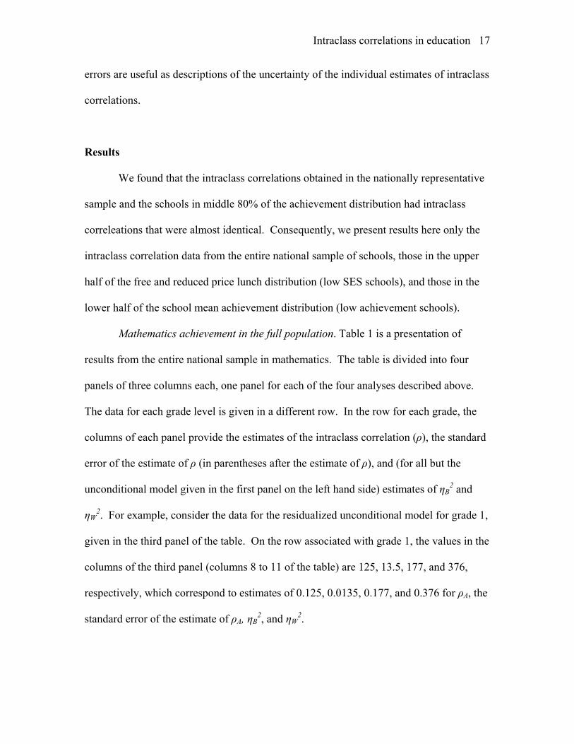
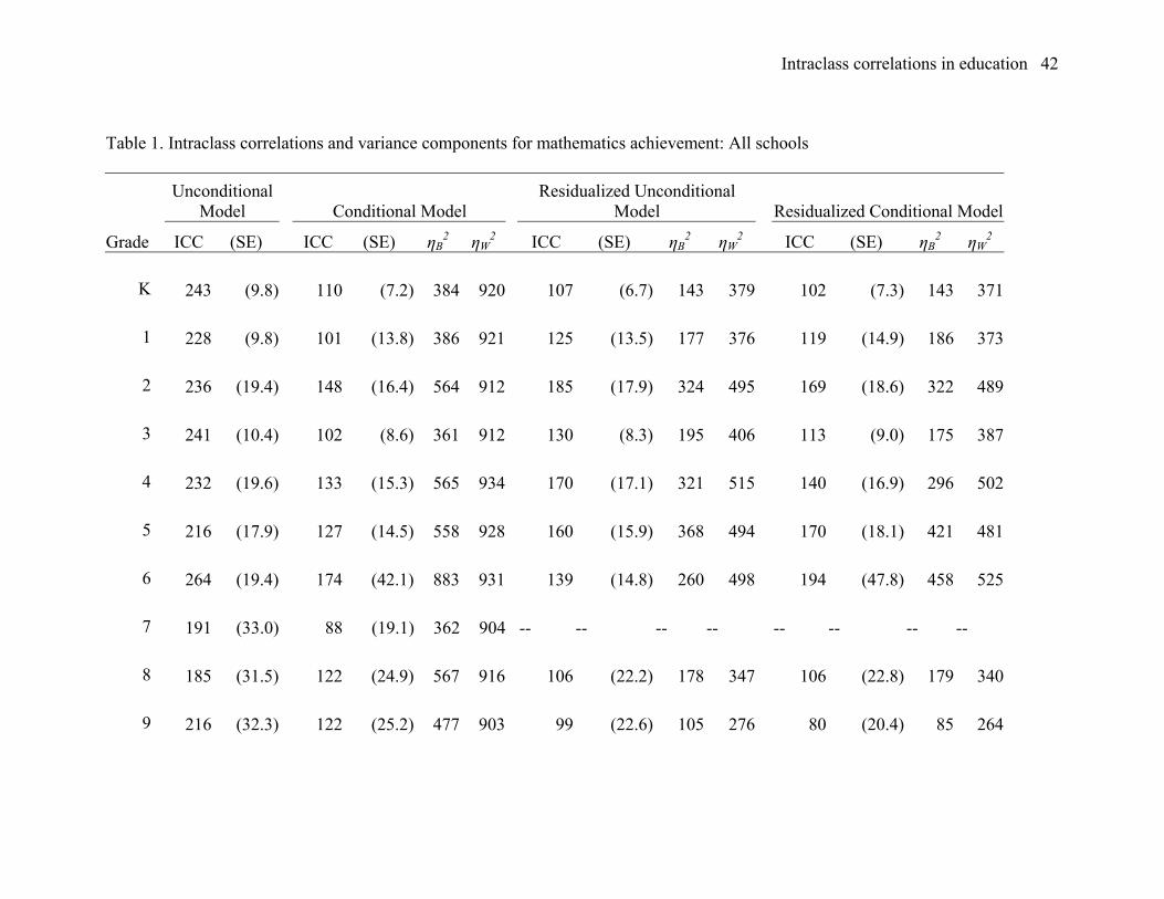
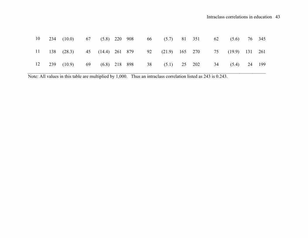
Mathematics achievement in the full population. Table 1 is a presentation of
results from the entire national sample in mathematics. The table is divided into four
panels of three columns each, one panel for each of the four analyses described above.
The data for each grade level is given in a different row. In the row for each grade, the
columns of each panel provide the estimates of the intraclass correlation (ρ), the standard
error of the estimate of ρ (in parentheses after the estimate of ρ), and (for all but the
unconditional model given in the first panel on the left hand side) estimates of ηB2 and
ηW2. For example, consider the data for the residualized unconditional model for grade 1,
given in the third panel of the table. On the row associated with grade 1, the values in the
columns of the third panel (columns 8 to 11 of the table) are 125, 13.5, 177, and 376,
respectively, which correspond to estimates of 0.125, 0.0135, 0.177, and 0.376 for ρA, the
standard error of the estimate of ρA, ηB2, and ηW
2.

Intraclass correlations in education 18
Although there is a tendency of the intraclass correlations to be larger at lower
grades, in general there are not large changes across adjacent grade levels. Few of these
differences exceed two standard errors of the difference. A notable exception is the
unadjusted intraclass correlation at grade 11, where the difference between grade 11 and
either of the adjacent grades is about three standard errors of the difference. None of the
differences between adjusted intraclass correlations in adjacent grades is a large as three
standard errors of the difference, but the values for grade 2 are somewhat higher (by over
two standard errors of the difference) and those for grade 3 somewhat lower than those of
adjacent grades.
The pattern of reduction of between and within-cluster (school) variances are
generally quite different in these models. Specifically, the conditional analyses typically
reduced the between cluster variance to one-half to one-quarter of its value in the
unconditional model (e.g., produced ηB2 from 0.5 to 0.25), but typically reduced within-
cluster variance by 10% or less (e.g., produced ηW2 values greater than 0.9). The
residualized analyses using pretest score as a covariate typically resulted in larger
reductions in between-cluster variance (e.g., produced ηB2 values from 0.3 to 0.1), but
typically also reduced within-cluster variance by a much larger amount than the
conditional model (e.g., produced ηW2 values from 0.25 to 0.5). Different patterns of
variance reduction have quite different implications for statistical power, even if they
correspond to the same adjusted intraclass correlation (see the section on power
computation in models with covariates).
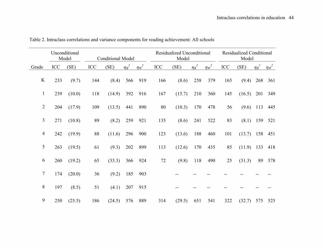
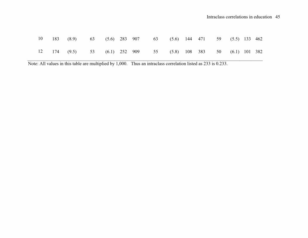
Reading achievement in the full population. Table 2 is a presentation of results
from the entire national sample in reading, organized in the same way as Table 1 which

Intraclass correlations in education 19
reported results for mathematics. The intraclass correlation and adjusted intraclass
correlation values in reading are generally quite similar to those in mathematics. As in
mathematics, there is a tendency of the intraclass correlations in reading to become
smaller at higher grades, but the changes across adjacent grade levels are often larger.
The results for grade 9 are particularly inconsistent with (having larger values of the
intraclass correlations than) the results from either grade 8 or grade 10. The results from
grade 2 are also somewhat different (having smaller values of the intraclass correlations
than) the results from either grade 1 or grade 3. Several of these differences exceed three
standard errors of the difference. Few of the other differences exceed two standard errors
of the difference.
There is less consistency in reading than in mathematics among the adjusted
intraclass correlations for the three models involving covariates. However the general
pattern of reduction in between- versus within-cluster variance was similar in reading and
in mathematics. That is, there was somewhat greater reduction in between-cluster
variance and much greater reduction in within-cluster variance in the residualized model
than in the conditional model.
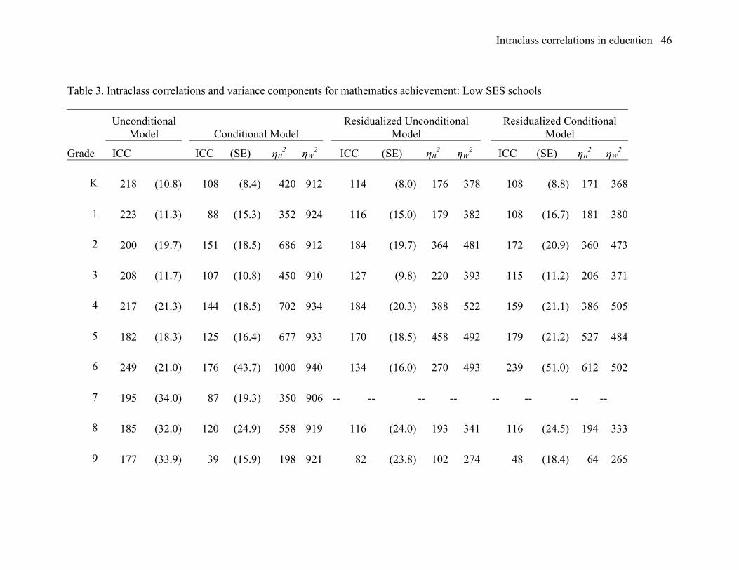
Mathematics achievement in low SES schools. Table 3 is a presentation of results
in mathematics computed for the schools in the bottom half of the school SES
distribution (operationalized by proportion of students eligible for free or reduced price
lunch). There appears to be a slight tendency for the intraclass correlation values in this
sample to be a bit smaller than those reported in Table 1 for the entire national population,
a tendency that does not hold for the conditional (adjusted) intraclass correlations. The
pattern of variation in the mathematics intraclass correlations and conditional intraclass
Intraclass correlations in education 20
correlations across regions, urbanicity of school setting, and regions crossed with
urbanicity in the low SES school sample was similar to that in all schools.
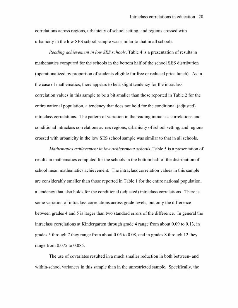
Reading achievement in low SES schools. Table 4 is a presentation of results in
mathematics computed for the schools in the bottom half of the school SES distribution
(operationalized by proportion of students eligible for free or reduced price lunch). As in
the case of mathematics, there appears to be a slight tendency for the intraclass
correlation values in this sample to be a bit smaller than those reported in Table 2 for the
entire national population, a tendency that does not hold for the conditional (adjusted)
intraclass correlations. The pattern of variation in the reading intraclass correlations and
conditional intraclass correlations across regions, urbanicity of school setting, and regions
crossed with urbanicity in the low SES school sample was similar to that in all schools.
Mathematics achievement in low achievement schools. Table 5 is a presentation of
results in mathematics computed for the schools in the bottom half of the distribution of
school mean mathematics achievement. The intraclass correlation values in this sample
are considerably smaller than those reported in Table 1 for the entire national population,
a tendency that also holds for the conditional (adjusted) intraclass correlations. There is
some variation of intraclass correlations across grade levels, but only the difference
between grades 4 and 5 is larger than two standard errors of the difference. In general the
intraclass correlations at Kindergarten through grade 4 range from about 0.09 to 0.13, in
grades 5 through 7 they range from about 0.05 to 0.08, and in grades 8 through 12 they
range from 0.075 to 0.085.
The use of covariates resulted in a much smaller reduction in both between- and
within-school variances in this sample than in the unrestricted sample. Specifically, the

Intraclass correlations in education 21
conditional analyses typically reduced the between-school variance to no less than one-
half of its value in the unconditional model (e.g., produced ηB2 from 0.5 to 0.8), but
typically reduced within-cluster variance by 5% or less (e.g., produced ηW2 values greater
than 0.95). The residualized analyses using pretest score as a covariate typically (but not
always) resulted in modestly larger reductions in between-cluster variance (e.g., produced
ηB2 values from 0.3 to 0.8), but typically reduced within-cluster variance by a larger
amount than the conditional model (e.g., produced ηW2 values from 0.5 to 0.8). Thus we
find that the intraclass correlation is smaller in this sample, but the explanatory power of
pretest and other covariates is also smaller. These two tendencies have opposite effects
on statistical power. The smaller intraclass correlation generally leads to larger statistical
power but the smaller explanatory power of covariates generally leads to larger statistical
power, one partially offsetting the effects of the other.
Reading achievement in low achievement schools. Table 6 is a presentation of
results in mathematics computed for the schools in the bottom half of the distribution of
school mean reading achievement. As in the case of mathematics, the intraclass
correlation values in this sample are considerably smaller than those reported in Table 2
for the entire national population, a tendency that also holds for the conditional (adjusted)
intraclass correlations.
There is some variation of intraclass correlations across grade levels. The
intraclass correlation in grade 9 is larger (by over three standard errors of the difference)
than that in either of the adjacent grades. Similarly the intraclass correlation in grade 1 is
more than two standard errors greater than that in Kindergarten, but less than two
standard errors of the difference from that in grade 2. None of the other differences

Intraclass correlations in education 22
between grades is this large in comparison to their uncertainty. In general the intraclass
correlations at grades Kindergarten through 4 range from about 0.10 to 0.14, in grades 5
through 8 they range from about 0.06 to 0.07, and in grades 10 through 12 they are about
0.05.
As in the case of mathematics, the use of covariates resulted in a much smaller
reduction in both between- and within-school variances in this sample than in the national
sample. Specifically, the conditional analyses typically reduced the between-school
variance to no less than one-half of its value in the unconditional model (e.g., produced
ηB2 from 0.5 to 0.8), but typically reduced within-cluster variance by 5% or less (e.g.,
produced ηW2 values greater than 0.95). The residualized analyses using pretest score as a
covariate typically (but not always) resulted in modestly larger reductions in between-
cluster variance (e.g., produced ηB2 values from 0.3 to 0.8), but typically reduced within-
cluster variance by a larger amount than the conditional model (e.g., produced ηW2 values
from 0.5 to 0.8). Thus we find, as in the case of mathematics, that the intraclass
correlation is smaller in this sample, but the explanatory power of pretest and other
covariates is also smaller, one of these differences partially offsetting the effects of the
other on statistical power.
Minimum Detectable Effect Sizes
One way to summarize the implications of these results for statistical power is to
use them to compute the smallest effect size for which a target design would have
adequate statistical power. This effect size is often called the minimum detectable effect
size (MDES), see Bloom (1995) and Bloom (2005). In computing the MDES values

Intraclass correlations in education 23
reported in this paper, we used the value 0.8 with a two-sided test at significance level
0.05 as the definition of adequate power. We considered designs with no covariates and
with pretest as a covariate at both the individual and group level. We considered both
reading and mathematics achievement as potential outcomes. Finally we considered a
balanced design with a sample of size of n = 60 per school with m = 10, 15, 20, 25, or 30
schools randomized to each treatment group.
Table 7 gives the minimum detectable effect sizes based on parameters given in
Tables 1 and 2 that were estimated from the full national sample. Perhaps the most
obvious finding is that the corresponding MDES values for mathematics and reading are
quite similar. With no covariates, the MDES values typically exceed 0.60 for m = 10 and
typically exceed 0.35 even for m = 30. However the use of pretest as a covariate reduces
the MDES values to less than 0.40 for m = 10 and 0.20 or less for m = 30. Although
there is no universally adequate standard for evaluating the importance of effect sizes,
applying Cohen’s (1977) widely used labels of 0.20 as small and 0.50 as medium would
imply that an experiment randomizing m = 10 schools to each treatment should be
adequate to detect effects of “medium” size and that an experiment randomizing m = 30
schools to each treatment should be adequate to detect effects of “small” size.
Table 8 gives the minimum detectable effect sizes based on parameters given in
Tables 3 and 4 that were estimated from the national sample of low SES schools. These
results are remarkably similar to those in Table 7.
Table 9 gives the minimum detectable effect sizes based on parameters given in
Tables 5 and 6 that were estimated from the national sample of schools in the lower half
of the achievement distribution. Because the unconditional intraclass correlations are

Intraclass correlations in education 24
lower, the MDES values for designs with no covariates are smaller. However because
the covariates are less effective in reducing between and with-school variance in this
sample, the MDES values with pretest as a covariate are not always smaller than in the
national sample of all schools. With no covariates, the MDES values typically less than
0.50 for m = 10 and less than 0.30 for m = 30. However the use of pretest as a covariate
typically reduces the MDES values to about 0.30 for m = 10 and 0.20 or less for m = 30.
Using the Results of this Paper to Compute Statistical Power
of Cluster Randomized Experiments
In this section, we illustrate the use of the results in this paper to compute the
statistical power of cluster randomized experiments. Consider the two treatment group
design with q (0 ≤ q < M – 2) group-level (cluster-level) covariates and p (0 ≤ p < N – q
– 2) individual-level covariates in the analysis. Note that we specifically include the
possibility that there are 0 (no) covariates at a given level. For example a design with p =
1 and q = 1 might arise, for example, if there was a pretest that was used as an individual-
level covariate and cluster means on the covariate were used as a group level covariate.
We assume also that the individual-level covariate has been centered about cluster means.
The structural model for Yijk, the kth observation in the jth cluster in the ith treatment might
be described in ANCOVA notation as
( )ijk Ai I ijk G ij A i j AijkY µ α γ= + + + + + +' 'θ x θ z ε ,
where µ is the grand mean, αAi is the covariate adjusted effect of the ith treatment, θI =
(θI1, …, θIp)’ is a vector of p individual-level covariate effects, θG = (θG1, …, θGq)’ is a

Intraclass correlations in education 25
vector of q group-level covariate effects, xij is a vector of p group (cluster) centered
individual-level covariate values for the jth cluster in the ith treatment, zij is a vector of q
group-level (cluster-level) covariate values for the jth cluster in the ith treatment, γ(i)j is the
random effect of cluster j within treatment i, and εAijk is the covariate adjusted within cell
residual. Here we assume that both of the random effects (clusters and the residual) are
normally distributed.
The analysis might be carried out either as an analysis of covariance with clusters
as a nested factor or by viewing the model as a hierarchical linear model and using
software for multilevel models such as HLM. In multilevel model notation, it would be
conventional to specify a level-one (individual-level) model as
0ijk j j ijk AijkY β ε= + +'β x ,
and a level-two (cluster-level) model for the intercept as
0 00 01 02j A i ijTREATMENT ζβ π π= + + +'π z Aj ,
where TREATMENTi is a dummy variable for the treatment group, while the covariate
slopes in βj would be treated as fixed effects (βj = θI), and ζAj is the random effect of the
jth cluster (a level-two residual). With the appropriate constraints on the ANCOVA
model (i.e., setting αAi = 0 for the control group and constraining the mean of the γA(i)j’s to
be 0), these two models are identical and there is a one to one correspondence between
the parameters and the random effects in the two models. That is, µ = π00, αAi = πA01, θG =
π02, θI = βj (for all j), γA(i)j = ζAj (with a suitable redefinition of the index j), and εAijk
identical in both models. The variance components associated with this analysis are σAW2
(the variance of the εAijk) and σAB2 (the variance of the ζj), where the A in the subscript
denotes that these variance components are adjusted for the covariate.

Intraclass correlations in education 26
The intraclass correlations. Note that if in the experiment, schools were sampled
at random, students were sampled at random within schools, and q = p = 0, then ρ =
σB2/[σB
2 + σW2] is exactly the intraclass correlation that would obtain in a survey that
sampled first schools and then students at random. Similarly, if there are covariates in
the experiment, schools were sampled at random, students were sampled at random
within schools, and q ≠ 0 or p ≠ 0, then ρA = σAB2/[σAB
2 + σAW2] is exactly the adjusted
intraclass correlation that would obtain in the analysis of the survey (with appropriate
covariates) that sampled first schools and then students at random.
Hypothesis Testing
The object of the statistical analysis is to test the statistical significance of the
intervention effect, that is, to test the hypothesis
H0: αA1 – αA2 = 0
or equivalently
H0: πA01 = 0.
The ANCOVA t-test statistic is
1 2( A AA
A
m Y YtS•• ••−
=) , (5)
where is as defined above,m 1AY •• and 2AY •• are the adjusted means, SA is the pooled within-
treatment-groups adjusted standard deviation of cluster means, and the subscript A is
used to connote that the means and standard deviation are adjusted for the covariates. The
F-test statistic from a one-way analysis of covariance using cluster means is of course
2ABA A
AC
MSFMS
= = t . (6)

Intraclass correlations in education 27
In this case MSAB = 21 2( A Anm Y Y•• ••− ) and MSAC = nSA
2, where SA is the pooled within-
treatment-groups standard deviation of the covariate adjusted cluster means (the standard
deviation of the level-two residuals). If the null hypothesis is true, the test statistic tA has
Student’s t-distribution with M – q – 2 degrees of freedom. Equivalently, the test statistic
FA has the central F-distribution with 1 degree of freedom in the numerator and M – q – 2
degrees of freedom in the denominator when the null hypothesis is true.
When the null hypothesis is false, the test statistic tA has for this analysis has a
noncentral t-distribution with M – q – 2 degrees of freedom and noncentrality parameter
[ ]
11 1 1 1
A1 A2 AA
AT A A
mn mnδλσ n ρ n ρ
−= =
+ − + −
( )( ) ( )
α α , (7)
where δA = (αA1 – αA2)/σAT.
Alternatively (and equivalently), the F-statistic has the noncentral F-distribution
with 1 degree of freedom in the numerator and M – q – 2 degrees of freedom in the
denominator and noncentrality parameter
2
2
( )[1 ( 1) ]
A1 A2A
AT A
mnωn ρ
α ασ
−=
+ −.
For the purposes of power computation, the expression (7) is not convenient,
because the minimum effect size of interest is likely to be known in units of the
unadjusted standard deviation rather than the adjusted standard deviation, that is we are
more likely to know δ = (α1 – α2)/σT rather than δA = (αA1 – αA2)/σAT . In a randomized
experiment, covariate adjustment should not affect the treatment effect parameter, so that
αA1 – αA2 = α1 – α2, but the covariate adjustment necessarily affects the standard deviation.
This is true even if the covariates operate at only one level of the design. Because

Intraclass correlations in education 28
2 2 2AT AB Aσ σ σ= + W , a covariate adjustment at the individual-level will affect σAT
2 via
σAW2 and a covariate adjustment at the cluster-level will affect σAT
2 through σAB2.
To express λA in terms of δ, we need only express σAT in terms of σT. A direct
derivation shows that
[ ]
2 2 2
2 2
( )( ) 11 ( 1) 1 ( 1)
B W B AA1 A2 TA
T AT A B W
mn mnσ n ρ n ρA
η η η ρα α σλ δσ η η⎛ ⎞ + −−
= =⎜ ⎟ + − + −⎝ ⎠. (8)
An alternative, but equivalent, expression of λA that is considerably more
revealing involves ηB2, ηW
2, and the unadjusted intraclass correlation ρ. This expression
is
( )2 2 2
1A
W B W
mnnη η ρ
λ δη
=+ −
. (9)
Note that the quantity [ηW2 + (nηB
2 – 1)ρ] is analogous to [1 + (n – 1)ρ], Kish’s design
effect. We see that [ηW2 + (nηB
2 – 1)ρ] reduces to [1 + (n – 1)ρ] in the analysis without
covariates (because ηW2 = ηB
2 = 1) and (9) reduces to the expression given, for example in
Blair and Higgins (1986) for the t-test conducted using cluster means as the unit of
analysis.
We illustrate the use of the t-statistic. The power of the one-tailed test at level α
is
p1 = 1 – H[c(α, M – q – 2), (M – q – 2), λA] (10)
where c(α, ν) is the level α one-tailed critical value of the t-distribution with ν degrees of
freedom [e.g., c(0.05,10) = 1.81], and H(x, ν, λ) is the cumulative distribution function of
the noncentral t-distribution with ν degrees of freedom and noncentrality parameter λ.
The power of the two-tailed test at level α is

Intraclass correlations in education 29
p2 = 1 – H[c(α/2, M – q – 2), (M – q – 2), λA] + H[–c(α/2, M – q – 2), (M – q – 2), λA] (11)
Using Power Tables and Power Calculation Software
Many tabulations (e.g., Cohen, 1977) and programs (e.g., Borenstein, Rothstein,
and Cohen, 2001) are available for computing statistical power from designs involving
simple random samples, but tables for computing power from the independent-groups t-
test are the most widely available. Following Cohen’s framework, such tables typically
provide power values based on sample sizes N1T and N2
T (often assumed to be equal for
simplicity) and effect size ∆T, where the superscript T indicates that these quantities are
what is used in the power tables. The calculations on which they are based translate the
sample sizes and effect size into degrees of freedom νT and noncentrality parameter λT in
order to compute statistical power. In the case of the two sample t-test they do so via
νT = N1T + N2
T – 2
and
T TNλ = ∆T ,
where
1 2
1 2
T TT
T T
N NNN N
=+
.
Tables like Cohen’s (or the corresponding software) can be used to compute the power of
the test used in the case of clustered sampling by judicious choice of sample sizes and
effect size. We have to enter the table with a configuration of sample sizes and a
synthetic effect size (here called the operational effect size) that will yield the appropriate
degrees of freedom and noncentrality parameter.

Intraclass correlations in education 30
If the actual numbers of clusters assigned are m1 and m2, then entering the power
table with sample sizes N1T = m1 – q and N2
T = m2 yields νT = (m1T + m2
T – 2) = M – q – 2,
the correct degrees of freedom for the test. Of course, many other combinations of
sample sizes will also yield the correct degrees of freedom as well and will yield
equivalent results as long as the operational effect size is modified in a corresponding
manner. The relevant operational effect size using our choice of degrees of freedom is
[ ] ( )
2 2 2
2 2 2 2 2
( ) 11 ( 1)
T B W B AT T
B W A W B W
mn mnN n ρ N nη η ρ
η η η ρδ δη η η
+ −∆ = =
+ − + −, (12)
where δ is the unadjusted effect size, ρ is the unadjusted intraclass correlation, and ηB2
and ηW2 are defined in (5) and (6) above. If the analysis makes a covariate adjustment at
the cluster level the ηB2 is the appropriate value given in the tables of this paper, but if the
analysis makes no covariate adjustment at the cluster level (that is q = 0), then ηB2 ≡ 1.
Similarly, if the analysis makes a covariate adjustment at the individual (within–cluster)
level the ηW2 is the appropriate value given in the tables of this paper, but if the analysis
makes no covariate adjustment at the individual level (that is if p = 0), then ηW2 ≡ 1.
Note that the value of ∆T given in (13) is appropriate because, when this is multiplied
by TN , it yields the noncentrality parameter λA given in (12). Using ρ or ρA, the cluster
sample size n, and the variance ratios ηB2 and ηW
2 to compute operational effect size
makes it possible to compute statistical power and sample size requirements for analyses
based on clustered samples using these tables and computer programs designed for the
two group t-test.
Example with No Covariates at Either Level

Intraclass correlations in education 31
Consider an experiment that will randomize m1 = m2 = 10 schools to receive an
intervention to improve mathematics achievement so that n = 20 students in each school
would be part of the experiment. There are no covariates at either individual or group
level so that p = q = 0 and ηW2 = ηB
2 = 1. The analysis will involve a two-tailed t-test with
significance level α = 0.05. Suppose that the smallest educationally significant effect size
for this intervention is assumed to be δ = 0.50. Suppose further that the schools were
chosen to attempt to be represent first graders nationally.
Entering Table 1 on the first row for grade 1 and the panel for the unconditional
model (columns 3 to 5) gives the intraclass correlation for first graders as ρ = 0.228.
Then the variance inflation factor is
1 + (20 – 1)(0.228) = 5.332,
so that the noncentrality parameter from (4) is
0.50 (10 / 2)20
2.1655.332
λ = = .
Using (6) and the noncentral t-distribution function, (for example the function NCDF.T in
SPSS), with M – 2 = 18 degrees of freedom, c(0.05/2, 18) = 2.101, and λ = 2.165, we
obtain a two-sided power of p2 = 1 – 0.467 + 0.000 = 0.53.
Alternatively, we could compute the power from tables of the power of the t-test
such as those given by Cohen (1977). To do so, we first compute the operational effect
size given in (8) as
0.50 20 0.9685.332
T∆ = = .
Cohen’s tables give the statistical power in terms of sample size (in each treatment group)
and effect size. Examining Cohen’s (1977) Table 2.3.5, we see that the operational effect

Intraclass correlations in education 32
size of 0.968 is between tabled effect sizes of 0.8 and 1.0. Entering the Table with
sample size N1T = N2
T = 10, we see that a power of 0.39 is tabulated for the effect size of
∆T = 0.80 and a power of 0.56 is tabulated for an effect size of ∆T = 1.00. Interpolating
between these two values we obtain a power of 0.53 for ∆T = 0.97.
Note that in this case (and many others) the operational effect size for the tests
based on clustered samples is larger than the actual effect size (in this case 0.97 versus
0.50). This does not mean that the power of the test for the design based on the clustered
sample is larger than that based on a simple random sample with the same total sample
size. The reason is that the test using the clustered sample has many fewer degrees of
freedom in the error term. For example, a test based on an effect size of ∆T = 0.50 and a
simple random sample of nm = (10)(20) = 200 in each group would have power
essentially 1.0.
Example with Pretest as a Covariate at Both Individual and Cluster Level
Consider an experiment that will randomize m1 = m2 = 10 schools to receive an
intervention to improve first grade reading achievement and that n = 20 students in each
school would be part of the experiment. An analysis of covariance will be used with
pretest as a covariate at both individual and school level (so that p = q = 1) using a two-
tailed test with significance level α = 0.05. Suppose that the smallest educationally
significant effect size for this intervention is δ = 0.25. Suppose further that the schools
were chosen to attempt to be representative of first graders nationally.
Entering Table 2 on the first row for grade 1 and the panel for the unconditional
model (columns 3 to 5) gives the intraclass correlation for first graders as ρ = 0.239.

Intraclass correlations in education 33
Entering Table 2 on the second row for grade 1 and the panel for the residualized
unconditional model (columns 9 to 11) gives the between- and within-school variance
ratios after covariate adjustment as ηB2 = 0.210 and ηW
2 = 0.360. Then the variance
inflation factor is
0.360 + [(20)(0.210) – 0.360](0.239) = 1.2778,
so that the noncentrality parameter from (15) is
0.25 (10 / 2)20
2.211.1.278Aλ = =
Using (17) and the noncentral t-distribution function, (for example the function NCDF.T
in SPSS), with M – 2 – 1 = 17 degrees of freedom, c(0.05/2, 17) = 2.110, and λA = 2.211,
we obtain a two-sided power of p2 = 1 – 0.450 + 0.000 = 0.55.
Alternatively, we could compute the power from tables of the power of the t-test
such as those given by Cohen (1977). Because there is q = 1 covariate at the school level
N1T = m1 – 1 = 10 – 1 = 9 and N2
T = m2 = 10. Because Cohen’s tables give the statistical
power in terms of equal sample sizes (in each treatment group), we will need to
interpolate between sample sizes N1T = N2
T = 9 and N1T = N2
T = 10. Here we compute
= (10 x 10)/(10 + 10) = 5. Note that the operational effect size depends on N1T and N2
T,
so we have to compute a different value of ∆T for each of the sample sizes between which
we will interpolate. For N1T = N2
T = 9, = (9 x 9)/(9 + 9) = 4.50 and the operational
effect size is
m
TN
(4.5)(20) 10.25 1.0435 1.2778
T∆ = = .
For N1T = N2
T = 10, = (10 x 10)/(10 + 10) = 5.0 and the operational effect size is TN

Intraclass correlations in education 34
(5)(20) 10.25 0.9895 1.2778
T∆ = = .
Examining Cohen’s (1977) Table 2.3.5 we see that the effect size ∆T = 1.04 is
between tabled values of effect size of 1.0 and 1.2. Entering the Table with sample size
N1T = N2
T = 9, we see that a power of 0.51 is tabulated for the effect size of ∆T = 1.0 and a
power of 0.67 is tabulated for an effect size of ∆T = 1.2. Interpolating between the two
power values (0.51 and 0.65) for N1T = N2
T = 9, we obtain a power of 0.54 for ∆T = 1.04.
This value (0.54) corresponds to the power associated with the effect size of δ = 0.25 and
a test based on 16 degrees of freedom.
Examining Cohen’s (1977) Table 2.3.5 again we also see that the effect size ∆T =
0.99 is between tabled values of effect size of 0.8 and 1.0. Entering the Table with
sample size N1T = N2
T = 10, we see that a power of 0.39 is tabulated for the effect size of
∆T = 0.80 and a power of 0.56 is tabulated for an effect size of ∆T = 1.00. Interpolating
between the two power values (0.39 and 0.56) for N1T = N2
T = 10, we obtain a power of
0.55 for ∆T = 0.99. This value (0.55) corresponds to the power associated with the effect
size of δ = 0.25 and a test based on 18 degrees of freedom.
To obtain the power associated with an effect size of δ = 0.25 and a test based on
17 degrees of freedom we must interpolate once again between these two values, we
obtain a power value for N1T = 9 and N2
T = 10 of p2 = 0.55.
It is worth noting that if no covariates had been used at either level of this analysis
(that is if p = q = 0 and therefore ηB2 = ηW
2 = 1), the power would have been 0.17. If the
pretest as a covariate had been used only at the individual level (that is if p = 1 and q = 0
and ηB2 = 1, but ηW
2 = 0.360), the power would have increased to 0.18. But if the pretest
had been used as a covariate only at the school level (that is if p = 0 and q = 1 and ηW2 = 1,

Intraclass correlations in education 35
but ηB2 = 0.210), the power would have increased to 0.43. This illustrates the fact that
covariates at the (group) cluster level can have far more impact on the power than
covariates at the individual level.
Conclusions
The values of intraclass correlations and variance components presented in this
paper provide some guidance for the selection of intraclass correlations for planning
cluster randomized experiments that have samples as diverse as the nation as a whole and
those using low SES schools. These values suggest somewhat larger values of the
intraclass correlation (roughly 0.15 to 0.25) may be appropriate than the 0.05 to 0.15
guidelines that have sometimes been used. The guideline of 0.05 to 0.15 is more
consistent with the values of covariate adjusted intraclass correlations we found.
In using these values, it is important to keep in mind that these analyses do not
separately estimate the between-district and between-state components of variance.
Therefore these two components of variance are included here as part of the between-
school variance. This is desirable if the values are to be used in connection with designs
that involve schools from several districts or states. However if the design involves
schools from only a single district or state, the estimates reported here may overestimate
the relevant intraclass correlations to some degree. Unfortunately, it is unclear just how
much of an impact this may have. There are also likely to be some impact on the
effectiveness of the covariates in explaining between- and within-school variation. It is
possible that the somewhat greater between-school variation leads to a larger intraclass

Intraclass correlations in education 36
correlation, but also a larger covariate effect so that these impacts partially cancel one
another in their effects on statistical power.
A more detailed compilation is available from the authors providing values for
regions of the country, settings with different levels of urbanicity, and regions crossed
with levels of urbanicity. However it is important to recognize that there may be a
tradeoff between bias (estimating exactly the right value of the intraclass correlation in a
particular context) and variance (the sampling uncertainty of that estimate). The variance
of the intraclass correlation estimate is driven primarily by the number of clusters (in this
case, schools). While intraclass correlations we computed in a particular region and
setting are more specific and therefore likely to have less bias as estimates of the
intraclass correlation in an experiment that is to be conducted within a particular region
and context, the sample size used to estimate the intraclass correlations is smaller and
thus the estimate is subject to greater sampling uncertainties. Our analyses suggest that,
while there is often statistically significant variation in intraclass correlations between
regions and settings, the magnitude of this variation is typically small. Thus it is not
completely clear whether more specific estimates are always better (more accurate) for
planning purposes.
Although we anticipate that the principal use of the results given in this paper will
be for planning randomized experiments in education that assign schools (rather than
individuals) to treatments, there are other potential applications. One involves the use of
information external to an experiment to adjust the degrees of freedom of significance
tests in designs involving group randomization, called the df* method by its originators
(see Murray, Hannan, and Baker, 1996). While the originators of this method caution

Intraclass correlations in education 37
that it is important that users should have good reasons to assume that any external
estimates used should estimate the same intraclass correlation as that in the experiment,
there may be situations in which data from this compilation meets that assumption.
Because they are based on relatively large samples, the intraclass correlation estimates
reported in this paper tend to have small standard errors. Consequently, if they are
thought to be appropriate for use in a particular df* computation, they should
substantially increase the degrees of freedom used in the test for treatment effects.
A second potential application is to evaluate whether the conclusions of statistical
analyses that incorrectly ignored clustering might have changed if those significance tests
had taken clustering into account. Hedges (in press a) has shown how to compute the
actual significance level of the usual t-statistic when it has been computed from clustered
samples (by incorrectly ignoring clustering). The computation of this actual significance
level depends on ρ. The values in this compilation provide some guidelines on values of
ρ that might be used for sensitivity analyses to see if a conclusion about the statistical
significance of a treatment effect might not have held if clustering had been taken into
account.
A third potential application involves the computation of standardized effect size
estimates and their standard errors in group randomized trials. There are several
approaches to the computation of effect size estimates in multilevel designs, but in some
cases, computation of estimates and the computation of standard errors requires
knowledge of ρ (see, Hedges, in press b). In cases where the report of the experiment
itself does not include information that can be used to compute an estimate of ρ, this
compilation may provide some idea of a range of plausible values to incorporate into

Intraclass correlations in education 38
sensitivity analyses used in connection with effect sizes from experiments that assign
schools to treatment.

Intraclass correlations in education 39
References
Blair, R. C. & Higgins, J. J. (1986). Comment on “Statistical power with group mean as
the unit of analysis.” Journal of Educational Statistics, 11, 161-169. Bloom, H. S. (1995). Minimum detectable effects: A simple way to report statistical
power of experimental designs. Evaluation Review, 19,547-556. Bloom, H. S. (2005). Randomizing groups to evaluate place-based programs. In H. S.
Bloom (Ed.) Learning morefrom social experiments: Evolving analytic approaches. New York: Russell Sage Foundation.
Bloom, H. S., Bos, J. M., & Lee, S. W. (1999). Using cluster random assignment to
measure program impacts: statistical implications for the evaluation of educational programs. Evaluation Review, 23, 445-469.
Bloom, H. S., Richburg-Hayes, L., & Black, A. R. (2005). Using covariates to improve
precision: Empirical guidelines for studies that randomize schools to measure the impacts of educational interventions. New York, NY: MDRC.
Borenstein, M., Rothstein, H., and Cohen, J. (2001). Power and precision. Teaneck, N.J.:
Biostat, Inc. Cohen, J. (1977). Statistical power analysis for the behavioral sciences (2nd Edition).
New York: Academic Press. Curtin, T. R., Ingels, S. J., Wu, S., & Heuer, R. (2002). User’s Manual: Nels:88 base-
year to fourth followup. Washington, DC: US National Center for Education Statistics.
Donner, A., Birkett, N., & Buck, C. (1981). Randomization by cluster. American Journal
of Epidemiology, 114, 906-914. Donner, A. & Klar, N. (2000). Design and analysis of cluster randomization trials in
health research. London: Arnold. Donner, A., and J. J. Koval. (1982). Design considerations in the estimation of intraclass
correlation. Annals of Human Genetics, 46, 271-77. Donner, A., and Wells, G. (1986). A comparison of confidence interval methods for the
intraclass correlation coefficient. Biometrics, 42, 401-12. Guilliford, M. C., Ukoumunne, O. C., & Chinn, S. (1999). Components of variance and
intraclass correlations for the design of community-based surveys and
Intraclass correlations in education 40
intervention studies. Data from the Health Survey for England 1994. American Journal of Epidemiology, 149, 876-883.
Hannan, P. J., Murray, D. M., Jacobs, D. R., & McGovern, P. G. (1994). Parameters to
aid in the design and analysis of community trials: Intraclass correlations from the Minnesota heart health program. Epidemiology, 5, 88-95.
Hedges, L. V. (1983). Combining independent estimators in research synthesis. British
Journal of Mathematical and Statistical Psychology, 36, 123-131. Hedges, L.V. (in press a). Correcting a significance test for clustering. Journal of
Educational and Behavioral Statistics. Hedges, L.V. (in press b). Effect sizes in cluster randomized designs. Journal of Educational
and Behavioral Statistics. Hopkins, K. D. (1982). The unit of analysis: Group means versus individual observations.
American Educational Research Journal, 19, 5-18. Kish, L. (1965). Survey sampling. New York: John Wiley. Klar, N. & Donner, A. (2001). Current and future challenges in the design and analysis of
cluster randomization trials. Statistics in Medicine, 20, 3729-3740. Kraemer. H. C. & Thiemann, s. (1987). How many subjects? Statistical power analysis in
research. Newbury Park, CA: Sage Publications. Lipsey, M. W. (1990). Design sensitivity: Statistical power analysis for experimental
research. Newbury Park, CA: Sage Publications. Mosteller, F. & Boruch, R. (Eds.) (2002). Evidence matters: Randomized trials in
education research. Washington, DC: Brookings Institution Press. Miller, J. D., Hoffer, T., Suchner, R. W., Brown, K. G., & Nelson, C. (1992). LSAY
Codebook. DeKalb, IL: Northern Illinois University. Murray, D. M. (1998). Design and analysis of group-randomized trials. New York:
Oxford University Press. Murray, D. M. & Blitstein, J. L. (2003). Methods to reduce the impact of intraclass
correlation in group-randomized trials, Evaluation Review, 27, 79-103. Murray, D. M., Hannan, P. J., & Baker, W. L. (1996). A Monte Carlo study of alternative
responses to intraclass correlation in community trials. Evaluation Review, 20, 313-337.

Intraclass correlations in education 41
Murray, D. M., Varnell, S. P., & Blitstein, J. L. (2004). Design and analysis of group-randomized trials: A review of recent methodological developments. American Journal of Public Health, 94, 423-432.
Myers, D. & Schirm, A. (1999). The impacts of upward bound: Final report for phase I
of the national evaluation. Washington, DC: Mathematica Policy Research. Puma, M. J., Karweit, N., Price, C., Riccuti, A., & Vaden-Kiernan, M. (1997). Prospects:
Final report on student outcomes, volume II: Technical report. Cambridge, MA: Abt Associates.
Raudenbush, S. W. (1997). Statistical analysis and optimal design for cluster randomized
experiments. Psychological Methods, 2, 173-185. Raudenbush, S. W. & Bryk, A. S. (2002). Hierarchical linear models. Thousand Oaks,
CA: Sage Publications. Ridgeway, J. E., Zawgewski, J. S., Hoover, M. N., & Lambdin, D. V. (2002). Student
attainment in connected mathematics curriculum. Pages 193-224 in S. L. Senk & D. R. Thompson (Eds.) Standards-based school mathematics curricula: What are they? What do students learn? Mahwah, NJ: Erlbaum.
Schochet, P. Z. (2005). Statistical power for random assignment evaluations of
educational programs. Princeton, NJ: Mathematica Policy Research. Snijders, T. & Bosker, J. (1993). Standard errors and sample sizes for two-level research.
Journal of Educational Statistics, 18, 237-259. Tourangeau, K. Brick, M, Le, T., Nord, C., West, J., Hausken, E. G. (2005). Early
childhood longitudinal study, Kindergarten class of 1998-99. Washington, DC: US National Center for Education Statistics.
Verma, V. & Lee, T. (1996). An analysis of sampling errors for demographic and health
surveys. International Statistical Review, 64, 265-294.
Intraclass correlations in education 42
Table 1. Intraclass correlations and variance components for mathematics achievement: All schools
Unconditional
Model Conditional ModelResidualized Unconditional
Model Residualized Conditional Model
Grade ICC (SE) ICC (SE) ηB2 ηW
2 ICC (SE) ηB2 ηW
2 ICC (SE) ηB2 ηW
2
K 243
(9.8) 110 (7.2) 384 920 107 (6.7) 143 379 102 (7.3) 143 371
1 228 (9.8) 101 (13.8) 386 921 125 (13.5) 177 376 119 (14.9) 186 373
2 236 (19.4) 148 (16.4) 564 912 185 (17.9) 324 495 169 (18.6) 322 489
3 241 (10.4) 102 (8.6) 361 912 130 (8.3) 195 406 113 (9.0) 175 387
4 232 (19.6) 133 (15.3) 565 934 170 (17.1) 321 515 140 (16.9) 296 502
5 216 (17.9) 127 (14.5) 558 928 160 (15.9) 368 494 170 (18.1) 421 481
6 264 (19.4) 174 (42.1) 883 931 139 (14.8) 260 498 194 (47.8) 458 525
7 191 (33.0) 88 (19.1) 362 904 --
--
--
--
--
--
--
--
8 185 (31.5) 122 (24.9) 567 916 106 (22.2) 178 347 106 (22.8) 179 340
9 216 (32.3) 122 (25.2) 477 903 99 (22.6) 105 276 80 (20.4) 85 264
Intraclass correlations in education 43
10
234 (10.0) 67 (5.8) 220 908 66 (5.7) 81 351 62 (5.6) 76 345
11
138 (28.3) 45 (14.4) 261 879 92 (21.9) 165 270 75 (19.9) 131 261
12 239 (10.9) 69 (6.8) 218 898 38 (5.1) 25 202 34 (5.4) 24 199
Note: All values in this table are multiplied by 1,000. Thus an intraclass correlation listed as 243 is 0.243.
Intraclass correlations in education 44
Table 2. Intraclass correlations and variance components for reading achievement: All schools
Unconditional
Model Conditional Model Residualized Unconditional
Model Residualized Conditional
Model
Grade ICC (SE) ICC (SE) ηB2 ηW
2 ICC (SE) ηB2 ηW
2 ICC (SE) ηB2 ηW
2
K 233
(9.7) 144
(8.4) 566
919
166 (8.6) 258
379
165
(9.4) 268
361
1 239
(10.0)
118
(14.9) 392
916
167 (15.7) 210
360
145
(16.5) 201
349
2 204
(17.9)
109
(13.5) 441
890
80 (10.3) 170
478
56 (9.6) 113
445
3
271
(10.8)
89 (8.2) 259
921
135 (8.6) 241
522
83 (8.1) 159
521
4
242
(19.9)
88 (11.6) 296
900
123 (13.6) 188
460
101
(13.7) 158
451
5 263
(19.5)
61 (9.3) 202
899
113 (12.6) 170
435
85 (11.9) 133
418
6 260
(19.2)
65 (33.3) 366
924
72 (9.8) 118
490
25 (31.3) 89
578
7 174
(20.0)
36 (9.2) 185
903
-- --
--
--
-- --
--
8
197
(8.5) 51 (4.1) 207
915
-- --
--
--
-- --
--
9
250
(25.5)
186
(24.5) 576
889
314 (29.5) 651
541
322
(32.7) 575
525
Intraclass correlations in education 45
10
183
(8.9) 63 (5.6) 283
907
63 (5.6) 144
471
59 (5.5) 133
462
12 174 (9.5) 53 (6.1) 252 909 55 (5.8) 108 383 50 (6.1) 101 382
Note: All values in this table are multiplied by 1,000. Thus an intraclass correlation listed as 233 is 0.233.
Intraclass correlations in education 46
Table 3. Intraclass correlations and variance components for mathematics achievement: Low SES schools
Unconditional
Model Conditional ModelResidualized Unconditional
Model Residualized Conditional
Model
Grade ICC ICC (SE) ηB2 ηW
2 ICC (SE) ηB2 ηW
2 ICC (SE) ηB2 ηW
2
K 218
(10.8) 108 (8.4) 420 912 114 (8.0) 176 378 108 (8.8) 171 368
1 223 (11.3) 88 (15.3) 352 924 116 (15.0) 179 382 108 (16.7) 181 380
2 200 (19.7) 151 (18.5) 686 912 184 (19.7) 364 481 172 (20.9) 360 473
3 208 (11.7) 107 (10.8) 450 910 127 (9.8) 220 393 115 (11.2) 206 371
4 217 (21.3) 144 (18.5) 702 934 184 (20.3) 388 522 159 (21.1) 386 505
5 182 (18.3) 125 (16.4) 677 933 170 (18.5) 458 492 179 (21.2) 527 484
6 249 (21.0) 176 (43.7) 1000 940 134 (16.0) 270 493 239 (51.0) 612 502
7 195 (34.0) 87 (19.3) 350 906 --
--
--
--
--
--
--
--
8 185 (32.0) 120 (24.9) 558 919 116 (24.0) 193 341 116 (24.5) 194 333
9 177 (33.9) 39 (15.9) 198 921 82 (23.8) 102 274 48 (18.4) 64 265

Intraclass correlations in education 47
10
174 (11.5) 67 (7.6) 316 908 63 (7.4) 113 355 60 (7.4) 108 349
11 134 (34.8) 58 (21.5) 331 869 126 (33.9) 239 266 111 (32.3) 179 248
12 172 (12.5) 65 (8.8) 324 896 37 (6.7) 38 200 41 (7.6) 45 195 Note: All values in this table are multiplied by 1,000. Thus an intraclass correlation listed as 218 is 0.218.

Intraclass correlations in education 48
Table 4. Intraclass correlations and variance components for reading achievement: Low SES schools
Unconditional
Model Conditional ModelResidualized Unconditional
Model Residualized Conditional
Model
Grade ICC (SE) ICC (SE) ηB2 ηW
2 ICC (SE) ηB2 ηW
2 ICC (SE) ηB2 ηW
2
K 215
(10.8) 144
(9.8) 617
910
168 (10.1) 307
397
166 (11.1) 314
377
1 227
(11.5) 118
(17.5) 383
919
152 (17.3) 196
366
145 (19.3) 199
357
2 181
(18.4) 119
(15.9) 533
891
66 (10.1) 155
484
50 (10.3) 108
449
3 223
(12.0) 98 (10.5) 355
908
123 (9.8) 267
495
85 (10.3) 197
493
4 214
(20.9) 96 (14.2) 385
896
138 (16.7) 253
471
113 (17.1) 217
467
5 230
(20.6) 61 (10.7) 246
905
123 (15.0) 222
440
89 (14.0) 165
420
6 221
(19.9) 59 (32.6) 500
920
70 (10.7) 137
494
23 (27.4) 125
576
7 173
(23.4) 52 (13.6) 230
908
-- -- -- -- -- -- -- --
8 137
(10.2) 57 (6.4) 361
905
--
-- --
--
--
-- --
--
9 236
(31.9) 131
(26.5) 410
897
213 (32.6) 412
538
231 (38.1) 363
524

Intraclass correlations in education 49
10 131
(9.9) 56 (7.0) 381
905
47 (6.6) 163
470
47 (6.7) 166
463
12 131 (11.0) 44 (7.6) 297 906 50 (7.4) 134 367 41 (7.6) 118 365
Note: All values in this table are multiplied by 1,000. Thus an intraclass correlation listed as 215 is 0.215.

Intraclass correlations in education 50
Table 5. Intraclass correlations and variance components for mathematics achievement: Low achievement schools
Unconditional
Model Conditional ModelResidualized
Unconditional Model Residualized Conditional
Model
Grade ICC (SE) ICC (SE) ηB2 ηW
2 ICC (SE) ηB2 ηW
2 ICC (SE) ηB2 ηW
2
K 113
(8.6) 44 (8.0) 347 959 73 (7.7) 382 612 64 (9.2) 329 625
1 89 (8.7) 53 (17.3) 556 969 85 (15.8) 506 568 68 (18.5) 459 594
2 111 (14.6) 67 (14.2) 804 982 92 (14.3) 480 641 88 (17.5) 635 675
3 102 (10.4) 50 (11.0) 503 976 77 (9.8) 411 554 69 (11.9) 411 553
4 134 (15.7) 81 (14.8) 864 989 127 (16.8) 709 796 101 (18.8) 815 826
5 59 (10.0) 41 (11.1) 811 981 80 (12.8) 838 767 75 (15.6) 888 784
6 82 (12.8) 78 (41.7) 1000 924 98 (14.6) 1000 771 147 (54.1) 1000 660
7 45 (14.6) 37 (13.8) 794 982 -- -- -- -- -- -- -- --
8 85 (22.7) 73 (21.5) 876 958 67 (19.8) 552 685 56 (18.9) 486 666
9 81 (23.8) 66 (22.6) 790 953 56 (20.7) 429 558 54 (21.3) 418 550

Intraclass correlations in education 51
10
76 (8.2) 50 (7.9) 641 972 65 (8.5) 622 752 65 (8.8) 641 736
11 81 (24.0) 42 (18.4) 531 930 85 (25.0) 525 502 72 (24.1) 466 484
12 80 (9.7) 51 (9.9) 626 962 42 (8.4) 234 443 50 (10.0) 288 448 Note: All values in this table are multiplied by 1,000. Thus an intraclass correlation listed as 113 is 0.113.

Intraclass correlations in education 52
Table 6. Intraclass correlations and variance components for reading achievement: Low achievement schools
Unconditional
Model Conditional ModelResidualized Unconditional
Model Residualized Conditional
Model
Grade ICC (SE) ICC (SE) ηB2 ηW
2 ICC (SE) ηB2 ηW
2 ICC (SE) ηB2 ηW
2
K
104 (8.5) 79 (9.4) 817 948 118 (9.5) 807 712 111 (11.3) 843 707
1 142 (10.3) 66 (18.4) 472 967 158 (19.7) 592 529 129 (22.3) 572 539
2 109 (14.3) 92 (16.1) 816 967 38 (9.2) 278 783 32 (11.9) 219 780
3 139 (11.4) 80 (12.3) 494 972 75 (10.0) 381 649 57 (12.0) 301 670
4 103 (13.4) 66 (13.3) 694 978 90 (13.9) 557 717 94 (18.1) 629 742
5 71 (11.0) 27 (9.4) 477 978 85 (13.2) 764 727 57 (13.9) 707 734
6 58 (10.7) 66 (39.3) 1000 966 56 (11.1) 734 794 25 (29.7) 395 855
7 63 (11.8) 76 (20.4) 954 968 -- -- -- -- -- -- -- --
8 70 (6.5) 44 (5.7) 636 978 -- -- -- -- -- -- -- --
9 154 (22.7) 221 (31.1) 987 964 216 (28.4) 1000 853 292 (36.2) 1000 873

Intraclass correlations in education 53
10
50 (7.2) 44 (7.7) 882 961 50 (7.9) 895 848 56 (8.4) 949 831
12 47 (8.4) 36 (9.1) 774 956 46 (8.5) 663 684 50 (9.9) 792 685 Note: All values in this table are multiplied by 1,000. Thus an intraclass correlation listed as 104 is 0.104.

Intraclass correlations in education 54
Table 7. Minimum detectable effect sizes with power 0.80 and n = 60 as a function of m: All schools Mathematics Achievement Reading Achievement Grade Covariates m = 10 m = 15 m = 20 m = 25 m = 30m = 10 m = 15 m = 20 m = 25 m = 30
K none 0.67 0.54 0.46 0.41 0.38 0.66 0.53 0.46 0.41 0.37
pretest
0.27
0.22
0.19
0.17
0.15
0.34
0.28
0.24
0.21
0.19
1 none 0.66 0.53 0.45 0.40 0.37 0.67 0.54 0.46 0.41 0.37 pretest
0.29
0.23
0.20
0.18
0.16
0.32
0.25
0.22
0.19
0.18
2 none 0.67 0.53 0.46 0.41 0.37 0.62 0.50 0.43 0.38 0.35 pretest
0.39
0.31
0.27
0.24
0.22
0.27
0.22
0.19
0.17
0.15
3 none 0.67 0.54 0.46 0.41 0.38 0.71 0.57 0.49 0.44 0.40 pretest
0.31
0.25
0.21
0.19
0.17
0.36
0.29
0.25
0.22
0.20
4 none 0.66 0.53 0.45 0.41 0.37 0.67 0.54 0.46 0.41 0.38 pretest
0.38
0.31
0.26
0.24
0.21
0.31
0.25
0.21
0.19
0.17
5 none 0.64 0.51 0.44 0.39 0.36 0.70 0.56 0.48 0.43 0.39 pretest
0.39
0.32
0.27
0.24
0.22
0.30
0.24
0.21
0.19
0.17
6 none 0.70 0.56 0.48 0.43 0.39 0.70 0.56 0.48 0.43 0.39 pretest
0.37
0.30
0.25
0.23
0.21
0.26
0.21
0.18
0.16
0.15
7 none 0.60 0.48 0.42 0.37 0.34 0.58 0.46 0.40 0.36 0.32

Intraclass correlations in education 55
pretest
-- -- -- -- -- --
--
--
--
--
8 none 0.60 0.48 0.41 0.37 0.33 0.61 0.49 0.42
0.38 0.34 pretest
0.26
0.21
0.18
0.16
0.15
--
--
--
--
--
9 none 0.64 0.51 0.44 0.39 0.36 0.68 0.55 0.47 0.42 0.38 pretest
0.22
0.18
0.15
0.14
0.12
0.55
0.44
0.38
0.34
0.31
10 none 0.66 0.53 0.46 0.41 0.37 0.59 0.47 0.41 0.36 0.33 pretest
0.21
0.17
0.14
0.13
0.12
0.25
0.20
0.17
0.15
0.14
11 none 0.52 0.42 0.36 0.32 0.29 -- -- -- -- -- pretest
0.22
0.18
0.15
0.14
0.13
--
--
--
--
--
12 none 0.67 0.54 0.46 0.41 0.37 0.58 0.46 0.40 0.36 0.32 pretest 0.13 0.10 0.09 0.08 0.07 0.21 0.17 0.15 0.13 0.12
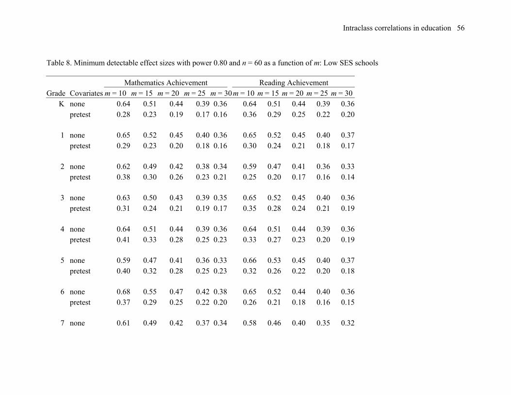
Intraclass correlations in education 56
Table 8. Minimum detectable effect sizes with power 0.80 and n = 60 as a function of m: Low SES schools Mathematics Achievement Reading Achievement Grade Covariates m = 10 m = 15 m = 20 m = 25 m = 30m = 10 m = 15 m = 20 m = 25 m = 30
K none 0.64 0.51 0.44 0.39 0.36 0.64 0.51 0.44 0.39 0.36
pretest
0.28
0.23
0.19
0.17
0.16
0.36
0.29
0.25
0.22
0.20
1 none 0.65 0.52 0.45 0.40 0.36 0.65 0.52 0.45 0.40 0.37 pretest
0.29
0.23
0.20
0.18
0.16
0.30
0.24
0.21
0.18
0.17
2 none 0.62 0.49 0.42 0.38 0.34 0.59 0.47 0.41 0.36 0.33 pretest
0.38
0.30
0.26
0.23
0.21
0.25
0.20
0.17
0.16
0.14
3 none 0.63 0.50 0.43 0.39 0.35 0.65 0.52 0.45 0.40 0.36 pretest
0.31
0.24
0.21
0.19
0.17
0.35
0.28
0.24
0.21
0.19
4 none 0.64 0.51 0.44 0.39 0.36 0.64 0.51 0.44 0.39 0.36 pretest
0.41
0.33
0.28
0.25
0.23
0.33
0.27
0.23
0.20
0.19
5 none 0.59 0.47 0.41 0.36 0.33 0.66 0.53 0.45 0.40 0.37 pretest
0.40
0.32
0.28
0.25
0.23
0.32
0.26
0.22
0.20
0.18
6 none 0.68 0.55 0.47 0.42 0.38 0.65 0.52 0.44 0.40 0.36 pretest
0.37
0.29
0.25
0.22
0.20
0.26
0.21
0.18
0.16
0.15
7 none 0.61 0.49 0.42 0.37 0.34 0.58 0.46 0.40 0.35 0.32

Intraclass correlations in education 57
pretest
-- -- -- -- -- --
--
--
--
--
8 none 0.60 0.48 0.41 0.37 0.33 0.52 0.42 0.36
0.32 0.29 pretest
0.27
0.22
0.19
0.17
0.15
--
--
--
--
--
9 none 0.58 0.47 0.40 0.36 0.33 0.67 0.53 0.46 0.41 0.37 pretest
0.20
0.16
0.14
0.12
0.11
0.43
0.35
0.30
0.27
0.24
10 none 0.58 0.46 0.40 0.36 0.32 0.51 0.41 0.35 0.31 0.29 pretest
0.21
0.17
0.15
0.13
0.12
0.23
0.18
0.16
0.14
0.13
11 none 0.52 0.41 0.36 0.32 0.29 -- -- -- -- -- pretest
0.26
0.21
0.18
0.16
0.14
--
--
--
--
--
12 none 0.58 0.46 0.40 0.35 0.32 0.51 0.41 0.35 0.31 0.29 pretest 0.13 0.11 0.09 0.08 0.08 0.21 0.17 0.14 0.13 0.12

Intraclass correlations in education 58
Table 9. Minimum detectable effect sizes with power 0.80 and n = 60 as a function of m: Low achievement schools Mathematics Achievement Reading Achievement Grade Covariates m = 10 m = 15 m = 20 m = 25 m = 30 m = 10 m = 15 m = 20 m = 25 m = 30
K none 0.48 0.38 0.33 0.29 0.27 0.46 0.37 0.32 0.28 0.26
pretest
0.31
0.25
0.21
0.19
0.17
0.41
0.33
0.28
0.25
0.23
1 none 0.43 0.35 0.30 0.27 0.24 0.53 0.42 0.36 0.32 0.30 pretest
0.31
0.25
0.22
0.19
0.18
0.41
0.33
0.28
0.25
0.23
2 none 0.47 0.38 0.33 0.29 0.27 0.47 0.38 0.32 0.29 0.26 pretest
0.34
0.27
0.23
0.21
0.19
0.28
0.22
0.19
0.17
0.16
3 none 0.46 0.37 0.32 0.28 0.26 0.52 0.42 0.36 0.32 0.29 pretest
0.30
0.24
0.21
0.19
0.17
0.34
0.27
0.23
0.21
0.19
4 none 0.52 0.41 0.36 0.32 0.29 0.46 0.37 0.32 0.28 0.26 pretest
0.44
0.35
0.30
0.27
0.25
0.35
0.28
0.24
0.22
0.20
5 none 0.37 0.29 0.25 0.23 0.21 0.39 0.32 0.27 0.24 0.22 pretest
0.33
0.27
0.23
0.21
0.19
0.35
0.28
0.24
0.21
0.19
6 none 0.42 0.34 0.29 0.26 0.23 0.36 0.29 0.25 0.22 0.20 pretest
0.41
0.33
0.28
0.25
0.23
0.32
0.25
0.22
0.19
0.18
7 none 0.33 0.27 0.23 0.20 0.19 0.38 0.3 0.26 0.23 0.21

Intraclass correlations in education 59
pretest
-- -- -- -- -- -- -- -- -- --
8 none 0.42 0.34 0.29 0.26 0.24 0.39 0.31 0.27 0.24 0.22 pretest
0.32
0.26
0.22
0.20
0.18
-- -- -- -- --
9 none 0.42 0.33 0.29 0.26 0.23 0.55 0.44 0.38 0.34 0.31 pretest
0.28
0.23
0.19
0.17
0.16
0.55
0.44
0.38
0.33
0.30
10 none 0.41 0.33 0.28 0.25 0.23 0.34 0.28 0.24 0.21 0.19 pretest
0.33
0.26
0.23
0.20
0.18
0.33
0.26
0.22
0.20
0.18
11 none 0.42 0.33 0.29 0.26 0.23 -- -- -- -- -- pretest
0.30
0.24
0.21
0.19
0.17
--
--
--
--
--
12 none 0.41 0.33 0.29 0.25 0.23 0.34 0.27 0.23 0.21 0.19 pretest 0.22 0.17 0.15 0.13 0.12 0.28 0.22 0.19 0.17 0.16