cs6463 1

Interprocedural Analysisand AbstractInterpretation

cs6463 2

Outline Interprocedural analysis

control-flow graph MVP: “Meet” over Valid Paths Making context explicit

Context based on call-strings Context based on assumption sets

Abstract interpretation

cs6463 3

Control-flow graph for a wholeprogram At each function definition proc p(x)

Create two special CFG nodes: init(p) and final(p)

Build CFG for the function body Use init(p) as the function entry node Connect every return node to final(p)

At each function call to p(x) with Split the original function call into two stmts

Enter p(x) (before making the call) and exit p(x) (after the call exits)

Connect enter p(x) ->init(p), final(p) -> exit p(x) Connect enter p(x) -> exit p(x) to allow the flow of extra context info

Three kinds of CFG edges Intra-procedural: internal control-flow within a procedure Procedure calls: from enter p(x) to init(p) Procedure returns: from final(p) to exit p(x)

cs6463 4

Interprocedural CFG Example

Problem: matching between function calls andreturns

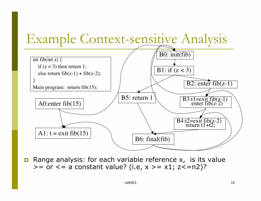
int fib(int z) { if (z < 3) then return 1; else return fib(z-1) + fib(z-2);}Main program: return fib(15);

B0: init(fib)

B6: final(fib)

B1: if (z < 3)

B5: return 1

B2: enter fib(z-1)

B3:t1=exit fib(z-1) enter fib(z-2)

B4:t2=exit fib(z-2) return t1+t2;

A0:enter fib(15)

A1: t = exit fib(15)

cs6463 5

Extending monotone frameworks Monotone frameworks consists of

A complete lattice (L,≤) that satisfies the Ascending ChainCondition

A set F of monotone transfer functions from L to L that contains the identity function and is closed under function composition

Transfer functions for procedure definitions For simplicity, both init(p) and final(p) have identity transfer

functions Transfer functions for procedure calls

For procedure entry: assign values to formal parameters For procedure exit: assign return values to outside

cs6463 6

Problem: calling context upon return

Matching between function calls and returns Calculating solutions on non-existing paths could seriously

detriment precision E.g. enter fib(z-2) -> init(fib) -> … -> exit fib(z-1) -> …

int fib(int z) { if (z < 3) then return 1; else return fib(z-1) + fib(z-2);}Main program: return fib(15);

B0: init(fib)

B6: final(fib)

B1: if (z < 3)

B5: return 1

B2: enter fib(z-1)

B3:t1=exit fib(z-1) enter fib(z-2)

B4:t2=exit fib(z-2) return t1+t2;

A0:enter fib(15)

A1: t = exit fib(15)

cs6463 7

MVP: “Meet” over Valid Paths Problem: matching procedure entries and exits

(function calls and returns) A complete path must

Have proper nesting of procedure entries and exits A procedure always return to the point immediately after

it is called

A valid path must Start at the entry node of the main program All the procedure exits match the corresponding entries Some procedures may be entered but not yet exited

The MVP solution At each program point t, the solution for t is

MVP(t) = Λ { sol(p) : p is a valid path to t }

cs6463 8

Making Context Explicit Context sensitive analysis

Maintain separate solutions for different callers of afunction

Extending the monotone framework Starting point (context-insensitive)

A complete lattice (L,≤) that satisfies the Ascending Chain Condition L = Power(D) where D is the domain of each solution

A set F of monotone transfer functions from L to L Extension

L = Power( D * C), where C includes all calling contexts F = L -> L, a separate sub-solution is calculated for each

calling context F (procedure entry) : attach caller info. to incoming solution F (procedure exit): match caller info, eliminate solution for

invalid paths

cs6463 9

Different Kinds of Context Call strings --- contexts based on control flow

Remember a list of procedure calls leading to the currentprogram point

Call strings of unbounded length --- remember all thepreceding calls

Call strings of bounded length (k) --- remember only thelast k calls

Assumption sets --- contexts based on data flow Assumption sets

Use the solution before entering proc p(x) as callingcontext (e.g., each context makes distinct presumptionsabout values of function parameters)

Large vs. small assumption sets How large is the context: use the entire solution or pick a

single constraint from the solution

cs6463 10

Example Context-sensitive Analysis

Range analysis: for each variable reference x, is its value>= or <= a constant value? (i.e, x >= x1; z<=n2)?

int fib(int z) { if (z < 3) then return 1; else return fib(z-1) + fib(z-2);}Main program: return fib(15);

B0: init(fib)

B6: final(fib)

B1: if (z < 3)

B5: return 1

B2: enter fib(z-1)

B3:t1=exit fib(z-1) enter fib(z-2)

B4:t2=exit fib(z-2) return t1+t2;

A0:enter fib(15)

A1: t = exit fib(15)

cs6463 11

Example Range Analysis

(none,t=?)

(A0,z=15,fib=?)(B2/B3,z=any,fib=1)

(B2/B3,z<=2)

(A0,z=15,t1/t2=?)(B2/B3,z>=3,t1/t2=?)

(A0,z=15,t1=?)(B2/B3,z>=3,t1=?)

(A0,z=15) (B2/B3,z>=3)

(A0,z=15) (B2/B3,z=?)

(A0,z=15) (B2/B3,z=?)

(none)

(none,t>=1)(none,t >=1)(none,t=?)A1

(A0,z=15,fib>=1)(B2/B3,z=any,fib>=1)

(A0,z=15,fib>=1)(B2/B3,z=any,fib>=1)

(none,z/fib=?)

B6

(B2,z=2) (B3,z<=2)(B2,z=2) (B3,z<=2)(none,z=?)

B5

(A0,z=15,t1/t2>=1)(B2/B3,z>=3,t1/t2>=1)

(A0,z=15,t1/t2=1)(B2/B3,z>=3,t1/t2=1)

(none,z/t1/t2=?)

B4

(A0,z=15,t1>=1)(B2/B3,z>=3,t1>=1)

(A0,z=15,t1=1)(B2/B3,z>=3,t1=1)

(none,z/t1=?)

B3

(A0,z=15)(B2/B3,z>=3)

(A0,z=15)(B2/B3,z>=3)

(none,z=?)

B2

(A0,z=15)(B2,z>=2)(B3,z>=1)

(A0,z=15)(B2,z>=2)(B3,z>=1)

(none,z=?)

B1

(A0,z=15)(B2,z>=2)(B3,z>=1)

(A0,z=15)(B2,z>=2)(B3,z>=1)

(none,z=?)

B0

(none)(none)(none)A0

Variables: x,z, t1, t2, fib, t; Contexts: A0, B2, B3,none;Domain: Variables * (<=n, =n, >=n,?,any)

cs6463 12

Foundations of AbstractInterpretation Definition from Wikipedia

abstract interpretation is a theory of sound approximation ofthe semantics of computer programs. It can be viewed as apartial execution of a computer program without performingall the calculations.

Outline Monotone frameworks

A complete lattice (L,≤) that satisfies the Ascending Chain Condition A set F of monotone transfer functions from L to L that

contains the identity function and is closed under function composition

Galois connections, closures,and Moore families Soundness and completeness of operations on abstract data Soundness and completeness of execution trace computation

cs6463 13

Galois Connections Two complete lattices

C: the “concrete” (execution) data The execution of the entire program Infinite and impossible to model precisely

A: the “abstract” (execution) data Properties (abstractions) of the “concrete” data The solution space (domain) of static program analysis

For complete lattices C and A, a Galois connection is A pair of monotonic functions, α : C->A, γ : A -> C For all a ∈ A and c ∈ C: c ≤ γ (α(c)) and α(γ (a)) ≤ a Is Written as C<α,γ>A

C A

cs6463 14

Galois Connections (2) γ and α are inverse maps of each

other’s image For all c∈γ(A),c=γ(α(c)); for all

a∈α(C),a=α(γ(a)) The maps α are

“homomorphism” mappingsbetween C and A

Galois connections are closedunder Composition, product, and so

on Each instruction performs an

action f: C->C Can use α and γ to define an

abstract transfer function f#:A->A for each f: C->C

{1}

{1,3,5,7…}

{1,3,5}

{}

{2,4}{1,2,3}

{1,2,3,4,…}

oddeven

none

all

α

γ

cs6463 15

Closure Maps For C<α,γ>A, it is common that

A ⊆ C. This means A embedsinto C as a sub-lattice A’s elements name

distinguished sets in C A closure map defines the

embedding of A within C. Definition: ρ:C->C is a closure

map if it is Monotonic: ∀ c1,c2 ∈ C, c1 ≤

c2 => ρ(c1) ≤ ρ(c2); extensive: ∀ c ∈ C, c ≤ ρ(c); idempotent: ∀ c ∈ C, ρ(ρ(c))=

ρ(c) (i.e. ρ * ρ = ρ)

{1}

{1,3,5,7…}

{1,3,5}

{}

{2,4}{1,2,3}

{1,2,3,4,…}

oddeven

none

allα

γ

1) Every Galois connection,C<α,γ>A defines a closuremap α • γ;

2) Every closure map, ρ:C->C,defines the Galoisconnection, C<ρ,id>ρ(C).

cs6463 16

Moore Families Given C, can we define a closure map on it by choosing some

elements of C? Yes, if the elements we select are closed under greatest-lower-bounds

(meet) operation That is, the new set of elements forms a complete lattice

Definition: M ⊆ C is a Moore family iff for all S ⊆ M, (^S) ∈ M. We can define a closure map as ρ(c)=^{c’ ∈ M | c ≤ c’}. That is, we map each element in C to the closest abstraction

(approximation) in M For each closure map, ρ:C->C, its image, ρ(C), is a Moore family.

Given C, we can define an abstract interpretation by selecting some M⊆ C that is a Moore family

cs6463 17

Closed Binary Relations Often the solution of an analysis is a power set of its domain

The Galois connection can be written as Power(D)<α,γ>A Given unordered set D and complete lattice A, it is natural to relate

the elements in D to those in A by a binary relation, R ⊆ D * A, s.t. (d,a) ∈ R (or d R a, d |=R a) means “d has property a”. Example: D=Int, A={none,neg,pos,zero,nonneg,nonpos,any}.

Then 2 R nonneg, 2 R pos, and 2 R any. The adjoint function, γ : A->Power(D),can be defined as

γ(a) = {d ∈ D | d R a}. E.g., γ (nonneg)={0,1,2,...}. If R defines a Galois collection, then γ(A) defines a Moore family.

Proposition: R⊆D*A defines a Galois connection between(Power(D), A) iff R is U-closed: c R a and a ≤ a’ imply c R a’; R is G-closed: c R ^ {a | c R a }

cs6463 18

Concrete and Abstract Operations Now that we know how to model a solution space via

abstraction function α : C -> A, We must model concrete computation steps, f:C->C, by abstract

computation steps, f#:A -> A. Example: we have concrete domain, Nat, and concrete

operation, succ: Nat -> Nat, defined as succ(n)=n+1. abstract domain, Parity = {any, even, odd, none}. abstract operation, succ#:Parity -> Parity, defined as

succ#(even)=odd, succ#(odd)=even, succ#(any)=any,succ#(none)=none,

succ# must be consistent (sound) with respect to succ: if n Rn a, then succ(n) Rn succ#(a), where Rn ⊆ Nat * Parity relates numbers to their parities (e.g., 2 Rn

even, 5 Rn odd, etc.).

cs6463 19

Sound Approximation Given

Galois connection C<α,γ>A and functions f : C->C and f#:A-> A,

f# is a sound approximation of f iff For all c ∈ C, α(f(c)) ≤ f#(α(c)) For all a ∈ A, f(γ(a)) ≤ γ(f#(a))

That is, α defines a “semi-homomorphism” with respectto f and f#

c α(c)

f(c) α(f(c)) ≤ f#(α(c))

α

αf f#

cs6463 20

Sound Approximation Example Given

Galois connection Power(Nat)<α,γ>Parity and Concrete transfer function succ : Nat->Nat, succ(S) = { n + 1 | n ∈ S } Abstract transfer function succ#: Parity -> Parity, succ#(even)=odd, succ#(odd)=even succ#(any)=any, succ#(none)=none

succ# is a sound approximation of succ For all c ∈ Nat, α(succ(c)) = succ#(α(c))

{2,6} even

{3,7} odd

α

αsucc succ#

cs6463 21

Synthesizing f# from f Given C<α,γ>A, and function f : C->C, the most precise

f#:A->A that is sound with respect to f is f# best (a) = α (f (γ (a)))

Proposition: f# is sound with respect to f iff For all a ∈ A, f# best(a) ≤ f#(a) Of course, f#best has a mathematical definition—not an

algorithmic one—f#best might not be finitely computable! Parity example continued:

succ#best(even)= α (succ (γ (even))) = α (succ {2n | n≥0 }) ) = α({2n+1 | n≥0}) = odd

Question: what about other operators on Nat, e.g., *, / ?

cs6463 22

Completeness of Approximation(skip)Given C<α,γ>A, and function f : C->C, Function f#: A->A is sound with respect to f iff

For all c ∈ C, α (f (c)) ≤ f# ( α(c)) For all a ∈ A, f(γ(a)) ≤ γ(f#(a))

Function f#: A->A is forwards(γ) complete with respect to f iff For all a ∈ A, f(γ(a)) = γ(f#(a)) That is, γ(A) is closed under f : f(γ(A))⊆ γ(A)

Function f#: A->A is backwards(α) complete with respect to f iff For all c ∈ C, α (f (c)) = f# (α(c)) That is, α partitions C into equivalence classes: α(c)= α(c’) impliesα(f(c))=α(f(c’))

For an f# to be (forwards or backwards) complete, it must equalf#best=α (f (γ (a))) The structure of C<α,γ>A and f: C->C determines whether f# is complete.

cs6463 23

Transfer Functions andComputation steps Each program transition from program point pi to pj has

an associated transfer function, fij:C->C (or f#ij:A-> A),which describes the associated computation. This defines a computation step of the form, (pi,s) -> (pj,fij(s))

Example: Assignment p0:x=x+1;p1:··· has the transfer function f01(<…x:n…>) = <…x:n+1…> For multiple transitions in conditionals, attach a transfer function

to each possible transition (branch) to “filter” the data that arrivesat a program point.

e.g. p0: cases x≤y: p1:y=y-x; y≤x: p2:x=x-y; end

fp1(s) = if s[x] ≤ s[y] then s else bot; (filter out s unless s[x] ≤ s[y]) fp2(s) = if s[y] ≤ s[x] then s else bot; (filter out s unless s[y] ≤ s[x])

cs6463 24

Execution Traces An execution trace is a (possibly infinite) sequence,

(p0,s0)->(p1,s1)->···->(pj,sj)-> ···,s.t. for all i≥0: (pi,si) -> psucc(i),fi,succ(i)(si) No si equals bot

P0: while (x != 1) {P1: if Even(x)P2: x = x div2;P3: else x = 3*x + 1;}P5: exit;

Two concrete traces((pi,v) means (pi,x=v)):

p0,4p1,4p2,4p0,2p1,2p2,2p0,1p4,1

p0,6p1,6p2,6p0,3p1,3p2,3p0,10p4,1···

cs6463 25

Using Approximation to buildabstract traces

Each concrete transition, (pi,s)-> (pj,fij(s)), is reproduced by acorresponding abstract transition, (pi,a)->(pj,f#ij(a)), where s∈ γ(a)

The traces embedded in the abstract trace tree “cover” (simulate)the concrete traces

1. Each concretetransition is generatedby an fij;

2. Each abstract transitionis generated by thecorresponding f#ij.

Abstract over approximating trace:p0,evenp1,even

p4,oddp1,any

p3,odd

p2,even p0,any

cs6463 26

Shape Analysis Goal

To obtain a finite representation of the memorystorage

The analysis result can be used for Detection of pointer aliasing Detection of sharing between structures Software development tools

Detection of pointer errors, e.g. dereferences of nil-pointers Program verification

E.g.,reverse transforms a non-cyclic list to a non-cyclic list

cs6463 27

The Concrete Solution Space Model the memory (stack and heap)

Storage of local variables Stack = Var -> (Value ∪ Loc)

Map each local variable into a value or a unique location The heap storage

Heap = (Loc * Sel) -> (Value ∪ Loc)Map pairs of locations and selectors to values or locations

Model the operational semantics of programs Program state: State = ProgramPoint * Stack * Heap Example: (p1, (x:3,y:Ly), ( (Ly,val):5)) is a program state Each statement modifies Stack and Heap of the previous state

Stmt: State -> State

cs6463 28

Building Abstract Domains Given an unordered set, D, of concrete data values, we might ask,

“What are the properties about D that I wish to calculate? Can I relate these properties a ∈ A, to elements d ∈ D via a UG-closed

binary relation, R: D*A? Given a set, A, and a binary relation, R: D * A

Define γ: A->Power(D) as γ(a) = {d ∈ D | d R a} Define partial ordering on A: a ≤ a’ iff γ(a) ≤ γ(a’)

If there are distinct a and a’ such that γ(a)=γ(a’), then merge them to force U-closure

Ensure that γ(A) is a Moore family by adding greatest-lower-boundelements to A as needed.

This forces G-closure Use the existing machinery to define the Galois connection between

Power(D) and A

cs6463 29

Abstracting the Program State Build a binary relation, Rd: Data*AbsData

Rv: Value -> AbsValue ; Rl: Loc -> AbsLoc May ignore the values of non-pointer variables.

Build induced Galois connection, Power(Data)<α,γ>AbsData, we can Build Galois connections that abstract the concrete data <xi : vi> Rs <xi : ai> iff vi Rd ai Example: <x:3, y:4> Rs <x:any, y:any> A program point is abstracted to itself: p Rp p, the abstract domain of program points is ProgramPoint ∪ {top, bot} (to

make it a complete lattice) Finally, we can relate each concrete state to an abstract one: (p,s) Rs (p’,s’) iff p = p’ and s Rs s’

cs6463 30

Shape Graphs Shape analysis uses a shape graph to abstract the

memory storage Graph nodes denote a finite number of abstract locations:

Aloc = {Nx | Nx is pointed to by a set of local variables} ∪ Nφ Nx : the node represents all concrete Locations referred to by variables

in x Nφ : abstract summary location (all the other locations)

Each graph node abstracts a distinctive set of concrete Locations If variables x and y may be aliased, they must share a single graph

node A graph edge sel connect nodes n1 and n2 if n2 is pointed to by

n1.sel

N{x}

N{y}

N{z}

Nφ

x

yznext

next next

cs6463 31

Abstraction of Program States Abstraction of memory storage

Abstract Stack AbsStack = Var -> ALoc

Map each pointer variable into a unique abstract location (a shape graph node) Abstract heap

AbsHeap = (ALoc * Sel) -> (ALoc)Mapping pairs of abs locations and selectors to abs locations

Sharing information IS : ALoc -> { yes, no} For each abstract location in the shape graph, is it shared by pointers in the

heap? If IS(Nx) = yes, then Nx must have an incoming edge from Nφ or have more

than one incoming edges Transfer functions: P(AbsState) -> P(AbsState)

Program state: AbsState=ProgramPoint * AbsStack * AbsHeap * IS Each statement modifies mappings in the previous state

cs6463 32

Transfer functions(1) x = nil

F (S,H,IS) = (S’,H’,IS’) where (S’,H’,IS’) is obtained from (S,H,IS) by Removing x from all mappings (killing all previous info. about x)

Merging all Nφ nodes

Nv

N{x} Nwx

sel1

sel2

Nφ Nv

Nw

sel1

sel2

Nφ

(S,H,IS) (S’,H’,IS’)

cs6463 33

Transfer functions(2) x = y

F (S,H,IS) = (S’,H’,IS’) where (S’,H’,IS’) is obtained by modifying mappings for x to be

identical to those for y

Nv

N{y,..} Nwy

sel1

sel2

N{x,…}

(S,H,IS) (S’,H’,IS’)

xNv

N{x,y,.}

Nwy

sel1

sel2

N{…}x

cs6463 34

Transfer functions(3) x = y.sel

Remove the old binding for x Establish a new binding for x to be the same as y.sel

If there is no abstract location defined for y Error: dereference a null pointer

If there is an abstract location Ny s.t. S[y] = Ny, but there is noabstract location for (Ny,sel)

Error dereference a non-existing field If there exist abstract locations Ny and Nz s.t. S[y] = Ny and

H[Ny,sel] = Nz. Modify the mappings so that x points to Nz If Nz = Nφ, create a new node N{x} for x --- may need to create

multiple shape graphs to cover different cases Other transfer functions

E.g. x.sel = y; x.sel = nil; allocate(x);