Interpreting the variability of CO2 columns over North ...

HAL Id: hal-00304101https://hal.archives-ouvertes.fr/hal-00304101

Submitted on 16 Apr 2008

HAL is a multi-disciplinary open accessarchive for the deposit and dissemination of sci-entific research documents, whether they are pub-lished or not. The documents may come fromteaching and research institutions in France orabroad, or from public or private research centers.

L’archive ouverte pluridisciplinaire HAL, estdestinée au dépôt et à la diffusion de documentsscientifiques de niveau recherche, publiés ou non,émanant des établissements d’enseignement et derecherche français ou étrangers, des laboratoirespublics ou privés.

Interpreting the variability of CO2 columns over NorthAmerica using a chemistry transport model: application

to SCIAMACHY dataP. I. Palmer, M. P. Barkley, P. S. Monks

To cite this version:P. I. Palmer, M. P. Barkley, P. S. Monks. Interpreting the variability of CO2 columns over NorthAmerica using a chemistry transport model: application to SCIAMACHY data. Atmospheric Chem-istry and Physics Discussions, European Geosciences Union, 2008, 8 (2), pp.7339-7371. hal-00304101

https://hal.archives-ouvertes.fr/hal-00304101

https://hal.archives-ouvertes.fr

ACPD

8, 7339–7371, 2008

Interpreting column

CO2 Data

P. I. Palmer et al.

Title Page

Abstract Introduction

Conclusions References

Tables Figures

Back Close

Full Screen / Esc

Printer-friendly Version

Interactive Discussion

Atmos. Chem. Phys. Discuss., 8, 7339–7371, 2008

www.atmos-chem-phys-discuss.net/8/7339/2008/

© Author(s) 2008. This work is distributed under

the Creative Commons Attribution 3.0 License.

AtmosphericChemistry

and PhysicsDiscussions

Interpreting the variability of CO2 columns

over North America using a chemistry

transport model: application to

SCIAMACHY data

P. I. Palmer1, M. P. Barkley

1, and P. S. Monks

2

1School of GeoSciences, University of Edinburgh, UK

2Department of Chemistry, University of Leicester, UK

Received: 18 February 2008 – Accepted: 25 March 2008 – Published: 16 April 2008

Correspondence to: P. I. Palmer ([email protected])

Published by Copernicus Publications on behalf of the European Geosciences Union.

7339

http://www.atmos-chem-phys-discuss.net

http://www.atmos-chem-phys-discuss.net/8/7339/2008/acpd-8-7339-2008-print.pdf

http://www.atmos-chem-phys-discuss.net/8/7339/2008/acpd-8-7339-2008-discussion.html

http://creativecommons.org/licenses/by/3.0/

ACPD

8, 7339–7371, 2008

Interpreting column

CO2 Data

P. I. Palmer et al.

Title Page



Tables Figures

Back Close

Full Screen / Esc



Abstract

We use the GEOS-Chem chemistry transport model to interpret variability of CO2

columns and associated column-averaged volume mixing ratios (CVMRs) observed

by the SCIAMACHY satellite instrument during the 2003 North American growing sea-

son, accounting for the instrument averaging kernel. Model and observed columns,5

largely determined by surface topography, averaged on a 2×2.5

grid, are in excellent

agreement (model bias=3%, r>0.9), as expected. Model and observed CVMRs, de-

termined by scaling column CO2 by surface pressure data, are on average within 3%

but are only weakly correlated, reflecting a large positive model bias (10–15 ppmv) at

50–70N during midsummer at the peak of biospheric uptake. GEOS-Chem generally10

reproduces the magnitude and seasonal cycle of observed CO2 surface VMRs across

North America. During midsummer we find that model CVMRs and surface VMRs

converge, reflecting the instrument vertical sensitivity and the strong influence of the

land biosphere on lower tropospheric CO2 columns. We use model tagged tracers to

show that local fluxes largely determine CVMR variability over North America, with the15

largest individual CVMR contributions (1.1%) from the land biosphere. Fuel sources

are relatively constant while biomass burning make a significant contribution only dur-

ing midsummer. We also show that non-local sources contribute significantly to total

CVMRs over North America, with the boreal Asian land biosphere contributing close

to 1% in midsummer at high latitudes. We used the monthly-mean Jacobian matrix for20

North America to illustrate that: 1) North American CVMRs represent a superposition

of many weak flux signatures, but differences in flux distributions should permit inde-

pendent flux estimation; and 2) the atmospheric e-folding lifetimes for many of these

flux signatures are 3–4 months, beyond which time they are too well-mixed to interpret.

7340





ACPD

8, 7339–7371, 2008

Interpreting column

CO2 Data

P. I. Palmer et al.

Title Page



Tables Figures

Back Close

Full Screen / Esc



1 Introduction

The importance of the natural carbon cycle in understanding climate is well established

(IPCC, 2007). A better quantitative understanding of natural sources and sinks of car-

bon dioxide (CO2), in particular, is crucial if CO2 mitigation and sequestration activities

relying on these natural fluxes are to work effectively. Estimation of sources and sinks5

of CO2 using inverted atmospheric transport models to interpret atmospheric concen-

tration data has been generally effective but has had varied success in the tropics

where there is relatively little data (Gurney et al., 2002). Previous inversion studies

have used surface concentration data (Bousquet et al., 1999), representative of spa-

tial scales of the order of 1000 km by virtue of their location; aircraft concentration data10

(Palmer et al., 2006; Stephens et al., 2007) representative of spatial scales of the order

of 10–100 s km, and generally only available during intensive campaign periods; and

concentrations from tall towers (Chen et al., 2007), representative of spatial scales of

the order of <1–10 s km.

New CO2 column data from low-Earth orbit space-borne sensors (e.g., the Scan-15

ning Imaging Absorption Spectrometer for Atmospheric Chartography (SCIAMACHY)

(Bovensmann et al., 1999), the Orbiting Carbon Observatory (OCO) (Crisp et al., 2004;

Miller et al., 2007), and the Greenhouse Observating SATellite (GOSAT) (Hamazaki

et al., 2004)), measuring in the near-infrared (NIR), are sensitive to changes in CO2 in

the lower troposphere and therefore provide potentially useful data with which to esti-20

mate surface fluxes of CO2 (Chevallier et al., 2007). One of the main advantages of

space-borne sensors is their repeated global coverage, facilitating measurements, for

example, over remote tropical ecosystems that are currently poorly characterized by

in situ data. SCIAMACHY CO2 data, in particular, are representative of a 60 km×30 km

spatial footprint, comparable with the horizontal resolution of current generation atmo-25

spheric transport models; upcoming instruments will have better horizontal resolution.

At the time of writing, SCIAMACHY is the only space-borne sensor in orbit that mea-

sures CO2 columns sensitive to the lower troposphere. To date there have been very

7341





ACPD

8, 7339–7371, 2008

Interpreting column

CO2 Data

P. I. Palmer et al.

Title Page



Tables Figures

Back Close

Full Screen / Esc



few model studies of SCIAMACHY CO2 column data, which have provided only qualita-

tive comparisons (Buchwitz et al., 2005, 2007; Barkley et al., 2006c). In this paper, we

use the GEOS-Chem global 3-D chemistry transport model (CTM) to interpret the vari-

ability in CO2 columns from SCIAMACHY over North America during the 2003 growing

season. We focus on North America because of the extensive multi-platform measure-5

ment programme which can be used to help evaluate SCIAMACHY via the CTM.

A number of studies have illustrated that the precision and accuracy of measured

CO2 columns is critical to their success in better quantifying the carbon cycle. The

temporal and spatial variations in column data are much less than those in surface

concentration measurements (Olsen and Randerson, 2004). Inversions of synthetic10

data have shown that CO2 columns have to be retrieved with a precision of less than

1% over a 8×10

grid if they are to improve upon the existing ground-based network

used for source/sink estimation (Rayner and O’Brien, 2001). Consequently, unchar-

acterized systematic biases will compromise this ability (Miller et al., 2007). Use of

column CO2 has the benefit of effectively reducing the potential model bias introduced15

by inaccurate descriptions of vertical mixing (Olsen and Randerson, 2004). Nonethe-

less, recent work has highlighted the requirement of using accurate, synoptic-scale

atmospheric transport to interpret CO2 column data in order to minimize errors asso-

ciated with spatial sampling, particularly over geographical regions with active weather

systems (Corbin et al., 2008). The vertically integrated CO2 column abundance rep-20

resents the sum of an age-spectrum of airmasses. Young airmasses (defined in this

paper as <3 months), still bearing the signatures of surface fluxes, are subject to at-

mospheric dilution processes that eventually render these signatures indistinguishable

from the global background whose variability is determined by atmospheric transport.

In this paper we show that variability in space-borne CO2 columns over one region is25

determined by both national and international surface flux signatures (local biosphere

fluxes that reach 1.1% of the column-averaged volume mixing ratio, CVMR, generally

represent the largest signals) that can be used to estimate flux strengths via inverse

model calculations. We also emphasize that accounting for the vertical sensitivity of

7342





ACPD

8, 7339–7371, 2008

Interpreting column

CO2 Data

P. I. Palmer et al.

Title Page



Tables Figures

Back Close

Full Screen / Esc



the satellite instrument can, in some instances, enhance surface flux signatures.

Section 2 briefly describes the SCIAMACHY retrievals of CO2 used in this work and

presents CO2 distributions over North America. Section 3 describes the GEOS-Chem

CTM used for this study and presents a brief model evaluation using surface CO2

data over North America from the GLOBALVIEW network (GLOBALVIEW-CO2, 2006).5

Section 4 critically examines the comparison between model and SCIAMACHY CO2

columns and CVMRs. In Sect. 5 we use the model to estimate which land-based

fluxes determine the continental-scale variability of CVMRs over North America during

the growing season, and look in detail at two contrasting sites over North America. In

Sect. 6 we discuss how CVMRs data could be used to infer source and sink distribu-10

tions. We conclude the paper in Sect. 5.

2 SCIAMACHY CO2 data

SCIAMACHY is a nadir and limb-viewing UV/Vis/NIR solar backscatter instrument

aboard the ENVISAT satellite, launched in 2002 (Bovensmann et al., 1999). It mea-

sures from 240 to 2380 nm, with a resolution of 0.2–1.4 nm depending on the channel.15

ENVISAT is in a near-polar sun-synchronous orbit crossing the equator at about 10:00

local solar time in the descending node, achieving full longitudinal global coverage at

the equator within six days. SCIAMACHY makes measurements in an alternating nadir

and limb sequence. We use the nadir measurements that have a horizontal resolution

of 60×30 km2

(across × along track).20

We include here only a short description of the retrieval of SCIAMACHY CO2

and refer the reader to dedicated retrieval studies (Buchwitz et al., 2000; Barkley

et al., 2006a). CO2 columns are retrieved in the 1561.03–1585.39 nm wavelength win-

dow using the Full Spectral Initiation (FSI) (Barkley et al., 2006a) Weighting Func-

tion Modified Differential Optical Absorption Spectroscopy (WFM-DOAS) (Buchwitz25

et al., 2000). The mean fitting uncertainty of these columns is typically 1–4% (0.8–

3.2×1020

molec cm−2

based on a fitted column of 8×1021

molec cm−2

), which is largely

7343





ACPD

8, 7339–7371, 2008

Interpreting column

CO2 Data

P. I. Palmer et al.

Title Page



Tables Figures

Back Close

Full Screen / Esc



attributable to poor characterization of the atmospheric state (e.g., aerosols, cirrus

clouds) (Barkley et al., 2006a). Cloudy scenes are diagnosed using the SCIAMACHY

polarization measurement devices using a cloud algorithm developed by Krijger et al.

(2005), as described by Barkley et al. (2006a), and excluded from subsequent analy-

ses. We also exclude back scans, observations with solar zenith angles >75

(Barkley5

et al., 2006a), and observations over ocean due to very low surface albedo. We use

only observations with a retrieval error of <5% and within a range of 340–400 ppmv (to

adequately constrain the light path). Previous studies have extensively evaluated FSI

CO2 data against independent measurements over the Northern Hemisphere. Com-

parisons between SCIAMACHY CO2 and ground-based Fourier Transform Spectrom-10

eters (FTS) and a CTM show a negative bias of 2–4% in the absolute CVMRs mag-

nitudes. Strong correlations between SCIAMACHY CO2 anomalies and aircraft and

ground-based data imply that SCIAMACHY can track lower troposphere variability on

at least monthly timescales, and has the potential to monitor changes in CO2 (Barkley

et al., 2006b, c, 2007). At this time, several retrieval issues (e.g., aerosol contamina-15

tion) need to be resolved before the data are characterized sufficiently well for inverse

modelling.

Figure 1 shows monthly mean CO2 columns (molec cm−2

) over North America dur-

ing the 2003 growing season (here defined as April–September) averaged over the

GEOS-Chem 2×2.5

grid (Sect. 3). Observed columns represent the vertical integral20

of atmospheric CO2 weighted by the instrument averaging kernel that describes the

instrument sensitivity to changes in the vertical profile of CO2. As we show later in

Sect. 3 SCIAMACHY has most sensitivity to CO2 in the lower troposphere (Barkley

et al., 2006c). The average number of individual scenes that fall into a North American

2×2.5

grid box is between 25 and 50, depending on month; this effectively reduces25

the random error by approximately an order of magnitude. Outside the growing season

spatial coverage at high latitudes is reduced by seasonally varying solar zenith angle

and persistent cloud cover. Retrieved columns range from 6 to 8×1021

molec cm−2

with

the largest values during Springtime over the Northeast and the smallest values gener-

7344





ACPD

8, 7339–7371, 2008

Interpreting column

CO2 Data

P. I. Palmer et al.

Title Page



Tables Figures

Back Close

Full Screen / Esc



ally later in the summer. The spatial distribution of CO2 columns is determined largely

by surface topography, with the Rockies mountain range introducing an apparent lon-

gitudinal gradient across North America.

To remove artefacts introduced by surface elevation we normalize retrieved CO2

columns using the nearest 6-hourly 1.125×1.125

ECMWF model surface pressure5

(Barkley et al., 2006c) to derive a CVMR. As we discuss in Sect. 4 there is signif-

icantly less agreement between model and observed values of CVMR than column

abundances. Figure 2 shows monthly mean SCIAMACHY CO2 CVMRs from April

to September 2003 over North America. Values range from 350 to 390 ppmv with a

15–20 ppmv peak-to-peak seasonal cycle over regions with a strong biospheric sig-10

nal, consistent with previous studies (Olsen and Randerson, 2004). Other studies of

SCIAMACHY CO2 data have used O2 columns to normalize retrieved CO2 columns, to

derive a dry air CVMR, (Buchwitz et al., 2007). Using O2 instead of surface pressure

will partially cancel effects of aerosols and clouds on the light path. However, at the

time of writing the general efficacy of this approach is not well quantified owing to dif-15

ferences between the radiative transfer and subsequent averaging kernels of the CO2

and O2 spectral fitting windows. Future satellite missions (e.g., OCO and GOSAT) also

plan to use O2 to normalize derived CO2 columns.

3 The GEOS-Chem forward model of CO2: description and evaluation

We use the GEOS-Chem global 3-D chemistry transport model (v7-03-06) to calculate20

column concentrations of CO2 from prescribed surface CO2 fluxes described in this

section. We used the model with a horizontal resolution of 2×2.5

, with 30 vertical

levels (derived from the native 48 levels) ranging from the surface to the mesosphere,

20 of which are below 12 km. The model is driven by GEOS-4 assimilated meteorology

data from the Global Modeling and Assimilation Office Global Circulation Model based25

at NASA Goddard. The 3-D meteorological data is updated every six hours, and the

mixing depths and surface fields are updated every three hours. The CO2 simulation

7345





ACPD

8, 7339–7371, 2008

Interpreting column

CO2 Data

P. I. Palmer et al.

Title Page



Tables Figures

Back Close

Full Screen / Esc



is based on Suntharalingam et al. (2004) and Palmer et al. (2006); here, we provide a

description of modifications to these previous studies.

3.1 CO2 flux inventories

Table 1 reports the regional monthly mean estimates of CO2 fluxes from fuel combus-

tion (sum of fossil fuel and biofuel), biomass burning, and the land biosphere used5

in GEOS-Chem. Gridded fossil fuel emission distributions are representative of 1995

(Suntharalingam et al., 2004) which we have scaled to 2003 values using regional bud-

get estimates for the top 20 emitting countries in 2003 from the Carbon Dioxide Informa-

tion Analysis Center (Marland et al., 2007), including sources from fossil fuel burning,

gas flaring, and cement production. On a global scale the sum of these sources has in-10

creased by 14% relative to 1995 values. Biofuel emission estimates, taken from Yevich

and Logan (2003), represent climatological values. This source of CO2 is generally

less than 1% of the total fuel source for North America and western Europe but repre-

sents up to 18% of the total fuel source for Asia. In many regions, particularly Asia, the

distributions of fossil and bio-fuel emissions overlap significantly so we lump these fuel15

source together (FL). Monthly biomass burning (BB) emission estimates are taken from

the second version of the Global Fire Emission Database (GFEDv2) for 2003 (van der

Werf et al., 2006). These data are derived from ground-based and satellite observa-

tions and should describe well the burning distributions. Monthly mean air-sea fluxes of

CO2 are taken from Takahashi et al. (1999). As we show later the observed variability20

in SCIAMACHY data is determined largely by continental fluxes so we do not discuss

further the role of ocean exchange in this study. We use daily mean land biosphere

(BS) fluxes from the CASA model for 2001 (Randerson et al., 1997), in the absence

of corresponding fluxes for 2003. Year-to-year variability of CASA monthly mean land

biosphere CO2 fluxes is small (<10%) so our approach should not introduce significant25

error. We do not explicitly account for the contribution of fuel combustion CO2 from the

oxidation of reduced carbon species (Suntharalingam et al., 2005) as they make only

a small contribution to the CO2 column.

7346





ACPD

8, 7339–7371, 2008

Interpreting column

CO2 Data

P. I. Palmer et al.

Title Page



Tables Figures

Back Close

Full Screen / Esc



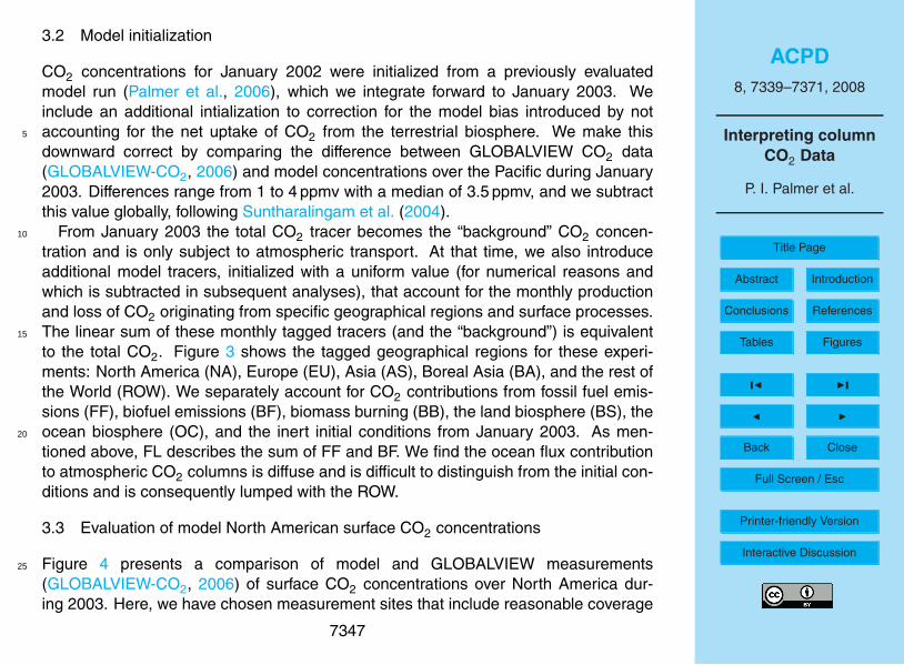
3.2 Model initialization

CO2 concentrations for January 2002 were initialized from a previously evaluated

model run (Palmer et al., 2006), which we integrate forward to January 2003. We

include an additional intialization to correction for the model bias introduced by not

accounting for the net uptake of CO2 from the terrestrial biosphere. We make this5

downward correct by comparing the difference between GLOBALVIEW CO2 data

(GLOBALVIEW-CO2, 2006) and model concentrations over the Pacific during January

2003. Differences range from 1 to 4 ppmv with a median of 3.5 ppmv, and we subtract

this value globally, following Suntharalingam et al. (2004).

From January 2003 the total CO2 tracer becomes the “background” CO2 concen-10

tration and is only subject to atmospheric transport. At that time, we also introduce

additional model tracers, initialized with a uniform value (for numerical reasons and

which is subtracted in subsequent analyses), that account for the monthly production

and loss of CO2 originating from specific geographical regions and surface processes.

The linear sum of these monthly tagged tracers (and the “background”) is equivalent15

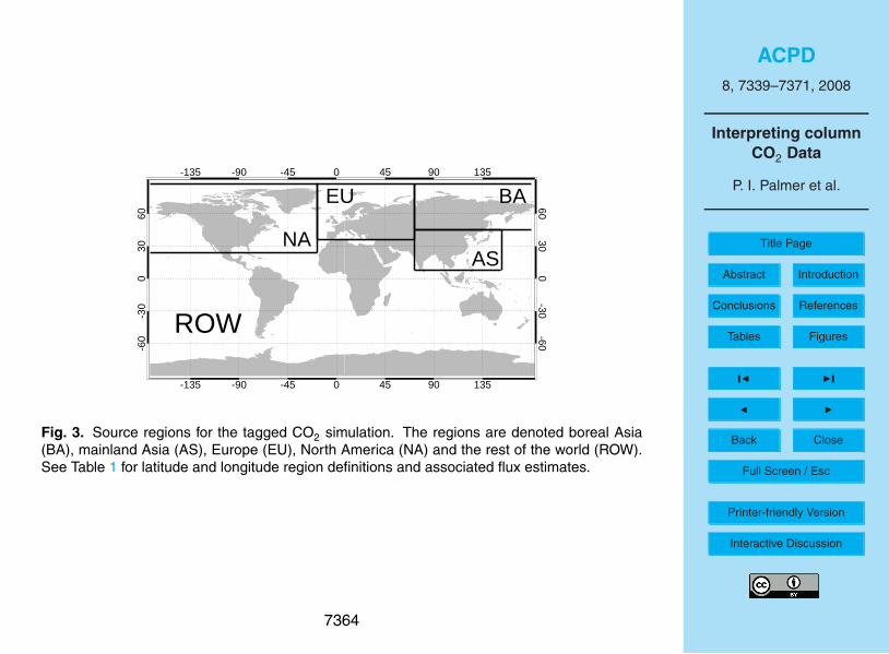
to the total CO2. Figure 3 shows the tagged geographical regions for these experi-

ments: North America (NA), Europe (EU), Asia (AS), Boreal Asia (BA), and the rest of

the World (ROW). We separately account for CO2 contributions from fossil fuel emis-

sions (FF), biofuel emissions (BF), biomass burning (BB), the land biosphere (BS), the

ocean biosphere (OC), and the inert initial conditions from January 2003. As men-20

tioned above, FL describes the sum of FF and BF. We find the ocean flux contribution

to atmospheric CO2 columns is diffuse and is difficult to distinguish from the initial con-

ditions and is consequently lumped with the ROW.

3.3 Evaluation of model North American surface CO2 concentrations

Figure 4 presents a comparison of model and GLOBALVIEW measurements25

(GLOBALVIEW-CO2, 2006) of surface CO2 concentrations over North America dur-

ing 2003. Here, we have chosen measurement sites that include reasonable coverage

7347





ACPD

8, 7339–7371, 2008

Interpreting column

CO2 Data

P. I. Palmer et al.

Title Page



Tables Figures

Back Close

Full Screen / Esc



in 2003 and that have contrasting seasonal cycles. We sample the model at the lo-

cation of each measurement site and at the time that SCIAMACHY passes over each

site, to illustrate the extent to which SCIAMACHY can observe the seasonal cycle over

North America. For example, there is no data in early 2003 over Canada because of

persistent cloud. In general, the 2×2.5

model has some skill in reproducing the in situ5

surface concentration data but there are some notable exceptions where the model

overestimates observed concentrations by nearly 10 ppmv during periods of CO2 up-

take (Fraserdale and Harvard Forest) and mistimes the land biosphere uptake by a few

weeks (Park Falls). As we show later in Sect. 4 these examples of model error are not

necessarily explained only by local North American fluxes but also by other continental10

fluxes.

3.4 Modelling CO2 columns and CVMRs from SCIAMACHY

Global 3-D model CO2 distributions are sampled at the time and location of the SCIA-

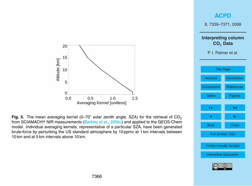
MACHY scenes. We take into account the vertical sensitivity of SCIAMACHY to

changes in CO2 by using the instrument averaging kernel, A. The averaging kernel15

formally describes the sensitivity of retrieved CO2 columns to changes in CO2 through-

out the column, and is a reflection of atmospheric radiative transfer at NIR wavelengths.

Figure 5 shows the mean SCIAMACHY averaging kernel, averaged over solar zenith

angles ranging from 0

to 70, increase in sensitivity throughout the troposphere with

only a small fall-off in the last 1 km (Barkley et al., 2006c). As noted above, not taking20

A into account compromises subsequent interpretation of observed columns. Model

SCIAMACHY CO2 columns, Ω, are given by (Rodgers, 2000)

Ω = Ωa + a(H(x) − xa), (1)

where H(x) is the GEOS-Chem forward model, xa is the a priori CO2 concentration

profile taken from climatology and also used in the SCIAMACHY retrievals (Remedios25

et al., 2006) and Ωa is the associated column. The column averaging kernel a is given

7348





ACPD

8, 7339–7371, 2008

Interpreting column

CO2 Data

P. I. Palmer et al.

Title Page



Tables Figures

Back Close

Full Screen / Esc



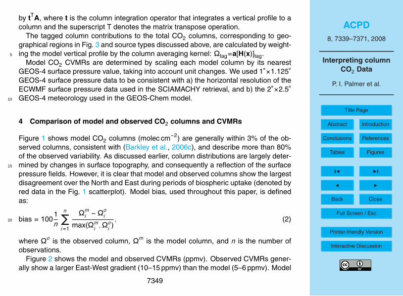
by tTA, where t is the column integration operator that integrates a vertical profile to a

column and the superscript T denotes the matrix transpose operation.

The tagged column contributions to the total CO2 columns, corresponding to geo-

graphical regions in Fig. 3 and source types discussed above, are calculated by weight-

ing the model vertical profile by the column averaging kernel: Ωtag=a[H(x)]tag.5

Model CO2 CVMRs are determined by scaling each model column by its nearest

GEOS-4 surface pressure value, taking into account unit changes. We used 1×1.125

GEOS-4 surface pressure data to be consistent with a) the horizontal resolution of the

ECWMF surface pressure data used in the SCIAMACHY retrieval, and b) the 2×2.5

GEOS-4 meteorology used in the GEOS-Chem model.10

4 Comparison of model and observed CO2 columns and CVMRs

Figure 1 shows model CO2 columns (molec cm−2

) are generally within 3% of the ob-

served columns, consistent with (Barkley et al., 2006c), and describe more than 80%

of the observed variability. As discussed earlier, column distributions are largely deter-

mined by changes in surface topography, and consequently a reflection of the surface15

pressure fields. However, it is clear that model and observed columns show the largest

disagreement over the North and East during periods of biospheric uptake (denoted by

red data in the Fig. 1 scatterplot). Model bias, used throughout this paper, is defined

as:

bias = 1001

n

n∑

i=1

Ωm

i−Ω

o

i

max(Ωm

i,Ω

o

i), (2)20

where Ωo

is the observed column, Ωm

is the model column, and n is the number of

observations.

Figure 2 shows the model and observed CVMRs (ppmv). Observed CVMRs gener-

ally show a larger East-West gradient (10–15 ppmv) than the model (5–6 ppmv). Model

7349





ACPD

8, 7339–7371, 2008

Interpreting column

CO2 Data

P. I. Palmer et al.

Title Page



Tables Figures

Back Close

Full Screen / Esc



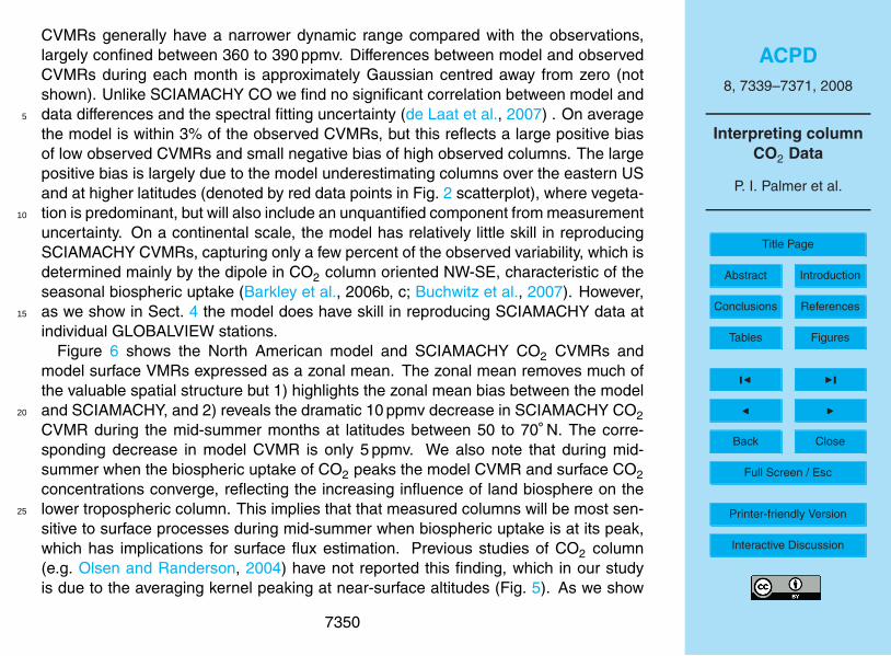
CVMRs generally have a narrower dynamic range compared with the observations,

largely confined between 360 to 390 ppmv. Differences between model and observed

CVMRs during each month is approximately Gaussian centred away from zero (not

shown). Unlike SCIAMACHY CO we find no significant correlation between model and

data differences and the spectral fitting uncertainty (de Laat et al., 2007) . On average5

the model is within 3% of the observed CVMRs, but this reflects a large positive bias

of low observed CVMRs and small negative bias of high observed columns. The large

positive bias is largely due to the model underestimating columns over the eastern US

and at higher latitudes (denoted by red data points in Fig. 2 scatterplot), where vegeta-

tion is predominant, but will also include an unquantified component from measurement10

uncertainty. On a continental scale, the model has relatively little skill in reproducing

SCIAMACHY CVMRs, capturing only a few percent of the observed variability, which is

determined mainly by the dipole in CO2 column oriented NW-SE, characteristic of the

seasonal biospheric uptake (Barkley et al., 2006b, c; Buchwitz et al., 2007). However,

as we show in Sect. 4 the model does have skill in reproducing SCIAMACHY data at15

individual GLOBALVIEW stations.

Figure 6 shows the North American model and SCIAMACHY CO2 CVMRs and

model surface VMRs expressed as a zonal mean. The zonal mean removes much of

the valuable spatial structure but 1) highlights the zonal mean bias between the model

and SCIAMACHY, and 2) reveals the dramatic 10 ppmv decrease in SCIAMACHY CO220

CVMR during the mid-summer months at latitudes between 50 to 70N. The corre-

sponding decrease in model CVMR is only 5 ppmv. We also note that during mid-

summer when the biospheric uptake of CO2 peaks the model CVMR and surface CO2

concentrations converge, reflecting the increasing influence of land biosphere on the

lower tropospheric column. This implies that that measured columns will be most sen-25

sitive to surface processes during mid-summer when biospheric uptake is at its peak,

which has implications for surface flux estimation. Previous studies of CO2 column

(e.g. Olsen and Randerson, 2004) have not reported this finding, which in our study

is due to the averaging kernel peaking at near-surface altitudes (Fig. 5). As we show

7350





ACPD

8, 7339–7371, 2008

Interpreting column

CO2 Data

P. I. Palmer et al.

Title Page



Tables Figures

Back Close

Full Screen / Esc



later, outside of the peak North American growing period other CO2 sources and sinks

play a comparable role in determining the column distribution.

5 What surface fluxes determine model CO2 CVMR variability over North Amer-

ica?

5.1 Continental-scale distributions5

Figure 7 shows the land-based contributions to CO2 CVMRs over North America (Fig. 3

and Table 1). Many source and sink terms show large seasonal cycles in their CVMR

contributions. Background CO2 CVMRs (January 2003 initial conditions in our calcula-

tions, Sect. 3) are typically greater than 350 ppmv (not shown).

CO2 columns over North America are determined largely by local sources and sinks,10

as expected. The North American land biosphere (BS NA) represents the single largest

contribution to total CO2, with a minimum and maximum of −8 ppmv and 3 ppmv, re-

spectively, corresponding to a maximum of 1.1% of the total column. This contribution,

here determined by the CASA model (Sect. 3), is a source of CO2 until late May, after

which it becomes a sink peaking in July. During periods of uptake it is characterized by15

a dipole with uptake over the North and East and a source over the arid southwestern

states Barkley et al. (2006b, c). A similar pattern is evident in model and observed total

columns and CVMRs (Figs. 1 and 2). Fuel sources from North America (FL NA) are

relatively constant in magnitude throughout the year (Table 1), with the largest CVMR

contributions over the East coast (up to 0.5 ppmv). The North American biomass burn-20

ing (BB NA) season starts in Canada in June reaching a peak in August with partial

monthly mean columns of 1 ppmv; this contribution, in particular, is likely to be much

larger on sub-monthly timescales and finer spatial scales.

We also show that CO2 columns over North America are significantly influenced

by Boreal Asia and mainland Asia and that in some months these column contribu-25

tions are comparable in magnitude to North American fluxes. Column contributions

7351





ACPD

8, 7339–7371, 2008

Interpreting column

CO2 Data

P. I. Palmer et al.

Title Page



Tables Figures

Back Close

Full Screen / Esc



from Boreal Asian fuel sources (FL BA) are largest over Alaska and northern Canada,

reflecting the latitude of Boreal Asia and subsequent atmospheric transport. Similar

spatial distributions are shown for biomass burning and the land-biosphere from Bo-

real Asia (BS BA), with the contribution from biomass burning peaking in mid-summer.

The land-biosphere is most positive during April (1.2 ppmv) and is most negative during5

July (−5 ppmv). The seasonal cycle of BS BA is similar to that of the North American

biosphere (BS NA), which may compromise the ability of column observations to in-

dependently estimate fluxes from the North American and Boreal Asian biospheres

despite exhibiting different spatial distribution in column space. The largest mainland

Asian fuel and biomass burning contributions (FL AS, BB AS) to North American CO210

occur in March (not shown) and April over the west Coast, consistent with current un-

derstanding of the temporal continental outflow from that region (Liu et al., 2003). The

biospheric signal from mainland Asia (BS AS) is delayed relative to North America with

a negative peak in August. European column contributions from fuel, biomass burn-

ing, and the land biosphere (FL EU, BB EU, BS EU) are qualititively similar to Boreal15

Asia, reflecting similar high latitude atmospheric transport, but they are an order of

magnitude smaller.

Many of these sources and sinks will be much higher on sub-monthly temporal scales

and on finer spatial scales but our results reiterate previous studies that emphasize the

importance of sub-1% precision column measurements if physically meaningful surface20

flux distributions of CO2 are to be estimated.

5.2 Temporal distributions at individual sites

Figures 8 and 9 show the CO2 flux signatures that determine the variability of CO2

at two measurement sites: the WLEF television tower, 12 km east of Park Falls in

Wisconsin and Wendover in Utah. Earlier, in Fig. 4, we showed that GEOS-Chem had25

some skill in reproducing the seasonal cycle of CO2 at both these sites, but predicted

premature uptake of CO2 at the Parks Falls site. We chose these two sites for this

analysis because they exhibit different seasonal cycles.

7352





ACPD

8, 7339–7371, 2008

Interpreting column

CO2 Data

P. I. Palmer et al.

Title Page



Tables Figures

Back Close

Full Screen / Esc



As in Fig. 4 we sample the model at the location of the two ground-based sites and at

the SCIAMACHY overpass time when data is available. The WLEF site shows a sea-

sonal cycle with a peak-to-peak range of 20 ppmv, which is captured reasonably well

by GEOS-Chem. The corresponding model CO2 columns vary by 3×1020

molec cm−2

,

representing a change of order 4% in the column. SCIAMACHY reproduces the broad-5

scale seasonal cycle observed at the surface (and the tower data at this site (Barkley

et al., 2007)) but because of noise, due to the retrieval and the relatively coarse spatial

colocation (Barkley et al., 2007), it is difficult to assess whether SCIAMACHY repro-

duces the later onset of the uptake observed by surface measurements. We use a

30-point running mean to effectively reduce random noise. The resulting smoothed10

observed columns, even after accounting for the bias, show a larger drawdown of CO2

during midsummer. Model and observed CVMRs show greater discrepancy during

midsummer months. Figure 8d shows the seasonal contributions of different monthly

sources and sinks to model CVMRs >0.5 ppmv at some time during the year. Fuel

combustion from North America, Europe and mainland Asia increase throughout the15

year, as expected, with a mean gradient of 1.5 ppmv/year. The North American bio-

sphere at this site makes a significant contribution to the total CO2 CVMR, with smaller

but significant contributions from Boreal Asia, Europe and mainland Asia. The different

continental biosphere signals peak at different times, due to differences in seasonal cy-

cles and atmospheric transport. Biomass burning from Boreal Asia plays only a small20

role in determining CO2 CVMRs at this site, peaking in the Spring. Based on this cal-

culation it is difficult to attribute differences between model and observed CO2 CMVRs

to bias in the magnitude or timing of different continental biosphere fluxes. However, as

we discuss in the next section these subtle differences may help to spatially disagre-

gate CO2 fluxes using formal inverse models.25

Figure 9 shows model and observed columns and CVMRs at Wendover, Utah. The

seasonal cycle at this site is weaker than at WLEF, with a peak-to-peak range of

10 ppmv. SCIAMACHY (smoothed) columns have a negative bias similar in magni-

tude to observed columns at the WLEF site. Model and observed CVMRS are gen-

7353





ACPD

8, 7339–7371, 2008

Interpreting column

CO2 Data

P. I. Palmer et al.

Title Page



Tables Figures

Back Close

Full Screen / Esc



erally much noisier than at WLEF, reflecting rapid variations in relatively small values

of GEOS-4 surface pressure (790–840 hPa compared with 960–990 hPa at WLEF).

Apparent drawdown of observed and model CO2 columns and CVMRs at this site is

much weaker than at the WLEF site. Figure 9d shows the seasonal contributions of

different monthly sources and sinks to model CVMRs >0.5 ppmv at some time during5

the year. As at WLEF there is a strong fuel signature originating from North America,

Europe, and mainland Asia with a similar gradient through the year. From our analysis

the weak seasonal cycle is determined by biospheric signals from Boreal and mainland

Asia, which is not obvious from interpreting total column data.

6 Implications for surface flux estimation10

The ultimate goal of space-borne CO2 data are to locate and quantify natural sources

and sinks of CO2 so that more detailed studies can assess their durability with changes

in climate. Generally, an inverse model is required for that purpose. While such a study

is outside the scope of this paper, and will be the subject of forthcoming work, we

calculate the monthly mean Jacobian matrix corresponding to our forward model cal-15

culations to illustrate the ability of these column data to infer individual sources and

sinks of CO2. In general the Jacobian matrix, describing the sensitivity of total CO2

columns to changes in surface sources and sinks, attributes differences between for-

ward model (GEOS-Chem) and observed quantities to specific surface sources and

sinks.20

For illustration only, Fig. 10 shows the monthly mean columns of the Jacobian matrix

for North America, based on Fig. 7 and Table 1. These calculations show that the North

America and Boreal Asia land biosphere signals are among the strongest signals that

can potentially be retrieved independently. While the initial goal of inversions of space-

based CO2 data may be to estimate total fluxes on a continental scale, it is clear that25

the superposition of different continental flux signatures (some which represent 1% of

total CVMRs) complicates the interpretation of such data. However, as we discussed

7354





ACPD

8, 7339–7371, 2008

Interpreting column

CO2 Data

P. I. Palmer et al.

Title Page



Tables Figures

Back Close

Full Screen / Esc



earlier and show in Fig. 7 the distributions of many of the dominant flux signatures are

sufficiently separated in space and time to permit independent estimation of individual

fluxes; this needs to be confirmed with inversion calculations. Many of the sources

and sink of CO2 shown here will have much stronger signatures on finer temporal and

spatial scales and that should also be considered.5

The e-folding lifetime of these individual flux contributions is typically 3 to 4 months,

with e-folding lifetimes exceeding 6 months for Asian sources, consistent with Bruhwiler

et al. (2005). All sensitivities converge to a background sensitivity (20) beyond which

individual source and sink signatures are well mixed. In practice, the inversion will use

a Jacobian matrix for a specific surface grid box to avoid aliasing and to capture the10

sharp temporal gradients in CO2 during the onset and decline of the growing season.

7 Conclusions

We have used the GEOS-Chem global 3-D CTM, driven by a priori sources and sinks of

CO2, to interpret variability of SCIAMACHY CO2 columns. We have shown that GEOS-

Chem has some skill in reproducing observed distributions of surface VMR at sites over15

North America. The magnitude and distribution of model CO2 columns, accounting for

the SCIAMACHY averaging kernel, are determined largely by surface pressure and

show good agreement with SCIAMACHY (r=0.9) as expected but with a 3% positive

bias. Model CO2 CVMRs show much less agreement, partly driven by a large positive

bias in drawdown of CO2 during the growing season. We show that model CVMRs20

and surface VMRs converge during peak growing season months, a result amplified by

the use of the SCIAMACHY averaging kernels that describe how instrument sensitivity

increases as a function of depth in the troposphere. This suggest that SCIAMACHY

and upcoming instruments sensing CO2 at NIR wavelengths will be most sensitive to

periods of intense biospheric uptake (Barkley et al., 2007).25

We have used a tagged approach to interpret variability of CVMRs in terms of in-

dividual source and sink terms. In general, we find local sources provide the largest

7355





ACPD

8, 7339–7371, 2008

Interpreting column

CO2 Data

P. I. Palmer et al.

Title Page



Tables Figures

Back Close

Full Screen / Esc



contributions to CVMR variability, with the North American land biosphere representing

more than 1% during peak growing season. Fuel sources are relatively constant, while

biomass burning makes only a significant contribution in mid-burning season. Our cal-

culations show that surface fluxes from Boreal Asia, mainland Asia and Europe also

represent significant contributions to CVMR variability over North America, with, for in-5

stance, the Boreal Asia land biosphere responsible for almost 1% of the total CVMR

in mid-summer. While there are significant overlaps in the CVMR distributions from

local and non-local fluxes, there is also sufficient separation of these contributions in

time and space that with careful analysis should permit independent flux estimation.

Analysis of data from individual sites within the US provided further insight into the su-10

perposition flux signatures. At the WLEF GLOBALVIEW site near Park Falls, Wisconsin

we showed that the seasonal cycle (peak-to-peak surface VMR of 29 ppmv) was driven

by North American biospheric uptake (−4 ppmv peak) but also biospheric uptake sig-

natures from Boreal Asia, Europe and to a lesser extent mainland Asia. In contrast,

the site at Wendover Utah, with a smaller peak-to-peak seasonal cycle of 10 ppmv had15

large contributions from biospheric uptake signatures originating from Boreal Asia and

mainland Asia, both peaking in late summer with CVMRs of −2 ppmv.

CO2 flux estimation relies partly on quantifying the difference between model and ob-

served CO2 quantities. Prescribed error covariance matrices describe only the random

error associated with the model and observations. Uncharacterized systematic error20

could be mis-attributed to surface source and sinks. Estimating systematic bias with

a model is of little value because our current quantitative understanding of the carbon

cycle is incomplete. Dedicated calibration-validation efforts are underway for upcoming

spaceborne missions. A particular focus, owing to spatial nature of the column data, is

the estimation of regional biases (on spatial scales of 100 km), a length scale lying be-25

tween undetectable effects due to noise and large-scale biases detectable with precise

and accurate ground-based FTS. Unfortunately, no such measurements were available

during 2003. Recent studies have shown that SCIAMACHY CO2 columns VMRs dur-

ing 2004 are within 2% of the ground-based FTS column measurements at Park Falls,

7356





ACPD

8, 7339–7371, 2008

Interpreting column

CO2 Data

P. I. Palmer et al.

Title Page



Tables Figures

Back Close

Full Screen / Esc



Wisconsin, capturing only the monthly mean variability (Barkley et al., 2007). This sug-

gests that CO2 CVMR anomalies might be more effective than CO2 CVMRs as the

measurement vector.

Acknowledgements. P. I. Palmer acknowledges NERC grant NE/F000014/1, M. P. Barkley ac-

knowledges NERC grant NE/D001471/1, and P. S. Monks acknowledges NERC CASIX and5

DARC funding.

References

Barkley, M. P., Frieß, U., and Monks, P. S.: Measuring atmospheric CO2 from space using the

Full Spectral Initiation (FSI) WFM-DOAS, Atmos. Chem. Phys., 6, 3517–3534, 2006a,

http://www.atmos-chem-phys.net/6/3517/2006/. 7343, 734410

Barkley, M. P., Monks, P. S., and Engelen, R. J.: Comparison of SCIAMACHY and AIRS CO2

measurements over North America during the summer and autumn of 2003, Geophys. Res.

Lett., 33, L20805, doi:10.1029/2006GL026807, 2006b. 7351

Barkley, M. P., Monks, P. S., Frieß, U., Mittermeier, R. L., Fast, H., Korner, S., and Heimann,

M.: Comparisons between SCIAMACHY atmospheric CO2 retrieved using (FSI) WFM-DOAS15

to ground based FTIR data and the TM3 chemistry transport model, Atmos. Chem. Phys.,

6, 4483–4498, 2006c, http://www.atmos-chem-phys.net/6/4483/2006/. 7342, 7344, 7345,

7348, 7349, 7350, 7366

Barkley, M. P., Monks, P. S., Hewitt, A. J., Machida, T., Desai, A., Vinnichenko, N., Nakazawa,

T., Arshinov, M. Y., Fedoseev, N., and Watai, T.: Asssessing the near-surface sensitivity of20

SCIAMACHY atmospheric CO2 retrieved using (FSI) WFM-DOAS, Atmos. Chem. Phys., 7,

3597–3619, 2007, http://www.atmos-chem-phys.net/7/3597/2007/. 7353, 7355, 7357

Bousquet, P., Ciais, P., Peylin, P., Ramonet, M., and Monfray, P.: Inverse modeling of annual

atmospheric CO2 sources and sinks: 1. method and control inversion, J. Geophys. Res.,

104, 26 161–26 178, 1999. 734125

Bovensmann, H., Burrows, J. P., Buchwitz, M., Frerick, J., Noel, S., Rozanov, V. V., Chance,

K. V., and Goede, A. H. P.: SCIAMACHY - Mission objectives and measurement modes, J.

Atmos. Sci., 56, 127–150, 1999. 7341, 7343

Bruhwiler, L. M. P., Michalak, A. M., Peters, W., Baker, D. F., and Tans, P.: An improved Kalman

Smoother for atmospheric inversions, Atmos. Chem. Phys., 5, 2691–2702, 2005,30

http://www.atmos-chem-phys.net/5/2691/2005/. 7355

7357





http://www.atmos-chem-phys.net/6/3517/2006/




ACPD

8, 7339–7371, 2008

Interpreting column

CO2 Data

P. I. Palmer et al.

Title Page



Tables Figures

Back Close

Full Screen / Esc



Buchwitz, M., Rozanov, V. V., and Burrows, J. P.: A near-infrared optimized DOAS method for

the fast global retrieval of atmospheric CH4, CO, CO2, H2O, and N2O total column amounts

from SCIAMACHY Envisat-1 nadir radiances, J. Geophys. Res., 105, 15 231–15 246, 2000.

7343

Buchwitz, M., de Beek, R., Burrows, J. P., Bovensmann, H., Warneke, T., Notholt, J., Meirink,5

J. F., Goede, A. P. H., Bergamaschi, P., Korner, S., Heimann, M., and Schulz, A.: Atmo-

spheric methane and carbon dioxide from SCIAMACHY satellite data: initial comparison

with chemistry and transport models, Atmos. Chem. Phys., 5, 941–962, 2005,

http://www.atmos-chem-phys.net/5/941/2005/. 7342

Buchwitz, M., Schneising, O., Burrows, J. P., Bovensmann, H., Reuter, M., and Notholt, J.: First10

direct observation of the atmospheric CO2 year-to-year increase from space, Atmos. Chem.

Phys., 7, 4249–4256, 2007, http://www.atmos-chem-phys.net/7/4249/2007/. 7345, 7350

Chen, J. M., Chen, B., and Tans, P.: Deriving daily carbon fluxes from hourly CO2 mixing

ratios measured on the WLEF tall tower: An upscaling methodology, J. Geophys. Res., 112,

G01015, doi:10.1029/2006JG000280, 2007. 734115

Chevallier, F., Breon, F., and Rayner, P. J.: Contribution of the Orbiting Carbon Observatory to

the estimation of CO2 sources and sinks: Theoretical study in a variational data assimilation

framework, J. Geophys. Res., 112, D09307, doi:10.1029/2006JD007375, 2007. 7341

Corbin, K. D., Denning, A. S., Lu, L., Wang, J.-W., and Baker, I. T.: Possible represen-

tation errors in inversions of satellite CO2 retrievals, J. Geophys. Res., 113, D02301,20

doi:10.1029/2007JD008716, 2008. 7342

Crisp, D., Atlas, R. M., Breon, F. M., Brown, L. R., Burrows, J. P., Ciais, P., Connor, B. J.,

Doney, S. C., Fung, I. Y., Jacob, D. J., Miller, C. E., O’Brien, D., Pawson, S., Randerson,

J. T., Rayner, P., Salawitch, R. J., Sander, S. P., Sen, B., Stephens, G. L., Tans, P. P., Toon,

G. C., Wennberg, P. O., Wofsy, S. C., Yung, Y. L., Kuang, Z., Chudasama, B., Sprague, G.,25

Weiss, B., Pollock, R., Kenyon, D., and Schroll, S.: The Orbiting Carbon Observatory (OCO)

mission, Adv. Space Res., 34, 700–709, 2004. 7341

de Laat, A. T. J., Gloudemans, A. M. S., Aben, I., Krol, M., Meirink, J. F., van der Werf, G. R.,

and Schrijver, H.: Scanning Imaging Absorption Spectrometer for Atmospheric Chartogra-

phy carbon monoxide total columns: statistical evaluation and comparison with chemistry30

transport model results, J. Geophys. Res., 112, D12310, doi:10.1029/2006JD008256, 2007.

7350

GLOBALVIEW-CO2: GLOBALVIEW-CO2: Cooperative Atmospheric Data Project – Carbon

7358







ACPD

8, 7339–7371, 2008

Interpreting column

CO2 Data

P. I. Palmer et al.

Title Page



Tables Figures

Back Close

Full Screen / Esc



Dioxide, CD-ROM, NOAA GMD, Boulder, Colorado (Also available via anonymous FTP to

ftp.cmdl.noaa.gov, path: ccg/co2/GLOBALVIEW), 2006. 7343, 7347, 7365

Gurney, K. R., Law, R. M., Denning, A. S., Rayner, P. J., Baker, D., Bousquet, P., Bruhwiler,

L., Chen, Y.-H., Ciais, P., Fan, S., Fung, I. Y., Gloor, M., Heimann, M., Higuchi, K., John,

J., Maki, T., Maksyutov, S., Masarie, K., Peylin, P., Prather, M., Pak, B. C., Randerson,5

J., Sarmiento, J., Taguchi, S., Takahashi, T., and Yuen, C.-W.: Towards robust regional esti-

mates of CO2 sources and sinks using atmospheric transport models, Nature, 415, 626–630,

doi:10.1038/415626a, 2002. 7341

Hamazaki, T., Kuze, A., and Kondo, K.: Sensor system for Greenhouse gas Observing SATellite

(GOSAT), Proc. SPIE, 5543, doi:10.1117/12.560589, 2004. 734110

IPCC: Climate Change 2007 – The Physical Basis, Contribution of Working Group I to the

Fourth Assessment Report of the IPCC, Cambridge University Press, iSBN 978 0521

880099-1, 2007. 7341

Krijger, J. M., Aben, I., and Schrijver, H.: Distinction between clouds and ice/snow covered

surfaces in the identification of cloud-free observations using SCIAMACHY PMDs, Atmos.15

Chem. Phys., 5, 2279–2738, 2005, http://www.atmos-chem-phys.net/5/2279/2005/. 7344

Liu, H. Y., Jacob, D. J., Bey, I., Yantosca, R. M., Duncan, B. N., and Sachse, G. W.: Transport

pathways for Asian combustion outflow over the Pacific: Interannual and seasonal variations,

J. Geophys. Res., 108(D20), 8786, doi:10.1029/2002JD003102, 2003. 7352

Marland, G., Boden, T. A., and Andres, R. J.: Global, Regional, and National CO2 Emissions, in:20

Trends: A Compendium of Data on Global Change, Tech. rep., Carbon Dioxide Information

Analysis Center, Oak Ridge National Laboratory, US Department of Energy, Oak Ridge,

Tenn., USA, 2007. 7346

Miller, C. E., Crisp, D., DeCola, P. L., Olsen, S. C., Randerson, J. T., Michalak, A. M., Alkhaled,

A., Rayner, P., Jacob, D. J., Suntharalingam, P., Jones, D. B. A., Denning, A. S., Nicholls,25

M. E., Doney, S. C., Pawson, S., Boesch, H., Connor, B. J., Fung, I. Y., O’Brien, D., Salawitch,

R. J., Sander, S. P., Sen, B., Tans, P., Toon, G. C., Wennberg, P. O., Wofsy, S. C., Yung, Y. L.,

and Law, R. M.: Precision requirements for space-based XCO2data, J. Geophys. Res., 112,

D10314, doi:10.1029/2006JD007659, 2007. 7341, 7342

Olsen, S. C. and Randerson, J. T.: Differences between surface and column atmo-30

spheric CO2 and implications for carbon cycle research, J. Geophys. Res., 109, D02301,

doi:10.1029/2003JD003968, 2004. 7342, 7345, 7350

Palmer, P. I., Suntharalingam, P., Jones, D. B. A., Jacob, D. J., Streets, D. G., Fu, Q., Vay, S. A.,

7359





ftp.cmdl.noaa.gov


ACPD

8, 7339–7371, 2008

Interpreting column

CO2 Data

P. I. Palmer et al.

Title Page



Tables Figures

Back Close

Full Screen / Esc



and Sachse, G. W.: Using CO2:CO correlations to improve inverse analyses of carbon fluxes,

J. Geophys. Res., 111, D12318, doi:10.1029/2005JD006697, 2006. 7341, 7346, 7347

Randerson, J. T., Thompson, M. V., Conway, T. J., Fung, I. Y., and Field, C. B.: The contribution

of terrestrial sources and sinks to trends in the seasonal cycle of atmospheric carbon dioxide,

Global Biogeochem. Cycles, 11, 535–560, 1997. 73465

Rayner, P. J. and O’Brien, D. M.: The utility of remotely sensed CO2 concentration data in

surface source inversions, Geophys. Res. Lett., 28, 175–178, 2001. 7342

Remedios, J. H., Parker, R. J., Panchal, M., Leigh, R. J., and Corlett, G.: Signatures of atmo-

spheric and surface climate variables through analyses of infrared spectra (SATSCAN-IR),

in: Proceedings of the first EPS/METOP RAO workshop, ESRIN, 2006. 734810

Rodgers, C. D.: Inverse methods for atmospheric sounding, World Scientific, 2000. 7348

Stephens, B. B., Gurney, K. R., Tans, P. P., Sweeney, C., Peters, W., Bruhwiler, L., Ciais, P.,

Ramonet, M., Bousquet, P., Nakazawa, T., Aoki, S., Machida, T., Inoue, G., Vinnichenko, N.,

Lloyd, J., Jordan, A., Heimann, M., Shibistova, O., Langenfelds, R. L., Steele, L. P., Francey,

R. J., and Denning, A. S.: Weak Northern and Strong Tropical Land Carbon Uptake from15

Vertical Profiles of Atmospheric CO2, Science, 316, 1732–1735, 2007. 7341

Suntharalingam, P., Jacob, D. J., Palmer, P. I., Logan, J. A., Yantosca, R. M., Xiao, Y., and

Evans, M. J.: Improved quantification of Chinese carbon fluxes using CO2/CO correlations

in Asian outflow, J. Geophys. Res., 109, D18S18, doi:10.1029/2003JD004362, 2004. 7346,

734720

Suntharalingam, P., Randerson, J. T., Krakauer, N., Jacob, D. J., and Logan, J. A.: The in-

fluence of reduced carbon emissions and oxidation on the distribution of atmospheric CO2:

implications for inversion analysis, 19, GB4003, doi:10.1029/2005GB002466, 2005. 7346

Takahashi, T., Wanninkhof, R. T., Feely, R. A., Weiss, R. F., Chapman, D. W., Bates, N. R.,

Olafsson, J., Sabine, C. L., and Sutherland, C. S.: Net sea-air CO2 flux over the global25

oceans, in: Proceedings of the 2nd international symposium CO2 in the oceans: CGER

1037, pp. 9–15, National Institute for Environmental Studies, Tsukuba, Japan, 1999. 7346

van der Werf, G. R., Randerson, J. T., Giglio, L., Collatz, G. J., Kasibhatla, P. S., and Arellano Jr.,

A. F.: Interannual variability in global biomass burning emissions from 1997–2004, Atmos.

Chem. Phys., 6, 3423–3441, 2006, http://www.atmos-chem-phys.net/6/3423/2006/. 734630

Yevich, R. and Logan, J. A.: An assessment of biofuel use and burning of agricultural waste in

the developing world, Global Biogeochem. Cycles, 17, 1095, doi:10.1029/2002GB001952,

2003. 7346

7360






ACPD

8, 7339–7371, 2008

Interpreting column

CO2 Data

P. I. Palmer et al.

Title Page



Tables Figures

Back Close

Full Screen / Esc



Table 1. Monthly mean regional CO2 fluxes (Tg CO2/month) for the forward model analysis

(Sect. 3 and Fig. 3). BB denotes biomass burning; FL denotes the sum of fossil fuel and biofuel

combustion; and BS denotes the land biosphere. ROW includes only land-based sources and

sinks; the ocean biosphere is an annual global net sink of −8050 Tg CO2/yr. Boreal Asia

(BA) is defined by 72.5E–172.5

W, 45

N–88

N; mainland Asia (AS) is defined by 72.5

E–

152.5E, 8

N–45

N; Europe (EU) is defined by 17.5

E–72.5

W, 36

N–88

N; North America

(NA) defined by 172.5E–17.5

E, 24

N–88

N; and the rest of the world (ROW) is the remaining

region.

Jan Feb Mar Apr May Jun Jul Aug Sep Oct Nov Dec

BB

BA 0 0 21 124 486 233 196 80 26 13 1 0

AS 29 37 93 89 15 5 4 5 5 4 3 9

EU 0 0.5 6 21 17 6 14 39 34 30 0.3 0.2

NA 2 1 3 6 7 44 36 95 22 14 9 1

ROW 895 463 360 262 891 774 801 853 669 427 360 668

FL

BA 53 47 53 51 53 51 53 53 51 53 51 53

AS 808 730 808 730 808 730 808 808 730 808 730 808

EU 570 514 570 551 570 551 570 570 551 570 551 570

NA 563 508 563 545 563 545 563 563 545 563 545 563

ROW 475 429 475 460 475 460 475 475 460 475 460 475

BS

BA 374 401 563 657 64 −1469 −1818 −952 459 770 542 408

AS 288 484 763 797 243 −363 −916 −1141 −456 −12 127 180

EU 534 455 333 −98 −1068 −1491 −1284 −307 651 892 772 630

NA 703 709 729 496 −248 −1692 −1981 −1167 33 834 838 747

ROW −101 −322 −350 119 −139 −1385 −1431 −578 952 1363 1099 771

7361





ACPD

8, 7339–7371, 2008

Interpreting column

CO2 Data

P. I. Palmer et al.

Title Page



Tables Figures

Back Close

Full Screen / Esc



SCIAMACHY CO2

APR

GEOS-Chem CO

2

6 7 8 9SCIAMACHY CO

2[1021 molec/cm2]

6

7

8

9

GE

OS

-Che

m C

O2

[1021

mol

ec/c

m2 ]

r = 0.94n = 455

Bias = 1.98%

6.00 7.00 8.00 9.00[1021 molec cm-2]

MAY

6 7 8 9SCIAMACHY CO

2[1021 molec/cm2]

6

7

8

9

GE

OS

-Che

m C

O2

[1021

mol

ec/c

m2 ]

r = 0.93n = 487

Bias = 2.51%

6.00 7.00 8.00 9.00[1021 molec cm-2]

JUN

6 7 8 9SCIAMACHY CO

2[1021 molec/cm2]

6

7

8

9

GE

OS

-Che

m C

O2

[1021

mol

ec/c

m2 ]

r = 0.95n = 430

Bias = 2.99%

6.00 7.00 8.00 9.00[1021 molec cm-2]

JUL

6 7 8 9SCIAMACHY CO

2[1021 molec/cm2]

6

7

8

9

GE

OS

-Che

m C

O2

[1021

mol

ec/c

m2 ]

r = 0.95n = 498

Bias = 2.91%

6.00 7.00 8.00 9.00[1021 molec cm-2]

AUG

6 7 8 9SCIAMACHY CO

2[1021 molec/cm2]

6

7

8

9

GE

OS

-Che

m C

O2

[1021

mol

ec/c

m2 ]

r = 0.95n = 422

Bias = 2.36%

6.00 7.00 8.00 9.00[1021 molec cm-2]

SEP

6 7 8 9SCIAMACHY CO

2[1021 molec/cm2]

6

7

8

9

GE

OS

-Che

m C

O2

[1021

mol

ec/c

m2 ]

r = 0.96n = 491

Bias = 2.13%

6.00 7.00 8.00 9.00[1021 molec cm-2]

Fig. 1. Monthly mean SCIAMACHY (left) and GEOS-Chem (middle) CO2 columns

(1021

molec cm−2

) over North America during April to September 2003 averaged over the

GEOS-Chem 2×2.5

grid. The model is sampled at the time and location of the observed

scenes, and using the SCIAMACHY averaging kernel as outlined in the main text. The RHS

panels show scatterplots of the monthly mean data, with the number of data points n, correla-

tion coefficient r , and the model bias inset. Red data denote columns over the region defined

by latitudes >50N and longitudes >100

W (as shown in top LHS panel). We exclude 1) cloudy

scenes, identified by instrument polarization devices, 2) scenes with solar zenith angles >75,

3) scenes with a retrieval errors of ≥5%, and 4) scenes that correspond to CVMRs outside of

the range 340–400 ppmv. 7362





ACPD

8, 7339–7371, 2008

Interpreting column

CO2 Data

P. I. Palmer et al.

Title Page



Tables Figures

Back Close

Full Screen / Esc



SCIAMACHY CO2

APR

GEOS-Chem CO

2

340 360 380 400SCIAMACHY CO

2[ppmv]

340

360

380

400

GE

OS

-Che

m C

O2

[ppm

v]

r = -0.13n = 455Bias = 1.76%

340 360 380 400[ppmv]

MAY


2[ppmv]

340

360

380

400

GE

OS

-Che

m C

O2

[ppm

v]

r = -0.11n = 487Bias = 2.39%

340 360 380 400[ppmv]

JUN


2[ppmv]

340

360

380

400

GE

OS

-Che

m C

O2

[ppm

v]

r = 0.07n = 430Bias = 2.88%

340 360 380 400[ppmv]

JUL


2[ppmv]

340

360

380

400

GE

OS

-Che

m C

O2

[ppm

v]

r = 0.24n = 498Bias = 2.78%

340 360 380 400[ppmv]

AUG


2[ppmv]

340

360

380

400

GE

OS

-Che

m C

O2

[ppm

v]

r = 0.24n = 422Bias = 2.26%

340 360 380 400[ppmv]

SEP


2[ppmv]

340

360

380

400

GE

OS

-Che

m C

O2

[ppm

v]r = 0.07n = 491

Bias = 1.99%

340 360 380 400[ppmv]

Fig. 2. Monthly mean SCIAMACHY and GEOS-Chem CO2 CVMRs (ppmv) over North America

during April to September 2003 averaged over the GEOS-Chem 2×2.5

grid. The model and

data descriptions are as Fig. 1. The nearest ECMWF (1.125×1.125

) and GEOS-4 (1

×1.125

)

surface pressure data are used to convert from observed and model columns to CVMRs, re-

spectively.

7363





ACPD

8, 7339–7371, 2008

Interpreting column

CO2 Data

P. I. Palmer et al.

Title Page



Tables Figures

Back Close

Full Screen / Esc



-135 -90 -45 0 45 90 135

-135 -90 -45 0 45 90 135

-60

-30

030

60

-60-30

030

60

NA

EU BA

AS

ROW

Fig. 3. Source regions for the tagged CO2 simulation. The regions are denoted boreal Asia

(BA), mainland Asia (AS), Europe (EU), North America (NA) and the rest of the world (ROW).

See Table 1 for latitude and longitude region definitions and associated flux estimates.

7364





ACPD

8, 7339–7371, 2008

Interpreting column

CO2 Data

P. I. Palmer et al.

Title Page



Tables Figures

Back Close

Full Screen / Esc



2002.5 2003.0 2003.5 2004.0 2004.5Julian day

350

367

383

400

CO

2 VM

R [p

pmv] Alert, Nunavut, Canada

GLOBALVIEW GEOS-Chem

2002.5 2003.0 2003.5 2004.0 2004.5Julian day

350

367

383

400

CO

2 VM

R [p

pmv] Barrow, Alaska, United States


2002.5 2003.0 2003.5 2004.0 2004.5Julian day

350

367

383

400C

O2 V

MR

[ppm

v] Estevan Point, British Columbia, Canada


2002.5 2003.0 2003.5 2004.0 2004.5Julian day

350

367

383

400

CO

2 VM

R [p

pmv] Fraserdale, Ontario, Canada


2002.5 2003.0 2003.5 2004.0 2004.5Julian day

350

367

383

400

CO

2 VM

R [p

pmv] Harvard Forest, Massachusetts, United States


2002.5 2003.0 2003.5 2004.0 2004.5Julian day

350

367

383

400

CO

2 VM

R [p

pmv] Park Falls, Wisconsin, United States


2002.5 2003.0 2003.5 2004.0 2004.5Julian day

350

367

383

400

CO

2 VM

R [p

pmv] Niwot Ridge, Colorado, United States


2002.5 2003.0 2003.5 2004.0 2004.5Julian day

350

367

383

400

CO

2 VM

R [p

pmv] Wendover, Utah, United States


Fig. 4. Comparison of observed (GLOBALVIEW-CO2, 2006) and model surface CO2 concen-

trations (ppmv) over North America during 2003. Model concentrations, averaged on a 2×2.5

,

have been sampled at the overpass time of SCIAMACHY when data are available.

7365





ACPD

8, 7339–7371, 2008

Interpreting column

CO2 Data

P. I. Palmer et al.

Title Page



Tables Figures

Back Close

Full Screen / Esc



0.0 0.5 1.0 1.5Averaging Kernel [unitless]

0

5

10

15

20

Alti

tude

[km

]

Fig. 5. The mean averaging kernel (0–70

solar zenith angle, SZA) for the retrieval of CO2

from SCIAMACHY NIR measurements (Barkley et al., 2006c) and applied to the GEOS-Chem

model. Individual averaging kernels, representative of a particular SZA, have been generated

brute-force by perturbing the US standard atmosphere by 10 ppmv at 1 km intervals between

10 km and at 5 km intervals above 10 km.

7366





ACPD

8, 7339–7371, 2008

Interpreting column

CO2 Data

P. I. Palmer et al.

Title Page



Tables Figures

Back Close

Full Screen / Esc



30 40 50 60 70 80Latitude [Deg]

350

360

370

380

390

CO

2 CV

MR

and

VM

R [p

pmv]

Model (CVMR)

Model (sfc VMR)

Data (CVMR) APR

30 40 50 60 70 80Latitude [Deg]

350

360

370

380

390

CO

2 CV

MR

and

VM

R [p

pmv]

Model (CVMR)

Model (sfc VMR)

Data (CVMR) MAY

30 40 50 60 70 80Latitude [Deg]

350

360

370

380

390

CO

2 CV

MR

and

VM

R [p

pmv]

Model (CVMR)

Model (sfc VMR)

Data (CVMR) JUN

30 40 50 60 70 80Latitude [Deg]

350

360

370

380

390

CO

2 CV

MR

and

VM

R [p

pmv]

Model (CVMR)

Model (sfc VMR)

Data (CVMR) JUL

30 40 50 60 70 80Latitude [Deg]

350

360

370

380

390C

O2 C

VM

R a

nd V

MR

[ppm

v]Model (CVMR)

Model (sfc VMR)

Data (CVMR) AUG

30 40 50 60 70 80Latitude [Deg]

350

360

370

380

390

CO

2 CV

MR

and

VM

R [p

pmv]

Model (CVMR)

Model (sfc VMR)

Data (CVMR) SEP

Fig. 6. Monthly mean latitude gradients of SCIAMACHY and GEOS-Chem CO2 CVMRs (ppmv)

and GEOS-Chem surface VMR (ppmv) over North America during April–September 2003

binned every 5

latitude. Model concentrations, averaged on a 2×2.5

, have been sampled

at the overpass time of SCIAMACHY when data are available. Filled triangles denote mean

values and open circles denote median values. Vertical lines denote the 1-standard deviation

about the mean values.

7367





ACPD

8, 7339–7371, 2008

Interpreting column

CO2 Data

P. I. Palmer et al.

Title Page



Tables Figures

Back Close

Full Screen / Esc



FL NA

APR

FL EU

APR

FL BA

APR

FL AS

APR

BB NA

APR

BB EU

APR

BB BA

APR

BB AS

APR

BS NA

APR

BS EU

APR

BS BA

APR

BS AS

APR

CVMR [ppmv]

MAY

MAY

MAY

MAY

MAY

MAY

MAY

MAY

MAY

MAY

MAY

MAY

CVMR [ppmv]

JUN

JUN

JUN

JUN

JUN

JUN

JUN

JUN

JUN

JUN

JUN

JUN

CVMR [ppmv]

JUL

JUL

JUL

JUL

JUL

JUL

JUL

JUL

JUL

JUL

JUL

JUL

CVMR [ppmv]

AUG

AUG

AUG

AUG

AUG

AUG

AUG

AUG

AUG

AUG

AUG

AUG

CVMR [ppmv]

0.0 2.0

SEP

0.0 0.2

SEP

0.0 0.1

SEP

0.0 0.4

SEP

0.0 0.5

SEP

0.0 0.1

SEP

0.0 0.5

SEP

0.0 0.1

SEP

-4.0 3.0

SEP

-0.2 0.2

SEP

-2.0 1.0

SEP

-1.0 1.0

SEP

CVMR [ppmv]

Fig. 7. Monthly mean GEOS-Chem CO2 CVMR contributions (ppmv) from continental sources

and sinks during April to September 2003, averaged over the GEOS-Chem 2×2.5

grid. See

Fig. 3 for source region definitions and Table 1 for regional CO2 flux estimates.

7368





ACPD

8, 7339–7371, 2008

Interpreting column

CO2 Data

P. I. Palmer et al.

Title Page



Tables Figures

Back Close

Full Screen / Esc



Fig. 8. CO2 surface concentrations, columns, and CVMRs at the WLEF television tower,

Wisconsin USA (45.94N, 90.27

W, 442 m above sea level) during 2003. (A) GLOB-

ALVIEW and GEOS-Chem model, averaged on a 2×2.5

grid, surface CO2 concentrations

(ppmv), (B) SCIAMACHY (raw and 30-point running average) and GEOS-Chem CO2 columns

[1021

molec cm−2

], (C) SCIAMACHY (raw and 30-point running average) and GEOS-Chem

CVMR (ppmv), and (D) GEOS-Chem CVMR contributions greater than 0.5 ppmv.

7369





ACPD

8, 7339–7371, 2008

Interpreting column

CO2 Data

P. I. Palmer et al.

Title Page



Tables Figures

Back Close

Full Screen / Esc


Interactive DiscussionFig. 9. CO2 surface concentrations, columns, and CVMRs at Wendover, Utah USA (39.9

N,

−113.72W, 1320 m above sea level) during 2003. Individual panels follow Fig. 8.

7370





ACPD

8, 7339–7371, 2008

Interpreting column

CO2 Data

P. I. Palmer et al.

Title Page



Tables Figures

Back Close

Full Screen / Esc



FL NA

0 2 4 6 8 10 12Month in 2003

020406080

100

dCV

MR

/dE

mon

th i

JAN FEB MAR APR MAY JUNJUL AUG SEP OCT NOV DEC

BS NA

0 2 4 6 8 10 12Month in 2003

020406080

100

dCV

MR

/dE

mon

th i BB NA

0 2 4 6 8 10 12Month in 2003

020406080

100

dCV

MR

/dE

mon

th i

FL BA

0 2 4 6 8 10 12Month in 2003

020406080

100

dCV

MR

/dE

mon

th i BS BA

0 2 4 6 8 10 12Month in 2003

020406080

100

dCV

MR

/dE

mon

th i BB BA

0 2 4 6 8 10 12Month in 2003

020406080

100

dCV

MR

/dE

mon

th i

FL EU

0 2 4 6 8 10 12Month in 2003

020406080

100

dCV

MR

/dE

mon

th i BS EU

0 2 4 6 8 10 12Month in 2003

020406080

100dC

VM

R/d

Em

onth

i BB EU

0 2 4 6 8 10 12Month in 2003

020406080

100

dCV

MR

/dE

mon

th i

FL AS

0 2 4 6 8 10 12Month in 2003

020406080

100

dCV

MR

/dE

mon

th i BS AS

0 2 4 6 8 10 12Month in 2003

020406080

100

dCV

MR

/dE

mon

th i BB AS

0 2 4 6 8 10 12Month in 2003

020406080

100

dCV

MR

/dE

mon

th i

Fig. 10. Monthly mean columns of the Jacobian matrix (ppmv/Tg CO2), scaled by 105

for pre-

sentation, calculated using a priori flux estimates (Table 1) and the corresponding GEOS-Chem

CVMR contributions, averaged on a 2×2.5

grid over North America during 2003 (Fig. 7).

Colours denote specific months . Each point represents the monthly mean sensitivity of North

American CO2 columns to specific continental sources and sinks. Lines connecting the points

have no physical significance.

7371





Interpreting the variability of CO2 columns over North ...

Documents

Transcript of Interpreting the variability of CO2 columns over North ...