Interpreting Pressure and Flow Rate Data from Permanent ...
263
INTERPRETING PRESSURE AND FLOW RATE DATA FROM PERMANENT DOWNHOLE GAUGES USING DATA MINING APPROACHES A DISSERTATION SUBMITTED TO THE DEPARTMENT OF ENERGY RESOURCES ENGINEERING AND THE COMMITTEE ON GRADUATE STUDIES OF STANFORD UNIVERSITY IN PARTIAL FULFILLMENT OF THE REQUIREMENTS FOR THE DEGREE OF DOCTOR OF PHILOSOPHY Yang Liu March 2013
Transcript of Interpreting Pressure and Flow Rate Data from Permanent ...

INTERPRETING PRESSURE AND FLOW RATE DATA
FROM PERMANENT DOWNHOLE GAUGES
USING DATA MINING APPROACHES
A DISSERTATION
SUBMITTED TO THE DEPARTMENT OF ENERGY
RESOURCES ENGINEERING
AND THE COMMITTEE ON GRADUATE STUDIES
OF STANFORD UNIVERSITY
IN PARTIAL FULFILLMENT OF THE REQUIREMENTS
FOR THE DEGREE OF
DOCTOR OF PHILOSOPHY
Yang Liu
March 2013

http://creativecommons.org/licenses/by-nc/3.0/us/
This dissertation is online at: http://purl.stanford.edu/xp635wx9603
© 2013 by Yang Liu. All Rights Reserved.
Re-distributed by Stanford University under license with the author.
This work is licensed under a Creative Commons Attribution-Noncommercial 3.0 United States License.
ii

I certify that I have read this dissertation and that, in my opinion, it is fully adequatein scope and quality as a dissertation for the degree of Doctor of Philosophy.
Roland Horne, Primary Adviser
I certify that I have read this dissertation and that, in my opinion, it is fully adequatein scope and quality as a dissertation for the degree of Doctor of Philosophy.
Margot Gerritsen
I certify that I have read this dissertation and that, in my opinion, it is fully adequatein scope and quality as a dissertation for the degree of Doctor of Philosophy.
Tapan Mukerji
Approved for the Stanford University Committee on Graduate Studies.
Patricia J. Gumport, Vice Provost Graduate Education
This signature page was generated electronically upon submission of this dissertation in electronic format. An original signed hard copy of the signature page is on file inUniversity Archives.
iii

Abstract
The Permanent Downhole Gauge (PDG) is a promising resource for real time down-
hole measurement. However, a bottleneck in utilizing the PDG data is that the
commonly applied well test methods are limited (practically) to short sections of
shut-in data only and thus fail to utilize the long term PDG data. Recent technology
developments have provided the ability for PDGs to measure both flow rate and pres-
sure, so the limitation of using only shut-in periods could be avoided, theoretically. In
practice however it is still difficult to make use of the combined flow rate and pressure
data over a PDG record of long duration, due to the noise in both of the signals as
well as uncertainty with respect to the appropriate reservoir model over such a long
period.
The successful application of data mining in computer science shows great poten-
tial in revealing the relationship between variables from voluminous data sets. This
inspired us to investigate the application of data mining methodologies as a way to
reveal the relationship between flow rate and pressure histories from PDG data, and
hence extract the reservoir model.
In this study, nonparametric kernel-based data mining approaches were studied.
The data mining process was conducted in two stages, namely learning and prediction.
In the learning process, the reservoir model was obtained implicitly in a suitable
functional form in the high-dimensional kernel Hilbert space (defined by the kernel
function) when the learning algorithm converged after being trained to the pressure
and flow rate data. In the prediction process, a pressure prediction was made by the
data mining algorithm according to an arbitrary flow rate history (usually a constant
flow rate history for simplicity). This flow rate history and the corresponding pressure
iv

prediction revealed the reservoir model underlying the variable PDG data. In a second
mode, recalculating the pressure history based on the measured flow rate history
removed noise from the pressure signal effectively. Recalculating the pressure based
on a denoised flow rate history removed noise from both signals.
In the work, a series of data mining methods using different kernel functions
and input vectors were investigated. Methods A, B, and C utilized simple kernel
functions. Method A and Method B did not require the knowledge of breakpoints
in advance. The difference between the two was that Method A used a low-order
kernel function with a high-order input vector, while Method B used a high-order
kernel function with a low-order input vector. Method C required the knowledge of
the breakpoints. Nine synthetic test cases with different well/reservoir models were
used to test these methods. The results showed that all three methods have good
pressure reproduction of the training flow rate history and pressure prediction of the
constant flow rate history. However, each of them has limitations in different aspects.
The limitation of the simple kernel methods led us to a reconsideration of ker-
nelization and superposition. In the simple kernel methods, the kernelization was
deployed over the superposition which was reflected as the summation in the input
vector. However, the architecture of superposition over kernelization would be more
suitable to capture the essence of the transient, and this approach was implemented
by using a convolution kernel in Method D. The convolution kernel was invented and
applied in the domain of natural language machine learning. In the original linguis-
tic study, the convolution kernel decomposed words into parts, and evaluated the
parts using a simple kernel function. This inspired us to apply the convolution kernel
method to PDG data by decomposing the pressure transient into a series of pressure
responses to the previous flow rate change events. The superposition was then re-
flected as the summation of simple kernels (hence superposition over kernelization).
16 synthetic and real field test cases were tested using this approach. The method
recovered the reservoir model successfully in all cases. By comparison, Method D
outperformed all simple kernel methods for its stability and accuracy in all test cases
without knowing the breakpoints in advance.
v

This study also discussed the performance of Method D working under compli-
cated data situations, including the existence of significant outliers and aberrant seg-
ments, incomplete production history, unknown initial pressure, different sampling
frequencies, and different time spans of the data set. The results suggested that: 1)
Method D tolerated a moderate level of outliers and aberrant segments without any
preprocessing; 2) Method D might reveal the reservoir/well model with effective rate
correction and/or optimization on initial pressure value when the production history
was incomplete and/or when the initial pressure was unknown; and 3) an appropri-
ate sampling frequency and time span of the data set were required to ensure the
sufficiency of the basis functions in the Hilbert kernel space.
In order to improve the performance of the convolution kernel method in dealing
with large data sets, two block algorithms, namely Methods E and F, were also
investigated. The two methods rescaled the original kernel matrix into a series of
block matrices, and used only some of the blocks to complete the training process. A
series of synthetic cases and real cases illustrated their efficiency and accuracy. The
comparison of the performance between Methods D, E, and F was also conducted.
vi

Acknowledgements
At the time when my Ph.D study finally approaches to an end, there is a long list of
names that I would like to show my thanks to. In my five-year journey of graduate
study, some of them pointed the direction for me many a time, encouraging me to
persist in my research despite failures; some of them lent me their hands once I
met problems no matter whether in the daily life or academic study; and some of
them accompanied me day after day, sharing my happiness and sadness. It is their
guidance, help and care that supported me to reach today’s status.
The first person that I would like to appreciate is my advisor, Professor Roland
Horne. He was the professor that recruited me in Beijing when I applied to the
department for admission nearly six years ago. He was also my advisor who guided
both my master’s and Ph.D study. Many a time when I hesitated trying a new
idea that might very possibly fail the tests, he always encouraged me to go ahead.
His warm words, “proving that a method does not work for a case is still a part of
research”, comforted me a lot when the research reached a plateau. His remarkable
insight and precise intuition helped me keeping on the right track of study. His
creative thoughts always provided me with more ideas. I feel lucky and honored
being his student in my graduate study. I still remember the first day when I saw
him in his office in 2007, he said “Yang, we have a long we to go.” Today, the way
reaches a milestone but does not end. I will cherish these days with Professor Horne,
and maintain this close personal relationship carefully in the future.
I would also like to express my gratitude to the rest of my thesis committee mem-
bers: Professor Margot Gerritsen, Professor Tapan Mukerji, Professor Lou Durlofsky,
and Professor Norman Sleep. Each of them helped me in my academic growth and
vii

gave constructive comments to my thesis and research. Professor Margot Gerritsen’s
linear algebra course gave me a solid foundation in the mathematic theory and com-
putation. Professor Tapan Mukerji has a wide range of knowledge, so that his courses
and talks were always good resources of references. As one of organizers of Smart
Field Annual Conference, Professor Lou Durlofsky provided a series constructive com-
ments and suggestions to my research work which was presented in the meeting. I
owe thanks to Professor Norman Sleep as well. Although I was not familiar to him,
he was still willing to be my committee chairman, and read through my thesis and
discuss the details with me. His attitude towards the scientific study earned my great
respect.
To the Smart Field Consortium and SUPRI-D Research Group, I express my
sincere thankfulness as well. The two research groups provided me not only the
important financial support throughout my whole graduate study, but also friendly
interactive academic platforms. I am grateful to Professor Khalid Aziz as he always
kept an eye on my research process suggesting me to widen the usage of my study as
a generic petroleum data processing method. The weekly SUPRI-D group meeting
was a joyful event in a busy life. I enjoyed the free discussion and knowledge sharing
between all SUPRI-D members. Especially, my acknowledgements go to Priscila
Ribeiro, Sanghui Ahn, Zhe Wang, and Maytham Ibrahim Al Ismail. They never
stinted their encouragement whenever I obtained a little progress.
Five years of campus life provided me chances to meet a lot of friends that cared
for me and cherished our friendship. I thank Siyao Xu, my roommate and best
friend, for his kindness, help, and generousness. I also thank Thanapong Boontaeng,
my officemate, for his patience many a time when I presented him the progress of
my research. I owe thanks to the Chinese community as well. Their friendship and
support made it easy in my daily life.
To my parents and my wife, I express my utmost love and acknowlegement. Nei-
ther of my parents has attended university due to the limitation in the special period
of China’s history. However, they always encouraged me to complete the Ph.D study
despite any difficulties. I appreciate them for giving me a life to experience such
exciting education and meet so many friends. I owe everything to my wife, Zhizhen
viii

Liu. She accompanied me in the long journey of my graduate study, sharing all my
happiness and sadness. Her persistent love supported every step of my progress. I
leave my final sincere gratitude to my devoted wife.
ix

This page intentionally left blank.
x

Contents
Abstract iv
Acknowledgements vii
1 Introduction 1
1.1 Problem Statement . . . . . . . . . . . . . . . . . . . . . . . . . . . . 4
1.2 Methodology . . . . . . . . . . . . . . . . . . . . . . . . . . . . . . . 8
1.3 Dissertation Outline . . . . . . . . . . . . . . . . . . . . . . . . . . . 11
2 Literature Review 14
2.1 Reservoir Monitoring and Management . . . . . . . . . . . . . . . . . 15
2.2 Pressure Transient Analysis . . . . . . . . . . . . . . . . . . . . . . . 17
2.2.1 Data Processing and Denoising . . . . . . . . . . . . . . . . . 18
2.2.2 Breakpoint Detection . . . . . . . . . . . . . . . . . . . . . . . 22
2.2.3 Flow Rate Reconstruction . . . . . . . . . . . . . . . . . . . . 25
2.2.4 Change of Reservoir Properties . . . . . . . . . . . . . . . . . 27
2.3 Deconvolution . . . . . . . . . . . . . . . . . . . . . . . . . . . . . . . 30
2.4 Temperature Transient Analysis . . . . . . . . . . . . . . . . . . . . . 34
2.5 Data Mining . . . . . . . . . . . . . . . . . . . . . . . . . . . . . . . . 37
3 Data Mining Concept and Simple Kernel 40
3.1 Components of Learning Algorithm . . . . . . . . . . . . . . . . . . . 41
3.1.1 Model . . . . . . . . . . . . . . . . . . . . . . . . . . . . . . . 42
3.1.2 Cost Function . . . . . . . . . . . . . . . . . . . . . . . . . . . 43
xi

3.1.3 Optimization Search Method . . . . . . . . . . . . . . . . . . . 45
3.2 Kernelization . . . . . . . . . . . . . . . . . . . . . . . . . . . . . . . 48
3.3 Kernelized Data Mining without Breakpoint Detection . . . . . . . . 53
3.4 Kernelized Data Mining with Breakpoint Detection . . . . . . . . . . 57
3.5 Application on Synthetic Cases . . . . . . . . . . . . . . . . . . . . . 59
3.5.1 Radial Flow . . . . . . . . . . . . . . . . . . . . . . . . . . . . 61
3.5.2 Radial Flow + Wellbore . . . . . . . . . . . . . . . . . . . . . 61
3.5.3 Radial Flow + Skin . . . . . . . . . . . . . . . . . . . . . . . . 61
3.5.4 Radial Flow + Wellbore + Skin . . . . . . . . . . . . . . . . . 64
3.5.5 Radial Flow + Closed Boundary . . . . . . . . . . . . . . . . . 64
3.5.6 Radial Flow + Constant Pressure Boundary . . . . . . . . . . 65
3.5.7 Radial Flow + Wellbore + Skin + Closed Boundary . . . . . . 65
3.5.8 Radial Flow + Wellbore + Skin + Constant Boundary . . . . 67
3.5.9 Radial Flow + Dual Porosity . . . . . . . . . . . . . . . . . . 67
3.6 Summary and Limitation . . . . . . . . . . . . . . . . . . . . . . . . . 68
4 Convolution Kernel 72
4.1 The Origination of Convolution Kernel . . . . . . . . . . . . . . . . . 72
4.2 Convolution Kernel Applied to PDG Data . . . . . . . . . . . . . . . 75
4.3 Conjugate Gradient . . . . . . . . . . . . . . . . . . . . . . . . . . . . 77
4.4 Input Vector Selection . . . . . . . . . . . . . . . . . . . . . . . . . . 83
4.5 Application . . . . . . . . . . . . . . . . . . . . . . . . . . . . . . . . 87
4.5.1 Radial Flow . . . . . . . . . . . . . . . . . . . . . . . . . . . . 91
4.5.2 Radial Flow + Wellbore . . . . . . . . . . . . . . . . . . . . . 93
4.5.3 Radial Flow + Skin . . . . . . . . . . . . . . . . . . . . . . . . 95
4.5.4 Radial Flow + Wellbore + Skin . . . . . . . . . . . . . . . . . 95
4.5.5 Radial Flow + Closed Boundary . . . . . . . . . . . . . . . . . 96
4.5.6 Radial Flow + Constant Pressure Boundary . . . . . . . . . . 98
4.5.7 Radial Flow + Wellbore + Skin + Closed Boundary . . . . . . 98
4.5.8 Radial Flow + Wellbore + Skin + Constant Boundary . . . . 99
4.5.9 Radial Flow + Dual Porosity . . . . . . . . . . . . . . . . . . 102
xii

4.5.10 Complicated Synthetic Case A . . . . . . . . . . . . . . . . . . 103
4.5.11 Complicated Synthetic Case B . . . . . . . . . . . . . . . . . . 105
4.5.12 Semireal Case A . . . . . . . . . . . . . . . . . . . . . . . . . 107
4.5.13 Semireal Case B . . . . . . . . . . . . . . . . . . . . . . . . . . 109
4.5.14 Real Case A . . . . . . . . . . . . . . . . . . . . . . . . . . . . 109
4.5.15 Real Case B . . . . . . . . . . . . . . . . . . . . . . . . . . . . 111
4.5.16 Real Case C . . . . . . . . . . . . . . . . . . . . . . . . . . . . 115
4.6 Summary . . . . . . . . . . . . . . . . . . . . . . . . . . . . . . . . . 115
5 Performance Analysis 119
5.1 Outliers . . . . . . . . . . . . . . . . . . . . . . . . . . . . . . . . . . 120
5.2 Aberrant Segments . . . . . . . . . . . . . . . . . . . . . . . . . . . . 127
5.3 Partial Production History . . . . . . . . . . . . . . . . . . . . . . . . 136
5.4 Unknown Initial Pressure . . . . . . . . . . . . . . . . . . . . . . . . . 143
5.5 Sampling Frequency . . . . . . . . . . . . . . . . . . . . . . . . . . . 148
5.6 Evolution of Learning . . . . . . . . . . . . . . . . . . . . . . . . . . . 154
5.7 Summary . . . . . . . . . . . . . . . . . . . . . . . . . . . . . . . . . 158
6 Rescalability 162
6.1 Block Algorithm . . . . . . . . . . . . . . . . . . . . . . . . . . . . . 163
6.2 Advanced Block Algorithm . . . . . . . . . . . . . . . . . . . . . . . . 170
6.3 Real Data Application . . . . . . . . . . . . . . . . . . . . . . . . . . 173
6.4 Summary . . . . . . . . . . . . . . . . . . . . . . . . . . . . . . . . . 178
7 Conclusion and Future Work 180
A Data 186
B Proof of Kernel Closure Rules 213
B.1 Summation Closure . . . . . . . . . . . . . . . . . . . . . . . . . . . . 213
B.2 Tensor Product Closure . . . . . . . . . . . . . . . . . . . . . . . . . 214
B.3 Positive Scaling Closure . . . . . . . . . . . . . . . . . . . . . . . . . 215
xiii

C Breakpoint Detection Using Data Mining Approaches 217
C.1 K-means and Bilateral . . . . . . . . . . . . . . . . . . . . . . . . . . 217
C.2 Minimum Message Length . . . . . . . . . . . . . . . . . . . . . . . . 220
D Implementation 225
D.1 Classes . . . . . . . . . . . . . . . . . . . . . . . . . . . . . . . . . . . 225
D.2 Work Flow . . . . . . . . . . . . . . . . . . . . . . . . . . . . . . . . . 229
Nomenclature 234
Bibliography 237
xiv

List of Tables
3.1 Kernel Function and the Corresponding Φ (x) (Ng, 2009) . . . . . . . 51
3.2 Reservoir behavior and input features . . . . . . . . . . . . . . . . . . 55
3.3 Input vectors and kernel functions for Method A and Method B . . . 56
3.4 Input vector and kernel function for Method C . . . . . . . . . . . . . 58
3.5 Test cases for simple kernel method . . . . . . . . . . . . . . . . . . . 60
4.1 Input vector for convolution kernel . . . . . . . . . . . . . . . . . . . 84
4.2 Test cases for convolution kernel input vector selection . . . . . . . . 85
4.3 Input vector and kernel function for Method D . . . . . . . . . . . . . 88
4.4 Test cases for convolution kernel method . . . . . . . . . . . . . . . . 89
4.5 Result plots for all tests on convolution kernel method . . . . . . . . 92
5.1 Test cases for outliers performance analysis . . . . . . . . . . . . . . . 122
5.2 Test cases for aberrant segment performance analysis . . . . . . . . . 129
5.3 Test case for partial production history performance analysis . . . . . 138
5.4 Test case for partial production history performance analysis . . . . . 140
5.5 Test case for unknown initial pressure performance analysis . . . . . . 145
5.6 Test case for unknown initial pressure analysis . . . . . . . . . . . . . 147
5.7 Test cases for sampling frequency performance analysis . . . . . . . . 150
5.8 Test cases for evolution learning performance analysis . . . . . . . . . 155
6.1 Comparison between Method D and Method E . . . . . . . . . . . . . 166
6.2 Test cases for rescalability test using Method E . . . . . . . . . . . . 167
6.3 Comparison between Method E and Method F . . . . . . . . . . . . . 171
xv

6.4 Test cases for rescalability test using Method F . . . . . . . . . . . . 172
6.5 Test cases for rescalability test on large PDG data set . . . . . . . . . 175
6.6 Execution time of Case 36 with different block sizes . . . . . . . . . . 178
A.1 Data for Case 1 . . . . . . . . . . . . . . . . . . . . . . . . . . . . . . 186
A.2 Data for Case 2 . . . . . . . . . . . . . . . . . . . . . . . . . . . . . . 186
A.3 Data for Case 3 . . . . . . . . . . . . . . . . . . . . . . . . . . . . . . 187
A.4 Data for Case 4 . . . . . . . . . . . . . . . . . . . . . . . . . . . . . . 187
A.5 Data for Case 5 . . . . . . . . . . . . . . . . . . . . . . . . . . . . . . 187
A.6 Data for Case 6 . . . . . . . . . . . . . . . . . . . . . . . . . . . . . . 188
A.7 Data for Case 7 . . . . . . . . . . . . . . . . . . . . . . . . . . . . . . 188
A.8 Data for Case 8 . . . . . . . . . . . . . . . . . . . . . . . . . . . . . . 189
A.9 Data for Case 9 . . . . . . . . . . . . . . . . . . . . . . . . . . . . . . 189
A.10 Data for Case 10 . . . . . . . . . . . . . . . . . . . . . . . . . . . . . 190
A.11 Data for Case 11 . . . . . . . . . . . . . . . . . . . . . . . . . . . . . 190
A.12 Data for Case 12 . . . . . . . . . . . . . . . . . . . . . . . . . . . . . 191
A.13 Data for Case 13 . . . . . . . . . . . . . . . . . . . . . . . . . . . . . 191
A.14 Data for Case 14 . . . . . . . . . . . . . . . . . . . . . . . . . . . . . 192
A.15 Data for Case 15 . . . . . . . . . . . . . . . . . . . . . . . . . . . . . 195
A.16 Data for Cases 16-18 . . . . . . . . . . . . . . . . . . . . . . . . . . . 199
A.17 Data for Cases 19-22 . . . . . . . . . . . . . . . . . . . . . . . . . . . 199
A.18 Data for Cases 23-24 . . . . . . . . . . . . . . . . . . . . . . . . . . . 200
A.19 Data for Cases 25-26 . . . . . . . . . . . . . . . . . . . . . . . . . . . 200
A.20 Data for Cases 27-30 . . . . . . . . . . . . . . . . . . . . . . . . . . . 201
A.21 Data for Cases 31-34 . . . . . . . . . . . . . . . . . . . . . . . . . . . 201
A.22 Data for Cases 35 . . . . . . . . . . . . . . . . . . . . . . . . . . . . . 202
A.23 Data for Cases 36-37 . . . . . . . . . . . . . . . . . . . . . . . . . . . 202
xvi

List of Figures
1.1 The structure of PDG . . . . . . . . . . . . . . . . . . . . . . . . . . 2
1.2 The appearance of PDG . . . . . . . . . . . . . . . . . . . . . . . . . 3
1.3 Variable flow rate and noisy data from PDG . . . . . . . . . . . . . . 6
1.4 Detect the real reservoir response . . . . . . . . . . . . . . . . . . . . 7
1.5 Discover the real reservoir model . . . . . . . . . . . . . . . . . . . . 8
1.6 Work Flow . . . . . . . . . . . . . . . . . . . . . . . . . . . . . . . . . 10
2.1 Pressure response of a slant well . . . . . . . . . . . . . . . . . . . . . 15
2.2 History matching using PDG data . . . . . . . . . . . . . . . . . . . . 16
2.3 A general downhole data acquisition system . . . . . . . . . . . . . . 19
2.4 Three categories of noise from PDG . . . . . . . . . . . . . . . . . . . 20
2.5 Fitting pressure data with two approaches . . . . . . . . . . . . . . . 22
2.6 Breakpoint detection with both pressure and the flow rate data . . . 24
2.7 The effect of inaccuracy in breakpoint detection . . . . . . . . . . . . 25
2.8 Flow rate reconstruction using PDG pressure data . . . . . . . . . . . 26
2.9 Flow rate reconstruction using wavelet transformation . . . . . . . . . 28
2.10 History matching with variable reservoir properties . . . . . . . . . . 29
2.11 Variable reservoir properties as functions of time . . . . . . . . . . . . 29
2.12 Variable reservoir properties using the moving window method . . . . 30
2.13 Piecewise constant reservoir properties . . . . . . . . . . . . . . . . . 31
2.14 Deconvolution applied on the simulated data . . . . . . . . . . . . . . 32
2.15 Recover the initial pressure by deconvolution . . . . . . . . . . . . . . 33
2.16 Deconvolution with convex optimization on real field data . . . . . . 34
2.17 Temperature and pressure data from a PDG . . . . . . . . . . . . . . 35
xvii

2.18 Temperature and pressure transient analysis . . . . . . . . . . . . . . 36
2.19 Pressure prediction on synthetic data . . . . . . . . . . . . . . . . . . 38
2.20 Pressure prediction on real data . . . . . . . . . . . . . . . . . . . . . 38
3.1 Superposition . . . . . . . . . . . . . . . . . . . . . . . . . . . . . . . 54
3.2 Demonstration of the construction of feature-based input variable. . . 58
3.3 Simple kernel learning results for Case 1 . . . . . . . . . . . . . . . . 62
3.4 Simple kernel learning results for Case 2 . . . . . . . . . . . . . . . . 63
3.5 Simple kernel learning results for Case 3 . . . . . . . . . . . . . . . . 63
3.6 Simple kernel learning results for Case 4 . . . . . . . . . . . . . . . . 64
3.7 Simple kernel learning results for Case 5 . . . . . . . . . . . . . . . . 65
3.8 Simple kernel learning results for Case 6 . . . . . . . . . . . . . . . . 66
3.9 Simple kernel learning results for Case 7 . . . . . . . . . . . . . . . . 66
3.10 Simple kernel learning results for Case 8 . . . . . . . . . . . . . . . . 67
3.11 Simple kernel learning results for Case 9 . . . . . . . . . . . . . . . . 68
3.12 Method B failed to predict on a more variable flow rate history . . . . 70
4.1 Decompose an input sample point into parts . . . . . . . . . . . . . . 75
4.2 Comparison between SGD and CG . . . . . . . . . . . . . . . . . . . 78
4.3 Comparison between different convolution input vectors . . . . . . . . 86
4.4 Convolution kernel learning results for Case 1 . . . . . . . . . . . . . 94
4.5 Convolution kernel learning results for Case 2 . . . . . . . . . . . . . 95
4.6 Convolution kernel learning results for Case 3 . . . . . . . . . . . . . 96
4.7 Convolution kernel learning results for Case 4 . . . . . . . . . . . . . 97
4.8 Convolution kernel learning results for Case 5 . . . . . . . . . . . . . 98
4.9 Convolution kernel learning results for Case 6 . . . . . . . . . . . . . 99
4.10 Convolution kernel learning results for Case 7 . . . . . . . . . . . . . 100
4.11 Convolution kernel learning results for Case 8 . . . . . . . . . . . . . 101
4.12 Convolution kernel learning results for Case 9 . . . . . . . . . . . . . 102
4.13 Convolution kernel learning results for Case 10 . . . . . . . . . . . . . 104
4.14 Convolution kernel learning results for Case 11 . . . . . . . . . . . . . 106
4.15 Convolution kernel learning results for Case 12 . . . . . . . . . . . . . 108
xviii

4.16 Convolution kernel learning results for Case 13 . . . . . . . . . . . . . 110
4.17 Convolution kernel learning results for Case 14 . . . . . . . . . . . . . 112
4.18 Convolution kernel learning results for Case 15 . . . . . . . . . . . . . 113
4.19 Comparison between the prediction of two real cases . . . . . . . . . 114
4.20 Convolution kernel learning results for Case 37 . . . . . . . . . . . . . 116
5.1 Outlier performance test on Case 16 . . . . . . . . . . . . . . . . . . . 123
5.2 Outlier performance test on Case 17 . . . . . . . . . . . . . . . . . . . 125
5.3 Outlier performance test on Case 18 . . . . . . . . . . . . . . . . . . . 126
5.4 Aberrant segment performance test on Case 19 . . . . . . . . . . . . . 131
5.5 Aberrant segment performance test on Case 20 . . . . . . . . . . . . . 132
5.6 Aberrant segment performance test on Case 21 . . . . . . . . . . . . . 134
5.7 Aberrant segment performance test on Case 22 . . . . . . . . . . . . . 135
5.8 The original complete data set for Cases 23 and 24 . . . . . . . . . . 137
5.9 Partial production history test on Case 23 . . . . . . . . . . . . . . . 139
5.10 Partial production history test on Case 24 A . . . . . . . . . . . . . . 141
5.11 Partial production history test on Case 24 B . . . . . . . . . . . . . . 142
5.12 The true data and training data for Cases 25 and 26 . . . . . . . . . 144
5.13 Unknown initial pressure performance test on Case 25 . . . . . . . . . 145
5.14 Unknown initial pressure performance test on Case 26 . . . . . . . . . 148
5.15 The original complete data set for Cases 27-30 . . . . . . . . . . . . . 149
5.16 Pressure reproduction in the frequency tests on Cases 27 - 30 . . . . . 151
5.17 Pressure prediction in the frequency tests on Cases 27 - 30 . . . . . . 153
5.18 The original complete data set for Cases 31-34 . . . . . . . . . . . . . 155
5.19 Pressure reproduction in the evolution tests on Cases 31 - 34 . . . . . 157
5.20 Pressure prediction in the evolution tests on Cases 31-34 . . . . . . . 159
6.1 The block matrices used in the block algorithm . . . . . . . . . . . . 165
6.2 Rescalability test results on Case 35 using Method E . . . . . . . . . 169
6.3 The block matrices used in the advanced block algorithm . . . . . . . 170
6.4 Rescalability test results on Case 35 using Method E . . . . . . . . . 174
6.5 The real field data for rescalability tests . . . . . . . . . . . . . . . . 175
xix

6.6 The real field data and the resampled data for Cases 36 . . . . . . . . 176
6.7 Rescalability test results on Cases 36 . . . . . . . . . . . . . . . . . . 177
C.1 K-means and Bilateral methods on breakpoint detection . . . . . . . 219
C.2 MML method on breakpoint detection (no outliers) . . . . . . . . . . 222
C.3 MML method on breakpoint detection (outliers) . . . . . . . . . . . . 223
C.4 MML method usign flow Rate and time data only . . . . . . . . . . . 224
D.1 The class diagram of the PDG project . . . . . . . . . . . . . . . . . 226
D.2 The work flow of tests . . . . . . . . . . . . . . . . . . . . . . . . . . 230
xx

Chapter 1
Introduction
Downhole data acquisition from a producing well is very important for petroleum
development mainly for two reasons. On one hand, the real time measurements will
enable the petroleum engineers to access the immediate well status, so that a quick
response may be taken if any abnormal reservoir behaviours were observed. On the
other, the accumulated downhole data may be used to better calibrate the reser-
voir model in a history matching process, in which a reservoir model is proposed to
match the obtained measurements and thereafter to predict the future performance
of the reservoir. Conventionally, only the surface measurements such as surface rates
and cumulative production volume are utilized in a history matching process. The
downhole production data including pressure, flow rate and temperature as the func-
tions of time, may improve the accuracy of the reservoir model by capturing more
details of real time reservoir behaviours. Based on the prediction of the improved
model, petroleum engineers may make complex decisions to optimize the long term
production.
However, although the importance of real time downhole measurement is recog-
nized in the petroleum industry, long-term continuous downhole measurement was
not feasible due to the technical limitation until the invention and the deployment of
the Permanent Downhole Gauge(PDG).
Permanent Downhole Gauges were designed initially for well monitoring. The
installation of PDGs may date back to as far as 1963 (Nestlerode, 1963). However,
1

CHAPTER 1. INTRODUCTION 2
they were not widely deployed until the late 1980s when a new generation of reliable
PDGs was developed (Horne, 2007; Eck et al., 2000).
Figure 1.1: The structure of a commercial PDG (Eck et al., 2000).
Fig. 1.1 demonstrates the structure of a commercial PDG, while Fig. 1.2 shows
the appearance of a PDG used in offshore reservoirs. At the early stages, the PDG
measured only the temperature and the pressure, and was not able to obtain the flow
rate information. Therefore, at that time, only the temperature and pressure existed
in the PDG data set.
However, with the further development of PDGs, this problem was overcome. In
one commercial downhole device, two pressure gauges in gauge mandrels measure

CHAPTER 1. INTRODUCTION 3
Figure 1.2: The appearance of a commercial PDG used in offshore reser-voirs (Konopczynski and McKay, 2009).
the pressure drop across an integrated venturi, which is directly proportional to the
square of the fluid velocity. A third pressure gauge may be used to measure fluid
density. By using these two measurements, the flow rate may be calculated. Other
forms of flow rate measurement are used in permanent downhole gauge configurations
by other service companies. These settings enable the permanent downhole gauges
to provide the pressure, temperature, fluid density and fluid rate simultaneously at
each time point.
Since the 1960s when the first PDG was installed, a half century has passed. The
modern PDGs have more functionalities and better accuracy and stability. More
than 1000 wells worldwide had been equipped with PDGs in 2001 (Khong, 2001),
and the number is possibly close to 20,000 in 2012. The development of the PDG
could be viewed by the milestones of the PDG application in a major oilfield service
company (Eck et al., 2000).
1973 First permanent downhole gauge installation in West Africa, based on wireline
logging cable and equipment.
1975 First pressure and temperature transmitter on a single wireline cable.
1978 First subsea installations in North Sea and West Africa.

CHAPTER 1. INTRODUCTION 4
1983 First subsea installation with acoustic data transmission to surface.
1986 Fully welded metal tubing encased permanent downhole cable.
1986 Introduction of quartz crystal permanent pressure gauge in subsea well.
1990 Fully supported copper conductor in permanent downhole cable.
1993 New generation of quartz and sapphire crystal permanent gauges.
1994 Installation for mass flow rate measurement.
With the ability of long-term continuous record of pressure, flow rate, during
production, the PDG becomes a new and significant source of downhole reservoir
data. However, in many cases, the data from PDGs are still used mainly to monitor
the production status of the well, but not for reservoir analysis. The reason that the
PDG data are not used frequently for reservoir analysis is due to difficulties in dealing
with the uncontrolled flow rate variations in typical PDG data, using conventional
well test interpretation methods. Nevertheless, for the past ten years, petroleum
engineers have persisted in working on how to utilize the huge volume of PDG data
to better characterize the well and the reservoir for reservoir management.
1.1 Problem Statement
From the reservoir engineering point of view, the pressure transient measured by a
PDG is a function of the flow rate changes (the flow rate changes may be calculated
by the flow rates measured by the PDG as well). This is very much like the data
collected in a conventional well test, such as a buildup or a drawdown test (Horne,
2007). However, considering the nature of a conventional well test, an intended control
for an imposed flow rate change, and the nature of PDG measurement, unrestrained
fluctuations in a producing well, there are a few difficulties to apply conventional well
test analysis method to the PDG data.
Firstly, a conventional well test is designed to impose a flow rate change that is
as simple as possible so that the pressure response will be easy to interpret. Fig. 1.3

CHAPTER 1. INTRODUCTION 5
shows a typical pressure and flow rate acquisition from a real PDG. The flow rate data
are variable, and only two small sections of data highlighted in boxes are suitable for a
conventional buildup interpretation. Compared to the huge volume of measurements,
the conventional buildup interpretation methods are only applicable to a very limited
portion of the data.
Secondly, the PDG data are very noisy. Unlike traditional well testing tools that
are used in controlled environments, PDGs measure the pressure and flow rate in the
well during production. Therefore, the uncontrolled nature of the flow introduces
several kinds of noise and artifacts into the data. Fig. 1.3(b) shows a zoom-in view
of Fig. 1.3(a). The flow rate and pressure data are both very noisy. The problem
of the noise is not the absolute value biased from the true data, but the frequent
vibration. This leads to two issues. For the pressure transient, it makes it hard for
us to recognize what is the real reservoir response, and what is due to noise. For the
flow rate, there becomes no easy way to detect the break points (where the flow rate
really changes).
Thirdly, the flow rate history information is not usually needed in the conventional
well test interpretation. In the conventional well test, such as a buildup test or a
drawdown test, the flow rate is intended to be maintained at zero or a constant value.
Nowadays, the PDG has the capability to provide the flow rate information as well,
so there is a strong demand for a method that could cointerpret the pressure as well
as the flow rate simultaneously.
Fourthly, the PDGs measure the pressure and flow rate at a high frequency over
a long duration. A single year of measurement can amount to gigabytes of data. The
volumes of the data are far beyond the capability of manual processing, and thus,
require algorithmic approaches.
In addition to these problems, which are mainly technical difficulties, there is
also a restriction on conventional methods, namely physical model dependency. In
conventional well testing methods, reservoir models, which are used to deduce a re-
lationship between the flow rate and pressure, usually start from predefined physical
equations. This requires the engineer to predefine a physical model before making

CHAPTER 1. INTRODUCTION 6
260 280 300 320 340 360 3808600
8700
8800
8900
9000
Time (hours)
Pre
ssur
e (p
si)
260 280 300 320 340 360 3800
0.5
1
1.5
2
2.5
3x 10
4
Time (hours)
Flo
w R
ate
(ST
B/d
)
(a)
319.4 319.6 319.8 320 320.2 320.4 320.6 320.8 321 321.2 321.48700.5
8701
8701.5
8702
8702.5
8703
8703.5
8704
Time (hours)
Pre
ssur
e (p
si)
319.4 319.6 319.8 320 320.2 320.4 320.6 320.8 321 321.2 321.41.932
1.934
1.936
1.938
1.94
1.942x 10
4
Time (hours)
Flo
w R
ate
(ST
B/d
)
(b)
Figure 1.3: (a) Variable flow rate data. Only two small pieces of data are good for abuildup test. (b) The pressure and flow rate data are both very noisy.

CHAPTER 1. INTRODUCTION 7
any interpretation. This requirement increases the risk of making an incorrect pre-
sumption of physical model, especially bearing in mind that the model must describe
months or years of data, not just a few hours as in a conventional well test. This
study made a major departure from conventional approaches by seeking a physical-
model-independent method to achieve a nonparametric regression, matching a model
without knowing in advance what it is. With plentiful PDG data, the method is ex-
pected to discover the reservoir model in the process, rather than depend on knowing
the model in advance. This is the fundamental premise of this study.
Therefore, the target for this research has been to determine what method is able
to utilize data sets that are: (1) variable in flow rate (2) noisy, and (3) large in
number of measurements, to achieve cointerpretation of the pressure and flow rate
data from permanent downhole gauges with a nonparametric regression. Specifically,
two targets were achieved in this study.
For the first target, we would like to detect the real reservoir response from the
noisy data set. Suppose we have a noisy data set (on the left of Fig. 1.4), our
method will learn and obtain the reservoir properties from the noisy data set. Then,
our method is expected to return a cleaned pressure when the clipped flow rate are
provided (on the right of Fig. 1.4),
Data
0 20 40 60 80 100 120 140 160 180 2004000
4200
4400
4600
4800
5000
5200
Time (hours)
Pre
ssur
e (p
si)
0 20 40 60 80 100 120 140 160 180 200
0
20
40
60
Time (hours)
Flo
w R
ate
(ST
B/d
) =⇒
Cleaned Data
0 20 40 60 80 100 120 140 160 180 2004200
4400
4600
4800
5000
Time (hours)
Pre
ssur
e (p
si)
0 20 40 60 80 100 120 140 160 180 200
0
20
40
60
Time (hours)
Flo
w R
ate
(ST
B/d
)
Figure 1.4: Target 1: Detect the real reservoir response from the noisy data.
As the second target, we would like the method to discover the reservoir model
without knowing it in advance. This is an extension of the first target. Suppose we

CHAPTER 1. INTRODUCTION 8
have a noisy data set from PDGs, our method will learn and obtain the reservoir
model behind the noisy PDG data. After that, the method will give pressure predic-
tion according to an arbitrary given flow rate. In particular, when a constant flow
rate history is provided (as shown in the right part of Fig. 1.5), the predicted pressure
transient corresponding to the given constant flow rate will work like a deconvolu-
tion process, revealing the reservoir model behind the noisy data set.
Data
260 280 300 320 340 360 3808600
8700
8800
8900
9000
Time (hours)
Pre
ssur
e (p
si)
260 280 300 320 340 360 3800
0.5
1
1.5
2
x 104
Time (hours)
Flo
w R
ate
(ST
B/d
) =⇒
Reservoir Model
0 20 40 60 80 100 1207500
8000
8500
9000
9500
10000
Time (hours)
Pre
ssur
e (p
si)
0 20 40 60 80 100 1206
6.5
7
7.5
8x 10
4
Time (hours)
Flo
w R
ate
(ST
B/d
)
Figure 1.5: Target 2: Discover the reservoir model without knowing it in advance.
1.2 Methodology
In order to achieve the research targets, this study investigated the application of data
mining, which is a nonparametric regression method that does not require knowledge
of the reservoir model in advance.
Data mining is the process of extracting patterns from data. Data mining plays
a key role in many areas of science, finance and industry. Here are some examples of
data mining problems:
• Predict the price of a stock 6 months from now, on the basis of company per-
formance measures and economic data (Hastie et al., 2009).
• Identify the numbers in a handwritten ZIP code, from a digitized image (Hastie et al.,
2009).

CHAPTER 1. INTRODUCTION 9
• Search association rules from the supermarket transaction data (Tan et al.,
2005).
• Classify spam or junk emails from incoming emails (Hastie et al., 2009).
• Recognize the face pattern from a data base of photographs to confirm the
identity (Hastie et al., 2009).
Before computers were invented and widely used, manual data mining processes
had been used for centuries. Early methods of identifying patterns in data include
Bayes theorem (1700s) and least square regression analysis (1800s). The development
of computer science technology has stimulated the study of data mining techniques.
In addition to Bayes theorem and least square regression analysis, many efficient and
powerful methods have been invented, including neural networks, genetic algorithm,
decision trees, support vector machine, minimum message length, etc. Most of these
modern data mining methods are computationally intensive, and hence, are computer-
aided. With the help of these methods, many aspects of our daily life are greatly
changed. A typical example is the handwritten ZIP code identification. The neural
network invented in 1950s realized the ZIP code automated recognition. A lot of post
office laborers were released from the tedious work of reading ZIP codes on envelopes.
With the further development of the data mining techniques, the Support Vector
Machine (SVM) method realized identification of handwritten letters with efficient
performance in the 1980s. Nowadays, with the aid of these data mining methods, post
offices are able to process hundreds of thousands of mails faster and more accurately
with fewer manual workers.
Based on data mining’s ability of model detection from large volumes of data,
it seems worthwhile to use data mining in the processing of PDG data. Assuming
the PDG data reflect the properties of the reservoir, proper data mining algorithms
may be able to extract the reservoir model from the PDG data despite them being
variable and noisy. This study focused on applying data mining algorithms in the
cointerpretation of pressure and flow rate signals from permanent downhole gauges.
Fig. 1.6 shows the flow chart of this data mining approach. The whole algorithm
starts from the PDG data including pressure series and flow rate series. Then we

CHAPTER 1. INTRODUCTION 10
Figure 1.6: Work flow chart of cointerpretting pressure and flow rate data from PDGusing data mining approaches.

CHAPTER 1. INTRODUCTION 11
will create a training data set from the raw PDG data to train the machine learning
algorithm. This training process is an iterative process. As long as the machine
learning algorithm converges, the reservoir properties are expected to be obtained
and stored within the algorithm, Then, we may provide an arbitrary flow rate history
(a constant flow rate as an example in Fig. 1.6) as an input, and the well-trained
machine learning algorithm may then give a pressure prediction according to this
given flow rate history. The reservoir properties can be obtained if, as expected, the
pressure prediction can be treated as the real pressure response given the specific new
flow rate history. Also at this time, the original PDG data set, which is noisy, huge in
volume, and variable in flow rate, will be translated into a low-noise constant flow rate
data set. Engineers may apply the conventional well test interpretation methods on
this predicted pressure to estimate more information about the reservoir. Engineers
may even provide a future flow rate projection to ask the algorithm to give pressure
prediction, which could be used for production optimization. In this research, the
kernelization was implemented in the machine learning algorithm, and the training
data set was created according to the selection of different kernel functions.
One of the key reasons for the success of the Support Vector Machine (SVM)
approach is that SVM uses the process of kernelization, which enables the data mining
process to work in a high-dimensional Hilbert space (a space defined by the inner
product of vectors). The main advantage of kernelization is that the data mining is
performed in a very high-dimensional space while the computation is done in a lower-
dimensional space. This work took advantage of this characteristic of kernelization
and applied it in the data mining processing of PDG data.
1.3 Dissertation Outline
This dissertation proceeds as follows.
Chapter 2 provides a literature review on the PDG data interpretation. This
literature review introduces the methodology of previous works in utilizing the PDG
data for well analysis. The advantages and restrictions of the previous methods are
described.

CHAPTER 1. INTRODUCTION 12
Chapter 3 first presents an overview of data mining concepts and introduces the
key components of data mining algorithms. Then it explains the concept and algo-
rithm of kernelization, following which a simple kernel, linear kernel, is discussed.
The simple kernel methods were applied to a series of synthetic cases and the out-
standing issues are discussed in this chapter.
The restrictions of the simple kernel methods discussed in Chapter 3 leads to
an exploration of using a complex kernel, namely the convolution kernel that is
described in Chapter 4. In Chapter 4, the origin of the convolution kernel is first
introduced, followed by the detailed algorithm when using it in the PDG context.
A series of synthetic data, semireal data, and real field data were used to test the
convolution kernel methods. The results are discussed in this chapter as well.
Following Chapter 4, Chapter 5 discusses the performance analysis of the convo-
lution kernel. A series of sensitivity tests was carried out to demonstrate the method
performance in some special real field practice conditions, including the situation with
the existence of outliers and aberrant segments, the situation when the flow rate his-
tory is missing, and the situation with unknown initial pressure. In this chapter, the
effect of training data timespan and training data sampling frequency on the method
performance is also discussed. Finally, a test of evolution learning is also shown to
demonstrate the change of data mining results with time change in a production well.
In Chapter 6, an important issue, the scalability of the data mining method on
huge data sets is investigated. In this chapter, three block learning algorithms are
discussed. The results of applying these methods to a large scale data set are also
present in the final part of this chapter.
Chapter 7 summarizes the whole work, and provides some insights of the possible
future work in the PDG data analysis using data mining approaches.
In addition to the seven chapters, there are four appendices. Appendix A lists all
the data for 37 test cases discussed in the dissertation.
Appendix B proves the three kernel closure rules used in Chapter 4.
In Appendix C, breakpoint detection using data mining techniques, another im-
portant topic in transient testing, is discussed. Because it is not the focus of this
work–the cointerpretation of pressure and flow rate data – the discussion is put in the

CHAPTER 1. INTRODUCTION 13
appendix. Three different data mining methods, including K-means, bilateral, and
Minimum Message Length, were applied. This appendix describes advantages and
limitations of the three methods.
Appendix D explains in detail the C++ implementation of the project. In this ap-
pendix, a class diagram and a work flow diagram are used to demonstrate the structure
of the program, the functionalities of classes, the interaction between classes, and the
invoking of the functions. In addition, this appendix also explains the expandability
of the programs by using the abstract classes that define the interfaces.

Chapter 2
Literature Review
With the wide deployment of PDG, using the PDG data for reservoir analysis became
a topic of interest over the past decades. As mentioned in Chapter 1, PDGs were
initially designed for well monitoring, but the characteristics of the real-time downhole
measurement make the PDG a promising data source for reservoir analysis. In recent
years, study on PDG data interpretation flourished, and covered several areas of
reservoir engineering.
In this chapter, the previous work on PDG data interpretation will be reviewed.
According to the target of the analyses, and the data content that the analysis were
applied to, the review is organized into five sections, including:
Reservoir monitoring and management: the studies that used the PDG data
directly for reservoir monitoring and management;
Pressure transient analysis: the studies that analyzed PDG pressure transient
data mainly to characterize the reservoir;
Deconvolution: the studies that utilized both pressure and the flow rate data from
PDG to characterize the reservoir;
Temperature transient analysis: the studies that interpreted the temperature
data from PDGs;
14

CHAPTER 2. LITERATURE REVIEW 15
Data Mining: the studies that applied data mining techniques to cointerpret the
pressure and flow rate data from PDGs.
2.1 Reservoir Monitoring and Management
The usage of PDG data started from utilizing the real time downhole pressure mea-
surement to monitor the subsurface activities. Chalaturnyk and Moffatt (1995) pre-
sented the PDG pressure at the stages of completion, initial startup and early produc-
tion of a slant well. They determined that most significant reservoir events may be
reflected by the pressure response to illustrate the effectiveness of a PDG in reservoir
management. Figure 2.1 shows a synchronized downhole pressure response at the
initial startup stage.
Figure 2.1: Pressure response from PDG during initial startup of slant well fromChalaturnyk and Moffatt (1995).
de Oliveira and Kato (2004) showed a real field example in Campos Basin, Brazil,
which demonstrated a full workflow of integrating PDG data into reservoir manage-
ment optimization. The work started from using the PDG data in reservoir char-
acterisation, to reservoir development, to the production optimization. Figure 2.2

CHAPTER 2. LITERATURE REVIEW 16
shows a history matching result using the PDG pressure data. de Oliveira and Kato
determined that from the comparison between the PDG data and the history match-
ing data, the PDG data reflected the interaction between production wells while the
history model did not. This provides a direction of the improvement of the history
matching models.
Figure 2.2: History matching using PDG data from de Oliveira and Kato (2004).
Kragas et al. (2004) presented a list of applications utilizing the PDG data in
reservoir monitoring and management. They include:
• Reservoir pressure measurement.
• Reduced well interventions.
• Reduced shut-ins.
• Flowing-bottomhole-pressure management.
• Skin determination.
• Detect compartmentalization.
• Voidage control.

CHAPTER 2. LITERATURE REVIEW 17
• Problem wells diagnosis.
• Tubing-hydraulics matching.
Kragas et al. showed an example of the Northstar field, which is located in the Ivishak
formation, approximately 6 miles offshore Alaska in the Beaufort Sea, to illustrate
the application of the PDG data. The application demonstrated the great value of
the PDG data in the management and monitoring of perforation and completion.
These early studies worked mostly on correlating the PDG pressure transient
with the reservoir events directly. In the meantime, researchers and engineers began
to investigate on digging more useful information from the PDG data by further
complex data processing.
2.2 Pressure Transient Analysis
The most direct way to use the PDG data is for pressure transient analysis. Pres-
sure transient analysis requires measurement of both pressure and flow rates, but the
downhole flow rate data were not available at the early stages of PDG deployment due
to the technical limitations. In addition, disparities of purpose make the PDG mea-
surement and the well test analysis ultimately challenging to apply the conventional
well test analysis methods directly on the PDG data.
Athichanagorn (1999) developed a multistep procedure to process and interpret
PDG data. Athichanagorn determined that special handling such as outlier removal,
denoising, data reduction, and flow rate reconstruction were required for the PDG
pressure transient analysis. This was due to the volume of data, the uncontrolled and
unmeasured downhole flow rate, and the fluctuations of the subsurface conditions
through the long term production life.
Athichanagorn et al. (2002) described a work flow to apply pressure transient
analysis on the PDG data. The work flow included seven steps (Athichanagorn et al.,
2002):
1. Outlier removal

CHAPTER 2. LITERATURE REVIEW 18
2. Denoising
3. Transient identification / breakpoint1 detection
4. Data reduction
5. Flow history reconstruction
6. Aberrant segment filtering
7. Transient analysis on moving windows
In this work flow, the first six steps are data preparation, and the last step applies
the conventional transient analysis method on a moving window of pressure data. In
order to make this work flow go smoothly, a lot of work related with each step has
been done. For the sake of convenience, seven aspects of work are classified into four
topics including: (1) data processing and denoising, (2) breakpoint detection, (3) flow
rate reconstruction, and (4) change in reservoir properties.
2.2.1 Data Processing and Denoising
PDGs may provide measurements at a very high frequency, as high as once per
second (Horne, 2007). Working at such high frequency, each PDG may accumulate a
data set of 125 MB per year (suppose each sampling point is stored as a 32bit single
float point number in the memory). In addition to the size of the data set, noise is
also very common in the PDG data, as demonstrated in Fig. 1.3(b). Handling the
huge volume of noisy PDG data requires special mathematical methods and careful
implementation.
Veneruso et al. (1992) addressed the noise problem from the source of the data,
the computer-based data acquisition system related with both hardware and soft-
ware. Fig. 2.3 shows the block graph of a general computer-based downhole data
acquisition and transmission system. Veneruso et al. determined that the measuring
1A breakpoint is a point where a flow rate change event happens. The breakpoint usually indicatesthe end of the previous transient and the beginning of the next transient. Therefore, transientidentification requires breakpoint detection.

CHAPTER 2. LITERATURE REVIEW 19
system itself working under the complex and extreme subsurface conditions, might
very possibly be the source of noise without careful tuning. By taking a field exam-
ple, they demonstrated that noise could be caused by any key part of the system,
such as A/D conversion, sampling and transmission channel capacity. To ensure the
quality of the data, the whole system should be matched to the dowhhole sensor’s full-
scale measurement range, resolution and frequency band. They also tried to utilize
straightforward signal processing methods, such as digital filter, to denoise the data.
In general, Veneruso et al. pointed out that noise in the downhole measurement may
come from the measuring devices as well as the uncontrolled subsurface environment
itself. However, they did not provide much thought on how to process the noisy data
after they were loaded to the computer.
Figure 2.3: A general computer based downhole data acquisition and transmissionsystem, from Veneruso et al. (1992).
Athichanagorn et al. (2002) presented a work flow of processing the long-term
data from PDGs. Athichanagorn et al. (2002) pointed out three major categories of
noise in PDG signals, including outliers, normal noise and aberrant segments. In
their work, the outliers and the normal noise are filtered out by using the wavelet
method. After the applying the wavelet transformation on the noisy PDG signals,
Athichanagorn et al. (2002) determined the outliers as the values above a threshold
of detail signals, and the normal noise as the value below a threshold of detail signals.

CHAPTER 2. LITERATURE REVIEW 20
For aberrant segments, the authors proposed an iterative method to regress on each
transient and exclude the transient where results have a large variance in the regressed
parameters. Fig. 2.4(a) and Fig. 2.4(b) show the processed results after applying the
wavelet methods on the example field data.
The classification of noise and the methods of data processing corresponding to
the three different classes of noise in Athichanagorn et al. (2002) are very useful, and
are already applied in industry practice. However, there are still some issues related
with the methods. Firstly, the thresholds in the wavelet methods are empirical, which
means a trial-and-error process is needed to decide what the thresholds should be in
each case. Secondly, simple filtering of the data by the wavelet methods is based
on the assumption that the vibration and outliers are caused purely by noise and
do not reflect the reservoir behavior. This may lead to a loss of useful information.
Thirdly, the iterative regression method used to solve the aberrant segments requires
a predetermination of transient periods. This requirement is challenging when the
data set is large or when the pressure change has a slow transition from one flow
period to the next (rather than a sharp break).
Ouyang and Kikani (2002) is an extension of Athichanagorn et al. (2002). They
continued to use the wavelet method in the PDG data processing and denoising,
focusing on the improvement of transient identification and automatic noise level de-
termination. Ouyang and Kikani’s improvement on the transient identification will be
reviewed in Section 2.2.2. Before Ouyang and Kikani (2002), Khong (2001) demon-
strated ways to determine the noise level (the noise threshold in the detail signals after
wavelet transformation) using the statistical equation, Eq. 2.1 (Donoho and Johnstone,
1994).
λ = σ√
2 log (n) (2.1)
where n is the total number of data points in the data set, and σ is the standard
deviation of the noise level. Ouyang and Kikani determined that in calculating the
standard deviation σ, Khong’s assumption that pressure varies linearly with time is
not valid for the majority of the time. Ouyang and Kikani replaced the linear Least
Squares Error regression with a nonlinear regression, and improved the accuracy of

CHAPTER 2. LITERATURE REVIEW 21
(a)
(b)
(c)
Figure 2.4: (a) outliers and (b) normal noise filtered out using the wavelet method,and the final regression result matched to the pressure data with aberrant segments,from Athichanagorn et al. (2002).

CHAPTER 2. LITERATURE REVIEW 22
σ. As a result, the noise threshold in the wavelet method may be better determined
and achieve a higher degree of automation.
Figure 2.5: Comparison of two approaches for best fitting pressure data,from Ouyang and Kikani (2002).
One important restriction of Ouyang and Kikani’s method is that a transient pe-
riod needs to be selected in advance. Compared the full duration of the PDG data, a
short period of transient may not represent the general noise level of the whole data
set. The selection itself may bring new uncertainties and systematic errors in the
denoising process.
Liu (2009) also presented a denoising method using the Haar wavelet transforma-
tion. Liu (2009) applied full level Haar wavelet transformation on both the pressure
and flow rate data, and plotted one versus the other. The idea was to truncate the
detail signal falling in the first and third quadrants (because those points violate the
rule that the signal of the pressure change shall be opposite to the signal of the flow
rate change), and reconstructed the pressure signal using the truncated detail signal.
Compared to other denoising methods that only use pressure to do the denoising,
this method filters the data using both the pressure and the flow rate. Liu (2009)

CHAPTER 2. LITERATURE REVIEW 23
also showed another denoising method using the data mining methods, which will be
reviewed in Section 2.5.
2.2.2 Breakpoint Detection
One of major differences between a conventional well test and the PDG measure-
ments is the number of pressure transients. A conventional well test interpretation
is designed to work on an imposed flow rate change. Hence, a constant flow rate
(drawdown test) or a zero flow rate (buildup test) are preferred to provide as simple
flow rate change as possible. This simple flow rate change may be analyzed using a
simple mathematical solution. However, PDGs are used in the production environ-
ment so the flow rates are variable for most of the time. Even when the producing
well is set to produce at a constant flow rate, the uncontrolled fluctuations in the well
condition and the subsurface still result in a fluctuating flow rate history. Therefore,
the conventional well test analysis method usually works on a single pressure tran-
sient corresponding to a constant flow rate, while a PDG data analysis has to face
multiple pressure transients. In order to utilize the conventional well testing method
on a PDG data set, it is necessary to break the long-term record into individual tran-
sients. Hence, finding the location of the real breakpoints (at the places the flow rate
changes) is inevitable.
Athichanagorn et al. (2002) proposed a threshold method in which a breakpoint
will be identified when the pressure change is higher than a predefined ∆pmax and
whenever the timespan between samples become higher than a predefined ∆tmax.
Detecting a breakpoint from the pressure differential comes from the basic correlation
between the flow rate and the pressure. However, the differential depends on the
definition of the two parameters, ∆pmax and ∆tmax, which are quite tricky to decide.
A trial-and-error process requiring frequent human interaction cannot be avoided to
find proper thresholds. However, this frequent user interaction is not feasible for a
large data set.
Ouyang and Kikani (2002) first studied a case of 30 transients using the ratio
between the absolute value of the pressure differential over the first 0.1 hours of

CHAPTER 2. LITERATURE REVIEW 24
each transient and the transient threshold, and then developed a practical formula to
predict the detectability of transients, as shown in Eq. 2.2.
∆q ≥ 0.0018khS
Bµ(2.2)
where S stands for the transient threshold used in the PDG data processing program.
With the help of Eq. 2.2, supposing that the parameters of k, h, B, µ are all given,
the maximum flow rate change corresponding to a specific pressure transient that
may be missed can be determined, using the threshold S. This flow rate change may
be also stated as the minimum detectable flow rate for the specific pressure transient.
The equation may also be used to guide the selection of transient threshold S under
a given flow rate change, if Eq. 2.2 is written into the form of Eq. 2.3.
S ≤ 0.0018∆qBµ
kh(2.3)
Ouyang and Kikani’s work improved the selection of the threshold parameter.
However, the procedure still cannot guarantee a high accuracy of breakpoint detection
because it is easy to know the flow rate change of a specific transient, but difficult to
know the minimum flow rate change of the whole PDG data set.
Even the downhole flow rate data do not help much in breakpoint detection. Rai
(2005) applied breakpoint detection to both the pressure and the flow rate data at
the same time. Most visually apparent breakpoints were detected, but still some were
missed.
The accuracy of the breakpoint detection affects the calculation significantly in
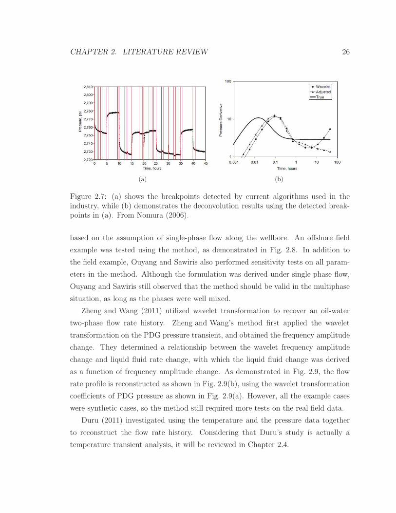
PDG data analysis, especially in the calculation of deconvolution. Nomura (2006)
determined that a breakpoint inaccuracy that could not even be detected with hu-
man eyes still led to huge deviation in the deconvolution results. As shown in Fig-
ure 2.7, the breakpoint detection (Fig. 2.7(a)) using the current commercial algo-
rithm from Athichanagorn (1999) seems good visibly, but the deconvolution result
(Fig. 2.7(b)) based on this breakpoint detection deviates substantially from the true
answer.
Nomura’s examples illustrate the industrial demand for the high level accuracy in

CHAPTER 2. LITERATURE REVIEW 25
Figure 2.6: Breakpoint detection using both the pressure and the flow rate data.Most visually apparent breakpoints are detected, but still some are missed. From Rai(2005).
breakpoint detection. Nowadays, researchers and engineers are still working on the
accurate breakpoint detection. In this dissertation, both the methods with breakpoint
detection and the methods without breakpoint detection will be discussed. Providing
a method that does not require breakpoint detection is a clear advantage.
2.2.3 Flow Rate Reconstruction
As the early PDG tools did not provide the downhole flow rate information, the
pressure data has been used to reconstruct the flow rate series. This approach is
still often used today, as PDGs that measure both pressure and flow rate are now
available, but are deployed relatively infrequently.
Ouyang and Sawiris (2003) raised the question of reconstructing the production
and injection flow rate profile using the PDG pressure data. In their work, a key
numerical solution of flow rate as the function of downhole pressure was derived,
CHAPTER 2. LITERATURE REVIEW 26
(a) (b)
Figure 2.7: (a) shows the breakpoints detected by current algorithms used in theindustry, while (b) demonstrates the deconvolution results using the detected break-points in (a). From Nomura (2006).
based on the assumption of single-phase flow along the wellbore. An offshore field
example was tested using the method, as demonstrated in Fig. 2.8. In addition to
the field example, Ouyang and Sawiris also performed sensitivity tests on all param-
eters in the method. Although the formulation was derived under single-phase flow,
Ouyang and Sawiris still observed that the method should be valid in the multiphase
situation, as long as the phases were well mixed.
Zheng and Wang (2011) utilized wavelet transformation to recover an oil-water
two-phase flow rate history. Zheng and Wang’s method first applied the wavelet
transformation on the PDG pressure transient, and obtained the frequency amplitude
change. They determined a relationship between the wavelet frequency amplitude
change and liquid fluid rate change, with which the liquid fluid change was derived
as a function of frequency amplitude change. As demonstrated in Fig. 2.9, the flow
rate profile is reconstructed as shown in Fig. 2.9(b), using the wavelet transformation
coefficients of PDG pressure as shown in Fig. 2.9(a). However, all the example cases
were synthetic cases, so the method still required more tests on the real field data.
Duru (2011) investigated using the temperature and the pressure data together
to reconstruct the flow rate history. Considering that Duru’s study is actually a
temperature transient analysis, it will be reviewed in Chapter 2.4.

CHAPTER 2. LITERATURE REVIEW 27
(a)
(b)
Figure 2.8: Using the pressure profile as shown in (a), the flow rate profile is recon-structed as shown in (b). From Ouyang and Sawiris (2003).

CHAPTER 2. LITERATURE REVIEW 28
(a)
(b)
Figure 2.9: Using the wavelet transformation coefficients of PDG pressure as shownin (a), the flow rate profile is reconstructed as shown in (b). From Zheng and Wang(2011).

CHAPTER 2. LITERATURE REVIEW 29
Although the modern permanent downhole gauges have already achieved the ca-
pability of downhole flow rate measurement, better flow rate reconstruction methods
are still needed because many permanent downhole gauges that cannot measure the
flow rate are still deployed. Moreover, PDG data sets with partially missing flow rate
are also very common. Accurate flow rate reconstruction methods will be very helpful
in these cases.
2.2.4 Change of Reservoir Properties
The fact that the reservoir properties change during production has been noticed
for a long time. Lee (2003) demonstrated history matching to a two year record
of pressure, as shown in Fig. 2.10. The pressure simulation result with variable
permeability and skin overwhelmingly beats that with constant reservoir properties.
Unlike the conventional well tests which only use measurements of short duration,
PDGs may provide long-term measurements. The long-term PDG data, therefore,
are expected to be affected by the change in the reservoir properties or behavior.
Figure 2.10: A comparison between the pressure history matching with constant andvariable reservoir properties, from Lee (2003).
Dealing with the reservoir property change, Lee (2003) estimated the permeabil-
ity and the skin factor as functions of time. Regressing on the parameters of the

CHAPTER 2. LITERATURE REVIEW 30
functions (simulations were performed in each iteration), the estimation of the reser-
voir properties is shown in Fig. 2.11. These estimations made by Lee were all based
on the assumption that the reservoir properties are functions of time only. Actually
the reservoir properties may also be affected by other factors, such as the change
of reservoir flow mechanisms. Nevertheless assuming the properties are functions of
time only could be treated as a convenient model to accommodate all the factors.
Figure 2.11: Estimate the permeability as a quadratic function of time, and the skinfactor as a linear function of time, from Lee (2003).
For the same PDG data, Khong (2001) has made a further investigation of the
moving window method proposed by Athichanagorn (1999). Khong set a width of a
window, and moved the window slowly with a predefined interval from the begging
of the data set till the end. Transient analysis was applied to each window, thus
yielding a series of reservoir properties as a function of time. Fig. 2.12 showed the
permeability change using the moving window method. The moving window method
was also used in Athichanagorn et al. (2002).
Zheng and Li (2007) also used a window-like method. In Zheng and Li’s study,
they first applied wavelet method to detect breakpoints and to define transients. In
each transient, they assumed the reservoir properties were constant. The result is a
sequence of piecewise constant reservoir properties, such as the permeability and the
skin factor shown in Fig. 2.13.

CHAPTER 2. LITERATURE REVIEW 31
Figure 2.12: Variable permeability obtained by the moving window method on thePDG pressure data, from Khong (2001).
Figure 2.13: Piecewise constant reservoir properties after transient analysis,from Zheng and Li (2007).

CHAPTER 2. LITERATURE REVIEW 32
2.3 Deconvolution
As some modern PDG devices have the capability of flow rate measurement, the
cointerpretation of pressure and flow rate data from the PDG, rather an analysis on
the pressure data only, has gained attention. Beyond the use specifically for PDG
data analysis, a common pressure/flowrate cointerpretation method is deconvolution.
Deconvolution is the process that uses the pressure transient response to variable
flow rate to compute the corresponding constant flow rate response. As expressed in
Eq. 2.4, the wellbore pressure drop, ∆pw (t) can be constructed by the convolution
of individual constant rate transient, ∆p0 (t). Therefore, the deconvolution process is
to extract the constant flow rate transient ∆p0 (t), from the convolved variable rate
transients, ∆pw (t).
∆pw (t) =
∫ t
0
q′ (t) ·∆p0 (t− τ) dτ (2.4)
Deconvolution has been discussed for decades, with most approaches being analyt-
ical. For example, Ramey (1970) applied Laplace transform on the pressure diffusion
equation to solve the partial differential equation in the Laplace space. However, ap-
plying the deconvolution to the numerical measurement from PDGs was not practical
until a series of important work by von Schroeter et al. (2004). The difficulty is that
the deconvolution process is actually a “desmoothing” process (Horne, 2007), because
the forward convolution equation (Eq.2.4) is a smoothing function. This “desmooth-
ing” process brings in serious instability issue in the mathematical solution, especially
when the data are noisy.
von Schroeter et al. (2004) made important breakthroughs by proposing a formu-
lation that enables solving the deconvolution problem as a separable nonlinear Total
Least Squares problem, and applied this algorithm to PDG data. A multitransient
simulated example was demonstrated in their work, as shown in Fig. 2.14. The dashed
curve is the deconvolution result, while the black and the grey dots are true and noisy
data. von Schroeter et al. had developed a method by which the feasible and stable
deconvolution process may be carried out.
Levitan et al. (2006) described a deconvolution technique using an unconstrained

CHAPTER 2. LITERATURE REVIEW 33
(a) (b)
Figure 2.14: Deconvolution applied on the (a) variable flow rate and (b) multipletransients.The dashed curve is the deconvolution result, while the black and the greydots are true and noisy data, from von Schroeter et al. (2004).
objective function constructed by matching pressure and pressure derivative generated
by the response functions derived from different pressure build-up (PBU) periods.
One successful application of their method is to recover the initial pressure. According
to their work, the initial reservoir pressure may be regressed until convolution results
in two or more PBUs converge, as illustrated in Fig. 2.15. This method was proven to
be effective when the flow rate history is simple and the flow rate data are accurate
especially when the breakpoints of the flow rate are identified accurately.
Ahn and Horne (2008) proposed another deconvolution method using convex op-
timization approaches. The method permits the existence of noise in both pressure
and flow rate data and the accuracy of the deconvolution is assured by the iterative
convex optimization process. The method was successful on real field data, as shown
in Fig. 2.16. However, the method does not perform well if a buildup transient was
not fully developed in the deconvolution range. Especially when the data set is short
(not enough for a full transient) and noisy, the method will not work.
Most current deconvolution algorithms require breakpoint detection in advance.
As discussed earlier, the breakpoint detection with high level accuracy is a challenge.
As discussed in Section 2.2.2, Nomura (2006) showed that a tiny miss in break point
detection may result in a huge deviation in the deconvolution result(Fig. 2.7(a)). The
instability of deconvolution algorithms, and the difficulty in the high level accurate

CHAPTER 2. LITERATURE REVIEW 34
(a)
(b)
Figure 2.15: (a) Using the initial reservoir pressure of 6310 psi leads to the in-convergence of the deconvolution results on two PBUs. (b)However, with the initialreservoir pressure of 6314.3 psi deconvolution results on two PBUs converged witheach other, from Levitan et al. (2006).

CHAPTER 2. LITERATURE REVIEW 35
(a) (b)
Figure 2.16: Deconvolution using the convex optimization on the real filed data: (a)shows the pressure matching after four iterations, and (b) shows the flow rate match-ing after four iteration, from Ahn and Horne (2008).
breakpoint detection are the two prime difficulties of deconvolution of PDG data.
Nevertheless, the insights of the reservoir that would be brought by a successful de-
convolution process are still irreplaceable in the PDG data analysis domain. Actually,
the second target of this study, stated in Section 1.1 may obtain similar results of
deconvolution. The detailed discussion will appear in later chapters.
2.4 Temperature Transient Analysis
Downhole temperature measurement by permanent downhole temperature gauges has
been available as early as the initial development of PDGs. However, unlike the pres-
sure data that have been widely and deeply studied, the usage of PDG temperature
measurements still remains mostly for well monitoring. For example, Kragas et al.
(2004) demonstrated an example of downhole pressure and temperature from PDGs
synchronized with the well events (Fig. 2.17). The events, such as perforation, may
be clearly reflected in the pressure change as well as in the temperature change.
Fig. 2.17 actually shows another important relation behind the curves, that the
temperature also has transient behavior corresponding to the flow rate change, anal-
ogous to that of pressure. This inspires people working on temperature transient

CHAPTER 2. LITERATURE REVIEW 36
Figure 2.17: Real time downhole temperature and pressure data from PDG synchro-nized with the well events, from Kragas et al. (2004).
analysis.
Some fundamental work of temperature transient analysis has been achieved
in Duru and Horne (2010, 2011). Duru and Horne (2010) derived a temperature tran-
sient model as a function of fluid properties, formation parameters, pressure, and
flow rate. The model related the mass balance and the energy balance by the
Joule-Thomson effect and the heat diffusion effect. Duru and Horne (2011) applied
Bayesian inversion method in solving the temperature transient model derived in
Duru and Horne (2010). The Bayesian inversion method is stochastic and power-
ful. The method deconvolves variable-rate pressure data and extracts the pressure
response kernel function. The method may even recover the flow rate history from
the variable-rate temperature data. The method has a good tolerance of noise, that
is, even with 10% noise, the method still works well. Fig. 2.18 shows a case of tem-
perature and pressure transient analysis using the temperature model and Bayesian
inversion method. The pressure response kernel function (Fig. 2.18(b)) was extracted
from the pressure data with 10% noise (Fig. 2.18(a)), while the flow rate history
(Fig. 2.18(d)) was recovered from the temperature data (Fig. 2.18(c)).

CHAPTER 2. LITERATURE REVIEW 37
(a) (b)
(c) (d)
Figure 2.18: Temperature and pressure transient analysis with Bayesian inversionmethod. (a) the pressure data with 10% noise; (b) the extracted pressure responsekernel function from the noisy pressure data; (c) the temperature data and the repro-duced temperature; (d) the recovered flow rate history from the temperature data,from Duru and Horne (2011).

CHAPTER 2. LITERATURE REVIEW 38
Temperature is not the main focus of this study. However, temperature data are
another important data source for the reservoir characterisation. It could be very help-
ful that the current study retained some flexibility and extendability to incorporate
the cointerpretation using the pressure, flow rate, and temperature simultaneously.
This flexibility and extendability requires some perspective insights on the high level
architecture design of the method.
2.5 Data Mining
One of the fundamental properties of PDG data is the large number of data points.
This property associates the PDG data exploration with an idea from the computer
science domain, data mining. Data mining is a process to extract models from large
volumes of data. It seems promising to use data mining in the processing of PDG
data. Assuming the PDG data reflect the properties of the reservoir, proper data
mining algorithms may be able to extract the reservoir model from the PDG data
despite them being variable and noisy. However, up to now, few attempts to apply
data mining to PDG data have been made.
Liu (2009) proposed a data mining method applied on the pressure transient in
the Laplace space. The method first transformed all the PDG data from the real
time space to the Laplace space, then applied a data mining process, namely Locally
Weighted Projection Regression, on the transformed pressure transient in the Laplace
space, and finally inverted the prediction of the data mining process from the Laplace
space to the real time space. Fig. 2.19 shows a synthetic case, comparing the pressure
prediction after data mining in the Laplace space, the original noisy data, and the
underlying synthetic true data. Considering that the synthetic true data is invisible
to the data mining process, and that all that the data mining algorithm could see
are the noisy data, the prediction is good. Fig. 2.20 shows the result of a real field
case, in which the real pressure is unknown. Compared with Fast Fourier Transform
or wavelet methods which smooth and filter the data, the method removes the larger
noise of the PDG data while preserving the local variations. These local variations
may contain useful information from the subsurface rather than being just noise.

CHAPTER 2. LITERATURE REVIEW 39
0
100
200
300
400
500
600
700
800
0 100 200 300 400 500 600
Pres
sure
Time(samples)
Prediction from LWPR in Laplace Space
True DataNoisy DataPrediction
(a)
400
450
500
550
600
30 35 40 45 50 55 60 65 70
Pres
sure
Time(samples)
Prediction from LWPR in Laplace Space
True DataNoisy DataPrediction
(b)
Figure 2.19: Pressure prediction in the real space after data mining in the Laplacespace. (a) shows the pressure prediction compared with the noisy and synthetic truedata; (b) shows a zoom-in view of the pressure prediction (Liu, 2009).
-0.2
-0.1
0
0.1
0.2
0.3
0.4
0.5
0.6
0.7
0.8
0 50 100 150 200 250
Pres
sure
Time(samples)
Prediction from LWPR in Laplace Space
Real DataPrediction
Figure 2.20: Pressure prediction on real data after data mining in Laplace space (Liu,2009).

CHAPTER 2. LITERATURE REVIEW 40
The reason that Liu (2009) chose to perform the data mining process in the
Laplace space is because the pressure transients are convolved in the real time space
and they could be deconvolved easily in the Laplace space. However, Liu (2009) had a
difficulty that more than 40% of computational time was spent on the transformation
and inversion between the real time space and the Laplace space. A data mining
method applied directly in the real time space would be more desirable. Therefore,
a fundamental target of the current study was that all the data mining algorithms
should work directly in the real time space.

Chapter 3
Data Mining Concept and Simple
Kernel
Data mining is a technique that is widely used in computer science. It is the process
of extracting patterns from data, and it plays a key role in many areas of science,
finance and industry. There are some examples of data mining described earlier in
Section 1.2.
Data mining commonly involves two main classes of tasks, regression and classi-
fication. Regression attempts to solve the continuous-solution problems by finding a
function to model the data with least error. In regression problems, the output is a
continuous physical or mathematical variable. For example, in the stock price predic-
tion problems, the regression output is the predicted stock price that is continuous.
Classification intends to solve the discrete-solution problems by categorizing the data
into different groups with least misclassification. In classification problems, the out-
put is a discrete group label and usually has no physical or mathematical meanings.
For example, in the spam email classification problems, the output is binary, 0 or 1
that represents the email is a spam email or a nonspam email.
There are two major classes of data mining algorithms, supervised learning and
unsupervised learning. The supervised learning is based on training data set. For
each training sample in the training data set, an input and an output will be provided.
The supervised learning algorithm aims to find the general correlation between the
41

CHAPTER 3. DATA MINING CONCEPT AND SIMPLE KERNEL 42
input and the output by being trained by all the samples in the training data set.
Take the spam mail case as an example. Usually people provide an email database as
the training data set. In the training data set, each email and corresponding spam-
indicator (0 for a spam email and 1 for a nonspam email) form a training sample
in which the email is an input, and the spam-indicator is an output. After being
trained by all the samples in the training data set, the supervised learning algorithm
is assumed to obtain the relationship between the email and the spam-indicator, such
that whenever a new email is received, the learning algorithm may be able to give a
spam-indicator prediction to predict whether this email is a spam email or not. As
the training data set performs as a guide or a teacher to the data mining algorithm,
the supervised learning is also named learning with a teacher.
The opposite of the supervised learning, the unsupervised learning is often called
learning without a teacher. In an unsupervised learning algorithm, there is no
training data set provided. The unsupervised learning is assumed to work directly
on a data set and infer the relationships or properties among the variables in the
data set. The case of association rule makes a good demonstration that the unsuper-
vised learning digs into the transaction data set finding out that 80% of supermarket
customers who buy beer also buy chips.
The data mining problem in this study is mainly a supervised regression problem.
The PDG data are used to construct the training data set, and the data mining
algorithm predicts the pressure as the function of flow rate and time. There is also
a study regarding the breakpoint detection via data mining approaches, described in
the appendix. That problem is an unsupervised classification problem in which the
data mining algorithm groups the PDG data points into transients.
3.1 Components of Learning Algorithm
In a data mining algorithm, there are three important components, including model,
cost function, and optimization search method. They are the core parts of a learning
algorithm, so a brief introduction of them is given here.

CHAPTER 3. DATA MINING CONCEPT AND SIMPLE KERNEL 43
3.1.1 Model
The model serves as the pattern structure or underlying functional form sought from
the data. A model reflects the pattern structure of the observed data, and may also
provide the prediction given any predefined inputs, shown in Equation 3.1.
ypred = hθ (x) (3.1)
where, x = (x1, x2, . . . , xNx)T in general is the input vector of the input values. Nx
is the number of elements of each input vector. The element of the input vector is
also called the “feature”.hθ : RNx → R is a model, which in general is a nonlinear
function. θ = (θ1, θ2, . . . , θNθ)T is a vector of model parameters. Nθ is the number of
model parameters. ypred is the prediction by the hypothesis hθ (x) at x. In this study
θ will have no physical meaning and is needed only to train the algorithm.
In a few cases, the pattern of the data is known before data mining. People
may use the known pattern structure as the model. For example, in some seismic
studies, the forward model is known, and thus, the forward model may be used as the
model for the data mining. However, the pattern structure of the data is unknown in
most cases. In this situation, the model is a pattern structure proposed intuitively or
intentionally. Because complex models always lead to intensive computation, a linear
model is often the first choice. Thus for the case of PDG data model, as a preliminary
investigation (only) we could use a linear model as expressed in Eq. 3.2.
hθ (x) = θTx = 〈θ,x〉 (3.2)
where 〈·, ·〉 is the inner product of two vectors. θ = (θ1, θ2, . . . , θNx)T is a vector of
model parameters with the same size as input vector x.
For PDG data, studied in this work, the input vector is defined throughout this
and the next section as:
x(i) =
x(i)1
x(i)2
x(i)3
=
1
q(i)
t(i)
, i = 1, . . . , Np (3.3)

CHAPTER 3. DATA MINING CONCEPT AND SIMPLE KERNEL 44
where Np is a number of the observed (measured) pressures, t(i) is the time point at
which ith pressure was measured, q(i) is the flow rate at time t(i) and a constant value
1. The existence of the constant “1” is to make the linear expression cover a possible
offset. The model will predict the values ypred(i), which in fact are the predicted
pressures ppred(i) at time t(i), where the PDG pressures were measured. Thus the
model for PDG data is:
ypred(i) = θTx(i), i = 1, . . . , Np (3.4)
where the model parameter vector is:
θ =
θ1
θ2
θ3
(3.5)
The observed data are the pressures measured at time t(i), namely p(i):
yobs(i) = p(i), i = 1, . . . , Np (3.6)
When a model is provided, the data mining question actually becomes an opti-
mization question to determine values of θ to be used to have the best fit of the
data.
3.1.2 Cost Function
A cost function judges the quality of the model compared to the acquisition data,
denoted as L(
ypred, yobs)
. Here, ypred is the prediction from the model, as stated in
Eq. 3.1, and yobs is the observation, y(i). Considering the model ypred = hθ (x) is also
a function of θ given the input data x. Essentially the cost function is a function of
θ, such that L = L (θ). This reveals the essence of a cost function as an evaluation of
the parameter vector θ. In this study, the least-mean-square (LMS) is employed as

CHAPTER 3. DATA MINING CONCEPT AND SIMPLE KERNEL 45
shown in the Eq. 3.7
LLMS (θ) =1
2
Np∑
i=1
(
hθ
(
x(i))
− y(i))2
(3.7)
The LMS cost function emphasizes the fitting of the model to the observed data.
However, it tends to have very complex parameters θ which results in overfitting of
the data. A better way to restrain θ is to have a penalty term in the cost function,
shown in Equation 3.8.
LMAP (θ) =1
2
Np∑
i=1
(
hθ
(
x(i))
− y(i))2
+ c ‖θ‖ (3.8)
The cost function in Equation 3.8 is also called Maximum A Posteriori (MAP)
(Koller and Friedman, 2009) cost function. When the vector θ is too complex, ‖θ‖,the norm of the θ becomes larger. Also the cost will be increased by a penalty
coefficient. So the MAP cost function actually restrains the models on both the data
fitting and the model structure. The weight between the two is controlled by the
coefficient c.
When the model of a data mining is fixed, the cost function needs careful selection
to regularize the model in an expected way. In this work, LMS cost function was
taken. Here the LMS was chosen as the cost function not only because its simplicity.
If the data mining model is linear, the LMS cost function will be a convex function
whose Hessian Matrix is positive-definite, that is, the cost function will have only
one global minimum and there is no other local minimum at all. This property
is very useful in the data mining, because it releases the optimization method from
choosing a very good initial guess that has to be very close to the global minimum.
To prove the LMS cost function is a convex function, we may examine the element
(p, q) of the Hessian Matrix (H) of L (θ), which is:
Hpq =∂2
∂θp∂θqL (θ) =
Np∑
i=1
x(i)p x(i)
q (3.9)

CHAPTER 3. DATA MINING CONCEPT AND SIMPLE KERNEL 46
Then for any vector z,
zTHz =
Nθ∑
p=1
Nθ∑
q=1
zpzqHpq
=
Nθ∑
p=1
Ntheta∑
q=1
zpzq
Np∑
i=1
x(i)p x(i)
q
=
Np∑
i=1
Nθ∑
p=1
Nθ∑
q=1
zpzqx(i)p x(i)
q
=
Np∑
i=1
((
Nθ∑
p=1
zpx(i)p
)(
Nθ∑
q=1
zqx(i)q
))
=
Np∑
i=1
(
Nθ∑
p=1
zpx(i)p
)2
>0 (3.10)
The derivation in Eq. 3.10 shows the Hessian matrix in Eq. 3.9 is positive-definite.
3.1.3 Optimization Search Method
The optimization search method minimizes the cost function. Any data mining algo-
rithm requires minimization of the cost function to a global minimum robustly and
efficiently. There are generally two kinds of optimization methods, gradient-based and
not gradient-based. The gradient-based methods are usually very fast, like Steepest
Gradient Descent methods, Conjugate Gradient Descent, etc. In early stages of this
research, the Steepest Gradient Descent method was used. The gradient descent
method starts from an initial guess, and performs updates repeatedly as shown in
Eq. 3.11.
θ[i+1]j = θ
[i]j − α
∂
∂θjL (θ) = θ
[i]j − α
Np∑
k=1
(
hθ[j](
x(k))
− y(k))
x(k)j (3.11)

CHAPTER 3. DATA MINING CONCEPT AND SIMPLE KERNEL 47
here α is the learning rate which is chosen a proper value by experience1 and [m] is
the mth iteration.
Eq. 3.11 could be realized by the Batch Gradient Descent algorithm, as shown by
pseudocode in Algorithm 1. Actually, this is too expensive computationally, especially
when the training data set is very large. Also, it is not necessary to use the whole data
set to do the training in a single update step because it is very possible that θ has
converged before the whole data set is applied. Therefore, a better way to implement
the gradient descent method is to use Stochastic Gradient Descent algorithm, as
shown by pseudocode in Algorithm 2. In the Stochastic Gradient Descent algorithm,
each time θ is updated by a single sample only. The training is processed repeatedly
until θ has converged.
Algorithm 1 Batch Gradient Descent
iter = 0 initialize the iteration counterθ[0] = ~0 initial guess of θwhile θ[iter] is not converged doθ[iter+1] = θ[iter]
for i = 1 to Np do
θ[iter+1] = θ[iter+1] − α(
hθ
(
x(i))
− y(i))
x(i) Update θ by all samplesend foriter = iter + 1 update the iteration counter
end while
With the Stochastic Gradient Decent method, the training process in Eq. 3.11
may be simplified into Eq. 3.12.
θ[i+1]j = θ
(0)j − α
i∑
k=0
(
hθ[k](
x(k+1))
− y(k+1))
x(k+1)j (3.12)
1α does not have fixed range. A large α will lead to a fast convergence at the beginning and azigzag oscillation at the end, which very possible leads to an nonconvergence; however, a small αcan improve the convergence at the end but it converges very slowly at the beginning. A properstrategy to select the α is trial-and-error. In the coming chapters, the Conjugate Gradient methodwill replace the current Steepest Gradient Descent method to accelerate the convergence rate as wellas avoid the tricky selection of α. This is described later, in Section 4.3

CHAPTER 3. DATA MINING CONCEPT AND SIMPLE KERNEL 48
Algorithm 2 Stochastic Gradient Descent
iter = 0 initialize the iteration counterθ[0] = ~0 initial guess of θwhile θ[iter] is not converged doi = ((iter + 1) mod Np) + 1
θ[iter+1] = θ[iter] − α(
hθ
(
x(i))
− y(i))
x(i) Update θ iter = iter + 1
end while
If we make an initial guess of θ[0] as 0, then Eq. 3.12 will be simplified as Eq. 3.13.
θ[i+1]j = α
i∑
k=0
(
y(k+1) − hθ[k](
x(k+1)))
x(k+1)j (3.13)
Eq. 3.13 is the training equation of the learning process. According to the model
we selected, the prediction equation will be written easily as Eq. 3.14, where xpred is
a given input which the prediction is required to make.
ypred = hθ
(
xpred)
= θTxpred (3.14)
In a supervised learning process, the cost function is a function of the parameters
θ and the training data. The optimization process is a process of obtaining the best
θ through utilizing the training data set to minimize the cost function. The process
looks like using the training data set to train the model parameter θ. This is where
the word “train” originates.
With these three components, a data mining algorithm could be performed, that
is, given a model and a cost function, a proper optimization method may find the
best parameters in the model to produce the least cost. Now that the whole data
mining process has been discussed, it is appropriate to discuss some of its problems.
The model proposed in this section is the most generic linear model. The difficulty of
proposing this model is that we force the pattern structure behind the PDG data to
be linear, or in other words, the model only captures the linearity of the PDG data.
However it is well understood that the PDG data are nonlinear at the large scale,
as shown in Fig. 1.3. Apparently from the curve, it may be seen that the pressure

CHAPTER 3. DATA MINING CONCEPT AND SIMPLE KERNEL 49
transient is not related to the flow rate in a linear manner. Essentially, the pressure
transient is the convolution results of flow rate change events, which means that each
pressure is affected by all previous flow rate events starting at different time. Because
the nonlinearity is dominant throughout the whole duration of the PDG data, failing
to capture the nonlinearity will lead to failure to obtain the reservoir model, and
ultimately will fail to give a correct interpretation of the PDG data. So the question
becomes how to capture the nonlinearity with a linear model in the data mining
process.
3.2 Kernelization
An easy way to capture the nonlinearity by a linear model is to use a transformation
on the input vector x. For example, suppose the actual pattern structure behind the
data pair (y, z) is y = θ1 + θ2z + θ3z2, and suppose the model is linear as y = θTx. If
x is defined as:
x =
(
1
z
)
(3.15)
then in this two-dimensional space of of (1, z)T, the linear model hθ (x) = θTx will
only capture the linearity of y, and the second-order nonlinearity z2 could not be
captured. However, if there exist a transformation Φ (x) over vector x such that:
Φ (x) :
(
1
z
)
→
1
z
z2
(3.16)
Then in this three-dimensional space of (1, z, z2)T, the linear model hθ (x) = θTΦ (x)
will capture the quadratic nonlinearity of y. This example reveals that the nonlinearity
in a low-dimensional space could be approached by the linearity in a high-dimensional
space. The Φ (x) here is just a general form of transformation over vector x. We
actually do not know the dimension of Φ (x). It may be more than Nx, may be less,
and may be equal. Considering that we would like to capture more nonlinearity by

CHAPTER 3. DATA MINING CONCEPT AND SIMPLE KERNEL 50
imposing Φ (x), the dimension of Φ (x) will be mostly more than Nx. In the example
in Eq. 3.16, the dimension of Φ (x) is three, which is greater than the dimension of x.
Correspondingly, the dimension of θ will be the same as that of Φ (x), rather than
that of θ. To make clear, θ has the same dimension as x before Eq. 3.16, while θ has
the same dimension as Φ (x) after Eq. 3.17.
Therefore, we may slightly modify Eq. 3.13 and Eq. 3.14 to reflect this transfor-
mation. The input variable x is replaced by Φ (x). The training equation becomes:
θ[i+1]j = α
i∑
k=0
(
y(k+1) − hθ[k](
Φ(
x(k+1))))
Φ(
x(k+1)j
)
(3.17)
and the prediction equation becomes:
ypred = hθ
(
Φ(
xpred))
= θTΦ(
xpred)
(3.18)
This form of the model (Eq. 3.17 and Eq. 3.18) will capture different nonlin-
earities according to different selections of the transformation. For the case dis-
cussed, to capture the nonlinearity of a p-degree polynomial, a transformation of
Φ (x) = (1, z, z2, . . . , zp)Thas to be constructed explicitly. This brings in another
problem that the more nonlinearity we would like to catch, the more complex the
transformation Φ (x) will be, and the more computation would be required. Another
difficulty is that we may not know the relevant functional form from Φ (x) in advance.
It is very natural to ask “is it possible that we construct Φ (x) without writing Φ (x)
out explicitly?”
If we multiply Eq. 3.17 by Φ(
x(i+2))
, we have:

CHAPTER 3. DATA MINING CONCEPT AND SIMPLE KERNEL 51
θ[i+1]TΦ(
x(i+2))
=αi∑
k=0
(
y(k+1) − hθ[k](
Φ(
x(k+1))))
Φ(
x(k+1))T
Φ(
x(i+2))
=α
i∑
k=0
(
y(k+1) − θ[k]TΦ(
x(k+1))
)
Φ(
x(k+1))T
Φ(
x(i+2))
=α
i∑
k=0
(
y(k+1) − θ[k]TΦ(
x(k+1))
)
⟨
Φ(
x(k+1))
,Φ(
x(i+2))⟩
=α
i∑
k=0
(
y(k+1) − θ[k]TΦ(
x(k+1))
)
K(
x(k+1),x(i+2))
(3.19)
Finally, we write out the new form of training equation as
θ[i+1]TΦ(
x(i+2))
= α
i∑
k=0
(
y(k+1) − θ[k]TΦ(
x(k+1))
)
K(
x(k+1),x(i+2))
(3.20)
Here, K (x, z) is named the kernel function, defined by the inner product of the
transformations shown in Eq. 3.21.
K (x, z) = 〈Φ (x) ,Φ (z)〉 (3.21)
Although the Kernel function is defined by the inner products of (x), it usually
does not require the explicit formation of Φ (x) to make the computation. Assume
x = (x1, x2, x3)T and z = (z1, z2, z3)
T, two classical kernel functions and their cor-
responding Φ (x) are shown in Table 3.1. The first kernel function maps x from
three-dimensional space onto nine-dimensional space Φ (x), while the second kernel
function maps onto 13-dimensional space. Although the two Φ (x) in the table are
in high-dimensional spaces, the calculations of K (x, z) are both done in the three-
dimensional space, which significantly improves the performance. This demonstrates
that the kernel function may realize transformation onto a high-dimensional space
with the calculation in the low-dimensional space.
The proof of the first correlation between the kernel function K (x, z) and the
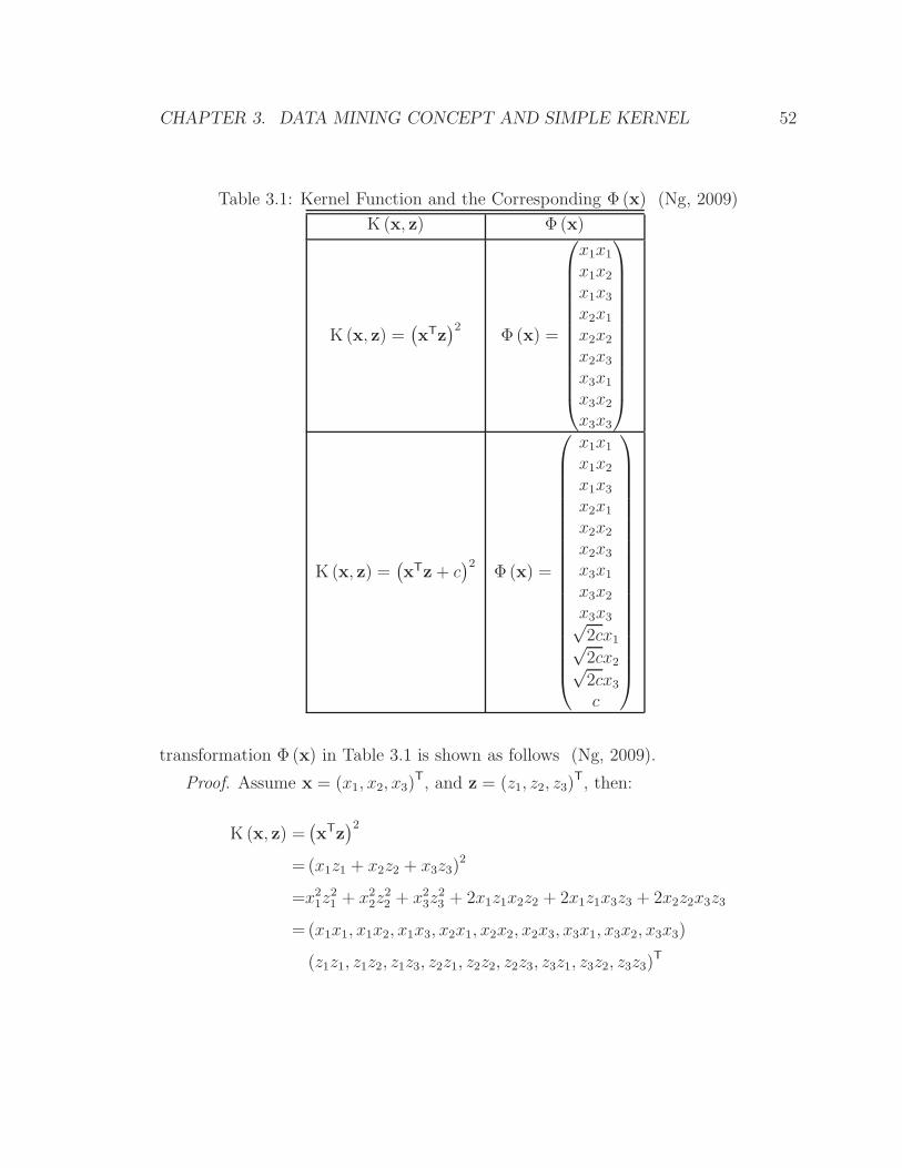
CHAPTER 3. DATA MINING CONCEPT AND SIMPLE KERNEL 52
Table 3.1: Kernel Function and the Corresponding Φ (x) (Ng, 2009)
K (x, z) Φ (x)
K (x, z) =(
xTz)2
Φ (x) =
x1x1
x1x2
x1x3
x2x1
x2x2
x2x3
x3x1
x3x2
x3x3
K (x, z) =(
xTz+ c)2
Φ (x) =
x1x1
x1x2
x1x3
x2x1
x2x2
x2x3
x3x1
x3x2
x3x3√2cx1√2cx2√2cx3
c
transformation Φ (x) in Table 3.1 is shown as follows (Ng, 2009).
Proof. Assume x = (x1, x2, x3)T, and z = (z1, z2, z3)
T, then:
K (x, z) =(
xTz)2
=(x1z1 + x2z2 + x3z3)2
=x21z
21 + x2
2z22 + x2
3z23 + 2x1z1x2z2 + 2x1z1x3z3 + 2x2z2x3z3
=(x1x1, x1x2, x1x3, x2x1, x2x2, x2x3, x3x1, x3x2, x3x3)
(z1z1, z1z2, z1z3, z2z1, z2z2, z2z3, z3z1, z3z2, z3z3)T

CHAPTER 3. DATA MINING CONCEPT AND SIMPLE KERNEL 53
Considering K (x, z) = Φ (x)T Φ (z), we have:
Φ (x) = (x1x1, x1x2, x1x3, x2x1, x2x2, x2x3, x3x1, x3x2, x3x3)T
and:
Φ (z) = (z1z1, z1z2, z1z3, z2z1, z2z2, z2z3, z3z1, z3z2, z3z3)T
Here we show that when we use the kernel function K (x, z) =(
xTz)2, we are
implicitly using Φ (x) = (x1x1, x1x2, x1x3, x2x1, x2x2, x2x3, x3x1, x3x2, x3x3)T. This
enables us to make the calculation in three-dimensional space (the space of vector x),
while run the learning algorithm in the nine-dimensional space (the space of Φ (x)).
However, although the kernel function only evaluates on vector x and z, not all
functions evaluating on x and z are valid kernel functions. A valid kernel is also called
a Mercer kernel, because Mercer developed criteria for the kernel validity, namely the
Mercer Theorem.
Mercer Theorem (Ng, 2009). Let K : ℜn × ℜn → ℜ be given. then for K to be a
valid (Mercer) kernel, it is necessary and sufficient that for any
x(1), . . . ,x(m)
, m <
∞, the corresponding kernel matrix K is symmetric positive semi-definite, where a
kernel matrix K is defined so that its (i, j)-entry is given by Kij = K(
x(i),x(j))
.
By using these “kernel tricks” although Eq. 3.20 involves Φ (x), it does not require
Φ (x) to be written out explicitly. The term θ[k]TΦ(
x(i+2))
is a recurrent term on the
left hand side of Eq. 3.20, which is calculated and stored in the previous iterations.The⟨
Φ(
x(k+1))
,Φ(
x(i+2))⟩
term is replaced by a kernel function K(
x(k+1),x(i+2))
which
is expressed by x(k+1) and x(i+2) instead. Therefore, Eq. 3.20 makes the calculation
using Φ (x) implicitly. In practice, for well test data interpretation, this means that
we match the measured data without knowing in advance what the reservoir model
is – in fact, the reservoir model is discovered in the process.
Similarly, the prediction equation, Eq. 3.18, becomes:
ypred = hθ
(
Φ(
xpred))
=
Niter∑
k=0
α(
y(k+1) − θ[k]TΦ(
x(k+1))
)
K(
x(k+1),xpred)
(3.22)

CHAPTER 3. DATA MINING CONCEPT AND SIMPLE KERNEL 54
where Niter is the total number of the iterations before convergence. Usually Niter is
larger than Np because the training data will be used repeatedly before θ converges.
Even though there is a term of θ[k]TΦ(
x(k+1))
in Eq. 3.22, the equation still does not
require us to know Φ (x) explicitly. This is because the term θ[k]TΦ(
x(k+1))
is the
recurrent term stored during the training process (the left hand side of the training
equation, Eq. 3.20). So we do not have to know Φ (x) at all.
Eq. 3.20 and Eq. 3.22 kernelize the linear model with a kernel function enabling
the data mining algorithm to capture the nonlinearity using a linear model with
the calculation still in low-dimensional space. This process is named “kernelization”.
With the kernelized data mining algorithm, we are able to formulate different methods
to perform data mining on the PDG data. Those methods may be classified into two
categories, kernelized data mining without breakpoint detection, and kernelized data
mining with breakpoint detection. These will be discussed separately in the following
sections.
3.3 Kernelized Data Mining without Breakpoint
Detection
The reservoir response is controlled by a linear combination due to superposition of
individual flow rate responses. Fig. 3.1 demonstrates the formation of the superposi-
tion. Assume there are two flow rates q1 and q2 starting at different time. When either
of them appears individually, the reservoir will respond with pressure changes p1 and
p2 respectively. When they appear together, the flow rates will be combined, shown in
the figure as a constant flow rate followed by a zero flow rate. The pressure responses
are also summed up so that the pressure curve behaves as a drawdown followed by a
buildup. What is observed by the PDG is the combination result after superposition.
In fact, it will be much easier for the data mining algorithm to converge if trained
with separated constant flow rate and corresponding pressure responses. Therefore,
it will be very beneficial if the real breakpoints, where the real flow rate change events
happen, could be detected. However, considering the flow rate and pressure signals

CHAPTER 3. DATA MINING CONCEPT AND SIMPLE KERNEL 55
from subsurface are very noisy (refer to Fig. 1.3), it is very difficult in practice to
decide whether the change is caused by noise or by a real flow rate change event. To
avoid the need to detect breakpoints, an easy solution is to treat all the points as
breakpoints, so that there is no need to know where the real breakpoints are.
0 50 1000
1
2
3
4
5
Time
Pre
ssur
e
p1p2
20 40 60 80 100−2
−1
0
1
2
Time
Flo
w R
ate
q1q2
0 50 1001
2
3
4
5
TimeP
ress
ure
p1+p2
20 40 60 80 100−2
−1
0
1
2
Time
Flo
w R
ate
q1+q2
Figure 3.1: The demonstration of superposition.
Eq. 3.23 expresses the new form of input variable x(i). This reflects the superpo-
sition effect in the PDG data formation. In this expression, each sample point before
time t(i) is treated as a flow rate change event, although they do not necessarily have
to be. This approach releases the algorithm from detecting the breakpoints.
x(i) =
1∑i−1
j=1
(
q(j) − q(j−1))
∑i−1j=1
(
q(j) − q(j−1))
log(
t(i) − t(j))
(3.23)

CHAPTER 3. DATA MINING CONCEPT AND SIMPLE KERNEL 56
In addition to the processing of superposition in the input variable, the feature
selection of the input variable is another problem. Three components are shown in
Eq. 3.23, 1, q, and q log t, with 1 as the constant to cover the offset. Actually, this
term could be taken off from the input variable if K (x, z) =(
1 + xTz)d
is used as
the kernel function, where d is an integer power no less than 1. The(
q(j) − q(j−1))
term is the flow rate change term after the superposition processing. The last term(
q(j) − q(j−1))
log(
t(i) − t(j))
is the superposition of the log∆t. This term is a domi-
nant term during infinite-acting radial flow. In addition to those two terms, Table 3.2
shows some typical reservoir behaviors and their corresponding dominant terms that
could be used as the data mining features. The pure wellbore storage effect of a
single flow rate change event is an exponential function of the flow rate and the time.
Consider that the kernel function tries to approach the reservoir behavior by linear
functions in the high-dimensional space. Therefore, the Taylor expansion is used
to represent the exponential function by linear summation in the pseudospace. For
other behaviors that may exist in the reservoir response, we also expect that the
Taylor expansion may capture some of those behaviors.
Table 3.2: Reservoir behavior and input features
Reservoir Behavior Data Mining Features
Infinite-acting radial flow ∆q log∆tClosed boundary (pseudisteady state) ∆q∆tConstant pressure boundary ∆q∆tSkin factor ∆q∆t
Wellbore effect ∆q(
∆t⊕ (∆t)2 ⊕ . . .)
Others ∆q(
∆t⊕ (∆t)2 ⊕ . . .)
According to Table 3.2, to better capture the different reservoir behaviors, we need
a series of terms in the input vector including: ∆q, ∆q log∆t , ∆q∆t , ∆q (∆t)2,and
other ∆q (∆t)n terms to perform Taylor expansion. Because the Taylor expansion
will require several high-order terms to keep the accuracy, there will be a balance
between the kernel function and the input vector. For one selection, we constructed a
complex input vector containing high-order terms, and the low-order kernel function;
for the other, we constructed a simple input vector containing low-order term only, and

CHAPTER 3. DATA MINING CONCEPT AND SIMPLE KERNEL 57
high-order kernel function to form the high-order term in the pseudo-high-dimensional
space. Table 3.3 shows the comparison between the two methods. The two methods
are named Method A and Method B for further discussion.
Table 3.3: Input vectors and kernel functions for Method A and Method B
Method A
Input Vector x(i) =
∑i−1j=1
(
q(j) − q(j−1))
∑i−1j=1
(
q(j) − q(j−1))
log(
t(i) − t(j))
∑i−1j=1
(
q(j) − q(j−1)) (
t(i) − t(j))
∑i−1j=1
(
q(j) − q(j−1)) (
t(i) − t(j))2
...∑i−1
j=1
(
q(j) − q(j−1))
log(
t(i) − t(j))6
Kernel Function K (x, z) =(
1 + xTz
)1
Method B
Input Vector x(i) =
∑i−1j=1
(
q(j) − q(j−1))
∑i−1j=1
(
q(j) − q(j−1))
log(
t(i) − t(j))
∑i−1j=1
(
q(j) − q(j−1)) (
t(i) − t(j))
Kernel Function K (x, z) =(
1 + xTz
)3
It is correct to say that Methods A and B have different numbers of model parame-
ters, because they have different kernel functions or different input vectors. However,
it is not that important to discuss the parameters θ separately because with the
kernel-based learning algorithm, the learning parameters θ were coupled with the
Φ (x) term, referring to Eq. 3.20. That is, rather than training θ, we actually trained
θTΦ (x). Also Φ (x) has never been required explicitly in the training or prediction
process due to the introduction of the kernel function, and actually we do not know
the exact form of Φ (x) either. Eventually, the outputs of the learning and prediction
process are neither θ nor Φ (x), but the pressure prediction (ypred) given any xpred,
referring to Eq. 3.22.
We will next discuss the kernelized data mining with breakpoint detection, and
then apply all three methods to synthetic data sets in Section 3.5.

CHAPTER 3. DATA MINING CONCEPT AND SIMPLE KERNEL 58
3.4 Kernelized Data Mining with Breakpoint De-
tection
In this section, a third method, Method C, is introduced. Unlike Method A and B
that do not require the knowledge of breakpoints, Method C requires the knowledge
of all breakpoints (provided by the user or by an external algorithm).
Before the discussion of the performance of the methods, let us revisit the con-
struction of the input variable of superposition, as shown in Eq. 3.23. Each element
of the vector is a linear combination of elements because the superposition is linear.
Because the kernelization is essentially a linear combination in a high-dimensional
space, the summation terms in each feature of vector x in Eq. 3.23 will be able to be
incorporated in the kernelization without writing them out explicitly, if a proper form
of input variable is selected. That is to say, if a proper form of the input variables is
selected, the superposition will be reflected automatically in the kernelization.
So we could define two new features as:
q(i)j the jth constant flow rate share of flow rate q(i)
t(i)j the time elapsed between the start of the jth constant flow rate share until the
time of t(i)
Fig. 3.2 shows a demonstration of the variables for the input vector x(i).
A new input variable was constructed as shown in Table 3.4. The reason we
constructed the x(i) in this way is that all the summation terms of superposition in
Eq. 3.23 are able to be written in the linear combination of the elements of x(i) in
the newly constructed input vector. This will enable the superposition be reflected
automatically in the kernelization process.
Here, k is the total number of flow rate change events before t(i).
We call this Method C. We tested the performance of the three methods using a
series of synthetic data sets.

CHAPTER 3. DATA MINING CONCEPT AND SIMPLE KERNEL 59
Figure 3.2: Demonstration of the construction of feature-based input variable.
Table 3.4: Input vector and kernel function for Method C
Method C
Input Vector x(i) =
q(i)1...
q(i)k
t(i)1...
tk(i)
log(
t(i)1
)
...
log(
t(i)k
)
Kernel Function K (x, z) =(
1 + xTz)3

CHAPTER 3. DATA MINING CONCEPT AND SIMPLE KERNEL 60
3.5 Application on Synthetic Cases
To test the three methods, a test work flow was formed as follows.
1. Construct a synthetic pressure, flow rate data set, add 3% artificial noise (nor-
mally distributed) to both the pressure and the flow rate data2.
2. Use the synthetic data set (with artificial noise) as the training data set. Apply
the three kernelized data mining algorithms (Methods A, B and C) to learn the
data set until convergence.
3. Feed the data mining algorithm with the training variable flow rate history
(without noise) and collect the prediction from the data mining algorithm.
4. Compare the predicted pressure data (in Step 3) with the synthetic pressure
data without noise (in Step 1).
5. Feed the data mining algorithm with a constant flow rate history (without noise)
and collect the predicted pressures from the data mining algorithm.
6. Construct a synthetic pressure according to the constant flow rate in Step 5
using the same wellbore/reservoir model in Step 1.
7. Compare the predicted pressure data (in Step 5) with the synthetic pressure
data (in Step 6).
In these test steps, Steps 1-2 train the learning algorithm, while Steps 3-7 make the
prediction. In the prediction, we first try to reproduce the training data set by feeding
it with clean (noise-free) flow rate history (Steps 3-4), and then we make a prediction
for a constant flow rate history (Step 5). From a practical standpoint, Step
3 generates a noise-reduced version of the data, while Step 5 effectively
performs a deconvolution. These two steps correspond to the two specific targets
2In this study, most of time the artificial noise was 3% normally distributed. Actually in realpractice, the common noise of the PDG is less than 1% normally distributed if no mechanicalproblems exist. We made the artificial noise larger to ensure the method will still be feasible in aharsher environment.

CHAPTER 3. DATA MINING CONCEPT AND SIMPLE KERNEL 61
of this study. Because the test data are constructed using a synthetic model, we
can make a comparison between the prediction and the true data to evaluate the
accuracy of the prediction. From the idea of data mining, the machine learning
algorithm obtains the reservoir models after being trained by the training data set.
Then, the prediction may be made according to any given flow rate history. So for
all the cases, we show at least two predictions. One is a reproduction of the training
data set, which has a variable flow rate and the same time length as the training data
set. The other prediction is a constant flow rate with shorter duration. This will help
avoid a misunderstanding that the prediction will be only made to the same time
length as the training data set. One important note is that although the synthetic
true data without noise are generated by the wellbore/reservoir model, the actual
training data were noisy in both flow rate and pressure because artificial noise was
added, and the no-noise true data are invisible to the machine learning algorithm for
the whole process. There were nine synthetic test cases using this test work flow,
listed in Table 3.5. To simplify the figures, the actual training data are shown later
only for Case 1.
Table 3.5: Test cases for simple kernel method
Test Case # Test Case Characteristics
1 Infinite-acting radial flow2 Infinite-acting radial flow + wellbore effect3 Infinite-acting radial flow + skin4 Infinite-acting radial flow + wellbore effect + skin5 Infinite-acting radial flow + closed boundary (pseudosteady
state)6 Infinite-acting radial flow + constant pressure boundary7 Infinite-acting radial flow + wellbore effect + skin + closed
boundary8 Infinite-acting radial flow + wellbore effect + skin + constant
pressure boundary9 Infinite-acting radial flow + dual porosity
All data used to generate the synthetic cases are listed in the Appendix A. The
results of the test sets are shown below one by one.

CHAPTER 3. DATA MINING CONCEPT AND SIMPLE KERNEL 62
3.5.1 Case 1: Infinite-acting Radial Flow
For the tests, we started with the easiest scenario, namely the infinite-acting radial
flow case. In this case, only the infinite-acting radial flow behavior exists in the
data. The training data are shown in Fig. 3.3(a), and there is no skin, no wellbore
effect, and no boundary. Fig. 3.3(b) shows that all of three methods have a good
reproduction of the infinite-acting radial flow behavior. For the constant flow rate test
in Fig. 3.3(c) and Fig. 3.3(d) the three methods perform equally well in the Cartesian
plot, but the log-log plot shows that Method A has better accuracy throughout the
whole test period, and that Method B and C have a small drop-down at the end
of the prediction(the last half log cyle). From this case on, the figure showing the
training data, and the figure showing the prediction using the constant flow rate on
the Cartesian plot, will be omitted.
3.5.2 Case 2: Infinite-acting Radial Flow + Wellbore Effect
The second test set has one more feature than the first, namely a wellbore effect. The
prediction of the variable flow rate and constant flow rate are shown in Fig. 3.4(a) and
Fig. 3.4(b). From the figures, we may observe that Method A captures the overall
trend, but misses the wellbore effect at the beginning. Method B and C work better
than Method A in this case. Because the training data set has a flow rate history
with 1h intervals, the prediction is also made to a flow rate history with 1h intervals.
So the first point is at 1h but it has no derivative calculated, therefore, all derivatives
start from 2h. So in Fig. 3.4(b), you cannot view the unit slope line for the early time
wellbore effect before 2h. However, because there is no skin in this case, the hump
in the derivative is caused purely by the wellbore effect. The derivative of Method
B and C in the predicted pressure reproduces the hump, which is an indication of
capturing the wellbore effect.
3.5.3 Case 3: Infinite-acting Radial Flow + Skin
This test case adds the skin to the infinite-acting radial flow. Usually skin factor does
not change the shape of the curve by much. Therefore, Fig. 3.3(d) and Fig. 3.5(b)

CHAPTER 3. DATA MINING CONCEPT AND SIMPLE KERNEL 63
0 50 100 150 200−1000
−500
0
Time (hours)
∆Pre
ssur
e (p
si)
True DataNoisy Data
0 50 100 150 200
0
20
40
60
80
Time (hours)Flo
w R
ate
(ST
B/d
)
True DataNoisy Data
(a)
0 20 40 60 80 100 120 140 160 180 200−800
−700
−600
−500
−400
−300
−200
−100
0
Time (hours)
∆Pre
ssur
e (p
si)
True DataMethod AMethod BMethod C
(b)
0 10 20 30 40 50 60 70 80−800
−750
−700
−650
−600
−550
−500
Time (hours)
∆Pre
ssur
e (p
si)
True DataMethod AMethod BMethod C
(c)
100
101
102
101
102
103
Time (hours)
∆Pre
ssur
e (p
si)
True DataTrue Data (Derivative)Method AMethod A (Derivative)Method BMethod B (Derivative)Method CMethod C (Derivative)
(d)
Figure 3.3: Data mining results usign simple kernel methods on Case 1: (a) thetraining data set; (b) prediction using the variable flow rate history; (c) predictionusing the constant flow rate history on a Cartesian plot; (d) prediction using theconstant flow rate history on a log-log plot.

CHAPTER 3. DATA MINING CONCEPT AND SIMPLE KERNEL 64
0 20 40 60 80 100 120 140 160 180 200−800
−700
−600
−500
−400
−300
−200
−100
0
Time (hours)
∆Pre
ssur
e (p
si)
True DataMethod AMethod BMethod C
(a)
100
101
102
102.1
102.2
102.3
102.4
102.5
102.6
102.7
102.8
Time (hours)
∆Pre
ssur
e (p
si)
True DataTrue Data (Derivative)Method AMethod A (Derivative)Method BMethod B (Derivative)Method CMethod C (Derivative)
(b)
Figure 3.4: Data mining results using simple kernel methods on Case 2: (a) predictionusing the variable flow rate history; (b) prediction using the constant flow rate historyon a log-log plot.
are very much alike. Also the prediction results are similar to those of Case 1 (Sec-
tion 3.5.1). Method A captures the behavior better than Method B, and better than
Method C.
0 20 40 60 80 100 120 140 160 180 200−900
−800
−700
−600
−500
−400
−300
−200
−100
0
Time (hours)
∆Pre
ssur
e (p
si)
True DataMethod AMethod BMethod C
(a)
100
101
102
101
102
103
Time (hours)
∆Pre
ssur
e (p
si)
True DataTrue Data (Derivative)Method AMethod A (Derivative)Method BMethod B (Derivative)Method CMethod C (Derivative)
(b)
Figure 3.5: Data mining results usign simple kernel methods on Case 3: (a) predictionusing the variable flow rate history; (b) prediction using the constant flow rate historyon a log-log plot.

CHAPTER 3. DATA MINING CONCEPT AND SIMPLE KERNEL 65
3.5.4 Case 4: Infinite-acting Radial Flow + Wellbore Effect
+ Skin
In this case we added both wellbore effect and the skin into the infinite-acting radial
flow. Compared to the case in Section 3.5.2, which only contains the wellbore effect,
the skin sharpens the curve. The first derivative point in Fig. 3.4(b) is around 140,
while the first derivative point in Fig. 3.6(b) is around 155. The added skin leads to
more deviation of Method A in Fig. 3.6(b). However, Method B and Method C still
work very well in this case.
0 20 40 60 80 100 120 140 160 180 200−900
−800
−700
−600
−500
−400
−300
−200
−100
0
Time (hours)
∆Pre
ssur
e (p
si)
True DataMethod AMethod BMethod C
(a)
100
101
102
102.1
102.3
102.5
102.7
102.9
Time (hours)
∆Pre
ssur
e (p
si)
True DataTrue Data (Derivative)Method AMethod A (Derivative)Method BMethod B (Derivative)Method CMethod C (Derivative)
(b)
Figure 3.6: Data mining results usign simple kernel methods on Case 4: (a) predictionusing the variable flow rate history; (b) prediction using the constant flow rate historyon a log-log plot.
3.5.5 Case 5: Infinite-acting Radial Flow + Closed Boundary
(Pseudosteady State)
Sections 3.5.5 to 3.5.8 show tests of the cases of reservoir boundaries. In the data set
in this section, only infinite-acting radial flow and the closed boundary (pseudosteady
state) are present. Fig. 3.7(a) shows the prediction to the variable flow rate history.
The three methods captured the boundary behavior, but Method B and Method C
proposed a wellbore-like behavior at the beginning. Method A performed well in the
whole prediction.

CHAPTER 3. DATA MINING CONCEPT AND SIMPLE KERNEL 66
0 20 40 60 80 100 120 140 160 180 200−1000
−900
−800
−700
−600
−500
−400
−300
−200
−100
Time (hours)
∆Pre
ssur
e (p
si)
True DataMethod AMethod BMethod C
(a)
100
101
102
102.1
102.2
102.3
102.4
102.5
102.6
102.7
102.8
Time (hours)
∆Pre
ssur
e (p
si)
True DataTrue Data (Derivative)Method AMethod A (Derivative)Method BMethod B (Derivative)Method CMethod C (Derivative)
(b)
Figure 3.7: Data mining results using simple kernel methods on Case 5: (a) predictionusing the variable flow rate history; (b) prediction using the constant flow rate historyon a log-log plot.
3.5.6 Case 6: Infinite-acting Radial Flow + Constant Pres-
sure Boundary
This case tested the constant pressure boundary behavior. From Fig. 3.8(a) and
Fig. 3.8(b), we may see that all three methods worked well in this case in the majority
of both the variable flow rate and constant flow rate scenarios. However, from the
log-log plot, we see that Methods B and C begin to deviate from the true data in the
last half log cycle.
3.5.7 Case 7: Infinite-acting Radial Flow + Wellbore Effect
+ Skin + Closed Boundary
This case is a comprehensive case in that four different features exist at the same
time. Method A captures the main trend of the curve in the Cartesian plot, but in
the log-log plot, Fig. 3.9(b), Methods B and C show their advantage over Method A.
Failing to capture the wellbore effect is the reason why Method A deviated at the
turns/corners of the pressure transient curve. Method B and C reproduced all four
features in this case.

CHAPTER 3. DATA MINING CONCEPT AND SIMPLE KERNEL 67
0 20 40 60 80 100 120 140 160 180 200−800
−700
−600
−500
−400
−300
−200
−100
0
Time (hours)
∆Pre
ssur
e (p
si)
True DataMethod AMethod BMethod C
(a)
100
101
102
100
101
102
103
Time (hours)
∆Pre
ssur
e (p
si)
True DataTrue Data (Derivative)Method AMethod A (Derivative)Method BMethod B (Derivative)Method CMethod C (Derivative)
(b)
Figure 3.8: Data mining results using simple kernel methods on Case 6: (a) predictionusing the variable flow rate history; (b) prediction using the constant flow rate historyon a log-log plot.
0 20 40 60 80 100 120 140 160 180 200−1100
−1000
−900
−800
−700
−600
−500
−400
−300
−200
−100
Time (hours)
∆Pre
ssur
e (p
si)
True DataMethod AMethod BMethod C
(a)
100
101
102
102.1
102.3
102.5
102.7
102.9
Time (hours)
∆Pre
ssur
e (p
si)
True DataTrue Data (Derivative)Method AMethod A (Derivative)Method BMethod B (Derivative)Method CMethod C (Derivative)
(b)
Figure 3.9: Data mining results using simple kernel methods on Case 7: (a) predictionusing the variable flow rate history; (b) prediction using the constant flow rate historyon a log-log plot.

CHAPTER 3. DATA MINING CONCEPT AND SIMPLE KERNEL 68
3.5.8 Case 8: Infinite-acting Radial Flow + Wellbore Effect
+ Skin + Constant Pressure Boundary
This case used the constant pressure together with other well test features. Fig. 3.10(b)
indicates that all three methods have accurate prediction. Comparably, Method B
and Method C gave better prediction in detail (such as the curvature in the middle
of the derivative curve), while Method A captured the trend but lost the detail.
0 20 40 60 80 100 120 140 160 180 200−900
−800
−700
−600
−500
−400
−300
−200
−100
0
Time (hours)
∆Pre
ssur
e (p
si)
True DataMethod AMethod BMethod C
(a)
100
101
102
101
102
103
Time (hours)
∆Pre
ssur
e (p
si)
True DataTrue Data (Derivative)Method AMethod A (Derivative)Method BMethod B (Derivative)Method CMethod C (Derivative)
(b)
Figure 3.10: Data mining results using simple kernel methods on Case 8: (a) predic-tion using the variable flow rate history; (b) prediction using the constant flow ratehistory on a log-log plot.
3.5.9 Case 9: Infinite-acting Radial Flow + Dual Porosity
This test case was designed to test the dual porosity behavior. The prediction results
are all acceptable in the Cartesian plots, as shown in Fig. 3.11(a). In the log-log
plot, as indicated in Fig. 3.11(b), Methods B and C captured the initial infinite-
acting radial flow, but lost accuracy in the last half log cycle. Comparably, Method
B captures the best prediction of the dual porosity characteristics (the drop in the
derivative).

CHAPTER 3. DATA MINING CONCEPT AND SIMPLE KERNEL 69
0 20 40 60 80 100 120 140 160 180 200−800
−700
−600
−500
−400
−300
−200
−100
0
100
Time (hours)
∆Pre
ssur
e (p
si)
True DataMethod AMethod BMethod C
(a)
100
101
102
10−2
10−1
100
101
102
103
Time (hours)
∆Pre
ssur
e (p
si)
True DataTrue Data (Derivative)Method AMethod A (Derivative)Method BMethod B (Derivative)Method CMethod C (Derivative)
(b)
Figure 3.11: Data mining results using simple kernel methods on Case 9: (a) predic-tion using the variable flow rate history; (b) prediction using the constant flow ratehistory on a log-log plot.
3.6 Summary and Limitations
After applying the data mining algorithms to the synthetic test data sets, all three
methods were found to work well in most cases. Comparably, Method A performed
better in the cases that have less curvature change in the derivative such as the cases
without wellbore effect, while Method B and C worked better in the cases that have
complex curvature change in the derivative, such as the cases with more reservoir
features. Because Method B does not require provision of the exact positions of the
breakpoints, Method B would be preferable in real practice.
In all test cases in Section 3.5, the training data set had a flow rate history with
interval at least 1h, so the prediction was made to the flow rate history correspond-
ingly to 1h intervals. The first point is at 1h but it has no derivative calculated.
Therefore, all derivatives start from 2h. This raises a concern on the capability of the
methods of handling the early time behavior. Generally speaking, as long as there are
sufficient data in the early time zone (0.001h ≤ t ≤ 1h), and they are used to train
the machine learning algorithm, the earlier behavior would be obtained. However,
some real PDG data may have bigger time interval (e.g. 1h) or miss early time data,
so it would be impossible for the machine learning algorithm to learn the information
before 1h in that case. Hence, in those cases, the data mining may very possibly fail

CHAPTER 3. DATA MINING CONCEPT AND SIMPLE KERNEL 70
to predict the response in this very early time stage.
Nowadays many downhole devices available commercially from major service com-
panies can provide simultaneous flow rate and pressure information. However, there
may still be some data sets in which the pressure and flow rate signals are not syn-
chronized. In these situations, we may propose a few methods. Firstly, if the data
set is very large, we may just pick out those sample times at which both the pressure
and the flow rate information are present. The data mining algorithm can handle
the uneven time intervals. This works as a resampling of the data set. Secondly, we
may interpolate the flow rate signals using locally weighted regression. Last but not
least, if there is a large period of flow rate data missing, we may use effective flow
rate (cumulative production divided by the cumulative production time) to replace
the whole period. The problem of incomplete production history will be addressed in
Chapter 5.
The problems of early time data and incomplete production history come from
the measuring hardware and software systems, which are generic problems and not
specific to the data mining approaches. However, the three methods (Methods A, B
and C) still have some limitations.
Method C first requires the exact knowledge of the breakpoints in advance. As
discussed in Section 2.2.2, detecting the breakpoints accurately is still a very difficult
problem nowadays. We introduce some methods of detecting breakpoints using data
mining approaches in Appendix C. However, even the data mining methods still fail
to discover the breakpoint locations with 100% accuracy. The second problem that
Method C has to face is the unbounded size of its input vector. Even when the exact
knowledge of breakpoint locations is provided, the input vector size will increase
unboundedly, according to Table 3.4.
Method A works stably in capturing the major trend of the reservoir behavior, but
it fails to capture the details of the pressure transient, especially when the derivative
curve contains frequent curvature change (such as the cases with wellbore effect). This
greatly limits the wide application of Method A, due to the richness of the pressure
transient change in real reservoir data compared to a simple artificial synthetic case.
Method B made consistently good prediction in most of the test cases. It returned

CHAPTER 3. DATA MINING CONCEPT AND SIMPLE KERNEL 71
good reproduction of the training variable flow rate transient, and also gave accurate
prediction to a constant flow rate history. However, Method B failed to make accurate
prediction to a different variable flow rate history. For example, in Case 7, if Method
B was required to predict on a more variable flow rate, the prediction deviated from
the true answer, as shown in Fig. 3.12, even though it succeeded in the original flow
rate transient reproduction and the prediction to the constant flow rate (Fig. 3.9).
0 20 40 60 80 100 120 140 160 180 200−900
−800
−700
−600
−500
−400
−300
−200
−100
0
Time (hours)
Pre
ssur
e (p
si)
True DataPrediction
Figure 3.12: In Case 7, Method B would fail to predict on a more variable flow ratehistory, even though it succeeded in the variable flow rate transient reproduction andthe prediction to the constant flow rate (Fig. 3.9).
Actually, in order to solve this problem, the Gaussian Kernel, shown in Eq. 3.24,
was also investigated to replace the linear kernel.
K (x, z) = exp
(
−‖x− z‖22σ2
)
(3.24)
where σ is a parameter to adjust the Gaussian curve’s decay speed. Compared with

CHAPTER 3. DATA MINING CONCEPT AND SIMPLE KERNEL 72
the linear kernel which projects the input vector to a finite high-dimensional space, the
Gaussian kernel function projects the input vector into an infinite high-dimensional
space (Ng, 2009). Therefore, the Gaussian kernel usually has a good potential of
capturing tiny reservoir behaviors. However, the Gaussian kernel was finally proved
not to be helpful in this problem. Nevertheless, we still would like to document it here
for future study. We expect that someday when more understanding of data mining
in PDG data interpretation is obtained, the Gaussian kernel may be systematically
studied to reveal the relationship between convolved variables.
The problem comes from the construction of the input vector and the kernel func-
tion. According to the current formulation, the superposition was applied at the
level of the input vector, and the kernelization was applied over the superposition.
But actually, considering the essence of the reservoir pressure transient that each
measured pressure is the linear combination of the pressure response created by pre-
vious flow rate change events, the reservoir properties are indeed reflected directly on
the pressure response. Moreover, the pressure convolution, functioning as a smooth-
ing process, blurs distinction of the reservoir properties by mixing multiple pressure
responses together. Therefore, the kernel function that is expected to explore the
reservoir properties, should detect reservoir properties better if it could work more
fundamentally at the level of pressure response rather than on the level of super-
position. This idea lead to the development of the convolution kernel, which will
be described in Chapter 4. Compared to the complexity of the convolution kernel
that will be discussed in Chapter 4, the kernel functions used in all of three methods
discussed in this chapter are relatively “simple”, hence the title of this chapter.
Chapter 4
Convolution Kernel
As mentioned in Section 3.6, a limitation of previous methods comes from the archi-
tecture of kernelization and superposition. In Method B’s design, the kernelization is
deployed over the superposition, while a better deployment would be “superposition
over kernelization” due to the essence of convolution in the reservoir pressure tran-
sient, as discussed in Section 3.6. This chapter describes a new data mining method
using the “convolution kernel” which was developed to adapt and implement the idea
of “superposition over kernelization”.
4.1 The Origination of Convolution Kernel
The convolution kernel was initially introduced and applied by David Haussler in the
domain of natural language machine learning. His work was published in a technical
report by University of California at Santa Cruz in 1999 (Haussler, 1999).
The problem that Haussler faced is how to process the natural language artifi-
cially. For example, how to automatically determine whether two words are from the
same origin purely by computer without human interaction. Before Haussler, kernel
methods had already been applied to those discrete problems. At that time, a simple
kernel function, namely k (str1, str2), was used to evaluate the similarity between the
two strings str1 and str2. However, due to the complexity in the word construction,
simple kernel functions were very limited in accurate linguistic study.
73

CHAPTER 4. CONVOLUTION KERNEL 74
Haussler (1999) proposed an alternative path in kernelized data mining. He figured
out that words were fundamentally composed by “parts”, and the similarity between
words was essentially the identity between the parts from the two words. Therefore,
he creatively reformed the kernel function by applying the simple kernel function on
the parts and summed all simple kernel functions together to form a complex kernel
function, which is named the “convolution kernel”. Eq. 4.1 shows the “convolution
kernel”, K (str1, str2), in the mathematical form.
K (str1, str2) =∑
ui∈all parts of str1
∑
vj∈all parts of str2
k (ui, vj) (4.1)
Take an example of comparing two words “move” vs. “remove”. The data mining
with convolution kernel works as below:
1. ui ∈ all parts of “move”: m, o, v, e, mo, ov, ve, mov, ove, move
2. vj ∈ all parts of “remove”: r, e, m, o, v, re, em, mo, ov, ve, rem, emo, mov,
ove, remo, emov, move, remov, emove, remove
3. Evaluate the parts using a given simple kernel: k (ui, vj)
4. Sum all kernels of parts to form a convolution kernel: K (“move”, “remove”) =∑10
i=1
∑20j=1 k (ui, vj)
Following Haussler’s idea, a series of studies in artificial linguistics flourished in
the passed decade, such as Collins and Duffy (2002). These studies greatly improved
the accuracy and efficiency of the artificial linguistic processing. When reviewing
these studies, people cannot fail to admit that the key to their success lays on the
usage of the convolution kernel which enables the data mining to work directly on
more fundamental elements of the words.
However, the convolution kernel is not a single kernel function, but a generic
methodology of constructing complex kernel function using the simple kernels. The
function used in Haussler (1999) was just an example of convolution kernel. In order
to construct a convolution kernel function, there are three key elements:

CHAPTER 4. CONVOLUTION KERNEL 75
Part definition: The way to decompose the original data into elemental parts.
Simple kernel: The kernel function used to evaluate between parts.
Combination of simple kernels: The way to combine all simple kernels over the
parts together to form the convolution kernel.
People have quite some flexibility in the selection of all three key elements in the
construction of convolution kernel. However, there are still some restrictions. The
most important restriction is that the convolution kernel still has to be a valid kernel
function so that a convolution kernel K(
x(i),x(j))
shall be able to written out in the
form of the inner product of two transformations over x(i) and x(j). That is, there shall
exist at least one transformation Φ (x) that satisfies K(
x(i),x(j))
= Φ(
x(i))T
Φ(
x(j))
.
Because the simple kernels are already valid kernel functions, there will be some
restrictions in the combination of the simple kernels to guarantee the validity of the
convolution kernel function.
An easy approach of combining the simple kernels is to follow the kernel closure
rules. Suppose K1 (x, z) and K2 (x, z) are two valid kernels, then we have the following
valid kernels of K (x, z) (Berg et al., 1984; Laskov and Nelson, 2012):
(a) K (x, z) = K1 (x, z) + K2 (x, z)
(b) K (x, z) = K1 (x, z)K2 (x, z)
(c) K (x, z) = aK1 (x, z) where a ∈ ℜ+
The proof of these rules is shown in Appendix B.
If the combination of simple kernels follows these rules1, the formulated convo-
lution kernel will still be a valid kernel function. For example, Eq. 4.1 utilized the
summation closure rule, so the constructed convolution kernel is valid.
With the three elements, a convolution kernel may be constructed for data min-
ing. Similar to simple kernels, the convolution kernel will project the input vector
into a pseudo-high-dimensional space, which helps to capture the nonlinearity while
maintaining a linear form in the training and prediction equations.
1There are also other closure rules for kernel combination. However, only the three most com-monly seen rules are listed here.
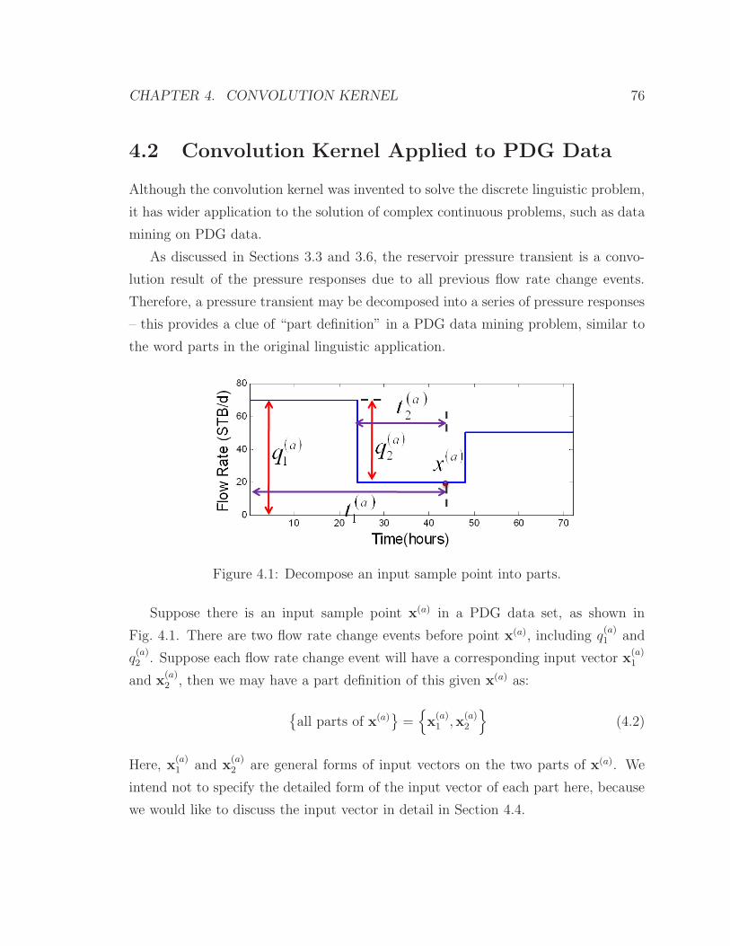
CHAPTER 4. CONVOLUTION KERNEL 76
4.2 Convolution Kernel Applied to PDG Data
Although the convolution kernel was invented to solve the discrete linguistic problem,
it has wider application to the solution of complex continuous problems, such as data
mining on PDG data.
As discussed in Sections 3.3 and 3.6, the reservoir pressure transient is a convo-
lution result of the pressure responses due to all previous flow rate change events.
Therefore, a pressure transient may be decomposed into a series of pressure responses
– this provides a clue of “part definition” in a PDG data mining problem, similar to
the word parts in the original linguistic application.
Figure 4.1: Decompose an input sample point into parts.
Suppose there is an input sample point x(a) in a PDG data set, as shown in
Fig. 4.1. There are two flow rate change events before point x(a), including q(a)1 and
q(a)2 . Suppose each flow rate change event will have a corresponding input vector x
(a)1
and x(a)2 , then we may have a part definition of this given x(a) as:
all parts of x(a)
=
x(a)1 ,x
(a)2
(4.2)
Here, x(a)1 and x
(a)2 are general forms of input vectors on the two parts of x(a). We
intend not to specify the detailed form of the input vector of each part here, because
we would like to discuss the input vector in detail in Section 4.4.

CHAPTER 4. CONVOLUTION KERNEL 77
Generally, for any input sample x(i), we have the parts definition as Eq. 4.3.
all parts of x(i)
=
x(i)1 ,x
(i)2 , . . . ,x
(i)k , . . . ,x
(i)Ni
(4.3)
Here, x(i)k is the general form of input vector of kth part of x(i), and Ni is the total
number of flow rate change events before x(i). Because it is very hard to detect all
breakpoints accurately, a wise solution is treat all points before the current sample
point as breakpoints. In this way, no breakpoint detection is required while the
accuracy is still maintained. In this way, Ni = i, and Eq. 4.3 becomes:
all parts of x(i)
=
x(i)1 ,x
(i)2 , . . . ,x
(i)k , . . . ,x
(i)i
(4.4)
With the parts defined, the second element of a convolution kernel is the simple
kernel. Supposing that we have two parts x(i)k and x
(j)l from two sample point x(i) and
x(j), the simple kernel we are going to use is the linear kernel, as shown in Eq. 4.5.
k(
x(i)k ,x
(j)l
)
=(
x(i)k
)T
x(j)l (4.5)
Finally, linearly combining all simple kernels evaluated on all possible part pairs,
we form the convolution kernel, as shown in Eq. 4.6.
K(
x(i),x(j))
=
Ni∑
k=1
Nj∑
l=1
k(
x(i)k ,x
(j)l
)
where k(
x(i)k ,x
(j)l
)
=(
x(i)k
)T
x(j)l (4.6)
As every point before the sample point is treated as a breakpoint to avoid the
requirement of accurate breakpoint detection, we have Ni = i and Nj = j. So that
the convolution kernel function is:
K(
x(i),x(j))
=
i∑
k=1
j∑
l=1
k(
x(i)k ,x
(j)l
)
where k(
x(i)k ,x
(j)l
)
=(
x(i)k
)T
x(j)l (4.7)
Selecting the linear summation to form the convolution kernel originates mainly
from the characteristics of the reservoir pressure transient. As discussed previously,

CHAPTER 4. CONVOLUTION KERNEL 78
the subsurface pressure is the convolution result of the pressure responses due to
previous flow rate change events. Specifically, the way of the convolution is linear
summation of all pressure responses, namely, superposition. Because the superpo-
sition linearly adds up all pressure responses which are “parts” in our convolution
kernel, it is quite intuitive to linearly combine all the simple kernels that evaluate
over the parts. This also helps us to implement the idea discussed in Section 3.6 that
a better deployment of the kernel functions would be superposition over kerneliza-
tion, rather than kernelization over the superposition. Linearly combining all simple
kernels exactly reflects the methodology of “superposition over kernelization”.
In addition to the response to the superposition, the linear summation also takes
advantage of the summation closure rules as discussed in Section 4.1, so that the
newly formed convolution kernel in Eq. 4.7 satisfies the requirement of a valid kernel
function.
In this way, a convolution kernel was successfully constructed for the data mining
of PDG data.
4.3 New Formulation for Conjugate Gradient
Before further moving on to the selection of the input vector, we would like to improve
the optimization method first. In the optimization method discussed in this section,
technical concepts including Conjugate Gradient and Reproducing Kernel Hilbert
Space were utilized. Actually, either topic of the two would form a book easily. It
was not the target of this study nor of this dissertation to explore the detailed theories
of the two topics. Therefore, only the useful conclusions related to the data mining
project are shown in this section. Deeper proof, derivation and theorems can be
obtained from the references.
In the simple study described in Chapter 3, the Steepest Gradient Descent (SGD)
method was used in the iterative training process. However, the SGD method is very
inefficient for two major reasons. For one reason, the SGD method has no limit on
the count of iterations before convergence. SGD may require a long time to finally
converge to the predefined residual, leading to a low efficiency of learning. For the

CHAPTER 4. CONVOLUTION KERNEL 79
other, the SGD method may follow zig-zag iterations when the Hessian matrix has
a large condition number (Caers, 2009). Therefore, it is necessary to improve the
optimization method to raise the overall efficiency of the data mining process.
The Conjugate Gradient (CG) method can usefully replace the SGD method. The
CG method may avoid the two disadvantages of SGD discussed earlier. For any linear
equation Ax = b, where A ∈ ℜn×n, and x,b ∈ ℜn, the CG method is searching in
a Krylov space generated by A and b, and the solution is going to converge in at
most n iterations (Trefethen and Bau, 1997). So there is no longer any zig-zag steps.
Fig 4.2 shows a comparison between CG and SGD methods solving a linear system
with n = 2. The CG method (red line) takes at most two steps to converge, while
SGD method (green line) zig-zags when approaching the optimum.
Figure 4.2: A comparison of the SGD method (in green) and CG method (in red) forminimizing a quadratic function associated with a given linear system. CG methodconverges in at most n steps (here n=2), while SGD method zig-zags when approach-ing the optimum, from Alexandrov (2007).
However, in order to utilize the CG method, we have to formulate a linear equation
such as Ax = b. In this case, we need to reformulate the training equation (Eq. 3.20)
and the prediction equation (Eq. 3.22) to adapt the CG method.

CHAPTER 4. CONVOLUTION KERNEL 80
In fact, each valid kernel function K (x, z) is positive-definite2, and associated
with a corresponding space of functions, HK, named reproducing kernel Hilbert space
(RKHS) (Hastie et al., 2009). The definitions of a Hilbert space and a reproducing
kernel Hilbert space are as follows.
Hilbert Space. A Hilbert space is an inner product space that is complete and sep-
arable with respect to the norm defined by the inner product. For example, the vector
space ℜn with the inner production definition as 〈x, z〉 = xTz.
Reproducing Kernel Hilbert Space (RKHS) (Evgeniou et al., 2000). A re-
producing kernel Hilbert space (RKHS) is a Hilbert space H of functions defined over
some bounded domain X ⊂ ℜn with the property that, for each x ∈ X, the evaluation
functionals defined as:
Fx[f] = f (x) ∀f ∈ H (4.8)
are linear, bounded functionals. The boundedness means that there exists a U = Ux∈
ℜ+ such that:
|Fx[f]| = |f (x)| ≤ U ‖f‖ (4.9)
for all f in the RKHS.
The relation between RKHS and Hilbert space is that a RKHS is a Hilbert
space where the inner product is defined using a positive-definite kernel function
K (x, z) (Evgeniou et al., 2000).
As mentioned at the beginning of the section, the RKHS is a profound topic,
about which it is not necessary to make further derivation or discussion. This section
will emphasize some items that are helpful to the PDG data mining task project:
1. Each positive-definite kernel function K (x, z) is associated with a RKHS HK,
while each RKHS HK corresponds to a unique positive-definite kernel function
K (x, z), named the reproducing kernel of HK (hence the terminology RKHS)
(Hastie et al., 2009; Evgeniou et al., 2000).
2To be exact, a valid kernel is positive semidefinite according to the Mercer Theorem (refer toSection 3.2 and Appendix B). However, the zero kernel is not useful. Here, in the dissertation, avalid kernel usually means a positive-definite kernel.

CHAPTER 4. CONVOLUTION KERNEL 81
2. Using a positive-definite kernel K (x, z) to do the machine learning is equiva-
lently finding a function f in the RKHS HK corresponding to K (x, z) such that
f (x) = y, where x ∈ ℜn is the general form of input vector, and y ∈ ℜ is the
general form of the observation (in the training process) or the prediction (in
the prediction process). n is the dimension of the input vector x, specifically,
in the context of this project n = Nx.
3. When the true function f in HK is not visible, but a data set (training data set)
is provided as(
x(i), y(i))
|x(i) ∈ ℜn, y(i) ∈ ℜ, i = 1, . . . , m
, the true function f
may be approached by the set of half evaluated functions K(
·,x(i))
. This could
be expressed mathematically (Wahba, 1990; Hastie et al., 2009) as:
fβ (x) =
m∑
i=1
βiK(
x,x(i))
(4.10)
Here, m is the total number of training data, specifically in the context of this
project, m = Np. The half evaluated function K(
·,x(i))
works as the basis func-
tion, which is also known as the representer of evaluation at x(i) (Hastie et al.,
2009), mathematically Kx(i) (x) = K
(
x,x(i))
(treat the x(i) as a parameter, and
x as the unknown variable). In this dissertation, we would like to name these
half evaluated kernel functions as kernel basis functions for simplicity.
These discussions of the kernel function and RKHS give us at least two impor-
tant hints regarding the kernelized learning. First, because the half evaluated kernel
function, K(
·,x(i))
, works as the basis function of HK to span the true function f,
the more training data(
x(i), y(i))
are provided, the more possible
K(
·,x(i))
will
form a complete basis, and the closer the function fβ will approach the true func-
tion f. This explains why the kernelized learning method (generally all data mining
methods) requires a large amount of data.
Secondly, we may summarize the ultimate target of the kernelized learning from a
new point of view, that is, the task of the kernelized learning is to find the coefficients
β such that function fβ (x) defined in Eq. 4.10 is an adequate estimator of the true
function f (Blanchard and Kramer, 2010).

CHAPTER 4. CONVOLUTION KERNEL 82
To obtain the coefficient β, the training data will be utilized. Substitute x =
x(1), y = y(1), then we have:
fβ(
x(1))
=
m∑
i=1
βiK(
x(1),x(i))
= y(1) (4.11)
Similarly for all training data, we have:
fβ(
x(1))
=∑m
i=1 βiK(
x(1),x(i))
= y(1)
...
fβ(
x(k))
=∑m
i=1 βiK(
x(k),x(i))
= y(k)
...
fβ(
x(m))
=∑m
i=1 βiK(
x(m),x(i))
= y(m)
(4.12)
Recall the definition of kernel matrix mentioned in the Mercer Theorem (refer to
Section 3.2), we define the kernel matrix as follows.
Kernel Matrix. Suppose a data set(
x(i), y(i))
|x(i) ∈ ℜn, y(i) ∈ ℜ, i = 1, . . . , m
is
given, and a valid kernel function K (x, z) is provided, a kernel matrix K may be
defined as
K =
K11 . . . K1j . . . K1m
......
...
Ki1 . . . Kij . . . Kim
......
...
Km1 . . . Kmj . . . Kmm
(4.13)
where:
Kij = K(
x(i),x(j))
(4.14)
Using the kernel matrix K, Equation 4.12 could be rewritten in the matrix form
as:
Kβ = y (4.15)

CHAPTER 4. CONVOLUTION KERNEL 83
where:
y =(
y(1), . . . , y(m))T
(4.16)
β = (β1, . . . , βm)T (4.17)
Applying Eq. 4.15 to the PDG data mining project, in which m = Np, the training
equation becomes:
Kβ = y (4.18)
where:
K =
Kij |Kij = K(
x(i),x(j))
, i, j = 1, . . . , Np
(4.19)
β =(
β1, . . . , βNp
)T(4.20)
y =(
yobs(1), . . . , yobs(Np))T
(4.21)
With β obtained by the matrix form training equation, Eq. 4.18, the prediction
equation is:
ypred =
Np∑
i=1
βiK(
xpred,x(i))
(4.22)
Eq. 4.18 and Eq. 4.22 are the new matrix form training and prediction equation
for the kernelized learning from now on. Furthermore, considering the new form of
training equation, Eq. 4.18, has a linear form, the CG method may be applied to
the learning process. Algorithm 3 shows the algorithm of applying the conjugate
gradient method on the training equation, Eq. 4.18, to obtain the coefficients β.
In the algorithm, the iteration loop is executed at most for Np times because the
conjugate gradient method converges in at most Np steps as long as the kernel matrix
is well-posed. However, because the CG method has a very good convergence rate, it
usually converge very quickly and does not need that many steps to converge.
As described to now, the learning method with convolution kernel successfully

CHAPTER 4. CONVOLUTION KERNEL 84
Algorithm 3 Learning with Conjugate Gradient Method
β[0] = ~0, r[0] = y, q[0] = r[0] initializationfor k = 1, 2, . . . , Np do
a[k] =r[k−1]Tr[k−1]
q[k−1]TKq[n−1]calculate step length
β[k] = β[k−1] + a[k]q[k−1] update solutionr[k] = r[k−1] − a[k]Kq[k−1] update residualif β[k] is convergent thenreturn β[k]
end if
b[k] =r[k]
Tr[k]
r[k−1]Tr[k−1]
q[k] = r[k] + b[k]q[k−1]update search directionend forreturn β[Np]
adapts the CG method as the optimization method. The last thing before the appli-
cation is to select a proper input vector for the parts in the convolution kernel.
4.4 Input Vector Selection
For the convolution kernel, an input vector still needs to be selected for the training
and prediction purposes. However, the input vector for the convolution kernel has
a slight difference to that of a simple kernel. For a simple kernel, one input vector
corresponds to one sampling point, while for the convolution kernel, one input vector
corresponds to one part of one sampling point. Mathematically, for each sampling
point(
t(i), q(i), p(i))
, there is only one corresponding input vector for the simple kernel
method such that:(
t(i), q(i), p(i))
→ x(i), (4.23)
However, there are a series of input vectors corresponding to all “parts” for this
sampling point, such that:
(
t(i), q(i), p(i))
→
x(i)k , k = 1, . . . , i
(4.24)

CHAPTER 4. CONVOLUTION KERNEL 85
The selection of the input vector for the convolution kernel is hence the selection of
x(i)k .
Table 3.2 in Section 3.3 shows a guidance for selection of the input vector corre-
sponding to some reservoir behaviors. Here, three choices are prepared as shown in
Table 4.1.
Table 4.1: Input vector for convolution kernel
KV3F KV4FA KV4FB
x(i)k =
q(i)k
q(i)k log t
(i)k
q(i)k t
(i)k
x(i)k =
q(i)k
q(i)k log t
(i)k
q(i)k t
(i)k
q(i)k
(
t(i)k
)2
x(i)k =
q(i)k
q(i)k log t
(i)k
q(i)k t
(i)k
q(i)k /t
(i)k
Inside, k = 1, . . . , i. The name for the first choice of the input vector, “KV3F”,
is the abbreviation for “kernel input vector with three features”. “KV4FA” and
“KV4FB” are two kinds of input vectors with four features.
In the input vector of KV4FB, q(i)k /t
(i)k is also added as the last feature. The
feature is added to capture those reservoir behaviors that decay with the elapsed
time, such as wellbore effect. Moreover, the exponential integral function Ei (x) =
−∫ +∞
−x
exp (−u)
udu is the main function in the solution of the synthetic constant
infinite-acting radial flow (Ramey, 1970; Horne, 1995), and q(i)k /t
(i)k is the main func-
tion of the second order approximation for the exponential integral function, so it is
important to improve accuracy of the prediction.
To test which kernel function results in the best prediction, three tests cases were
used as listed in Table 4.2. These test cases are the same as those in Table 3.5 in
Section 3.5, so the test case numbers are kept the same to maintain a consistency
throughout the whole dissertation.
Fig. 4.3 shows the result of three input vector (with convolution kernel) applied
on three test cases. Fig. 4.3(a) and Fig. 4.3(b) are the prediction results according
to a variable flow rate and a constant flow rate using three different input vectors
on Test Case 4. All three input vectors return good prediction in the variable flow

CHAPTER 4. CONVOLUTION KERNEL 86
Table 4.2: Test cases for convolution kernel input vector selection
Test Case # Test Case Characteristics
4 Infinite-acting radial flow + wellbore effect + skin7 Infinite-acting radial flow + wellbore effect + skin + closed
boundary8 Infinite-acting radial flow + wellbore effect + skin + constant
pressure boundary
rate case (Fig. 4.3(a)). However, in the constant flow rate case (Fig. 4.3(b)), KV3F
and KV4FA miss the wellbore storage at the beginning while KV4FB captures the
wellbore storage very well. After the short wellbore effect, all three methods capture
the infinity-acting radial flow with good accuracy.
Fig. 4.3(c) and Fig. 4.3(d) show the results on Test Case 7. In the log-log plot
(Fig. 4.3(d)) KV4FB clearly shows its advantage in capturing the wellbore storage,
but it has slight deviation on the infinite-acting radial flow. However, KV4FA misses
the wellbore storage but has an accurate prediction of the infinite-acting radial flow.
KV3F has deviation in both the wellbore storage and the infinite-acting radial flow
stages. All three input vectors have good prediction of the boundary behavior.
Fig. 4.3(e) and Fig. 4.3(f) are the results on Test Case 8. All three input vectors
work well in both the variable flow rate case and the constant flow rate case. KV4FB
has a best prediction in the log-log plot (Fig. 4.3(f)).
To sum up, all three input vectors have good prediction in all three test cases.
Comparably, KV3F and KV4FA miss the wellbore effect in Test Cases 4 and 7, while
KV4FB captures all the reservoir features well in all test cases except the small
deviation on the radial flow in Case 7. Finally, KV4FB was selected as the most
suitable input vector for the convolution kernel.

CHAPTER 4. CONVOLUTION KERNEL 87
0 20 40 60 80 100 120 140 160 180 200−900
−800
−700
−600
−500
−400
−300
−200
−100
0
Time (hours)
∆Pre
ssur
e (p
si)
True DataKV3FKV4FAKV4FB
(a) Case 4: Variable flow rate
100
101
102
102.1
102.3
102.5
102.7
102.9
Time (hours)
∆Pre
ssur
e (p
si)
True DataTrue Data (Derivative)KV3FKV3F (Derivative)KV4FAKV4FA (Derivative)KV4FBKV4FB (Derivative)
(b) Case 4: Constant Flow rate
0 20 40 60 80 100 120 140 160 180 200−1100
−1000
−900
−800
−700
−600
−500
−400
−300
−200
−100
Time (hours)
∆Pre
ssur
e (p
si)
True DataKV3FKV4FAKV4FB
(c) Case 7: Variable Flow rate
100
101
102
101
102
103
Time (hours)
∆Pre
ssur
e (p
si)
True DataTrue Data (Derivative)KV3FKV3F (Derivative)KV4FAKV4FA (Derivative)KV4FBKV4FB (Derivative)
(d) Case 7: Constant flow rate
0 20 40 60 80 100 120 140 160 180 200−900
−800
−700
−600
−500
−400
−300
−200
−100
0
Time (hours)
∆Pre
ssur
e (p
si)
True DataKV3FKV4FAKV4FB
(e) Case 8: Variable flow rate
100
101
102
101
102
103
Time (hours)
∆Pre
ssur
e (p
si)
True DataTrue Data (Derivative)KV3FKV3F (Derivative)KV4FAKV4FA (Derivative)KV4FBKV4FB (Derivative)
(f) Case 8: Constant flow rate
Figure 4.3: (a) and (b) show the results of variable flow rate and constant flow rateusing three different input vectors on Test Case 4. (c) and (d) show the results onTest Case 7. (e) and (f) show the results on Test Case 8. From the comparison in allthree test cases, KV4FB gives better prediction, especially in the detail of wellboreeffect.

CHAPTER 4. CONVOLUTION KERNEL 88
In addition, the input vector “KV5F” as shown in Eq. 4.25:
x(i)k =
q(i)k
q(i)k log t
(i)k
q(i)k t
(i)k
q(i)k
(
t(i)k
)2
q(i)k /t
(i)k
(4.25)
has also been investigated. In the study, we found that KV5F performed very close
to KV4FB in most of test cases, except some of the real data cases. In those real
cases, KV5F was sensitive and unstable, and made biased predictions. Therefore,
KV5F was finally rejected from the input vector candidates. We still would like to
document it here, as it might be reselected an input vector candidate someday after
future study regarding its characteristics. In addition, although KV3F and KV4FA
were not finally selected as the input vector, they are still very promising for the
convolution kernel method. In our study, they passed all test cases with reasonable
predictions. Especially KV3F has surprisingly good stability in very noisy cases
(with high percentage of outliers and aberrant segments). For further study and real
practice, KV3F and KV4FA are still worth further study and investigation.
Having selected the input vector, it is time to formally form a new method, Method
D, as the method using the convolution kernel. Table 4.3 shows the input vector and
kernel function for Method D. The next section describes the application of Method
D to a series of test cases.
4.5 Application
A series of test cases, listed in Table 4.4 were constructed to test the performance of
the convolution kernel method in different scenarios. Test Cases 1 through 9 are the
same as those discussed in Chapter 3. The test results are shown and discussed in
this section.
The test workflow for Test Cases 1-13 was formed as follows.

CHAPTER 4. CONVOLUTION KERNEL 89
Table 4.3: Input vector and kernel function for Method D
Method D
Input Vector x(i)k =
q(i)k
q(i)k log t
(i)k
q(i)k t
(i)k
q(i)k /t
(i)k
Kernel FunctionK(
x(i),x(j))
=∑i
k=1
∑j
l=1 k(
x(i)k ,x
(j)l
)
k(
x(i)k ,x
(j)l
)
=(
x(i)k
)T
x(j)l
1. Construct a synthetic pressure, flow rate data set, add 3% artificial noise (nor-
mally distributed) to both the pressure and the flow rate data.
2. Use the synthetic data set (with artificial noise) as the training data set. Apply
the convolution kernelized data mining algorithms (Method D) to learn the data
set until convergence.
3. Feed the data mining algorithm with the training variable flow rate history
(without noise) and collect the prediction from the data mining algorithm.
4. Compare the predicted pressure data (from Step 3) with the synthetic pressure
data without noise (from Step 1).
5. Feed the data mining algorithm with a constant flow rate history (without noise)
and collect the predicted pressures from the data mining algorithm.
6. Construct a synthetic pressure according to the constant flow rate in Step 5
using the same wellbore/reservoir model as Step 1.
7. Compare the predicted pressure data (from Step 5) with the synthetic pressure
data (from Step 6).
8. Feed the data mining algorithm with a multivariable flow rate history (without
noise) and collect the predicted pressures from the data mining algorithm.

CHAPTER 4. CONVOLUTION KERNEL 90
Table 4.4: Test cases for convolution kernel methodTest Case # Test Case Characteristics
1 Infinite-acting radial flow2 Infinite-acting radial flow + wellbore effect3 Infinite-acting radial flow + skin4 Infinite-acting radial flow + wellbore effect + skin5 Infinite-acting radial flow + closed boundary (pseudosteady
state)6 Infinite-acting radial flow + constant pressure boundary7 Infinite-acting radial flow + wellbore effect + skin + closed
boundary8 Infinite-acting radial flow + wellbore effect + skin + constant
pressure boundary9 Infinite-acting radial flow + dual porosity10 Infinite-acting radial flow + wellbore effect + skin + constant
pressure boundary + step flow rate history (Complicated Syn-thetic Case A)
11 Infinite-acting radial flow + wellbore effect + skin + constantpressure boundary + fast shifted flow rate history (Compli-cated Synthetic Case B)
12 Infinite-acting radial flow + wellbore effect + skin + constantpressure boundary + real flow rate history (Semireal Case A)
13 Infinite-acting radial flow + wellbore effect + skin + constantpressure boundary + real flow rate history (Semireal Case B)
14 real pressure + real flow rate history (Real Case A)15 real pressure + real flow rate history (Real Case B)37 real pressure + real flow rate history + cross validation (Real
Case C)

CHAPTER 4. CONVOLUTION KERNEL 91
9. Construct a synthetic pressure according to the multivariable flow rate in Step
9 using the same wellbore/reservoir model from Step 1.
10. Compare the predicted pressure data (from Step 8) with the synthetic pressure
data (from Step 9).
For the real case tests, Test Cases 14-15, and 37, there were no “true data” for
comparison, so the test workflow becomes:
1. Use the real data set as the training data set. Apply the convolution kernelized
data mining algorithms (Method D) to learn the data set until convergence.
2. Feed the data mining algorithm with the training variable flow rate history (real
flow rate history) and collect the prediction from the data mining algorithm.
3. Compare the predicted pressure data (from Step 2) with the real pressure data
(from Step 1).
4. Feed the data mining algorithm with a constant flow rate history (without noise)
and collect the predicted pressures from the data mining algorithm.
5. Feed the data mining algorithm with a multivariable flow rate history (without
noise) and collect the predicted pressures from the data mining algorithm.
The tests were conducted step by step, from synthetic to real cases. Test Cases 1-9
are synthetic test cases to test the convolution kernel working in different scenarios.
These nine tests are the same as those nine test cases for simple kernel methods,
listed in Table 3.5, aiming to compare the convolution kernel methods with the simple
kernel method. Therefore, both the predictions using Method D (convolution kernel
method) and Method B (simple kernel method) are displayed in the result plots. Test
Cases 10-11 are complicated synthetic cases, in which the flow rate history is changing
rapidly to represent the complex real reservoir production environment. Test Cases
12-13 are “semireal” field cases in which the training flow rate history is real while
the training pressure data were generated using the models. These two cases have
important meaning to us, because they are the closest artificial cases to the real field

CHAPTER 4. CONVOLUTION KERNEL 92
cases while we still have the true data for the comparison of prediction accuracy. Test
Cases 14-15 are real cases in which both the pressure and the flow rate data are real.
However, because there are no “true data” for the real cases, there is no known true
answer for comparison. Test Case 37 is another real case with nearly nine months
of production data. In this case, a cross validation was performed, in which the real
data set was divided into two parts that were used for training data set and test data
set respectively. The target of this case was to validate the prediction result using
the real data set itself.
The same test cases have the same test case number throughout the whole disser-
tation, such as Test Cases 1-9 in the tests for both simple kernel method in Section 3.5
and convolution kernel method in this chapter. Case 37 was added later than other
cases in the following chapters, so the case number is not adjacent. The model data
for all test cases are listed in Appendix A.
The test results are shown in four kinds of plots, including:
• a Cartesian plot of the training data (noisy data) and the true data (no noise
data). For the real data cases, no true data will be plotted.
• a Cartesian plot of the prediction to the variable flow rate history (training data
set reproduction)
• a log-log plot of the prediction to the constant flow rate history
• a Cartesian plot of the prediction to the multivariable flow rate history (more
variable flow rate prediction)
For simplicity, not all the plots are shown for all test cases as not all are relevant.
Table 4.5 shows which plots are shown for each test case. The test cases and their
results are discussed one by one in the following 16 subsections.
4.5.1 Case 1: Infinite-acting Radial Flow
The same as in Section 3.5.1, Case 1 is the simplest case with only one reservoir
behavior, infinite-acting radial flow. Fig. 4.4(a) shows the training data set (pink

CHAPTER 4. CONVOLUTION KERNEL 93
Table 4.5: Result plots for all tests on convolution kernel method
Test Case # Training/TrueData
Variable FlowRate
ConstantFlow Rate
Multi-Variable Flow
Rate
1 X X X2 X X3 X X4 X X X5 X X6 X X7 X X X8 X X X9 X X10 X X X X11 X X X X12 X X X X13 X X X X14 X X X X15 X X X X37 X X X (cross
validation)

CHAPTER 4. CONVOLUTION KERNEL 94
line) and the true data (blue line). Both the flow rate and the pressure data had
added 3% artificial noise (normally distributed). Although the true data are shown
in the figures, they are not visible to the data mining process. In the test, only the
noisy data were provided to the machine learning algorithms. The true data are
shown here for comparison purpose only. For Tests 2-9, the figures for the training
data are omitted for simplicity.
In the variable flow rate prediction (Fig. 4.4(b)), Method B and Method both
give very good prediction compared with the true data. In the constant flow rate
prediction (Fig. 4.4(c)), the log-log plot shows that Methods B and D both capture
the overall infinite-acting radial flow behavior. However, Method B has a drop in the
derivative curve in the last half log cycle, while Method D has no such problem. The
half log cycle problem for Method B has been discussed in Section 3.6. At that time,
we anticipated a new architecture of kernel function and superposition might retrieve
better results. Here, the convolution kernel method (Method D) shows its advantage
to the simple kernel method at least in this specific kind of example.
4.5.2 Case 2: Infinite-acting Radial Flow + Wellbore Effect
Fig. 4.5 demonstrates the results of Method D working on an infinite-acting radial
flow with wellbore storage effect. Method B still shows a drop-off in the last half
log cycle in the derivative curve in Fig. 4.5(b), while Method D captures the infinite-
acting radial flow as well as the wellbore storage effect. In Fig. 4.5(a), the two methods
make very good reproduction of pressure transients according to the variable flow rate
history. As discussed in Section 3.5, the sampling of the data leads to the absence
of the early time data (data in the range [10−3h, 1h]), so the unit straight line of the
wellbore storage effect in the derivative curve is not seen in the figure. However, the
appearance of the pressure prediction showing the end of the hump of the pressure
derivative could be treated as an indirect demonstration that Method D still captures
the wellbore effect.

CHAPTER 4. CONVOLUTION KERNEL 95
0 50 100 150 200−1000
−500
0
Time (hours)
∆Pre
ssur
e (p
si)
True DataNoisy Data
0 50 100 150 200
0
20
40
60
80
Time (hours)Flo
w R
ate
(ST
B/d
)
True DataNoisy Data
(a)
0 20 40 60 80 100 120 140 160 180 200−800
−700
−600
−500
−400
−300
−200
−100
0
Time (hours)
∆Pre
ssur
e (p
si)
True DataMethod BMethod D
(b)
100
101
102
101
102
103
Time (hours)
∆Pre
ssur
e (p
si)
True DataTrue Data (Derivative)Method BMethod B (Derivative)Method DMethod D (Derivative)
(c)
Figure 4.4: Data mining results using convolution kernel method on Case 1: (a) thetraining data set; (b) prediction using the variable flow rate history; (c) predictionusing the constant flow rate history on a log-log plot.

CHAPTER 4. CONVOLUTION KERNEL 96
0 20 40 60 80 100 120 140 160 180 200−800
−700
−600
−500
−400
−300
−200
−100
0
Time (hours)
∆Pre
ssur
e (p
si)
True DataMethod BMethod D
(a)
100
101
102
102.1
102.2
102.3
102.4
102.5
102.6
102.7
102.8
Time (hours)
∆Pre
ssur
e (p
si)
True DataTrue Data (Derivative)Method BMethod B (Derivative)Method DMethod D (Derivative)
(b)
Figure 4.5: Data mining results using convolution kernel method on Case 2: (a)prediction using the variable flow rate history; (b) prediction using the constant flowrate history on a log-log plot.
4.5.3 Case 3: Infinite-acting Radial Flow + Skin
Case 3 is a synthetic case with infinite-acting radial flow and a skin effect. The
results are shown in Fig. 4.6. The true pressure in this case has similar shape to
that in Case 1, as shown in Fig. 4.6(b) and Fig. 4.4(c). However, the factor of the
skin did affect the prediction of Method B, leading to a hump in the early stage of
infinite-acting radial flow and a drop at the last log cycle in Fig. 4.4(c). However,
Method D using the convolution kernel still makes the prediction with high precision.
In the Cartesian plot (Fig. 4.6(a)), at the corner near 120 hours, Method B deviates
slightly from the true data while Method D makes a sharp corner prediction that is
a better representation of the true data.
4.5.4 Case 4: Infinite-acting Radial Flow + Wellbore Effect
+ Skin
Fig. 4.7 shows the results applying the simple kernel method (Method B) and con-
volution kernel method (Method D) on Case 4 which includes infinite-acting radial
flow, wellbore effect and skin factor. Fig. 4.7(a) shows the pressure reproduction of
the variable flow rate history, in which the two methods both give good prediction.

CHAPTER 4. CONVOLUTION KERNEL 97
0 20 40 60 80 100 120 140 160 180 200−900
−800
−700
−600
−500
−400
−300
−200
−100
0
Time (hours)
∆Pre
ssur
e (p
si)
True DataMethod BMethod D
(a)
100
101
102
101
102
103
Time (hours)
∆Pre
ssur
e (p
si)
True DataTrue Data (Derivative)Method BMethod B (Derivative)Method DMethod D (Derivative)
(b)
Figure 4.6: Data mining results usign convolution kernel method on Case 3: (a)prediction using the variable flow rate history; (b) prediction using the constant flowrate history on a log-log plot.
In the constant flow rate prediction (Fig. 4.7(b)), Method B has a drop in the last
half log cycle, while Method D maintains good prediction until the end. In this case,
the multivariable flow rate prediction results are also shown in Fig. 4.7(c). The figure
clearly shows the advantage of Method D compared to the big deviation of Method
B. In Section 3.6, we have discussed that failing to predict multivariable flow rate
history greatly limits the application of Method B. Here, Fig. 4.7(c) demonstrates
that Method D overcomes this limitation successfully.
4.5.5 Case 5: Infinite-acting Radial Flow + Closed Boundary
(Pseudosteady State)
Sections 4.5.5 to 4.5.8 show the tests on Cases 5-8 that have boundary effect. Fig. 4.8
shows the results for Case 5 containing infinite-acting radial flow together with a
closed boundary (pseudosteady state). The two methods made good prediction to the
variable flow rate history, as shown in Fig. 4.8(a). However, in the pressure prediction
to the constant flow rate (Fig. 4.8(b)), both Method B and Method D deviated slightly
from the true infinite-acting radial flow region. Comparably, Method B is closer to
the true answer. Both methods captured the pseudosteady state boundary.

CHAPTER 4. CONVOLUTION KERNEL 98
0 20 40 60 80 100 120 140 160 180 200−900
−800
−700
−600
−500
−400
−300
−200
−100
0
Time (hours)
∆Pre
ssur
e (p
si)
True DataMethod BMethod D
(a)
100
101
102
102.1
102.3
102.5
102.7
102.9
Time (hours)∆P
ress
ure
(psi
)
True DataTrue Data (Derivative)Method BMethod B (Derivative)Method DMethod D (Derivative)
(b)
0 20 40 60 80 100 120 140 160 180 200
−800
−700
−600
−500
−400
−300
−200
−100
0
Time (hours)
∆Pre
ssur
e (p
si)
True DataMethod BMethod D
(c)
Figure 4.7: Data mining results usign convolution kernel methods on Case 4: (a)prediction using the variable flow rate history; (b) prediction using the constant flowrate history on a log-log plot; (c) prediction using the multivariable flow rate historyon a Cartesian plot.

CHAPTER 4. CONVOLUTION KERNEL 99
0 20 40 60 80 100 120 140 160 180 200−1000
−900
−800
−700
−600
−500
−400
−300
−200
−100
Time (hours)
∆Pre
ssur
e (p
si)
True DataMethod BMethod D
(a)
100
101
102
101
102
103
Time (hours)
∆Pre
ssur
e (p
si)
True DataTrue Data (Derivative)Method BMethod B (Derivative)Method DMethod D (Derivative)
(b)
Figure 4.8: Data mining results using convolution kernel method on Case 5: (a)prediction using the variable flow rate history; (b) prediction using the constant flowrate history on a log-log plot.
4.5.6 Case 6: Infinite-acting Radial Flow + Constant Pres-
sure Boundary
Case 6 studied the infinite-acting radial flow with constant pressure boundary. The
results are shown in Fig. 4.9. The two methods both had good pressure reproduction
of the variable flow rate, illustrated in Fig. 4.9(a). In the prediction to a constant flow
rate history, as shown in Fig. 4.9(b), Method B had a big drop at the constant pressure
boundary stage. Method D deviated slightly from the true data at the very end of
the constant pressure boundary, but overall followed the trend well. Comparably,
Method D was preferred in this case.
4.5.7 Case 7: Infinite-acting Radial Flow + Wellbore Effect
+ Skin + Closed Boundary
This case is a case with four kinds of reservoir behaviors together, including infinite-
acting radial flow, wellbore effect, skin factor and a closed boundary. Fig. 4.10 shows
the results of Method B and Method D. The two methods made good pressure repro-
duction to the variable flow rate history, as shown in Fig. 4.10(a). In Fig. 4.10(b),
Method B captured all reservoir features well, including in the early stage of wellbore

CHAPTER 4. CONVOLUTION KERNEL 100
0 20 40 60 80 100 120 140 160 180 200−800
−700
−600
−500
−400
−300
−200
−100
0
Time (hours)
∆Pre
ssur
e (p
si)
True DataMethod BMethod D
(a)
100
101
102
101
102
103
Time (hours)
∆Pre
ssur
e (p
si)
True DataTrue Data (Derivative)Method BMethod B (Derivative)Method DMethod D (Derivative)
(b)
Figure 4.9: Data mining results using convolution kernel method on Case 6: (a)prediction using the variable flow rate history; (b) prediction using the constant flowrate history on a log-log plot.
effect, the middle stage of radial flow, and the end stage of the pseudosteady state
boundary. Comparably, Method D captured the wellbore effect as well as the pseu-
dosteady state boundary but had slight deviation during the radial flow. However,
Method B did not maintain its good performance in the prediction to a multivariable
flow rate history, as shown in Fig. 4.10(c). Method B only predicted the overall trend
of the pressure, but lost the accuracy in the absolute value. Meanwhile, Method D
demonstrated its stability and accuracy in that it had good prediction to the mul-
tivariable flow rate history. Compared to the small deviation in Fig. 4.10(b), this
stability and accuracy in the multivariable flow rate prediction is preferable.
4.5.8 Case 8: Infinite-acting Radial Flow + Wellbore Effect
+ Skin + Constant Pressure Boundary
Case 8 is similar to Case 7 that contains four reservoir/well features except that Case 7
has a closed boundary while Case 8 has a constant pressure boundary. As in previous
cases, the two methods worked well in pressure reproduction to the variable flow rate,
as shown in Fig. 4.11(a). In Fig. 4.11(b), Method B and Method D both made good
pressure prediction to the constant flow rate, capturing correctly the wellbore effect,
skin, infinite-acting radial flow, and the boundary. In Fig. 4.11(c), as in the previous

CHAPTER 4. CONVOLUTION KERNEL 101
0 20 40 60 80 100 120 140 160 180 200−1100
−1000
−900
−800
−700
−600
−500
−400
−300
−200
−100
Time (hours)
∆Pre
ssur
e (p
si)
True DataMethod BMethod D
(a)
100
101
102
101
102
103
Time (hours)
∆Pre
ssur
e (p
si)
True DataTrue Data (Derivative)Method BMethod B (Derivative)Method DMethod D (Derivative)
(b)
0 20 40 60 80 100 120 140 160 180 200−900
−800
−700
−600
−500
−400
−300
−200
−100
0
Time (hours)
∆Pre
ssur
e (p
si)
True DataMethod BMethod D
(c)
Figure 4.10: Data mining results using convolution kernel method on Case 7: (a)prediction using the variable flow rate history; (b) prediction using the constant flowrate history on a log-log plot; (c) prediction using the multivariable flow rate historyon a Cartesian plot.

CHAPTER 4. CONVOLUTION KERNEL 102
case, Method B failed to predict to the multivariable flow rate history, while Method
D still made good prediction.
The prediction results to the multivariable flow rate histories in Cases 4, 7 and 8
demonstrate that Method D overcomes the limitation of Method B, so that Method D
maintains accurate prediction even to the multivariable flow rate history. Although
there were no prediction results shown to the multivariable flow rate histories in
Cases 1-3, and 5-6, actually the tests have also been carried out that Method D made
accurate prediction to the multivariable flow rate history in those cases as well.
0 20 40 60 80 100 120 140 160 180 200−900
−800
−700
−600
−500
−400
−300
−200
−100
0
Time (hours)
∆Pre
ssur
e (p
si)
True DataMethod BMethod D
(a)
100
101
102
101
102
103
Time (hours)
∆Pre
ssur
e (p
si)
True DataTrue Data (Derivative)Method BMethod B (Derivative)Method DMethod D (Derivative)
(b)
0 20 40 60 80 100 120 140 160 180 200
−700
−600
−500
−400
−300
−200
−100
0
Time (hours)
∆Pre
ssur
e (p
si)
True DataMethod BMethod D
(c)
Figure 4.11: Data mining results using convolution kernel method on Case 8: (a)prediction using the variable flow rate history; (b) prediction using the constant flowrate history on a log-log plot; (c) prediction using the multivariable flow rate historyon a Cartesian plot.

CHAPTER 4. CONVOLUTION KERNEL 103
4.5.9 Case 9: Infinite-acting Radial Flow + Dual Porosity
Fig. 4.12 demonstrates the prediction results in the dual porosity case. In Fig. 4.12(a),
Method D made better prediction around the corner near 120 hours, but overall,
the two methods’ predictions were acceptable. In the log-log plot of the pressure
prediction to the constant flow rate, the two methods deviated from the true answer,
but Method D captured the trend of the derivative curve. In addition, the final stage
of Method B’s prediction shows very strong instability that the derivative increased
and decreased abruptly. Method D performed much more stably, and even caught
the final stage of the derivative.
0 20 40 60 80 100 120 140 160 180 200−800
−700
−600
−500
−400
−300
−200
−100
0
100
Time (hours)
∆Pre
ssur
e (p
si)
True DataMethod BMethod D
(a)
100
101
102
10−2
10−1
100
101
102
103
Time (hours)
∆Pre
ssur
e (p
si)
True DataTrue Data (Derivative)Method BMethod B (Derivative)Method DMethod D (Derivative)
(b)
Figure 4.12: Data mining results using convolution kernel methods on Case 9: (a)prediction using the variable flow rate history; (b) prediction using the constant flowrate history on a log-log plot.
Until this case, all nine cases that have been carried out on the simple kernel
method in Section 3.5 were also tested using the convolution kernel method, Method
D. From the comparison between Method B and Method D, we may see that Method
D made stable and accurate prediction in different scenarios, no matter whether to
a variable flow rate, a constant flow rate or a multivariable flow rate. Method D
captured the early stage behavior such as wellbore effect as well as the late stage
behavior such as the boundary effect.
From next subsection, the tests of more complicated cases will be reported. In
these tests, only Method D was applied, and hence, only the Method D results are

CHAPTER 4. CONVOLUTION KERNEL 104
shown in the plots.
4.5.10 Case 10: Complicated Synthetic Case A
The study tried to evaluate the method step by step, from easy synthetic cases (Cases
1-9) to complicated synthetic cases (Cases 10 and 11), to semireal cases (Cases 12
and 13), and finally to real field cases (Cases 14-15 and 37). This section reports
the test results using Case 10, a complicated case that contains infinite-acting radial
flow, wellbore effect, skin factor, constant pressure boundary, and step-like flow rate
history.
Fig. 4.13(a) demonstrates the true data (blue line) and the noisy data (the pink
line). The true data were used for comparison purpose only and were not visible to the
data mining algorithm in the whole process. The noisy data were used as the training
data. In Fig. 4.13(a), we may see that the flow rate decreased and increased in a step
shape. Actually, in real field practice, the flow rate is often controlled in steps. We
therefor. constructed such a case to test whether the learning algorithm may function
well in the step-like flow rate change environment. Furthermore, the step-like flow
rate changes enhanced the pressure convolution, and shortened the constant flow rate
period such that the pressure transient had insufficient time to develop fully. All
these factors made the learning more difficult.
However, the pressure reproduction in Fig. 4.13(b) shows that the difficulty did
not affect the performance of Method D. The pressure reproduction is identical to the
true data. Fig. 4.13(c) and Fig. 4.13(d) show the prediction to a constant flow rate
history and a mutivariable flow rate history. The pressure predictions are accurate
in the two plots. Considering the fact that the true data was not known in advance
by the learning algorithm, and that what the learning algorithm knew was only the
noisy data, the pink line in Fig 4.13(a), it is clear that Method D did discover the
controlling logic of the reservoir behavior behind the noisy data set.

CHAPTER 4. CONVOLUTION KERNEL 105
0 50 100 150 200−1000
−500
0
Time (hours)
∆Pre
ssur
e (p
si)
True DataNoisy Data
0 50 100 150 200
0
20
40
60
80
Time (hours)Flo
w R
ate
(ST
B/d
)
True DataNoisy Data
(a)
0 20 40 60 80 100 120 140 160 180 200−900
−800
−700
−600
−500
−400
−300
−200
−100
0
Time (hours)
∆Pre
ssur
e (p
si)
True DataMethod D
(b)
100
101
102
101
102
103
Time (hours)
∆Pre
ssur
e (p
si)
True DataTrue Data (Derivative)Method DMethod D (Derivative)
(c)
0 20 40 60 80 100 120 140 160 180 200−800
−700
−600
−500
−400
−300
−200
−100
0
Time (hours)
∆Pre
ssur
e (p
si)
True DataMethod D
(d)
Figure 4.13: Data mining results using convolution kernel method on Case 10: (a) thetraining data set; (b) prediction using the variable flow rate history; (c) prediction us-ing the constant flow rate history on a log-log plot; (d) prediction using multivariableflow rate history on a Cartesian plot.

CHAPTER 4. CONVOLUTION KERNEL 106
4.5.11 Case 11: Complicated Synthetic Case B
Case 11 is reported in this section. Case 11 is a case that contains the infinite-
acting radial flow, wellbore effect, skin factor, constant pressure boundary, and a fast
shifting flow rate history. The true data and the noisy training data are shown in
Fig. 4.14(a). The figures show that the flow rate history changes every 10 hours,
leading to a wave-like pressure transient. These fast shifting flow rates contribute to
the pressure convolution very significantly. Also because of their short duration, each
single constant flow rate period was not sufficient to develop full reservoir behavior.
In the forward model, at least 30 hours was required for the pressure to respond
to the boundary, so in the training data set, no single piece of the constant flow
rate period and the corresponding pressure transient would reveal the overall model
of the well and the reservoir. The machine learning algorithm has to dig into the
convoluted pressure to obtain the well/reservoir model. In the test plan, it would
indicate a successful learning if the pressure prediction to a constant flow rate showed
a boundary in addition to the infinite-acting radial flow,
The learning and prediction results did not disappoint. Fig. 4.14(b) shows a very
good reproduction of the pressure response to the true flow rate history. At the same
time, Fig. 4.14(c) demonstrates the pressure prediction to a constant flow rate. The
plot shows that Method D captured the constant pressure boundary response from
the highly convoluted pressure transient, even thought no single period of constant
flow rate provided the overall description of the reservoir and the well. This shows the
merit of the data mining in the interpretation of PDG data in that the data mining
method may extract the reservoir and well model from a collection of pieces of data
even if each piece of data was not diagnostic by itself from a conventional well test
point of view. Fig. 4.14(d) shows the pressure prediction to a multivariable flow rate
history. The prediction is also very accurate compared to the true data.
The results of Cases 10 and 11 illustrated that Method D was capable of extracting
the well/reservoir model in the noisy and frequent changing environment. This is very
promising in that it reveals value in the PDG data that was previously ignored.

CHAPTER 4. CONVOLUTION KERNEL 107
0 50 100 150 200−1000
−800
−600
−400
−200
Time (hours)
∆Pre
ssur
e (p
si)
0 50 100 150 200
20
40
60
80
Time (hours)Flo
w R
ate
(ST
B/d
)
True DataNoisy Data
(a)
0 20 40 60 80 100 120 140 160 180 200
−900
−800
−700
−600
−500
−400
−300
Time (hours)∆P
ress
ure
(psi
)
True DataMethod D
(b)
100
101
102
101
102
103
Time (hours)
∆Pre
ssur
e (p
si)
True DataTrue Data (Derivative)Method DMethod D (Derivative)
(c)
0 20 40 60 80 100 120 140 160 180 200−800
−700
−600
−500
−400
−300
−200
−100
0
Time (hours)
∆Pre
ssur
e (p
si)
True DataMethod D
(d)
Figure 4.14: Data mining results using convolution kernel method on Case 11: (a) thetraining data set; (b) prediction using the variable flow rate history; (c) prediction us-ing the constant flow rate history on a log-log plot; (d) prediction using multivariableflow rate history on a Cartesian plot.

CHAPTER 4. CONVOLUTION KERNEL 108
4.5.12 Case 12: Semireal Case A
Sections 4.5.12 and 4.5.13 discuss two semireal cases, Case 12 and Case 13. In
the semireal cases, the flow rate data were from a real data set, while the pressure
data were generated using the forward model. The cases were designed to mimic the
real reservoir setting while maintaining the knowledge of the well/reservoir model.
This setting helps us to simulate the real field data but having the model available
for comparison purposes. The flow rate history of Case 12 selected a small piece of
production history, while that of Case 13 was longer.
Case 12 is a case in which infinite-acting radial flow, wellbore effect, skin factor,
and constant pressure boundary behavior all existed. Fig. 4.15(a) shows the true
data and the noisy data. Fig. 4.15(b) shows the pressure reproduction according
to the true flow rate history. In the training data, the real reservoir pressure data
were mixed with 3% artificial noise in the period of [120h, 130h]. However, in the
pressure prediction in Fig. 4.15(b) only the true reservoir pressure changes are seen,
and the noise is no longer apparent. This demonstrates that from the training process
the learning algorithm recognized what is real reservoir behavior and what is noise.
The advantage of the learning method specifically provides one of our study targets,
denoising. If using other denoising methods that generally smooth the curve, such
as Fast Fourier Transform (FFT) method, any small variation of the real reservoir
response would be included together with the noise. The real reservoir response which
might represent some specific reservoir events would then be lost. The denoising
provided by Method D works at a high resolution giving potentially more useful
information to the engineers.
Fig. 4.15(c) shows the pressure prediction to a constant flow rate. The learning
algorithm discovered all the preset well/reservoir features in the forward model. This
effectively achieves deconvolution. Fig. 4.15(d) demonstrates the pressure prediction
to a multivariable flow rate history. The pressure prediction is accurate compared to
the true data.

CHAPTER 4. CONVOLUTION KERNEL 109
0 50 100 150 200−600
−400
−200
0
Time (hours)
∆Pre
ssur
e (p
si)
True DataNoisy Data
0 50 100 150 200
0
20
40
Time (hours)Flo
w R
ate
(ST
B/d
)
True DataNoisy Data
(a)
0 20 40 60 80 100 120 140 160 180 200−500
−450
−400
−350
−300
−250
−200
−150
−100
−50
0
Time (hours)∆P
ress
ure
(psi
)
True DataMethod D
(b)
100
101
102
101
102
103
Time (hours)
∆Pre
ssur
e (p
si)
True DataTrue Data (Derivative)Method DMethod D (Derivative)
(c)
0 20 40 60 80 100 120 140 160 180 200−800
−700
−600
−500
−400
−300
−200
−100
0
Time (hours)
∆Pre
ssur
e (p
si)
True DataMethod D
(d)
Figure 4.15: Data mining results using convolution kernel method on Case 12: (a) thetraining data set; (b) prediction using the variable flow rate history; (c) prediction us-ing the constant flow rate history on a log-log plot; (d) prediction using multivariableflow rate history on a Cartesian plot.

CHAPTER 4. CONVOLUTION KERNEL 110
4.5.13 Case 13: Semireal Case B
Fig. 4.16 shows the test results on the second semireal case, Case 13. In Case 13,
the infinite-acting radial flow, wellbore effect, skin factor, and the constant pressure
boundary behavior all existed. The true data and the training data are shown in
Fig. 4.16(a). In this case, the flow rate history is longer and with more flow rate
changes than Case 12.
Fig. 4.16(b) shows the pressure reproduction to the true flow rate history. Similar
to Case 12, the data mining algorithm detected the real reservoir behavior from within
the noise, and made accurate pressure prediction. Fig. 4.16(c) shows the pressure
prediction to a constant flow rate history. Method D captured the infinite-acting
radial flow, skin factor, and the constant pressure boundary, but it deviated from the
true data in the wellbore effect stage. Fig. 4.16(d) shows a good pressure prediction
to the multivariable flow rate. Although Method D missed the wellbore effect in the
prediction to the constant flow rate, the overall prediction still proves its efficiency
and accuracy.
Including the two semireal cases, the convolution kernel method, Method D,
worked out all test scenarios.
4.5.14 Case 14: Real Case A
Sections 4.5.14 and 4.5.15 report the results of applying Method D on two real cases,
Case 14 and Case 15. Because they are real field cases, the reservoir model is not
known. Therefore, in the plots, only the prediction and the real data are shown.
Similarly, the artificial noise was not added to the training data, hence feeding the
machine learning algorithm with the original flavor of the real data set. Case 14 and
Case 15 were two sections of a real field data set, a short section and a long section
respectively, to illustrate the method working in different settings.
The results of Case 14 are shown in Fig. 4.17. The real data are shown in
Fig. 4.17(a). The pressure reproduction according to the real flow rate history is
shown in Fig. 4.17(b). The figure shows that Method D reproduced well the original
real data set, and honored many details of the real data.

CHAPTER 4. CONVOLUTION KERNEL 111
0 50 100 150 200−1500
−1000
−500
0
Time (hours)
∆Pre
ssur
e (p
si)
True DataNoisy Data
0 50 100 150 200
0
20
40
60
80
Time (hours)Flo
w R
ate
(ST
B/d
)
True DataNoisy Data
(a)
0 20 40 60 80 100 120 140 160 180 200−1200
−1000
−800
−600
−400
−200
0
Time (hours)
∆Pre
ssur
e (p
si)
True DataMethod D
(b)
100
101
102
101
102
103
Time (hours)
∆Pre
ssur
e (p
si)
True DataTrue Data (Derivative)Method DMethod D (Derivative)
(c)
0 20 40 60 80 100 120 140 160 180 200−800
−700
−600
−500
−400
−300
−200
−100
0
Time (hours)
∆Pre
ssur
e (p
si)
True DataMethod D
(d)
Figure 4.16: Data mining results using convolution kernel method on Case 13: (a) thetraining data set; (b) prediction using the variable flow rate history; (c) prediction us-ing the constant flow rate history on a log-log plot; (d) prediction using multivariableflow rate history on a Cartesian plot.

CHAPTER 4. CONVOLUTION KERNEL 112
Fig. 4.17(c) and Fig. 4.17(d) demonstrate the pressure prediction to a constant
flow rate and a multivariable flow rate. Fig. 4.17(c) suggests an infinite-acting ra-
dial flow region and a constant pressure boundary region in the derivative curve.
No wellbore storage effect was suggested. We would like to emphasize an impor-
tant use of the data mining pressure prediction. Supposing that the data mining
method successfully retrieved the well/reservoir properties, Fig. 4.17(c) reflects the
same well/reservoir pressure response according to a constant flow rate. Therefore,
the features obtained in Fig. 4.17(c) are the features of the well/reservoir. In other
words, the data mining method, Method D was reporting that the PDG well did
not have strong wellbore effect, but the producing reservoir had a constant pressure
boundary. Also the engineer could obtain the permeability and investigated radius
from the prediction in Fig. 4.17(c) using conventional well testing methods. All this
information regarding the well/reservoir model properties is actually extracted by the
data mining algorithms. Without the data mining algorithms, it would be very hard
for the engineer to identify that useful information from the raw PDG data shown in
Fig. 4.17(a). Here lays the great merit of the data mining methods.
4.5.15 Case 15: Real Case B
Case 15 is a second real field case with longer production period as shown in Fig. 4.18(a).
Fig. 4.18(b) demonstrates the pressure reproduction to the real flow rate history. In
Fig. 4.18(b) shows that Method D captured the overall trend and most of the details,
such as the sudden pressure peak and pressure variation in the curve corners. How-
ever, the pressure reproduction also reported a deviation of about 10 psi at the late
stage of the pressure curve. We actually do not know the meaning of this deviation,
either reflecting an inaccuracy brought by the data mining method, or implying some
unknown reservoir events that changed the nature of the pressure response over time.
For the sake of real practice, this prediction is indeed a good clue for some further
investigation regarding the reservoir production.
Actually, from the pressure prediction to a constant flow rate (Fig. 4.18(c)) and a
multivariable flow rate (Fig. 4.18(d)), we can have some confidence in the prediction.

CHAPTER 4. CONVOLUTION KERNEL 113
332 334 336 338 340 342 344 346 348 350 352−400
−300
−200
−100
0
Time (days)
∆Pre
ssur
e (p
si)
Real Data
332 334 336 338 340 342 344 346 348 350 3520
0.5
1
1.5
2
x 104
Time (days)Flo
w R
ate
(ST
B/d
)
Real Data
(a)
332 334 336 338 340 342 344 346 348 350 352−400
−350
−300
−250
−200
−150
−100
−50
Time (days)
∆Pre
ssur
e (p
si)
Real DataMethod D
(b)
100
101
102
103
10−1
100
101
102
Time (days)
∆Pre
ssur
e (p
si)
Method DMethod D (Derivative)
(c)
0 20 40 60 80 100 120 140 160 180 200−10
−9
−8
−7
−6
−5
−4
−3
−2
−1
0
Time (days)
∆Pre
ssur
e (p
si)
Method D
(d)
Figure 4.17: Data mining results using convolution kernel method on Case 14: (a) thetraining data set; (b) prediction using the variable flow rate history; (c) prediction us-ing the constant flow rate history on a log-log plot; (d) prediction using multivariableflow rate history on a Cartesian plot.

CHAPTER 4. CONVOLUTION KERNEL 114
200 300 400 500 600 700 800 900 1000−400
−300
−200
−100
0
Time (days)
∆Pre
ssur
e (p
si)
Real Data
200 300 400 500 600 700 800 900 10000
0.5
1
1.5
2
x 104
Time (days)Flo
w R
ate
(ST
B/d
)
Real Data
(a)
200 300 400 500 600 700 800 900 1000−400
−350
−300
−250
−200
−150
−100
−50
0
Time (days)∆P
ress
ure
(psi
)
Real DataMethod D
(b)
100
101
102
103
10−1
100
101
102
Time (days)
∆Pre
ssur
e (p
si)
Method DMethod D (Derivative)
(c)
0 20 40 60 80 100 120 140 160 180 200−12
−10
−8
−6
−4
−2
0
Time (days)
∆Pre
ssur
e (p
si)
Method D
(d)
Figure 4.18: Data mining results using convolution kernel method on Case 15: (a) thetraining data set; (b) prediction using the variable flow rate history; (c) prediction us-ing the constant flow rate history on a log-log plot; (d) prediction using multivariableflow rate history on a Cartesian plot.

CHAPTER 4. CONVOLUTION KERNEL 115
This is because Case 14 and Case 15 were from the same real field PDG data set. Case
14 data were selected to be shorter whereas Case 15 was longer – in fact, Case 14 was
a part of Case 15. Considering that two pieces of data are from the same reservoir,
ultimately they should have close behaviors in the pressure prediction. This is exactly
what we saw in the two test cases. Fig. 4.18(c) only shows the infinite-acting radial
flow and the constant pressure boundary without the evidence of wellbore effect. This
is the same situation in Case 14, discussed in Section 4.5.14. To make the comparison
more directly, Fig. 4.19(a) and Fig. 4.19(b) plot the pressure prediction from the two
cases in the same plot. What we can see is that the two predictions follow the same
shape and cover the same range. The small offset between the two curves might
come from the duration difference, that is, Case 15’s longer duration brought more
reservoir information to the machine learning algorithm. For example, longer duration
in Case 15 enables the pressure data to respond to the boundary effect leading to a
big decrease in the derivative curve in Fig. 4.19(a). Hence, the predictions in Cases 14
and 15 give us more confidence on the performance of the convolution kernel method.
100
101
102
103
10−1
100
101
102
Time (days)
∆Pre
ssur
e (p
si)
Case 14Case 14 (Derivative)Case 15Case 15 (Derivative)
(a)
0 20 40 60 80 100 120 140 160 180 200−12
−10
−8
−6
−4
−2
0
Time (days)
∆Pre
ssur
e (p
si)
Case 14Case 15
(b)
Figure 4.19: Comparison between the predictions from Case 14 and Case 15: (a)comparison between the pressure predictions to the constant flow rate history on alog-log plot; (b) comparison between the pressure predictions to the multivariableflow rate history on a Cartesian plot.

CHAPTER 4. CONVOLUTION KERNEL 116
4.5.16 Case 37: Real Case C (Cross Validation)
In the previous two real cases, Real Cases A and B, the true data were unknown,
so it was hard to verify the prediction. In Real Case C, we applied cross validation
to verify the prediction results. In a cross validation process, the real data set was
divided into two parts. The first part of the real data was used as the training data
set, while the second part of real data was invisible to the data mining algorithm,
and was solely used as the test data set. If the data mining algorithm discovered the
reservoir model behind the first part of real data, it should have a good prediction to
the second part of data.
Real Case C was a case with a nearly nine month production history, as demon-
strated in Fig. 4.20(a). We used the first two thirds of the data as the training data
set to train the data mining algorithm. Then, we asked it to make three predic-
tions: one reproduction of the training data set, one prediction to a constant flow
rate history, and one prediction to the whole data set for cross validation, as shown in
Figs. 4.20(b), 4.20(c) and 4.20(d) respectively. In Fig. 4.20(b), we may see that the
data mining algorithm reproduced the training data set very well. In Fig. 4.20(d),
the data mining algorithm made good prediction to the last one third of the real data
set. The fact that the prediction captured the trend as well as the detail in the last
one third of data set demonstrated the correctness of the prediction results and the
effectiveness of the method.
4.6 Summary
In the 16 test cases, including nine synthetic cases, two complicated synthetic cases,
two semireal cases and two real cases, Method D performed stably and predicted accu-
rately in most of the scenarios. Compared with the simple kernel method (Method B),
Method D not only better captured the well/reservoir models, but also overcame the
limitations in prediction to a multivariable flow rate history. In the complicated cases,
even though the constant flow rate period was too short for the reservoir response to
develop fully, Method D could still obtain the whole reservoir model correctly from

CHAPTER 4. CONVOLUTION KERNEL 117
500 550 600 650 700 750 800
−800
−600
−400
−200
0
Time (days)
∆Pre
ssur
e (p
si)
training← →prediction
Real Data
500 550 600 650 700 750 8000
1
2
x 104
Time (days)Flo
w R
ate
(ST
B/d
)
training← →prediction
Real Data
(a)
500 520 540 560 580 600 620 640 660 680−800
−700
−600
−500
−400
−300
−200
−100
0
100
Time (days)∆P
ress
ure
(psi
)
Real DataMethod D
(b)
100
101
102
103
10−2
10−1
100
101
102
Time (days)
∆Pre
ssur
e (p
si)
Method DMethod D (Derivative)
(c)
500 550 600 650 700 750 800
−800
−700
−600
−500
−400
−300
−200
−100
0
training← →prediction
Time (days)
∆Pre
ssur
e (p
si)
Real DataMethod D
(d)
Figure 4.20: Data mining results using convolution kernel method on Case 37: (a)the full set of real data, use first two thirds as the training data set; (b) predictionusing the first two thirds variable flow rate history; (c) prediction using the constantflow rate history on a log-log plot; (d) prediction using the whole real data set.

CHAPTER 4. CONVOLUTION KERNEL 118
the highly convoluted pressure history. As the PDG is always used in the real produc-
tion, there is rarely a long constant flow rate period, and there may be few shut-ins in
some cases. The advantage of extracting reservoir model from highly convoluted data
not only widens the usage of Method D in real practice, but also gives more value
to the PDG data that were not fully utilized before. In the semireal cases, unlike
the traditional denoising method that would generally smooth the curve, Method D
detected the real reservoir response from the noise, exposing the tiny changes in the
pressure response that might indicate some specific reservoir events. In the first two
real cases that came from the same source, Method D showed its stability in the
extraction of the well/reservoir model. This gave us some confidence even though the
true answer was unknown. In Real Case C, the cross validation showed the robustness
of the method in a more direct manner. To sum up, with the new architecture of
“superposition over kernelization”, the data mining method using convolution kernel,
Method D, showed great potential in the interpretation of PDG data.
The more promising point other than the application results is that Method D is
not a single data mining method, but implies a platform of constructing data mining
methods. Using the same methodology, by varying the design of the input vector, the
form of kernel function, and the way of combining the simple kernel functions to form
the convolution function, a family of Method-D-like data mining methods may be
constructed and studied. This thought provides a new aspect of further exploration
on using data mining techniques in the interpretation of PDG data.
One important problem that Method D faces is the computational cost. The
most time consuming step in Method D is the construction of the kernel matrix.
According to the equations discussed in this chapter, the computational cost for the
kernel matrix construction is O(
N4p
)
. This cost would be significantly decreased if the
breakpoints are known. This is because we do not need to assume every sample before
the current sample is a breakpoint when the real breakpoints are known. However,
as discussed before, the breakpoint detection is also a difficult problem. So we will
have some discussion on the scalability of the problem in Chapter 6.
Although Method D showed its powerful capability in the 16 test cases, there are
still many realistic and uncontrolled problems challenging the performance in real

CHAPTER 4. CONVOLUTION KERNEL 119
field practice. In the next chapter, a few realistic performance related problems will
addressed, including the effect of outliers and aberrant segments in the raw data, the
effect and solution when the production history is incomplete. By addressing these
problems, we obtained further understanding of the performance of the data mining
methods working in real practice.

Chapter 5
Performance Analysis
Chapter 4 discussed the formulation, derivation and application of convolution kernel
method (Method D). The 15 test cases discussed in Section 4.5 focused on the applica-
tion of the convolution kernel method to different well/reservoir models, and with the
different flow rate profiles approaching a real reservoir. Therefore, most of the exam-
ples except the two real cases had complete production histories with added artificial
noise. However, in real practice an application may face more complex difficulties
within in the data set that challenge the performance of the data mining method.
This chapter focuses on the performance analysis of the data mining method under
various situations, including:
• the existence of other kinds of noise in the data set, such as outliers and aberrant
segments;
• incomplete production history, such as missing pressure/flow rate record and
unknown initial pressure;
• different sampling frequency of the data set; and
• the evolution of the learning process with the increasing size of the data set.
120

CHAPTER 5. PERFORMANCE ANALYSIS 121
5.1 Outliers
In PDG data, due to the uncontrolled subsurface environment, outliers often exist
in addition to normal noise. An outlying observation, or outlier, is one that appears
to deviate markedly from other members of the sample in which it occurs (Grubbs,
1969). In PDG measurement, the outliers may be due to many reasons: a malfunction
of the sensor, a temporary and sudden change of the subsurface, an uncontrolled
disturbance of the signal transmission or recording tool, etc. Unlike the normal noise
that may exist over the whole data set, the outliers count for a very small portion of
the measurement. However, they do affect the PDG data interpretation, because they
impose major discontinuity in the derivative calculation, and make it more difficult
for real break point detection. In the conventional well test analysis, the outliers
are mainly filtered out by hand. However, dealing with the huge volume of PDG
data, human interaction becomes infeasible. Therefore, the data mining method is
expected to tolerate the outliers to some extent. Hence, this test was performed to
investigate the performance of the convolution kernel method under the existence of
outliers in addition to the normal noise.
The test was performed as follows.
1. Construct a synthetic pressure, flow rate data set, replace arbitrarily a certain
percentage of pressure and flow rate data with outliers, and then add 3% arti-
ficial noise (normally distributed) to both the pressure and the flow rate data.
2. Use the synthetic data set (with artificial outliers and artificial noise) as the
training data set. Apply convolution kernelized data mining algorithms (Method
D) to learn the data set until convergence.
3. Feed the data mining algorithm with the training variable flow rate history
(without outliers or noise) and collect the prediction from the data mining
algorithm.
4. Compare the predicted pressure data (from Step 3) with the synthetic pressure
data without noise (from Step 1).

CHAPTER 5. PERFORMANCE ANALYSIS 122
5. Feed the data mining algorithm with a constant flow rate history (without
outliers or noise) and collect the predicted pressures from the data mining al-
gorithm.
6. Construct a synthetic pressure according to the constant flow rate from Step 5
using the same wellbore/reservoir model from Step 1.
7. Compare the predicted pressure data (from Step 5) with the synthetic pressure
data (from Step 6).
8. Feed the data mining algorithm with a multivariable flow rate history (with-
out outliers or noise) and collect the predicted pressures from the data mining
algorithm.
9. Construct a synthetic pressure according to the multivariable flow rate from
Step 9 using the same wellbore/reservoir model from Step 1.
10. Compare the predicted pressure data (from Step 8) with the synthetic pressure
data (from Step 9).
With this work flow, Method D was applied to three test cases, namely, Cases 16,
17 and 18. Brief characterization of the test cases is listed in Table 5.1. The results
of the test cases will be discussed one by one.
Case 16 had a moderate level of outliers, such that 6% of the pressure data and
3% of the flow rate data are outliers (actually, according to the accuracy of modern
PDGs, these percentages of outliers are already many). Case 16 is hence to test the
convolution kernel method working with a normal level of outliers. Fig. 5.1(a) shows
the training data in pink and the true data in blue. It can be seen that the outliers
deviate from the true data in both pressure and flow rate. At the same time, 3% (in
absolute value) normal noise was added everywhere throughout the data. Again, it
should be realized that only the noisy training data with the outliers were fed into
the learning algorithm, while true data are plotted here for comparison purpose only.
Fig. 5.1(b) shows the pressure reproduction using the variable flow rate. Compared
to the true data, the prediction has a very good precision such that the normal noise

CHAPTER 5. PERFORMANCE ANALYSIS 123
Table 5.1: Test cases for outliers performance analysis
Test Case # Test Case Characteristics
16 Infinite-acting radial flow + wellbore effect + skin + constantpressure boundary; 6% of pressure and 3% of flow rate train-ing data are outliers; 3% artificial normal noise added to allpressure and flow rate data.
17 Infinite-acting radial flow + wellbore effect + skin + con-stant pressure boundary; 10% of pressure and 10% of flow ratetraining data are outliers; 3% artificial normal noise added toall pressure and flow rate data.
18 Infinite-acting radial flow + wellbore effect + skin + constantpressure boundary; 10% of pressure training data are outliers,no outliers in flow rate; 3% artificial normal noise added toall pressure and flow rate data.
and the outliers are all excluded from the prediction leaving the correct pressure only.
Fig. 5.1(c) shows the pressure prediction to a constant flow rate history in a log-log
plot. The data mining algorithm successfully captured the wellbore storage, skin
factor, infinite-acting radial flow, and the constant pressure boundary. Fig. 5.1(d)
demonstrates the pressure prediction to a multivariable flow rate. The prediction is
also good compared to the true answer.
In this test, no extra noise filtering or outlier removal procedure was performed
in advance. All pressure prediction results shown in Fig. 5.1 were based on the data
mining using noisy and outlier data directly. Therefore, we may conclude that the
convolution kernel method, Method D, has the capability of tolerating the outliers at
a moderate level without any preprocessing procedures.
Because the convolution kernel method could tolerate the outliers at a moderate
level, a further test was then conducted using Case 17. In Case 17, 10% (in number)
of outliers exist in both the pressure and flow rate data, as shown in Fig. 5.2(a). The
increase in the number of outliers actually cut the data set into small pieces, so the
pressure prediction was affected. In Fig. 5.2(b), the reproduction of the pressure to
the variable flow rate shows deviation in the two drawdown periods. However, the
overall trend of the prediction is still reasonable. The deviation may be seen more

CHAPTER 5. PERFORMANCE ANALYSIS 124
0 50 100 150 200−1500
−1000
−500
0
500
Time (hours)
∆Pre
ssur
e (p
si)
True DataNoisy Data
0 50 100 150 200−20
0
20
40
60
80
Time (hours)Flo
w R
ate
(ST
B/d
)
True DataNoisy Data
(a)
0 20 40 60 80 100 120 140 160 180 200−900
−800
−700
−600
−500
−400
−300
−200
−100
0
Time (hours)
∆Pre
ssur
e (p
si)
True DataMethod D
(b)
100
101
102
101
102
103
Time (hours)
∆Pre
ssur
e (p
si)
True DataTrue Data (Derivative)Method DMethod D (Derivative)
(c)
0 20 40 60 80 100 120 140 160 180 200−800
−700
−600
−500
−400
−300
−200
−100
0
Time (hours)
∆Pre
ssur
e (p
si)
True DataMethod D
(d)
Figure 5.1: Outlier performance test results on Case 16: (a) the training data set; (b)prediction using the variable flow rate history; (c) prediction using the constant flowrate history on a log-log plot; (d) prediction using multivariable flow rate history ona Cartesian plot.

CHAPTER 5. PERFORMANCE ANALYSIS 125
clearly in the log-log plot in Fig. 5.2(c), mainly in the wellbore effect and the infinite-
acting radial flow stages. The constant pressure boundary is still captured by the
data mining method. In this case the outliers interrupted the early transient, so they
have strong effect in those short period behaviors due to the lack of good data. In
the long period behavior, such as the boundary, the data without outliers still count
much more than the outliers, so the behavior was extracted successfully. Fig. 5.2(d)
demonstrates the pressure prediction to the multivariable flow rate. The deviation
could be observed in the early stages, while at late time, the prediction went to back
to the correct track.
Case 17 illustrates that the outliers do have effect on the prediction of the con-
volution method, especially when the outliers count more in the data set. However,
in detail, the effect is serious in the stage where the outliers were intensive, and the
effect will be less in the time period when the good data were dominant.
Compared with the pressure, the flow rate is more sensitive to the outliers, because
the outliers make the breakpoints less evident as discussed in Section 2.2.2. This was
demonstrated by Case 18. Compared with Case 17 in which the outliers existed in
both pressure and flow rate, in Case 18, 10% (in number) outliers only existed in the
pressure data while no outliers were in the flow rate data. We would like to use this
case to show that when the flow rate data are relatively clean, the convolution method
may still work well even though a large number of outliers exist in the pressure.
Fig. 5.3(a) shows the training data and the true data. We may see that the
outliers exist in the pressure, while only the normal noise exist in the flow rate.
Fig. 5.3(b) shows the pressure reproduction to the variable flow rate. Compared
with the pressure in Fig. 5.2(a), the pressure prediction was much improved. In
the log-log plot of Fig. 5.3(c), the improvement is more obvious. This time, the
learning algorithm captured the wellbore storage, skin factor, infinite-acting radial
flow very well. Only some deviation was seen in the boundary stage. Fig. 5.3(d)
shows the pressure prediction to the multivariable flow rate history. The precision of
the prediction is better than that in Fig. 5.2(d).
Case 18 illustrated that the outliers in the flow rate history have more effect on
the precision of the prediction. A clean flow rate history will help the data mining

CHAPTER 5. PERFORMANCE ANALYSIS 126
0 50 100 150 200−1500
−1000
−500
0
Time (hours)
∆Pre
ssur
e (p
si)
True DataNoisy Data
0 50 100 150 200
0
50
100
Time (hours)Flo
w R
ate
(ST
B/d
)
True DataNoisy Data
(a)
0 20 40 60 80 100 120 140 160 180 200−900
−800
−700
−600
−500
−400
−300
−200
−100
0
Time (hours)
∆Pre
ssur
e (p
si)
True DataMethod D
(b)
100
101
102
101
102
103
Time (hours)
∆Pre
ssur
e (p
si)
True DataTrue Data (Derivative)Method DMethod D (Derivative)
(c)
0 20 40 60 80 100 120 140 160 180 200−800
−700
−600
−500
−400
−300
−200
−100
0
Time (hours)
∆Pre
ssur
e (p
si)
True DataMethod D
(d)
Figure 5.2: Outlier performance test results on Case 17: (a) the training data set; (b)prediction using the variable flow rate history; (c) prediction using the constant flowrate history on a log-log plot; (d) prediction using multivariable flow rate history ona Cartesian plot.

CHAPTER 5. PERFORMANCE ANALYSIS 127
algorithm make a good prediction.
0 50 100 150 200−1500
−1000
−500
0
500
Time (hours)
∆Pre
ssur
e (p
si)
True DataNoisy Data
0 50 100 150 200
0
20
40
60
80
Time (hours)Flo
w R
ate
(ST
B/d
)
True DataNoisy Data
(a)
0 20 40 60 80 100 120 140 160 180 200−900
−800
−700
−600
−500
−400
−300
−200
−100
0
Time (hours)
∆Pre
ssur
e (p
si)
True DataMethod D
(b)
100
101
102
101
102
103
Time (hours)
∆Pre
ssur
e (p
si)
True DataTrue Data (Derivative)Method DMethod D (Derivative)
(c)
0 20 40 60 80 100 120 140 160 180 200−800
−700
−600
−500
−400
−300
−200
−100
0
Time (hours)
∆Pre
ssur
e (p
si)
True DataMethod D
(d)
Figure 5.3: Outlier performance test results on Case 18: (a) the training data set; (b)prediction using the variable flow rate history; (c) prediction using the constant flowrate history on a log-log plot; (d) prediction using multivariable flow rate history ona Cartesian plot.
Cases 16-18 verified the performance of the convolution kernel method in the
presence of outliers. The convolution kernel method, Method D, has the capability
to handle a moderate level of outliers naturally without any preprocessing (such as
outlier removal or noise filtering) in advance. However, when the outliers count for
a high percentage of the training data, the accuracy of the prediction decayed along
with the increase of the proportion of the outliers. Comparably, the outliers in the
flow rate have more effect on the prediction precision than those in the pressure.

CHAPTER 5. PERFORMANCE ANALYSIS 128
Therefore, a clean flow rate history is desirable to make an accurate prediction.
5.2 Aberrant Segments
Aberrant segments are also referred to as behavior excursions (Horne, 2007). If an
outlier is a sampling point that appears to deviate markedly from other members of
the sample in which it occurs, then an aberrant segment is a period of sampling points
that appears to deviate markedly from other members. In the context of data mining,
an aberrant segment has larger effect on the pressure prediction than a collection of
discontinuous outliers. This is not only because the data in the aberrant segments
decreases the density of good data, but also because the continuous data in the aber-
rant segment form a “second” controlling logic in addition to the true well/reservoir
model, which “puzzles” the data mining algorithm in the learning process.
Aberrant segments are often seen in real PDG data records. As such, the aberrant
segments (and also the normal noise and the outliers) must be treated as the inherent
behavior of PDG data (Horne, 2007), and hence, an accommodation of the aberrant
segments is needed. In this section, the tests on the convolution kernel method
working in the existence of aberrant segments are reported.
The tests were conducted as follows.
1. Construct a synthetic pressure, flow rate data set, replace arbitrarily a period
of pressure data with an aberrant segment, and then add 3% artificial noise
(normally distributed) to both the pressure and the flow rate data.
2. Use the synthetic data set (with aberrant segments and artificial noise) as
the training data set. Apply convolution kernelized data mining algorithms
(Method D) to learn the data set until convergence.
3. Feed the data mining algorithm with the training variable flow rate history
(without aberrant segments or noise) and collect the prediction from the data
mining algorithm.

CHAPTER 5. PERFORMANCE ANALYSIS 129
4. Compare the predicted pressure data (from Step 3) with the synthetic pressure
data without noise (from Step 1).
5. Feed the data mining algorithm with a constant flow rate history (without
aberrant segments or noise) and collect the predicted pressures from the data
mining algorithm.
6. Construct a synthetic pressure according to the constant flow rate from Step 5
using the same wellbore/reservoir model from Step 1.
7. Compare the predicted pressure data (from Step 5) with the synthetic pressure
data (from Step 6).
8. Feed the data mining algorithm with a multivariable flow rate history (without
aberrant segments or noise) and collect the predicted pressures from the data
mining algorithm.
9. Construct a synthetic pressure according to the multivariable flow rate from
Step 9 using the same wellbore/reservoir model from Step 1.
10. Compare the predicted pressure data (from Step 8) with the synthetic pressure
data (from Step 9).
The convolution kernel method was applied to four test cases, namely Cases 19,
20, 21 and 22, as listed in Table 5.2. The aberrant segments in Cases 19, 20 and
21 deviate farther and farther away from the true data, such that the performance
of the convolution kernel method could be tested under different extent of aberrant
segments. Case 22 has the same aberrant segment as Case 21. However, in Case
22, the aberrant segment was removed in preprocessing, leaving an absent period
of pressure data in the training data set. Case 22 was utilized to compare with
Case 21 whether exclusion of the aberrant segment would be helpful for the pressure
prediction.
Fig. 5.4 shows the results for Case 19. In Case 19, 8% (in number) of pressure
data deviated gradually from the true data in addition to a 3% normally distributed

CHAPTER 5. PERFORMANCE ANALYSIS 130
Table 5.2: Test cases for aberrant segment performance analysis
Test Case # Test Case Characteristics
19 Infinite-acting radial flow + wellbore effect + skin + con-stant pressure boundary; 8% of pressure training data lay inan aberrant segment; 3% artificial normal noise added to allpressure and flow rate data.
20 Infinite-acting radial flow + wellbore effect + skin + constantpressure boundary; 8% of pressure training data lay in anaberrant segment that deviated far from the true data; 3%artificial normal noise added to all pressure and flow rate data.
21 Infinite-acting radial flow + wellbore effect + skin + constantpressure boundary; 8% of pressure training data lay in anaberrant segment that deviated totally from true data, nooutliers in flow rate; 3% artificial normal noise added to allpressure and flow rate data.
22 Infinite-acting radial flow + wellbore effect + skin + constantpressure boundary; 8% of pressure training data lay in anaberrant segment that deviated totally from the true data, nooutliers in flow rate; 3% artificial normal noise added to allpressure and flow rate data. The difference between Case 21and Case 22 was that in Case 22, the aberrant segment wasexcluded by preprocessing before feeding into the data miningalgorithm.

CHAPTER 5. PERFORMANCE ANALYSIS 131
noise added globally. Fig. 5.4(a) shows the training data with aberrant segment and
the noise in pink and the true data in blue. The aberrant segment locates in the
range of [120h, 150h]. The deviation of the aberrant segment increases gradually from
early time to late time. In addition to the aberrant segment, the artificial noise was
added everywhere in both the pressure and the flow rate data. Using these data that
are noisy and with the aberrant segment to train the data mining algorithm, the
prediction is shown in Figs. 5.4(b), 5.4(c), and 5.4(d).
Fig. 5.4(b) shows a pressure reproduction to the variable flow rate history. The
aberrant segment of the training data in the range of [120h, 150h] is not apparent in
the pressure prediction in Fig, 5.4(b). The pressure prediction is close to the true
data. In the log-log plot of Fig. 5.4(c), the convolution kernel method captures the
infinite-acting radial flow and the boundary effect. There is a small deviation in the
region of the wellbore effect. The pressure prediction to the multivariable flow rate
history in Fig. 5.4(d) is good compared to the true data. The last 20 hours has a
slight deviation of about 5 psi, which is less than 1% deviation (compared to the scale
of the pressure) that was brought by the aberrant segment in the training data set.
In Case 19, the aberrant segment is moderate. In Case 20, we intensifed the
aberrant segment, so that the whole segment deviated from the true data from the
beginning to the end. Fig. 5.5(a) shows the training data in pink and the true data
in blue. The figure shows that the aberrant segment in the range of [120h, 150h] is
separated completely from the true answer. Fig. 5.5(b) shows the pressure reproduc-
tion to the variable flow rate after being trained by the noisy data in Fig. 5.5(a).
The pressure prediction demonstrates that the learning algorithm tried to return to
the correct track in the aberrant segment range. However, the pressure prediction
deviates more than that in Case 19 (Fig. 5.4(b)) due to the effect of the aberrant seg-
ment. Nevertheless, the aberrant segment behavior was still recognized by the data
mining algorithm and excluded from the prediction. Fig. 5.5(c) shows the pressure
prediction to the constant flow rate history. Compared with Case 19 in Fig. 5.4(c),
the deviation in the wellbore effect region increases and a small deviation exists in the
infinite-acting radial flow region. However, the boundary behavior was still captured
well. In Fig. 5.5(d), the pressure prediction to the variable flow rate is good overall,

CHAPTER 5. PERFORMANCE ANALYSIS 132
0 50 100 150 200−1000
−500
0
↓ aberrant segment
Time (hours)
∆Pre
ssur
e (p
si)
True DataNoisy Data
0 50 100 150 200
0
20
40
60
80
Time (hours)Flo
w R
ate
(ST
B/d
)
True DataNoisy Data
(a)
0 20 40 60 80 100 120 140 160 180 200−900
−800
−700
−600
−500
−400
−300
−200
−100
0
Time (hours)
∆Pre
ssur
e (p
si)
True DataMethod D
(b)
100
101
102
101
102
103
Time (hours)
∆Pre
ssur
e (p
si)
True DataTrue Data (Derivative)Method DMethod D (Derivative)
(c)
0 20 40 60 80 100 120 140 160 180 200−800
−700
−600
−500
−400
−300
−200
−100
0
Time (hours)
∆Pre
ssur
e (p
si)
True DataMethod D
(d)
Figure 5.4: Aberrant segment performance test results on Case 19: (a) the trainingdata set; (b) prediction using the variable flow rate history; (c) prediction using theconstant flow rate history on a log-log plot; (d) prediction using multivariable flowrate history on a Cartesian plot.

CHAPTER 5. PERFORMANCE ANALYSIS 133
but deviates from the true answer in the last 40 hours. In this way, Case 20 illustrates
that the accuracy of the pressure prediction would decay when the aberrant segment
is more severe.
0 50 100 150 200−1000
−500
0
↓ aberrant segment
Time (hours)
∆Pre
ssur
e (p
si)
True DataNoisy Data
0 50 100 150 200
0
20
40
60
80
Time (hours)Flo
w R
ate
(ST
B/d
)
True DataNoisy Data
(a)
0 20 40 60 80 100 120 140 160 180 200−900
−800
−700
−600
−500
−400
−300
−200
−100
0
Time (hours)∆P
ress
ure
(psi
)
True DataMethod D
(b)
100
101
102
101
102
103
Time (hours)
∆Pre
ssur
e (p
si)
True DataTrue Data (Derivative)Method DMethod D (Derivative)
(c)
0 20 40 60 80 100 120 140 160 180 200−800
−700
−600
−500
−400
−300
−200
−100
0
Time (hours)
∆Pre
ssur
e (p
si)
True DataMethod D
(d)
Figure 5.5: Aberrant segment performance test results on Case 20: (a) the trainingdata set; (b) prediction using the variable flow rate history; (c) prediction using theconstant flow rate history on a log-log plot; (d) prediction using multivariable flowrate history on a Cartesian plot.
Case 21 is an extension of Case 20. In Case 21, a pressure transient to the
multivariable flow rate was used as the training data. In the training data, the
second hump of the pressure was replaced by a straight line, as shown in Fig. 5.6(a).
Compared with the aberrant segments in Cases 19 and 20 (Figs. 5.4(a) and 5.5(a)), the
aberrant segment in this case is very severe and deviated totally from the true data.

CHAPTER 5. PERFORMANCE ANALYSIS 134
However, the prediction is not completely biased. Fig. 5.6(d) shows the pressure
reproduction to the multivariable flow rate history. What we see is that the data
mining algorithm still captures a good overall trend of the pressure prediction. Even
in the aberrant segment region of [120h, 150h], the pressure prediction still behaves
as the shape of the normal (correct) pressure transient, while the straight-line-like
shape of the aberrant segment is not apparent in the prediction result. Figs. 5.6(b)
demonstrates the pressure prediction to a variable flow rate. Similar to the prediction
to the multivariable flow rate in Fig. 5.6(d), the prediction deviates from the true data,
while it still captures the overall trend so that the deviation is still in a reasonable
range. The pressure prediction to a constant flow rate history is shown in Fig. 5.6(c).
The derivative curve of the pressure prediction has a similar shape to that of the true
data. However, the infinite-acting radial flow region parallels that of the true data
which would bring a deviation in the permeability estimation.
As Case 21 suggested that a severely aberrant segment would distort the pressure
prediction, a further test, Case 22, was carried out to determine whether the removal
of the aberrant segment would help in the accuracy of the prediction. A severely
aberrant segment would usually be easily detected (by human eye or by external
algorithms). Hence, it would be very helpful if a preremoval of the severe aberrant
segment could increase the precision of the prediction.
The convolution kernel method did not disappoint in this regard. Fig. 5.7(a) shows
the training data in pink and the true data in blue. We may see that the aberrant
segment in the range of [120h, 150h] in Fig. 5.6(a) does not appear in the training data
in Fig. 5.7(a). The pressure reproduction to the multivatiable flow rate is shown in
Fig. 5.7(d). The pressure prediction is nearly identical to the true data. In the plot of
the pressure prediction to a variable flow rate in Fig. 5.7(b), the pressure prediction
returns to the correct track compared to that in Fig. 5.6(a). In the log-log plot of the
pressure prediction to a constant flow rate history in Fig. 5.7(c), all four behaviors
including the wellbore effect, skin effect, infinite-acting radial flow and the constant
pressure boundary are well revealed by the data mining algorithm.
The results of Cases 19-22 suggest that the data mining algorithm is robust to the
existence of the aberrant segments, although the accuracy of the pressure prediction
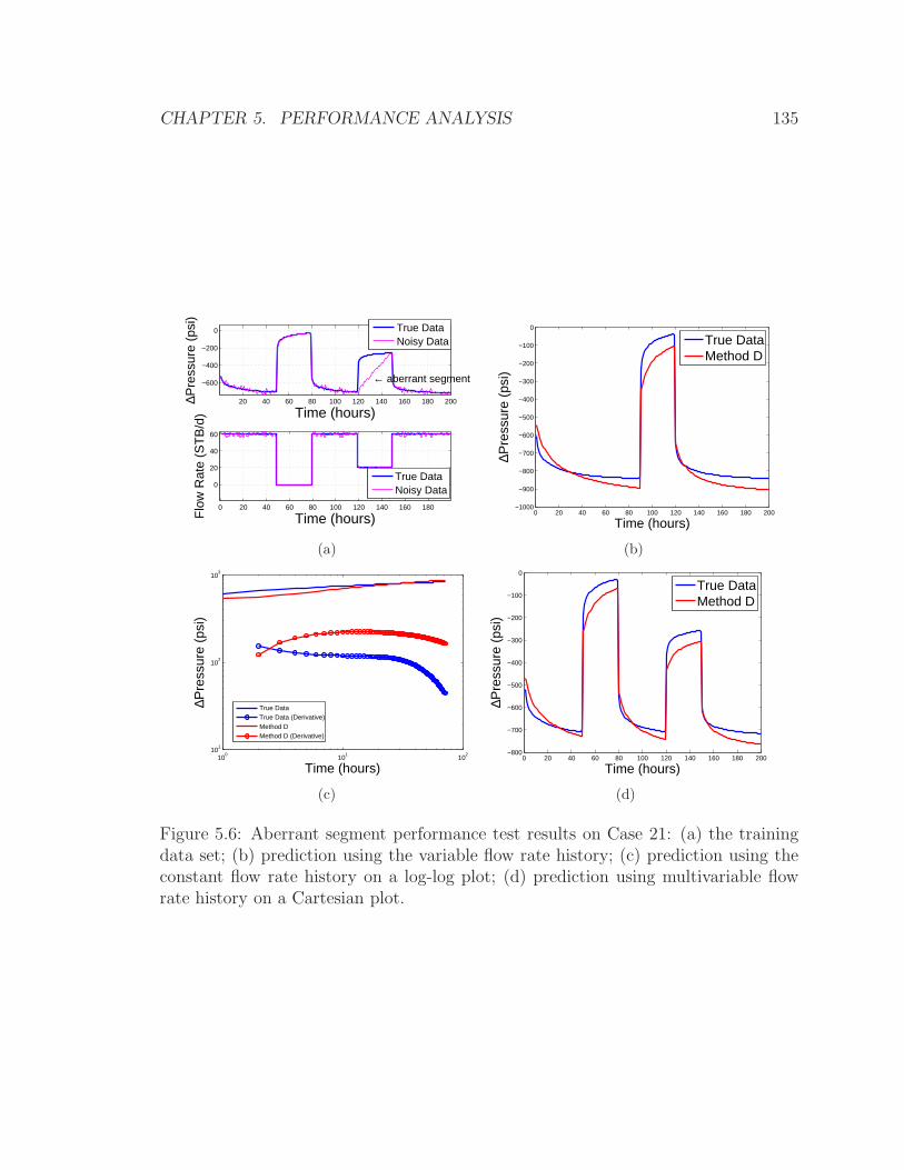
CHAPTER 5. PERFORMANCE ANALYSIS 135
20 40 60 80 100 120 140 160 180 200
−600
−400
−200
0
← aberrant segment
Time (hours)
∆Pre
ssur
e (p
si)
True DataNoisy Data
0 20 40 60 80 100 120 140 160 180
0
20
40
60
Time (hours)Flo
w R
ate
(ST
B/d
)
True DataNoisy Data
(a)
0 20 40 60 80 100 120 140 160 180 200−1000
−900
−800
−700
−600
−500
−400
−300
−200
−100
0
Time (hours)
∆Pre
ssur
e (p
si)
True DataMethod D
(b)
100
101
102
101
102
103
Time (hours)
∆Pre
ssur
e (p
si)
True DataTrue Data (Derivative)Method DMethod D (Derivative)
(c)
0 20 40 60 80 100 120 140 160 180 200−800
−700
−600
−500
−400
−300
−200
−100
0
Time (hours)
∆Pre
ssur
e (p
si)
True DataMethod D
(d)
Figure 5.6: Aberrant segment performance test results on Case 21: (a) the trainingdata set; (b) prediction using the variable flow rate history; (c) prediction using theconstant flow rate history on a log-log plot; (d) prediction using multivariable flowrate history on a Cartesian plot.

CHAPTER 5. PERFORMANCE ANALYSIS 136
20 40 60 80 100 120 140 160 180 200
−600
−400
−200
0
← data removed
Time (hours)
∆Pre
ssur
e (p
si)
True DataNoisy Data
20 40 60 80 100 120 140 160 180 200
0
20
40
60
Time (hours)Flo
w R
ate
(ST
B/d
)
True DataNoisy Data
(a)
0 20 40 60 80 100 120 140 160 180 200−900
−800
−700
−600
−500
−400
−300
−200
−100
0
Time (hours)
∆Pre
ssur
e (p
si)
True DataMethod D
(b)
100
101
102
101
102
103
Time (hours)
∆Pre
ssur
e (p
si)
True DataTrue Data (Derivative)Method DMethod D (Derivative)
(c)
0 20 40 60 80 100 120 140 160 180 200−800
−700
−600
−500
−400
−300
−200
−100
0
Time (hours)
∆Pre
ssur
e (p
si)
True DataMethod D
(d)
Figure 5.7: Aberrant segment performance test results on Case 22: (a) the trainingdata set; (b) prediction using the variable flow rate history; (c) prediction using theconstant flow rate history on a log-log plot; (d) prediction using multivariable flowrate history on a Cartesian plot.

CHAPTER 5. PERFORMANCE ANALYSIS 137
reduces as the aberrancy becomes more severe. The convolution kernel method may
handle moderate aberrant segments with a resulting small deviation in the prediction,
whereas a severe aberrant segment would affect the prediction in absolute value while
retaining the overall shape of the true response. A preremoval of the aberrant segment
improves the precision of the data mining algorithm significantly.
5.3 Partial Production History
In a PDG data set, it is common to see a period of production history that is missing.
The data missing might be due to many reasons, such as the unavailability of the
measuring devices, or unexpected loss in the data storage, etc. In this case, the
data mining algorithm will face a partial production history. In this section, the
performance of the data mining algorithm working with a partial production history
is discussed.
In order to investigate the performance of the convolution kernel method working
with an incomplete data set, we first formed a semireal data set, as shown in Fig. 5.8.
We used this data set as the complete data set, and then used only the data in the
range of [100h, 300h] (data in the red box) as an incomplete data set to conduct the
tests.
The work flow of the test is as follows.
1. Construct a synthetic pressure, flow rate data set, and add 3% artificial noise
(normally distributed) to both the pressure and the flow rate data. This will
be the original complete data set as shown in Fig. 5.8.
2. Extract a part of the data in the range of [100h, 300h] from the original com-
plete data set (with artificial noise) as the training data set. Apply convolution
kernelized data mining algorithms (Method D) to learn the data set until con-
vergence.
3. Feed the data mining algorithm with the training variable flow rate history
(without outliers nor noise) and collect the prediction from the data mining
algorithm.

CHAPTER 5. PERFORMANCE ANALYSIS 138
0 50 100 150 200 250 300−1500
−1000
−500
0
500
Time (hours)
∆Pre
ssur
e (p
si)
True DataNoisy Data
0 50 100 150 200 250 300
0
50
100
Time (hours)Flo
w R
ate
(ST
B/d
)
True DataNoisy Data
Figure 5.8: The original complete semireal data set for the performance test of theconvolution kernel method working with partial production history.
4. Compare the predicted pressure data (from Step 3) with the synthetic pressure
data without noise (from Step 1).
5. Feed the data mining algorithm with a constant flow rate history (without
outliers nor noise) and collect the predicted pressures from the data mining
algorithm.
6. Construct a synthetic pressure according to the constant flow rate from Step 5
using the same wellbore/reservoir model from Step 1.
7. Compare the predicted pressure data (from Step 5) with the synthetic pressure
data (from Step 6).
This work flow was performed in Test Case 23, listed in Table 5.3.
Fig. 5.9 demonstrates the results of Case 23. The pressure reproduction of the
training flow rate is shown in Fig. 5.9(a). In the figure, it seems that the pressure was
reproduced well. The pressure near 170h and the pressure in the range of [200h, 220h]
have slight deviation from the true data. However, the good result was not retained

CHAPTER 5. PERFORMANCE ANALYSIS 139
Table 5.3: Test case for partial production history performance analysis
Test Case # Test Case Characteristics
23 Infinite-acting radial flow + wellbore effect + skin + constantpressure boundary; use the data from 100h to 300h as thetraining data to simulate the situation in which the first 100hproduction history is missing; no effective rate readjustmentwas made.
in the pressure prediction to the constant flow rate history, demonstrated by a log-log
plot in Fig. 5.9(b). In the log-log plot, the pressure prediction is still close to that
of the true data. However, the derivative curve shows that the prediction misses the
wellbore effect and infinite-acting radial flow. For the boundary, the prediction not
only deviated from the absolute value of the true answer, it also mistakenly replaced
the constant pressure boundary behavior by a pseudosteady state boundary behavior.
These errors are caused by the missing production history, especially, the missing
flow rate history in the first 100 hours. This could be explained by the construction
of the “parts” of the convolution kernel. Referring to Section 4.2, each part is defined
by a flow rate change event. Also in the convolution kernel method, in order to avoid
the breakpoint detection, each sampling point is treated as a flow rate change event.
Therefore, missing the flow rate history for the first 100 hours means that the first
part of the training data is defined by the sampling point at 100h. Because no earlier
part is available before this part, this part was treated as representative of the first
100 hours, which means that the flow rate in the first 100 hours was treated constant
as the value at 100h. Referring to Fig. 5.8, the flow rate at 100h is not representative
of the first 100 hours due to a nearly 50 hours shut-in from around 50h to around
75h. The dramatic change of the flow rate in the first 100 hours causes the error in
the well/reservoir model extraction by the data mining algorithm.
An approach to fix this problem is to reconstruct the flow rate data in the miss-
ing period using the PDG pressure data, as discussed in the literature review (Sec-
tion 2.2.3). However, this method would not work when the PDG pressure data is also
not available – actually, this is very possible when an unexpected data loss happens.
We proposed an alternative solution to handle this problem, namely effective rate

CHAPTER 5. PERFORMANCE ANALYSIS 140
100 120 140 160 180 200 220 240 260 280 300−1100
−1000
−900
−800
−700
−600
−500
−400
Time (hours)
∆Pre
ssur
e (p
si)
True DataMethod D
(a)
100
101
102
101
102
103
Time (hours)
∆Pre
ssur
e (p
si)
True DataTrue Data (Derivative)Method DMethod D (Derivative)
(b)
Figure 5.9: Partial production history performance test results on Case 23 (withouteffective rate correction): (a) pressure reproduction to the training flow rate history;(b) prediction using the constant flow rate history on a log-log plot
readjustment. In a reservoir, the cumulative production is usually well documented.
With this cumulative oil production, we may calculate the effective rate as:
qeff =Q(1)
t(1)(5.1)
where t(1) is the first available time in the partial data set, and the Q(1) is the cumu-
lative oil production at t(1).
We then replace q(1) (the flow rate at t(1)) with this effective flow rate. That
is, the effective flow rate is selected to construct the first part of the partial data,
representing the flow rate of the whole missing period. Using the concept of the
effective rate, a new work flow was formed as follows:
1. Construct a synthetic pressure, flow rate data set, and add 3% artificial noise
(normally distributed) to both the pressure and the flow rate data. This will
be the original complete data set as shown in Fig. 5.8.
2. Extract the data in the range of [100h, 300h] in the original complete data
set (with artificial noise) as the training data set. Calculate the effective
flow rate for the first 100h. Replace the first flow rate (flow rate at
CHAPTER 5. PERFORMANCE ANALYSIS 141
100h) with the effective rate. Apply the convolution kernelized data mining
algorithm (Method D) to learn the data set until convergence.
3. Feed the data mining algorithm with the training variable flow rate history
(without outliers nor noise) and collect the prediction from the data mining
algorithm.
4. Compare the predicted pressure data (from Step 3) with the synthetic pressure
data without noise (from Step 1).
5. Feed the data mining algorithm with a constant flow rate history (without
outliers nor noise) and collect the predicted pressures from the data mining
algorithm.
6. Construct a synthetic pressure according to the constant flow rate from Step 5
using the same wellbore/reservoir model from Step 1.
7. Compare the predicted pressure data (from Step 5) with the synthetic pressure
data (from Step 6).
This work flow was applied to Test Case 24, listed in Table 5.4.
Table 5.4: Test case for partial production history performance analysis
Test Case # Test Case Characteristics
24 Infinite-acting radial flow + wellbore effect + skin + constantpressure boundary; use the data from 100h to 300h as thetraining data to simulate the situation in which the first 100hproduction history is missing; effective rate readjustment wasmade.
Fig. 5.10 demonstrates the results of Case 24. The pressure reproduction to the
training flow rate is shown in Fig. 5.10(a). The pressure reproduction is very close
to the true data. Compared to Fig. 5.9(a), the slight deviations near 170h and the
pressure in [200h, 220h] are not apparent in Fig. 5.10(a). Also, in the log-log plot
of Fig. 5.10(b) the pressure derivative curve prediction to the constant flow rate is

CHAPTER 5. PERFORMANCE ANALYSIS 142
much improved compared that in Fig. 5.9(b). The data mining algorithm captured
the infinite-acting radial flow and the constant pressure boundary. A deviation exists
only in the wellbore storage region. These improvements show that the pressure
prediction would be improved if the effective rate readjustment is imposed.
100 120 140 160 180 200 220 240 260 280 300−1100
−1000
−900
−800
−700
−600
−500
−400
−300
Time (hours)
∆Pre
ssur
e (p
si)
True DataMethod D
(a)
100
101
102
100
101
102
103
Time (hours)∆P
ress
ure
(psi
)
True DataTrue Data (Derivative)Method DMethod D (Derivative)
(b)
Figure 5.10: Partial production history performance test results on Case 24 (witheffective rate correction): (a) pressure reproduction to the training flow rate history;(b) prediction using the constant flow rate history on a log-log plot
In addition to the effective rate correction that was discussed above, we also inves-
tigated another kind of correction, namely effective time correction, to accommodate
the incomplete production history. In the effective time correction, instead of chang-
ing the flow rate, we readjusted the time of the incomplete production history. First,
we calculated the effective start time by Eq. 5.2.
teff =Q(1)
q(1)(5.2)
where q(1) is the first available flow rate in the partial data set. Then, we shift the
incomplete production data set to the effective start time using Eq. 5.3
(
t(i))′= t(i) −
(
t(1) − teff)
where i = 1, . . . , Np (5.3)
In this effective time correction, we tried to use the first known flow rate as
the constant average flow rate in the unknown production period, and adjusted the

CHAPTER 5. PERFORMANCE ANALYSIS 143
production time to satisfy the balance between the constant average flow rate and the
accumulated production rate. The reason we imposed this effective time correction
came from the fact that the effective rate correction changed the first flow rate without
changing the first pressure leading to an unmatched flow-rate-pressure pair.
However, the test result did not meet our expectation. Applying this effective
time correction on Case 24, the results are shown in Fig. 5.11. Fig. 5.11(a) shows the
reproduction of the training data set which is an incomplete production history. The
reproduction is very close to the training pressure. However, the prediction to the
constant flow rate history on the log-log plot demonstrated in Fig. 5.11(b) suggests
another story. Apparently, the prediction misses the early stage (wellbore effect) and
the late stage (boundary effect) of the pressure transient. Only the infinite-acting
radial flow period is close to the true answer, yet still has an obvious deviation. These
results suggest that the effective time correction does not improve the prediction result
as well as the effective rate correction does, at least for Case 24. Further study might
be required to investigate the feasibility of the effective time correction thoroughly.
0 50 100 150 200 250−1100
−1000
−900
−800
−700
−600
−500
−400
Time (hours)
∆Pre
ssur
e (p
si)
True DataMethod D
(a)
100
101
102
101
102
103
Time (hours)
∆Pre
ssur
e (p
si)
True DataTrue Data (Derivative)Method DMethod D (Derivative)
(b)
Figure 5.11: Partial production history performance test results on Case 24 (witheffective time correction): (a) pressure reproduction to the training flow rate history;(b) prediction using the constant flow rate history on a log-log plot
Test Cases 23 and 24 in this section demonstrate the performance of the coonvo-
lution kernel method working in the condition of partial production history without
and with the effective rate readjustment respectively. Case 23 shows that the missing

CHAPTER 5. PERFORMANCE ANALYSIS 144
production history (especially the missing flow rate history) affects the accuracy of
the prediction. However, by imposing the effective rate readjustment as in Case 24,
the effect of the missing period may be decreased to an acceptable level.
5.4 Unknown Initial Pressure
Similar to the missing production history, initial pressure identification is also a com-
monly seen problem in the PDG data analysis. In a real production, the initial
pressure of the reservoir might be unknown due to the long time elapsed since the
initial production, or due to the transition of the ownership of the reservoir. Even
though the initial pressure may be on file, it could be inappropriate due to subse-
quent shut-ins. All of these difficulties require the convolution kernel method to face
a unknown or inappropriate initial pressure, which is discussed in this section.
In order to address this problem, we first constructed a semireal data set, and
then shifted the initial pressure by 100 psi to form a training data to simulate the
scenario of inappropriate initial pressure, as shown in Fig. 5.12. This training data
set was the training data set for both Cases 25 and 26 discussed in this section. When
an inappropriate initial pressure is proposed, there would be an offset in the pressure
change compared to the true data. For example, in Fig. 5.12, the initial pressure of
the training data is set 100 psi more than that of the true data, leading to a constant
offset of 100 psi globally.
The study then investigated the effect of this inappropriate initial pressure by
using the work flow as follows.
1. Construct a synthetic pressure, flow rate data set.
2. Make the initial pressure 100 psi more than the true initial pressure, and add
3% artificial noise (normally distributed) to both the pressure and the flow rate
data. This will be the training data set with a wrong initial pressure. Apply
convolution kernelized data mining algorithms (Method D) to learn the data
set until convergence.

CHAPTER 5. PERFORMANCE ANALYSIS 145
0 50 100 150 200−1000
−500
0
Time (hours)∆P
ress
ure
(psi
)
True DataNoisy Data
0 50 100 150 2000
20
40
60
80
Time (hours)Flo
w R
ate
(ST
B/d
)
True DataNoisy Data
Figure 5.12: The original true semireal data set and the training data for the perfor-mance test of the convolution kernel method working with a wrong initial pressure.The training data set has a offset to the true data due to the inappropriate initialpressure settings.
3. Feed the data mining algorithm with the training variable flow rate history
(without noise) and collect the prediction from the data mining algorithm.
4. Compare the predicted pressure data (from Step 3) with the synthetic pressure
data without noise (from Step 1).
5. Feed the data mining algorithm with a constant flow rate history (without noise)
and collect the predicted pressures from the data mining algorithm.
6. Construct a synthetic pressure according to the constant flow rate from Step 5
using the same wellbore/reservoir model from Step 1.
7. Compare the predicted pressure data (from Step 5) with the synthetic pressure
data (from Step 6).
The work flow was performed on Test Case 25, as listed in Table 5.5.
Fig. 5.13 shows the results of Case 25. The pressure reproduction to the training
flow rate history is shown in Fig. 5.13(a). Despite a global offset of 100 psi in the
training pressure data, the pressure reproduction still tried to return to the correct

CHAPTER 5. PERFORMANCE ANALYSIS 146
Table 5.5: Test case for unknown initial pressure performance analysis
Test Case # Test Case Characteristics
25 Infinite-acting radial flow + wellbore effect + skin + constantpressure boundary; no optimization on the initial pressure.
track of the true data beginning at 100 hours of the prediction. However, the pressure
prediction in the last 100 hours still shows a deviation of around 100 psi, which is
a reflection of the effect of the inappropriate initial pressure. The log-log plot in
Fig. 5.13(b) demonstrates the pressure prediction to a constant flow rate history. The
derivative curves show that the pressure prediction deviates from the true answer in
the infinite-acting radial flow region. These plots show that the inappropriate initial
pressure results in inaccuracy in the pressure prediction.
0 20 40 60 80 100 120 140 160 180 200−1000
−900
−800
−700
−600
−500
−400
−300
−200
−100
0
Time (hours)
∆Pre
ssur
e (p
si)
True DataMethod D
(a)
100
101
102
100
101
102
103
104
Time (hours)
∆Pre
ssur
e (p
si)
True DataTrue Data (Derivative)Method DMethod D (Derivative)
(b)
Figure 5.13: Unknown initial pressure performance test results on Case 25: (a) pre-diction using the variable flow rate history; (b) prediction using the constant flowrate history on a log-log plot.
To solve the problem of unknown initial pressure, we imposed an outer iteration
on the initial pressure during the data mining process. In this way, the initial pressure
is treated an unknown argument in the optimization iterations. In each optimization
iteration, the initial pressure is used to regenerate the training data set on which the
data mining algorithm is applied. When the data mining process finished, we make
the data mining algorithm reproduce the pressure to the training flow rate. There

CHAPTER 5. PERFORMANCE ANALYSIS 147
is a difference between the pressure reproduction and the training pressure. When
the difference is small enough, we believe that the pressure reproduction is converged
to the training pressure, and hence obtain the initial pressure. Otherwise, the initial
pressure would be updated using the pressure difference for the next iteration. This
logic could be expressed using the pseudocode in Algorithm 4.
Algorithm 4 Data mining coupled with optimization on initial pressure
p[0]i = max
p(1), . . . , p(Np)
use the max pressure as the initial guess of the initialpressureiter = 0 initialize the iteration counterwhile iter < MAX ITER doUse the p
[iter]i as the initial pressure to update the training data set, obtaining
y[iter].Apply the data mining algorithm on the new training data setUse the data mining result to obtain the pressure reproduction (ypred[iter]) to thetraining flow rate historyif ypred[iter] is convergent to y[iter] thenreturn p
[iter]i
end ifUpdate p
[iter+1]i
iter = iter + 1 update the iteration counterend whilereturn p
[MAX ITER]i
With the Algorithm 4, a new work flow was formed as follows.
1. Construct a synthetic pressure, flow rate data set.
2. Make the initial pressure 100 psi more than the true initial pressure, and add
3% artificial noise (normally distributed) to both the pressure and the flow rate
data. This will be the training data set with a wrong initial pressure. Apply
convolution kernelized data mining with initial pressure optimization
algorithm (Algorithm 4) to learn the data set until convergence.
3. Feed the data mining algorithm with the training variable flow rate history
(without noise) and collect the prediction from the data mining algorithm.

CHAPTER 5. PERFORMANCE ANALYSIS 148
4. Compare the predicted pressure data (from Step 3) with the synthetic pressure
data without noise (from Step 1).
5. Feed the data mining algorithm with a constant flow rate history (without noise)
and collect the predicted pressures from the data mining algorithm.
6. Construct a synthetic pressure according to the constant flow rate from Step 5
using the same wellbore/reservoir model from Step 1.
7. Compare the predicted pressure data (from Step 5) with the synthetic pressure
data (from Step 6).
The new work flow was performed on Test Case 26, as listed in Table 5.6.
Table 5.6: Test case for unknown initial pressure analysis
Test Case # Test Case Characteristics
26 Infinite-acting radial flow + wellbore effect + skin + constantpressure boundary; optimize the initial pressure as the outerloop over the data mining algorithm.
The results of Case 26 are demonstrated in Fig. 5.14. Fig, 5.14(a) shows the
pressure reproduction to the training flow rate. The pressure was reproduced well
compared to the true data. The log-log plot in Fig. 5.14(b) shows the pressure predic-
tion to the constant flow rate history. The derivative curves show that the pressure
prediction captures well the infinite-acting radial flow and the boundary, despite a
slight deviation in the wellbore effect region. The improvement in these plots suggests
that an optimization algorithm outside the data mining process helps to estimate the
appropriate initial pressure, and hence improve the accuracy of the pressure predic-
tion. In this optimization process, the data mining algorithm is actually used as a
black box whose input is the new guess of initial pressure, and whose output is the
pressure reproduction to the training flow rate history.
To sum up, in this section Case 25 demonstrated the effect of the inappropriate
initial pressure in the pressure prediction, while Case 26 suggested that an optimiza-
tion algorithm on the initial pressure outside the data mining algorithm would help to

CHAPTER 5. PERFORMANCE ANALYSIS 149
0 20 40 60 80 100 120 140 160 180 200−800
−700
−600
−500
−400
−300
−200
−100
0
Time (hours)
∆Pre
ssur
e (p
si)
True DataMethod D
(a)
100
101
102
101
102
103
Time (hours)
∆Pre
ssur
e (p
si)
True DataTrue Data (Derivative)Method DMethod D (Derivative)
(b)
Figure 5.14: Unknown initial pressure performance test results on Case 26: (a) pre-diction using the variable flow rate history; (b) prediction using the constant flowrate history on a log-log plot.
find the appropriate initial pressure and improve the precision of the pressure predic-
tion. As a byproduct, these tests show another application of data mining algorithm
to find the appropriate initial pressure by using the data mining algorithm as a black
box.
5.5 Sampling Frequency
Sampling frequency is an important property of the data set. The sampling rate of
the data set may be affected by factors in both the hardware and the software. On
one hand, each PDG device may be programmed to record at a specific frequency,
hence deciding the sampling frequency of the raw measurement. On the other hand,
when the data set is large due to high frequency of the measurement, the data set is
usually resampled in a preprocessing process due to the consideration of performance.
As discussed in Section 4.3, the richness of the data fundamentally affects the data
mining process in the pseudo-high-dimensional space. In this way, the sampling
frequency also affects the precision of the data mining because the sampling frequency
is actually the data density of the data set deciding the richness of the data given
a specific period. The performance of the convolution kernel method working in

CHAPTER 5. PERFORMANCE ANALYSIS 150
different sampling frequencies is investigated in this section.
0 50 100 150 200−1500
−1000
−500
0
Time (hours)
∆Pre
ssur
e (p
si)
True DataNoisy Data
0 50 100 150 200
0
50
100
Time (hours)Flo
w R
ate
(ST
B/d
)
True DataNoisy Data
Figure 5.15: The original complete semireal data set for the sampling frequency testsfor Cases 27-30.
To test the effect of the sampling frequency, we constructed a data set as shown
in Fig. 5.15. In this data set, there are 200 hours of data sampled by 400 points.
This set will be the base data set for Test Cases 27-30. Test Cases 27-30 resampled
the data set in Fig. 5.15 with different frequency to observe the behaviors of the
data mining algorithm. The detailed characterization of these test cases is listed in
Table 5.7. According to the description, the sampling frequency for Cases 27-30 are
1 point per 4 hours, 1 point per 2 hours, 1 point per hour, and 1 point per half hour
respectively. These test cases were conducted with the work flow as follows.
1. Construct a synthetic pressure, flow rate data set, add 3% artificial noise (nor-
mally distributed) to both the pressure and the flow rate.
2. Resample the data set from Step 1 with a given sampling frequency to form a
training data set. Apply the convolution kernel method to learn the training
data set until convergence.
3. Feed the data mining algorithm with the training variable flow rate history
(without noise) and collect the prediction from the data mining algorithm.

CHAPTER 5. PERFORMANCE ANALYSIS 151
Table 5.7: Test cases for sampling frequency performance analysis
Test Case # Test Case Characteristics
27 Infinite-acting radial flow + wellbore effect + skin + constantpressure boundary; 200 hour data sampled by 50 points.
28 Infinite-acting radial flow + wellbore effect + skin + constantpressure boundary; 200 hour data sampled by 100 points.
29 Infinite-acting radial flow + wellbore effect + skin + constantpressure boundary; 200 hour data sampled by 200 points.
30 Infinite-acting radial flow + wellbore effect + skin + constantpressure boundary; 200 hour data sampled by 400 points.
4. Compare the predicted pressure data (from Step 3) with the synthetic pressure
data without noise (from Step 2).
5. Feed the data mining algorithm with a constant flow rate history (without noise)
and collect the predicted pressures from the data mining algorithm.
6. Construct a synthetic pressure according to the constant flow rate from Step 5
using the same wellbore/reservoir model from Step 1.
7. Compare the predicted pressure data (from Step 5) with the synthetic pressure
data (from Step 6).
Fig. 5.16 shows the pressure reproductions to the training data set in Cases 27-
30. Recall Case 27 has the least frequent sampling, the training data set of Case
27 is the smallest in the four. Fewer data leads to an incomplete kernel function
basis, which explains the deviation in the corners in Fig. 5.16(a). Similarly, some
slight deviations also exist in Case 28, as shown in Fig. 5.16(b). Compared with the
pressure reproductions in Cases 27 and 28, those in Cases 29 and 30, demonstrated
in Figs. 5.16(c) and 5.16(d) are so close to the true data that the true data are barely
seen behind the prediction. This is because the more frequent sampling brought more
data in the training data sets in Cases 29 and 30.
The effect of the sampling frequency can be seen more clearly in the log-log plots
in Fig. 5.17. Comparing the pressure derivative curves in the four log-log plots, it is

CHAPTER 5. PERFORMANCE ANALYSIS 152
0 20 40 60 80 100 120 140 160 180 200−1200
−1000
−800
−600
−400
−200
0
Time (hours)
∆Pre
ssur
e (p
si)
True DataMethod D
(a)
0 20 40 60 80 100 120 140 160 180 200−1200
−1000
−800
−600
−400
−200
0
Time (hours)
∆Pre
ssur
e (p
si)
True DataMethod D
(b)
0 20 40 60 80 100 120 140 160 180 200−1200
−1000
−800
−600
−400
−200
0
Time (hours)
∆Pre
ssur
e (p
si)
True DataMethod D
(c)
0 20 40 60 80 100 120 140 160 180 200−1200
−1000
−800
−600
−400
−200
0
Time (hours)
∆Pre
ssur
e (p
si)
True DataMethod D
(d)
Figure 5.16: The pressure reproduction to the training flow rate history in (a) Case27, (b) Case 28, (c) Case 29, and (d) Case 30.

CHAPTER 5. PERFORMANCE ANALYSIS 153
apparent that the prediction improves consistently from Case 27 in Fig. 5.17(a) to
Case 30 in Fig. 5.17(d). In Fig. 5.17(a), the prediction captures the overall trend but
loses the details in the wellbore effect and the infinite-acting radial flow regions. In
Fig. 5.17(b), the infinite-acting radial flow region begins to approach the true answer,
while in Fig. 5.17(c) and 5.17(d) the infinite-acting radial flow are captured.
In Fig. 5.17, three observations attract our attention. First, in Fig. 5.17(a), al-
though the prediction loses the infinite-acting radial flow region, it captures the con-
stant pressure boundary very well. From the log-log plot we may see that in the
synthetic model, it takes at least 30 hours for the pressure to respond to the bound-
ary effect. Hence, more than 3/4 of the data (200 hours in total) lay in the region
of the boundary effect, leaving less than 1/4 of the data for the rest of the transient.
Considering there were only 50 points in total in Case 27, actually only around 10
points were involved in the prediction for the infinite-acting radial flow region, while
there were around 40 points for the boundary effect region. Therefore, the difference
for the prediction in the infinite-acting radial flow region and the boundary effect
region are still caused by the richness of the data. Secondly, comparing Fig. 5.17(c)
with Fig. 5.17(d), Case 30 has a better prediction in the infinite-acting radial flow
region, especially the connection to the boundary effect region, while Case 30 deviates
from the wellbore storage region. This is because the wellbore storage effect is a short
period feature dominating the derivative curve for only a few hours at the beginning.
However, the infinite-acting radial flow and the boundary effect are long lasting be-
haviors. Hence, when the data are more numerous, the learning algorithm prefers to
focus more on the lasting behavior rather than the short term behavior, leading to
the slight deviation in the wellbore storage region and a small improvement in the
infinite-acting radial flow region in Fig. 5.17(d). Finally, appropriate resampling did
not decrease much the precision of the prediction. Such as in Case 29, the size of the
training data set was half that of the original data set. However, the accuracy of the
prediction was not decreased. This implies the feasibility of resampling the data set
to improve the speed of the computation.
After the tests of Cases 27-30, we may conclude that the convolution kernel method
is able to work under different sampling frequencies. Too infrequent sampling leads

CHAPTER 5. PERFORMANCE ANALYSIS 154
100
101
102
101
102
103
Time (hours)
∆Pre
ssur
e (p
si)
True DataTrue Data (Derivative)Method DMethod D (Derivative)
(a)
100
101
102
101
102
103
Time (hours)
∆Pre
ssur
e (p
si)
True DataTrue Data (Derivative)Method DMethod D (Derivative)
(b)
100
101
102
101
102
103
Time (hours)
∆Pre
ssur
e (p
si)
True DataTrue Data (Derivative)Method DMethod D (Derivative)
(c)
100
101
102
101
102
103
Time (hours)
∆Pre
ssur
e (p
si)
True DataTrue Data (Derivative)Method DMethod D (Derivative)
(d)
Figure 5.17: The pressure reproduction to the constant flow rate history in (a) Case27, (b) Case 28, (c) Case 29, and (d) Case 30.

CHAPTER 5. PERFORMANCE ANALYSIS 155
to deviation in the prediction due to the lack of data. However, appropriate sampling
retains the precision of the prediction as well as accelerates the computation of the
prediction. It is worth some further exploration in future study as to what is the best
sampling/resampling frequency.
5.6 Evolution of Learning
Section 5.5 discussed the effect of the sampling frequency of the data set. However,
when the sampling frequency is fixed, the richness of the data set will depend on the
total time span of the data. A typical scenario relevant to the effect of the time span
is in a real-time measurement. The measurements are fed in more and more as time
elapses. Considering the data mining algorithm digs information only from the data
that has, different time spans of the data are expected to bring different information
to the data mining algorithm. Hence, in a real-time data analysis, an evolution of
the learning and the prediction will be seen along with the growth of the time span
of the training data. In this section, we demonstrate an evolution learning process,
and discuss the effect of the time span.
In order to investigate the issue, a semireal case was constructed, as shown in
Fig. 5.18. This data set covers 200 hours sampled by 200 points. Four test cases,
namely Cases 31-34 were then constructed by spanning different lengths of the data
set. The characterization of the four test cases is listed in Table 5.8. Cases 31-34
spanned the first 20, 50, 100, 200 hours of the original data set to simulate a real-time
progress of the data acquisition. These four tests were conducted using the work flow
as follows.
1. Construct a synthetic pressure, flow rate data set, add 3% artificial noise (nor-
mally distributed) to both the pressure and the flow rate.
2. Extract a piece of the data set from Step 1 with a given length of period to
form the training data set. Apply the convolution kernel method to learn the
training data set until convergence.

CHAPTER 5. PERFORMANCE ANALYSIS 156
0 50 100 150 200−800
−600
−400
−200
0
Time (hours)
∆Pre
ssur
e (p
si)
True DataNoisy Data
0 50 100 150 200
0
20
40
60
Time (hours)Flo
w R
ate
(ST
B/d
)
True DataNoisy Data
Figure 5.18: The original complete semireal data set for evolution learning tests forCases 31-34.
Table 5.8: Test cases for evolution learning performance analysis
Test Case # Test Case Characteristics
31 Infinite-acting radial flow + wellbore effect + skin + constantpressure boundary; first 25 hour data.
32 Infinite-acting radial flow + wellbore effect + skin + constantpressure boundary; first 50 hour data.
33 Infinite-acting radial flow + wellbore effect + skin + constantpressure boundary; first 100 hour data.
34 Infinite-acting radial flow + wellbore effect + skin + constantpressure boundary; first 200 hour data.

CHAPTER 5. PERFORMANCE ANALYSIS 157
3. Feed the data mining algorithm with the training variable flow rate history
(without noise) and collect the prediction from the data mining algorithm.
4. Compare the predicted pressure data (from Step 3) with the synthetic pressure
data without noise (from Step 2).
5. Feed the data mining algorithm with a constant flow rate history (without noise)
and collect the predicted pressures from the data mining algorithm.
6. Construct a synthetic pressure according to the constant flow rate from Step 5
using the same wellbore/reservoir model from Step 1.
7. Compare the predicted pressure data (from Step 5) with the synthetic pressure
data (from Step 6).
Fig. 5.19 shows the pressure reproduction to the training flow rate history in
Cases 31-34. As there are only 25 hours of data (25 points) in Case 31, the pressure
reproduction has a slight deviation compared to the true data in Fig. 5.19(a) due
to the lack of data. For Cases 32-34, the pressure reproductions all seem good, as
demonstrated in Figs. 5.19(b) to 5.19(d).
However, log-log plots of the pressure prediction to the constant flow rate history
reveals another side of the story, as demonstrated in Fig. 5.20. The derivative curves
in the log-log plots suggest an evolution of the pressure prediction – in Fig. 5.20(a), the
pressure prediction only captures the wellbore effect and the infinite-acting radial flow,
while in Fig. 5.20(d) the prediction captures nearly all features of the well/reservoir
model. The whole evolution demonstrates the learning process of the data mining
algorithm. In the synthetic model, it requires at least 30 hours for the pressure to
respond to the constant pressure boundary. However, in Case 31, only the first 25
hour data were fed to the learning algorithm, so what the data mining algorithm saw
was only the wellbore effect, skin effect and the infinite-acting radial flow. That is
why the prediction in Fig. 5.20(a) does not show the constant pressure boundary in
the derivative curve. In Case 32, because the first 50 hours of data were provided,
it became possible for the data mining algorithm to detect the constant pressure

CHAPTER 5. PERFORMANCE ANALYSIS 158
0 5 10 15 20 25−440
−430
−420
−410
−400
−390
−380
−370
−360
−350
Time (hours)
∆Pre
ssur
e (p
si)
True DataMethod D
(a)
0 5 10 15 20 25 30 35 40 45 50−500
−450
−400
−350
−300
−250
−200
−150
−100
−50
0
Time (hours)
∆Pre
ssur
e (p
si)
True DataMethod D
(b)
0 10 20 30 40 50 60 70 80 90 100−500
−450
−400
−350
−300
−250
−200
−150
−100
−50
0
Time (hours)
∆Pre
ssur
e (p
si)
True DataMethod D
(c)
0 20 40 60 80 100 120 140 160 180 200−800
−700
−600
−500
−400
−300
−200
−100
0
Time (hours)
∆Pre
ssur
e (p
si)
True DataMethod D
(d)
Figure 5.19: The pressure reproduction to the training flow rate history in (a) Case31, (b) Case 32, (c) Case 33, and (d) Case 34.

CHAPTER 5. PERFORMANCE ANALYSIS 159
boundary. Therefore, the derivative curve in Fig. 5.20(b) demonstrated a “dropping
tail” showing that the data mining algorithm had some detection of the boundary.
However, because the 50 hours was not sufficient for the boundary effect to develop
fully, the data mining algorithm was still not able to capture the boundary effect
accurately. Finally, in Cases 33 and 34, the timespan of the data set was long enough,
so the predictions in Figs. 5.20(c) and 5.20(d) captured the boundary effect.
Supposing that there was an engineer processing these data in real time, he or she
would see this evolution of the prediction as a reflection of the further and further
understanding of the well/reservoir by the data mining algorithm along with longer
and longer time span of the data set. Furthermore, supposing there is a reservoir that
has a production history of five years, the comparison between the prediction using
the first two years and the prediction using the first five years could demonstrate a
property change of the reservoir along with the continuing production. This implies
a new application of the data mining approach – observing the reservoir property
change by applying the data mining algorithm progressively to increasing time span
of the PDG data.
Cases 31-34 demonstrated the effect of the time span of the data set. Because
the data mining algorithm can only make prediction based on what it has learned
from the data, a short period of data leads to the absence of well/reservoir features
that require a long time to develop. Therefore, when the time span of the data set
grows, the prediction by the data mining algorithm also evolves. As a byproduct,
this evolution points to another potential application of the data mining algorithm
to evaluate the well/reservoir property change.
5.7 Summary
In this chapter, more realistic problems related to performance of the data mining
algorithm were discussed.
Sections 5.1 and 5.2 first discussed two kinds of commonly seen noise behaviors
of the PDG data, outliers and the aberrant segments. These two behaviors may lead
to more effect on the pressure prediction than the normal noise. The normal noise

CHAPTER 5. PERFORMANCE ANALYSIS 160
100
101
102
101
102
103
Time (hours)
∆Pre
ssur
e (p
si)
True DataTrue Data (Derivative)Method DMethod D (Derivative)
(a)
100
101
102
101
102
103
Time (hours)
∆Pre
ssur
e (p
si)
True DataTrue Data (Derivative)Method DMethod D (Derivative)
(b)
100
101
102
101
102
103
Time (hours)
∆Pre
ssur
e (p
si)
True DataTrue Data (Derivative)Method DMethod D (Derivative)
(c)
100
101
102
101
102
103
Time (hours)
∆Pre
ssur
e (p
si)
True DataTrue Data (Derivative)Method DMethod D (Derivative)
(d)
Figure 5.20: The pressure reproduction to the constant flow rate history in (a) Case31, (b) Case 32, (c) Case 33, and (d) Case 34.

CHAPTER 5. PERFORMANCE ANALYSIS 161
is usually pervasive and relatively small compared to the absolute value of the true
measurement. However, the outliers and the aberrant segments are more arbitrary
and far more deviated from the true measurement. Especially, the aberrant segments
are more problematic because the deviated data in the aberrant segments brings a
second logic interfering with the ability of the data mining algorithm to focus on
the true well/reservoir model. Nevertheless, the tests carried here still demonstrated
a good tolerance of the data mining algorithm to a moderate level of outliers and
aberrant segments. For severe outliers, Section 5.1 suggested that a low-noise flow rate
history may improve the precision of the prediction effectively despite the existence
of severe outliers in the pressure. Handling the severe aberrant segments, Section 5.2
demonstrated that a preremoval (just simple deletion, no interpolation required) of
the aberrant segment immediately corrected the prediction.
Incomplete production history and unknown initial pressure are another two prob-
lems, discussed in Sections 5.3 and 5.4. Sections 5.3 and 5.4 first showed the effect of
the pressure prediction by the data mining algorithm working in these two kinds of
situations. Thereafter two solutions were found for the incomplete production history
and the inappropriate initial pressure problems. For the partial production history,
an effective rate qeff was defined in Eq. 5.1. The effective rate, calculated using the
accumulative production, represents the average flow rate in the missing period. Also
for the unknown initial pressure, an algorithm optimizing the initial pressure out-
side the data mining process was proposed, as shown in Algorithm 4. The algorithm
utilizes the data mining process as a black box to search for the appropriate initial
pressure iteratively until the pressure prediction converges to the training data. The
test cases demonstrated the feasibility of the two methods.
Finally, Sections 5.5 and 5.6 discussed the effect of sampling frequency and the
time span of the data set. The sampling frequency and the overall time span together
decide the total number of data fed to the data mining algorithm. The test cases in
the two sections demonstrated that either low sampling frequency or short time span
of the data set would lead to the deviation of the final prediction. However, the mech-
anisms of the inaccurate prediction in the two situations are slightly different. For the
infrequent sampling, the whole data set is provided to the data mining algorithm, but

CHAPTER 5. PERFORMANCE ANALYSIS 162
not in detail due to the low sampling rate. Therefore, the data mining algorithm may
capture the overall trend but lose the accuracy in the feature details. However, for
the short time span, only part of the data is provided to the data mining algorithm,
so the data mining algorithm could only infer the well/reservoir model from a partial
data set missing the features that happen after the training time span. Nevertheless,
the deviation in the two scenarios are still consistent in the mathematical essence,
that is, the lack of training data leads to such an incomplete basis of kernel functions
K(
·,x(i))
that fβ (x) defined in Eq. 4.10 is not eligible to form an adequate esti-
mator of the true function f (refer to Section 4.3). As a result, Section 5.5 suggested
that an appropriate sampling rate that could provide sufficient basis kernel functions
should retain a good precision of the prediction as well as accelerate the performance
of the data mining process. Also, Section 5.6 illustrated the importance of the com-
pleteness of the data set and revealed a potential approach of observing the reservoir
property change using the data mining methods.
Along with the performance analysis, there were three important byproducts
worth future investigation. Firstly, the data mining method could be used as a black
box in an iterative optimization process to discover the appropriate initial pressure
of the reservoir. Secondly, resampling the PDG data set at an appropriate sampling
rate will not harm the prediction, but would improve the computational performance
of the data mining process. It would be a very helpful supplement if there is a way
to decide the appropriate sampling rate in advance of the training process. Finally,
applying the data mining to different lengths of the data time span results in an
evolution of the prediction. This could be utilized as a potential approach to observe
the property change of the well/reservoir model. All of these imply a future of wide
application of data mining methods in real practice.

Chapter 6
Rescalability
When the training data are numerous, the kernel matrix in the training equation,
Eq. 4.18 will be large. Recall that the computational cost of constructing the kernel
matrix is O(
N4p
)
(refer to Section. 4.6), so the large size of the matrix leads to a
low computational performance of the data mining process. To solve this problem,
a direct solution is to reduce the size of the data by resampling the original data
set with an appropriate sampling rate, as discussed in Section 5.5. An alternative
idea is to rescale the large kernel matrix into a series of block matrices, and solve the
training equation (Eq. 4.18) by solving a series of equations consisting of smaller block
matrices. In this chapter, the idea of rescaling the large kernel matrix into smaller
matrices is discussed. Based on the difference of the blocks that are used in the
training and prediction, two algorithms, namely block algorithm and advanced block
algorithm, are discussed in Sections 6.1 and 6.2 respectively. Finally, in Section 6.3, a
real field case is demonstrated, in which both the resampling and the advanced block
algorithm were applied.
163

CHAPTER 6. RESCALABILITY 164
6.1 Block Algorithm
To introduce the block algorithm, let us start from an easy example. Suppose that a
training data set has a total of 400 training samples. Hence, the training equation is:
Kβ = y (6.1)
where:
K =
Kij |Kij = K(
x(i),x(j))
, i, j = 1, . . . , 400
(6.2)
β = (β1, . . . , β400)T (6.3)
y =(
yobs(1), . . . , yobs(400))T
(6.4)
Then we divided the kernel matrix K ∈ ℜ400×400 into 200× 200 blocks. We have:
(
K11 K12
K21 K22
)(
β1
β2
)
=
(
y1
y2
)
(6.5)
where:
K11 =
Kij |Kij = K(
x(i),x(j))
, i, j = 1, . . . , 200
(6.6)
K12 =
Kij |Kij = K(
x(i),x(j))
, i = 1, . . . , 200, j = 201, . . . , 400
(6.7)
K21 =
Kij |Kij = K(
x(i),x(j))
, i = 201, . . . , 400, j = 1, . . . , 200
(6.8)
K22 =
Kij |Kij = K(
x(i),x(j))
, i, j = 201, . . . , 400
(6.9)
β1 = (β1, . . . , β200)T (6.10)
β2 = (β201, . . . , β400)T (6.11)
y1 =(
yobs(1), . . . , yobs(200))T
(6.12)
y2 =(
yobs(201), . . . , yobs(400))T
(6.13)
Then Eq. 6.5 may be expanded as:
K11β1 +K12β2 = y1 (6.14)

CHAPTER 6. RESCALABILITY 165
and
K21β1 +K22β2 = y2 (6.15)
Focusing on Eq. 6.14, we find that terms K11β1 and y1 are the terms related to
the first 200 samples only, while the term K12β2 is related to the last 200 samples.
Hence, Eq. 6.14 implies the first 200 pressure observations (y1) are affected not only
by the flow rate history in the first 200 samples (K11β1), but also by the flow rate
history in the last 200 samples (K12β2). This nonphysical implication inspired us to
conceive a reduction scenario: supposing that there are only the first 200 samples
for data mining, what will the training equation look like? Using the same variable
definition, the training equation will be:
K11β1 = y1 (6.16)
Comparing Eq. 6.15 with Eq. 6.16, the extra term in Eq. 6.15, K12β2, is caused
by additional basis kernel functions brought by the later 200 samples. Therefore,
assuming that the first 200 samples are eligible to form an adequate estimator of the
true function f (refer to Section 4.3), the extra term K12β2 should be able to be taken
out from Eq. 6.14. In this way, Eq. 6.14 will degrade to Eq. 6.16. Hence, β1 can be
solved as:
β1 = K−111 y1 (6.17)
Substitute Eq. 6.17 into Eq. 6.15, we have:
β2 = K−122 (y2 −K21β1) (6.18)
Using Eq. 6.17 and Eq. 6.18, the coefficient vector β is solved in two steps using
block matrices Kij instead of one step using the full matrix K.
To make this case general, for any kernel matrix K ∈ ℜ(u×v)×(u×v), u, v ∈ N, the
coefficient vector could be solved in v steps using the block matrices Kij ∈ ℜu×u,
as demonstrated in Eq. 6.19, as long as the u is large enough such that
for all 1 ≤ k ≤ v, data set(
x(i), y(i))
|1 ≤ i ≤ k × v
is eligible to form an
adequate estimator to approach the true function f behind the data set

CHAPTER 6. RESCALABILITY 166
(
x(i), y(i))
|1 ≤ i ≤ k × v
. With the calculated β, the pressure prediction can be
made using the original prediction equation, Eq. 4.22.
β1 = K−111 y1
β2 = K−122 (y2 −K21β1)
...
βk = K−1kk
(
yk −∑k−1
l=1 Kklβl
)
...
βv = K−1vv
(
yv −∑v−1
l=1 Kvlβl
)
(6.19)
In this way, the original kernel matrix was divided into relatively small block
matrices, and only a half of the blocks, the lower triangular blocks, are actually
involved in the computation, as demonstrated in Fig. 6.1. Physically, this block
algorithm could be explained as that a pressure transient is affected by the preceding
flow rate history only.
X
X
X
X
X
X
X
X
X
X
X
X
X
X
X
X X X X X
XXX
X X
XXX
Figure 6.1: The block matrices used in the block algorithm, taking a 7 × 7-blockkernel matrix as an example.
To remain consistent with naming convention used for the previous methods,
we name this block algorithm as Method E. The comparison between the normal
convolution kernel method (Method D), and the block convolution kernel method
(Method E) is shown in Table 6.1.

CHAPTER 6. RESCALABILITY 167
Table 6.1: Comparison between Method D and Method E
Method D
Input Vector x(i)k =
q(i)k
q(i)k log t
(i)k
q(i)k t
(i)k
q(i)k /t
(i)k
Kernel FunctionK(
x(i),x(j))
=∑i
k=1
∑j
l=1 k(
x(i)k ,x
(j)l
)
k(
x(i)k ,x
(j)l
)
=(
x(i)k
)T
x(j)l
Block Algorithm NoBlocks Used for
TrainingNA
Method E
Input Vector x(i)k =
q(i)k
q(i)k log t
(i)k
q(i)k t
(i)k
q(i)k /t
(i)k
Kernel FunctionK(
x(i),x(j))
=∑i
k=1
∑j
l=1 k(
x(i)k ,x
(j)l
)
k(
x(i)k ,x
(j)l
)
=(
x(i)k
)T
x(j)l
Block Algorithm Yes
Blocks Used forTraining
Lower Triangular Blocks

CHAPTER 6. RESCALABILITY 168
To test Method E, we constructed a semireal case, Case 35, as listed in Table 6.2.
There are 600 samples in Case 35. We used 200 as the size of the block matrices.
The test work flow is as follows.
Table 6.2: Test cases for rescalability test using Method E
Test Case # Test Case Characteristics
35 Infinite-acting radial flow + wellbore effect + skin + constantpressure boundary, covering 600 hours by 600 samples.
1. Construct a synthetic pressure, flow rate data set, add 3% artificial noise (nor-
mally distributed) to both the pressure and the flow rate data.
2. Use the synthetic data set (with artificial noise) as the training data set. Apply
the convolution kernelized data mining with block algorithm (Method E) to
learn the data set until convergence.
3. Feed the data mining algorithm with the training variable flow rate history
(without noise) and collect the prediction from the data mining algorithm.
4. Compare the predicted pressure data (from Step 3) with the synthetic pressure
data without noise (from Step 1).
5. Feed the data mining algorithm with a constant flow rate history (without noise)
and collect the predicted pressures from the data mining algorithm.
6. Construct a synthetic pressure according to the constant flow rate in Step 5
using the same wellbore/reservoir model as Step 1.
7. Compare the predicted pressure data (from Step 5) with the synthetic pressure
data (from Step 6).
8. Feed the data mining algorithm with a multivariable flow rate history (without
noise) and collect the predicted pressures from the data mining algorithm.
9. Construct a synthetic pressure according to the multivariable flow rate in Step
9 using the same wellbore/reservoir model from Step 1.

CHAPTER 6. RESCALABILITY 169
10. Compare the predicted pressure data (from Step 8) with the synthetic pressure
data (from Step 9).
Fig. 6.2 shows the test results of Case 35 using the block algorithm. Because the
block size is 200 and the total number of data is 600, the original kernel matrix was
divided into nine block matrices. The noisy training data and the synthetic true data
are shown in pink and in blue respectively in Fig. 6.2(a). Fig. 6.2(b) demonstrates
the pressure reproduction to the training flow rate history. The pressure prediction is
so close to the true data that the true data are barely seen. The pressure prediction
to the constant flow rate history is shown in Fig. 6.2(c). The derivative curve shows
that the block algorithm captured nearly all features of the well/reservoir model,
including the wellbore storage effect, skin factor effect, infinite-acting radial flow, and
the constant pressure boundary. The only slight deviation exists at the connection
region between the infinite-acting radial flow and the constant pressure boundary.
The pressure prediction to the multivariable flow rate history in Fig. 6.2(d) retains
the accuracy compared to the true data.
The results of Case 35 demonstrate the feasibility of the block algorithm (Method
E). As discussed, Method E rescales the original kernel matrix into a series of block
matrices, and uses the lower-triangular blocks in the training process. It took 318
minutes to complete the whole test of Case 35 (one training process with three pre-
dictions) compared to 478 minutes using Method D without the block algorithm on
an Intel Dual Core 2.66GHz, 2GB memory desktop. The performance increase is
from two aspects, the rescaled smaller dimension of the block matrices and the de-
creased number (a half) of total blocks used in the calculation due to the use of the
lower triangular only. Method E utilizes the lower triangular block matrices, as half
of the original kernel matrix. In order to further improve the computational per-
formance, further simplification is demanded. This simplification is discussed in the
next section, Section 6.2, namely the advanced block algorithm.

CHAPTER 6. RESCALABILITY 170
0 100 200 300 400 500 600
−2000
−1000
0
Time (hours)
∆Pre
ssur
e (p
si)
Real DataNoisy Data
0 100 200 300 400 500 6000
50
100
150
200
Time (hours)Flo
w R
ate
(ST
B/d
)
Real DataNoisy Data
(a)
0 100 200 300 400 500 600−3000
−2500
−2000
−1500
−1000
−500
0
500
Time (days)∆P
ress
ure
(psi
)
Real DataMethod E
(b)
100
101
102
101
102
103
Time (days)
∆Pre
ssur
e (p
si)
Real DataReal Data (Derivative)Method EMethod E (Derivative)
(c)
0 20 40 60 80 100 120 140 160 180 200−800
−700
−600
−500
−400
−300
−200
−100
0
Time (days)
∆Pre
ssur
e (p
si)
Real DataMethod E
(d)
Figure 6.2: Test results on Case 35 using Method E (block algorithm): (a) the truedata and the training data; (b) pressure prediction using the variable flow rate history;(c) pressure prediction using the constant flow rate history on a log-log plot; (d)pressure prediction using multivariable flow rate history on a Cartesian plot.

CHAPTER 6. RESCALABILITY 171
6.2 Advanced Block Algorithm
To further improve the block algorithm, let us first revisit the solution of the coefficient
vector in Eq. 6.19. The general form of the solution is:
βk = K−1kk
(
yk −k−1∑
l=1
Kklβl
)
(6.20)
The term∑k−1
l=1 Kklβl in Eq. 6.20 could be explained as the total pressure response
to the previous k − 1 blocks of flow rate changes. So the term yk −∑k−1
l=1 Kklβl is
the pressure response to the current kth block flow rate changes. Considering the fact
that the pressure response to times long before flow rate change is small and limited,
only the most recent flow rate changes actually dominate the total pressure response.
In this way, if we make a further assumption that a pressure transient is related
to at most one block of flow rate changes before the current block, Eq. 6.20
becomes:
βk = K−1kk
(
yk −Kk,k−1βk−1
)
(6.21)
Then the block matrices used in the original kernel matrix are the bidiagonal
matrix, as demonstrated in Fig. 6.3.
X
X X
X X
X X
XX
X X
XX
Figure 6.3: The block matrices used in the advanced block algorithm, taking a 7× 7-block kernel matrix as an example.

CHAPTER 6. RESCALABILITY 172
Using Eq. 6.21 to solve for the coefficient vector β, we form an advanced block
algorithm. To compare with the simpler block algorithm in Section 6.1, we named
this advanced block algorithm Method F. Table 6.3 shows the comparison between
Method E and Method F.
Table 6.3: Comparison between Method E and Method F
Method E
Input Vector x(i)k =
q(i)k
q(i)k log t
(i)k
q(i)k t
(i)k
q(i)k /t
(i)k
Kernel FunctionK(
x(i),x(j))
=∑i
k=1
∑j
l=1 k(
x(i)k ,x
(j)l
)
k(
x(i)k ,x
(j)l
)
=(
x(i)k
)T
x(j)l
Block Algorithm Yes
Blocks Used forTraining
Lower Triangular Blocks
Method F
Input Vector x(i)k =
q(i)k
q(i)k log t
(i)k
q(i)k t
(i)k
q(i)k /t
(i)k
Kernel FunctionK(
x(i),x(j))
=∑i
k=1
∑j
l=1 k(
x(i)k ,x
(j)l
)
k(
x(i)k ,x
(j)l
)
=(
x(i)k
)T
x(j)l
Block Algorithm Yes
Blocks Used forTraining
Bidiagonal Blocks
To test Method F, we used the same test case as the one used for Method E, Test
Case 35 listed in Table 6.4, and follow the work flow as follows.
1. Construct a synthetic pressure, flow rate data set, add 3% artificial noise (nor-
mally distributed) to both the pressure and the flow rate data.
2. Use the synthetic data set (with artificial noise) as the training data set. Apply

CHAPTER 6. RESCALABILITY 173
Table 6.4: Test cases for rescalability test using Method F
Test Case # Test Case Characteristics
35 Infinite-acting radial flow + wellbore effect + skin + constantpressure boundary, covering 600 hours by 600 samples.
the convolution kernelized data mining with advanced block algorithm (Method
F) to learn the data set until convergence.
3. Feed the data mining algorithm with the training variable flow rate history
(without noise) and collect the prediction from the data mining algorithm.
4. Compare the predicted pressure data (from Step 3) with the synthetic pressure
data without noise (from Step 1).
5. Feed the data mining algorithm with a constant flow rate history (without noise)
and collect the predicted pressures from the data mining algorithm.
6. Construct a synthetic pressure according to the constant flow rate in Step 5
using the same wellbore/reservoir model as Step 1.
7. Compare the predicted pressure data (from Step 5) with the synthetic pressure
data (from Step 6).
8. Feed the data mining algorithm with a multivariable flow rate history (without
noise) and collect the predicted pressures from the data mining algorithm.
9. Construct a synthetic pressure according to the multivariable flow rate in Step
9 using the same wellbore/reservoir model from Step 1.
10. Compare the predicted pressure data (from Step 8) with the synthetic pressure
data (from Step 9).
The test results are shown in Fig. 6.4. Because the block size is 200 and the
total number of data is 600, the original kernel matrix was divided into nine block
matrices. Fig. 6.4(a) shows the noisy training data (in pink) and the true data (in
blue). The pressure reproduction to the training flow rate history is demonstrated

CHAPTER 6. RESCALABILITY 174
in Fig. 6.4(b). We may see that most of the pressure predictions are very close to
the synthetic true data, except in two regions at 200h and 400h. Because the size
of the block matrices is 200, these two points are exactly the place where the blocks
connect. Therefore, these taper angles are caused by the connection between the
blocks. Despite these slight deviations at the block connections, the overall prediction
are still acceptable. Fig. 6.4(c) demonstrates the pressure prediction to a constant
flow rate history. The derivative curve shows that Method F captured the major
features of the well/reservoir model, including the wellbore effect, skin factor effect,
infinite-acting radial flow and the constant pressure boundary. Fig. 6.4(d) also shows
a good pressure prediction to the multivariable flow rate history.
It took Method F 138 minutes to complete the whole test of Case 35 (one training
with three predictions) compared to 318 minutes with Method E, and 478 minutes
for Method D. Method F increased the performance while sacrificing a little pre-
diction precision. However, the precision sacrifice is still acceptable considering the
performance increase. When the size of the training data is larger, the computational
performance advantage of Method F will be more substantial. The next section de-
scribes the application of Method F to a real field case with different block sizes.
6.3 Real Data Application
To demonstrate the application of Method F in real practice, a real field test case
was conducted. In this real case, the PDG sampling rate is one measurement per
2.6 minutes. Hence, there are around 140,000 sampling points for about 250-day
production history, as shown in Fig. 6.5.
Considering that 140,000 samples are too many even for the block algorithm, a
resampling was performed to reduce the size of the data set to 600 samples, or 1
sample per 10 hours. Fig. 6.6 demonstrates the comparison between the original real
field data and the resampled real field data. From the zoom-out view in Fig. 6.6(a),
the resampled data are nearly the same as the full size data set. This implies the
resampling rate is adequate overall. However, the zoom-in view in Fig. 6.6(b) shows

CHAPTER 6. RESCALABILITY 175
0 100 200 300 400 500
−2000
−1000
0
Time (hours)
∆Pre
ssur
e (p
si)
Real DataNoisy Data
0 100 200 300 400 500 6000
50
100
150
200
Time (hours)Flo
w R
ate
(ST
B/d
)
Real DataNoisy Data
(a)
0 100 200 300 400 500 600−3000
−2500
−2000
−1500
−1000
−500
0
500
Time (days)∆P
ress
ure
(psi
)
Real DataMethod F
(b)
100
101
102
101
102
103
Time (days)
∆Pre
ssur
e (p
si)
Real DataReal Data (Derivative)Method FMethod F (Derivative)
(c)
0 20 40 60 80 100 120 140 160 180 200−800
−700
−600
−500
−400
−300
−200
−100
0
Time (days)
∆Pre
ssur
e (p
si)
Real DataMethod F
(d)
Figure 6.4: Test results on Case 35 using Method E (block algorithm): (a) the truedata and the training data; (b) pressure prediction using the variable flow rate history;(c) pressure prediction using the constant flow rate history on a log-log plot; (d)pressure prediction using multivariable flow rate history on a Cartesian plot.

CHAPTER 6. RESCALABILITY 176
500 550 600 650 700 750 800−800
−600
−400
−200
0
Time (days)∆P
ress
ure
(psi
)
Real Data
500 550 600 650 700 750 8000
0.5
1
1.5
2
x 104
Time (days)Flo
w R
ate
(ST
B/d
)
Real Data
Figure 6.5: The real field data from 250-day production sampled by 140,000 points.
the difference between the two. In a five-day zoom-in range, the resampled data fol-
lows the trend of the original data set while losing the local variation. This resampled
data set was the data set of Test Case 36, listed in Table 6.5.
Table 6.5: Test cases for rescalability test on large PDG data set
Test Case # Test Case Characteristics
36 Use the data set in Fig. 6.5 as the original data set, resampledthe original data set by 600 points.
Test Case 36 was performed three times with three different block sizes, including
600, 300, and 200. Hence, the total numbers of the blocks in three execution are one,
four, and nine. Using different block sizes allowed us to observe the effect of block
size. Actually, when the block size is 600, the kernel matrix becomes a single block.
Then, Method F is essentially the same as Method D, although Method F uses only
the bidiagonal block matrices while Method D uses the full kernel matrix. Therefore,
in addition to observing the effect of the size of the block, the comparison between
Method F and Method D could also be seen in these tests. In each time execution,
the test was conducted with the work flow as follows.
1. Use the real data set as the training data set. Apply the convolution kernelized

CHAPTER 6. RESCALABILITY 177
500 550 600 650 700 750 800−800
−600
−400
−200
0
Time (days)
∆Pre
ssur
e (p
si)
Real Data (140,000 samples)Resampled Data (600 samples)
500 550 600 650 700 750 8000
1
2
3x 10
4
Time (days)Flo
w R
ate
(ST
B/d
)
Real Data (140,000 samples)Resampled Data (600 samples)
(a)
636 637 638 639 640 641−350
−300
−250
−200
−150
Time (days)
∆Pre
ssur
e (p
si)
Real Data (140,000 samples)Resampled Data (600 samples)
636 637 638 639 640 6410.8
1
1.2
1.4x 10
4
Time (days)Flo
w R
ate
(ST
B/d
)
Real Data (140,000 samples)Resampled Data (600 samples)
(b)
Figure 6.6: The original real field data set (140,000 samples) and the resampledtraining data set (600 samples) for the rescalability test in Cases 36: (a) zoom-outview, and (b) zoom-in view.
data mining algorithms (Method D or Method F) to learn the data set until
convergence.
2. Feed the data mining algorithm with the training variable flow rate history (real
flow rate history) and collect the prediction from the data mining algorithm.
3. Feed the data mining algorithm with a constant flow rate history (without noise)
and collect the predicted pressures from the data mining algorithm.
4. Feed the data mining algorithm with a multivariable flow rate history (without
noise) and collect the predicted pressures from the data mining algorithm.
Fig. 6.7 shows the results for Case 36. The original field data are shown in
Fig. 6.7(a). Fig. 6.7(b) shows the pressure reproductions to the training flow rate
history. In the figure, all three block sizes return good pressure reproduction com-
pared to the real field data. No obvious difference between the three tests is observed.
Fig. 6.7(c) demonstrates the pressure predictions to a constant flow rate with three
different block sizes. The derivative curves in Fig. 6.7(c) shows that all three different
block sizes capture similar well/reservoir features, including infinite-acting radial flow
and constant pressure boundary. Also, none of the derivatives shows wellbore storage

CHAPTER 6. RESCALABILITY 178
effect. These consistencies give us some confidence in the accuracy and robustness
of Method F, although the true answer is unknown. Fig. 6.7(d) shows the pressure
predictions to a multivariable flow rate history. The consistency was retained for all
three different sizes of blocking.
500 550 600 650 700 750 800−800
−600
−400
−200
0
Time (days)
∆Pre
ssur
e (p
si)
Real Data
500 550 600 650 700 750 8000
0.5
1
1.5
2
x 104
Time (days)Flo
w R
ate
(ST
B/d
)
Real Data
(a)
500 550 600 650 700 750 800−800
−700
−600
−500
−400
−300
−200
−100
0
100
Time (days)∆P
ress
ure
(psi
)
Real DataMethod F (600X1)Method F (300X2)Method F (200X3)
(b)
100
101
102
103
10−4
10−3
10−2
10−1
100
101
102
Time (days)
∆Pre
ssur
e (p
si)
Method F (600X1)Method F (600X1) (Derivative)Method F (300X2)Method F (300X2) (Derivative)Method F (200X3)Method F (200X3) (Derivative)
(c)
0 20 40 60 80 100 120 140 160 180 200
−20
−15
−10
−5
0
Time (days)
∆Pre
ssur
e (p
si)
Method F (600X1)Method F (300X2)Method F (200X3)
(d)
Figure 6.7: Rescalability test results on Cases 36: (a) the original real field data(140,000 samples); (b) pressure reproduction to the training flow rate history; (c)pressure prediction using the constant flow rate history on a log-log plot; (d) pressureprediction using multivariable flow rate history on a Cartesian plot.
The execution times of Case 36 with three different block sizes are listed in Ta-
ble 6.6. The execution time includes one training process and three predictions (in-
cluding pressure reproduction, constant flow rate history, and multivariable flow rate
history). As expected, the block size of 200 has the shortest execution time due to

CHAPTER 6. RESCALABILITY 179
the dramatic decrease of the calculation, while the block size of 600 has the longest
execution time due to the use of the full kernel matrix in the calculation.
Table 6.6: Execution time of Case 36 with different block sizesBlock Size Execution Time (minutes)
600 492300 298200 141
Three tests using the same Case 36 with different block sizes illustrated the feasi-
bility of the advanced block algorithm in real field practice. At the meanwhile, three
different blocking did not show obvious difference in the pressure prediction. This on
one hand gives us the confidence in the method, on the other demonstrated blocking
did not affect on the pressure prediction by much at least in this test case.
6.4 Summary
In order to improve the performance of the learning process for large data sets, the
kernel matrix in the training process has to be rescaled to an appropriate size for
calculation. In this section, two ways of rescaling the size of kernel matrix, the
block algorithm (Method E) and the advanced block algorithm (Method F), were
investigated. Both of them rescaled the original kernel matrix into a series of block
matrices. However, Method E utilized the lower triangular blocks for training whereas
Method F utilized the bidiagonal blocks. The semireal case and the real field case
demonstrated the feasibility of the two methods. In the tests, Method F showed a
better performance comparing to Methods D and E.
However, the success of Methods E and F is based on an important condition – an
appropriate block size. For Method E, the appropriate block size helps to maintain
the eligibility of data in the blocks to form an adequate estimator of the true function.
For Method F, in addition to the issue of adequate estimator, the appropriate block
size requires that the flow changes that happened two blocks before have insignificant
effect in the current pressure transient. This releases the former blocks from the

CHAPTER 6. RESCALABILITY 180
coefficient calculation. Hence, too small a block size would be detrimental to the
pressure prediction.
The higher computational performance of Method F trades for a little loss in the
prediction precision. However, Method F could increase in precision by increasing
the count of blocks that are involved in the coefficient calculation. In Section 6.2,
only two bidiagonal blocks were used in the calculation. But in the real practice,
the count of the block could be increased (to the largest count, Method F becomes
Method E). However, in this way, the increase in the precision brings a decrease
in the computational performance because more block matrices are involved in the
calculation. It is worth future investigation as to what is a proper block count to
balance the prediction precision and the computational performance.

Chapter 7
Conclusion and Future Work
Results, obtained in this study, show that data mining can be a useful mathematical
tool for PDG data analysis. By using the data mining method, the well/reservoir
model can be discovered in the form of hypothesis parameters in a pesudo-high-
dimensional space defined by the kernel function. Here is a summary of the main
points of this study.
1. The nonparametric data mining algorithms do not require any physical model
or mathematical assumption ahead of time. As long as the algorithm puts all
the possible features in the input vector, the data mining methods will find a
suitable functional form in the high-dimensional space and thereby discover the
most appropriate reservoir model in the process.
2. The data mining approaches cointerpret the pressure and flow rate data simulta-
neously by utilizing both the pressure and the flow rate in the training process.
This provides a way to make use of flow rate measurements that can now be
recorded with some modern PDG tools.
3. The data mining methods do not require constant flow rate, and utilize the
whole set of variable flow rate PDG data. The procedures also work well in
the absence of any shut-in periods, which are generally the period used most
commonly for present analysis techniques.
181

CHAPTER 7. CONCLUSION AND FUTURE WORK 182
4. The data mining methods tolerate noise in the data set naturally. No denoising
procedure is required in advance, and in fact the procedure provides a robust
way of removing noise without removing reservoir response signal.
5. The data mining approach can help the reservoir management in different ways:
• The prediction results of the data mining approaches may be analyzed
using conventional well test methods, and hence provide better character-
ization of the well and the reservoir.
• The data mining approaches can make pressure prediction to complex flow
rate histories so that the prediction result can be used for production
optimization or history matching.
• The data mining approaches can reproduce the pressure to a clipped flow
rate history to denoise the data set.
6. Among Methods A–D, Method D that uses convolution kernel method was
found to be preferable due to its superiority in the following aspects:
• Method D has accurate prediction in most cases, and overcomes the limi-
tation of predicting to a multivariable flow rate history.
• Method D does not require knowledge of the break points in advance while
still giving accurate prediction.
• Method D has a high level of tolerance to outliers and aberrant segments
in addition to the normal noise.
• Method D handles the incomplete production history by imposing an ef-
fective rate as a readjustment.
• Method D works under the condition of unknown initial pressure value by
an iterative process optimizing the initial pressure.
Hence, Method D should attract more attention in future study and in field
application.

CHAPTER 7. CONCLUSION AND FUTURE WORK 183
7. When the data set is large, a resampling with an appropriate sampling rate helps
to improve the computational performance while maintaining the precision of
the prediction. In addition to the resampling, rescaling the kernel matrix with
Method E or F also improves the performance. In real practice, it is efficient to
use both resampling and rescaling methods, that is, to resample the data set to
a proper size, and then apply Method E or F on the reduced data set.
8. Comparing the two rescaling methods, Method E and Method F, Method F is
preferable due to the reasons as follows.
• Method F utilizes the bidiagonal block matrices only, and hence provides
better computational performance. Although there is some loss in the pre-
diction precision, the sacrifice in the precision is still acceptable considering
the performance increase.
• The performance and the precision of Method F may be balanced by in-
crease the count of block matrices in the computation.
As the data mining algorithm is a new approach to the PDG data interpretation,
the work that has been completed in this study is only a start. There are quite a few
improvements that could be made in different aspects as follows.
Appropriate resampling rate: As discussed in Section 5.5, an appropriate resam-
pling rate helps to improve the performance of the data mining process while
maintaining the precision of the prediction. Therefore, it will be very helpful to
determine an appropriate sampling rate in advance of the data mining process.
Appropriate count of involved block matrices: Chapter 6 demonstrated that
Method F is efficient to improve the computational performance by using the
bidiagonal block matrices. However, there is some precision loss in the pressure
prediction. The performance and the precision can be balanced by increasing
the count of the block matrices that are involved in the computation. Hence,
more investigation is needed in the determination of the appropriate count of
the block matrices for Method F.

CHAPTER 7. CONCLUSION AND FUTURE WORK 184
Discovery of unknown initial pressure: As demonstrated in Section 5.4, the data
mining algorithm could be utilized as a black box in an iterative process to dis-
cover the appropriate initial pressure. In this way, PDG data also become a
promising resource in the initial pressure recovery. More tests should be per-
formed to conclude a best practice in the initial pressure discovery using the
data mining algorithms.
Observation of reservoir property change: Section 5.6 showed an alternative
application of PDG data in observing the reservoir property change by an evolu-
tion of pressure prediction using different time spans of PDG data. The reservoir
property change may be caused by many reasons, such as water flooding, hy-
draulic fractures, etc. A close monitoring of the reservoir property change may
help to revise the reservoir production settings to accommodate the subsurface
changes. Therefore, more investigation is required to formulate a proper work
flow to apply the data mining approaches to this specific purpose.
Unsynchronized data: As mentioned in Chapter 1, PDGs in the early stage did not
have the capability of measuring the downhole flow rate, and the flow rate data
were mostly provided by other resources at that time. In this situation, usually
the pressure measurement has a more frequent sampling rate while the flow rate
data are just a collection of sparsely distributed points. Therefore, the pressure
and the flow rate data are not synchronized. Even today, unsynchronized data
are still very common. In order to apply the data mining approaches on those
data sets, it is worth doing more improvements on the current data mining
approaches to adapt the unsynchronized data.
Temperature data: As an advantage discussed in this dissertation, the data min-
ing algorithm does not impose any physical model in advance. Therefore, the
method should have the capability to discover the relationship not only be-
tween pressure and flow rate data, but also between other measurements, such
as temperature. Because modern PDGs may provide the pressure, flow rate,
temperature data at each time step, it will be a good study direction to utilize

CHAPTER 7. CONCLUSION AND FUTURE WORK 185
the data mining approaches in the cointerpreation of pressure, flow rate and
temperature data simultaneously.
Multiphase flow: In this study, the test cases were all single-phase. In a multiphase
flow well, the flow rate for each phase could also be provided in addition to the
total flow rate. More numerous variables bring in more complex relationships
behind the data. It would be interesting to apply the data mining approaches
to reveal the relationships between all the variables.
Multiple well: Multiple well interaction also requires further investigation. In real
reservoir production, interaction among wells, including the production wells
and injections wells, is very common. In conventional well testing, the interfer-
ence test is used to obtain reservoir properties through the interaction between
wells. In the data mining context, multiple wells not only bring in more data
from different sources, but also indicate more complex relationships. The data
mining methods face the relationship between variables as well as the rela-
tionship between wells. However, this study is very promising and important,
because it implies an integrated interpretation across wells which has been a
target chased by generations of reservoir engineers.
Parallel computation: The bottleneck of the performance of the data mining ap-
proaches lies in the heavy computation load in constructing the kernel matrix.
In addition to resampling the data set and rescaling the kernel matrix, there
is an alternative approach brought by the improvement of the computation
techniques – parallel computation. Because each element in the kernel matrix
is independent, parallel computation may be used in constructing the kernel
matrix. For example for Case 35, it took Method D nearly 500 minutes to
complete. With parallel computation, a five-thread computation will decrease
this time to 100 minutes. The advantage of the parallel computation is that
it increases the computational performance significantly without any reduction
in the prediction precision. Parallel computation would enable fast decision
with data mining approaches. Thus, further investigation in this direction will
accelerate the application of the data mining approaches in the real practice.

CHAPTER 7. CONCLUSION AND FUTURE WORK 186
Nowadays, data mining approaches have already been used in many walks of daily
life. However, this study may be the first trial of using the data mining approach in
PDG data interpretation. These aspects of future work may be just a small portion
of future applications of data mining. At the end of this research, we hope it will not
be long before the data mining approaches are used widely for reservoir data analysis
in the resource industry.

Appendix A
Data
Table A.1: Data for Case 1Parameter Value Unit
k 20 mdh 10 ftφ 0.2 VOL/VOLCt 5E− 6 /psirw 0.32 ftµ 2 cppi 5000 psiB 1 RB/STB
Table A.2: Data for Case 2Parameter Value Unit
k 20 mdh 10 ftφ 0.2 VOL/VOLCt 5E− 6 /psirw 0.32 ftµ 2 cppi 5000 psiB 1 RB/STBC 1E − 3 STB/psi
187

APPENDIX A. DATA 188
Table A.3: Data for Case 3Parameter Value Unit
k 20 mdh 10 ftφ 0.2 VOL/VOLCt 5E− 6 /psirw 0.32 ftµ 2 cppi 5000 psiB 1 RB/STBs 1 NA
Table A.4: Data for Case 4Parameter Value Unit
k 20 mdh 10 ftφ 0.2 VOL/VOLCt 5E− 6 /psirw 0.32 ftµ 2 cppi 5000 psiB 1 RB/STBC 1E− 3 STB/psis 1 NA
Table A.5: Data for Case 5Parameter Value Unit
k 20 mdh 10 ftφ 0.2 VOL/VOLCt 5E− 6 /psirw 0.32 ftµ 2 cppi 5000 psiB 1 RB/STBre 600 ft

APPENDIX A. DATA 189
Table A.6: Data for Case 6Parameter Value Unit
k 20 mdh 10 ftφ 0.2 VOL/VOLCt 5E− 6 /psirw 0.32 ftµ 2 cppi 5000 psiB 1 RB/STBre 600 ft
Table A.7: Data for Case 7Parameter Value Unit
k 20 mdh 10 ftφ 0.2 VOL/VOLCt 5E− 6 /psirw 0.32 ftµ 2 cppi 5000 psiB 1 RB/STBre 600 ftC 1E− 3 STB/psis 1 NA

APPENDIX A. DATA 190
Table A.8: Data for Case 8Parameter Value Unit
k 20 mdh 10 ftφ 0.2 VOL/VOLCt 5E− 6 /psirw 0.32 ftµ 2 cppi 5000 psiB 1 RB/STBre 600 ftC 1E− 3 STB/psis 1 NA
Table A.9: Data for Case 9Parameter Value Unit
k 20 mdh 10 ftφ 0.2 VOL/VOLCt 5E− 6 /psirw 0.32 ftµ 2 cppi 5000 psiB 1 RB/STBΩ 0.1 NAλ 1E− 7 NA

APPENDIX A. DATA 191
Table A.10: Data for Case 10Parameter Value Unit
k 20 mdh 10 ftφ 0.2 VOL/VOLCt 5E− 6 /psirw 0.32 ftµ 2 cppi 5000 psiB 1 RB/STBre 600 ftC 1E− 3 STB/psis 1 NA
Table A.11: Data for Case 11Parameter Value Unit
k 20 mdh 10 ftφ 0.2 VOL/VOLCt 5E− 6 /psirw 0.32 ftµ 2 cppi 5000 psiB 1 RB/STBre 600 ftC 1E− 3 STB/psis 1 NA

APPENDIX A. DATA 192
Table A.12: Data for Case 12Parameter Value Unit
k 20 mdh 10 ftφ 0.2 VOL/VOLCt 5E− 6 /psirw 0.32 ftµ 2 cppi 5000 psiB 1 RB/STBre 600 ftC 1E− 3 STB/psis 1 NA
Table A.13: Data for Case 13Parameter Value Unit
k 20 mdh 10 ftφ 0.2 VOL/VOLCt 5E− 6 /psirw 0.32 ftµ 2 cppi 5000 psiB 1 RB/STBre 600 ftC 1E− 3 STB/psis 1 NA

APPENDIX A. DATA 193
Table A.14: Data for Case 14
Time Flow Rate Pressure Time Flow Rate Pressure
day STB/day psi day STB/day psi
332.218611 21620.832 8649.1488 341.336667 6424.8864 8878.1664
332.308889 21635.1264 8648.7648 341.426944 6273.7248 8880.9408
332.399167 21638.8416 8649.1872 341.517223 5306.2176 8884.4256
332.489444 21400.08 8651.9712 341.6075 5275.2 8884.2144
332.579723 21083.9424 8656.7328 341.697777 5276.8608 8883.9456
332.67 21169.9872 8655.552 341.788056 5271.84 8883.8016
332.760277 21141.7344 8655.9456 341.878333 5270.5824 8883.6384
332.850556 20913.9648 8659.056 341.968611 8885.952 8851.0272
332.940833 20008.4448 8672.2176 342.058889 10661.9328 8826.5376
333.031111 20315.8656 8668.368 342.149167 10570.3968 8827.7472
333.121389 20795.2704 8661.648 342.239444 10512.2112 8827.8144
333.211667 21121.6416 8656.0224 342.329723 10456.1952 8827.9392
333.301944 21589.1808 8649.1776 342.42 10417.152 8828.0832
333.392223 19312.8576 8681.76 342.510277 10376.5056 8828.1696
333.4825 20062.7904 8672.1792 342.600556 10314.6336 8823.84
333.572777 20563.4496 8664.912 342.690833 12082.3872 8808.384
333.663056 20879.1168 8659.9488 342.781111 12243.2256 8805.3024
333.753333 18797.5008 8688.0672 342.871389 11889.1584 8809.0752
333.843611 19653.3696 8678.208 342.961667 13089.456 8794.3872
333.933889 19900.9536 8674.5888 343.051944 13505.2512 8788.7616
334.024167 20060.928 8672.4096 343.142223 14925.0624 8771.0016
334.114444 20207.3664 8670.192 343.230694 14718.9696 8772.5472
334.204723 20319.4368 8668.1472 343.320973 15687.5904 8759.9328
334.295 20435.6352 8666.1888 343.41125 16434.9888 8749.9488
334.385277 20481.8016 8665.6608 343.501527 17125.4016 8740.6944
334.475556 20501.7984 8665.1232 343.591806 16861.6608 8742.8544
334.565833 20543.1552 8664.5952 343.682083 18017.6448 8727.0432

APPENDIX A. DATA 194
334.656111 20669.088 8662.1568 343.772361 20105.0016 8698.0608
334.746389 20804.3616 8660.112 343.862639 20054.4 8696.544
334.836667 20907.4272 8658.5472 343.952917 19756.0128 8699.9904
334.926944 20979.1104 8657.2128 344.043194 19783.2096 8699.0976
335.017223 21016.2912 8656.4736 344.133473 19675.7184 8699.7984
335.1075 21083.8656 8655.408 344.22375 18887.0784 8709.8592
335.197777 19002.384 8685.888 344.314027 20352.1728 8689.824
335.288056 19105.104 8684.7264 344.404306 22319.6544 8659.6896
335.378333 19150.5408 8684.496 344.494583 21994.1088 8663.4528
335.468611 19140.8352 8684.3616 344.584861 21762.5472 8665.6992
335.558889 20755.7088 8662.3872 344.675139 21591.0336 8667.4656
335.649167 21446.736 8650.8192 344.765417 21447.8208 8668.56
335.739444 21319.9584 8652.0864 344.855694 22048.8288 8660.2848
335.829723 21278.3616 8652.2976 344.945973 21931.7568 8660.6304
335.92 21220.9056 8652.8736 345.03625 21869.5776 8660.8224
336.010277 21168.6624 8653.2384 345.126527 21830.0256 8661.2352
336.100556 21156.0672 8653.632 345.216806 21811.0272 8661.1104
336.190833 21119.6832 8653.6032 345.307083 21807.4848 8660.7648
336.281111 21108.864 8653.9392 345.397361 21799.5552 8660.3808
336.371389 21085.8432 8654.1792 345.487639 21767.1936 8660.3232
336.461667 21071.0112 8654.448 345.577917 21786.6528 8659.728
336.551944 21043.5552 8654.4768 345.668194 21793.1136 8659.5648
336.642223 21034.9248 8654.4768 345.758473 21767.0304 8659.3824
336.7325 20999.8176 8655.072 345.84875 21754.2912 8659.3632
336.822777 10711.9008 8792.3616 345.939027 21751.3152 8659.1712
336.913056 0 8889.4272 346.029306 21738.1152 8658.864
337.003333 0 8896.9056 346.119583 21706.6368 8659.1328
337.093611 0 8900.928 346.209861 21721.7472 8658.0768
337.183889 0 8903.7888 346.300139 21708.2208 8658.2208
337.274167 0 8905.9296 346.390417 21673.7184 8658.1536
337.364444 0 8907.7824 346.480694 21671.2896 8658.096

APPENDIX A. DATA 195
337.454723 0 8909.376 346.570973 21687.7824 8657.472
337.545 0 8910.6912 346.66125 21658.4448 8657.8464
337.635277 0 8912.1216 346.751527 21701.7984 8657.2512
337.725556 0 8912.7456 346.841806 21712.5792 8656.8288
337.815833 0 8914.128 346.932083 21709.0272 8656.7424
337.906111 0 8915.088 347.022361 21698.9664 8656.5504
337.996389 0 8915.9712 347.112639 21698.5248 8656.0704
338.086667 0 8916.7488 347.202917 21703.584 8656.1376
338.176944 0 8917.4784 347.293194 21689.9424 8655.7344
338.267223 0 8918.1984 347.383473 21684.6048 8655.888
338.3575 0 8918.8608 347.47375 21662.8224 8655.7728
338.447777 0 8919.504 347.564027 21666.0864 8655.6192
338.538056 0 8920.1184 347.654306 21669.1488 8655.2064
338.628333 0 8920.7424 347.744583 21645.5808 8655.2544
338.718611 0 8921.328 347.834861 21663.0048 8654.976
338.808889 0 8921.904 347.925139 21640.704 8654.6496
338.899167 0 8922.4416 348.015417 21645.5808 8654.6784
338.989444 0 8922.9984 348.105694 21635.184 8654.5824
339.079723 0 8923.5168 348.195973 21656.4576 8654.256
339.17 0 8924.0448 348.28625 21630.8928 8654.3232
339.260277 0 8924.5248 348.376527 21634.5984 8654.4672
339.350556 0 8924.9952 348.466806 21594.096 8654.0928
339.440833 0 8925.4464 348.557083 21611.0784 8653.9968
339.531111 0 8925.8976 348.647361 21604.56 8653.8432
339.621389 0 8926.32 348.737639 21641.3472 8653.4592
339.711667 0 8926.7232 348.827917 21666.7104 8652.8064
339.801944 0 8927.136 348.918194 21647.9712 8653.008
339.892223 0 8927.52 349.008473 21632.4288 8652.8736
339.9825 0 8927.904 349.09875 21657.8784 8652.384
340.072777 0 8928.2592 349.189027 21646.08 8652.1728
340.163056 0 8928.6432 349.279306 21638.6016 8651.9904

APPENDIX A. DATA 196
340.253333 0 8928.9888 349.369583 21649.6224 8651.904
340.343611 0 8929.344 349.459861 21638.016 8651.8848
340.433889 0 8929.6992 349.550139 21652.416 8651.3184
340.524167 0 8930.0256 349.640417 21659.712 8651.0304
340.614444 0 8930.352 349.730694 21641.9328 8650.9728
340.704723 0 8930.688 349.820973 21636.5376 8651.136
340.795 0 8930.9856 349.91125 21626.0448 8650.8864
340.885277 0 8931.3024 350.001527 21645.3792 8650.656
340.975556 0 8931.6096 350.091806 21626.0928 8650.9728
341.065833 0 8931.8976 350.182083 21617.088 8650.6176
341.156111 0 8932.2048 350.272361 21642.864 8650.08
341.246389 0 8932.5024
pi = 9000psi
Table A.15: Data for Case 15
Time Flow Rate Pressure Time Flow Rate Pressure
day STB/day psi day STB/day psi
260.001806 7495.4016 8912.112 599.426389 7317.0816 8903.2512
263.612917 7496.0928 8911.44 603.0375 7311.168 8902.7616
267.224027 7485.9264 8911.0752 606.648611 7323.696 8902.0224
270.835139 7483.5456 8910.5664 610.259723 7317.4944 8901.4176
274.44625 7482.1056 8910.1056 613.870833 7297.0656 8901.1776
278.057361 7525.8144 8909.1168 617.481944 7299.4944 8900.6688
281.666667 0 8988.1344 621.093056 7312.5504 8900.256
285.277777 6742.4256 8925.8496 624.702361 7325.6832 8899.7376
288.888889 7420.8768 8914.9344 628.313473 7348.608 8899.1232
292.5 13523.712 8838.9792 631.924583 7324.656 8898.8928
296.111111 15747.792 8798.2176 635.535694 7322.7744 8898.4512

APPENDIX A. DATA 197
299.722223 16996.6752 8772.3168 639.146806 7305.7152 8898.1152
303.333333 16918.704 8766.8736 642.757917 7292.352 8897.9136
306.944444 16883.2416 8763.1104 646.369027 7281.8208 8897.6832
310.555556 17756.4384 8746.7136 649.980139 7271.472 8897.4336
314.164861 19486.4448 8715.024 653.59125 7261.9584 8897.3376
317.775973 19424.9184 8710.6176 657.200556 7243.1808 8897.1936
321.387083 19340.6208 8707.1424 660.811667 7234.4832 8897.0784
324.998194 19569.3696 8699.136 664.422777 7226.832 8896.848
328.609306 21829.536 8659.0464 668.033889 7220.7552 8896.6656
332.220417 21620.832 8654.6208 671.645 0 8965.2576
335.831527 21263.0976 8658.096 675.256111 4526.1984 8928.5568
339.442639 0 8930.9376 678.867223 8088.8256 8892.5856
343.05375 13503.168 8794.2432 682.478333 7407.9936 8897.5968
346.663056 21664.5504 8663.1744 686.089444 7325.0016 8897.7408
350.274167 21647.4336 8655.3408 689.69875 7277.088 8897.6256
353.885277 20825.6448 8663.6544 693.309861 7242.0576 8897.3952
357.496389 21332.4192 8651.2896 696.920973 7270.3296 8896.6368
361.1075 21298.0704 8647.6704 700.532083 7239.7056 8896.464
364.718611 21302.1984 8644.4544 704.143194 7226.4864 8896.2624
368.329723 21298.4064 8641.3728 707.754306 7196.1888 8896.032
371.940833 21289.5936 8638.7904 711.365417 7183.0848 8895.792
375.550139 21262.56 8636.112 714.976527 7167.5616 8895.744
379.16125 21248.7264 8633.9424 718.585833 7157.3088 8895.5808
382.772361 21234.4704 8631.4272 722.196944 7140.72 8895.5328
386.383473 20123.5488 8646.96 725.808056 7134.3456 8895.3504
389.994583 20119.0272 8645.8752 729.419167 7115.0208 8895.216
393.605694 20104.3488 8644.8192 733.030277 7120.2528 8894.976
397.216806 20091.5136 8643.3504 736.641389 7115.6544 8894.8032
400.827917 20096.208 8642.2752 740.2525 7109.0976 8894.4864
404.439027 20081.7792 8641.1328 743.863611 7107.8112 8894.3232
408.048333 20055.6096 8639.6832 747.474723 7106.3136 8894.1408

APPENDIX A. DATA 198
411.659444 20056.2528 8638.7808 751.084027 7097.3952 8893.9104
415.270556 0 8875.92 754.695139 7097.7792 8893.8144
418.881667 0 8897.0016 758.30625 7094.7072 8893.5744
422.492777 0 8908.128 761.917361 7094.064 8893.4208
426.103889 0 8916.72 765.528473 7092.624 8893.1616
429.715 0 8916.0864 769.139583 7083.8496 8893.008
433.326111 0 8930.8992 772.750694 7088.9568 8892.8064
436.935417 0 8936.6496 776.361806 7082.8896 8892.624
440.546527 0 8941.6992 779.972917 7066.9248 8892.5952
444.157639 0 8946.2784 783.582223 7077.9072 8892.3744
447.76875 0 8950.6656 787.193333 7070.448 8892.2592
451.379861 0 8954.7072 790.804444 7067.0784 8892.0384
454.990973 0 8958.6144 794.415556 0 8948.2464
458.602083 0 8962.416 798.026667 5245.0368 8915.0304
462.213194 0 8966.1312 801.637777 7859.0784 8887.0176
465.824306 0 8969.7312 805.248889 7720.1664 8886.6336
469.433611 0 8973.2256 808.86 7646.64 8886.4128
473.044723 0 8976.5376 812.469306 7594.5312 8886.1824
476.655833 0 8979.6192 816.080417 7565.0496 8886.0384
480.266944 0 8982.4704 819.691527 7547.472 8885.5872
483.878056 0 8985.1584 823.302639 7521.4176 8885.4336
487.489167 0 8987.7216 826.91375 7503.4944 8885.2224
491.100277 0 8990.1696 830.524861 7477.344 8885.1552
494.711389 0 8992.464 834.135973 7454.2944 8885.0208
498.3225 0 8994.5856 837.747083 7435.5648 8884.8672
501.931806 0 8996.544 841.358194 7435.0272 8884.6176
505.542917 0 8998.3296 844.9675 7430.976 8884.368
509.154027 0 9000 848.578611 7420.8768 8884.1376
512.765139 6629.8752 8935.6992 852.189723 7411.8432 8883.9648
516.37625 5830.3296 8940.3648 855.800833 7410.912 8883.6864
519.987361 7242.1344 8923.536 859.411944 7404.2208 8883.5616

APPENDIX A. DATA 199
523.598473 7169.1552 8922.1248 863.023056 7405.392 8883.312
527.209583 7136.8992 8920.6944 866.634167 7398.8256 8883.216
530.818889 7121.1744 8919.2448 870.245277 7399.3248 8882.9568
534.43 0 8976.9984 873.854583 7396.5408 8882.7456
538.041111 4596.9216 8946.9504 877.465694 7394.832 8882.496
541.652223 5465.4048 8936.1696 881.076806 7392.9504 8882.256
545.263333 7609.872 8912.2656 884.687917 7386.2016 8882.0352
548.874444 7517.1744 8911.296 888.299027 7380.6528 8881.9488
552.485556 7452.6432 8910.6912 891.910139 7375.6224 8881.7952
556.096667 7427.3856 8910.2208 895.52125 7378.1376 8881.5744
559.707777 7388.5056 8910.1152 899.132361 7378.2528 8881.392
563.317083 7363.056 8909.7696 902.743473 7369.3632 8881.3728
566.928194 7347.9936 8909.2896 906.352777 7367.8848 8881.1616
570.539306 7345.4304 8908.3872 909.963889 7369.008 8880.912
574.150417 7360.2912 8907.36 913.575 7354.704 8880.7584
577.761527 7345.392 8906.6496 917.186111 7349.7792 8880.6336
581.372639 7342.608 8905.9776 920.797223 7351.5936 8880.4896
584.98375 7323.1104 8905.3824 924.408333 7341.6864 8880.4032
588.594861 7338.5664 8904.7968 928.019444 7344.4032 8880.2976
592.205973 7341.5616 8904.1152 931.630556 7342.8192 8880.1344
595.815277 7316.6496 8903.6928 935.241667 7341.2928 8880
pi = 9000psi

APPENDIX A. DATA 200
Table A.16: Data for Cases 16-18Parameter Value Unit
k 20 mdh 10 ftφ 0.2 VOL/VOLCt 5E− 6 /psirw 0.32 ftµ 2 cppi 5000 psiB 1 RB/STBre 600 ftC 1E− 3 STB/psis 1 NA
Table A.17: Data for Cases 19-22Parameter Value Unit
k 20 mdh 10 ftφ 0.2 VOL/VOLCt 5E− 6 /psirw 0.32 ftµ 2 cppi 5000 psiB 1 RB/STBre 600 ftC 1E− 3 STB/psis 1 NA

APPENDIX A. DATA 201
Table A.18: Data for Cases 23-24Parameter Value Unit
k 20 mdh 10 ftφ 0.2 VOL/VOLCt 5E− 6 /psirw 0.32 ftµ 2 cppi 5000 psiB 1 RB/STBre 600 ftC 1E− 3 STB/psis 1 NA
Table A.19: Data for Cases 25-26Parameter Value Unit
k 20 mdh 10 ftφ 0.2 VOL/VOLCt 5E− 6 /psirw 0.32 ftµ 2 cppi 5000 psiB 1 RB/STBre 600 ftC 1E− 3 STB/psis 1 NA

APPENDIX A. DATA 202
Table A.20: Data for Cases 27-30Parameter Value Unit
k 20 mdh 10 ftφ 0.2 VOL/VOLCt 5E− 6 /psirw 0.32 ftµ 2 cppi 5000 psiB 1 RB/STBre 600 ftC 1E− 3 STB/psis 1 NA
Table A.21: Data for Cases 31-34Parameter Value Unit
k 20 mdh 10 ftφ 0.2 VOL/VOLCt 5E− 6 /psirw 0.32 ftµ 2 cppi 5000 psiB 1 RB/STBre 600 ftC 1E− 3 STB/psis 1 NA

APPENDIX A. DATA 203
Table A.22: Data for Cases 35Parameter Value Unit
k 20 mdh 10 ftφ 0.2 VOL/VOLCt 5E− 6 /psirw 0.32 ftµ 2 cppi 5000 psiB 1 RB/STBre 600 ftC 1E− 3 STB/psis 1 NA
Table A.23: Data for Cases 36-37
Time Flow Rate Pressure Time Flow Rate Pressure
day STB/day psi day STB/day psi
505.524861 23034.7066 8213.8599 632.267639 0 8955.7229
505.947361 23035.3008 8213.7629 632.690139 0 8956.3047
506.369861 23035.1155 8213.5498 633.112639 0 8956.8787
506.792361 23039.9866 8213.496 633.535139 0 8957.4499
507.214861 23035.9354 8213.3491 633.957639 3407.7917 8899.6551
507.637361 23036.496 8213.2455 634.380139 3465.5942 8897.3818
508.059861 23038.273 8213.1437 634.802639 5457.3581 8857.6003
508.482361 23036.0266 8212.9459 635.225139 6725.3174 8829.3639
508.904861 23034.9504 8212.7482 635.647639 7416.8352 8811.4109
509.327361 23034.24 8212.7741 636.070139 8873.7197 8774.8771
509.749861 23037.3226 8212.6839 636.492639 10320.9686 8735.3751
510.172361 23033.496 8212.4967 636.915139 9960.073 8741.88
510.594861 23045.7542 8212.2903 637.337639 12710.0179 8666.0871
511.017361 23037.1594 8212.1789 637.760139 13028.4106 8654.4115
511.439861 23037.8698 8212.0541 638.182639 12534.9514 8664.8535

APPENDIX A. DATA 204
511.862361 23040.8304 8211.8688 638.605139 12325.5715 8669.0871
512.284861 23036.7955 8211.8688 639.027639 12121.0867 8673.3312
512.707361 23034.287 8211.7421 639.450139 12501.7498 8661.4541
513.129861 23219.8272 8205.1527 639.872639 12578.4643 8657.8839
513.552361 23320.5187 8201.0295 640.295139 12190.2422 8667.5011
513.974861 23328.3792 8200.7731 640.717639 12578.6208 8656.2672
514.397361 23321.7974 8200.5399 641.140139 12580.0397 8655.0624
514.819861 23326.4947 8200.2221 641.562639 12580.6339 8654.1053
515.242361 23322.5827 8200.3075 641.985139 12582.3446 8653.2403
515.664861 23322.3917 8200.0032 642.407639 12581.7859 8652.456
516.087361 23321.0208 8199.8707 642.830139 12579.0019 8651.8282
516.509861 23326.1174 8199.8333 643.252639 12577.3104 8651.1533
516.932361 23320.2278 8199.8055 643.675139 12588.24 8650.4343
517.354861 23315.7773 8199.7584 644.097639 12580.537 8649.9495
517.777361 23320.8374 8199.5463 644.520139 12582.215 8649.3831
518.199861 23317.4381 8199.1536 644.942639 12582.4291 8648.8618
518.622361 23323.727 8199.2755 645.365139 12748.1971 8643.7075
519.044861 23320.6877 8199.2103 645.787639 13239.7046 8629.1981
519.467361 23321.711 8199.0451 646.210139 13374.9427 8624.2666
519.889861 23321.6986 8198.9683 646.632639 13376.3837 8623.4621
520.312361 23318.4202 8198.6659 647.055139 13372.9603 8622.8698
520.734861 23321.1283 8198.6477 647.477639 13368.9696 8622.4791
521.157361 23322.1459 8198.5114 647.900139 13377.2602 8621.8963
521.579861 23316.7085 8198.4442 648.322639 13367.3539 8621.449
522.002361 23314.9238 8198.3079 648.745139 13368.9619 8620.9267
522.424861 23321.3808 8198.0698 649.167639 13374.0451 8620.4151
522.847361 23323.5677 8198.0823 649.590139 13381.4506 8619.7363
523.269861 23316.9878 8197.9968 650.012639 13378.9267 8619.3955
523.692361 23324.2032 8197.6282 650.435139 13371.8352 8619.2275
524.114861 23317.5792 8197.6445 650.857639 13380.6221 8618.592
524.537361 23321.1523 8197.5754 651.280139 13383.6509 8618.2531

APPENDIX A. DATA 205
524.959861 23316.8774 8197.2442 651.702639 13384.9834 8617.9229
525.382361 23319.2083 8197.2288 652.125139 13388.2176 8617.4554
525.804861 23317.9747 8197.0589 652.547639 13393.7376 8617.0752
526.227361 23319.4646 8196.9264 652.970139 13389.407 8616.8775
526.649861 23313.5722 8197.0944 653.392639 13385.1965 8616.6211
527.072361 23318.6698 8197.0455 653.815139 13394.5085 8616.169
527.494861 23318.8051 8196.4839 654.237639 13395.8813 8615.8407
527.917361 23320.5619 8196.361 654.660139 13394.9779 8615.5863
528.339861 23317.8451 8196.5319 655.082639 13399.1232 8615.1648
528.762361 23320.0013 8196.2208 655.503333 13401.0634 8614.9315
529.184861 23319.9619 8196.3946 655.925833 13405.4102 8614.6051
529.607361 23320.7606 8196.2333 656.348333 13410.1594 8614.1482
530.029861 23319.8064 8196.1095 656.770833 13412.5891 8613.8621
530.450556 23318.593 8196.0336 657.193333 13413.7248 8613.7229
530.873056 23321.0458 8195.8042 657.615833 13409.3107 8613.5491
531.295556 23326.2826 8195.3501 658.038333 13416.1123 8613.2967
531.718056 23326.033 8195.6602 658.460833 13416.5866 8613.073
532.140556 23324.3472 8195.3616 658.883333 13415.5469 8612.8272
532.563056 23327.9002 8195.3453 659.305833 13413.4838 8612.7159
532.985556 23326.1664 8195.3232 659.728333 13418.5651 8612.4643
533.408056 23325.167 8195.0813 660.150833 13409.8531 8612.4605
533.830556 23334.3504 8194.9229 660.573333 13416.3005 8612.184
534.253056 23320.7453 8194.6944 660.995833 13416.5664 8612.0573
534.675556 23325.5626 8194.7655 661.418333 13422.6461 8611.7789
535.098056 23323.1626 8194.8135 661.840833 13429.8979 8611.4871
535.520556 23326.5245 8194.6666 662.263333 13428.7747 8611.3152
535.943056 23320.8374 8194.488 662.685833 13427.4662 8611.1664
536.365556 23317.9219 8194.6992 663.108333 13427.6227 8610.9466
536.788056 23330.3962 8194.3248 663.530833 13428.1536 8610.6797
537.210556 23334.2698 8193.9523 663.953333 13432.2605 8610.6663
537.633056 23327.8234 8194.1011 664.375833 13427.977 8610.5866

APPENDIX A. DATA 206
538.055556 23326.8528 8194.033 664.798333 13431.7642 8610.4551
538.478056 23319.1354 8193.8967 665.220833 13423.2912 8610.3523
538.900556 23320.6253 8193.7805 665.643333 13437.935 8609.9962
539.323056 23320.007 8193.7402 666.065833 13280.5104 8614.6531
539.745556 23329.0051 8193.1143 666.488333 13283.7206 8614.488
540.168056 23314.0877 8193.5242 666.910833 13289.1821 8614.3095
540.590556 23319.7574 8193.3149 667.333333 13285.0771 8614.2048
541.013056 23318.4432 8193.3879 667.755833 13293.2256 8614.0627
541.435556 23324.1638 8193.2026 668.178333 13286.0803 8614.152
541.858056 23313.0902 8193.0605 668.600833 13292.2896 8613.9331
542.280556 23322.889 8192.9539 669.023333 13301.5315 8613.6221
542.703056 23317.7722 8192.7965 669.445833 13294.7683 8613.4867
543.125556 23316.2659 8192.761 669.868333 13296.9773 8613.4925
543.548056 23315.8781 8192.5335 670.290833 13301.2224 8613.312
543.970556 23318.4941 8192.4567 670.713333 13304.1014 8613.1507
544.393056 23321.4413 8192.2291 671.135833 0 8902.897
544.815556 23317.416 8192.281 671.558333 0 8917.0666
545.238056 23317.2566 8192.2339 671.980833 0 8926.8941
545.660556 23311.0406 8192.1303 672.403333 0 8936.3175
546.083056 23317.8019 8191.9949 672.825833 0 8941.0176
546.505556 23320.7002 8191.6416 673.248333 0 8940.8112
546.928056 23322.049 8191.6282 673.670833 0 8932.7808
547.350556 23318.0266 8191.6387 674.093333 2235.9264 8906.3463
547.773056 23325.3504 8191.5091 674.515833 4358.0765 8866.3363
548.195556 23310.9245 8191.393 674.938333 5988.5923 8830.489
548.618056 23314.4045 8191.32 675.360833 7103.543 8805.8266
549.040556 23312.0659 8191.2384 675.783333 6823.4026 8810.8272
549.463056 23317.4246 8191.0695 676.205833 8048.879 8782.9171
549.885556 23316.9187 8191.0061 676.628333 8910.6883 8760.9629
550.308056 23317.1117 8190.8746 677.050833 8925.2976 8758.5562
550.730556 23315.3405 8190.9024 677.473333 8883.9302 8758.657

APPENDIX A. DATA 207
551.153056 23323.9555 8190.4397 677.895833 10011.3082 8729.6592
551.575556 23309.8128 8190.6922 678.318333 11394.0518 8692.0099
551.998056 23308.7827 8190.5367 678.740833 12184.8077 8668.1712
552.420556 23317.0992 8190.4099 679.163333 12167.6534 8666.8887
552.843056 23316.3994 8190.3043 679.585833 12155.5363 8666.064
553.265556 22843.2192 8207.6439 680.008333 12146.2138 8665.1232
553.688056 22317.5645 8227.1914 680.430833 12137.7216 8664.5635
554.110556 22586.689 8218.2039 680.853333 12134.9933 8664.024
554.533056 0 8802.1709 681.275833 12131.1418 8663.5546
554.955556 0 8830.2586 681.698333 12128.3299 8663.0986
555.378056 0 8841.8919 682.120833 12124.7318 8662.6157
555.800556 0 8849.6842 682.543333 12124.5168 8662.2941
556.223056 0 8856.0624 682.965833 12123.1306 8661.8851
556.645556 0 8861.3597 683.388333 12125.1466 8661.5741
557.068056 0 8865.8928 683.810833 12122.88 8661.2007
557.490556 0 8869.9258 684.233333 12127.6752 8660.8243
557.913056 0 8873.5421 684.655833 12124.1126 8660.5651
558.335556 0 8876.7946 685.078333 12121.8422 8660.3376
558.758056 0 8879.8301 685.500833 12122.9549 8660.1351
559.180556 0 8882.64 685.923333 12125.6534 8659.8451
559.603056 0 8885.2531 686.345833 12125.2445 8659.5706
560.025556 0 8887.7155 686.766527 12134.1984 8659.2826
560.448056 0 8890.0339 687.189027 12123.8688 8659.1098
560.870556 0 8892.2189 687.611527 12130.2298 8658.7719
561.293056 0 8894.2867 688.034027 12131.6227 8658.6413
561.71375 0 8896.248 688.456527 12129.792 8658.4752
562.13625 0 8898.1335 688.879027 12130.5062 8658.3965
562.55875 0 8899.9306 689.301527 12126.8698 8658.2602
562.98125 0 8901.6711 689.724027 12128.0035 8658.121
563.40375 5870.6822 8799.9043 690.146527 12129.2285 8657.8435
563.82625 5929.8115 8794.9277 690.569027 12136.417 8657.7255

APPENDIX A. DATA 208
564.24875 8012.1936 8746.9728 690.991527 12132.3264 8657.6026
564.67125 9441.9638 8711.3885 691.414027 12137.5267 8657.4509
565.09375 9398.063 8709.553 691.836527 11776.9142 8667.6394
565.51625 9746.8618 8699.1619 692.259027 11774.6266 8667.6605
565.93875 12688.9939 8621.1754 692.681527 11779.9632 8667.6768
566.36125 12593.8051 8619.5434 693.104027 11778.383 8667.5559
566.78375 14735.1667 8555.4931 693.526527 11783.5162 8667.5232
567.20625 14609.0717 8556.3005 693.949027 11781.6806 8667.4733
567.62875 14451.0154 8559.025 694.371527 11782.9325 8667.409
568.05125 13536.8064 8584.2461 694.794027 12598.7405 8645.0775
568.47375 14268.9533 8562.3955 695.216527 13145.544 8628.3773
568.89625 15251.4163 8531.5498 695.639027 13191.0346 8626.0579
569.31875 16929.2602 8480.7178 696.061527 13190.615 8625.7085
569.74125 16334.8704 8495.4154 696.484027 13186.151 8625.1959
570.16375 17485.1885 8458.0675 696.906527 13185.1718 8624.9885
570.58625 17289.2006 8462.2032 697.329027 13182.2957 8624.6938
571.00875 18622.3805 8418.0394 697.751527 13175.1898 8624.3597
571.43125 18482.2051 8420.4576 698.174027 13182.696 8624.1946
571.85375 19350.8602 8390.8186 698.596527 12507.481 8643.7805
572.27625 19974.1709 8367.5079 699.019027 12511.991 8644.0023
572.69875 21013.1174 8330.4547 699.441527 12504.4022 8644.105
573.12125 21668.6851 8305.4122 699.864027 12847.8077 8634.0835
573.54375 22086.2323 8288.7831 700.286527 12851.3443 8633.6602
573.96625 22075.3594 8287.1367 700.709027 12708.3437 8637.5367
574.38875 22074.6586 8285.4624 701.131527 12704.6525 8637.7507
574.81125 22065.8102 8283.7623 701.554027 12705.6134 8637.6797
575.23375 22056.3005 8282.6707 701.976527 12713.0851 8637.5424
575.65625 22052.376 8281.6215 702.399027 12705.4973 8637.4176
576.07875 22046.424 8280.529 702.821527 13042.2442 8627.4567
576.50125 22034.5402 8280.0586 703.244027 13045.0282 8627.0823
576.92375 22037.5517 8279.04 703.666527 13372.176 8617.3987

APPENDIX A. DATA 209
577.34625 22029.0509 8278.1472 704.089027 13368.3571 8617.0426
577.76875 22030.9219 8277.3591 704.511527 13366.9651 8616.8026
578.19125 22029.8323 8276.7629 704.934027 13375.1875 8616.5511
578.61375 22027.9949 8275.9671 705.356527 13371.5069 8616.2218
579.03625 22027.3296 8275.2413 705.779027 13363.6656 8616.2727
579.45875 22021.2922 8274.6576 706.201527 13357.1357 8616.2602
579.88125 22024.6214 8274.0192 706.624027 13355.1158 8616.265
580.30375 22013.9923 8273.7226 707.046527 13356.191 8616.072
580.72625 22011.3014 8273.1187 707.469027 13364.6122 8615.8896
581.14875 22016.6246 8272.2922 707.891527 13353.5405 8615.8474
581.57125 22008.9302 8272.0954 708.314027 13352.905 8615.7178
581.99375 22010.3702 8271.3831 708.736527 13352.9002 8615.6631
582.41625 22010.3981 8270.9895 709.159027 13355.7734 8615.4528
582.83875 22010.2704 8270.5181 709.581527 13364.927 8615.28
583.26125 22009.6858 8269.9507 710.004027 13353.4339 8615.2234
583.68375 22007.5853 8269.7443 710.426527 13355.4 8615.065
584.10625 21998.9846 8269.3459 710.849027 13357.4688 8614.9258
584.52875 22006.0166 8268.6269 711.271527 13358.4624 8614.824
584.95125 22007.6736 8268.24 711.694027 13357.9536 8614.7472
585.37375 22013.6381 8267.6256 712.116527 13358.5478 8614.4938
585.79625 22009.009 8267.4346 712.539027 13357.6934 8614.4554
586.21875 22008.7728 8266.992 712.961527 13358.1514 8614.3738
586.64125 22002.6883 8266.7847 713.384027 13357.0253 8614.2922
587.06375 22003.2941 8266.4659 713.806527 13353.8006 8614.2394
587.48625 22004.0755 8266.1491 714.229027 13354.0656 8614.1031
587.90875 22001.3885 8265.7738 714.651527 13359.2506 8613.8775
588.33125 22004.5949 8265.4752 715.074027 13362.2141 8613.8535
588.75375 22002.2227 8265.2928 715.496527 13356.4166 8613.8199
589.17625 21996.1651 8264.9415 715.919027 13352.9779 8613.7517
589.59875 22004.7773 8264.2877 716.341527 13353.1133 8613.6567
590.02125 22009.6666 8263.9901 716.764027 13355.3491 8613.5943
APPENDIX A. DATA 210
590.44375 21999.9734 8264.0995 717.186527 12739.1453 8631.9139
590.86625 21995.8272 8263.8931 717.607223 12744.7363 8632.0752
591.28875 21990.5414 8263.6407 718.029723 12747.7066 8632.0762
591.71125 21990.816 8263.4189 718.452223 12747.0662 8632.1597
592.13375 21996.2045 8263.1069 718.874723 12750.3014 8632.0695
592.55625 21988.7923 8262.816 719.297223 12748.4064 8632.0858
592.976944 21992.7466 8262.4167 719.719723 12749.8848 8632.1578
593.399444 21992.9453 8262.0269 720.142223 12752.5882 8632.0541
593.821944 21994.0272 8261.8512 720.564723 12756.0682 8631.9706
594.244444 21991.0685 8261.5978 720.987223 12757.4198 8631.9283
594.666944 21993.1334 8261.2819 721.409723 12757.9373 8631.8871
595.089444 21991.4026 8261.1619 721.832223 12758.2589 8631.8391
595.511944 21991.56 8260.8864 722.254723 12754.6714 8631.8947
595.934444 21988.5302 8260.7395 722.677223 12758.1946 8631.7594
596.356944 21990.5981 8260.4304 723.099723 12756.8582 8631.7373
596.779444 21992.1245 8260.1655 723.522223 12758.0688 8631.6595
597.201944 21990.1728 8259.8986 723.944723 12758.161 8631.5731
597.624444 21998.8934 8259.4944 724.367223 12756.5798 8631.5664
598.046944 22000.9296 8259.0499 724.789723 12763.5398 8631.5319
598.469444 21148.151 8289.3754 725.212223 12760.4275 8631.5866
598.891944 20970.2592 8295.9725 725.634723 12758.5027 8631.4637
599.314444 20511.4954 8313.2256 726.057223 12760.7578 8631.4599
599.736944 20697.0605 8306.5219 726.479723 12758.2685 8631.3955
600.159444 21093 8292.6547 726.902223 12760.1146 8631.3667
600.581944 20084.2954 8328.3197 727.324723 12763.1107 8631.2343
601.004444 20250.7987 8322.6557 727.747223 12759.7786 8631.3091
601.426944 20257.969 8322.3648 728.169723 12760.0829 8631.2525
601.849444 20304.1258 8320.9699 728.592223 12764.975 8631.121
602.271944 20298.4522 8321.1677 729.014723 12764.4106 8631.0739
602.694444 20264.6534 8322.1411 729.437223 12760.751 8631.001
603.116944 20302.6541 8320.9171 729.859723 12765.4963 8631.0259

APPENDIX A. DATA 211
603.539444 20297.2253 8321.3242 730.282223 12766.5571 8630.9808
603.961944 5237.2541 8736.3466 730.704723 12768.863 8630.9146
604.384444 0 8847.2151 731.127223 12765.2976 8630.8474
604.806944 0 8858.8752 731.549723 12771.3542 8630.8023
605.229444 0 8866.4775 731.972223 12767.3664 8630.7255
605.651944 0 8872.1856 732.394723 12770.6534 8630.6986
606.074444 0 8876.7389 732.817223 12770.0256 8630.6045
606.496944 0 8881.0272 733.239723 12771.7805 8630.617
606.919444 0 8884.6819 733.662223 12776.3626 8630.5095
607.341944 0 8887.9258 734.084723 12770.327 8630.5507
607.764444 0 8890.8855 734.507223 12779.3731 8630.3415
608.186944 0 8893.6282 734.929723 12775.7645 8630.3741
608.609444 0 8896.1751 735.352223 12775.4438 8630.2858
609.031944 0 8898.5069 735.774723 12775.5533 8630.2541
609.454444 0 8900.6717 736.197223 12781.5437 8630.256
609.876944 0 8902.7895 736.619723 12777.791 8630.1658
610.299444 0 8904.8813 737.042223 12783.0067 8630.1831
610.721944 0 8906.8695 737.464723 12783.1066 8630.0535
611.144444 0 8908.6848 737.887223 12780.3917 8630.1783
611.566944 0 8910.3245 738.309723 12795.7325 8629.8643
611.989444 0 8911.9507 738.732223 13102.4266 8620.4429
612.411944 0 8913.5155 739.154723 13358.6131 8613.1152
612.834444 0 8915.0074 739.577223 13427.3328 8610.3744
613.256944 0 8916.4483 739.999723 13351.2509 8612.5056
613.679444 0 8917.849 740.422223 13353.073 8612.4461
614.101944 0 8919.2016 740.844723 13346.0496 8612.257
614.524444 0 8920.5053 741.267223 13344.7661 8612.2224
614.946944 0 8921.7648 741.689723 13342.4371 8612.0861
615.369444 0 8922.9888 742.112223 13346.711 8611.9219
615.791944 0 8924.184 742.534723 13340.0938 8612.0371
616.214444 0 8925.3562 742.957223 13340.4365 8611.9123

APPENDIX A. DATA 212
616.636944 0 8926.4909 743.379723 13340.9242 8611.8336
617.059444 0 8927.5939 743.802223 13343.4835 8611.8221
617.481944 0 8928.6835 744.224723 13340.6285 8611.6339
617.904444 0 8929.7367 744.647223 13338.4445 8611.5888
618.326944 0 8930.7591 745.069723 13339.5446 8611.4947
618.749444 0 8931.7642 745.492223 13338.3427 8611.5034
619.171944 0 8932.7319 745.914723 13337.4547 8611.3661
619.594444 0 8933.6957 746.337223 13334.593 8611.4151
620.016944 0 8934.6346 746.759723 13336.4602 8611.3248
620.439444 0 8935.5562 747.182223 13340.449 8611.1635
620.861944 0 8936.4509 747.604723 13345.559 8611.0455
621.284444 0 8937.3331 748.027223 13343.111 8610.8851
621.706944 0 8938.1991 748.449723 13342.3219 8610.8487
622.129444 0 8939.0439 748.870417 13344.0029 8610.6912
622.551944 0 8939.881 749.292917 13342.5754 8610.7527
622.974444 0 8940.7008 749.715417 13341.4992 8610.6144
623.396944 0 8941.5005 750.137917 13339.4947 8610.4531
623.819444 0 8942.2915 750.560417 13340.9395 8610.5117
624.240139 0 8943.0643 750.982917 13337.2598 8610.4829
624.662639 0 8943.8247 751.405417 13337.7302 8610.432
625.085139 0 8944.5792 751.827917 13337.9741 8610.4339
625.507639 0 8945.3194 752.250417 13346.4077 8610.3091
625.930139 0 8946.0432 752.672917 13333.0454 8610.3341
626.352639 0 8946.7623 753.095417 13338.1373 8610.2362
626.775139 0 8947.4669 753.517917 13334.7802 8610.1987
627.197639 0 8948.161 753.940417 13341.1632 8609.9443
627.620139 0 8948.8435 754.362917 13338.1795 8610.0739
628.042639 0 8949.5146 754.785417 13344.3485 8609.8608
628.465139 0 8950.1741 755.207917 13341.7718 8609.7706
628.887639 0 8950.8298 755.630417 13343.255 8609.6487
629.310139 0 8951.4682 756.052917 13350.4416 8609.5287

APPENDIX A. DATA 213
629.732639 0 8952.097 756.475417 13344.6893 8609.2531
630.155139 0 8952.7287 756.897917 13351.5101 8609.2666
630.577639 0 8953.3469 757.320417 13351.224 8609.1965
631.000139 0 8953.9421 757.742917 13351.7069 8608.9373
631.422639 0 8954.5402 758.165417 13358.7782 8608.8557
631.845139 0 8955.1344 758.288194 13352.7475 8609.0314
pi = 8958psi

Appendix B
Proof of Kernel Closure Rules
To prove the three kernel closure rules, the Mercer Theorem is needed.
Mercer Theorem (Ng, 2009). Let K : ℜn × ℜn → ℜ be given. then for K to be a
valid (Mercer) kernel, it is necessary and sufficient that for any
x(1), . . . ,x(m)
, (m < ∞),
the corresponding kernel matrix K is symmetric positive semi-definite, where a kernel
matrix K is defined so that its (i, j)-entry is given by Kij = K(
x(i),x(j))
.
With the Mercer Theorem, we may go ahead and prove all three kernel closure
rules in Chapter 4.1.
B.1 Summation Closure
Summation Closure Rule. Suppose K1 (x, z) and K2 (x, z) are two valid kernels,
then K (x, z) = K1 (x, z) + K2 (x, z) is also a valid kernel.
Proof. Since K1 and K2 are kernels, therefore, ∀z ∈ ℜm, we always have the following
equations:
zTK1z ≥ 0 (B.1)
zTK2z ≥ 0 (B.2)
where K1,K2 ∈ ℜm×m are the kernel matrices of kernel functions K1 and K2.
214

APPENDIX B. PROOF OF KERNEL CLOSURE RULES 215
Summing Eq. B.1 and Eq. B.2, we have:
zT (K1 +K2) z = zTKz ≥ 0 (B.3)
Eq. B.3 indicates that the matrix K = K1 + K2 is still a positive-semidefinite
matrix.
At the same time, because K1 and K2 are both symmetric matrices, then K =
K1+K2 is still a symmetric matrix. BecauseK is symmetric and positive semidefinite,
matrix K is a valid kernel matrix and function K is a valid kernel function.
B.2 Tensor Product Closure
Tensor Product Closure Rule. Suppose K1 (x, z) and K2 (x, z) are two valid ker-
nels, then K (x, z) = K1 (x, z)K2 (x, z) is also a valid kernel.
Proof. Because K1 and K2 are kernel functions, the kernel matrices K1 and K2 will
be symmetric. Therefore,
Kij =K(
x(i),x(j))
=K1
(
x(i),x(j))
K2
(
x(i),x(j))
=K1ijK2ij
=K1jiK2ji
=K1
(
x(j),x(i))
K2
(
x(j),x(i))
=K(
x(j),x(i))
=Kji (B.4)
So the kernel matrix of K is symmetric. Now, we will prove that the kernel matrix
of K is positive semidefinite. ∀z,

APPENDIX B. PROOF OF KERNEL CLOSURE RULES 216
zTKz =∑
i
∑
j
zizjKij
=∑
i
∑
j
zizjK(
x(i),x(j))
=∑
i
∑
j
zizjK1
(
x(i),x(j))
K2
(
x(i),x(j))
=∑
i
∑
j
zizj(
ΦT1
(
x(i))
Φ1
(
x(j))) (
ΦT2
(
x(i))
Φ2
(
x(j)))
=∑
i
∑
j
∑
p
∑
q
zizjφ1
(
x(i))
pφ1
(
x(j))
pφ2
(
x(i))
qφ2
(
x(j))
q
=∑
i
∑
j
∑
p
∑
q
(
ziφ1
(
x(i))
pφ2
(
x(i))
q
)(
zjφ1
(
x(j))
pφ2
(
x(j))
q
)
=∑
p
∑
q
(
∑
i
ziφ1
(
x(i))
pφ2
(
x(i))
q
)(
∑
j
zjφ1
(
x(j))
pφ2
(
x(j))
q
)
=∑
p
∑
q
(
∑
i
ziφ1
(
x(i))
pφ2
(
x(i))
q
)2
≥0 (B.5)
So, the kernel matrix of K is positive-semidefinite.
Because the kernel matrix of K is symmetric and positive-semidefinite, K is a
valid kernel.
B.3 Positive Scaling Closure
Positive Scaling Closure Rule. Suppose K1 (x, z) and K2 (x, z) are two valid ker-
nels, and a ∈ ℜ+ then K (x, z) = aK1 (x, z) is also a valid kernel.
Proof. Because K1 is a symmetric matrix, then (K)ij = (aK1)ij = a (K1)ij =
a (K)ji = (K)ji, so K = aK1 is still a symmetric matrix.

APPENDIX B. PROOF OF KERNEL CLOSURE RULES 217
Because a > 0, then multiply a onto Eq. B.1, we have
zT (aK1) z = zTKz ≥ 0 (B.6)
⇒ K is positive-semidefinite. So K is a valid kernel function.

Appendix C
Breakpoint Detection Using Data
Mining Approaches
C.1 K-means and Bilateral
The breakpoint detection problem may be treated as an unsupervised classification
problem. The input variable is given, including the time, flow rate and the pressure
series, but there is no foreknown output variable Y , which would be the group number
of different piecewise constant flow rate periods. The data mining algorithms are
assumed to discover the relationships among the data and classify them into different
groups. Each group will be one piecewise constant flow rate period, and the points
at the transitions between the groups are the break points.
The difficulties of breakpoint detection arise from:
1. The total number of the piecewise constant flow rate periods is not known. The
data mining algorithm has to make its own decision in the classification process.
2. The data are very noisy so that although two neighbor samples may have dif-
ferent flow rates, they may still lay in the same piecewise constant flow rate
period. The difference is caused by the noise.
3. The noise between the different piecewise constant flow rate periods sometimes
make the difference very tiny. For example, if the previous period has a flow
218

APPENDIX C. BREAKPOINT DETECTION USING DATAMINING APPROACHES219
rate of 70, and the current period has a flow rate of 80. The noise may very
possibly make the flow rate in the previous period close to 73, and the current
period 77. The original difference of 10 is weakened into 4 which is not easily
recognized.
There are several methods being used to detect the breakpoints. Here, K-means
method and Bilateral method were studied and are introduced briefly in this section.
K-means classification is a method to partition m observation into k clusters
in which each observation belongs to the cluster with the nearest mean. Suppose
that there is a set of m observations
x(1),x(2), · · · ,x(i), . . . ,x(m)
where x(i) ∈ℜn. In the context of PDG project, n = Nx, and m = Np. K-means method
aims to partition the m observations into k sets S1,S2, · · · ,Sk with the centroids
µ1,µ2, · · · ,µj, . . . ,µk
, where µj ∈ ℜn, k ≤ m. The method will optimize the cost
function:
L (µ1,µ2, · · · ,µk) =k∑
j=1
∑
x(i)∈Sj
∥
∥x(i) − µj
∥
∥
2(C.1)
The Bilateral method is a filtering technique in which the value at each sample
is weighted evaluated by the whole domain. The weight of data x(i) to xpred com-
bines both magnitude and spatial differences, in contrast to normal filters taking
into account only spatial information. Equation C.2 is the equation to calculate the
weight. The term
(
f(
xpred)
− f(
x(i)))2
σ2f
counts the weight of magnitude, while the
term‖xpred − x(i)‖2
σ2x
counts the weight of the spatial. The weight will be used to
calculate the evaluation at each x(i) using Equation C.3. By simply using the bi-
lateral method, the outliers of the data will be filtered and the whole curve will be
smoothed. Given the threshold ξ, each place x(i) such that∥
∥x(i+1) − x(i)∥
∥ ≥ ξ will
be a breakpoint.
W(
xpred;x(i))
= exp
[
−(
(
f(
xpred)
− f(
x(i)))2
σ2f
+‖xpred − x(i)‖2
σ2x
)]
(C.2)

APPENDIX C. BREAKPOINT DETECTION USING DATAMINING APPROACHES220
ypred =
∑m
i=1 x(i)W
(
xpred;x(i))
∑m
i=1W(xpred;x(i))(C.3)
By using the two methods briefly discussed above, the breakpoint detection results
are shown in Figure C.1. Both methods have good detections on the noisy flow rate
data set. However, there are two vital disadvantages of the two methods:
• the K-means method requires foreknowledge of the total count k of the break-
points; and
• the Bilateral method requires foreknowledge of the separation threshold ξ.
These two requirements could not be satisfied in the study. As discussed at the begin-
ning of this section, the data mining algorithms are required to detect the breakpoints
without foreknowledge of the total number, nor of the separation threshold between
two neighbor piecewise constant flow rate periods. Therefore, a more powerful and
intelligent data mining method is required. Minimum Message Length is such a
method, discussed in the next section.
0 10 20 30 40 50 60 70−10
0
10
20
30
40
50
60
70
80
time (hours)
Flo
w R
ate
(ST
B/d
)
True QNoisy Q
(a)
0 10 20 30 40 50 60 70−10
0
10
20
30
40
50
60
70
80
time (hours)
Flo
w R
ate
(ST
B/d
)
True QNoisy Q
(b)
Figure C.1: Breakpoint detection by (a) K-Means method. (b) Bilateral method
APPENDIX C. BREAKPOINT DETECTION USING DATAMINING APPROACHES221
C.2 Minimum Message Length
Minimum Message Length (MML) is a data mining method originating from the
information theory. The basic assumption of this theory is that even when models
are not equal in goodness of fit accuracy to the observed data, the one generating
the shortest overall message is more likely to be correct (Wallace and Boulton, 1968).
Therefore, MML method is a data mining method that finds a fitting model by
minimizing the length of the message that describes the whole data set.
The message referred in this method contains (Wallace and Boulton, 1968)
• the number of classes;
• a dictionary of class names;
• a description of the distribution function for each class;
• for each thing, the name of the class to which it belongs;
• for each thing, its attribute values in the code set up for its class.
The total length of the message is the summation of the length of each item of
the five contents in the message. This length will be the minimizing target of the
MML method. Because the number of classes is included in the message, the total
number of breakpoints will also be optimized in the data mining process. Therefore
the number of breakpoints is not a foreknowledge, but a result of the data mining
process. Similarly, the separation threshold is not required either by MML. Thus,
the MML method should be able to perform the task of breakpoint detection on the
PDG data.
Applying the data mining algorithms in the breakpoint detection is not the key
of this study. Instead, this study sought methods that avoid the need for breakpoint
detection. Therefore, the section here will not discuss the method in detail, but only
report some of the results obtained.
Figure C.2 shows the results of applying MML on the noisy data set without

APPENDIX C. BREAKPOINT DETECTION USING DATAMINING APPROACHES222
outliers. When the input variable x(i) =
(
t(i)
q(i)
)
, the MML method will make classi-
fication only according to the time series and flow rate series, the result of which is
shown in Figure C.2(a). In this process, the pressure data is never known to the MML
algorithm. Similarly, Figure C.2(b) shows the results using pressure and time series
only. Figure C.2(c) shows the results using time, pressure and flow rate together.
From the comparison, the MML works well in all three cases. Figure C.3 shows a
test in which some artificial outliers are added in. MML method still works well with
these outliers.
Not all the time does the MML work as well using two parameters as using three
parameters. In Figure C.4(a), MML only uses the flow rate and time series. But there
is a breakpoint that is not detected. But using three variables including pressure, flow
rate, and time series, the missed break point is detected. Although there is an extra
“breakpoint” misrecognized by MML using three variables, it is not a serious problem
because only missing breakpoints lead to wrong calculation. This meets the common
sense that the more parameters that are utilized, the more accurate data mining
results will be. This result also implies that breakpoint detection is another scenario
in which the cointerpretation of pressure and flow rate is employed.
The investigation of the MML method is still ongoing. There is an important
difference between a generic classification problem and the breakpoint detection prob-
lem. In the generic classification problem, each point is classified individually, so it is
very common that the neighbor points are classified into different groups. But in the
breakpoint detection problem, the classification is based on a continuous period. The
continuity shall be considered in the data mining process. One of the future research
directions is how to modify the original MML method to reflect this continuity.

APPENDIX C. BREAKPOINT DETECTION USING DATAMINING APPROACHES223
0 5 10 15 20 254200
4400
4600
4800
5000
t (hours)
p (p
si)
noisy, Q−t
0 5 10 15 20 250
20
40
60
80
100
t (hours)
q (S
TB
/d)
(a)
0 5 10 15 20 254200
4400
4600
4800
5000
t (hours)
p (p
si)
noisy, t−P
0 5 10 15 20 250
20
40
60
80
100
t (hours)
q (S
TB
/d)
(b)
0 5 10 15 20 254200
4400
4600
4800
5000
t (hours)
p (p
si)
noisy, Q−t−P
0 5 10 15 20 250
20
40
60
80
100
t (hours)
q (S
TB
/d)
(c)
Figure C.2: Applying MML method on breakpoint detection in a noisy data setwithout outliers: (a) use flow rate and time data only. (b) use pressure and time dataonly. (c) use pressure, flow rate and time data together.

APPENDIX C. BREAKPOINT DETECTION USING DATAMINING APPROACHES224
0 5 10 15 20 254000
4500
5000
5500
t (hours)
p (p
si)
noisy, Q−t
0 5 10 15 20 250
50
100
150
t (hours)
q (S
TB
/d)
(a)
0 5 10 15 20 254000
4500
5000
5500
t (hours)
p (p
si)
noisy, t−P
0 5 10 15 20 250
50
100
150
t (hours)
q (S
TB
/d)
(b)
0 5 10 15 20 254000
4500
5000
5500
t (hours)
p (p
si)
noisy, Q−t−P
0 5 10 15 20 250
50
100
150
t (hours)
q (S
TB
/d)
(c)
Figure C.3: Applying MML method on breakpoint detection in a noisy data set withoutliers: (a) use flow rate and time data only. (b) use pressure and time data only.(c) use pressure, flow rate and time data together.

APPENDIX C. BREAKPOINT DETECTION USING DATAMINING APPROACHES225
0 5 10 15 20 253500
4000
4500
5000
t (hours)
p (p
si)
noisy, Q−t
0 5 10 15 20 250
50
100
150
t (hours)
q (S
TB
/d)
(a)
0 5 10 15 20 253500
4000
4500
5000
t (hours)
p (p
si)
noisy, Q−t−P
0 5 10 15 20 250
50
100
150
t (hours)
q (S
TB
/d)
(b)
Figure C.4: (a) Using flow rate and time data only fails to capture a breakpoint. (b)Using pressure, flow rate and time data together detect all breakpoints successfully.

Appendix D
Implementation
The project programs were implemented in C++. This appendix will report the C++
implementation briefly from two views, the class interaction in Section D.1 and the
work flow in Section D.2.
D.1 Classes
Fig. D.1 shows a class diagram of the project. The diagram contains the major
classes used in the project and the relationship (interaction and inheritance) between
them. The full-filled arrow represents interaction (such as a function call) from the
arrow-starting class to the arrow-ending class, while the nonfilled arrow represents
that the arrow-beginning class inherits the arrow-ending class. In the diagram, the
abstract classes which define the interfaces are labeled with yellow color, while the
implementation classes are in blue. The green color represents the data entities such
as the input and output data files.
The introductions of the classes are listed as follows:
TesterBase: TesterBase is the abstract class that defines the interface of a test work
flow. The main abstract function is TesterBase::execute() in this abstract class,
which performs the whole test work flow. All subclasses that inherit TesterBase
have to implement the execute() function representing different test work flows.
226

APPENDIX D. IMPLEMENTATION 227
Figure D.1: The class diagram of the PDG analysis program.

APPENDIX D. IMPLEMENTATION 228
GenericTester GenericTester is an implementation of TesterBase. It is the generic
and the only test work flow implemented in the whole project. The detailed
work flow is introduced in Section D.2. Although the GenericTester is the single
implementation, flexibility is still retained for future implementation using the
TesterBase abstract class. If there is a new test work flow needed, a new class
that implements TesterBase could be added in the project without changing
the existing test work flows.
ColLoader: ColLoader is a class that loads the the PDG input data. The PDG input
data are organized in three columns, including time, flow rate, and pressure
sequentially. Columns are separated using a tab.
ColWriter: ColWriter is a class that writes the result into a text file. The results
are organized in six columns, including time, flow rate, true pressure, pressure
prediction, true derivative, and prediction derivative sequentially. Columns
are separated using a tab. Both of ColLoader and ColWriter were used in
GenericTester for data input and output.
CaseScriptLoader: CaseScriptLoader is a class to load a test script, in which the
arguments for a test work flow are provided. CaseScriptLoader loads the script
file, and provides the arguments that written in the script file to GenericTester-
Args.
GenericTesterArgs: GenericTesterArgs is a class that collects all the arguments
used in GenericTester. When GenericTester executes a test, it will call Gener-
icTesterArgs to provide the arguments necessary for the test.
TestPackage: TestPackage is one of the major arguments in GenericTesterArgs. It
is used to store the full path file names of the testing files and test result files.
These file names are originally stored in the test script file on the hard disk,
and are loaded into the memory by the CaseScriptLoader.
InputVectorBase: InputVectorBase is the abstract class that defines the interface
of different input vector creators. Different input vector creators corresponding

APPENDIX D. IMPLEMENTATION 229
to different input vectors derived from this abstract base class, including but not
limited to classes KernelVector 4F, KernelVector 4F B, KernelVector 3F, and
KernelVector 5F corresponding to the input vectors KV4FA, KV4FB, KV3F,
and KV5F in Chapter 4. InputVectorBase is another argument in the Gener-
icTesterArgs. The reason we make the abstract class rather than the derived
subclasses as the argument is because this design will enable more flexibility
for future expansion. For example, supposing there is another input vector, say
VectorX, that we would like to test some day. We just need to make it to derive
and implement the abstract class InputVectorBase in order to be used in the
project without any modifications on the existing codes. In general, all abstract
classes defined and used in this project follow this guideline.
LearnerBase: LearnerBase is the abstract class that defines the interface of training
and prediction process. Unlike the TesterBase which defines the overall work-
flow including the data input, input vector creation, training and prediction, and
data output, the abstract class LearnerBase only focuses on the training and
prediction part. In the whole study, we discussed six methods, namely Method
A - F. In these six methods, the data input and the data output were the same.
The difference between the six methods came from the input vector creation
(the choice of the subclass derived from InputVectorBase) and the training and
prediction process (the choice of the subclass derived from LearnerBase). There
are four different subclasses that implemented the abstract class LearnerBase,
including
• ConjugateGradient ConvolutionKernel used by Method D,
• ConjugateGradient ConvolutionKernelBlock used by Method E,
• ConjugateGradient ConvolutionKernelBlock Advanced used by Method F,
and
• GradientDescent Kernel used by Methods A - C.
In case we need to study other training and prediction method, we may cre-
ate another subclass that implements LearnerBase to extend the functionality

APPENDIX D. IMPLEMENTATION 230
without affecting the previous methods. LearnerBase is an argument of Gener-
icTesterArgs. It is invoked by GenericTester.
DerivativeBase: DerivativeBase is the abstract class that defines the interface of
derivative calculation. Currently, we only have one derivative calculation im-
plementation, subclass Derivative LogTime, the calculation algorithm of which
follows the derivative calculation in Horne (1995).
D.2 Work Flow
After the introduction of the chief classes in the project in Section D.1, the execution
work flow of the programs will be introduced in this section. For convenience, we
take the effective rate test as the example. Fig. D.2 demonstrates the general work
flow of the programs.
The program executes as follows:
1. The whole program starts from the main() function in the file of main.cpp.
main() function is the entry of the whole project, that is, no matter what test
is executed, the program always starts from the main() function in main.cpp
file.
Themain() function invokes the test effectiverate() function in test effectiverate.cpp
file to perform the details of the effective rate test. There are two major reasons
that we separate the detailed test content in another function in another file.
For one reason, this avoids too many lines in the main() function, keeping the
program entry tidy and neat. By this means, it is easy for other developers to
recognize what test is going to be executed. For the other, this enables the flex-
ibility for further expansion. In case that we need to perform another test, we
just need to create another function in another file, and make the function called
in main(). Actually, there are a series different tests in this study, they are all
coded in a separate file and invoked by the main() function. Each time when a
test needs executing, we just need to replace the current invoked function with
the to-be-tested function in main(), and recompile the project.

APPENDIX D. IMPLEMENTATION 231
Figure D.2: The work flow diagram for a common test (take effective rate test as anexample).

APPENDIX D. IMPLEMENTATION 232
2. In test effectiverate() function, an instance of GenericTester was created. So
was an instance of GenericTesterArgs. The CaseScriptLoader was used to parse
the test script file which contains the necessary parameters and arguments for
the test, such as the test file name and the result file name. These parsed
arguments were then filled into the instance of GenericTesterArgs, so that when
the instance of GenericTester was executed, it may access all the necessary
parameters from the instance of GenericTesterArgs. In general, the preparation
work of the test was completed in this step. After the preparation, the work
flow of the test was started by invoking the TesterBase::execute() function in
the generictester.cpp.
Here, TesterBase::execute() function is actually GenericTester::execute() func-
tion, because the class GenericTester derives and implements the abstract class
TesterBase. However, we still use the function TesterBase::execute() to invoke
the test because we want to decouple the scheme of work flow and the detailed
implementation. Supposing that one day when we want to use a new test algo-
rithm which follows totally different test steps than GenericTester to perform
the effective rate sensitive test, we may simply include this test algorithm in
the project by creating new class which realizes the algorithm while deriving
and implementing the abstract class TesterBase. This will decrease the change
of the existing project to the lowest extent.
3. The function GenericTester::execute() which implements TesterBase::execute()
in file generictester.cpp is the detailed work flow of the test with all test
parameters ready (provided by the test effectiverate() function in the last step).
In GenericTester::execute(), five steps proceeded as follows:
(a) ColLoader was used to load the permanent downhole gauge data from the
hard disk.
(b) KernelVector 4F which derived and implemented InputVecorBase was called
to create the input vectors for the training and prediction process.
(c) LearnerBase::trainandpredict() in file conjugategradient kernel.cpp was
invoked to start the training and prediction process.

APPENDIX D. IMPLEMENTATION 233
(d) Derivative LogTime was used to calculate the pressure derivatives from
the pressure prediction.
(e) ColWriter was used to save all predictions into prediction result files.
In these five steps, the first two steps were the data preparation for the training
and prediction, and the last two steps were the post process after the prediction.
The third step is the key step that performed the training and prediction pro-
cess. This step was invoked by calling function LearnerBase::trainandpredict()
in file conjugategradient kernel.cpp. Actually, the function that was fi-
nally called was ConjugateGradient ConvolutionKernel::trainandpredict(), be-
cause class ConjugateGradient ConvolutionKernel derived from the abstract
class LearnerBase, and function ConjugateGradient ConvolutionKernel::trainandpredict()
implemented LearnerBase::trainandpredict(). However, we still use Learner-
Base::trainandpredict() to invoke the training and prediction process. The rea-
son is similar to the previous cases that we would like to ensure more flexibility
for future expansions.
4. ConjugateGradient ConvolutionKernel::trainandpredict() which derives from Learner-
Base::trainandpredict()in file conjugategradient kernel.cpp is the process of
training and prediction. This function proceeded in three steps:
(a) Function ConjugateGradient ConvolutionKernel::generatecache() in file con-
jugategradient kernel.cpp was invoked to generate the kernel matrix
(K in Eq. 4.18) using the training data set. The kernel matrix was filled
one element by one element.
(b) Function ConjugateGradient ConvolutionKernel::iterationcore() in file con-
jugategradient kernel.cpp was invoked to solve the training equation,
Eq. 4.18. In this function, the singular value decomposition was applied to
precondition the kernel matrix to a condition number of 106 or less. And
then the β was obtained by solving the training equation, Eq. 4.18.
(c) With obtained β, the prediction was made using Eq. 4.22.

APPENDIX D. IMPLEMENTATION 234
These steps demonstrate the work flow of the program execution. Although this
demonstration is for the effective rate sensitivity test, it is very generic for all the
tests in the study. When executing other tests, what we need to do is to replace the
function test effectiverate() in file test effectiverate.cpp with other test functions.
By using the abstract class as the interfaces in the function calls, this work flow
decouples most of dependencies between classes, so that a future expansion will not
affect the current codes.

Nomenclature
〈·, ·〉 the inner product of two vectors
α the learning rate
∆p pressure drop (psi)
∆p0 pressure response kernel function to a constant flow rate
∆pw wellbore pressure drop
∆q flow rate drop (STB/d)
K(
·,x(i))
half evaluated kernel function, works as the basis function in HK
Φ (x) the transformation over x
HK reproducing kernel Hilbert space associated with kernel function K
hθ (x) the hypothesis function with parameters θ
λ transmissivity ratio
H the Hessian matrix
x x = (x1, x2, . . . , xNx)T is the general form of input vector of the input values
Kx(i) (x) representer of evaluation at x(i), equal to K
(
x,x(i))
K kernel matrix. K is defined so that its (i, j)-entry is given byKij = K(
x(i),x(j))
.
µ viscosity (cp)
235

APPENDIX D. IMPLEMENTATION 236
Niter the total number of the iterations before convergence
Ω storativity ratio
φ porosity
q(i) the flow rate at time t(i)
q(i)j the jth constant flow rate share of flow rate q(i)
σ the parameter in Gaussian kernel function to control the Gaussian curve’s
decay speed.
t(i) the time point at which ith pressure was measured
t(i)j the time elapse between the start of the jth constant flow rate share till the
time of t(i)
β the coefficients in linear combination of kernel basis function to approach real
f in HK, equal to (β1, . . . , βm)T, where m = Np in the context of this project
θ θ = (θ1, θ2, . . . , θNθ)T is a vector of model parameters
θ[m] the θ value in the mth iteration
xpred a given input which the prediction is required to make
x(i)k the general form of input vector of kth part of x(i)
y the general form of the observation vector consists of observation at each sam-
pling point, equal to(
y(1), . . . , y(m))T, where m = Np in the context of this
project
ypred the general form of the prediction by the hypothesis hθ (x) at x
B formation volume factor (res vol/std vol)
C wellbore effect coefficient

APPENDIX D. IMPLEMENTATION 237
Ct total compressibility (/psi)
d the power in the linear kernel, an interger no less than 1
h thickness (ft)
k permeability (md)
Nθ the number of model parameters
Nx
the number of elements of each input vector
Ni the total number of flow rate change events before x(i)
Np the number of the observed (measured) pressures
pi reservoir initial pressure (psi)
Q(1) the cumulated oil production at t(1)
qeff the effective rate for incomplete production history
re reservoir investigated radius
rw wellbore radius (ft)
s skin factor
t time (hours)
teff the effective start time for incomplete production history
yobs the general form of the observed value y
yobs(i) the ith observed value y
Breakpoint a point where the flow rate change event happens. It usually indicates
the end of the previous transient and the beginning of the next transient.
CG Conjugate Gradient

APPENDIX D. IMPLEMENTATION 238
Deconvolution the process that represent the pressure transient of a variable flow rate
in the form of constant flow rate profile
FFT Fast Fourier Transform
KV3F a kernel input vector with three features
KV4FA first kind of kernel input vector with four features
KV4FB second kind of kernel input vector with four features
KV5F a kernel input vector with five features
LMS least-mean-square
MAP Maximum A Posteriori
PBU pressure buildup
PDG Permanent Downhole Gauge
RKHS reproducing kernel Hilbert space
SGD Steepest Gradient Descent

Bibliography
Ahn, S. and Horne, R. (2008). Analysis of permanent downhole gauge data by coint-
erpretation of simultaneous pressure and flow rate signals. SPE Annual Technical
Conference and Exhibition. SPE-115793-MS.
Alexandrov, O. (2007). Illustration of conjugate gradient method. A fig-
ure generated by the Matlab codes. Internet resources. Retrieved from
http://en.wikipedia.org/wiki/Conjugate_gradient_method
on Sept 20, 2012.
Athichanagorn, S. (1999). Development of an Interpretation Methodology for Long-
Term Pressure Data from Permanent Downhole Gauges. PhD dissertation, Stan-
ford University.
Athichanagorn, S., Horne, R., and Kikani, J. (2002). Processing and interpretation
of long-term data acquired from permanent pressure gauges. SPE Reservoir Eval-
uation & Engineering, 3(3):384–391. SPE-80287-PA.
Berg, C., Christensen, J., and Ressel, P. (1984). Harmonic Analysis on Semigroups:
Theory of Positive Definite and Related Functions. Springer, Berlin.
Blanchard, G. and Kramer, N. (2010). Optimal learning rates for kernel conjugate
gradient regression. Advances in Neural Information Processing Systems (NIPS),
23:226–234.
Caers, J. (2009). Optimization and inverse modeling. Stanford University Energy
Resources Engineering Lecture Notes.
239

BIBLIOGRAPHY 240
Chalaturnyk, R. and Moffatt, T. (1995). Permanent instrumentation for production
optimization and reservoir management. International Heavy Oil Symposium. SPE-
30274-MS.
Collins, M. and Duffy, N. (2002). Convolution kernels for natural language. Advances
in Neural Information Processing Systems, 14(1):625–632.
de Oliveira, S. and Kato, E. (2004). Reservoir management optimization using per-
manent downhole gauge data. SPE Annual Technical Conference and Exhibition.
SPE-90973-MS.
Donoho, D. and Johnstone, I. (1994). Adapting to unkown smoothness via wavelet
shrinkage. Journal of the American Statistics Association, 90:1200–1224. No. 432.
Duru, O. (2011). Reservoir Analasis and Parameter Estimation Constrained to Tem-
perature, Pressure and Flowrate Histories. PhD dissertation, Stanford University.
Duru, O. and Horne, R. (2010). Modeling reservoir temperature transients and
reservoir-parameter estimation constrained to the model. SPE Reservoir Evalu-
ation & Engineering, 13(4):873–883. SPE-115791-PA.
Duru, O. and Horne, R. (2011). Simultaneous interpretation of pressure, temperature,
and flow-rate data using Bayesian inversion methods. SPE Reservoir Evaluation &
Engineering, 14(2):226–238. SPE-124827-PA.
Eck, J., Ewherido, U., Mohammed, J., Ogunlowo, R., Ford, J., Fry, L., S., H., Osugo,
L., Simonian, S., Oyewole, T., and Veneruso, T. (2000). Downhole monitoring:
The story so far. Oilfield Review, pages 20–33.
Evgeniou, T., Pontil, M., and Poggio, T. (2000). Regularization networks and support
vector machines. Advances in Computational Mathematics, 13(1):1–50.
Grubbs, F. (1969). Procedures for detecting outlying observations in samples. Tech-
nometrics, 11(1):1–21.

BIBLIOGRAPHY 241
Hastie, T., Tibshirani, R., and Friedman, J. (2009). The Elements of Statistical
Learning: Data Mining, Inference, and Prediction. Springer, Berlin.
Haussler, D. (1999). Convolution kernels on discrete structures. Research note, Uni-
versity of California at Santa Cruz.
Horne, R. (1995). Modern Well Test Analysis. Petroway, Palo Alto, CA, second
edition.
Horne, R. (2007). Listening to the reservoir – interpreting data from permanent
downhole gauges. JPT, 59(12):78–86. SPE-103513-MS.
Khong, K. (2001). Permanent downhole gauge data interpretation. Master report,
Stanford University.
Koller, D. and Friedman, N. (2009). Probabilistic Graphical Models: Principles and
Techniques (Adaptive Computation and Machine Learning). MIT Press, Cam-
bridge.
Konopczynski, M. and McKay, C. (2009). Closing the loop on intelligent completions.
Offshore, 69(9).
Kragas, T., Turnbull, B., and Francis, M. (2004). Permanent fiber-optic monitoring
at northstar: Pressure/temperature systemand data overview. SPE Production and
Facilities, 19(2):86–93. SPE-87681-PA.
Laskov, P. and Nelson, B. (2012). Theory of kernel functions. University Tubingen,
Germany. Lecture Notes for Advanced Topics in Machine Learning.
Lee, J. (2003). Analyzing rate data from permanent downhole gauges. Master report,
Stanford University.
Levitan, M., Crawford, G., and Hardwick, A. (2006). Practical considerations for
pressure-rate deconvolution of well-test data. SPE Journal, 11(1):35–47. SPE-
90680-PA.

BIBLIOGRAPHY 242
Liu, Y. (2009). The cointerpretation of flow rate and pressure data from perma-
nent downhole gauges using wavelet and data mining approaches. Master report,
Stanford University.
Nestlerode, W. (1963). The use of pressure data from permanently installed bottom-
hole pressure gauges. SPE Rocky Mountain Joint Regional Meeting. SPE-590-MS.
Ng, A. (2009). Machine learning lecture notes. Stanford University Computer Science
Lecture Notes.
Nomura, M. (2006). Processing and Interpretation of Pressure Transient Data from
Permanent Downhole Gauges. PhD dissertation, Stanford University.
Ouyang, L. and Kikani, J. (2002). Improving permanent downhole gauge (PDG)
data processing via wavelet analysis. SPE 13th European Petroleum Conference.
SPE-78290-MS.
Ouyang, L. and Sawiris, R. (2003). Production and injection profiling: A novel appli-
cation of permanent downhole pressure gauges. SPE Annual Technical Conference
and Exhibition. SPE-84399-MS.
Rai, H. (2005). Analyzing rate data from permanent downhole gauges. Master report,
Stanford University.
Ramey, H. (1970). Approximate solutions for unsteady liquid flow in composite reser-
voirs. The Journal of Canadian Petroleum, 9(1):32–37.
Tan, P., Steinbach, M., and Kumar, V. (2005). Introduction to Data Mining. Addison
Wesley, Boston, Massachusetts.
Trefethen, L. and Bau, D. (1997). Numerical Linear Algebra. SIAM, Philadelphia,
PA.
Veneruso, A., Economides, C., and Akmansoy, A. (1992). Computer based downhole
data acquisition and transmission in well testing. SPE Annual Technical Conference
and Exhibition. SPE-24728-MS.

BIBLIOGRAPHY 243
von Schroeter, T., Hollaender, F., and Gromgarten, A. (2004). Deconvolution of well-
test data as a nonlinear total least-squares problem. SPE Journal, 9(4):375–390.
SPE-77688-PA.
Wahba, G. (1990). Spline Models for Observational Data. SIAM, Philadelphia, PA.
Wallace, C. and Boulton, D. (1968). An information measure for classification. Com-
puter Journal, 11(3):185–194.
Zheng, S. and Li, X. (2007). Analyzing transient pressure from permanent downhole
gauges (PDG) using wavelet method. SPE Europe/EAGE Annual Conference and
Exhibition. SPE-107521-MS.
Zheng, S. and Wang, F. (2011). Recovering flowing history from transient pres-
sure of permanent down-hole gauges (PDG) in oil and water two-phase flowing
reservoir. SPE/DGS Saudi Arabia Section Technical Symposium and Exhibition.
SPE-149100-MS.