Interpretation of DNA Typing Results for Kinship Analysis of... · •How do we interpret kinship...
28
Interpretation of DNA Typing Results for Kinship Analysis Kristen Lewis O’Connor, Ph.D. National Institute of Standards and Technology USCIS Working Group on DNA Policy Washington, DC January 25, 2011
Transcript of Interpretation of DNA Typing Results for Kinship Analysis of... · •How do we interpret kinship...
Interpretation of DNA Typing Results for Kinship Analysis
Kristen Lewis O’Connor, Ph.D.
National Institute of Standards and Technology
USCIS Working Group on DNA PolicyWashington, DCJanuary 25, 2011

Questions to Be Addressed
• How is DNA typing used to assess relatedness?
• How do we interpret kinship analysis results?
• What are some issues that need consideration?

What is kinship analysis?
Evaluation of relatedness between individuals
Applications
Parentage testing (civil or criminal)
Disaster victim identification
Missing persons identification
Familial searching
Immigration
AF M
C
?
Dad
Mom
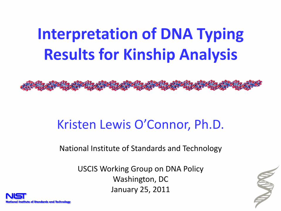
Focusing on 5 markers…Fundamentals of Paternity Testing
Dad
Mom
Child
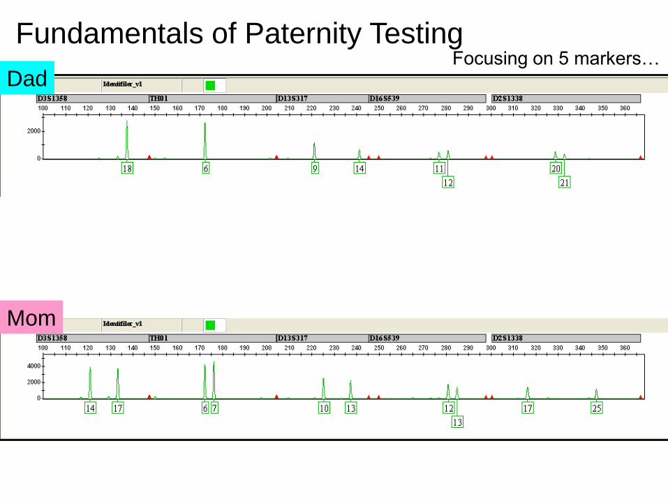
Focus on 5 markers…Fundamentals of Paternity Testing
Parent-offspring will share one allele at every locus
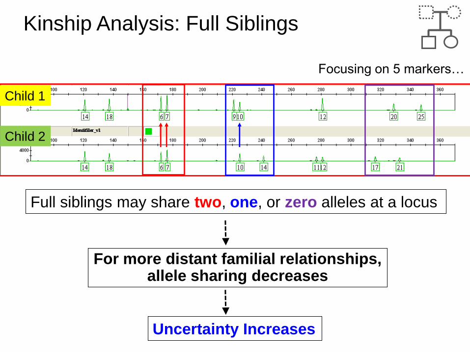
Child 1
Child 2
Full siblings may share two, one, or zero alleles at a locus
Focusing on 5 markers…
Kinship Analysis: Full Siblings
For more distant familial relationships, allele sharing decreases
Uncertainty Increases

Why can kinship analysis be complex?
Relationship 0 alleles 1 allele 2 alleles
Parent-child 0 1 0
Full siblings 1/4 1/2 1/4
Half siblings 1/2 1/2 0
Uncle-nephew 1/2 1/2 0
Grandparent-grandchild 1/2 1/2 0
First cousins 3/4 1/4 0
Half siblings, uncle-nephew, and grandparent-grandchild are genetically identical
Probability of Sharing Alleles from a Common Ancestor
For more distant familial relationships, allele sharing decreases uncertainty increases
Leve
l of
Ce
rtai
nty
High
Low
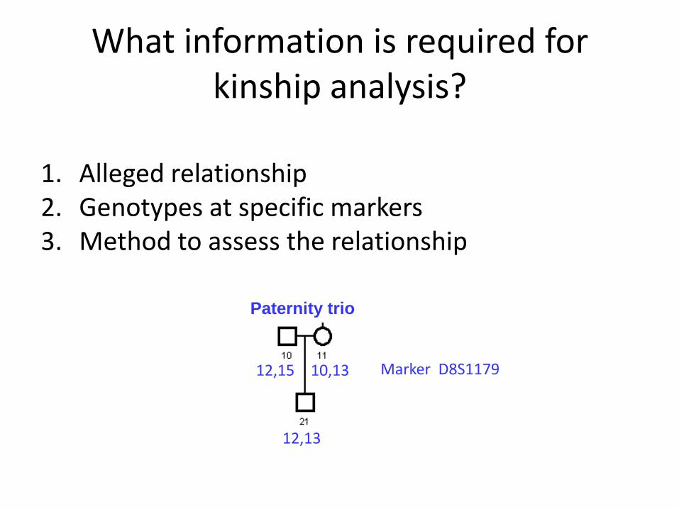
What information is required for kinship analysis?
1. Alleged relationship2. Genotypes at specific markers3. Method to assess the relationship
12,15 10,13
12,13
Paternity trio
Marker D8S1179

What information is required for kinship analysis?
1. Pedigree of claimed relationships
AF M
C
?
Paternity trio
Full siblings
Complex pedigree
Define relationships in a pedigree (“family tree”)
Collect DNA samples from informative individuals

What information is required for kinship analysis?
2. Genotypes for individuals making a claim
Autosomal(passed on in part,
from all ancestors)
• Typically test 13-25 STR loci
• Work well for close relatives
(parentage and full siblings)
• Need more family references
for distant relatives
Y-Chromosome(passed on complete,
but only by sons)
Mitochondrial (passed on complete,
but only by daughters)
Lineage Markers
Butler, J.M. (2005) Forensic DNA Typing, 2nd Edition, Figure 9.1, ©Elsevier Science/Academic Press
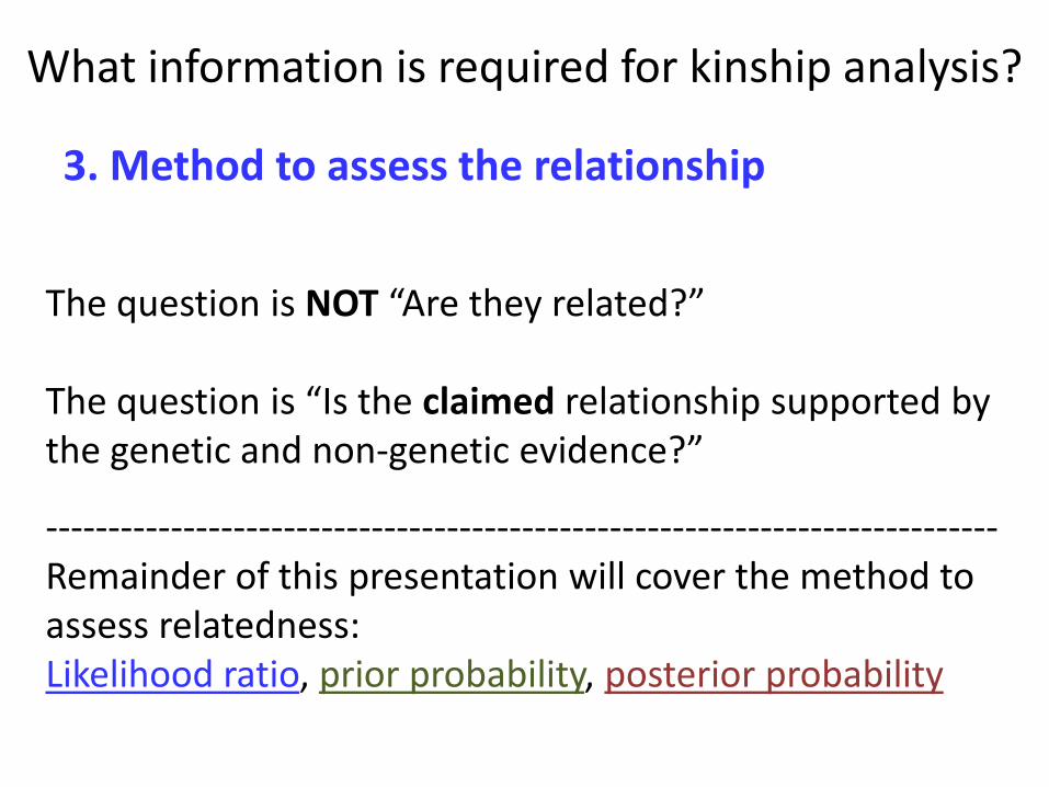
What information is required for kinship analysis?
3. Method to assess the relationship
The question is NOT “Are they related?”
The question is “Is the claimed relationship supported by the genetic and non-genetic evidence?”
----------------------------------------------------------------------------Remainder of this presentation will cover the method to assess relatedness:Likelihood ratio, prior probability, posterior probability

Likelihood Ratio (LR)
Describes how strongly the genotypes support one relationship versus the other relationship
Expresses the likelihood of obtaining the DNA profiles under two mutually exclusive hypotheses
The LR takes into account:• the probability of allele sharing for individuals with a specific
relationship• the allele frequency of alleles• a possible mutation event (if necessary)
Probability of genotypes if individuals are related as claimedProbability of genotypes if individuals are unrelated
LR =

MF
21
Likelihood Ratio (LR)
The LR is also called the relationship index (RI) or kinship index (KI).
Each independent locus tested produces its own relationship index, which can be multiplied by those of other independent loci to calculate a combined relationship index (CRI).
By the definition of a LR:CRI > 1 supports the numerator (claimed relationship)CRI < 1 supports the denominator (alternative relationship)
Larger CRI values provide more support for the claimed relationship
Probability of genotypes if 1,2 are full siblingsProbability of genotypes if 1,2 are unrelated
CRI =

AF M
C
Paternity trio
Likelihood Ratio (LR)Hypothesis 1 = Paternity Trio, Hypothesis 2 = Unrelated
LocusProbability
(Hypothesis 1)Probability
(Hypothesis 2)Likelihood Ratio
D8S1179 0.001545163 0.000574194 2.691012D21S11 0.0003079 0.000171693 1.793322D7S820 0.00078148 0.000138664 5.635774CSF1PO 0.003673636 0.000798261 4.602047D3S1358 0.002522579 0.001086988 2.320706THO1 0.001420379 0.00032926 4.313852D13S317 0.000454644 4.37E-05 10.39317D16S539 9.47E-05 2.80E-05 3.38817D2S1338 4.87E-05 1.15E-05 4.250356D19S433 0.004076747 0.000661891 6.159245VWA 0.000131184 5.26E-05 2.492709TPOX 0.008606737 0.005087928 1.691599D18S51 0.000328927 9.07E-05 3.625514D5S818 0.002742154 0.000772507 3.549682FGA 0.000532767 0.000198233 2.687581
Total 2.27E-47 1.35E-55 168,468,800
LR = 168,468,800
It is 168 million times more likely that we observe these DNA profiles if the Alleged Father is the true father than if an unrelated man is the father of the child.

How do 13 loci perform for kinship analysis?
The degree of overlap corresponds with possible values for false positive or false negative results.
0
0.1
0.2
0.3
0.4
0.5
-10 -8 -6 -4 -2 0 2 4 6 8 10 12 14
RelatedUnrelated
0.668 < -10
median LR=10,000median LR=2.7E-13
Parent-Offspring(1000 simulations)
0
0.1
0.2
0.3
0.4
0.5
-10 -8 -6 -4 -2 0 2 4 6 8 10 12 14
median LR=0.14 median LR=6.9
0
0.1
0.2
0.3
0.4
0.5
-10 -8 -6 -4 -2 0 2 4 6 8 10 12 14
median LR=1.5E-3 median LR=2400
Pro
po
rtio
n o
f si
mu
lati
on
s u
sin
g U
.S. C
auca
sian
alle
le f
req
uen
cies
LR threshold = 1
Full Siblings(5000 simulations)
Half Siblings(1000 simulations)
log10(LR)
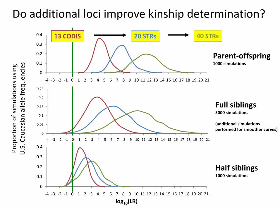
Parent-offspring1000 simulations
Half siblings1000 simulations
Full siblings5000 simulations
(additional simulations performed for smoother curves)
Pro
po
rtio
n o
f si
mu
lati
on
s u
sin
g U
.S. C
auca
sian
alle
le f
req
ue
nci
es
0
0.1
0.2
0.3
0.4
-4 -3 -2 -1 0 1 2 3 4 5 6 7 8 9 10 11 12 13 14 15 16 17 18 19 20 21
0
0.1
0.2
0.3
0.4
-4 -3 -2 -1 0 1 2 3 4 5 6 7 8 9 10 11 12 13 14 15 16 17 18 19 20 21
log10(LR)
20 STRs 40 STRs
0
0.05
0.1
0.15
0.2
0.25
-4 -3 -2 -1 0 1 2 3 4 5 6 7 8 9 10 11 12 13 14 15 16 17 18 19 20 21
13 CODIS
Do additional loci improve kinship determination?

Prior Probability
Describes the weight of non-genetic evidence PRIOR to DNA analysis
Case Prior Probability Comment
Paternity- U.S. courts 0.5 Both hypotheses are equally likely.Different priors could be claimed in court.
Missing Persons (ICMP) 1/N missing persons Closed event (e.g., mass grave)
Immigration- U.S. 0.5 How do you assign weight to non-genetic evidence?
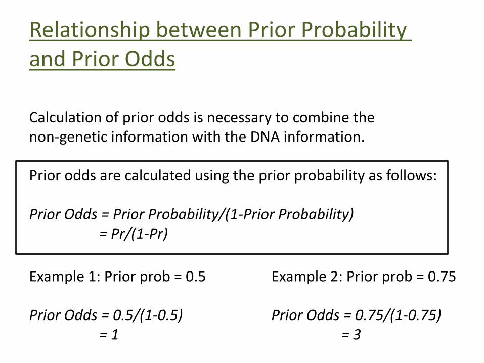
Relationship between Prior Probability and Prior Odds
Calculation of prior odds is necessary to combine the non-genetic information with the DNA information.
Prior odds are calculated using the prior probability as follows:
Prior Odds = Prior Probability/(1-Prior Probability) = Pr/(1-Pr)
Example 1: Prior prob = 0.5 Example 2: Prior prob = 0.75
Prior Odds = 0.5/(1-0.5) Prior Odds = 0.75/(1-0.75) = 1 = 3

Posterior Odds
The posterior odds provide a numerical weight to the opinion of identification.
The mathematics for the combination of the kinship index and the prior odds is as follows:
Posterior Odds = Likelihood Ratio × Prior Odds = CRI × P
Example with prior probability = 0.5 (prior odds = 1), and LR = 168,468,800
Posterior Odds = 168,468,800 × 1= 168,468,800
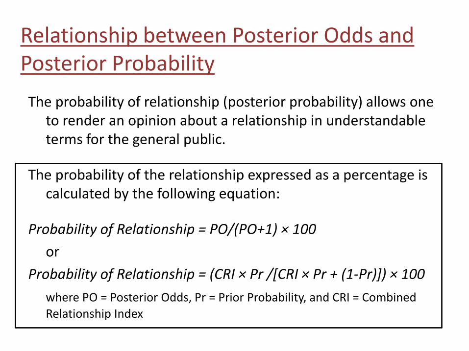
The probability of relationship (posterior probability) allows one to render an opinion about a relationship in understandable terms for the general public.
The probability of the relationship expressed as a percentage is calculated by the following equation:
Probability of Relationship = PO/(PO+1) × 100
or
Probability of Relationship = (CRI × Pr /[CRI × Pr + (1-Pr)]) × 100
where PO = Posterior Odds, Pr = Prior Probability, and CRI = Combined
Relationship Index
Relationship between Posterior Odds and Posterior Probability

Example with prior probability = 0.5 (prior odds = 1), and LR = 168,468,800:
Probability of Relationship = (CRI × Pr /[CRI × Pr + (1-Pr)]) × 100
= (168,468,800 × 0.5 /[168,468,800 × 0.5 + (1-0.5)]) × 100
= 99.999999406418%
Relationship between Posterior Odds and Posterior Probability

Posterior Probability
The probability of relationship (posterior probability) allows one to render an opinion about a relationship in understandable terms for the general public.
Case Posterior Probability Probability of Random Match
Paternity- U.S. courts 99.0-99.9% 0.1-1% (civil cases)
Missing Persons-ICMP 99.95% 0.05%
Immigration 99.5% (currently) 0.5%

Posterior Probability
The probability of relationship (posterior probability) allows one to render an opinion about a relationship in understandable terms for the general public.
Case Posterior Probability Conclusion
Paternity- U.K.(paternity or maternity)
99.99% Positive: Very strong evidence of paternity/maternity
0% Negative: No support for relationship
Sibship- U.K.(full or half sibs)
90.00-99.99% Positive: Very strong evidence of full/half siblingship
10.00-89.99% Inconclusive for relationship
0-9.99% Negative: No support for relationship
Alpha Biolabs
http://www.alphabiolabs.com/assets/files/documents/DOT404VariousTypesofDNATestandtheTestingProcedureIssue01.pdf

Posterior Probability Varies with Different Priors
Table of posterior probabilities for different prior probabilities and likelihood ratios
PriorProbability
Paternity Index (LR)
1 10 100 1,000
0 0 0 0 0
0.001 0.001 0.00991 0.09099 0.5002501
0.010 0.010 0.09174 0.50251 0.9099181
0.100 0.100 0.52631 0.91743 0.9910803
0.500 0.500 0.90909 0.99009 0.9990010
0.900 0.900 0.98901 0.99889 0.9998889
0.990 0.990 0.99899 0.99989 0.9999899
0.999 0.999 0.99989 0.99999 0.9999990
1 1 1 1 1
Evett and Weir, Interpreting DNA Evidence, 1998.

Range of Posterior ProbabilitiesSimulated pairs of individuals, either as true parent-child, full siblings, half siblings, or unrelated. 13 CODIS markers.
Table shows the proportion of simulations within ranges of posterior probabilities (prior probability = 0.5)
Posterior Probability
True Parent-Child
Unrelated Parent-Child
True Full Siblings
Unrelated Full Siblings
True Half Siblings
Unrelated Half Siblings
0-10.0 0 0 0.0076 0.9008 0.017 0.45110.0-20.0 0 0.995 0.0040 0.0356 0.030 0.161
20.0-30.0 0 0.002 0.0060 0.0170 0.034 0.099
30.0-40.0 0 0.002 0.0068 0.0096 0.035 0.074
40.0-50.0 0 0 0.0082 0.0096 0.057 0.06050.0-60.0 0 0.001 0.0088 0.0056 0.055 0.039
60.0-70.0 0 0 0.0086 0.0060 0.077 0.03570.0-80.0 0 0 0.0166 0.0060 0.090 0.027
80.0-90.0 0 0 0.0322 0.0050 0.137 0.02890.0-95.0 0 0 0.0352 0.0020 0.145 0.01795.0-99.0 0.019 0 0.1070 0.0018 0.213 0.009
99.0-99.5 0.024 0 0.0614 0.0006 0.046 099.5-99.9 0.121 0 0.1302 0.0004 0.049 0
99.9-100.0 0.836 0 0.5674 0 0.015 0
Caucasian genotypes simulated with NIST Caucasian allele frequency data. Mutations were not simulated.

Range of Posterior ProbabilitiesSimulated pairs of individuals, either as true parent-child, full siblings, half siblings, or unrelated. 20 markers (CODIS + 7 European markers).
Table shows the proportion of simulations within ranges of posterior probabilities (prior probability = 0.5)
Posterior Probability
True Parent-Child
Unrelated Parent-Child
True Full Siblings
Unrelated Full Siblings
True Half Siblings
Unrelated Half Siblings
0-10.0 0 1.000 0.0022 0.9724 0.012 0.68310.0-20.0 0 0 0.0018 0.0106 0.023 0.097
20.0-30.0 0 0 0.0008 0.0054 0.017 0.053
30.0-40.0 0 0 0.0014 0.0032 0.021 0.039
40.0-50.0 0 0 0.0022 0.0024 0.020 0.04150.0-60.0 0 0 0.0004 0.0012 0.020 0.015
60.0-70.0 0 0 0.0020 0.0012 0.034 0.02370.0-80.0 0 0 0.0026 0.0012 0.049 0.016
80.0-90.0 0 0 0.0092 0.0008 0.084 0.01790.0-95.0 0 0 0.0094 0.001 0.101 0.00895.0-99.0 0 0 0.0266 0.0004 0.198 0.007
99.0-99.5 0 0 0.0120 0 0.106 0.00199.5-99.9 0 0 0.0578 0.0002 0.155 0
99.9-100.0 1.000 0 0.8716 0 0.160 0
Caucasian genotypes simulated with NIST Caucasian allele frequency data. Mutations were not simulated.
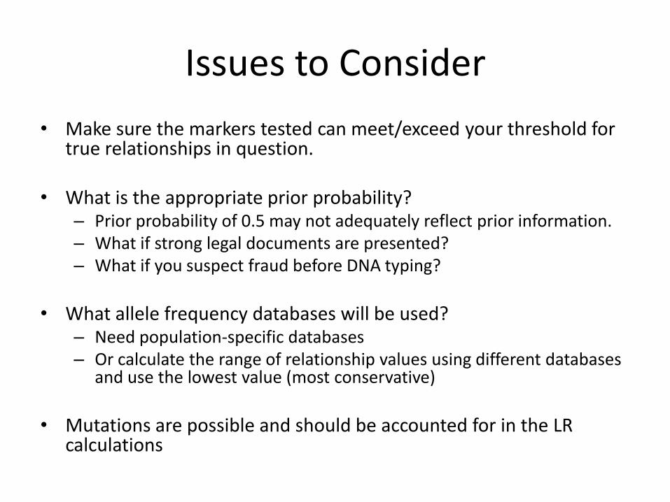
Issues to Consider
• Make sure the markers tested can meet/exceed your threshold for true relationships in question.
• What is the appropriate prior probability? – Prior probability of 0.5 may not adequately reflect prior information.– What if strong legal documents are presented?– What if you suspect fraud before DNA typing?
• What allele frequency databases will be used?– Need population-specific databases– Or calculate the range of relationship values using different databases
and use the lowest value (most conservative)
• Mutations are possible and should be accounted for in the LR calculations
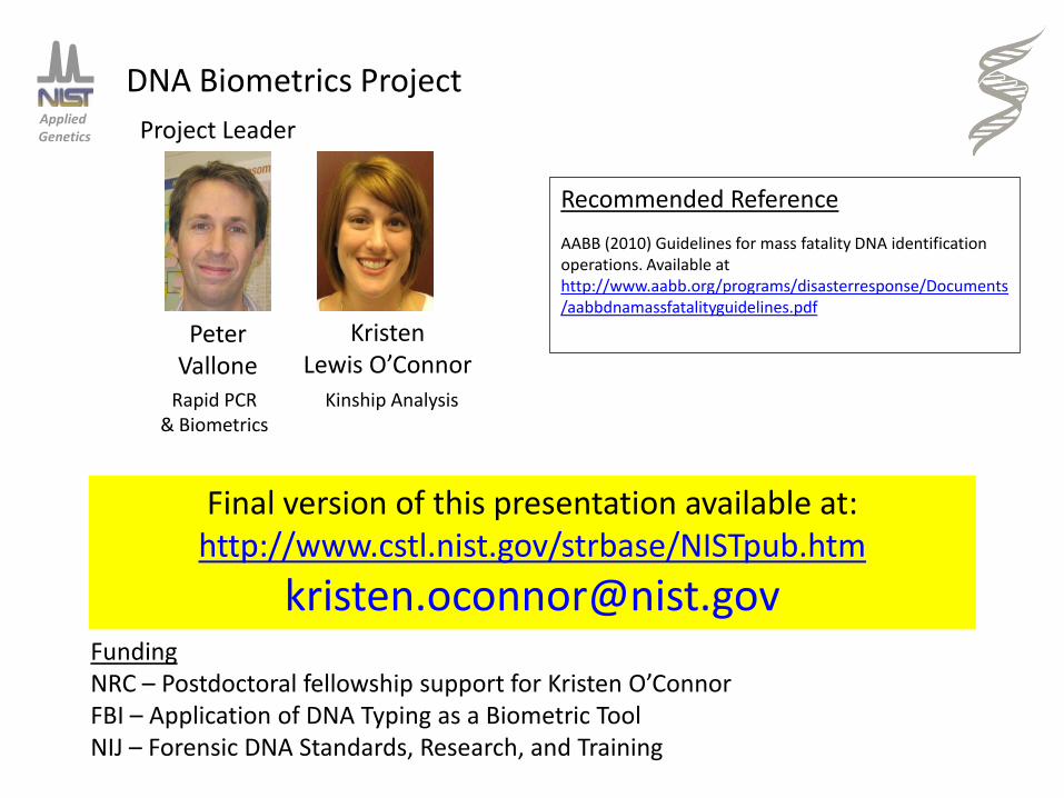
Applied Genetics
Final version of this presentation available at: http://www.cstl.nist.gov/strbase/NISTpub.htm
[email protected] – Postdoctoral fellowship support for Kristen O’ConnorFBI – Application of DNA Typing as a Biometric ToolNIJ – Forensic DNA Standards, Research, and Training
Kristen Lewis O’Connor
Peter Vallone
Project Leader
Rapid PCR & Biometrics
Kinship Analysis
DNA Biometrics Project
Recommended Reference
AABB (2010) Guidelines for mass fatality DNA identification operations. Available at http://www.aabb.org/programs/disasterresponse/Documents/aabbdnamassfatalityguidelines.pdf