Interpretable Biomanufacturing Process Risk and ...
41
RE SEARCH AR TI CLE Interpretable Biomanufacturing Process Risk and Sensitivity Analyses for Quality-by-Design and Stability Control Wei Xie 1 | Bo Wang 1 | Cheng Li 2 | Dongming Xie 3 | Jared Auclair 4 1 Department of Mechanical and Industrial Engineering, Northeastern University, Boston, MA 02115, USA 2 Department of Statistics and Applied Probability, National University of Singapore, Singapore 3 Department of Chemical Engineering, University of Massachusetts Lowell, Lowell, MA 01854, USA 4 Department of Chemistry and Chemical Biology, Northeastern University, Boston, MA 02115, USA Correspondence Wei Xie, Department of Mechanical and Industrial Engineering, Northeastern University, Boston, MA 02115, USA Email: [email protected] While biomanufacturing plays a signicant role in support- ing the economy and ensuring public health, it faces critical challenges, including complexity, high variability, lengthy lead time, and very limited process data, especially for per- sonalized new cell and gene biotherapeutics. Driven by these challenges, we propose an interpretable semantic bio- process probabilistic knowledge graph and develop a game theory based risk and sensitivity analyses for production process to facilitate quality-by-design and stability control. Specically, by exploring the causal relationships and inter- actions of critical process parameters and quality attributes (CPPs/CQAs), we create a Bayesian network based proba- bilistic knowledge graph characterizing the complex causal interdependencies of all factors. Then, we introduce a Shap- ley value based sensitivity analysis, which can correctly quan- tify the variation contribution from each input factor on the outputs (i.e., productivity, product quality). Since the bioprocess model coecients are learned from limited pro- cess observations, we derive the Bayesian posterior distri- bution to quantify model uncertainty and further develop the Shapley value based sensitivity analysis to evaluate the impact of estimation uncertainty from each set of model co- 1 arXiv:1909.04261v4 [stat.ML] 2 Jun 2021
Transcript of Interpretable Biomanufacturing Process Risk and ...
R E S E A RCH ART I C L E
Interpretable Biomanufacturing Process Risk andSensitivity Analyses for Quality-by-Design andStability Control
Wei Xie1 | Bo Wang1 | Cheng Li2 | Dongming Xie3
| Jared Auclair4
1Department of Mechanical and IndustrialEngineering, Northeastern University,Boston, MA 02115, USA2Department of Statistics and AppliedProbability, National University ofSingapore, Singapore3Department of Chemical Engineering,University of Massachusetts Lowell, Lowell,MA 01854, USA4Department of Chemistry and ChemicalBiology, Northeastern University, Boston,MA 02115, USA
CorrespondenceWei Xie, Department of Mechanical andIndustrial Engineering, NortheasternUniversity, Boston, MA 02115, USAEmail: [email protected]
While biomanufacturing plays a significant role in support-ing the economy and ensuring public health, it faces criticalchallenges, including complexity, high variability, lengthylead time, and very limited process data, especially for per-sonalized new cell and gene biotherapeutics. Driven bythese challenges, we propose an interpretable semantic bio-process probabilistic knowledge graph and develop a gametheory based risk and sensitivity analyses for productionprocess to facilitate quality-by-design and stability control.Specifically, by exploring the causal relationships and inter-actions of critical process parameters and quality attributes(CPPs/CQAs), we create a Bayesian network based proba-bilistic knowledge graph characterizing the complex causalinterdependencies of all factors. Then, we introduce a Shap-ley value based sensitivity analysis, which can correctly quan-tify the variation contribution from each input factor onthe outputs (i.e., productivity, product quality). Since thebioprocess model coefficients are learned from limited pro-cess observations, we derive the Bayesian posterior distri-bution to quantify model uncertainty and further developthe Shapley value based sensitivity analysis to evaluate theimpact of estimation uncertainty from each set of model co-
1
arX
iv:1
909.
0426
1v4
[st
at.M
L]
2 J
un 2
021
2 Bioprocess Risk and Sensitivity Analyses
efficients. Therefore, the proposed bioprocess risk and sen-sitivity analyses can identify the bottlenecks, guide the re-liable process specifications and the most informative datacollection, and improve production stability.
K E YWORD S
Bioprocess risk analysis, sensitivity analysis, manufacturingprocess stability control, Bayesian network, process causalinterdependence
1 | INTRODUCTION
Biomanufacturing is growing rapidly and playing an increasingly significant role in supporting the economy and ensur-ing public health. For example, the biopharmaceutical industry generated more than $300 billion in revenue in 2019and more than 40% of the drug products in the development pipeline were biopharmaceuticals (Rader and Langer,2019). However, drug shortages have occurred at unprecedented rates over the past decade. The current systems areunable to rapidly produce new drugs to meet urgent needs in the presence of a major public health emergency. TheCOVID-19 pandemic is having a profound impact globally and caused over 111 millions confirmed cases by February,2021. Even COVID-19 vaccines are discovered, developing the production process and manufacturing the billionsof doses needed to immunize the world’s population will be extremely time-consuming using existing technologies,thus lengthening the time period of human and economic distress. It is critically important to speed up the bioprocessdevelopment and ensure product quality consistency.
However, biomanufacturing faces several critical challenges, including high complexity and variability, and lengthy leadtime (Kaminsky and Wang, 2015). Biomanufacturing is based on living cells whose biological processes are very com-plex and have highly variable outputs. The productivity and product critical quality attributes (CQAs) are determinedby the interactions of hundreds of critical process parameters (CPPs), including raw materials, media compositions,feeding strategy, and process operational conditions, such as pH and dissolved oxygen in the bioreactor. As newbiotherapeutics (e.g., cell and gene therapies) become more and more “personalized", the production, regulation pro-cedure, and analytical testing time required by biopharmaceuticals of complex molecular structure is lengthy, and thehistorical observations are relatively limited in particular for drugs in early stages of production process development.
Therefore, it is crucial to integrate all sources of data and mechanism information, provide the risk- and science-basedunderstanding of the complex bioprocess CPPs/CQAs causal interdependencies, and identify and control the key factorscontributing the most to the output variation. This study can accelerate the development of productive and reliablebiomanufacturing, facilitate building the quality into the production process or quality-by-design (QbD), support real-time monitoring and release, and reduce the time to market.
Various Process Analytical Technologies (PAT) and methodologies have been proposed to improve the bioprocessunderstanding and guide the process development, decision making, and risk control; see the review in Steinwandteret al. (2019). Most PATs are based onmultivariate data analysis; see Section 2. Ordinary or partial differential equations(ODEs/PDEs) based mechanistic models are developed for simulating individual biomanufacturing unit operations;see for example Kyriakopoulos et al. (2018). On the other hand, various operations research/management (OR/OM)methods are also proposed for biomanufacturing system analytics and decision-making; see the review (Kaminsky andWang, 2015). Overall, existing methodologies have the key limitations: (1) the multivariate statistics based PAT and
Bioprocess Risk and Sensitivity Analyses 3
OR/OM approaches focus on developing general methodologies without incorporating the bioprocess causal relation-ship and structural mechanism information, which limits their performance, interpretability, and adoption, especiallywith limited data; and (2) the mechanistic models are usually deterministic and focus on individual unit operationswithout providing an reliable integrated bioprocess learning and risk management framework.
Driven by the critical challenges in the biomanufacturing industry, in this paper, we propose a bioprocess semanticprobabilistic knowledge graph, characterizing the risk- and science-based understanding of integrated productionprocess, which can integrate all sources of heterogeneous data and leverage the information from existing mechanismmodels and historical data. Then, we introduce comprehensive and rigorous bioprocess risk and sensitivity analyses,accounting for model risk, which can guide the process specifications andmost informative data collection to facilitatethe learning and improve the production reliability and stability (e.g., product quality consistency).
The key contributions of this paper are three fold. First, by exploring the causal relationships and interactions ofmany factors within and between operation units (i.e., CPPs/CQAs), such as raw materials, production process param-eters, and product quality, we consider a bioprocess ontology based data integration and develop a Bayesian network(BN) based bioprocess probabilistic knowledge graph, characterizing the process inherent stochastic uncertainty andcausal interdependencies of all input and output factors. Second, building on the process knowledge graph, we in-troduce a game theory – Shapley value (SV) – based sensitivity analysis (SA), considering the complex bioprocessinterdependencies, which can correctly quantify the contribution and criticality of each random input factor on thevariance of outputs (i.e., productivity and product CQAs), identify the bottlenecks, and accelerate the reliable biopro-cess specifications. Third, since the coefficients of interpretable bioprocess model or probabilistic knowledge graphare estimated from limited real-world process data, which induces model uncertainty (MU) or model risk (MR), wefurther propose Bayesian uncertainty quantification and Shapley value based model uncertainty sensitivity analysisto support process learning and faithfully assess the impact of estimation uncertainty from each set of model coeffi-cients. Thus, our study can: (1) identify the bottlenecks of bioprocess; (2) accelerate the reliable process specifications anddevelopment to improve the production process stability and facilitate QbD; and (3) support the most “informative" datacollection to reduce the model risk of process probabilistic knowledge graph and improve the bioprocess understanding.
This paper is organized as follows. In Section 2, we review the related literature on biomanufacturing processmodeling and PATs, Bayesian network, and process sensitivity analysis. In Section 3, we present the problem descrip-tion and summarize the proposed framework. In Section 4, we develop the Bayesian network (BN) based bioprocessprobabilistic knowledge graph to characterize the risk- and science-based process understanding. We derive theShapley value (SV) based bioprocess sensitivity analysis in Section 5 to support the process specifications, improvethe production stability, and ensure product quality consistency. We further introduce the process model coefficientuncertainty quantification and Shapley value based sensitivity analysis studying the impact of each model coefficientestimation uncertainty on process risk analysis and CPPs/CQAs criticality assessment in Section 6. We conduct theempirical study on the performance of our proposed framework in both simulation and real data analysis in Section 7,and then conclude with some discussion in Section 8.
2 | BACKGROUND
The Process Analytical Technologies (PAT) are defined as “a system for designing, analyzing and controlling manufac-turing through timely measurements of critical quality and performance attributes of raw and in-process materials andprocesses, with the goal of ensuring final product quality"; see Pharmaceutical Current GoodManufacturing Practices(CGMPs) (2004). With the established process sensors and analyzers, such as near infrared spectroscopy, Raman
4 Bioprocess Risk and Sensitivity Analyses
spectrocopy, and multiwavelength fluorescence, various multivariate data analysis approaches have been used forbioprocess PATs, including principal component analysis (PCA) (Ayech et al., 2012), partial least squares (PLS) (De Liraet al., 2010), clustering (Prinsloo et al., 2008), multilinear regression (Wechselberger et al., 2012), artificial neural net-work (ANN) (Li and Venkatasubramanian, 2018), genetic algorithm (Sokolov et al., 2018), elastic net (Severson et al.,2015), support vector machines (Li and Yuan, 2006), and root cause analysis (Borchert et al., 2019); see an overviewin Rathore et al. (2010). However, existing PAT approaches are usually based on generalized multivariate “black-box"approaches quantifying the input-output relationship without incorporating the bioprocess mechanism information.
On the other hand, OR/OM methodology development for biomanufacturing analysis and decision making isstill in its infancy (Kaminsky and Wang, 2015). Mixed integer linear programming (Lakhdar et al., 2007; Leachmanet al., 2014), dynamic lot size model (Fleischhacker and Zhao, 2011), and queueing network and simulation models(Lim et al., 2004; Kulkarni, 2015) have been developed to study resource planning, scheduling and material consump-tion in biomanufacturing. Those approaches focus on developing general methodologies without fully exploring thebio-technology domain knowledge (e.g., causal relationship, structural information of the bioprocess). Some recentworks, e.g., Martagan et al. (2016, 2017, 2018), account for physical-chemical characteristics and biology-inducedrandomness in either fermentation or chromatography stage, and develop Markov decision models to optimize thecorresponding operational policies.
For complex systems, Bayesian network (BN) can be used to combine the expert knowledge with data and facil-itate data integration and process analysis in various applications. For example, Wang et al. (2018) proposed a BNbased knowledge management system for additive manufacturing. Troyanskaya et al. (2003) introduced a BN thatcombines evidence from gene co-expression and experimental data to predict whether two genes are functionallyrelated. Moullec et al. (2013) provided a BN approach for system architecture generation and evaluation, and Te-lenko and Seepersad (2014) applied probabilistic graphical model to study how the usage context factors, includinghuman factors, situational factors, and product design factors, impact on the energy consumption of the lightweightvehicle to guide usage scenarios and vehicle designs. Furthermore, Bayesian posterior and belief propagation basedrisk assessment has been studied in information system security (Feng et al., 2014), water mains failure (Kabir et al.,2015), and supply chain (Ojha et al., 2018). Motivated by these studies, we propose a Bayesian network for modelingthe complex interdependence of production process parameters and bio-drug properties, which can fully utilize thestructural knowledge and causal relationship, and integrate the data from end-to-end bioprocess.
Finally, we briefly discuss the related literature on sensitivity analysis; see the review (Borgonovo and Plischke,2016). The existing sensitivity analysis studies associated with Bayesian network tend to systematically vary one ofnetwork’s parameter at a time while fixing the other parameters and then obtain analytic expressions for the sensitiv-ity functions (Van der Gaag et al., 2007; Castillo et al., 1997). In our case, we are interested in stochastic uncertaintycontributed by each factor, which is closely related to global probabilistic sensitivity analysis. Existing literature onglobal sensitivity analysis can be divided into several categories, including: (1) regression based methods, e.g., Helton(1993), which use the standardized regression coefficients as sensitivity measure; (2) variance based methods (Wag-ner, 1995; Sobol, 1993) which assess the contribution of each random input based on expected reduction in modeloutput variance; (3) functional ANOVA decomposition (Rabitz and Aliş, 1999) which provides variance decompositionunder independence through high dimensional model representation theory; (4) density-based methods (Zhai et al.,2014) that directly quantify the output density without reference to a particular moment. Since the commonly usedvariance-based sensitivity measures (i.e., first-order effects and total effects) fail to adequately account for probabilis-tic dependence of inputs and process structural interactions or interdependencies, Owen (2014) introduced a newsensitivity measure based on the game theory, called the Shapley Value (SV). Song et al. (2016) further analyzed thismeasure and proposed a Monte Carlo algorithm for the estimation of Shapley values. Lundberg and Lee (2017) pro-
Bioprocess Risk and Sensitivity Analyses 5
posed Shapley value based unified framework for interpreting predictions. Inspired by these studies, building on theproposed BN-based bioprocess knowledge graph characterizing the process causal interdependencies, we introduceSV-based probabilistic sensitivity analysis to assess the contribution or criticality of each random input (e.g., CPP andCQA ) on the output variance, while accounting for the impact of model estimation uncertainty associated with eachset of model coefficients.
3 | PROBLEM DESCRIPTION AND PROPOSED FRAMEWORK
We create a probabilistic graph model characterizing the risk- and science-based understanding of causal interdependenciesbetween bioprocess CPPs/CQAs, and then propose risk and sensitivity analyses for integrated biomanufacturing process,accounting for model uncertainty. This study can: (1) provide a reliable guidance on process specification, CPPs/CQAsmonitoring, and most informative data collection; (2) facilitate production stability control and quality-by-design(QbD); and (3) accelerate real-time release, speed up the time to market, and reduce the drug shortage.
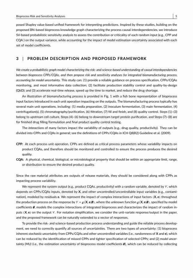
An illustration of biomanufacturing process is provided in Fig. 1 with a fish bone representation of bioprocessinput factors introduced in each unit operation impacting on the outputs. The biomanufacturing process typically hasseveral main unit operations, including: (1) media preparation, (2) inoculum fermentation, (3) main fermentation, (4)centrifugation(s), (5) chromatography/purification, (6) filtration, (7) fill and finish, and (8) quality control. Steps (1)–(3)belong to upstream cell culture, Steps (4)–(6) belong to downstream target protein purification, and Steps (7)–(8) arefor finished drug filling/formulation and final product quality control testing.
The interactions of many factors impact the variability of outputs (e.g., drug quality, productivity). They can bedivided into CPPs and CQAs in general; see the definitions of CPPs/CQAs in ICH Q8(R2) Guideline et al. (2009).
CPP: At each process unit operation, CPPs are defined as critical process parameters whose variability impacts onproduct CQAs, and therefore should be monitored and controlled to ensure the process produces the desiredquality.
CQA: A physical, chemical, biological, or microbiological property that should be within an appropriate limit, range,or distribution to ensure the desired product quality.
Since the raw material attributes are outputs of release materials, they should be considered along with CPPs asimpacting process variability.
We represent the system output (e.g., product CQAs, productivity) with a random variable, denoted byY , whichdepends on CPPs/CQAs inputs, denoted by X, and other uncontrolled/uncontrollable input variables (e.g., contami-nation), modeled by residuals e. We represent the impact of complex interactions of input factors (X, e) throughoutthe production process on the response byY = g (X, e |θθθ) , where the unknown function g (X, e |θθθ) , specified by modelcoefficients θθθ, models the complex interactions of integrated bioprocess and characterizes the impact of random in-puts (X, e) on the output Y . For notation simplification, we consider the unit-variate response/output in the paper,and the proposed framework can be naturally extended to a vector of responses.
To provide the risk- and science-based production process understanding and guide the reliable process develop-ment, we need to correctly quantify all sources of uncertainties. There are two types of uncertainty: (1) bioprocessinherent stochastic uncertainty from CPPs/CQAs and other uncontrolled variables (i.e., randomness of X and e), whichcan be reduced by the identification of missed CPPs and tighter specification of selected CPPs; and (2) model uncer-tainty (MU) (i.e., the estimation uncertainty of bioprocess model coefficients θθθ), which can be reduced by collecting
6 Bioprocess Risk and Sensitivity Analyses
F IGURE 1 An illustration of general biomanufacturing process and fish-bone representation (Walsh, 2013).
“most informative" process observations. Correctly quantifying all sources of uncertainty can facilitate learning, guide riskelimination/control, and improve robust, automatic, and reliable bioprocess decision making.
3.1 | Review of Game Theory based Sensitivity Measure - Shapley Value
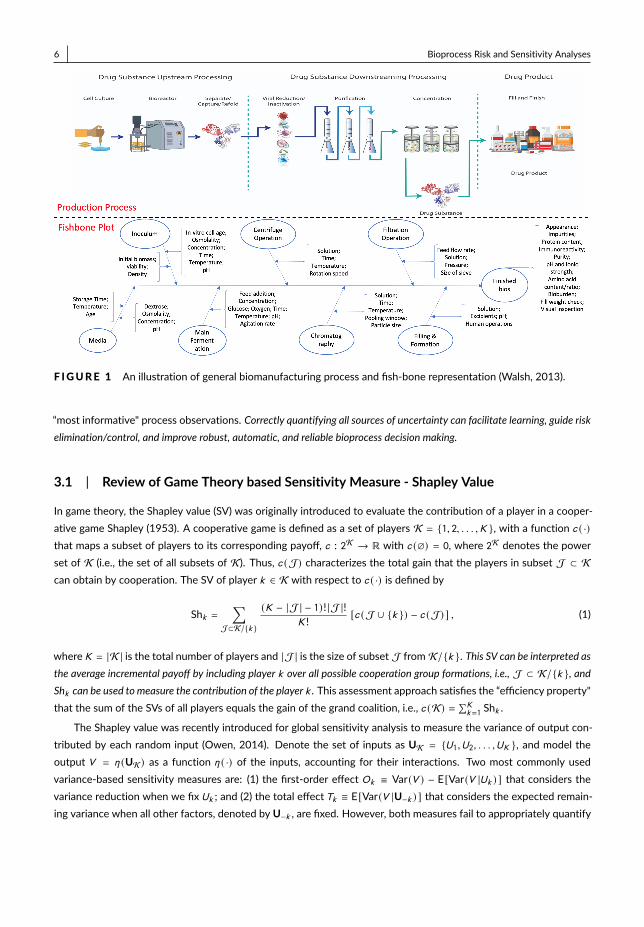
In game theory, the Shapley value (SV) was originally introduced to evaluate the contribution of a player in a cooper-ative game Shapley (1953). A cooperative game is defined as a set of players K = {1, 2, . . . ,K }, with a function c ( ·)that maps a subset of players to its corresponding payoff, c : 2K → Ò with c (∅) = 0, where 2K denotes the powerset of K (i.e., the set of all subsets of K). Thus, c (J) characterizes the total gain that the players in subset J ⊂ Kcan obtain by cooperation. The SV of player k ∈ K with respect to c ( ·) is defined by
Shk =∑
J⊂K/{k }
(K − |J | − 1)! |J |!K ! [c (J ∪ {k }) − c (J) ] , (1)
where K = |K | is the total number of players and |J | is the size of subset J from K/{k }. This SV can be interpreted asthe average incremental payoff by including player k over all possible cooperation group formations, i.e., J ⊂ K/{k }, andShk can be used to measure the contribution of the player k . This assessment approach satisfies the “efficiency property"that the sum of the SVs of all players equals the gain of the grand coalition, i.e., c (K) = ∑K
k=1 Shk .
The Shapley value was recently introduced for global sensitivity analysis to measure the variance of output con-tributed by each random input (Owen, 2014). Denote the set of inputs as UK = {U1,U2, . . . ,UK }, and model theoutput V = η (UK ) as a function η ( ·) of the inputs, accounting for their interactions. Two most commonly usedvariance-based sensitivity measures are: (1) the first-order effect Ok ≡ Var(V ) − E[Var(V |Uk ) ] that considers thevariance reduction when we fix Uk ; and (2) the total effect Tk ≡ E[Var(V |U−k ) ] that considers the expected remain-ing variance when all other factors, denoted by U−k , are fixed. However, both measures fail to appropriately quantify
Bioprocess Risk and Sensitivity Analyses 7
the sensitivity or variance contribution when there exist probabilistic interdependence among inputs and processstructural interaction (Song et al., 2016).
Built on the SV from game theory, given a cooperative game with inputs UK as the players and the payoff as theincremental variance in outputV induced by any index subset J ⊂ K , one can define the payoff function as
c (J) = Var(V ) − E[Var[V |UUUJ ] ] or c (J) = E[Var[V |UUU−J ] ] . (2)
Thus, Owen (2014) introduced a new SV-based sensitivity measure, with ShUk ,V computed by Equations (1) and (2).In this paper, we use c (J) = E[Var[V |UUU−J ] ] in Equation (1), which can simplify the computation of the contributionfrom any random inputUk on the output variance Var(V ) , ShUk ,V = Shk . The SV-based sensitivity analysis overcomesthe limitations of first-order effect and total effect measures by accounting for the interdependence of inputs andprocess interactions. The variance of outputV can be decomposed into the contribution from each random inputUkand we can define the criticality as the proportion of Var(V ) contributed from Uk , denoted by pUk ,V ,
Var(V ) =K∑k=1
ShUk ,V and pUk ,V =ShUk ,VVar(V ) .
The main benefits of SV over first-order and total effect sensitivity measures include: (1) the uncertainty contri-butions sum up to total variance of output; and (2) SV can automatically account for probabilistic dependence andstructural interactions occurring in the complex production process.
3.2 | Summary of Proposed Interpretable Bioprocess Model, Risk and SensitivityAnalyses for Integrated Bioprocess Stability Control
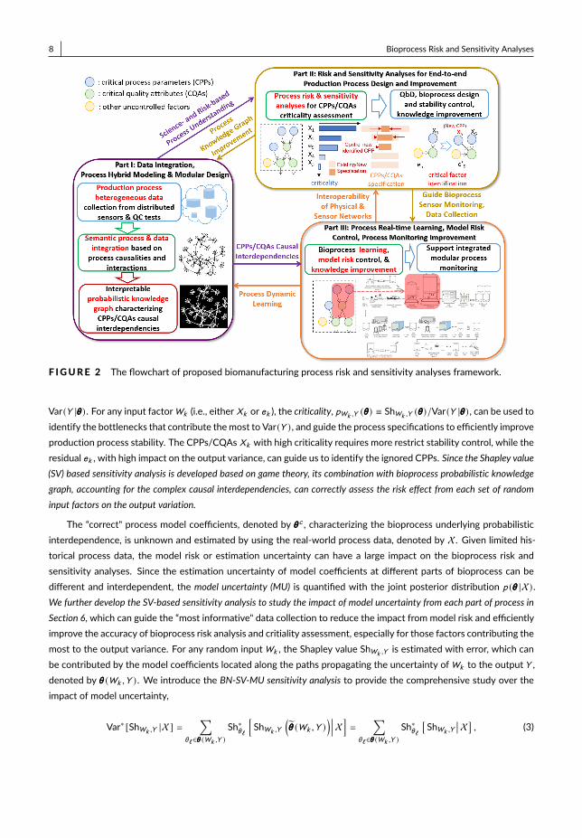
Fig. 2 provides the flowchart of proposed risk and sensitivity analyses framework, which can accelerate learning ofthe end-to-end production process and guide the development of stable biomanufacturing. Parts I and II focus onmodeling and reducing of process stochastic uncertainty. Part III focuses on analyzing and controlling the model risk.By exploring the causal relationships and interactions of CPPs/CQAs of raw materials/in-process materials/productwithin and between different process modules, in Section 4, we develop ontology based data integration and createan interpretable Bayesian network (BN) based bioprocess semantic probabilistic knowledge graph, specified by themodel coefficients θθθ. This knowledge graph can characterize the risk- and science-based understanding of integratedbioprocess and quantify the causal interdependencies of inputs (X, e) and output Y . It is interpretable and extendable,which can support flexible process modular design, incorporate the existing mechanisms from different modules and oper-ation units, quantify the bioprocess causal interdependencies, and greatly reduce the dimensionality of bioprocess designspace to guide the decision making.
Building on this interpretable probabilistic knowledge graph, in Section 5, we develop the SV-based process riskand sensitivity analyses studying stochastic uncertainty, and derive variance decomposition to quantify the contribu-tion from each random input,
Var(Y |θθθ) =∑Xk
ShXk ,Y (θθθ) +∑ek
Shek ,Y (θθθ),
where Shapley values, ShXk ,Y (θθθ) and Shek ,Y (θθθ) , measure the contributions from any CPP/CQA, Xk ∈ X, and residualfactor, ek ∈ e (representing the impact of remaining uncontrolled factors on the CQA Xk ), to the output variance
8 Bioprocess Risk and Sensitivity Analyses
F IGURE 2 The flowchart of proposed biomanufacturing process risk and sensitivity analyses framework.
Var(Y |θθθ) . For any input factorWk (i.e., either Xk or ek ), the criticality, pWk ,Y (θθθ) ≡ ShWk ,Y (θθθ)/Var(Y |θθθ) , can be used toidentify the bottlenecks that contribute themost to Var(Y ) , and guide the process specifications to efficiently improveproduction process stability. The CPPs/CQAs Xk with high criticality requires more restrict stability control, while theresidual ek , with high impact on the output variance, can guide us to identify the ignored CPPs. Since the Shapley value(SV) based sensitivity analysis is developed based on game theory, its combination with bioprocess probabilistic knowledgegraph, accounting for the complex causal interdependencies, can correctly assess the risk effect from each set of randominput factors on the output variation.
The “correct" process model coefficients, denoted by θθθc , characterizing the bioprocess underlying probabilisticinterdependence, is unknown and estimated by using the real-world process data, denoted by X. Given limited his-torical process data, the model risk or estimation uncertainty can have a large impact on the bioprocess risk andsensitivity analyses. Since the estimation uncertainty of model coefficients at different parts of bioprocess can bedifferent and interdependent, the model uncertainty (MU) is quantified with the joint posterior distribution p (θθθ |X) .We further develop the SV-based sensitivity analysis to study the impact of model uncertainty from each part of process inSection 6, which can guide the “most informative" data collection to reduce the impact from model risk and efficientlyimprove the accuracy of bioprocess risk analysis and critiality assessment, especially for those factors contributing themost to the output variance. For any random inputWk , the Shapley value ShWk ,Y is estimated with error, which canbe contributed by the model coefficients located along the paths propagating the uncertainty ofWk to the outputY ,denoted by θθθ (Wk ,Y ) . We introduce the BN-SV-MU sensitivity analysis to provide the comprehensive study over theimpact of model uncertainty,
Var∗ [ShWk ,Y |X] =∑
θ` ∈θθθ (Wk ,Y )Sh∗θ`
[ShWk ,Y
(θθθ (Wk ,Y )
)��� X]=
∑θ` ∈θθθ (Wk ,Y )
Sh∗θ`[ShWk ,Y
�� X], (3)
Bioprocess Risk and Sensitivity Analyses 9
where the subscript “∗" represents any measure calculated based on the posterior p (θθθ |X) and Sh∗θ` [ · | X] measuresthe contribution from coefficient estimation uncertainty of θ` ∈ θθθ (Wk ,Y ) . In the proposed interpretable bioprocessmodel, θ` can be interpreted as certain mechanistic coefficients (e.g., cell growth rate in the cell culture). Thus, thedecomposition in (3) provides the detailed information on how the model uncertainty of each part of integrated pro-duction process influences the estimation uncertainty of ShWk ,Y .
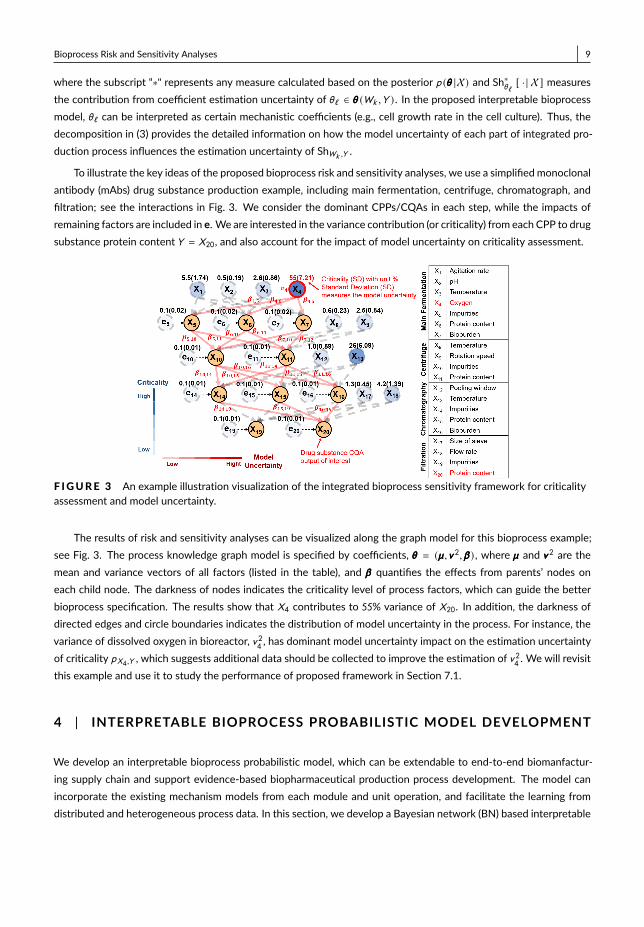
To illustrate the key ideas of the proposed bioprocess risk and sensitivity analyses, we use a simplified monoclonalantibody (mAbs) drug substance production example, including main fermentation, centrifuge, chromatograph, andfiltration; see the interactions in Fig. 3. We consider the dominant CPPs/CQAs in each step, while the impacts ofremaining factors are included in e. We are interested in the variance contribution (or criticality) from each CPP to drugsubstance protein contentY = X20, and also account for the impact of model uncertainty on criticality assessment.
F IGURE 3 An example illustration visualization of the integrated bioprocess sensitivity framework for criticalityassessment and model uncertainty.
The results of risk and sensitivity analyses can be visualized along the graph model for this bioprocess example;see Fig. 3. The process knowledge graph model is specified by coefficients, θθθ = (µµµ,vvv 2,βββ ) , where µµµ and vvv 2 are themean and variance vectors of all factors (listed in the table), and βββ quantifies the effects from parents’ nodes oneach child node. The darkness of nodes indicates the criticality level of process factors, which can guide the betterbioprocess specification. The results show that X4 contributes to 55% variance of X20. In addition, the darkness ofdirected edges and circle boundaries indicates the distribution of model uncertainty in the process. For instance, thevariance of dissolved oxygen in bioreactor, v 24 , has dominant model uncertainty impact on the estimation uncertaintyof criticality pX4,Y , which suggests additional data should be collected to improve the estimation of v 24 . We will revisitthis example and use it to study the performance of proposed framework in Section 7.1.
4 | INTERPRETABLE BIOPROCESS PROBABILISTIC MODEL DEVELOPMENT
We develop an interpretable bioprocess probabilistic model, which can be extendable to end-to-end biomanfactur-ing supply chain and support evidence-based biopharmaceutical production process development. The model canincorporate the existing mechanism models from each module and unit operation, and facilitate the learning fromdistributed and heterogeneous process data. In this section, we develop a Bayesian network (BN) based interpretable
10 Bioprocess Risk and Sensitivity Analyses
bioprocess probabistic knowledge graph, which can characterize the complex CPPs/CQAs causal interdependenciesand support flexible modular biomanfuacturing development.
By exploring the causal relationships and interactions, we consider bioprocess ontology-based data integration,which can connect all distributed and heterogeneous data collected from bioprocess; see more description in OnlineAppendix A. This relational graph can enable the connectivity of end-to-end process. Nodes represent factors (i.e.,CPPs/CQAs, media feed, bioreactor operating conditions, other uncontrolled factors) impacting the process outputs,and the directed edges model the causal relationships. Within each module, which can be each phase of cell cul-ture process (such as cell growth and production phases) or each unit operation, we can model complex interactions,e.g., biological/physical/chemical interactions. In the relational graph, the shaded nodes represent the variables withreal-world observations, including the testing and sensor monitoring data of CPPs/CQAs for raw materials, opera-tion conditions, and intermediate/final drug products. The unshaded nodes represent variables without observationsand residuals, including quality status of intermediate and final drug products, and other uncontrollable factors (e.g.,contamination) introduced during the process unit operations. Since bio-products have very complex structures, wecannot observe the underlying complete quality status and themonitoring of CQAs can carry partial information. Build-ing on the bioprocess relational graph, we develop a BN based probabilistic graphical model composing of randomCPPs/CQAs/residuals factors and their conditional dependencies via directed edges. It can characterize the probabilis-tic causal interdependencies among all factors of integrated bioprocess.
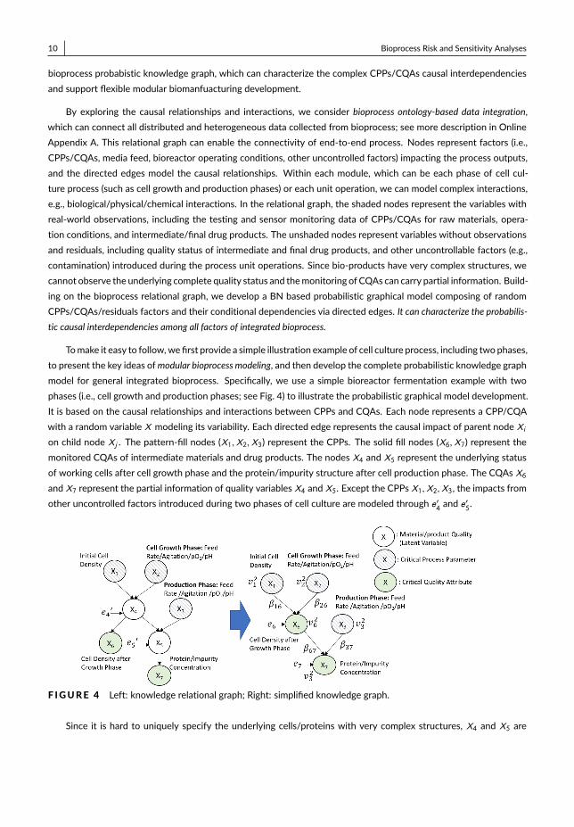
Tomake it easy to follow, we first provide a simple illustration example of cell culture process, including twophases,to present the key ideas ofmodular bioprocess modeling, and then develop the complete probabilistic knowledge graphmodel for general integrated bioprocess. Specifically, we use a simple bioreactor fermentation example with twophases (i.e., cell growth and production phases; see Fig. 4) to illustrate the probabilistic graphical model development.It is based on the causal relationships and interactions between CPPs and CQAs. Each node represents a CPP/CQAwith a random variable X modeling its variability. Each directed edge represents the causal impact of parent node Xion child node Xj . The pattern-fill nodes (X1,X2,X3) represent the CPPs. The solid fill nodes (X6,X7) represent themonitored CQAs of intermediate materials and drug products. The nodes X4 and X5 represent the underlying statusof working cells after cell growth phase and the protein/impurity structure after cell production phase. The CQAs X6and X7 represent the partial information of quality variables X4 and X5. Except the CPPs X1,X2,X3, the impacts fromother uncontrolled factors introduced during two phases of cell culture are modeled through e′4 and e
′5.
F IGURE 4 Left: knowledge relational graph; Right: simplified knowledge graph.
Since it is hard to uniquely specify the underlying cells/proteins with very complex structures, X4 and X5 are
Bioprocess Risk and Sensitivity Analyses 11
hidden, which can lead to an identification issue. Typically, the non-identifiable BN with hidden nodes is transformedto the equivalent BN by structural simplification to avoid analytical issues (see Chapter 19 in Koller and Friedman(2009)). Thus, we simplify and transform the relational graphical model to a graph without hidden nodes, depictedin the right panel of Fig. 4. The new residual e6 in updated graph accounts for both original residual e′4 and also theuncertainty of underlying cell health status, X4, impacting on CQA X6, similar for new residual e7. According to theright plot in Fig. 4, the sources of bioprocess stochastic uncertainty impacting on the variability of X7 include CPPs,(X1,X2,X3) , and other factors with the impact represented by residuals (e6, e7) . Thus, we have CPPs X1,X2 as inputsand CQA X6 as output for the first cell growth phase, and have CQA X6 and CPP X3 as inputs and X7 as output forthe second protein production phase. To study the impact of each CPP on the CQA of interest (i.e., X6 and X7), wecan decompose the variance of X6 and X7 into the contributions from X1, X2 and X3, and remaining parts comingfrom e6 and e7; see the process risk and sensitivity analyses in Section 5. In this way, we can identify the main sourcesof uncertainty and quantify their impacts, which can guide the CPPs/CQAs specifications and the quality control toimprove the product quality stability.
Now we describe the BN-based bioprocess model for general situations. Suppose that the integrated bioprocesscan be represented by a probabilistic graphical model with m +1 nodes: m process factors (denoted by X) and a singleresponse, denoted by Y , such as the impurity concentration or protein content. Let the first mp nodes representingCPPs Xp = {X1,X2, . . . ,Xmp }, the nextma nodes representing CQAs Xa = {Xmp+1,Xmp+2, . . . ,Xm }, and the last noderepresenting the responseY , Xm+1 with m = mp + ma . The modular bioprocess probabilistic knowledge graph can bemodeled by marginal and conditional distributions of each node as follows:
Xk ∼ N(µk ,v 2k ) for CPP Xk with k = 1, 2, . . . ,mp , (4)
Xk = f (P a (Xk ) ;θθθk ) + ek for CQA Xk with k = mp + 1, . . . ,m + 1 (5)
whereN(u,v 2) denotes the normal distributionwithmean u and variance v 2, and P a (Xk ) denotes the parent nodes ofXk . By applying central limit theory (CLT), we assume that the residual ek ∼ N(0,v 2k ) with the conditional variancev
2k≡
Var[Xk |P a (Xk ) ]. Since the amount of real-world bioprocess batch data is often very limited, Gaussian distribution isused to model the variability of each variable or node, which is often used in the existing biopharmaceutical studies(see for example Coleman and Block (2006)). It also makes the process risk and sensitivity analyses tractable.
The proposed probabilistic knowledge graph is a hybrid model of integrated bioprocess, which can leverage the existingmechanisms and learn from real-world process data. Basically, the prior of the function f ( ·) in a generalized regressionmodel (5) can be specified based on the existing knowledge on underlying bioprocess mechanisms (e.g., biophysic-ochemical kinetics) within each module of bioprocess; see for example Kyriakopoulos et al. (2018); Lu et al. (2018);Doran (1995). The unknown model coefficients θθθk (e.g., cell growth rate, media consumption rate) need be estimatedfrom process data. In this paper, we consider linear function accounting for the main effects, i.e.,
Xk = µk +∑
Xj ∈P a (Xk )βj k (Xj − µj ) + ek for CQA Xk with k = mp + 1, . . . ,m + 1 (6)
where the coefficient βj k can be used to measure the effect from the parent node Xj to child node Xk .
Here, we use some illustrative examples to briefly show how the proposed Bayesian network based processprobabilisticmodel allows us to incorporate the existing bioprocessmechanisms. We first consider the cell exponentialgrowth mechanism for the fermentation step, x = x0eµt , where x0 and x denote the starting and ending cell densities,and µ is the unknown growth rate. This is a commonly used mechanismmodel in biomanufacturing industry; see more
12 Bioprocess Risk and Sensitivity Analyses
information in Doran (2013). Suppose that there is a fixed cell culture duration t . By doing the log transformation andsetting Xk = log(x0) , Xk+1 = log(x ) and β0 = µt , we can take the exponential growth mechanism as prior and get thehybrid probabilistic model for the exponential growth phase in fermentation or cell culture process,Xk+1 = β0+Xk +ek ,where ek represents the residual term characterizing the integrated effect from many other factors and it follows aGaussian distribution by following CLT. Notice that it is a special case of BN-based process model (6). The similar ideacan be applied to the situations where we have PDE/ODE-based bioprocess kinetics mechanism models,
d
d tx (t ) = f (x (t ) ; θt ) ≈
x (tk+1) − x (tk )tk+1 − tk
= f (x (tk ) ; θtk ),
where x (t ) can represent the concentrations of protein and metabolite waste at time t and θt can denote the nonsta-tionary growth rate. We can take the existing mechanism model as the prior knowledge of production process. Byapplying the finite difference on the gradient dx (t )/d t and first-order Taylor approximation on function f ( ·) , we canconstruct a probabilistic hybrid model matching with the formula in Equation (6), which can leverage the informationfrom existing PDE/ODE-based bioprocess kinetics mechanism models. This approximation can be very accurate ifthe data are collected from real-time production process sensor monitoring with high sampling frequency.
The complex bioprocess CPPs/CQAs causal interdependencies are characterized by the BN-based probabilisticknowledge graph. Given the model parameters θθθ = (µµµ,vvv 2,βββ ) with mean µµµ = (µ1, . . . , µm+1)>, conditional variancevvv 2 = (v 21 , . . . ,v
2m+1)
>, and linear coefficients βββ = {βj k ; k = mp + 1, . . . ,m + 1 and Xj ∈ P a (Xk ) }, the conditionaldistribution for each CQA node Xk becomes,
p (Xk |P a (Xk )) = N©«µk +
∑Xj ∈P a (Xk )
βj k (Xj − µj ),v 2kª®¬ for k = mp + 1 . . . ,m + 1.
For any CPP node Xk without parent nodes, P a (Xk ) is an empty set and P (Xk |P a (Xk )) is just the marginal distribu-tion P (Xk ) in (4). Therefore, the joint distribution characterizing the interdependencies of CPPs and CQAs involved in theproduction process can be written as p (X1,X2, . . . ,Xm+1) =
∏m+1k=1 p (Xk |P a (Xk )) .
5 | PROCESS RISK AND SENSITIVITY ANALYSES
Given the bioprocess probabilistic knowledge graph specified by the coefficients θθθ = (µµµ,vvv 2,βββ ) , we develop the BN-SVbased sensitivity analysis for integrated production process and quantify the criticality of each random input factormeasuringits contribution to the output variance Var(Xm+1) . This study can guide the CPPs/CQAs specification and improve theproduction process stability. To make it easy to follow, we start with a simple illustration example, provide the generalprocess risk and sensitivity analyses, and then present the algorithm at the end of this section.
We again use the simple example in Fig. 4 to illustrate the results of proposed BN-SV based bioprocess risk andsensitivity analyses, which can decompose the output variance of protein/impurity concentration X7 after fermenta-tion process to each random input – including X1, X2, X3, e6, e7 – as
V ar (X7 |θθθ) = (β16β67)2v 21︸ ︷︷ ︸contribution from X1
+ (β26β67)2v 22︸ ︷︷ ︸contribution from X2
+ β 237v23︸︷︷︸
contribution from X3
+ β 267v26︸︷︷︸
contribution from e6
+ v 27︸︷︷︸contribution from e7
. (7)
The variance contribution from each random input, denoted byWk (i.e., X1,X2,X3, e6, e7), depends on its variance v 2k

Bioprocess Risk and Sensitivity Analyses 13
and the product of coefficients βββ located along the paths propagating the uncertainty fromWk to the output X7; seeFig. 5. The darker blue filled node (i.e., cell growth phase CPP X2, feed rate) contributes more to the output varianceand has higher criticality. Thus, to efficiently reduce the output variance, it requires more restrictive stability control.The high impact of e7 (with darker color) can guide us to identify unrecognized or missed CPPs.
F IGURE 5 A simple example to illustrate BN-SV based process risk and sensitivity analysis.
This simple example illustrates that the proposed production process BN-SV risk and sensitivity analyses andthe CPPs/CQAs criticality assessment are based on the bioprocess probabilistic knowledge graph, characterizing thecomplex CPPs/CQAs causal interdependencies and accounting for all sources of process inherent uncertainty, whichcan (1) guide the process specifications; (2) improve the product quality consistency and bioprocess stability; and (3)advance the risk- and science-based understanding on bioprocess.
Now we present the general process risk and sensitivity analyses. We first derive the Shapley value (SV) quanti-fying the contribution of each random input factor from CPPs Xp and other factors e to Var(Xm+1) , which accountsfor cases with dependent input factors. According to the Gaussian BN model presented in (4) and (6), we can write
Xm+1 = µm+1 +mp∑k=1
γk ,m+1 (Xk − µk ) +m+1∑
k=mp+1
γk ,m+1ek , (8)
where the weight coefficient of any CPP Xk to CQA Xn with k ≤ mp < n ≤ m + 1,
γk n = βk n +∑
mp<`<n
βk `β`n +∑
mp<`1<`2<n
βk `1β`1`2β`2n + . . . + βk ,mp+1βmp+1,mp+2 . . . βn−1,n , (9)
the weight coefficient of any ek to a CQA node Xn with mp < k < n ≤ m + 1,
γk n = βk n +∑k<`<n
βk `β`n +∑
k<`1<`2<n
βk `1β`1`2β`2n + . . . + βk ,k+1βk+1,k+2 . . . βn−1,n ; (10)
and γnn = 1 for any n; see the derivation for (8) in Appendix B. The weight coefficient γk n is the product sum of βββlocated along the paths from node Xk to node Xn in the graph model. LetWWW = {X1, . . . ,Xmp , emp+1, . . . , em+1 } ,{W1,W2, . . . ,Wm+1 } represent all random input factors, with the index set K = {1, 2, . . . ,m + 1}. Then, the SV for thek -th factorWk is,
ShWk ,Xm+1 =∑
J⊂K/{k }
(m − |J |)! |J |!(m + 1)! [c (J ∪ {k }) − c (J) ] .
14 Bioprocess Risk and Sensitivity Analyses
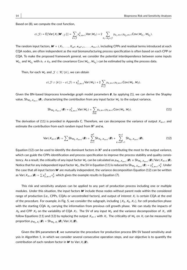
Based on (8), we compute the cost function,
c (J) = E[Var[Xi |WWW −J ] ] =∑k ∈J
γ2k ,m+1Var(Wk ) + 2∑
k1<k2∈Jγk1,m+1γk2,m+1Cov(Wk1 ,Wk2 ) .
The random input factors,WWW = (X1, . . . ,Xmp , emp+1, . . . , em+1) , including CPPs and residual terms introduced at eachCQA nodes, are often independent as the real biomanufacturing process specification is often based on each CPP orCQA. To make the proposed framework general, we consider the potential interdependence between some inputsWk1 andWk2 with k1 , k2, and the covariance Cov(Wk1 ,Wk2 ) can be estimated by using the process data.
Then, for eachWk and J ⊂ K/{k }, we can obtain
c (J ∪ {k }) − c (J) = γ2k ,m+1Var(Wk ) + 2∑`∈J
γk ,m+1γ` ,m+1Cov(Wk ,W` ) .
Given the BN-based bioprocess knowledge graph model parameters θθθ, by applying (1), we can derive the Shapleyvalue, ShWk ,Xm+1 (θθθ) , characterizing the contribution from any input factorWk to the output variance,
ShWk ,Xm+1 (θθθ) = γ2k ,m+1Var(Wk ) +
∑`,k
γk ,m+1γ` ,m+1Cov(Wk ,W` ) . (11)
The derivation of (11) is provided in Appendix C. Therefore, we can decompose the variance of output Xm+1 andestimate the contribution from each random input from Xp and e,
Var(Xm+1 |θθθ) =∑
ShWk ,Xm+1 (θθθ) =mp∑k=1
ShXk ,Xm+1 (θθθ) +m+1∑
k=mp+1
Shek ,Xm+1 (θθθ) . (12)
Equation (12) can be used to identify the dominant factors in Xp and e contributing the most to the output variance,which can guide the CPPs identification and process specification to improve the process stability and quality consis-tency. As a result, the criticality of any input factorWk can be calculated as pWk ,Xm+1 (θθθ) ≡ ShWk ,Xm+1 (θθθ)/Var(Xm+1 |θθθ) .Notice that for any independent input factorWk , the SV in Equation (11) is reduced to ShWk ,Xm+1 (θθθ) = γ
2k ,m+1v
2k. Under
the case that all input factorsWWW are mutually independent, the variance decomposition Equation (12) can be writtenas Var(Xm+1 |θθθ) =
∑γ2k ,m+1v
2k, which gives the example results in Equation (7).
This risk and sensitivity analyses can be applied to any part of production process including one or multiplemodules. Under this situation, the input factorsWWW include those nodes without parent node within the consideredrange of production (i.e., CPPs, CQAs or uncontrolled factors), and output of interest Xi is certain CQA at the endof the procedure. For example, in Fig. 5, we consider the subgraph, including {X3,X6,X7 }, for cell production phasewith the starting CQA X6 carrying the information from previous cell growth phase. We can study the impacts ofX6 and CPP X3 on the variability of CQA X7. The SV of any inputWk and the variance decomposition of Xi , stillfollow Equations (11) and (12) by replacing the output Xm+1 with Xi . The criticality ofWk on Xi can be measured byproportion pWk ,Xi (θθθ) = ShWk ,Xi (θθθ)/Var(Xi |θθθ) .
Given the BN parameters θθθ, we summarize the procedure for production process BN-SV based sensitivity anal-ysis in Algorithm 1, in which we consider several consecutive operation steps, and our objective is to quantify thecontribution of each random factor inWWW to Var(Xi |θθθ) .

Bioprocess Risk and Sensitivity Analyses 15
Algorithm 1: Procedure for Production Process BN-SV based Sensitivity AnalysisInput: BN parameters θθθ, group of input factorsWWW , response node Xm+1.Output: Variance decomposition of Xi in terms of all random inputs withinWWW .(1) Calculate the Shapley value ShWk ,Xm+1 (θθθ) by using Equation (11), which measures the contribution fromWk to thevariance of response CQA Xm+1;
(2) Provide the variance decomposition of Var(Xm+1 |θθθ) by using Equation (12), and obtain the criticality ofWk on thevariance of Xm+1: pWk ,Xm+1 (θθθ) = ShWk ,Xm+1 (θθθ)/Var(Xm+1 |θθθ) .
6 | SENSITIVITY ANALYSIS FOR MODEL RISK REDUCTION
Since the underlying true process model coefficients θθθc are unknown, given finite real-world data X, there exists themodel uncertainty (MU) characterizing our limited knowledge on the probabilistic interdependence of integrated bio-process. To study the impact of MU on the production process risk and sensitivity analyses for stochastic uncertaintyand further assess CPPs/CQAs criticality, we propose the BN-SV-MU based uncertainty quantification and sensitivityanalysis, which can guide the process monitoring and “most informative" data collection. In Section 6.1, we developthe posterior p (θθθ |X) and a Gibbs sampler to generate posterior samples, θθθ (b ) ∼ p (θθθ |X) with b = 1, 2, . . . ,B , quantify-ing the model uncertainty, and then we quantify the overall impact of model uncertainty on the process risk analysisand CPPs/CQAs criticality assessment. In Section 6.2, we propose the BN-SV-MU based sensitivity analysis, whichcan study the impact of each model coefficient(s) estimation uncertainty on the process risk analysis and criticalityassessment; see the result visualization in Fig. 3.
6.1 | Bayesian Learning and Model Uncertainty Quantification
We consider the case with R batches of complete production process data, denoted as X = {(x (r )1 , x(r )2 , . . . , x
(r )m+1), r =
1, 2, . . . , R }. Without strong prior information, we consider the following conjugate (vague) prior (with initial hyperpa-rameters giving relatively flat density),
p (µµµ,vvv 2,βββ ) =m+1∏i=1
p (µi )p (v 2i ) ·∏i,j
p (βi j ), (13)
with p (µi ) = N(µ (0)i ,σ(0)2i), p (v 2
i) = Inv-Γ
(κ(0)i
2,λ(0)i
2
)and p (βi j ) = N(θ (0)i j , τ
(0)2i j) , where Inv-Γ denotes the inverse-
gamma distribution. Given the data X, by applying the Bayes’ rule, we can obtain the posterior distribution
p (µµµ,vvv 2,βββ |X) ∝R∏r=1
[m+1∏i=1
p (x (r )i|x (r )P a (Xi )
)]p (µµµ,vvv 2,βββ ), (14)
quantifying the model uncertainty.
Then, we develop a Gibbs sampler to generate the posterior samples from (14) quantifying the model uncertainty.We derive the conditional posterior for each parameter in (µµµ,vvv 2,βββ ) . Let µµµ−i , vvv 2−i and βββ−i j denote the collection ofparameters µµµ,vvv 2,βββ excluding the i -th or (i , j )-th element. Let S (Xi ) denote the set of direct succeeding or child
16 Bioprocess Risk and Sensitivity Analyses
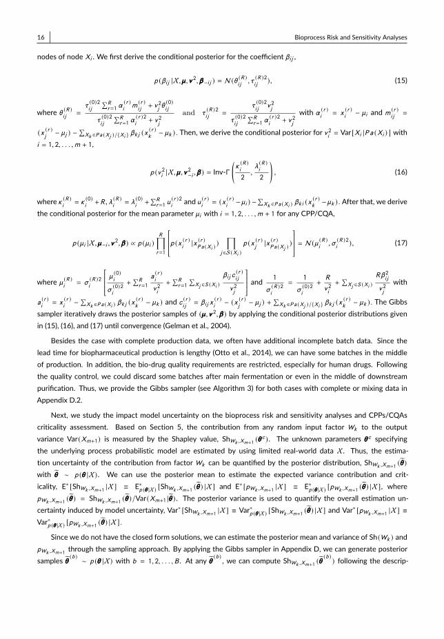
nodes of node Xi . We first derive the conditional posterior for the coefficient βi j ,
p (βi j |X,µµµ,vvv 2,βββ−i j ) = N(θ (R )i j, τ(R )2i j), (15)
where θ (R )i j
=τ(0)2i j
∑Rr=1 α
(r )im(r )i j
+ v 2jθ(0)i j
τ(0)2i j
∑Rr=1 α
(r )2i
+ v 2j
and τ(R )2i j
=τ(0)2i j
v 2j
τ(0)2i j
∑Rr=1 α
(r )2i
+ v 2j
with α (r )i
= x(r )i− µi and m (r )i j =
(x (r )j− µj ) −
∑Xk ∈P a (Xj )/{Xi } βk j (x
(r )k− µk ) . Then, we derive the conditional posterior for v 2i = Var[Xi |P a (Xi ) ] with
i = 1, 2, . . . ,m + 1,
p (v 2i |X,µµµ,vvv2−i ,βββ ) = Inv-Γ
(κ(R )i
2,λ(R )i
2
), (16)
where κ (R )i
= κ (0)i
+R , λ (R )i
= λ (0)i
+∑Rr=1 u
(r )2i
and u (r )i
= (x (r )i−µi ) −
∑Xk ∈P a (Xi ) βk i (x
(r )k−µk ) . After that, we derive
the conditional posterior for the mean parameter µi with i = 1, 2, . . . ,m + 1 for any CPP/CQA,
p (µi |X,µµµ−i ,vvv 2,βββ ) ∝ p (µi )R∏r=1
p (x (r )i |x (r )P a (Xi ) )∏
j ∈S(Xi )p (x (r )
j|x (r )P a (Xj )
) = N(µ (R )i
,σ(R )2i), (17)
where µ (R )i
= σ(R )2i
µ(0)i
σ(0)2i
+∑Rr=1
a(r )i
v 2i
+∑Rr=1
∑Xj ∈S (Xi )
βi j c(r )i j
v 2j
and 1
σ(R )2i
=1
σ(0)2i
+R
v 2i
+∑Xj ∈S (Xi )
Rβ 2i j
v 2j
with
a(r )i
= x (r )i− ∑
Xk ∈P a (Xi ) βk j (x(r )k− µk ) and c (r )i j = βi j x
(r )i− (x (r )
j− µj ) +
∑Xk ∈P a (Xj )/{Xi } βk j (x
(r )k− µk ) . The Gibbs
sampler iteratively draws the posterior samples of (µµµ,vvv 2,βββ ) by applying the conditional posterior distributions givenin (15), (16), and (17) until convergence (Gelman et al., 2004).
Besides the case with complete production data, we often have additional incomplete batch data. Since thelead time for biopharmaceutical production is lengthy (Otto et al., 2014), we can have some batches in the middleof production. In addition, the bio-drug quality requirements are restricted, especially for human drugs. Followingthe quality control, we could discard some batches after main fermentation or even in the middle of downstreampurification. Thus, we provide the Gibbs sampler (see Algorithm 3) for both cases with complete or mixing data inAppendix D.2.
Next, we study the impact model uncertainty on the bioprocess risk and sensitivity analyses and CPPs/CQAscriticality assessment. Based on Section 5, the contribution from any random input factor Wk to the outputvariance Var(Xm+1) is measured by the Shapley value, ShWk ,Xm+1 (θθθ
c ) . The unknown parameters θθθc specifyingthe underlying process probabilistic model are estimated by using limited real-world data X. Thus, the estima-tion uncertainty of the contribution from factor Wk can be quantified by the posterior distribution, ShWk ,Xm+1 (θθθ)with θθθ ∼ p (θθθ |X) . We can use the posterior mean to estimate the expected variance contribution and crit-icality, E∗ [ShWk ,Xm+1 |X] ≡ E∗p (θθθ |X) [ShWk ,Xm+1 (θθθ) |X] and E∗ [pWk ,Xm+1 |X] ≡ E∗p (θθθ |X) [pWk ,Xm+1 (θθθ) |X], wherepWk ,Xm+1 (θθθ) = ShWk ,Xm+1 (θθθ)/Var(Xm+1 |θθθ) . The posterior variance is used to quantify the overall estimation un-certainty induced by model uncertainty, Var∗ [ShWk ,Xm+1 |X] ≡ Var∗p (θθθ |X) [ShWk ,Xm+1 (θθθ) |X] and Var∗ [pWk ,Xm+1 |X] ≡Var∗p (θθθ |X) [pWk ,Xm+1 (θθθ) |X] .
Since we do not have the closed form solutions, we can estimate the posterior mean and variance of Sh(Wk ) andpWk ,Xm+1 through the sampling approach. By applying the Gibbs sampler in Appendix D, we can generate posteriorsamples θθθ (b ) ∼ p (θθθ |X) with b = 1, 2, . . . ,B . At any θθθ (b ) , we can compute ShWk ,Xm+1 (θθθ
(b ) ) following the descrip-
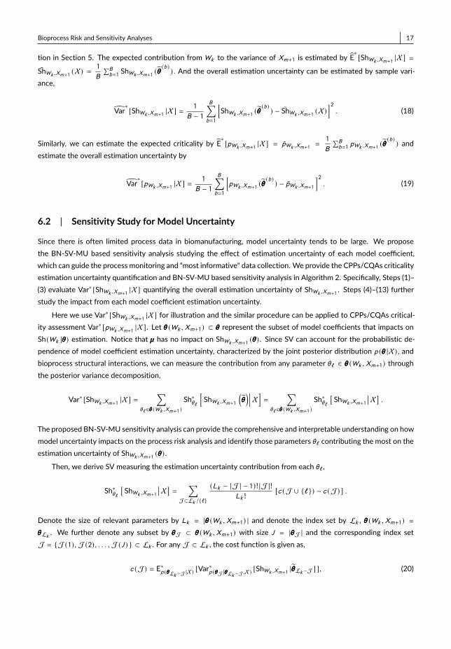
Bioprocess Risk and Sensitivity Analyses 17
tion in Section 5. The expected contribution fromWk to the variance of Xm+1 is estimated by E∗[ShWk ,Xm+1 |X] =
ShWk ,Xm+1 (X) =1
B
∑Bb=1 ShWk ,Xm+1 (θθθ
(b ) ) . And the overall estimation uncertainty can be estimated by sample vari-ance,
Var∗[ShWk ,Xm+1 |X] =
1
B − 1
B∑b=1
[ShWk ,Xm+1 (θθθ
(b ) ) − ShWk ,Xm+1 (X)]2. (18)
Similarly, we can estimate the expected criticality by E∗[pWk ,Xm+1 |X] = pWk ,Xm+1 =
1
B
∑Bb=1 pWk ,Xm+1 (θθθ
(b ) ) andestimate the overall estimation uncertainty by
Var∗[pWk ,Xm+1 |X] =
1
B − 1
B∑b=1
[pWk ,Xm+1 (θθθ
(b ) ) − pWk ,Xm+1]2. (19)
6.2 | Sensitivity Study for Model Uncertainty
Since there is often limited process data in biomanufacturing, model uncertainty tends to be large. We proposethe BN-SV-MU based sensitivity analysis studying the effect of estimation uncertainty of each model coefficient,which can guide the process monitoring and “most informative" data collection. We provide the CPPs/CQAs criticalityestimation uncertainty quantification and BN-SV-MU based sensitivity analysis in Algorithm 2. Specifically, Steps (1)–(3) evaluate Var∗ [ShWk ,Xm+1 |X] quantifying the overall estimation uncertainty of ShWk ,Xm+1 . Steps (4)–(13) furtherstudy the impact from each model coefficient estimation uncertainty.
Here we use Var∗ [ShWk ,Xm+1 |X] for illustration and the similar procedure can be applied to CPPs/CQAs critical-ity assessment Var∗ [pWk ,Xm+1 |X]. Let θθθ (Wk ,Xm+1) ⊂ θθθ represent the subset of model coefficients that impacts onSh(Wk |θθθ) estimation. Notice that µµµ has no impact on ShWk ,Xm+1 (θθθ) . Since SV can account for the probabilistic de-pendence of model coefficient estimation uncertainty, characterized by the joint posterior distribution p (θθθ |X) , andbioprocess structural interactions, we can measure the contribution from any parameter θ` ∈ θθθ (Wk ,Xm+1) throughthe posterior variance decomposition,
Var∗ [ShWk ,Xm+1 |X] =∑
θ` ∈θθθ (Wk ,Xm+1 )Sh∗θ`
[ShWk ,Xm+1
(θθθ)��� X]
=∑
θ` ∈θθθ (Wk ,Xm+1 )Sh∗θ`
[ShWk ,Xm+1
�� X].
The proposed BN-SV-MU sensitivity analysis can provide the comprehensive and interpretable understanding on howmodel uncertainty impacts on the process risk analysis and identify those parameters θ` contributing the most on theestimation uncertainty of ShWk ,Xm+1 (θθθ) .
Then, we derive SV measuring the estimation uncertainty contribution from each θ` ,
Sh∗θ`[ShWk ,Xm+1
�� X]=
∑J⊂Lk /{`}
(Lk − |J | − 1)! |J |!Lk !
[c (J ∪ {` }) − c (J) ] .
Denote the size of relevant parameters by Lk = |θθθ (Wk ,Xm+1) | and denote the index set by Lk , θθθ (Wk ,Xm+1) =θθθLk . We further denote any subset by θθθJ ⊂ θθθ (Wk ,Xm+1) with size J = |θθθJ | and the corresponding index setJ = {J (1), J(2), . . . , J(J ) } ⊂ Lk . For any J ⊂ Lk , the cost function is given as,
c (J) = E∗p (θθθLk −J |X)[Var∗p (θθθJ |θθθLk −J ,X)
[ShWk ,Xm+1 |θθθLk −J ] ], (20)
18 Bioprocess Risk and Sensitivity Analyses
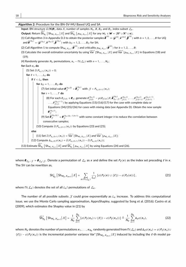
Algorithm 2: Procedure for the BN-SV-MU Based UQ and SAInput: BN structure G (N |θθθ) , data X, number of samples Nπ , B , BO and BI , index subset Lk .Output: Return Sh∗θ` [
ShWk ,Xm+1
�� X]and Sh
∗θ`
[pWk ,Xm+1
�� X]for anyWk ∈WWW = {Xp ∪ Xa ∪ e}.
(1) Call Algorithm 3 in Appendix D.3 to obtain the posterior samples θθθ (b ) = (µµµ (b ) , vvv (b )2, βββ (b ) ) with b = 1, 2, . . . ,B for UQand θθθ (bO ) = (µµµ (bO ) , vvv (bO )2, βββ (bO ) ) with bO = 1, 2, . . . ,BO for SA;
(2) Call Algorithm 1 to compute ShWk ,Xm+1 (θθθ(b ) ) and criticality pWk ,Xm+1 (θθθ
(b ) ) for b = 1, 2, . . . ,B ;(3) Calculate the overall estimation uncertainty by using Var
∗[ShWk ,Xm+1 |X] and Var
∗[pWk ,Xm+1 |X] in Equations (18) and
(19);(4) Randomly generate Nπ permutations, πn ∼ Π (Lk ) with n = 1, . . . ,Nπ ;for Each πn do
(5) Set c (Pπn (1) (πn )) = 0;for ` = 1, . . . , Lk do
if ` < Lk thenfor bO = 1, . . . ,BO do
(7) Set initial value θθθ (bO ,0)J = θθθ(bO )J with J = Pπn (`+1) (πn ) ;
for t = 1, . . . ,T do(8) For each θJ(` ) ∈ θθθJ , generate θ (bO ,t )J (` ) ∼ p (θJ(` ) |X, θθθ
(bO )Lk −J , θ
(bO ,t )J (1) , . . . , θ
(bO ,t )J (`−1) , θ
(bO ,t−1)J (`+1) ,
. . . , θ(bO ,t−1)J (J ) ) by applying Equations (15)/(16)/(17) for the case with complete data or
Equations (34)/(35)/(36) for cases with mixing data (see Appendix D). Obtain the new sampleθθθ(bO ,t )J ;
(9) Set θθθ (bO ,bI )J = θθθ (bO ,(bI −1)h+1)J with some constant integer h to reduce the correlation betweenconsecutive samples;
(10) Compute c (Pπn (`+1) (πn )) by Equations (23) and (25);else
(11) Set c (Pπn (`+1) (πn )) = Var∗[ShWk ,Xm+1 |X] and Var
∗[pWk ,Xm+1 |X];
(12) Compute ∆πn (` ) c (πn ) = c (Pπn (`+1) (πn )) − c (Pπn (` ) (πn )) ;
(13) Estimate Sh∗θ` [ShWk ,Xm+1
�� X]and Sh
∗θ`
[pWk ,Xm+1
�� X]by using Equations (24) and (26).
where θθθLk −J = θθθLk \J . Denote a permutation of Lk as π and define the set P` (π) as the index set preceding ` in π .The SV can be rewritten as,
Sh∗θ`[ShWk ,Xm+1
�� X]=
∑π∈Π (Lk )
1
Lk ![c (P` (π) ∪ {` }) − c (P` (π)) ] , (21)
where Π (Lk ) denotes the set of all Lk ! permutations of Lk .
The number of all possible subsets J could grow exponentially as Lk increase. To address this computationalissue, we use the Monte Carlo sampling approximation, ApproShapley, suggested by Song et al. (2016); Castro et al.(2009), which estimates the Shapley value in (21) by
Sh∗θ`
[ShWk ,Xm+1
�� X]=
1
Nπ
Nπ∑n=1
[c (P` (πn ) ∪ {` }) − c (P` (πn )) ] ,1
Nπ
Nπ∑n=1
∆`c (πn ), (22)
whereNπ denotes the number of permutations π1, . . . , πNπ randomly generated fromΠ (Lk ) and∆`c (πn ) = c (P` (πn )∪{` }) − c (P` (πn )) is the incremental posterior variance Var∗ [ShWk ,Xm+1 |X] induced by including the `-th model pa-
Bioprocess Risk and Sensitivity Analyses 19
rameter in P` (πn ) .As c (J) in (20) is analytically intractable, we develop Monte Carlo sampling estimation. However, since
the posterior samples obtained from the Gibbs sampler in Appendix D.3 cannot be directly used to estimateE∗p (θθθLk −J |X)
[Var∗p (θθθJ |θθθLk −J ,X)[ShWk ,Xm+1 |θθθLk −J ] ], we introduce a nested Gibbs sampling approach. For the “outer"
samples used to estimate E∗p (θθθLk −J |X)[ ·], the posterior samples θθθ (bO )Lk −J with bO = 1, . . . ,BO can be directly obtained
by applying the Gibbs sampling in Appendix D.3. We generate θθθ (bO ) ∼ p (θθθ |X) and keep components with indexLk − J. Then, at each θθθ
(bO )Lk −J , a conditional sampling is further developed to generate samples from p (θθθJ |θθθ
(bO )Lk −J , X) .
More specifically, we set the initial value θθθ (bO ,0)J = θθθ(bO )J . In each t -th MCMC iteration, given the previous sample
θθθ(bO ,t−1)J , we apply the Gibbs sampling to sequentially generate one sample from the conditional posterior for eachθJ(` ) ∈ θθθJ with ` = 1, . . . , |J |,
θ(bO ,t )J (` ) ∼ p
(θJ(` )
���X, θθθ (bO )Lk −J , θ(bO ,t )J (1) , . . . , θ
(bO ,t )J (`−1) , θ
(bO ,t−1)J (`+1) , . . . , θ
(bO ,t−1)J (|J|)
).
By repeating this procedure, we can get samples θθθ (bO ,t )J with t = 0, . . . ,T . We keep one for every h samples to reduce
the correlations between consecutive samples. Consequently, we obtain “inner" samples θθθ (bO ,bI )J with bI = 1, . . . ,BIto estimate Var∗p (θθθJ |θθθLk −J ,X)
[ShWk ,Xm+1 |θθθLk −J ].
Thus, this nested Gibbs sampling can generate BO · BI samples {(θθθ (bO ,bI )J , θθθ(bO )Lk −J ) : bO = 1, . . . ,BO and bI =
1, . . . ,BI } to estimate c (J) in (20). For any J ⊂ Lk , the cost function can be estimated as,
c (J) = 1
BO
BO∑bO =1
1
BI − 1
BI∑bI =1
[ShWk ,Xm+1 (θθθ
(bO ,bI )J , θθθ
(bO )Lk −J ) − ShWk ,Xm+1 (θθθ
(bO )Lk −J )
]2 , (23)
where ShWk ,Xm+1 (θθθ(bO )Lk −J ) =
∑BIbI =1
ShWk ,Xm+1 (θθθ(bO ,bI )J , θθθ
(bO )Lk −J )/BI . By plugging c (J) into Equation (22), we can
quantify the estimation uncertainty contribution from each model coefficient θ` ∈ θθθLk ,
Sh∗θ` [ShWk ,Xm+1
�� X]=
1
Nπ
Nπ∑n=1
∆` c (πn ), (24)
where ∆` c (πn ) = c (P` (πn ) ∪ {` }) − c (P` (πn )) for all ` = 1, . . . , Lk . Similarly, for CPP/CQA criticality assessment, wecan estimate the cost function,
c′ (J) = 1
BO
BO∑bO =1
1
BI − 1
BI∑bI =1
[pWk ,Xm+1 (θθθ
(bO ,bI )J , θθθ
(bO )Lk −J ) − pWk ,Xm+1 (θθθ
(bO )Lk −J )
]2 , (25)
where pWk ,Xm+1 (θθθ(bO )Lk −J ) =
∑BIbI =1
pWk ,Xm+1 (θθθ(bO ,bI )J , θθθ
(bO )Lk −J )/BI . Then, we estimate the estimation uncertainty con-
tribution from θ` on the criticality assessement,
Sh∗θ`
[pWk ,Xm+1
�� X]=
1
Nπ
Nπ∑n=1
∆` c′ (πn ) . (26)
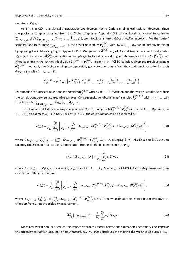
More real-world data can reduce the impact of process model coefficient estimation uncertainty and improvethe criticality estimation accuracy of input factors, sayWk , that contribute the most to the variance of output Xm+1.
20 Bioprocess Risk and Sensitivity Analyses
This study can guide the “most informative" data collection. Basically, we can focus on the dominant criticality mea-surements with high estimation uncertainty induced by model uncertainty, assessed by variance Var
∗[ShWk ,Xm+1 |X]
in Equation (18), or Var∗[pWk ,Xm+1 |X] in Equation (19). Given the real-world data X, the proportion of estimation
uncertainty contributed from each coefficient θ` ∈ θθθ (Wk ,Xm+1) can be estimated by,
p∗θ`[ShWk ,Xm+1
�� X]=
Sh∗θ` [ShWk ,Xm+1
�� X]Var∗[ShWk ,Xm+1 |X]
, or p∗θ`[pWk ,Xm+1
�� X]=
Sh∗θ`
[pWk ,Xm+1
�� X]Var∗[pWk ,Xm+1 |X]
.
By ranking the proportional contribution, we can find the coefficient θ` with the highest contribution, which canguide the collection of the most informative data to control the impact of model estimation uncertainty and supportproduction process risk analysis. We will study the impact of additional data collection and provide a systematic andrigorous approach to guide efficient data collection in the future research.
7 | EMPIRICAL STUDY
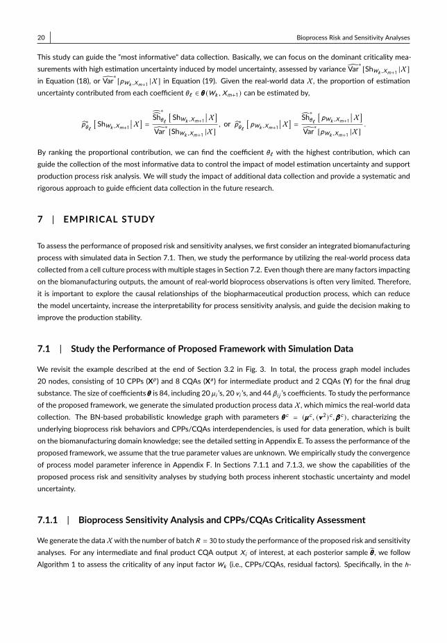
To assess the performance of proposed risk and sensitivity analyses, we first consider an integrated biomanufacturingprocess with simulated data in Section 7.1. Then, we study the performance by utilizing the real-world process datacollected from a cell culture process with multiple stages in Section 7.2. Even though there are many factors impactingon the biomanufacturing outputs, the amount of real-world bioprocess observations is often very limited. Therefore,it is important to explore the causal relationships of the biopharmaceutical production process, which can reducethe model uncertainty, increase the interpretability for process sensitivity analysis, and guide the decision making toimprove the production stability.
7.1 | Study the Performance of Proposed Framework with Simulation Data
We revisit the example described at the end of Section 3.2 in Fig. 3. In total, the process graph model includes20 nodes, consisting of 10 CPPs (Xp ) and 8 CQAs (Xa ) for intermediate product and 2 CQAs (Y) for the final drugsubstance. The size of coefficients θθθ is 84, including 20 µi ’s, 20 vi ’s, and 44 βi j ’s coefficients. To study the performanceof the proposed framework, we generate the simulated production process data X, which mimics the real-world datacollection. The BN-based probabilistic knowledge graph with parameters θθθc = (µµµc , (vvv 2)c ,βββ c ) , characterizing theunderlying bioprocess risk behaviors and CPPs/CQAs interdependencies, is used for data generation, which is builton the biomanufacturing domain knowledge; see the detailed setting in Appendix E. To assess the performance of theproposed framework, we assume that the true parameter values are unknown. We empirically study the convergenceof process model parameter inference in Appendix F. In Sections 7.1.1 and 7.1.3, we show the capabilities of theproposed process risk and sensitivity analyses by studying both process inherent stochastic uncertainty and modeluncertainty.
7.1.1 | Bioprocess Sensitivity Analysis and CPPs/CQAs Criticality Assessment
Wegenerate the data Xwith the number of batch R = 30 to study the performance of the proposed risk and sensitivityanalyses. For any intermediate and final product CQA output Xi of interest, at each posterior sample θθθ, we followAlgorithm 1 to assess the criticality of any input factorWk (i.e., CPPs/CQAs, residual factors). Specifically, in the h-
Bioprocess Risk and Sensitivity Analyses 21
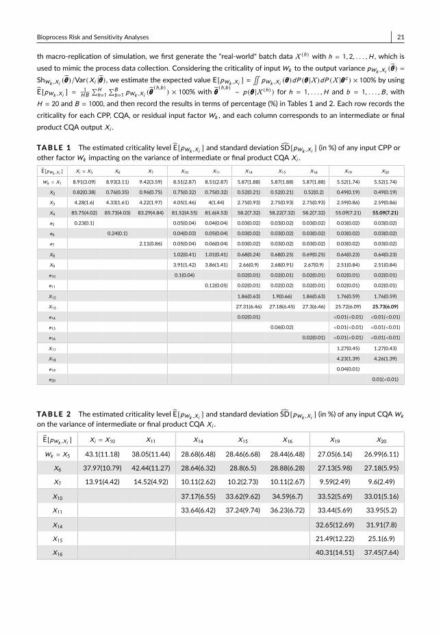
th macro-replication of simulation, we first generate the “real-world" batch data X (h) with h = 1, 2, . . . ,H , which isused to mimic the process data collection. Considering the criticality of inputWk to the output variance pWk ,Xi (θθθ) =ShWk ,Xi (θθθ)/Var(Xi |θθθ) , we estimate the expected value E[pWk ,Xi ] =
∬pWk ,Xi (θθθ)dP (θθθ |X)dP (X |θθθ
c ) × 100% by usingE[pWk ,Xi ] =
1HB
∑Hh=1
∑Bb=1 pWk ,Xi (θθθ
(h,b ) ) × 100% with θθθ (h,b ) ∼ p (θθθ |X (h) ) for h = 1, . . . ,H and b = 1, . . . ,B , withH = 20 and B = 1000, and then record the results in terms of percentage (%) in Tables 1 and 2. Each row records thecriticality for each CPP, CQA, or residual input factorWk , and each column corresponds to an intermediate or finalproduct CQA output Xi .
TABLE 1 The estimated criticality level E[pWk ,Xi ] and standard deviation SD[pWk ,Xi ] (in %) of any input CPP orother factorWk impacting on the variance of intermediate or final product CQA Xi .E[pWk ,Xi ] Xi = X5 X6 X7 X10 X11 X14 X15 X16 X19 X20
Wk = X1 8.91(3.09) 8.93(3.11) 9.42(3.59) 8.51(2.87) 8.51(2.87) 5.87(1.88) 5.87(1.88) 5.87(1.88) 5.52(1.74) 5.52(1.74)
X2 0.82(0.38) 0.76(0.35) 0.96(0.75) 0.75(0.32) 0.75(0.32) 0.52(0.21) 0.52(0.21) 0.52(0.2) 0.49(0.19) 0.49(0.19)
X3 4.28(1.6) 4.33(1.61) 4.22(1.97) 4.05(1.46) 4(1.44) 2.75(0.93) 2.75(0.93) 2.75(0.93) 2.59(0.86) 2.59(0.86)
X4 85.75(4.02) 85.73(4.03) 83.29(4.84) 81.52(4.55) 81.6(4.53) 58.2(7.32) 58.22(7.32) 58.2(7.32) 55.09(7.21) 55.09(7.21)
e5 0.23(0.1) 0.05(0.04) 0.04(0.04) 0.03(0.02) 0.03(0.02) 0.03(0.02) 0.03(0.02) 0.03(0.02)
e6 0.24(0.1) 0.04(0.03) 0.05(0.04) 0.03(0.02) 0.03(0.02) 0.03(0.02) 0.03(0.02) 0.03(0.02)
e7 2.11(0.86) 0.05(0.04) 0.06(0.04) 0.03(0.02) 0.03(0.02) 0.03(0.02) 0.03(0.02) 0.03(0.02)
X8 1.02(0.41) 1.01(0.41) 0.68(0.24) 0.68(0.25) 0.69(0.25) 0.64(0.23) 0.64(0.23)
X9 3.91(1.42) 3.86(1.41) 2.66(0.9) 2.68(0.91) 2.67(0.9) 2.51(0.84) 2.51(0.84)
e10 0.1(0.04) 0.02(0.01) 0.02(0.01) 0.02(0.01) 0.02(0.01) 0.02(0.01)
e11 0.12(0.05) 0.02(0.01) 0.02(0.02) 0.02(0.01) 0.02(0.01) 0.02(0.01)
X12 1.86(0.63) 1.9(0.66) 1.86(0.63) 1.76(0.59) 1.76(0.59)
X13 27.31(6.46) 27.18(6.45) 27.3(6.46) 25.72(6.09) 25.73(6.09)
e14 0.02(0.01) <0.01(<0.01) <0.01(<0.01)
e15 0.06(0.02) <0.01(<0.01) <0.01(<0.01)
e16 0.02(0.01) <0.01(<0.01) <0.01(<0.01)
X17 1.27(0.45) 1.27(0.43)
X18 4.23(1.39) 4.26(1.39)
e19 0.04(0.01)
e20 0.01(<0.01)
TABLE 2 The estimated criticality level E[pWk ,Xi ] and standard deviation SD[pWk ,Xi ] (in %) of any input CQAWk
on the variance of intermediate or final product CQA Xi .
E[pWk ,Xi ] Xi = X10 X11 X14 X15 X16 X19 X20
Wk = X5 43.1(11.18) 38.05(11.44) 28.68(6.48) 28.46(6.68) 28.44(6.48) 27.05(6.14) 26.99(6.11)
X6 37.97(10.79) 42.44(11.27) 28.64(6.32) 28.8(6.5) 28.88(6.28) 27.13(5.98) 27.18(5.95)
X7 13.91(4.42) 14.52(4.92) 10.11(2.62) 10.2(2.73) 10.11(2.67) 9.59(2.49) 9.6(2.49)
X10 37.17(6.55) 33.62(9.62) 34.59(6.7) 33.52(5.69) 33.01(5.16)
X11 33.64(6.42) 37.24(9.74) 36.23(6.72) 33.44(5.69) 33.95(5.2)
X14 32.65(12.69) 31.91(7.8)
X15 21.49(12.22) 25.1(6.9)
X16 40.31(14.51) 37.45(7.64)

22 Bioprocess Risk and Sensitivity Analyses
The process model uncertainty is characterized by the posterior p (θθθ |X) and the overall impact on the CPPs/CQAs criti-cality assessment can be quantified by the posterior standard deviation (SD), SD∗ [pWk ,Xi (θθθ) |X]. Based on the results from
H macro-replications, we compute the expected SD for criticality estimation, SD[pWk ,Xi ] =√E[Var∗ (pWk ,Xi (θθθ) |X) ]×
100%, with the estimate,
SD[pWk ,Xi ] =
√√√1
H (B − 1)
H∑h=1
B∑b=1
[pWk ,Xi
(θθθ(h,b ) ) − p (h)
Wk ,Xi
]2× 100%
where p (h)Wk ,Xi
= 1B
∑Bb=1 pWk ,Xi (θθθ
(h,b ) ) . In Tables 1 and 2, we record the results of SD in terms of percentage (%) in thebracket.
For each CQA output Xi , we record the criticality with the estimated mean E[pWk ,Xi ] and standard deviationSD[pWk ,Xi ] from any CPP or other factorWk in Table 1. Under the example setting, we can see that the variationsin X4 (dissolved oxygen in main fermentation) and X13 (temperature in chromatography) have the dominant impacton both intermediate and final product CQAs’ variance. Compared with main fermentation and chromatography,the other two operation units (i.e., centrifuge and filtration) have relatively small impact on the final product qualityvariation. Based on the process risk and sensitivity analyses, we also provide the result visualization; see for exampleFig. 3.
By studying the subplots of the bioprocess probabilistic knowledge graph illustrated in Fig. 3, we can study thecontributions from the dependent CQAs of intermediate products as inputs to the variance of final drug substanceCQAs outputs, i.e., nodes {X19,X20 }. We consider the subplots: (1) starting from the end of main fermentation with{X5,X6,X7 }; (2) starting from the end of centrifuge with {X10,X11 }; and (3) starting from the end of chromatogra-phy with {X14,X15,X16 }. The results of process sensitivity analysis are recorded in Table 2. The CQAs after mainfermentation, i.e., {X5,X6,X7 }, together account for about 50% variance of final output X19 or X20; and CQAs af-ter chromatography, i.e., {X14,X15,X16 } together account for about 90% of final output variation. Thus, the CQAs ofintermediate product close to the end of production process provides better explanation of the variation of final drug sub-stance CQAs and we can predict more accurate on its productivity and quality. This information can be used to guide theproduction process quality control and support the real-time release.
7.1.2 | Criticality Assessment Estimation Performance Comparison
In this section, we use the same example studied in Section 7.1.1 to compare the performance of criticality assessmentobtained by the proposed BN-SV approach (denoted by pBN−SV
Wk ,X20) with an existing approach, which uses multiple
linear regression and Morris sensitivity analysis (represented by ML-M); see Hassan et al. (2013); Zi (2011); Helton(1993). Basically, we first fit the multiple linear regression to the random inputs (i.e., Wk = Xi listed in the firstcolumn of Table 1) and output X20, and then use Morris sensitivity analysis to measure the criticality of each inputWk . Here, we use the same experiment setting with that used in Section 7.1.1. With the underlying parameterssetting θθθc = (µµµc , (vvv 2)c ,βββ c ) given in Appendix E, the true criticality of any input factor Wk can be calculated withpcWk ,X20
= ShWk ,X20 (θθθc )/Var(X20 |θθθc ) , where ShWk ,X20 (θθθ
c ) and Var(X20 |θθθc ) are obtained by applying Equations (11)and (12). Then, suppose the underlying process model coefficients are unknown, and we can compare the criticalityassessment performance of both approaches. In Table 3, we record the mean and SD of criticality estimates obtainedfrom LM-M and proposed BN-SV approaches with H = 30macro-replications and R = 30 batches. The mean absolute

Bioprocess Risk and Sensitivity Analyses 23
error (MAE) is calculated by,
MAE (pγWk ,X20
) = 1
HB
H∑h=1
B∑b=1
���pγWk ,X20 (θθθ (h,b ) ) − pcWk ,X20 ��� × 100% (27)
where γ is ML-M or BN-SV. The results in Table 3 show that the proposed BN-SV sensitivity analysis provides bettercriticality assessment of critical inputs.
TABLE 3 The CPPs criticality estimation results obtained by BN-SV sensitivity analysis and existing multipleregression based sensitivity analysis.
Criticality (%) True Value pcWk ,X20pML−MWk ,X20
MAE pBN−SVWk ,X20MAE
Wk = X4 59.55 56.91 (14.94) 11.14 55.09 (7.21) 7.86
X13 24.01 26.06 (9.47) 6.41 25.73 (6.09) 5.19
X1 4.67 5.40 (1.63) 1.24 5.52 (1.74) 1.41
X18 3.66 4.25 (1.64) 1.21 4.26 (1.39) 1.13
X3 2.38 2.55 (0.77) 0.61 2.59 (0.86) 0.47
X9 2.16 2.36 (0.77) 0.64 2.51 (0.84) 0.68
X12 1.5 1.73 (0.52) 0.45 1.76 (0.59) 0.42
X17 1.04 1.25 (0.59) 0.43 1.27 (0.43) 0.35
7.1.3 | Sensitivity Analysis for Model Uncertainty
Here we consider the product protein content X20 in Fig. 3 as the output to study the performance of sensitivityanalysis for model uncertainty. Based on the results in Table 1, the CPPs X4 and X13 have the dominant contributionsto the variance of outputX20, and the estimates of pWk ,Xi also have the high estimation uncertainty. Thus, we conductthe BN-SV-MU sensitivity analysis to study how the estimation uncertainty of each model coefficient impacts on thecriticality assessment for pX4,X20 and pX13,X20 .
Given the data X, we provide the posterior variance decomposition studying the criticality estimation uncertaintyinduced by theMU, Var∗p (θθθ |X) [pWk ,Xi (θθθ) |X] =
∑θ` ∈θθθ (Wk ,Xi ) Sh
∗θ`
[pWk ,Xi (θθθ)
��� X]. Then, we can estimate the expected
relative contribution from each model coefficient θ` ∈ θθθ (Wk ,Xi ) with EPθ` (pWk ,Xi ) ≡ E[
Sh∗θ`[pWk ,Xi
(θθθ)���X]
Var∗p (θθθ |X)[pWk ,Xi
(θθθ)���X] ] .
In the h-th macro-replication, given the data X (h) , we can estimate the contribution from each θ` by usingSh∗θ` [pWk ,Xi (θθθ)
��� X (h) ] and Var∗p (θθθ |X)
[pWk ,Xi (θθθ)
��� X (h) ] following Equations (24) and (19), which is estimated by us-ing Nπ = 500, BO = 5 and BI = 20; see Song et al. (2016) for the selection of sampling parameter setting. Thus, we
have the estimation uncertainty proportion EPθ` (pWk ,Xi ) ≡1H
∑Hh=1
Sh∗θ` [pWk ,Xi
(θθθ)���X (h) ]
Var∗p (θθθ |X)[pWk ,Xi
(θθθ)���X (h) ] with H = 20.
The coefficients contributing to the estimation of ShX4,X20 include v 24 and 18 linear coefficients βββ on the pathsfrom node X4 to node X20. The coefficients contributing to the estimation of ShX13,X20 include v 213 and 6 linear co-efficients βββ located on the paths from X13 to X20. Due to the space limit, we only present the top five coefficientscontributing most to the estimation uncertainty of criticality pX4,X20 and pX13,X20 , and aggregate the results for re-maining coefficients. The sensitivity analysis results, EPθ` (pWk ,Xi ) ± SE
[EPθ` (pWk ,Xi )
], for pX4,X20 and pX13,X20 are
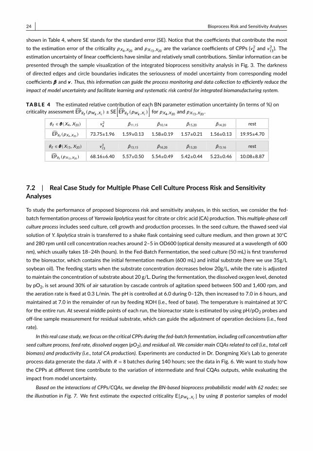
24 Bioprocess Risk and Sensitivity Analyses
shown in Table 4, where SE stands for the standard error (SE). Notice that the coefficients that contribute the mostto the estimation error of the criticality pX4,X20 and pX13,X20 are the variance coefficients of CPPs (v 24 and v 213). Theestimation uncertainty of linear coefficients have similar and relatively small contributions. Similar information can bepresented through the sample visualization of the integrated bioprocess sensitivity analysis in Fig. 3. The darknessof directed edges and circle boundaries indicates the seriousness of model uncertainty from corresponding modelcoefficients βββ and vvv . Thus, this information can guide the process monitoring and data collection to efficiently reduce theimpact of model uncertainty and facilitate learning and systematic risk control for integrated biomanufacturing system.
TABLE 4 The estimated relative contribution of each BN parameter estimation uncertainty (in terms of %) oncriticality assessment EPθ` (pWk ,Xi ) ± SE
[EPθ` (pWk ,Xi )
]for pX4,X20 and pX13,X20 .
θ` ∈ θθθ (X4,X20) v 24 β11,15 β10,14 β15,20 β14,20 rest
EPθ` (pX4,X20 ) 73.75±1.96 1.59±0.13 1.58±0.19 1.57±0.21 1.56±0.13 19.95±4.70
θ` ∈ θθθ (X13,X20) v 213 β13,15 β16,20 β15,20 β13,16 rest
EPθ` (pX13,X20 ) 68.16±6.40 5.57±0.50 5.54±0.49 5.42±0.44 5.23±0.46 10.08±8.87
7.2 | Real Case Study for Multiple Phase Cell Culture Process Risk and SensitivityAnalyses
To study the performance of proposed bioprocess risk and sensitivity analyses, in this section, we consider the fed-batch fermentation process of Yarrowia lipolytica yeast for citrate or citric acid (CA) production. Thismultiple-phase cellculture process includes seed culture, cell growth and production processes. In the seed culture, the thawed seed vialsolution of Y. lipolytica strain is transferred to a shake flask containing seed culture medium, and then grown at 30°Cand 280 rpm until cell concentration reaches around 2–5 in OD600 (optical density measured at a wavelength of 600nm), which usually takes 18–24h (hours). In the Fed-Batch Fermentation, the seed culture (50 mL) is first transferredto the bioreactor, which contains the initial fermentation medium (600 mL) and initial substrate (here we use 35g/Lsoybean oil). The feeding starts when the substrate concentration decreases below 20g/L, while the rate is adjustedtomaintain the concentration of substrate about 20 g/L. During the fermentation, the dissolved oxygen level, denotedby pO2, is set around 30% of air saturation by cascade controls of agitation speed between 500 and 1,400 rpm, andthe aeration rate is fixed at 0.3 L/min. The pH is controlled at 6.0 during 0–12h, then increased to 7.0 in 6 hours, andmaintained at 7.0 in the remainder of run by feeding KOH (i.e., feed of base). The temperature is maintained at 30°Cfor the entire run. At several middle points of each run, the bioreactor state is estimated by using pH/pO2 probes andoff-line sample measurement for residual substrate, which can guide the adjustment of operation decisions (i.e., feedrate).
In this real case study, we focus on the critical CPPs during the fed-batch fermentation, including cell concentration afterseed culture process, feed rate, dissolved oxygen (pO2), and residual oil. We consider main CQAs related to cell (i.e., total cellbiomass) and productivity (i.e., total CA production). Experiments are conducted in Dr. Dongming Xie’s Lab to generateprocess data generate the data X with R = 8 batches during 140 hours; see the data in Fig. 6. We want to study howthe CPPs at different time contribute to the variation of intermediate and final CQAs outputs, while evaluating theimpact from model uncertainty.
Based on the interactions of CPPs/CQAs, we develop the BN-based bioprocess probabilistic model with 62 nodes; seethe illustration in Fig. 7. We first estimate the expected criticality E[pWk ,Xi ] by using B posterior samples of model
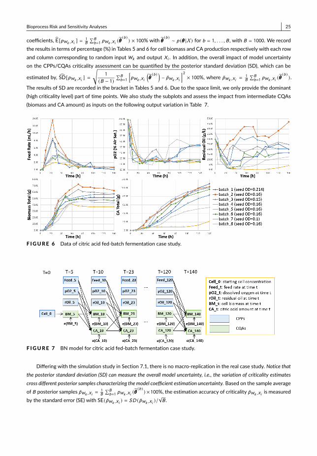
Bioprocess Risk and Sensitivity Analyses 25
coefficients, E[pWk ,Xi ] =1B
∑Bb=1 pWk ,Xi (θθθ
(b ) ) × 100% with θθθ (b ) ∼ p (θθθ |X) for b = 1, . . . ,B , with B = 1000. We recordthe results in terms of percentage (%) in Tables 5 and 6 for cell biomass and CA production respectively with each rowand column corresponding to random inputWk and output Xi . In addition, the overall impact of model uncertaintyon the CPPs/CQAs criticality assessment can be quantified by the posterior standard deviation (SD), which can be
estimated by, SD[pWk ,Xi ] =
√1
(B − 1)∑Bb=1
[pWk ,Xi
(θθθ(b ) ) − pWk ,Xi ]2 × 100%, where pWk ,Xi =
1B
∑Bb=1 pWk ,Xi (θθθ
(b ) ) .
The results of SD are recorded in the bracket in Tables 5 and 6. Due to the space limit, we only provide the dominant(high criticality level) part of time points. We also study the subplots and assess the impact from intermediate CQAs(biomass and CA amount) as inputs on the following output variation in Table 7.
F IGURE 6 Data of citric acid fed-batch fermentation case study.
F IGURE 7 BN model for citric acid fed-batch fermentation case study.
Differing with the simulation study in Section 7.1, there is no macro-replication in the real case study. Notice thatthe posterior standard deviation (SD) can measure the overall model uncertainty, i.e., the variation of criticality estimatescross different posterior samples characterizing the model coefficient estimation uncertainty. Based on the sample averageof B posterior samples pWk ,Xi =
1B
∑Bb=1 pWk ,Xi (θθθ
(b ) ) ×100%, the estimation accuracy of criticality pWk ,Xi is measuredby the standard error (SE) with SE(pWk ,Xi ) = SD (pWk ,Xi )/
√B .
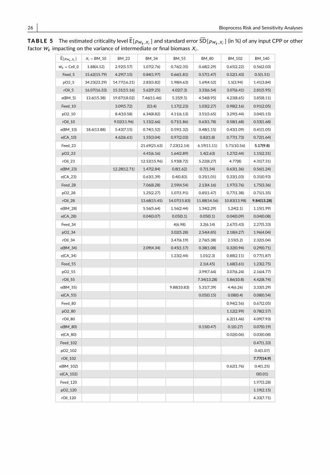
26 Bioprocess Risk and Sensitivity Analyses
TABLE 5 The estimated criticality level E[pWk ,Xi ] and standard error SD[pWk ,Xi ] (in %) of any input CPP or otherfactorWk impacting on the variance of intermediate or final biomass Xi .
E[pWk ,Xi ] Xi = BM_10 BM_23 BM_34 BM_55 BM_80 BM_102 BM_140
Wk = Cell_0 1.88(4.12) 2.92(5.57) 1.07(2.76) 0.76(2.35) 0.68(2.29) 0.65(2.22) 0.56(2.03)
Feed_5 15.62(15.79) 4.29(7.15) 0.84(1.97) 0.66(1.81) 0.57(1.47) 0.52(1.43) 0.5(1.51)
pO2_5 34.23(22.29) 14.77(16.21) 2.83(5.82) 1.98(4.63) 1.69(4.52) 1.5(3.94) 1.41(3.84)
rOil_5 16.07(16.33) 15.31(15.16) 5.62(9.25) 4.02(7.3) 3.33(6.54) 3.07(6.41) 2.81(5.95)
e(BM_5) 13.6(15.38) 19.87(18.02) 7.46(11.46) 5.35(9.5) 4.54(8.95) 4.23(8.65) 3.85(8.11)
Feed_10 3.09(5.72) 2(3.4) 1.17(2.23) 1.03(2.27) 0.98(2.16) 0.91(2.05)
pO2_10 8.4(10.58) 6.34(8.82) 4.11(6.13) 3.51(5.65) 3.29(5.44) 3.04(5.15)
rOil_10 9.02(11.96) 1.15(2.66) 0.71(1.86) 0.63(1.78) 0.58(1.68) 0.53(1.68)
e(BM_10) 18.6(13.88) 5.43(7.15) 0.74(1.52) 0.59(1.32) 0.48(1.15) 0.43(1.09) 0.41(1.05)
e(CA_10) 4.62(6.61) 1.55(3.04) 0.97(2.03) 0.82(1.8) 0.77(1.73) 0.72(1.64)
Feed_23 21.69(21.63) 7.23(12.14) 6.19(11.11) 5.71(10.56) 5.17(9.8)
pO2_23 4.41(6.16) 1.64(2.89) 1.4(2.63) 1.27(2.44) 1.15(2.31)
rOil_23 12.52(15.96) 5.93(8.72) 5.22(8.27) 4.77(8) 4.31(7.31)
e(BM_23) 12.28(12.71) 1.47(2.84) 0.8(1.62) 0.7(1.54) 0.63(1.36) 0.56(1.24)
e(CA_23) 0.63(1.39) 0.4(0.83) 0.35(1.01) 0.33(1.03) 0.31(0.93)
Feed_28 7.06(8.28) 2.59(4.54) 2.13(4.16) 1.97(3.76) 1.75(3.36)
pO2_28 1.25(2.27) 1.07(1.91) 0.85(1.47) 0.77(1.38) 0.71(1.35)
rOil_28 13.68(15.45) 14.07(15.83) 11.88(14.56) 10.83(13.98) 9.84(13.28)
e(BM_28) 5.56(5.64) 1.56(2.44) 1.34(2.29) 1.24(2.1) 1.15(1.99)
e(CA_28) 0.04(0.07) 0.05(0.1) 0.05(0.1) 0.04(0.09) 0.04(0.08)
Feed_34 4(6.98) 3.2(6.14) 2.67(5.43) 2.27(5.33)
pO2_34 3.02(5.28) 2.54(4.85) 2.18(4.27) 1.96(4.04)
rOil_34 3.47(6.19) 2.76(5.38) 2.55(5.2) 2.32(5.04)
e(BM_34) 2.09(4.34) 0.45(1.17) 0.38(1.08) 0.32(0.94) 0.29(0.71)
e(CA_34) 1.23(2.44) 1.01(2.3) 0.88(2.11) 0.77(1.87)
Feed_55 2.1(4.45) 1.68(3.61) 1.23(2.75)
pO2_55 3.99(7.64) 3.07(6.24) 2.16(4.77)
rOil_55 7.34(13.28) 5.86(10.8) 4.42(8.74)
e(BM_55) 9.88(10.83) 5.31(7.39) 4.4(6.26) 3.33(5.29)
e(CA_55) 0.05(0.15) 0.08(0.4) 0.08(0.54)
Feed_80 0.94(2.56) 0.67(2.05)
pO2_80 1.12(2.99) 0.78(2.57)
rOil_80 6.2(11.46) 4.09(7.93)
e(BM_80) 0.15(0.47) 0.1(0.27) 0.07(0.19)
e(CA_80) 0.02(0.06) 0.03(0.08)
Feed_102 0.47(1.33)
pO2_102 0.4(1.07)
rOil_102 7.77(14.9)
e(BM_102) 0.62(1.76) 0.4(1.25)
e(CA_102) 0(0.01)
Feed_120 1.97(3.28)
pO2_120 1.19(2.15)
rOil_120 4.33(7.71)
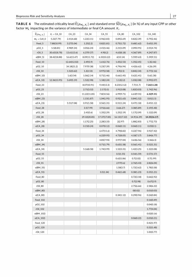
Bioprocess Risk and Sensitivity Analyses 27
TABLE 6 The estimated criticality level E[pWk ,Xi ] and standard error SD[pWk ,Xi ] (in %) of any input CPP or otherfactorWk impacting on the variance of intermediate or final CA amount Xi .
E[pWk ,Xi ] Xi = CA_10 CA_23 CA_34 CA_55 CA_80 CA_102 CA_140
Wk = Cell_0 5.22(7.79) 2.41(4.68) 1.22(3.11) 0.96(2.83) 0.89(2.69) 0.82(2.39) 0.79(2.46)
Feed_5 7.88(10.99) 3.27(5.04) 1.25(2.2) 0.82(1.81) 0.75(1.72) 0.68(1.62) 0.65(1.59)
pO2_5 5.5(8.81) 4.98(9.24) 3.05(6.24) 2.41(5.46) 2.21(5.09) 2.09(4.95) 2.01(4.74)
rOil_5 30.63(18.78) 13.61(13.6) 6.37(9.37) 4.9(8.2) 4.63(8.18) 4.36(7.89) 4.24(7.87)
e(BM_5) 38.42(18.88) 16.6(15.47) 8.09(11.72) 6.33(10.22) 6(10.14) 5.59(9.63) 5.39(9.51)
Feed_10 12.64(12.02) 2.49(3.9) 1.61(2.76) 1.45(2.53) 1.35(2.45) 1.3(2.46)
pO2_10 34.18(21.2) 7.97(9.38) 5.23(7.39) 4.79(6.94) 4.42(6.62) 4.2(6.39)
rOil_10 1.52(3.62) 1.2(2.53) 0.97(2.58) 0.9(2.5) 0.84(2.34) 0.77(2.16)
e(BM_10) 1.6(3.54) 1.06(2.14) 0.71(1.46) 0.66(1.45) 0.62(1.41) 0.6(1.38)
e(CA_10) 12.36(13.95) 3.69(5.19) 1.52(2.98) 1.18(2.24) 1.12(2.2) 1.03(2.08) 0.99(2.07)
Feed_23 8.07(10.91) 9.44(13.3) 8.23(12.12) 7.7(11.7) 7.26(11.28)
pO2_23 2.71(3.52) 2.17(3.5) 1.91(3.08) 1.82(3.03) 1.74(2.96)
rOil_23 11.22(11.85) 7.8(10.56) 6.99(9.71) 6.63(9.55) 6.32(9.31)
e(BM_23) 1.15(1.87) 1.04(1.95) 0.92(1.63) 0.84(1.52) 0.81(1.5)
e(CA_23) 5.51(7.08) 0.91(1.58) 0.56(1.31) 0.51(1.24) 0.47(1.18) 0.45(1.12)
Feed_28 3.5(7.99) 3.91(6.66) 3.6(6.27) 3.38(5.89) 3.19(5.48)
pO2_28 2.43(3.6) 1.35(2.29) 1.25(2.19) 1.17(2.09) 1.12(2.09)
rOil_28 29.32(20.85) 17.37(17.85) 16.13(17.22) 14.9(16.39) 14.35(16.17)
e(BM_28) 1.17(2.25) 2.28(3.33) 2(2.97) 1.88(2.83) 1.77(2.73)
e(CA_28) 0.15(0.24) 0.07(0.12) 0.06(0.11) 0.06(0.11) 0.05(0.1)
Feed_34 6.47(11.6) 4.79(8.82) 4.22(7.96) 3.92(7.42)
pO2_34 6.22(9.95) 4.72(8.05) 4.18(7.17) 3.84(6.77)
rOil_34 4.85(7.94) 3.97(7.04) 3.63(6.56) 3.36(6.3)
e(BM_34) 0.71(1.79) 0.63(1.58) 0.56(1.41) 0.52(1.31)
e(CA_34) 5.16(8.58) 1.74(3.99) 1.52(3.31) 1.42(3.25) 1.32(3.08)
Feed_55 0.5(1.55) 0.54(1.59) 0.57(1.57)
pO2_55 0.62(1.86) 0.7(2.02) 0.7(1.99)
rOil_55 2.97(5.6) 2.76(5.43) 2.82(6.04)
e(BM_55) 1.58(3.7) 1.72(3.62) 1.78(3.58)
e(CA_55) 0.5(1.34) 0.46(1.68) 0.38(1.23) 0.35(1.21)
Feed_80 0.72(3.18) 0.66(2.92)
pO2_80 0.7(2.98) 0.67(2.9)
rOil_80 2.75(6.66) 2.58(6.22)
e(BM_80) 0(0.02) 0.01(0.03)
e(CA_80) 0.34(1.12) 0.29(0.96) 0.26(0.84)
Feed_102 0.16(0.49)
pO2_102 0.04(0.18)
rOil_102 1.77(4.04)
e(BM_102) 0.02(0.16)
e(CA_102) 0.06(0.22) 0.05(0.21)
Feed_120 0.42(1.97)
pO2_120 0.32(1.48)
rOil_120 1.03(3.77)
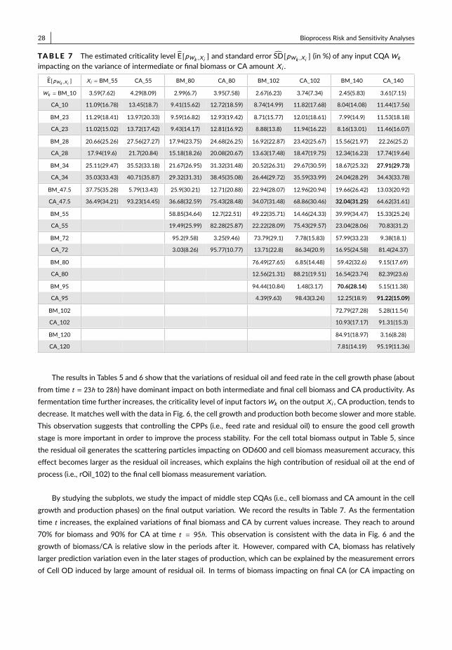
28 Bioprocess Risk and Sensitivity Analyses
TABLE 7 The estimated criticality level E[pWk ,Xi ] and standard error SD[pWk ,Xi ] (in %) of any input CQAWk
impacting on the variance of intermediate or final biomass or CA amount Xi .
E[pWk ,Xi ] Xi = BM_55 CA_55 BM_80 CA_80 BM_102 CA_102 BM_140 CA_140
Wk = BM_10 3.59(7.62) 4.29(8.09) 2.99(6.7) 3.95(7.58) 2.67(6.23) 3.74(7.34) 2.45(5.83) 3.61(7.15)
CA_10 11.09(16.78) 13.45(18.7) 9.41(15.62) 12.72(18.59) 8.74(14.99) 11.82(17.68) 8.04(14.08) 11.44(17.56)
BM_23 11.29(18.41) 13.97(20.33) 9.59(16.82) 12.93(19.42) 8.71(15.77) 12.01(18.61) 7.99(14.9) 11.53(18.18)
CA_23 11.02(15.02) 13.72(17.42) 9.43(14.17) 12.81(16.92) 8.88(13.8) 11.94(16.22) 8.16(13.01) 11.46(16.07)
BM_28 20.66(25.26) 27.56(27.27) 17.94(23.75) 24.68(26.25) 16.92(22.87) 23.42(25.67) 15.56(21.97) 22.26(25.2)
CA_28 17.94(19.6) 21.7(20.84) 15.18(18.26) 20.08(20.67) 13.63(17.48) 18.47(19.75) 12.34(16.23) 17.74(19.64)
BM_34 25.11(29.47) 35.52(33.18) 21.67(26.95) 31.32(31.48) 20.52(26.31) 29.67(30.59) 18.67(25.32) 27.91(29.73)
CA_34 35.03(33.43) 40.71(35.87) 29.32(31.31) 38.45(35.08) 26.44(29.72) 35.59(33.99) 24.04(28.29) 34.43(33.78)
BM_47.5 37.75(35.28) 5.79(13.43) 25.9(30.21) 12.71(20.88) 22.94(28.07) 12.96(20.94) 19.66(26.42) 13.03(20.92)
CA_47.5 36.49(34.21) 93.23(14.45) 36.68(32.59) 75.43(28.48) 34.07(31.48) 68.86(30.46) 32.04(31.25) 64.62(31.61)
BM_55 58.85(34.64) 12.7(22.51) 49.22(35.71) 14.46(24.33) 39.99(34.47) 15.33(25.24)
CA_55 19.49(25.99) 82.28(25.87) 22.22(28.09) 75.43(29.57) 23.04(28.06) 70.83(31.2)
BM_72 95.2(9.58) 3.25(9.46) 73.79(29.1) 7.78(15.83) 57.99(33.23) 9.38(18.1)
CA_72 3.03(8.26) 95.77(10.77) 13.71(22.8) 86.34(20.9) 16.95(24.58) 81.4(24.37)
BM_80 76.49(27.65) 6.85(14.48) 59.42(32.6) 9.15(17.69)
CA_80 12.56(21.31) 88.21(19.51) 16.54(23.74) 82.39(23.6)
BM_95 94.44(10.84) 1.48(3.17) 70.6(28.14) 5.15(11.38)
CA_95 4.39(9.63) 98.43(3.24) 12.25(18.9) 91.22(15.09)
BM_102 72.79(27.28) 5.28(11.54)
CA_102 10.93(17.17) 91.31(15.3)
BM_120 84.91(18.97) 3.16(8.28)
CA_120 7.81(14.19) 95.19(11.36)
The results in Tables 5 and 6 show that the variations of residual oil and feed rate in the cell growth phase (aboutfrom time t = 23h to 28h) have dominant impact on both intermediate and final cell biomass and CA productivity. Asfermentation time further increases, the criticality level of input factorsWk on the output Xi , CA production, tends todecrease. It matches well with the data in Fig. 6, the cell growth and production both become slower and more stable.This observation suggests that controlling the CPPs (i.e., feed rate and residual oil) to ensure the good cell growthstage is more important in order to improve the process stability. For the cell total biomass output in Table 5, sincethe residual oil generates the scattering particles impacting on OD600 and cell biomass measurement accuracy, thiseffect becomes larger as the residual oil increases, which explains the high contribution of residual oil at the end ofprocess (i.e., rOil_102) to the final cell biomass measurement variation.
By studying the subplots, we study the impact of middle step CQAs (i.e., cell biomass and CA amount in the cellgrowth and production phases) on the final output variation. We record the results in Table 7. As the fermentationtime t increases, the explained variations of final biomass and CA by current values increase. They reach to around70% for biomass and 90% for CA at time t = 95h. This observation is consistent with the data in Fig. 6 and thegrowth of biomass/CA is relative slow in the periods after it. However, compared with CA, biomass has relativelylarger prediction variation even in the later stages of production, which can be explained by the measurement errorsof Cell OD induced by large amount of residual oil. In terms of biomass impacting on final CA (or CA impacting on

Bioprocess Risk and Sensitivity Analyses 29
biomass), themost critical part is biomass at time t = 34h (or CA amount at t = 47.5h). Since cell growth needs nitrogen,the production phase usually starts when nitrogen concentration becomes small. During those periods (around 30hto 50h), nitrogen from the initial medium is consumed and both intracellular lipid (which becomes part of biomass)accumulation and extracellular CA production are induced by nitrogen limitation. It can be also observed in Fig. 6,where the sudden increase of CA total slopes happens around 30h to 50h, whose variations have critical contributionto final CA output uncertainty.
We also conduct the sensitivity analysis studying the impact of model uncertainty on the CPPs/CQAs criticalityassessment. Herewe focus on criticality assessment estimation of prOi l _28,CA_140 and prOi l _102,BM _140, which have highcriticality and overall model uncertainty; see Tables 5 and 6. The model coefficients contributing to the estimation ofprOi l _28,CA_140 include v 2rOi l _28 and 32 linear coefficients βββ on the paths from node rOi l _28 to node CA_140, whereascoefficients contributing to the estimation of pF eed_23,CA_140 include v 2F eed_23 and 36 linear coefficients βββ . We presentthe top five coefficients contributors to the estimation uncertainty of criticality prOi l _28,CA_140 and pF eed_23,CA_140, andaggregate the results for remaining coefficients in Table 8. From the results, the estimation uncertainty of variancecoefficients of CPPs (v 2
rOi l _28 and v2F eed_23) have the largest contribution to the estimation uncertainty of the criticality
prOi l _28,CA_140 and pF eed_23,CA_140. The estimation uncertainty of coefficients βββ in both sets θθθ (rOi l _28,CA_140) andθθθ (F eed_23,CA_140) have similar and relative lower contributions.
TABLE 8 The estimated relative contribution of each BN parameter estimation uncertainty (in terms of %) oncriticality assessment EPθ` (pWk ,Xi ) for pF eed_20,CA_140.
θ` ∈ θθθ (rOi l _28,CA_140) v 2rOi l _28 βCA_72,BM _80 βCA_55,CA_72 βrOi l _28,CA_34 βCA_120,CA_140 rest
EPθ` (prOi l _28,CA_140) 23.38 4.00 4.00 3.86 3.55 61.21
θ` ∈ θθθ (F eed_23,CA_140) v 2F eed_23 βBM _72,BM _80 βCA_72,BM _80 βBM _95,CA_102 βBM _72,CA_80 rest
EPθ` (pF eed_23,CA_140) 19.52 5.10 4.10 3.97 3.95 63.36
8 | CONCLUSIONS
Driven by the critical challenges in biomanufacturing, we create an integrated bioprocess knowledge graph and pro-pose interpretable risk and sensitivity analyses, which can provide the production process risk- and science-basedunderstanding, guide the CPPs/CQAs specifications and production stability control, and facilitate the process devel-opment. Since hundreds of factors can impact on the product quality and productivity, and also the amount of processobservations is often very limited, we explore the process interactions and causal relationships, and then develop aBayesian network (BN) based probabilistic knowledge graph characterizing the causal interdependencies of produc-tion process CPPs/CQAs. Building on the knowledge graph, we propose the BN-SV based sensitivity analysis to assessthe criticality of each random input factor on the variance of intermediate/final product quality attributes by usingthe Shapley value (SV), which can correctly account for input interdependencies and process structural interactions.We further introduce the BN-SV-MU sensitivity analysis, which can provide the comprehensive understanding onhow the estimation uncertainty of each part of process model coefficients impacts on the production risk analysis andCPPs/CQAs criticality assessment. It can guide bioprocess sensor monitoring and “most informative" data collectionto facilitate bioprocess learning and model uncertainty reduction. Both simulation and real case studies are used todemonstrate the promising performance of proposed bioprocess risk and sensitivity analyses.

30 Bioprocess Risk and Sensitivity Analyses
ACKNOWLEDGEMENTS
The authors are grateful for constructive comments from Dr. Barry Nelson (Northeastern University), Peter Baker(Green Mountain Quality Assurance, LLC), help from Hua Zheng (NEU) on the development of bioprocess knowledgegraph visualization, and help from Na Liu (UMass Lowell) conducting lab experiments.
referencesAyech, N., Chakour, C., andHARKAT,M.-F. (2012). New adaptivemovingwindowpca for processmonitoring. IFACProceedings
Volumes, 45(20):606–611.
Borchert, D., Suarez-Zuluaga, D. A., Sagmeister, P., Thomassen, Y. E., and Herwig, C. (2019). Comparison of data scienceworkflows for root cause analysis of bioprocesses. Bioprocess and biosystems engineering, 42(2):245–256.
Borgonovo, E. and Plischke, E. (2016). Sensitivity analysis: a review of recent advances. European Journal of OperationalResearch, 248(3):869–887.
Castillo, E., Gutiérrez, J. M., and Hadi, A. S. (1997). Sensitivity analysis in discrete bayesian networks. IEEE Transactions onSystems, Man, and Cybernetics-Part A: Systems and Humans, 27(4):412–423.
Castro, J., Gómez, D., and Tejada, J. (2009). Polynomial calculation of the shapley value based on sampling. Computers &Operations Research, 36(5):1726–1730.
Coleman, M. C. and Block, D. E. (2006). Retrospective optimization of time-dependent fermentation control strategies usingtime-independent historical data. Biotechnology and bioengineering, 95(3):412–423.
De Lira, L. d. F. B., De Vasconcelos, F. V. C., Pereira, C. F., Paim, A. P. S., Stragevitch, L., and Pimentel, M. F. (2010). Predictionof properties of diesel/biodiesel blends by infrared spectroscopy and multivariate calibration. Fuel, 89(2):405–409.
Doran, P. M. (1995). Bioprocess engineering principles. Elsevier.
Doran, P. M. (2013). Bioprocess Engineering Principles. Elsevier.
Feng, N., Wang, H. J., and Li, M. (2014). A security risk analysis model for information systems: Causal relationships of riskfactors and vulnerability propagation analysis. Information sciences, 256:57–73.
Fleischhacker, A. J. and Zhao, Y. (2011). Planning for demand failure: A dynamic lot size model for clinical trial supply chains.European Journal of Operational Research, 211(3):496–506.
Gelman, A., Carlin, J. B., Stern, H. S., and Rubin, D. B. (2004). Bayesian Data Analysis. Taylor and Francis Group, LLC, New York,2nd edition.
Guideline, I. H. T. et al. (2009). Pharmaceutical development. Q8 (R2) Current Step, 4.
Hassan, S. S., Farhan, M., Mangayil, R., Huttunen, H., and Aho, T. (2013). Bioprocess data mining using regularized regressionand random forests. BMC Systems Biology.
Helton, J. C. (1993). Uncertainty and sensitivity analysis techniques for use in performance assessment for radioactive wastedisposal. Reliability Engineering & System Safety, 42(2-3):327–367.
Kabir, G., Tesfamariam, S., Francisque, A., and Sadiq, R. (2015). Evaluating risk of water mains failure using a bayesian beliefnetwork model. European Journal of Operational Research, 240(1):220–234.
Kaminsky, P. and Wang, Y. (2015). Analytical models for biopharmaceutical operations and supply chain management: Asurvery of research literature, pharmaceutical bioprocess. Pharmaceutical Bioprocess, 2:61–73.

Bioprocess Risk and Sensitivity Analyses 31
Koller, D. and Friedman, N. (2009). Probabilistic graphical models: principles and techniques. MIT press.
Kulkarni, N. S. (2015). A modular approach for modeling active pharmaceutical ingredient manufacturing plant: a case study.In Proceedings of the 2015 Winter Simulation Conference, pages 2260–2271. IEEE Press.
Kyriakopoulos, S., Ang, K. S., Lakshmanan, M., Huang, Z., Yoon, S., Gunawan, R., and Lee, D.-Y. (2018). Kinetic modeling ofmammalian cell culture bioprocessing: The quest to advance biomanufacturing. Biotechnology Journal, 13(3):1700229.
Lakhdar, K., Savery, J., Papageorgiou, L., and Farid, S. (2007). Multiobjective long-term planning of biopharmaceutical manu-facturing facilities. Biotechnology progress, 23(6):1383–1393.
Leachman, R. C., Johnston, L., Li, S., and Shen, Z.-J. (2014). An automated planning engine for biopharmaceutical production.European Journal of Operational Research, 238(1):327–338.
Li, Y. and Yuan, J. (2006). Prediction of key state variables using support vector machines in bioprocesses. Chemical Engineering& Technology: Industrial Chemistry-Plant Equipment-Process Engineering-Biotechnology, 29(3):313–319.
Li, Y. F. and Venkatasubramanian, V. (2018). Neural network to understand process capability and process intermediatesacceptance criteria in monoclonal antibody production process. Journal of Pharmaceutical Innovation, 13(1):36–47.
Lim, A. C., Zhou, Y., Washbrook, J., Titchener-Hooker, N. J., and Farid, S. (2004). A decisional-support tool to model the impactof regulatory compliance activities in the biomanufacturing industry. Computers & chemical engineering, 28(5):727–735.
Lu, Q., Jiang, B., Gopaluni, R. B., Loewen, P. D., and Braatz, R. D. (2018). Sparse canonical variate analysis approach for processmonitoring. Journal of Process Control, 71:90–102.
Lundberg, S. M. and Lee, S.-I. (2017). A unified approach to interpreting model predictions. In Advances in neural informationprocessing systems, pages 4765–4774.
Martagan, T., Krishnamurthy, A., and Leland, P. (2018). Managing trade-offs in protein manufacturing: how much to waste?Manufacturing & Service Operations Management.
Martagan, T., Krishnamurthy, A., Leland, P. A., and Maravelias, C. T. (2017). Performance guarantees and optimal purificationdecisions for engineered proteins. Operations Research, 66(1):18–41.
Martagan, T., Krishnamurthy, A., and Maravelias, C. T. (2016). Optimal condition-based harvesting policies for biomanufactur-ing operations with failure risks. IIE Transactions, 48(5):440–461.
Mitchell, M. (2013). Determining criticality-process parameters and quality attributes part i: criticality as a continuum. Bio-Pharm International, 26(12).
Moullec, M.-L., Bouissou, M., Jankovic, M., Bocquet, J.-C., Réquillard, F., Maas, O., and Forgeot, O. (2013). Toward systemarchitecture generation and performances assessment under uncertainty using bayesian networks. Journal of MechanicalDesign, 135(4):041002.
Ojha, R., Ghadge, A., Tiwari, M. K., and Bititci, U. S. (2018). Bayesian network modelling for supply chain risk propagation.International Journal of Production Research, 56(17):5795–5819.
Otto, R., Santagostino, A., and Schrader, U. (2014). From science to operations: Questions, choices, and strategies for successin biopharma. McKinsey & Company.
Owen, A. B. (2014). Sobol’indices and shapley value. SIAM/ASA Journal on Uncertainty Quantification, 2(1):245–251.
Pharmaceutical Current Good Manufacturing Practices (CGMPs) (2004). Guidance for industry: Pat—a framework for innova-tive pharmaceutical development, manufacturing, and quality assurance. Technical report.
32 Bioprocess Risk and Sensitivity Analyses
Prinsloo, N. M., Engelbrecht, J. P., Mashapa, T. N., and Strauss, M. J. (2008). Acetone to mibk process optimization throughmultidisciplinary chemometrics and in-line nir spectroscopy. Applied Catalysis A: General, 344(1-2):20–29.
Rabitz, H. and Aliş, Ö. F. (1999). General foundations of high-dimensional model representations. Journal of MathematicalChemistry, 25(2-3):197–233.
Rader, R. A. and Langer, E. S. (2019). Single-use technologies in biopharmaceutical manufacturing: A 10-year review of trendsand the future. Single-Use Technology in Biopharmaceutical Manufacture, pages 193–200.
Rathore, A., Bhambure, R., and Ghare, V. (2010). Process analytical technology (pat) for biopharmaceutical products. Analyticaland bioanalytical chemistry, 398(1):137–154.
Severson, K., VanAntwerp, J. G., Natarajan, V., Antoniou, C., Thömmes, J., and Braatz, R. D. (2015). Elastic net with montecarlo sampling for data-based modeling in biopharmaceutical manufacturing facilities. Computers & Chemical Engineering,80:30–36.
Shapley, L. S. (1953). A value for n-person games. Contributions to the Theory of Games, 2(28):307–317.
Sobol, I. M. (1993). Sensitivity estimates for nonlinear mathematical models. Mathematical modelling and computationalexperiments, 1(4):407–414.
Sokolov, M., Morbidelli, M., Butté, A., Souquet, J., and Broly, H. (2018). Sequential multivariate cell culture modeling atmultiple scales supports systematic shaping of a monoclonal antibody toward a quality target. Biotechnology Journal,13(4):1700461.
Song, E., Nelson, B. L., and Staum, J. (2016). Shapley effects for global sensitivity analysis: Theory and computation. SIAM/ASAJournal on Uncertainty Quantification, 4(1):1060–1083.
Steinwandter, V., Borchert, D., and Herwig, C. (2019). Data science tools and applications on the way to pharma 4.0. Drugdiscovery today, 24(9):1795–1805.
Telenko, C. and Seepersad, C. C. (2014). Probabilistic graphical modeling of use stage energy consumption: a lightweightvehicle example. Journal of Mechanical Design, 136(10):101403.
Troyanskaya, O. G., Dolinski, K., Owen, A. B., Altman, R. B., and Botstein, D. (2003). A bayesian framework for combining het-erogeneous data sources for gene function prediction (in saccharomyces cerevisiae). Proceedings of the National Academyof Sciences, 100(14):8348–8353.
Van der Gaag, L. C., Renooij, S., and Coupé, V. M. (2007). Sensitivity analysis of probabilistic networks. In Advances inprobabilistic graphical models, pages 103–124. Springer.
Wagner, H. M. (1995). Global sensitivity analysis. Operations Research, 43(6):948–969.
Walsh, G. (2013). Pharmaceutical biotechnology: concepts and applications. John Wiley & Sons.
Wang, Y., Blache, R., Zheng, P., and Xu, X. (2018). A knowledge management system to support design for additive manufac-turing using bayesian networks. Journal of Mechanical Design, 140(5):051701.
Wechselberger, P., Sagmeister, P., Engelking, H., Schmidt, T., Wenger, J., and Herwig, C. (2012). Efficient feeding profileoptimization for recombinant protein production using physiological information. Bioprocess and biosystems engineering,35(9):1637–1649.
Zhai, Q., Yang, J., Xie, M., and Zhao, Y. (2014). Generalized moment-independent importance measures based on minkowskidistance. European Journal of Operational Research, 239(2):449–455.
Zi, Z. (2011). Sensitivity analysis approaches applied to systems biology models. The Institution of Engineering and Technology,5:336–346.
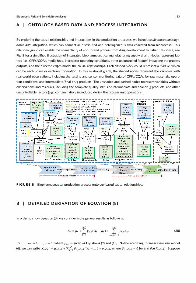
Bioprocess Risk and Sensitivity Analyses 33
A | ONTOLOGY BASED DATA AND PROCESS INTEGRATION
By exploring the causal relationships and interactions in the production processes, we introduce bioprocess ontology-based data integration, which can connect all distributed and heterogeneous data collected from bioprocess. Thisrelational graph can enable the connectivity of end-to-end process from drug development to patient response; seeFig. 8 for a simplified illustration of integrated biopharmaceutical manufacturing supply chain. Nodes represent fac-tors (i.e., CPPs/CQAs, media feed, bioreactor operating conditions, other uncontrolled factors) impacting the processoutputs, and the directed edges model the causal relationships. Each dashed block could represent a module, whichcan be each phase or each unit operation. In this relational graph, the shaded nodes represent the variables withreal-world observations, including the testing and sensor monitoring data of CPPs/CQAs for raw materials, opera-tion conditions, and intermediate/final drug products. The unshaded and dashed nodes represent variables withoutobservations and residuals, including the complete quality status of intermediate and final drug products, and otheruncontrollable factors (e.g., contamination) introduced during the process unit operations.
F IGURE 8 Biopharmaceutical production process ontology based causal relationships.
B | DETAILED DERIVATION OF EQUATION (8)
In order to show Equation (8), we consider more general results as following,
Xn = µn +mp∑k=1
γk ,n (Xk − µk ) +n∑
k=mp+1
γk ,nek , (28)
for n = mp + 1, . . . ,m + 1, where γk ,n is given as Equations (9) and (10). Notice according to linear Gaussian model(6), we can write Xmp+1 = µmp+1 +
∑mp
k=1 βk ,mp+1 (Xk − µk ) + emp+1, where βk ,mp+1 = 0 for k < P a (Xmp+1) . Suppose
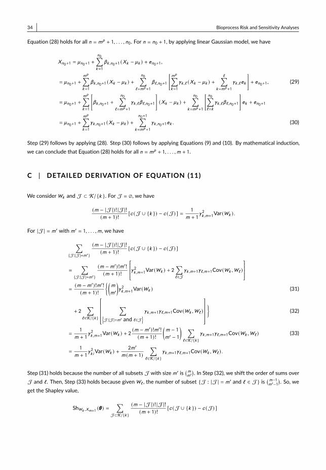
34 Bioprocess Risk and Sensitivity Analyses
Equation (28) holds for all n = mp + 1, . . . , n0. For n = n0 + 1, by applying linear Gaussian model, we have
Xn0+1 = µn0+1 +
n0∑k=1
βk ,n0+1 (Xk − µk ) + en0+1,
= µn0+1 +mp∑k=1
βk ,n0+1 (Xk − µk ) +n0∑
`=mp+1
β` ,n0+1
[mp∑k=1
γk ,` (Xk − µk ) +∑
k=mp+1
γk ,` ek
]+ en0+1, (29)
= µn0+1 +mp∑k=1
[βk ,n0+1 +
n0∑`=mp+1
γk ,`β` ,n0+1
](Xk − µk ) +
n0∑k=mp+1
[ n0∑`=k
γk ,`β` ,n0+1
]ek + en0+1
= µn0+1 +mp∑k=1
γk ,n0+1 (Xk − µk ) +n0+1∑
k=mp+1
γk ,n0+1ek . (30)
Step (29) follows by applying (28). Step (30) follows by applying Equations (9) and (10). By mathematical induction,we can conclude that Equation (28) holds for all n = mp + 1, . . . ,m + 1.
C | DETAILED DERIVATION OF EQUATION (11)
We considerWk and J ⊂ K/{k }. For J = ∅, we have
(m − |J |)! |J |!(m + 1)! [c (J ∪ {k }) − c (J) ] = 1
m + 1γ2k ,m+1Var(Wk ) .
For |J | = m′ with m′ = 1, . . . ,m , we have
∑{J:|J|=m′}
(m − |J |)! |J |!(m + 1)! [c (J ∪ {k }) − c (J) ]
=∑
{J:|J|=m′}
(m −m′)!m′!(m + 1)!
γ2k ,m+1Var(Wk ) + 2∑`∈J
γk ,m+1γ` ,m+1Cov(Wk ,W` )
=(m −m′)!m′!(m + 1)!
{(m
m′
)γ2k ,m+1Var(Wk ) (31)
+ 2∑
`∈K/{k }
∑
{J:|J|=m′ and `∈J
} γk ,m+1γ` ,m+1Cov(Wk ,W` )
}
(32)
=1
m + 1γ2k ,m+1Var(Wk ) + 2
(m −m′)!m′!(m + 1)!
(m − 1m′ − 1
) ∑`∈K/{k }
γk ,m+1γ` ,m+1Cov(Wk ,W` ) (33)
=1
m + 1γ2k iVar(Wk ) +
2m′
m (m + 1)∑
`∈K/{k }γk ,m+1γ` ,m+1Cov(Wk ,W` ) .
Step (31) holds because the number of all subsets J with size m′ is(mm′
). In Step (32), we shift the order of sums over
J and ` . Then, Step (33) holds because givenW` , the number of subset {J : |J | = m′ and ` ∈ J} is(m−1m′−1
). So, we
get the Shapley value,
ShWk ,Xm+1 (θθθ) =∑
J⊂K/{k }
(m − |J |)! |J |!(m + 1)! [c (J ∪ {k }) − c (J) ]
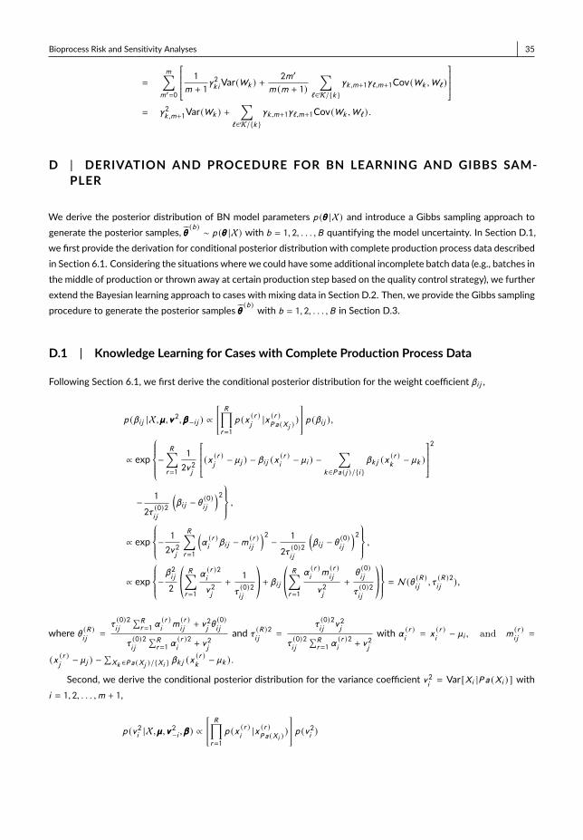
Bioprocess Risk and Sensitivity Analyses 35
=m∑
m′=0
1
m + 1γ2k iVar(Wk ) +
2m′
m (m + 1)∑
`∈K/{k }γk ,m+1γ` ,m+1Cov(Wk ,W` )
= γ2k ,m+1Var(Wk ) +
∑`∈K/{k }
γk ,m+1γ` ,m+1Cov(Wk ,W` ) .
D | DERIVATION AND PROCEDURE FOR BN LEARNING AND GIBBS SAM-PLER
We derive the posterior distribution of BN model parameters p (θθθ |X) and introduce a Gibbs sampling approach togenerate the posterior samples, θθθ (b ) ∼ p (θθθ |X) with b = 1, 2, . . . ,B quantifying the model uncertainty. In Section D.1,we first provide the derivation for conditional posterior distribution with complete production process data describedin Section 6.1. Considering the situations where we could have some additional incomplete batch data (e.g., batches inthe middle of production or thrown away at certain production step based on the quality control strategy), we furtherextend the Bayesian learning approach to cases with mixing data in Section D.2. Then, we provide the Gibbs samplingprocedure to generate the posterior samples θθθ (b ) with b = 1, 2, . . . ,B in Section D.3.
D.1 | Knowledge Learning for Cases with Complete Production Process Data
Following Section 6.1, we first derive the conditional posterior distribution for the weight coefficient βi j ,
p (βi j |X,µµµ,vvv 2,βββ−i j ) ∝[R∏r=1
p (x (r )j|x (r )P a (Xj )
)]p (βi j ),
∝ exp
−R∑r=1
1
2v 2j
(x (r )j − µj ) − βi j (x (r )i − µi ) −∑
k ∈P a (j )/{i }βk j (x (r )k − µk )
2
− 1
2τ (0)2i j
(βi j − θ (0)i j
)2 ,∝ exp
−1
2v 2j
R∑r=1
(α(r )iβi j −m (r )i j
)2− 1
2τ (0)2i j
(βi j − θ (0)i j
)2 ,∝ exp
−β 2i j
2©«R∑r=1
α(r )2i
v 2j
+1
τ(0)2i j
ª®¬ + βi j ©«R∑r=1
α(r )im(r )i j
v 2j
+θ(0)i j
τ(0)2i j
ª®¬ = N(θ (R )i j
, τ(R )2i j),
where θ (R )i j
=τ(0)2i j
∑Rr=1 α
(r )im(r )i j
+ v 2jθ(0)i j
τ(0)2i j
∑Rr=1 α
(r )2i
+ v 2j
and τ (R )2i j
=τ(0)2i j
v 2j
τ(0)2i j
∑Rr=1 α
(r )2i
+ v 2j
with α (r )i
= x(r )i− µi , and m
(r )i j
=
(x (r )j− µj ) −
∑Xk ∈P a (Xj )/{Xi } βk j (x
(r )k− µk ) .
Second, we derive the conditional posterior distribution for the variance coefficient v 2i= Var[Xi |P a (Xi ) ] with
i = 1, 2, . . . ,m + 1,
p (v 2i |X,µµµ,vvv2−i ,βββ ) ∝
[R∏r=1
p (x (r )i|x (r )P a (Xi )
)]p (v 2i )

36 Bioprocess Risk and Sensitivity Analyses
∝ (v 2i )−R/2−κ (0)
i/2−1 exp
−1
2v 2j
R∑r=1
(x (r )i − µi ) −∑
Xk ∈P a (Xi )βk i (x (r )k − µk )
2
∝ (v 2i )−R/2−κ (0)
i/2−1 exp
{− 1
2v 2j
R∑r=1
u(r )2i−λ(0)i
2v 2j
}= Inv-Γ
(κ(R )i
2,λ(R )i
2
),
where κ (R )i
= κ (0)i
+ R , λ (R )i
= λ (0)i
+∑Rr=1 u
(r )2i
and u (r )i
= (x (r )i− µi ) −
∑Xk ∈P a (Xi ) βk i (x
(r )k− µk ) .
Third, we derive the conditional posterior distribution of mean coefficient µi with i = 1, 2, . . . ,m + 1 for any CPPand CQA,
p (µi |X,µµµ−i ,vvv 2,βββ ) ∝ p (µi )R∏r=1
p (x (r )i |x (r )P a (Xi ) )∏
j ∈S(Xi )p (x (r )
j|x (r )P a (Xj )
)
∝ exp{− 1
2v 2i
R∑r=1
(x (r )i − µi ) −∑
Xk ∈P a (Xi )βk i (x (r )k − µk )
2
−R∑r=1
∑Xj ∈S(Xi )
1
2v 2j
(x (r )j − µj ) −∑
Xk ∈P a (Xj )βk j (x (r )k − µk )
2
− 1
2σ (0)2i
(µi − µ (0)i
)2 },
∝ exp−
1
2v 2i
R∑r=1
(µi − a (r )i
)2−
R∑r=1
∑Xj ∈S(Xi )
− 1
2v 2j
(βi j µi − c (r )i j
)2− 1
2σ (0)2i
(µi − µ (0)i
)2},
∝ exp−µ2i
2©« Rv 2i +
∑Xj ∈S (Xi )
Rβ 2i j
v 2j
+1
σ(0)2i
ª®¬ + µi ©«R∑r=1
a(r )i
v 2i
+R∑r=1
∑Xj ∈S(Xi )
βi j c(r )i j
v 2j
+µ(0)i
σ(0)2i
)}= N(µ (R )
i,σ(R )2i),
where µ (R )i
= σ(R )2i
µ(0)i
σ(0)2i
+∑Rr=1
a(r )i
v 2i
+∑Rr=1
∑Xj ∈S (Xi )
βi j c(r )i j
v 2j
and 1
σ(R )2i
=1
σ(0)2i
+R
v 2i
+∑Xj ∈S (Xi )
Rβ 2i j
v 2j
, with
a(r )i
= x (r )i−∑
Xk ∈P a (Xi ) βk j (x(r )k− µk ) and c (r )i j = βi j x
(r )i− (x (r )
j− µj ) +
∑Xk ∈P a (Xj )/{Xi } βk j (x
(r )k− µk ) .
D.2 | Knowledge Learning for Cases with Mixing Data
Except the case with complete production data discussed in Section D.1, we consider the cases with additional incom-plete data corresponding to certain “Top Sub-Graph", denoted by G (N′ |θθθ (N′)) with N′ ⊆ N, such that any CQA nodeXj ∈ N′ has P a (Xj ) ⊂ N′. Since batch data collected from biopharmaceutical production process are usually limited,we want to fully utilize both complete and incomplete data to estimate the BN model coefficients and improve ourknowledge of production process.
Without loss of generality, we consider the real-world data including two data sets X = {X1, X2 } with the com-plete data X1 = {(x (r1 )1 , x
(r1 )2 , . . . , x
(r1 )m+1) for r1 = 1, 2, . . . , R1 } and the incomplete data X2 = {(x (r2 )i
: Xi ∈ N′) forr2 = R1 + 1, R1 + 2, . . . , R }, where R = R1 + R2. Our approach can be easily extended to cases with multiple in-

Bioprocess Risk and Sensitivity Analyses 37
complete data sets. We use the same prior distribution p (µµµ,vvv 2,βββ ) as shown in Equation (13). Given the mixing dataX = {X1, X2 }, we can derive the posterior distribution of θθθ,
p (µµµ,vvv 2,βββ |X) ∝R1∏r1=1
[m+1∏i=1
p (x (r1 )i|x (r1 )P a (Xi )
)]
R∏r2=R1+1
∏Xi ∈N′
p (x (r2 )i|x (r2 )P a (Xi )
) p (µµµ,vvv 2,βββ ) .
For βi j with Xj < N′ or v 2i and µi with node Xi < N′, the conditional posterior is the same as complete data case andwe can utilize Equations (15), (16) and (17) by replacing X with X1.
Thus, to derive the full Gibbs sampler, we only need to provide the updated conditional posterior accounting forthose nodes included in the incomplete data set X2. We first derive the conditional posterior distribution for weightcoefficient βi j with Xj ∈ N′.
p (βi j |X,µµµ,vvv 2,βββ−i j ) ∝R1+R2∏r=1
p (x (r )j|x (r )P a (Xj )
) p (βi j ),
∝ exp
−R1+R2∑r=1
1
2v 2j
(x (r )j − µj ) − βi j (x (r )i − µi ) −∑
k ∈P a (j )/{i }βk j (x (r )k − µk )
2
− 1
2τ (0)2i j
(βi j − θ (0)i j
)2 ,∝ exp
−1
2v 2j
R1+R2∑r=1
(α(r )iβi j −m (r )i j
)2− 1
2τ (0)2i j
(βi j − θ (0)i j
)2 ,∝ exp
−β 2i j
2©«R1+R2∑r=1
α(r )2i
v 2j
+1
τ(0)2i j
ª®¬ + βi j ©«R1+R2∑r=1
α(r )im(r )i j
v 2j
+θ(0)i j
τ(0)2i j
ª®¬
= N(θ (R1+R2 )i j
, τ(R1+R2 )2i j
), (34)
where θ (R1+R2 )i j
=τ(0)2i j
∑R1+R2r=1 α
(r )im(r )i j
+ v 2jθ(0)i j
τ(0)2i j
∑R1+R2r=1 α
(r )2i
+ v 2j
and τ (R1+R2 )2i j
=τ(0)2i j
v 2j
τ(0)2i j
∑R1+R2r=1 α
(r )2i
+ v 2j
with α (r )i
= x (r )i− µi and
m(r )i j
= (x (r )j− µj ) −
∑Xk ∈P a (Xj )/{Xi } βk j (x
(r )k− µk ) for r = 1, 2, . . . , R .
Then, we derive the conditional posterior distribution for v 2iwith Xi ∈ N′,
p (v 2i |X,µµµ,vvv2−i ,βββ ) ∝
R1+R2∏r=1
p (x (r )i|x (r )P a (Xi )
) p (v 2i ),
∝ (v 2i )−(R1+R2 )/2−κ
(0)i/2−1 exp
−1
2v 2j
R1+R2∑r=1
(x (r )i − µi ) −∑
Xk ∈P a (Xi )βk i (x (r )k − µk )
2 ,
∝ (v 2i )−(R1+R2 )/2−κ
(0)i/2−1 exp
− 1
2v 2j
R1+R2∑r=1
u(r )2i−λ(0)i
2v 2j
= Inv-Γ ©«
κ(R1+R2 )i
2,λ(R1+R2 )i
2ª®¬ , (35)
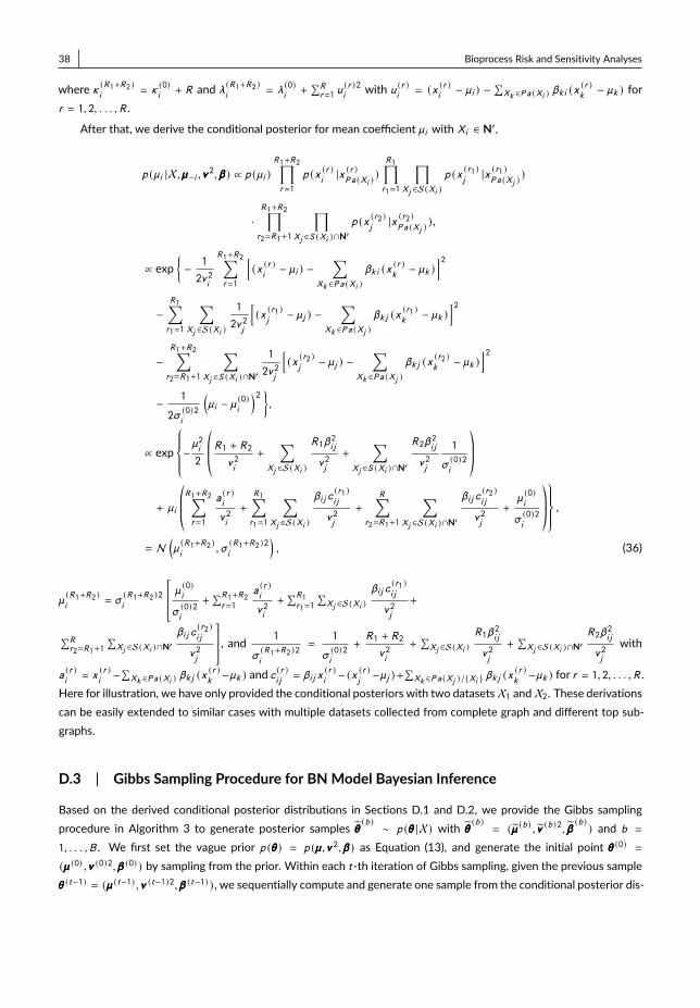
38 Bioprocess Risk and Sensitivity Analyses
where κ (R1+R2 )i
= κ(0)i
+ R and λ (R1+R2 )i
= λ (0)i
+∑Rr=1 u
(r )2i
with u (r )i
= (x (r )i− µi ) −
∑Xk ∈P a (Xi ) βk i (x
(r )k− µk ) for
r = 1, 2, . . . , R .
After that, we derive the conditional posterior for mean coefficient µi with Xi ∈ N′,
p (µi |X,µµµ−i ,vvv 2,βββ ) ∝ p (µi )R1+R2∏r=1
p (x (r )i|x (r )P a (Xi )
)R1∏r1=1
∏Xj ∈S(Xi )
p (x (r1 )j|x (r1 )P a (Xj )
)
·R1+R2∏r2=R1+1
∏Xj ∈S (Xi )∩N′
p (x (r2 )j|x (r2 )P a (Xj )
),
∝ exp{− 1
2v 2i
R1+R2∑r=1
[(x (r )i− µi ) −
∑Xk ∈P a (Xi )
βk i (x (r )k − µk )]2
−R1∑r1=1
∑Xj ∈S(Xi )
1
2v 2j
[(x (r1 )j− µj ) −
∑Xk ∈P a (Xj )
βk j (x(r1 )k− µk )
]2−
R1+R2∑r2=R1+1
∑Xj ∈S (Xi )∩N′
1
2v 2j
[(x (r2 )j− µj ) −
∑Xk ∈P a (Xj )
βk j (x(r2 )k− µk )
]2− 1
2σ (0)2i
(µi − µ (0)i
)2 },
∝ exp
−µ2i
2
©«R1 + R2
v 2i
+∑
Xj ∈S(Xi )
R1β2i j
v 2j
+∑
Xj ∈S (Xi )∩N′
R2β2i j
v 2j
1
σ(0)2i
ª®®¬+ µi
©«R1+R2∑r=1
a(r )i
v 2i
+
R1∑r1=1
∑Xj ∈S(Xi )
βi j c(r1 )i j
v 2j
+R∑
r2=R1+1
∑Xj ∈S(Xi )∩N′
βi j c(r2 )i j
v 2j
+µ(0)i
σ(0)2i
ª®®¬ ,
= N(µ(R1+R2 )i
,σ(R1+R2 )2i
), (36)
µ(R1+R2 )i
= σ(R1+R2 )2i
µ(0)i
σ(0)2i
+∑R1+R2r=1
a(r )i
v 2i
+∑R1r1=1
∑Xj ∈S(Xi )
βi j c(r1 )i j
v 2j
+
∑Rr2=R1+1
∑Xj ∈S(Xi )∩N′
βi j c(r2 )i j
v 2j
, and1
σ(R1+R2 )2i
=1
σ(0)2i
+R1 + R2
v 2i
+∑Xj ∈S(Xi )
R1β2i j
v 2j
+∑Xj ∈S(Xi )∩N′
R2β2i j
v 2j
with
a(r )i
= x (r )i−∑Xk ∈P a (Xi ) βk j (x
(r )k−µk ) and c (r )i j = βi j x
(r )i−(x (r )
j−µj )+
∑Xk ∈P a (Xj )/{Xi } βk j (x
(r )k−µk ) for r = 1, 2, . . . , R .
Here for illustration, we have only provided the conditional posteriors with two datasets X1 and X2. These derivationscan be easily extended to similar cases with multiple datasets collected from complete graph and different top sub-graphs.
D.3 | Gibbs Sampling Procedure for BN Model Bayesian Inference
Based on the derived conditional posterior distributions in Sections D.1 and D.2, we provide the Gibbs samplingprocedure in Algorithm 3 to generate posterior samples θθθ (b ) ∼ p (θθθ |X) with θθθ (b ) = (µµµ (b ) , vvv (b )2, βββ (b ) ) and b =
1, . . . ,B . We first set the vague prior p (θθθ) = p (µµµ,vvv 2,βββ ) as Equation (13), and generate the initial point θθθ (0) =(µµµ (0) ,vvv (0)2,βββ (0) ) by sampling from the prior. Within each t -th iteration of Gibbs sampling, given the previous sampleθθθ (t−1) = (µµµ (t−1) ,vvv (t−1)2,βββ (t−1) ) , we sequentially compute and generate one sample from the conditional posterior dis-
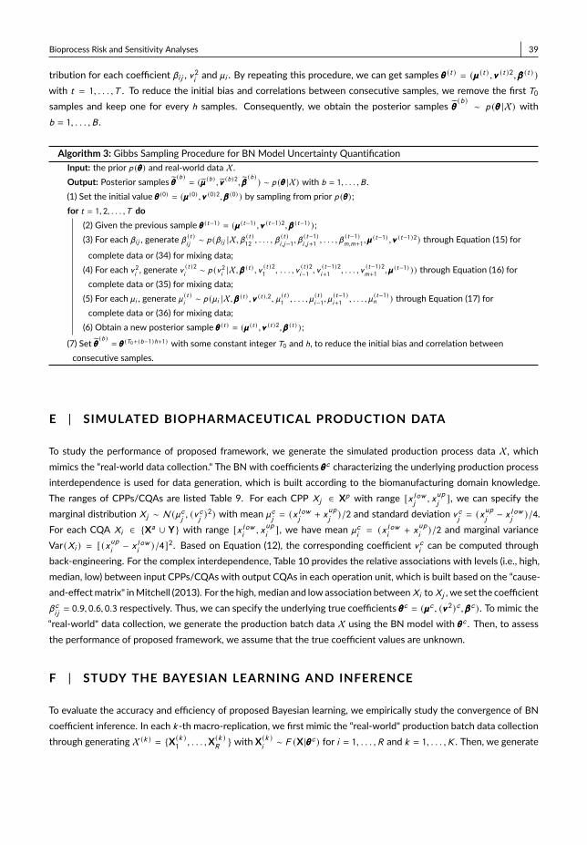
Bioprocess Risk and Sensitivity Analyses 39
tribution for each coefficient βi j , v 2i and µi . By repeating this procedure, we can get samples θθθ (t ) = (µµµ (t ) ,vvv (t )2,βββ (t ) )with t = 1, . . . ,T . To reduce the initial bias and correlations between consecutive samples, we remove the first T0samples and keep one for every h samples. Consequently, we obtain the posterior samples θθθ (b ) ∼ p (θθθ |X) withb = 1, . . . ,B .
Algorithm 3: Gibbs Sampling Procedure for BN Model Uncertainty QuantificationInput: the prior p (θθθ) and real-world data X.Output: Posterior samples θθθ (b ) = (µµµ (b ) , vvv (b )2, βββ (b ) ) ∼ p (θθθ |X) with b = 1, . . . ,B .(1) Set the initial value θθθ (0) = (µµµ (0) ,vvv (0)2,βββ (0) ) by sampling from prior p (θθθ) ;for t = 1, 2, . . . ,T do
(2) Given the previous sample θθθ (t−1) = (µµµ (t−1) ,vvv (t−1)2,βββ (t−1) ) ;(3) For each βi j , generate β (t )i j ∼ p (βi j |X, β
(t )12 , . . . , β
(t )i ,j−1, β
(t−1)i ,j+1 , . . . , β
(t−1)m,m+1,µµµ
(t−1) ,vvv (t−1)2) through Equation (15) for
complete data or (34) for mixing data;(4) For each v 2i , generate v
(t )2i∼ p (v 2i |X,βββ
(t ) ,v (t )21 , . . . ,v(t )2i−1 ,v
(t−1)2i+1 , . . . ,v
(t−1)2m+1 ,µµµ
(t−1) )) through Equation (16) forcomplete data or (35) for mixing data;
(5) For each µi , generate µ (t )i ∼ p (µi |X,βββ(t ) ,vvv (t ) ,2, µ (t )1 , . . . , µ
(t )i−1, µ
(t−1)i+1 , . . . , µ
(t−1)n ) through Equation (17) for
complete data or (36) for mixing data;(6) Obtain a new posterior sample θθθ (t ) = (µµµ (t ) ,vvv (t )2,βββ (t ) ) ;
(7) Set θθθ (b ) = θθθ (T0+(b−1)h+1) with some constant integerT0 and h, to reduce the initial bias and correlation betweenconsecutive samples.
E | SIMULATED BIOPHARMACEUTICAL PRODUCTION DATA
To study the performance of proposed framework, we generate the simulated production process data X, whichmimics the “real-world data collection." The BN with coefficients θθθc characterizing the underlying production processinterdependence is used for data generation, which is built according to the biomanufacturing domain knowledge.The ranges of CPPs/CQAs are listed Table 9. For each CPP Xj ∈ Xp with range [x l ow
j, xupj], we can specify the
marginal distribution Xj ∼ N(µcj , (vcj)2) with mean µc
j= (x l ow
j+ x
upj)/2 and standard deviation v c
j= (xup
j− x l ow
j)/4.
For each CQA Xi ∈ {Xa ∪ Y} with range [x l owi, xupi], we have mean µc
i= (x l ow
i+ x
upi)/2 and marginal variance
Var(Xi ) = [ (xupi − xl owi)/4]2. Based on Equation (12), the corresponding coefficient v c
ican be computed through
back-engineering. For the complex interdependence, Table 10 provides the relative associations with levels (i.e., high,median, low) between input CPPs/CQAs with output CQAs in each operation unit, which is built based on the “cause-and-effectmatrix" inMitchell (2013). For the high, median and low association betweenXi toXj , we set the coefficientβ ci j= 0.9, 0.6, 0.3 respectively. Thus, we can specify the underlying true coefficients θθθc = (µµµc , (vvv 2)c ,βββ c ) . To mimic the
“real-world" data collection, we generate the production batch data X using the BN model with θθθc . Then, to assessthe performance of proposed framework, we assume that the true coefficient values are unknown.
F | STUDY THE BAYESIAN LEARNING AND INFERENCE
To evaluate the accuracy and efficiency of proposed Bayesian learning, we empirically study the convergence of BNcoefficient inference. In each k -th macro-replication, we first mimic the “real-world" production batch data collectionthrough generating X (k ) = {X(k )1 , . . . ,X
(k )R} with X(k )
i∼ F (X |θθθc ) for i = 1, . . . , R and k = 1, . . . ,K . Then, we generate
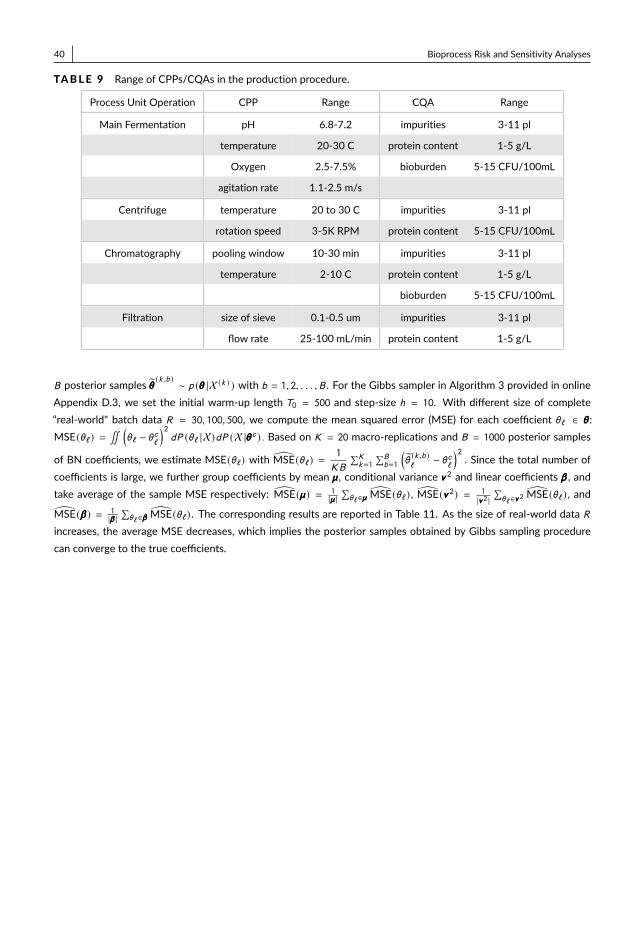
40 Bioprocess Risk and Sensitivity Analyses
TABLE 9 Range of CPPs/CQAs in the production procedure.
Process Unit Operation CPP Range CQA Range
Main Fermentation pH 6.8-7.2 impurities 3-11 pl
temperature 20-30 C protein content 1-5 g/L
Oxygen 2.5-7.5% bioburden 5-15 CFU/100mL
agitation rate 1.1-2.5 m/s
Centrifuge temperature 20 to 30 C impurities 3-11 pl
rotation speed 3-5K RPM protein content 5-15 CFU/100mL
Chromatography pooling window 10-30 min impurities 3-11 pl
temperature 2-10 C protein content 1-5 g/L
bioburden 5-15 CFU/100mL
Filtration size of sieve 0.1-0.5 um impurities 3-11 pl
flow rate 25-100 mL/min protein content 1-5 g/L
B posterior samples θθθ (k ,b ) ∼ p (θθθ |X (k ) ) with b = 1, 2, . . . ,B . For the Gibbs sampler in Algorithm 3 provided in onlineAppendix D.3, we set the initial warm-up length T0 = 500 and step-size h = 10. With different size of complete“real-world" batch data R = 30, 100, 500, we compute the mean squared error (MSE) for each coefficient θ` ∈ θθθ:MSE(θ` ) =
∬ (θ` − θc`
)2dP (θ` |X)dP (X |θθθc ) . Based on K = 20 macro-replications and B = 1000 posterior samples
of BN coefficients, we estimate MSE(θ` ) with MSE(θ` ) =1
KB
∑Kk=1
∑Bb=1
(θ(k ,b )`
− θc`
)2. Since the total number of
coefficients is large, we further group coefficients by mean µµµ, conditional variance vvv 2 and linear coefficients βββ , andtake average of the sample MSE respectively: MSE(µµµ) = 1
|µµµ |∑θ` ∈µµµ MSE(θ` ) , MSE(vvv 2) = 1
|vvv2 |∑θ` ∈vvv2 MSE(θ` ) , and
MSE(βββ ) = 1|βββ |
∑θ` ∈βββ MSE(θ` ) . The corresponding results are reported in Table 11. As the size of real-world data R
increases, the average MSE decreases, which implies the posterior samples obtained by Gibbs sampling procedurecan converge to the true coefficients.
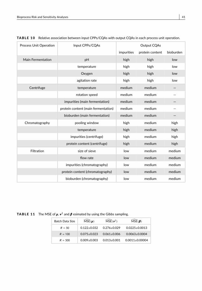
Bioprocess Risk and Sensitivity Analyses 41
TABLE 10 Relative association between input CPPs/CQAs with output CQAs in each process unit operation.
Process Unit Operation Input CPPs/CQAs Output CQAs
impurities protein content bioburden
Main Fermentation pH high high low
temperature high high low
Oxygen high high low
agitation rate high high low
Centrifuge temperature medium medium —
rotation speed medium medium —
impurities (main fermentation) medium medium —
protein content (main fermentation) medium medium —
bioburden (main fermentation) medium medium —
Chromatography pooling window high medium high
temperature high medium high
impurities (centrifuge) high medium high
protein content (centrifuge) high medium high
Filtration size of sieve low medium medium
flow rate low medium medium
impurities (chromatography) low medium medium
protein content (chromatography) low medium medium
bioburden (chromatography) low medium medium
TABLE 11 The MSE of µµµ, vvv 2 and βββ esimated by using the Gibbs sampling.
Batch Data Size MSE(µµµ) MSE(vvv 2) MSE(βββ )
R = 30 0.122±0.032 0.276±0.029 0.0225±0.0013
R = 100 0.075±0.023 0.061±0.006 0.0063±0.0004
R = 500 0.009±0.003 0.013±0.001 0.0011±0.00004