Internet Appendix for “Loan Spreads and Credit Cycles: The ...

Internet Appendix for

“Loan Spreads and Credit Cycles:

The Role of Lenders’ Personal Economic Experiences”

Daniel Carvalho, Janet Gao, and Pengfei Ma

Abstract

This appendix provides additional information and analyses that complement the main results in the paper. Section 1 provides details on our data collection process. Section 2 provides anecdotal evidence that supports the discussion in our paper on the role of the loan officers we analyze. Section 3 presents the distribution of loan officer properties and borrower headquarters across states. Section 4 examines the link between aggregate housing growth experiences of loan officers and loan spreads. In Section 5, we extend a falsification test in the paper. Sections 6 and 7 examine the robustness of our results to various geographical ranges and subsample periods. Section 8 provides additional evidence on how officer personal experiences asymmetrically affect the pricing of riskier loans. In Section 9, we show that our cross-sectional results are robust to controlling for matched officer growth by bank and region. Section 10 reports the distribution of collateral types in our sample and across all Dealscan loans. Section 11 presents evidence that borrowers’ real estate share is not associated with higher credit risk. Section 12 shows the first-stage results from our instrumental-variable analyses. Section 13 provides evidence on the connection between borrower and loan characteristics and the lead arranger share in syndicated loans. Section 14 further addresses the concern that borrower fundamentals could drive our results. Section 15 provides additional robustness checks regarding controls and sampling choices. Section 16 examines the effect of loan officer personal experiences on other, non-pricing loan terms and outcomes. Finally, Section 17 shows the robustness of our results to considering only primary residences, and to including renters.

1. Data Collection Process

We provide additional details on how we collect our data. Our initial sample identifies the names of loan officers by looking at the signatures of loan agreements (see Section 1.2). In our initial sample, we have the loan officer’s name, affiliation (bank) when they signed the loan and loan deal information from Dealscan. We then basically followed Cheng, Raina and Xiong’s (2014) online instructions to collect data from LexisNexis Public Records. We made some minor changes to their algorithms to fit our purpose and increase the data accuracy.

1.1. Procedure to Identify Target Loan Officer on LexisNexis

We first collect additional information (employment information, working location, education information, graduation year, etc.) about our sample loan officers from LinkedIn. We use a loan officer’s name and affiliation when they signed the loan contracts to search for the officer on LinkedIn to get further information like employment information, education information, location information, etc. In doing so, we require the date when our target loan officer signed a loan contract under a certain bank lies in the time period listed on LinkedIn during which the target loan officer works for the same bank. If we cannot identify a loan officer on LinkedIn, we search for information regarding his (her) career path on the internet. If the target lives outside of the U.S., we classify this loan officer’s location as “Foreign.”1

We then perform the following algorithms to identify a loan officer’s LexID on LexisNexis.

Algorithm 1. Search for a loan officer based on Name and Location/Address (if available from LinkedIn). Then filter through the possible matches based on (a) Age Range, (b) Employment Information, and (c) Education Information.

We start searching by an officer’s name and location (if available from LinkedIn) on LexisNexis. We then check manually all the search results returned on LexisNexis according to the following matching criteria:

i. “Age” on LexisNexis should be reasonably matched with the dates when the loan officer signed for loan contracts (we assume the loan officer was between 20 and 70 years old when signing for the loan contracts). Additionally, if we can find graduation year from LinkedIn, we follow the assumption used in Pool, Stoffman and Yonker (2012) that the loan officer was between 18 and 24 years old when graduating. We remove records that are not consistent with the above-listed age range. If we are able to pinpoint exactly one person on LexisNexis, we consider this as the correct match. If multiple records remain after filtering by age range, we continue to the next step.

ii. “Employment Locator” on LexisNexis should match with a loan officer’s affiliation shown on the loan contract and employment information from LinkedIn. We require a potential match on LexisNexis to have at least one employer that corresponds to the employers shown in LinkedIn and SEC contract. If we are able to pinpoint exactly one person on LexisNexis, we consider this as the correct match. If we find no match of the employer or we do not have employment information on LexisNexis, proceed to Algorithm2.

1 We search for this person without specifying “Location” on LexisNexis.

iii. “Possible Education” on LexisNexis should match with education information from LinkedIn (if education is available from both data sources). If we are able to pinpoint exactly one person on LexisNexis, we consider this as the correct match. If we find no match of the employer or we do not have employment information on LexisNexis, proceed to Algorithm2.

If we find multiple matching results following the steps above, we will search for some additional information on the internet to pinpoint the correct match. This describes Algorithm 2. If multiple records still remain after this procedure, we provide multiple matches.

Algorithm 2. Relax the criteria on Employment. Redo the search based on Name and Location. Filter through the matches by Other Information (collected from the internet).

i. Match by Education: Match “Possible Education” on LexisNexis with education information from LinkedIn (if we can get this data both from LinkedIn and LexisNexis). If we are able to pinpoint exactly one person on Nexis, we consider this a correct match.

ii. Match by Industry: Based on the “Employment Locator” on LexisNexis, check whether at least one employer is in the Banking/Finance industry. If we are able to pinpoint exactly one person on LexisNexis, we consider it as a correct match.

iii. If we find only one matched result and we do not have enough information to perform the above steps, then we consider it as a (roughly) correct match.

1.2. Procedure to Collect Property Ownership Information

We first collet all the deed transfer records, mortgage records, and tax assessment records of the properties related to all the address related to our identified loan officers from LexisNexis. We then follow the steps below to get the dates when the target gained or released control of the property. This procedure closely follows the instructions provided by Cheng, Raina and Xiong’s (2014).

A. We first identify all the people that are once listed in the deed records, mortgage records or tax assessment records together with a loan officer in our sample (these people share ownership of a property with our target loan officer). We classify these people as “associates” of the loan officer. We refer to both the loan officer and his (her) associates as a “target” in the following.

B. Find all the properties for which a target is listed as buyer or seller in at least one deed record, whose mortgage record contains a loan officer (or associates), or for which a loan officer (or associates) is listed in the tax assessment record as an owner. We identify these properties as our target properties. We then collect purchase and sale dates for these properties.

C. Get the date when the target gained control of the property. 1. Find the earliest deed record with the target listed as “Buyer”. Use this deed record to collect the

“Contract Date,” if available, or the “Recording Date” as Property Purchase Date.

2. If there is no deed record with the target listed as “Buyer”, then find the earliest mortgage record with “Mortgage Type” of “Purchase Money”. Use this mortgage record to collect the “Contract Date,” if available, or the “Recording Date” (if deed record does not already provide this information) as Property Purchase Date.

3. If we can’t get the Property Purchase Date from deed records and mortgage records, we then try to find tax assessment records for the property with the target’s name (or the name of someone associated with the target) as the “Owner”.

1) If we can find “Recording Date” in these assessment records, then collect it as Property Purchase Date.

2) If we cannot find “Recording Date” in these assessment records, then we try to find a tax assessment record for a person who owns the property after our target, Often, such records also have information on “Prior Recording Date”. We use the “Prior Recording Date” to record the Property Purchase Date for our target.

4. If we cannot find the date when the target gained control of the property, we leave it as missing.

D. Get the date when the target released control of the property. 1. Find the latest deed record for the property in which the target (and/or anyone the loan officer is

associated with) listed as “Seller”. Use the record to collect the “Contract Date” as Property Sale Date if available. If not, use the “Recording Date”.

2. If there is no deed record in which the target released control of the property, then the property is either:

Still owned by the target if:

There are no assessment/deed/mortgage records with other people as owners of the property with dates that are later than the records associated with our target. And the assessment records for the property with the target’s name come close to present-day (e.g., we have assessment records reaching until 2015 or so). Then we set Property Sale Date as 2019 (which indicates the property is still currently owned by the target).

Or sold without a deed record:

1) There are tax assessment/deed/mortgage records with other people listed as owners of the property with dates that are later than the records associated with our target; if so, then try to get the Property Sale Date by using the following two ways (If we can get the date from both, we use the earlier one):

a. Tax assessment records: find a tax assessment record for a person who owns the property after our target. Use the “Recording Date” in the assessment records to fill in the Property Sale Date.

b. Mortgage records: find a mortgage record for a person who buys the property after our target in the list with “Mortgage Type” of “Purchase Money”. Treat this record as the document capturing data on the transaction in which the next owner gains control of the property. Use this mortgage record to collect the “Contract Date,” if available, or the “Recording Date” as Property Sale Date.

2) If we can’t get the Property Sale Date by 1), and the assessment records for the property with the target’s name do not come close to present-date (e.g., the last record at all for the property is in 2010 or before). Then set the Property Sale Date as missing.

3. If we can’t find the date when the target released control of the property, we leave it as missing. E. If we cannot get the purchase and/or sale date for the property. We use the earliest tax assessment

record year for the purchase date and/or the latest tax assessment record year for the sale date. The idea is that even though we do not know when our target loan officer bought or sold this property, but we are sure that during this time period, our target loan officer has the ownership for this property.

1.3. Identifying Primary Residence and Rental Property

In our final sample, there are officers who own multiple properties at the time of loan origination. In order to identify their primary residences, we first search for their LinkedIn profiles and get their work locations at the time of loan origination. Specifically, we identify the state of officers’ job at the time of loan origination. We then classify properties owned by officers in this same state as primary residences. Intuitively, properties outside this state should have significantly longer commuting times and are less likely to capture locations where officers spend most of their time. When officers own only one property at the time of loan origination, this property is also defined as primary residence. Because of data limitations, we cannot use narrower areas to measure these job locations and predict commuting times.

LexisNexis provide all addresses that are associated with a person and the time period during which each address is associated with the person. They collect this data from a variety of sources, including post office change of address records. However, how they collect and integrate all the addresses are confidential and not entirely transparent. With this information, we are able to expand our sample to include loan officers that are not property owners at the time of loan origination. These are the officers that are associated with some addresses, but we do not find any transfer deed records, mortgage records or tax assessment records from LexisNexis indicating the properties associated with these addresses are owned by these officers. We infer that these properties are likely to be the places where loan officers rent to live. However, we do not have additional information directly showing that officers indeed rent these properties and live there. We are fully aware that this data can be noisy and may include addresses that are not rental property. We remove addresses that are not residential like hotel or motel, U.S postal service (post office box), social services facility, etc. We also require the address is associated with the officer at the loan origination date and for at least one year.

2. Anecdotal Evidence on Loan Officers’ Role

2.1. Evidence from LinkedIn Job Description

Loan officers in our sample frequently explain their authority in managing and structuring loans and their role in loan pricing in their LinkedIn profiles. Such statements also frequently suggest that they work closely with the borrower.

For example, some senior loan officers in JP Morgan Chase & Co show the following statements in their LinkedIn profiles: “I led loan and debt securities origination teams in the proposal and negotiation of all aspects of cash flow and ABL revolving, term loan, bond and bridge loan structures for leveraged transactions. I presented structural recommendations and negotiated all aspects of debt instruments with Corporate and Private Equity Sponsor clients. I managed legal documentation negotiations, syndication communications and the operational closing process”; and “[I am] actively involved in significant syndicated lending activity including origination, structuring and execution in conjunction with JPMorgan’s syndications Group”. Some loan officers at Bank of America claim that “[I] manage multi-billion dollar portfolio by negotiating credit terms and advising on operational risks in credit agreements”; “[I] work with borrowers, lenders, legal counsel and bank deal teams including syndications, credit officers, analysts, and fulfillment teams to coordinate closings”; “I construct and advise on international syndicated credit agreements including advisement to companies at the CFO and Treasurer level for multicurrency and cross border operational needs.”

We list more examples from loan officers’ LinkedIn profiles in the table below:

Officer Job Title and Affiliation Job Statement on LinkedIn Director Credit Suisse

Senior banker with demonstrated expertise in business development, transaction structuring and execution. Expert in loan market pricing dynamics, as well as company analysis. Solely responsible for pricing all leveraged and investment grade loans booked on the firms balance sheet accomplished by daily interaction with the secondary loan market and credit default swaps trading desks.

Director Bank of America Merrill Lynch

Underwrite and manage credit exposure for a variety of products such as multi-million-dollar syndicated loans, foreign exchange, derivatives, treasury management and trade products. Lead and manage the underwriting, structuring, negotiation and document -tation of syndicated senior bank loans.

Vice President Bank of America Merrill Lynch

Experienced Credit Risk professional, with particular expertise in underwriting and structuring loans for large corporate, financial sponsors (LBO’s) and middle market clients. Proficient in evaluating the risk/return of opportunities through extensive industry, competitor and external environmental analysis, advanced cash flow modeling, sensitivity analysis, key credit risk assessment, due diligence discussions and enterprise valuation.

Director SunTrust Bank

Structure and negotiate project finance transactions of $50mm+ as Lead Arranger or Participant.

2.2. Evidence from Job Postings

We provide below some examples regarding job descriptions for corporate loan officers by banks in our sample. These examples also illustrate their role in managing, structuring, and pricing loans, as well as working closely with borrowers. They are excerpts from various lenders’ job posting for commercial/corporate banker/underwriters:

Recruiting Firm Job Description JP Morgan Provides credit expertise in structuring and/or pricing loan.

Leads or assists in negotiating and finalizing documentation for loans. Provides a cohesive and comprehensive approach to review ratings, risk assessment, portfolios, clients, and industries in the sector. Detailed client screening (GFCC, sanctions, AML, anti-corruption, PEP, news, etc.) Development of forward-looking new business plans for clients and the maintenance of existing business relationships.

JP Morgan Proven ability to create, develop and maintain trusted client relationships, as evidenced by winning networks. Strong credit skills and the ability to successfully drive relationships in the context of JP Morgan’s risk appetite against each client.

Develop and sustain relationships with senior decision-makers within client organizations and client prospects. Serve as the clients’ chief sponsor within J.P. Morgan to assure high levels of client services, appropriate lines of credit, and help resolve legal and documentation issues that could arise.

JP Morgan As a Banker you will be responsible for securing new and retaining profitable relationships within the target space (companies with revenues between $20-$100 million). This role is the focal point of client acquisition and ongoing relationships. Bankers work both independently and as part of a team to introduce our comprehensive solutions. Ability to assess risks inherent in complex credit transactions and mitigate, structure and negotiate accordingly.

Bank of America Working with commercial clients. Develops, participates and/or presents client/client team presentations (economic updates, markets forecasts, industry updates, industry valuations), pitch books and relationship reviews. Able to work with minimal supervision on assigned tasks, and is able to connect analytical work to the client needs and strategic objectives.

BB&T Develop and manage a portfolio of large credit relationships. Responsibilities include originating, underwriting, structuring and closing direct and syndicated loans ($25MM to $150MM+) with risk profiles, structure and pricing consistent with Bank policy. Monitor credit relationships to ensure ongoing compliance with approved terms/conditions. Review existing relationships with credit administration at intervals consistent with Bank policy. Cross-sell all other Bank products and services. Develop and manage BB&T agented or co-agented credit facilities. This includes originating, underwriting, structuring, closing and servicing syndicated loan relationships. Oversee all structuring aspects of syndication process and ongoing servicing of client relationships. Ensure all responsibilities associated with the agent/participant bank relationship are met.

BB&T Highly-skilled and proficient in most aspects of finance; proficient in managing large and complex corporate relationships. Knowledgeable and experienced in complex credit products and structuring, including loan syndication and participations and capital markets solutions. Develop and execute a marketing plan focused on winning new client relationships and expanding existing client relationships. Can readily handle a loan request of $10,000,000 or more up to in-house limit. Ability to grasp complex credits clearly; is insightful in all aspects of finance; Strong interpersonal communications; can handle client relationships with borrowing clients with total debt of $10,000,000 or more.

Valley National Bank Maintain close customer contact to ensure continued satisfaction and to follow or anticipate additional financing needs. Monitor and report changes in credit quality. Negotiate to properly structured and priced credit facilities consistent with the bank's credit policies and lending practices.

3. Geographic Distribution of Officers and Borrowers

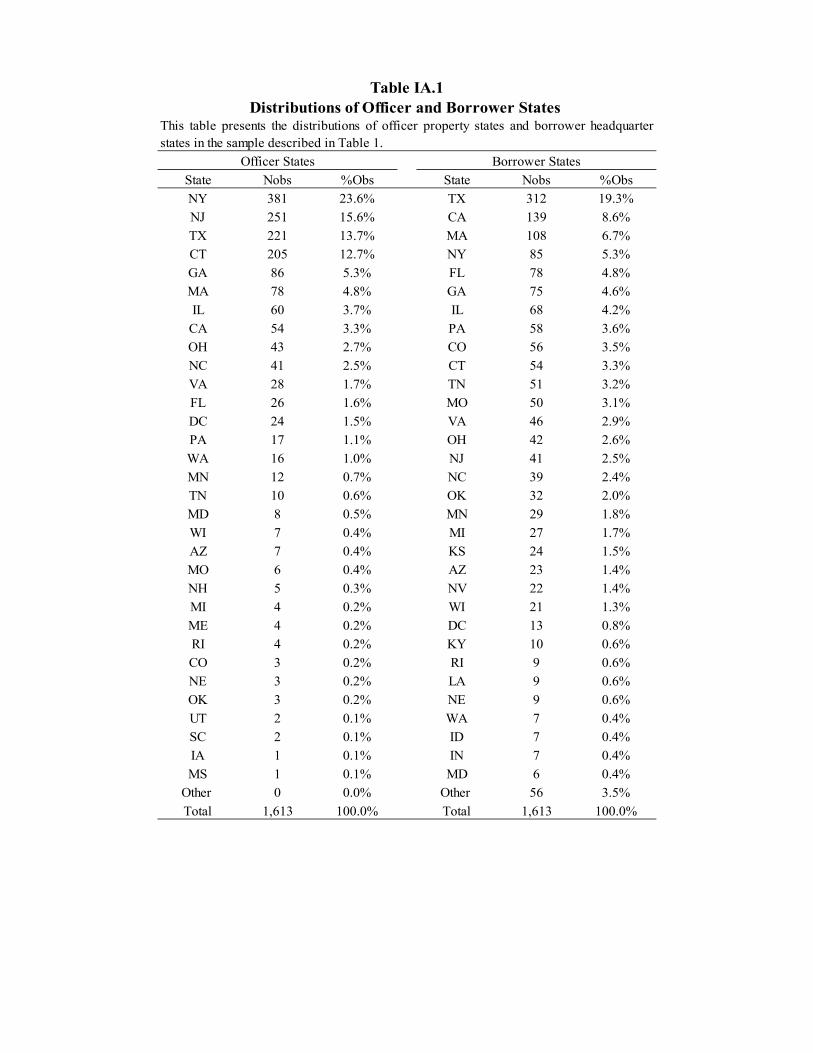
In Table IA.1 and Figure IA.1 we present the distribution of our sample loan officer addresses and borrower headquarters across states. Both loan officer properties and borrower headquarters cover a wide range of states. Yet, there is a significant geographical separation between them. For example, New York, Connecticut, and New Jersey represent 52 percent of officers’ states and only 11 percent of borrower states.

4. Link Between Corporate Loan Spreads and Aggregate Fluctuations in Officer Housing Price Experiences

We examine the link between aggregate fluctuations in officers’ recent housing price growth experiences and corporate loan spreads. We start with graphical evidence. Figure IA.2 illustrates loan officers’ average local housing price growth (past 12 months) together with average loan spreads. The solid line represents average corporate loan spreads across all loans issued to public U.S. firms in Dealscan during our sample period. The dashed line represents the average housing price growth in the 20-mile neighborhood around our sample loan officers, and the dotted line indicates the average state-level House Price Index (HPI) growth across all the states that have at least one loan officer real estate property. Both measures capture average experiences in the past 12 months. There is a clear negative link between local housing price growth and corporate credit spreads over time.

Second, we analyze this same link using a regression analysis. Using loan-level data, we regress log of loan spreads on the average housing price growth experiences across officers in our data over the past year. Note that this explanatory variable only changes in the time series. When computing this average, we use the housing price growth around the properties of all officers in our data. As we aggregate the past growth around these properties, we use housing price data at three different geographic levels where properties are located: 20-mile neighborhoods, county, and state. This leads to three different measures of housing price growth experiences.

Table IA.2 shows the results. In columns (1) through (3), we show the baseline results with the three measures above. In columns (4) through (6), we add controls for macroeconomic conditions such as S&P index stock returns and GDP growth. We also control for the changes in aggregate lending policies, measured by the equity growth rate and the loan losses of the banking sector.

We find a strong, negative association between aggregate fluctuations in officer housing price growth experiences and corporate credit spreads. This result shows that, during the credit cycle we analyze, corporate credits have significantly lower spreads following more positive aggregate experiences by loan officers. To see the economic importance of this link note that Local HPGrowth (Year -1) drops by approximately 20 percentage points between its top and bottom in Figure IA.1. Column (4) implies that this leads to a reduction in the log of loan spreads by 0.32 = 0.2 × 1.6, which represents approximately 213bp × 0.32 = 68 bp (using mean for loan spreads in Table 1).

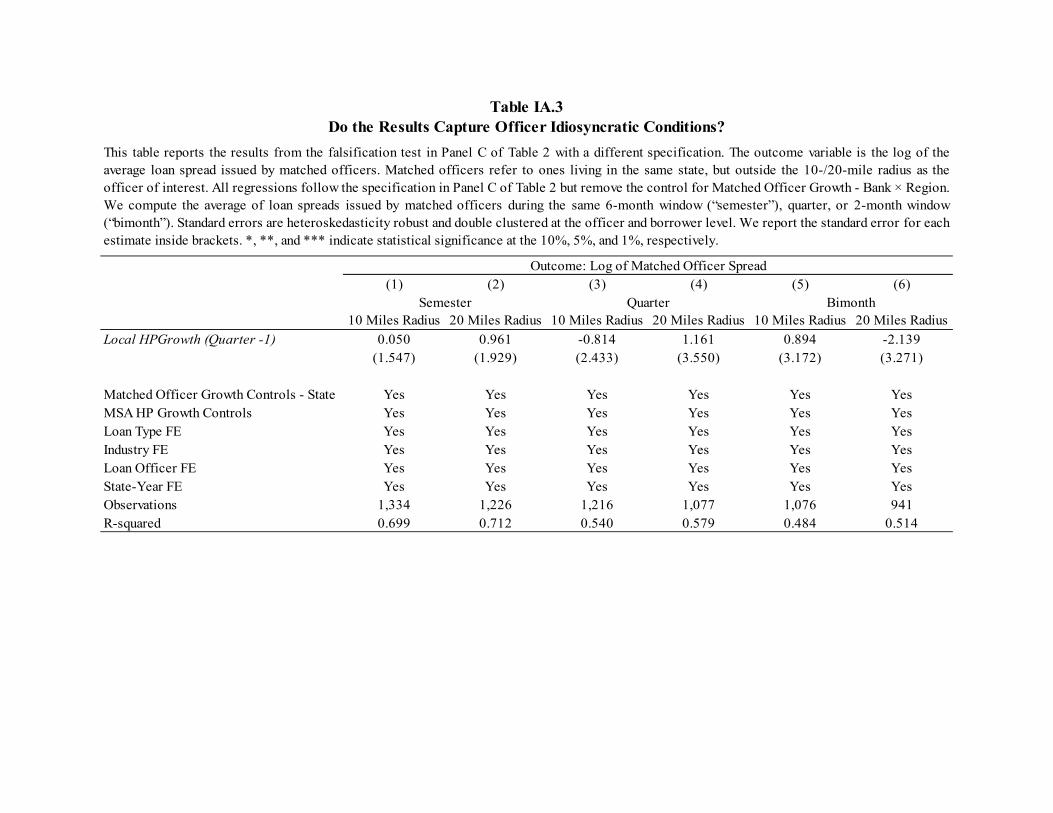
5. Do the Results Capture Officer Idiosyncratic Conditions?

We replicate the falsification test implemented in Panel C of Table 2 using a different specification. In this alternative specification, we exclude the controls Matched Officer Growth - Bank × Region. The exclusion of these controls allows us to have a larger sample and more precise estimates and we use this alternative specification in the paper when estimating interactions of our main effects. Here, we illustrate that this alternative specification also captures officer idiosyncratic conditions as we mention in the text. See Section 3.1 for a discussion of this test.

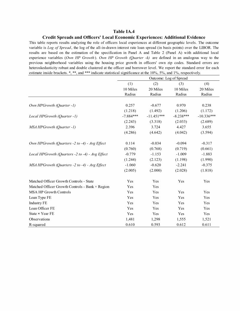
6. Local Experiences at Different Geographic Levels

We expand the baseline specification in Equation (1) by adding officers’ recent housing growth experiences at the zip code level. Table IA.4 presents the results. We continue to find that the effect of local housing growth is concentrated at the neighborhood level.

7. Robustness of Results to Subperiods: Additional Evidence

We provide additional evidence that our results are not driven by specific subperiods. We repeat the baseline analysis by removing every two-year interval in our sample period. These intervals include 1999—2000, 2001—2002, …, 2011—2012. Table IA.5 reports the results. In each subsample, our results remain statistically significant and economically similar to our baseline results. This evidence complements our analysis in the paper showing that our effects are not concentrated during the financial crisis and remain important outside this subperiod. Overall, the results from this set of analyses suggest that our base findings are unlikely to be driven by a specific subperiod of the credit cycle we analyze.

8. Officers’ Economic Experiences and the Pricing of Credit Risk: Additional Evidence

We provide additional evidence on the effect of loan officers’ personal economic experiences on the pricing of credit risk. We extend our results in Table 5 and document that more positive officer experiences are also associated with a weaker link between loan spreads and market benchmarks for these spreads. These market benchmarks measure the average spread for loans originated in the same period as the loan with comparable credit risk (same DD quintile or same credit rating group). Intuitively, such weaker link between the spreads in our sample and market benchmarks captures a reduced sensitivity of lenders to credit risks priced by the loan market. In contrast with the interactions used in Table 5, these benchmarks capture both differences in credit risk across firms and the pricing of such differences by current market conditions. Table IA.6 reports the results. In columns (1) and (2), we show that benchmark spreads are powerful in predicting the loan spread for the borrower of interest. In columns (3) and (4), the results show that this link becomes significantly weaker after more positive officer local experiences or that personal experience effects disproportionally affect riskier loans. These results confirm that more positive lender personal experiences reduce the sensitivity of loans spreads to credit risk or distort the pricing of credit risk.

9. Additional Controls in Cross-Sectional Analyses

We remove the control of Matched Officer Growth - Bank × Region in our cross-sectional analyses because this allows us to have a larger sample and more precise estimates. In the paper, we show that average personal experience effects remain similar with or without these controls. We now examine whether results from the key cross-sectional analyses are robust to the addition of this control. Specifically, we focus on our key cross-sectional tests: the interactions of personal experience effects

with borrowers’ credit risk and real-estate holdings. Table IA.7 reports the results. Column (1) shows the results from the interactive regression of local housing price growth with DDRank. Column (2) shows the results from interactions with DD-Demeaned. Column (3) shows how officer experience effects are related to High RERatio. All of those results are robust to the addition of matched officer growth control by bank and census division. The interaction terms remain statistically significant and imply similar economic magnitudes to the results in Panel A of Tables 5 and 6.

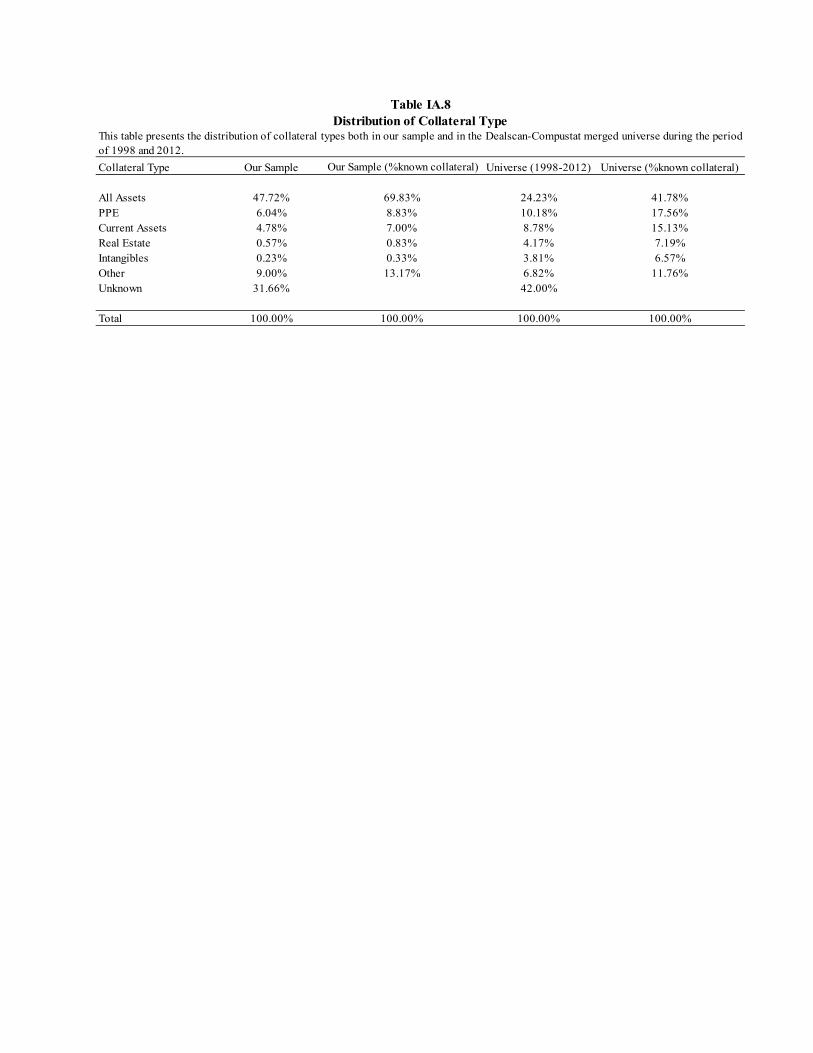
10. Distribution of Collateral Types in Loans

We describe the distribution of collateral type in Dealscan loans in Table IA.8. We report the percentage of loans with the following types of collateral assets: (1) the entirety of borrower assets, (2) property, plant, and equipment (PP&E), (3) current assets, including accounts receivable, inventory, cash and marketable securities, (4) real estate, (5) intangibles and patents, (6) other, including ownership of options and warrants, as well as agency guarantee, and (7) unknown collateral type. We report the distribution both for our sample of loans and for the entire Dealscan universe. We also report the shares of collateral types (1) to (6) as percentage of known collateral types, i.e. excluding cases with unknown collateral.

In our sample, the most common type of collateral is all assets of the borrower, which capture 70 percent of the cases with known collateral. Real estate asset values could influence the collateral value of a loan when the loan is backed by all assets, PP&E, and real estate properties. These cases collectively account for 80 percent of the cases with known collateral in our sample, and 67 percent of loans with known collateral in the Dealscan universe. These patterns are consistent with industry documentation discussed in Section 3.4.

11. Real Estate Holdings and Credit Risk

We examine whether higher credit risk is associated with a larger share of real estate holdings. We regress firms’ real estate ownership on DDRank, which captures firms’ quintile in terms of their distance-to-default (see Section 3.3). Higher values of DDRank capture quintiles with lower credit risk.

Table IA.9 reports the results. We measure real estate ownership using the four measures in Table 6. We also test the relation between credit risk and real estate holdings in our sample and the Dealscan-Compustat universe of loans. Columns (1) to (4) report the results using the Dealscan-Compustat universe and columns (5) through (8) report the results from our sample. Across all measures of real estate ownership and both sample choices, we do not find evidence suggesting that real estate ownership is positively associated with credit risk. If anything, results from columns (1) through (4) suggests that higher credit risk is associated with a lower share of real estate holdings. Moreover, this link is economically weak. For example, in column (1), a reduction in credit risk by one quintile of DD predicts an increase in RERatio equal to 0.8%, which represents 0.8/24 = 3.3 percent of the average value of RERatio (see Table 1 for this average value). These patterns are consistent with the fact that real estate holdings are more important among firms that are larger, older, and more profitable (Chaney, Sraer, and Thesmar (2012)).

12. First-Stage Results from IV Regressions

In Table IA.10, we report the first-stage results from the IV regressions used in Panel B of Table 6 (columns (1) and (2)). These IV regressions analyze the differential effect of economic shocks between years t-5 and t (Shock) on the net debt issuance of real-estate intensive firms, captured by higher values of RERatio (see Table 6). In these first-stage regressions, the dependent variable is Shock × RERatio, which captures this differential shock on real-estate intensive firms. In column (1), Shock is the housing

price growth in the MSA of the firm’s headquarter (HP Growth), and HP Growth × RERatio can be interpreted as a shock to the value of firms’ real estate assets. In column (2), Shock is the county-level employment growth around the firm’s headquarter. RERatio is defined as the ratio of net real estate assets (land and improvements, buildings, and construction in progress) over total net PPE. RERatio is defined as the value of this ratio at t-5 for all years up to 1998. Because of data availability, this ratio is measured at 1993 from 1999 on. The sample includes all non-financial and non-utility firms in Compustat without missing values for RERatio (firms need to be present in 1993 or earlier).

Column (1) in Table IA.10 follows Carvalho (2018) and uses the triple interaction of RERatio with measures of geographically-determined land unavailability at the MSA level (Uland1 to Uland5) and national real estate price growth (NPGrowth) as instruments for RERatio × HP Growth. These measures capture five geographic features of MSAs (based on satellite data) that limit the availability of land for construction, i.e. shares of a 50 km radius around the city’s centroid covered by the ocean, covered by open water, with high slopes, with woody wetlands, and with herbaceous wetlands. The motivation for this approach is the idea that increases in real estate prices can be offset by increased construction activity, which lowers prices through housing supply, but this mechanism is muted when there is land less available. Therefore, land availability can be key for predicting which areas have a greater exposure to national-level shocks to real estate price growth. These characteristics can matter to different degrees and including them separately allows them to have different effects. In sum, this differential exposure of areas to changes over time in national conditions (Uland × NPGrowth) predicts differences in local real estate price growth (HP Growth). As we interact these predicted local shocks with firms’ real estate share, we arrive at the triple interaction described above (see Carvalho (2018) for more details). All variables included as controls are listed in Table IA.10. Firm characteristics (Size, Age, and Cash Flow) are measured in year t -5 and are defined in the same way as in our main results.

Column (2) applies a Bartik instrument that projects national employment growth to the state level. Bartik is given by ∑ 𝑠 𝑁𝐺 , where i denotes each industry in the state, 𝑠 measures the share of the industry in the state (employment) at year t-5, and 𝑁𝐺 measures the national-level growth of the industry (excluding the state) between years t-5 and t. This predicts shocks to state employment growth between years t-5 and t using national-level shocks and differences in the initial industry composition of states, i.e. differences in state exposures to national shocks. As in the case of column (1), all variables included as controls are listed in Table IA.10.

13. Link Between Borrower-Loan Characteristics and Lead Arranger Share

We complement our analysis in Section 3.5 by examining the link between share of loans retained by lead arrangers in a syndicate and the characteristics of borrowers and the lending syndicate. Table IA.11 reports these results. We regress the lead arranger share on the borrower’s Size, Analyst Coverage, DDRank, and whether the loan has a single lead arranger (Single Lead). We use the same sample as in our main results, with the same set of controls and fixed effects. This is intended to capture the link between each characteristic and the lead share in our analysis. When missing, we impute lead arranger shares based on syndication structure, following Chodorow-Reich (2014). Specifically, we use the average lead share in all other Dealscan loans with the same loan structure (number of participants and number of lead banks).

In a first set of results (columns (1) to (3)), we connect borrower characteristics (Size, Analyst Coverage, and DDRank) to this lead arranger share. The goal of these results is to provide additional support for the view that lead arrangers are more important in such loans and need to have more “skin in the game”. A syndicate loan can create a conflict of interest between lead arrangers and other lending participants, as lead banks need to incur costly screening and monitoring activities on behalf of all lenders but retain

only a portion of the loan. Therefore, in the presence of information asymmetry between lead arrangers and other loan participants, leads should hold a larger share of syndicated loans to mitigate this potential conflict of interest. In other words, when lead banks play a more important role in these loans because of their greater ability to evaluate risks and monitor borrowers, other participants should expect them to invest more in the loan. Sufi (2007) discusses this idea and provides evidence supporting it. In our discussion in Section 3.5, we argue that the greater information asymmetry associated with smaller borrowers and borrowers with less analyst coverage should lead to an increased importance of lead arrangers. We also argue that lead arrangers should plausibly perform a more important role in riskier loans. We now confirm that these borrower characteristics are associated with larger lead shares in syndicated loans. In Section 3.5, we also argue that lead banks should be more important in loans with a single lead. Column (4) also shows that having a single lead is a strong predictor of the lead share in these loans. Recall that all these characteristics predicting a higher lead share are associated with stronger officer personal experience effects on loan spreads in our analysis. Therefore, our collective evidence illustrates that the officer effects we analyze are stronger in contexts where their lead banks are predicted to play a more important role.

14. Further Addressing Concern About Borrower Fundamentals

We provide additional evidence addressing a concern that our results could be driven by borrower fundamentals. One possibility is that local conditions in officers’ neighborhoods capture valuable information for predicting their borrowers’ credit risk. Given our identification strategy (see Section 2), this concern will only be relevant if officers’ idiosyncratic conditions within their state predict the fundamentals of non-local borrowers. We note that Panel B of Table 7 documents that our main results are not more important when local officer conditions are more likely to be informative about borrower fundamentals (see Section 3.4). In Table IA.12, we design two subsample tests to further address this possibility. First, we remove cases where the distance between borrowers’ headquarters and their loan officers’ properties is at the bottom quartile of our sample. Second, we exclude cases where borrowers’ industries are highly represented in the local areas surrounding loan officers’ properties (top quartile in our sample). Industry representation is defined as the ratio of the share of local county employment by the borrower’s industry (defined at the 3-digit NAICS level) to this same industry share at the national level. Specifically, the ratio is defined as 𝐸𝑚𝑝 , , /𝐸𝑚𝑝 , 𝐸𝑚𝑝 , , /𝐸𝑚𝑝 , , where j is the borrower’s industry, and c is the loan officer’s county, and t represents time. After calculating this ratio for every quarter, we take the average values across the four quarters prior to loan origination. Panel A of Table IA.12 shows that our results are unchanged when we use these alternative samples.

A related possibility is that recent local conditions predict differences in spreads because they affect lenders’ choice of borrowers. If this selection effect drives our results, we should expect our findings to become significantly weaker after the inclusion of important controls for borrower credit risk. Panel B of Table IA.12 shows that our results remain economically similar as we drop and add important controls for credit risk. In Columns (1) and (2), we control for DD Rank × year fixed effects. In columns (3) and (4), we add the following additional credit risk controls: DDRank, the benchmark credit spread based on DD quintiles, and the benchmark credit spread based on credit rating category. In columns (5) and (6), we remove credit risk controls such as leverage and equity volatility from the baseline regressions. Our results are highly stable to the variation of these controls. This suggests that this selection effect is unlikely to be important in our setting.

15. Additional Robustness Analysis

In Table IA.13, we present results from additional robustness analyses that examine the choice of controls and sample construction. Panel A reports results when we remove controls for other loan

contract terms such as loan maturity and loan size. Column (1) shows the results from the baseline specification (column (2) of Panel A in Table 2). In column (2), we examine the robustness of the interactive effect of local housing price growth and firms’ real estate ownership. Our main results remain similar without these controls for other loan contract terms. Panel B reports results related to sample construction. In column (1), we restrict the sample to officers owning properties in only one state. In column (2), we restrict the sample to loans with one or two lead officers. In column (3), we retain only the largest facility in a loan deal. Our results persist across all alternative sampling choices.

16. Additional Loan Outcomes

We examine the effect of officer local experiences on additional outcomes of the loans in our data. Panels A and B of Table IA.14 analyze our main results with these additional loan outcomes as the dependent variable. We estimate both the average effect of officer personal experience effects (Panel A) and the differential effect on real estate intensity (Panel B). Our preferred specification is the one in Panel B, which focuses on the differential effect of personal experience effects on firms that hold real estate assets and is motivated by the specific mechanism we analyze.

Intuitively, increased lender optimism about the value of borrowers’ assets could also increase the supply of credit by officers’ lead banks. As discussed in Section 1.3, the lead bank holds a share of the loan they originate. Therefore, the idiosyncratic effects on their supply of credit should be reflected in a larger share by the lead bank on the loans they originate (other participants are not directly affected by the personal experience effects we analyze). One challenge in testing this idea is the presence of data limitations. We cannot measure the share of syndicated loans allocated to officers’ lead banks for most loans. This share has to be predicted using the loan structure (number of participants and leads) and this introduces measurement error on this outcome. This same issue also limits our ability to analyze the dollar amount of the loan allocated to the officer’s lead bank. On the other hand, the lead bank plays an important role evaluating risks and setting the spread for the entire loan, and this spread can be directly measured. Therefore, this measurement issue is not present for loan spreads.

We find that more positive local experiences are associated with larger loan shares for the officers’ banks, but this effect is not statistically significant and is economically smaller than the one for loan spreads. For example, the magnitude of the effect in column (1) (Panel B of Table IA.14) can be directly compared to the one in Table 6 (column (6) in Panel A). One potential explanation for this weaker effect on loan shares is the measurement issue described above.

Another possibility is that increased lender optimism leads to less strict loan covenants. In theory, this connection between lender beliefs about the value of borrowers’ assets and covenants is less clear than the connection between these beliefs and loan spreads. Loan spreads should be shaped by these specific beliefs because these asset values determine the recovery of lenders in case of default, and directly shape returns on the loan. This effect is intuitive and also emphasized by practitioners in this market (see Section 3.4). In principle, this increased protection against default could also reduce the need for monitoring and setting strict loan covenants, but this effect is less direct.2 We estimate our main results using loan strictness as the outcome variable, following the measure proposed by Murfin (2012). We find that more positive officer experiences lead to less strict loan covenants but, as in the previous case, this effect is statistically insignificant and economically smaller.

Finally, we also examine effects for the loan maturity and the total loan size. In the context of our preferred specification, these results show no clear effects on loan maturity and the total loan amount

2 Of course, there are other supply-side factors that could have a stronger effect on loan covenants (see Murfin (2012)). We are here considering these specific shifts in beliefs about the value of borrowers’ assets.

(columns (4) and (5), Panel B of Table IA.14). We note that, in theory, the potential connection between lender beliefs about borrowers’ asset values and loan maturity is also less clear than the connection of these beliefs with loan spreads. This can rationalize the contrast between our findings for loan spreads and loan maturity. When interpreting the total loan amount result, recall that our empirical analysis focuses idiosyncratic shocks to officers’ lead banks. As other loan participants are not directly affected by this shock, the effect on officers’ bank has to be sufficiently strong to be detected in the data. In contrast, as discussed above, the lead bank plays an important role evaluating risks and setting the spread for the entire loan.

As we consider the broader implications of our results, we note the following important points. First, our findings do not suggest that lenders’ beliefs about borrower asset values do not significantly matter for loan amounts. We focus on idiosyncratic shocks to certain lead banks for identification reasons. More broadly, aggregate conditions affecting the beliefs of all participants in a syndicate could have stronger effects on loan amounts.

Additionally, we note that distortions in the pricing of credit risk and excessive fluctuations in credit spreads play a central role in narratives and models of distorted lender beliefs and credit cycles (e.g., Bordalo, Gennaioli, Shleifer (2018)), and that previous research on credit cycles has relied on credit spreads to capture shifts in lender optimism across the credit cycle (e.g., López-Salido, Stein, and Zakrajšek (2017), Sufi, Mian, and Verner (2017)). Our findings on loan spreads are directly connected to these important ideas and empirical patterns.

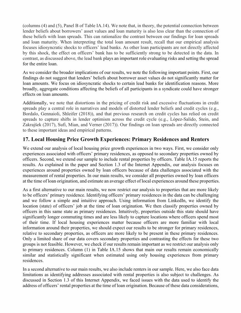
17. Local Housing Price Growth Experiences: Primary Residences and Renters

We extend our analysis of local housing price growth experiences in two ways. First, we consider only experiences associated with officers’ primary residences, as opposed to secondary properties owned by officers. Second, we extend our sample to include rental properties by officers. Table IA.15 reports the results. As explained in the paper and Section 1.3 of the Internet Appendix, our analysis focuses on experiences around properties owned by loan officers because of data challenges associated with the measurement of rental properties. In our main results, we consider all properties owned by loan officers at the time of loan origination, and estimate an average effect of local experiences around these properties.

As a first alternative to our main results, we now restrict our analysis to properties that are more likely to be officers’ primary residence. Identifying officers’ primary residences in the data can be challenging and we follow a simple and intuitive approach. Using information from LinkedIn, we identify the location (state) of officers’ job at the time of loan origination. We then classify properties owned by officers in this same state as primary residences. Intuitively, properties outside this state should have significantly longer commuting times and are less likely to capture locations where officers spend most of their time. If local housing experiences matter because officers are more familiar with local information around their properties, we should expect our results to be stronger for primary residences, relative to secondary properties, as officers are more likely to be present in these primary residences. Only a limited share of our data covers secondary properties and contrasting the effects for these two groups is not feasible. However, we check if our results remain important as we restrict our analysis only to primary residences. Column (1) in Table IA.15 shows that main our results remain economically similar and statistically significant when estimated using only housing experiences from primary residences.

In a second alternative to our main results, we also include renters in our sample. Here, we also face data limitations as identifying addresses associated with rental properties is also subject to challenges. As discussed in Section 1.3 of this Internet Appendix, we faced issues with the data used to identify the address of officers’ rental properties at the time of loan origination. Because of these data considerations,

we focused on properties owned by officers in our main results, and include this extension to renters as a robustness check. We measure housing price growth experiences in the same way as in the case of property owners using the location of rental properties at the time of loan origination. We combine our data on local experiences by owners and renters and start by estimating an average effect across these two groups. Column (2) of Table IA.15 shows that our results remain economically similar and statistically significant as we combine these two groups of experiences together. We then estimate separate effects for owners and renters (column (3) of Table IA.15) in this combined sample. We also estimate our effects using only the sample renters (column (4) of Table IA.15). If local housing price growth experiences matter because officers are more familiar with local information around their properties, our results should remain relevant among renters. Alternatively, as discussed in the paper (e.g., Section 2.2), our results could capture the effect of officers’ personal wealth experiences. In other words, officers’ might overweight changes in housing prices that affect their personal wealth when forming beliefs about national real estate prices. If this is the case, our effects should not be present among renters and should be only important for property owners. We note that our effects are only statistically significant for property owners but that they have the same sign with a smaller magnitude for renters. The magnitude of the results using only renters (column (4)) is smaller but comparable to the one for primary residences (column (1)) and owners and renters combined (column (2)). As the data for renters is less accurate, this pattern could reflect greater measurement error and the smaller sample size associated with our sample of renters. In sum, our results remain similar as we include both owners and renters but our data does not allow us to differentiate in a clear way between the effects for owners and renters.

References

Bordalo, Pedro, Nicola Gennaioli, and Andrei Shleifer, 2018, Diagnostic expectations and credit cycles, Journal of Finance 73, 199-227.

Carvalho, Daniel, 2018, How do financing constraints affect firms’ equity volatility?, Journal of Finance 73, 1139-1182.

Chaney, Thomas, David Sraer, and David Thesmar, 2012, The collateral channel: How real estate shocks affect corporate investment, American Economic Review 102, 2381-2409.

Cheng, Ing-Haw, Sahil Raina, and Wei Xiong, 2014, Wall Street and the housing bubble, American Economic Review 104, 2797-2829.

Chodorow-Reich, Gabriel, 2014, The employment effects of credit market disruptions: Firm-level evidence from the 2008-9 financial crisis, Quarterly Journal of Economics 129, 1-59.

López-Salido, David, Jeremy Stein, and Egon Zakrajšek, 2017, Credit-market sentiment and the business cycle, Quarterly Journal of Economics 132, 1373-1426.

Mian, Atif, Amir Sufi, and Emil Verner, 2017, Household debt and business cycles worldwide, Quarterly Journal of Economics 132, 1755-1817.

Murfin, Justin, 2012, The supply-side determinants of loan contract strictness, Journal of Finance 67, 1565-1601.

Pool, Veronika K., Noah Stoffman, and Scott E. Yonker, 2012, No place like home: Familiarity in mutual fund manager portfolio choice, Review of Financial Studies 25, 2563-2599.

Sufi, Amir, 2007, Information asymmetry and financing arrangements: Evidence from syndicated loans, Journal of Finance 62, 629-668.

Figure IA.1Officer Property and Borrower Headquarter Location

This figure shows the all counties with officer properties or borrower headquarters in our sample described in Table1. Panel A shows all counties where there is at least one loan officer property in this sample. Panel B shows allcounties where there is at least one borrower headquarter in this sample.

Panel A: Distribution of Officer Property Counties

Panel B: Distribution of Borrower Headquarter Counties

Figure IA.2Credit Spreads and Lenders' Recent Economic Experiences: Aggregate Patterns

This figure shows aggregate patterns for corporate credit spreads on bank loans and measures of the recenteconomic experiences of corporate loan officers between 2004 and 2012. Loan Spreads measures the average valuefor the all-in-drawn interest rate spreads in basis points over the LIBOR in a large sample of corporate loans. Thissample covers all loans in Dealscan that can be matched to Compustat. Avg State HP Growth and Avg Local HPGrowth measure the weighted average of recent housing price growth in the states and neighborhoods where theproperties of corporate loan officers in our data are located, respectively. These averages are computed using theshare of properties in our data located in a state or zip code as weights. These shares are constant over time andbased on our entire dataset. Information on state-level housing prices comes from the Office of Federal HousingEnterprise Oversight (OFHEO). Neighborhood growth is the average growth of housing prices (Zillow) across thezip codes in 20-mile neighborhoods centered around officers' properties. Both measures of recent housing pricegrowth is calculated as the cumulative growth rates between quarters t -1 and t -5 (annual past growth).

-10%

-5%

0%

5%

10%

15%

200

220

240

260

280

300

320

340

360

380

400

Loan Spreads Avg Local HP Growth (Zillow)

Avg State HPI Growth (OFHEO)

State Nobs %Obs State Nobs %Obs

NY 381 23.6% TX 312 19.3%

NJ 251 15.6% CA 139 8.6%

TX 221 13.7% MA 108 6.7%

CT 205 12.7% NY 85 5.3%

GA 86 5.3% FL 78 4.8%

MA 78 4.8% GA 75 4.6%

IL 60 3.7% IL 68 4.2%

CA 54 3.3% PA 58 3.6%

OH 43 2.7% CO 56 3.5%

NC 41 2.5% CT 54 3.3%

VA 28 1.7% TN 51 3.2%

FL 26 1.6% MO 50 3.1%

DC 24 1.5% VA 46 2.9%

PA 17 1.1% OH 42 2.6%

WA 16 1.0% NJ 41 2.5%

MN 12 0.7% NC 39 2.4%

TN 10 0.6% OK 32 2.0%

MD 8 0.5% MN 29 1.8%

WI 7 0.4% MI 27 1.7%

AZ 7 0.4% KS 24 1.5%

MO 6 0.4% AZ 23 1.4%

NH 5 0.3% NV 22 1.4%

MI 4 0.2% WI 21 1.3%

ME 4 0.2% DC 13 0.8%

RI 4 0.2% KY 10 0.6%

CO 3 0.2% RI 9 0.6%

NE 3 0.2% LA 9 0.6%

OK 3 0.2% NE 9 0.6%

UT 2 0.1% WA 7 0.4%

SC 2 0.1% ID 7 0.4%

IA 1 0.1% IN 7 0.4%

MS 1 0.1% MD 6 0.4%

Other 0 0.0% Other 56 3.5%

Total 1,613 100.0% Total 1,613 100.0%

Table IA.1Distributions of Officer and Borrower States

This table presents the distributions of officer property states and borrower headquarterstates in the sample described in Table 1.

Officer States Borrower States

(1) (2) (3) (4) (5) (6)

Local HPGrowth (Year -1) -3.454*** -1.623***

(0.251) (0.369)

County HPGrowth (Year -1) -3.563*** -1.736***

(0.249) (0.366)

State HPGrowth (Year -1) -5.319*** -3.383***

(0.272) (0.439)

S&P Returns -0.313*** -0.311*** -0.370***

(0.048) (0.048) (0.049)

GDP Growth -0.017** -0.015** -0.004

(0.007) (0.007) (0.007)

Banking Sector Equity Growth -2.121*** -2.025*** -1.203*

(0.701) (0.693) (0.673)

Banking Sector Loan Losses 16.405*** 16.161*** 12.740***

(1.068) (1.071) (1.208)

Firm FE Yes Yes Yes Yes Yes Yes

Loan Type FE Yes Yes Yes Yes Yes Yes

Observations 11,514 11,514 11,514 11,514 11,514 11,514

R-squared 0.379 0.381 0.396 0.408 0.408 0.412

Outcome: Log of Spread

Table IA.2Officers' Personal Economic Experiences and Loan Spreads, Time-Series Evidence

This table reports results connecting changes in corporate loan spreads over time to recent economic conditions in loanofficers' neighborhoods, captured by the average local housing price growth in these areas. The unit of observation is aloan and the sample includes all Dealscan loans matched to U.S. public firms between 2004 and 2012. The dependentvariable is Log of Spread , the log of the all-in-drawn interest rate loan spread (in basis points) over the LIBOR. In eachspecification, the recent local housing growth experience of loan officers is captured by one of the following threevariables. Local HPGrowth (Year -1 ) is the average local housing price growth in the year prior to loan origination. Thisaverage is computed using all neighborhoods (20-miles radius) around officer properties in our data (fixed set ofproperties over time covering our entire sample). County HPGrowth (Year -1 ) is the average housing price growth in thecounties of loan officers' properties in the year prior to loan origination. State HPGrowth (Year -1 ) is the averagehousing price growth in the state of loan officers' properties (OFHEO data) in the year prior to loan origination. Thisaverage across counties (states) is measured every quarter using all counties (states) with officer properties in our data.Each county (state) is weighted using the share of total officer properties in our data (constant weights over time).Neighborhood (county) growth is the average growth of housing prices (Zillow) across the zip codes in the neighborhood(county) where officers' properties are located. All results include the following controls: Loan Size , Loan Maturity , Equity Volatility , Size , Firm Age , Profitability , Tangibility , M/B , Leverage , and Rated . These borrowercharacteristics are measured in the year prior to the loan. The results in columns (4) to (6) also include the followingadditional controls: S&P Returns , GDP Growth , Banking Sector Equity Growth , and Banking Sector Loan Losses . S&P Returns is the average S&P 500 returns during the four quarters prior to loan origination; GDP Growth is theaverage growth rate of U.S. GDP in the past four quarters; Banking Sector Equity Growth is the average growth rate ofequity to asset ratio of the U.S. banking sector in the past four quarters; and Banking Sector Loan Losses measures theaverage loan losses (scaled by total equity capital) of the U.S. banking sector in the past four quarters. Standard errors areheteroskedasticity robust and clustered by borrower. We report the standard error for each estimate inside brackets. *, **,and *** indicate statistical significance at the 10%, 5%, and 1%, respectively.

(1) (2) (3) (4) (5) (6)

10 Miles Radius 20 Miles Radius 10 Miles Radius 20 Miles Radius 10 Miles Radius 20 Miles Radius

Local HPGrowth (Quarter -1) 0.050 0.961 -0.814 1.161 0.894 -2.139(1.547) (1.929) (2.433) (3.550) (3.172) (3.271)

Matched Officer Growth Controls - State Yes Yes Yes Yes Yes YesMSA HP Growth Controls Yes Yes Yes Yes Yes YesLoan Type FE Yes Yes Yes Yes Yes YesIndustry FE Yes Yes Yes Yes Yes YesLoan Officer FE Yes Yes Yes Yes Yes YesState-Year FE Yes Yes Yes Yes Yes YesObservations 1,334 1,226 1,216 1,077 1,076 941R-squared 0.699 0.712 0.540 0.579 0.484 0.514

Semester Quarter Bimonth

Outcome: Log of Matched Officer Spread

Table IA.3Do the Results Capture Officer Idiosyncratic Conditions?

This table reports the results from the falsification test in Panel C of Table 2 with a different specification. The outcome variable is the log of theaverage loan spread issued by matched officers. Matched officers refer to ones living in the same state, but outside the 10-/20-mile radius as theofficer of interest. All regressions follow the specification in Panel C of Table 2 but remove the control for Matched Officer Growth - Bank × Region. We compute the average of loan spreads issued by matched officers during the same 6-month window (“semester”), quarter, or 2-month window(“bimonth”). Standard errors are heteroskedasticity robust and double clustered at the officer and borrower level. We report the standard error for eachestimate inside brackets. *, **, and *** indicate statistical significance at the 10%, 5%, and 1%, respectively.

(1) (2) (3) (4)

10 Miles Radius

20 Miles Radius

10 Miles Radius

20 Miles Radius

Own HPGrowth (Quarter -1) 0.257 -0.677 0.970 0.238

(1.218) (1.492) (1.206) (1.172)

Local HPGrowth (Quarter -1) -7.884*** -11.451*** -8.238*** -10.336***

(2.243) (3.318) (2.033) (2.689)

MSA HPGrowth (Quarter -1) 2.396 3.724 4.427 3.655

(4.286) (4.642) (4.042) (3.594)

Own HPGrowth (Quarters -2 to -4) - Avg Effect 0.114 -0.034 -0.094 -0.317

(0.760) (0.768) (0.719) (0.661)

Local HPGrowth (Quarters -2 to -4) - Avg Effect -0.779 -1.153 -1.009 -1.883

(1.244) (2.123) (1.198) (1.990)

MSA HPGrowth (Quarters -2 to -4) - Avg Effect -1.060 -0.620 -2.241 -0.375

(2.005) (2.000) (2.028) (1.818)

Matched Officer Growth Controls - State Yes Yes Yes Yes

Matched Officer Growth Controls - Bank × Region Yes Yes

MSA HP Growth Controls Yes Yes Yes Yes

Loan Type FE Yes Yes Yes Yes

Industry FE Yes Yes Yes Yes

Loan Officer FE Yes Yes Yes YesState × Year FE Yes Yes Yes Yes

Observations 1,481 1,298 1,555 1,521

R-squared 0.610 0.593 0.612 0.611

Table IA.4Credit Spreads and Officers' Local Economic Experiences: Additional Evidence

This table reports results analyzing the role of officers local experiences at different geographic levels. The outcomevariable is Log of Spread , the log of the all-in-drawn interest rate loan spread (in basis points) over the LIBOR. Theresults are based on the estimation of the specification in Panel A and Table 2 (Panel A) with additional localexperience variables (Own HP Growth ). Own HP Growth (Quarter -k) are defined in an analogous way to theprevious neighborhood variables using the housing price growth in officers' own zip codes. Standard errors areheteroskedasticity robust and double clustered at the officer and borrower level. We report the standard error for eachestimate inside brackets. *, **, and *** indicate statistical significance at the 10%, 5%, and 1%, respectively.


(1) (2) (3) (4) (5) (6) (7)Years Excluded: 1999-2000 2001-2002 2003-2004 2005-2006 2007-2008 2009-2010 2011-2012

Local HPGrowth (Quarter -1) -12.028*** -11.833*** -9.932*** -10.510*** -13.271*** -10.893*** -14.563**(3.325) (3.260) (3.521) (3.700) (3.463) (4.038) (5.620)

Local HPGrowth (Quarters -2 to -4) - Avg Effect -1.183 -0.508 -0.305 -2.889 -3.646* -1.688 0.765(1.836) (1.841) (1.917) (2.164) (1.890) (2.536) (2.524)

Matched Officer Growth Controls - State Yes Yes Yes Yes Yes Yes YesMatched Officer Growth Controls - Bank × Region Yes Yes Yes Yes Yes Yes YesMSA HP Growth Controls Yes Yes Yes Yes Yes Yes YesLoan Type FE Yes Yes Yes Yes Yes Yes YesIndustry FE Yes Yes Yes Yes Yes Yes YesLoan Officer FE Yes Yes Yes Yes Yes Yes YesState-Year FE Yes Yes Yes Yes Yes Yes YesObservations 1,302 1,259 1,206 1,113 1,060 1,051 906R-squared 0.590 0.583 0.600 0.611 0.652 0.585 0.632


Table IA.5Results Across Subperiods: Additional Evidence

This table shows the robustness of our results to removing every two-year interval from the sample. The regressions follow the baseline specification,shown in column (2) of Panel A in Table 2. Standard errors are heteroskedasticity robust and double clustered at the officer and borrower level. Wereport the standard error for each estimate inside brackets. *, **, and *** indicate statistical significance at the 10%, 5%, and 1%, respectively.

(1) (2) (3) (4)

Benchmark Defined by: Distance-to-Default Credit Rating Distance-to-Default Credit Rating

Benchmark Spread (Mkt Adjusted) 0.295*** 0.420** 0.213*** 0.307**

(0.063) (0.164) (0.075) (0.152)

Local HPGrowth (Quarter -1) -6.939*** -7.295***

(2.584) (2.611)

LHPGrowth (Quarter -1) × Benchmark Spread (Mkt Adjusted) -19.344*** -13.554**

(6.595) (5.655)

Scaled Effect -13.720*** -10.360**

(4.678) (4.322)

Matched Officer Growth Controls - State Yes Yes

MSA HP Growth Controls Yes Yes



Loan Officer FE Yes Yes Yes Yes

State-Year FE Yes Yes Yes Yes

Observations 1,449 1,574 1,419 1,539

R-squared 0.564 0.567 0.581 0.611

Outcome: Log of Spread, Market Adjusted

Table IA.6Officers' Economic Experiences and the Pricing of Credit Risk, Additional Evidence

This table examines the interactive effect of officer local housing price growth and borrower credit risk on market adjusted log of spread. Borrower creditrisk is measured by Benchmark Spread , the average spread (also market adjusted) among a group of borrowers with similar credit risk profile as theborrower of interest. The benchmark spread is calculated as the average loan spreads issued to firms in the same quintile of distance-to-default during thesame quarter in columns (1) and (3); and as the average loan spreads issued to firms with the same credit rating during the same year in columns (2) and (4).Both benchmarks are defined in quarter/year prior to loan origination. In columns (1) and (2), we report results from linear regressions predicting the loanspread (market adjusted) using the benchmark spreads (also market adjusted). In columns (3) and (4), we report results from the estimation of Equation (2).Scaled effects are calculated as the product of the interactive coefficient and the average gap between the top 50% and bottom 50% values of the benchmarkspreads. All regressions include the set of controls and fixed effects used in Table 3 (columns (1) and (2) of Panel A). We also control for the interactionterms of the variable of interest and the recent histories of local housing price growth as well as those of MSA housing price growth. Standard errors areheteroskedasticity robust and double clustered at the officer and borrower level. We report the standard error for each estimate inside brackets. *, **, and*** indicate statistical significance at the 10%, 5%, and 1%, respectively.

(1) (2) (3)

Local HPGrowth (Quarter -1) -23.381*** -10.933*** -4.672

(5.454) (3.277) (4.875)

LHPGrowth (Quarter -1) × DDRank 5.836***

(1.879)

DDRank -0.099***

(0.025)

LHPGrowth (Quarter -1) × DD-Demeaned 3.346**

(1.336)

DD-Demeaned -0.062***

(0.017)

LHPGrowth (Quarter -1) × High RERatio -14.057**

(6.859)

Scaled Effect 13.777*** 10.619**

(4.435) (4.241)

Matched Officer Growth Controls - State Yes Yes Yes

Matched Officer Growth Controls - Bank × Region Yes Yes Yes

MSA HP Growth Controls Yes Yes Yes

Loan Type FE Yes Yes Yes

Industry FE Yes Yes Yes

Loan Officer FE Yes Yes Yes

State-Year FE Yes Yes Yes

Observations 1,209 1,209 974

R-squared 0.634 0.632 0.665


Table IA.7Cross-Sectional Results with Additional Controls

This table shows the robustness of the cross-sectional results to adding the control for Matched Officer Growth -Bank × Region. Columns (1) and (2) correspond to column (1) and (2) of Table 5 in the paper and column (3)correspond to column (6) of Panel A in Table 6 in the paper. DDRank is the quintile ranking of a firm’s distance-to-default among Dealscan-Compustat universe loans originated in the same quarter. DD-Demeaned is theaverage level of distance-to-default of borrowers within the same quintile category subtracting the average ofdistance-to-default across all Dealscan-Compustat loans issued during the same quarter. High RERatio is anindicator for whether the borrower’s RERatio ranks above the sample median level. Scaled effect equals theinteractive coefficient multiplied by the gap between the conditioning variable's mean in the top 50% and bottom50% of its distribution in our sample. Standard errors are heteroskedasticity robust and double clustered at theofficer and borrower level. We report the standard error for each estimate inside brackets. *, **, and *** indicatestatistical significance at the 10%, 5%, and 1%, respectively.

Collateral Type Our Sample Our Sample (%known collateral) Universe (1998-2012) Universe (%known collateral)

All Assets 47.72% 69.83% 24.23% 41.78%PPE 6.04% 8.83% 10.18% 17.56%Current Assets 4.78% 7.00% 8.78% 15.13%Real Estate 0.57% 0.83% 4.17% 7.19%Intangibles 0.23% 0.33% 3.81% 6.57%Other 9.00% 13.17% 6.82% 11.76%Unknown 31.66% 42.00%

Total 100.00% 100.00% 100.00% 100.00%

Table IA.8Distribution of Collateral Type

This table presents the distribution of collateral types both in our sample and in the Dealscan-Compustat merged universe during the periodof 1998 and 2012.

(1) (2) (3) (4) (5) (6) (7) (8)

Outcome: RERatio REOwner(5%) REOwner(10%) High RERatio RERatio REOwner(5%) REOwner(10%) High RERatio

DDRank 0.008*** 0.031*** 0.031*** 0.030*** 0.010 0.006 -0.003 -0.019

(0.002) (0.004) (0.004) (0.004) (0.008) (0.024) (0.023) (0.019)

Ind FE Yes Yes Yes Yes Yes Yes Yes Yes

Year FE Yes Yes Yes Yes Yes Yes Yes Yes

Observations 44,606 44,606 44,606 44,606 1,021 1,021 1,021 1,021

R-squared 0.196 0.160 0.173 0.157 0.349 0.346 0.349 0.351

Table IA.9Firm Credit Risk and Real-Estate Ownership

This table presents results relating borrowers’ real estate holding and credit risk. The results are based on a linear regression predicting measures of real estateownership with DDRank , the quintile ranking of a firm’s distance-to-default among Dealscan-Compustat universe loans originated in the same quarter. Highervalues of DDRank capture quintiles with lower credit risk. Columns (1) to (4) reports the results using universe Dealscan loans between 1998 and 2012 thatcan be merged with Compustat firms (excluding financial and utility firms). Columns (5) to (8) reports the results using our sample described in Table 1.RERatio stands for the ratio of borrowers’ real estate assets over PP&E. REOwner(5%) is an indicator for whether borrowers’ real estate assets account formore than 5% of PP&E. REOwners(10%) is defined analogously. High RERatio is an indicator for whether the borrower’s RERatio ranks above the samplemedian level. All regressions in this table control for industry and year fixed effects. Standard errors are heteroskedasticity robust and double clustered at theborrower and year level. We report the standard error for each estimate inside brackets. *, **, and *** indicate statistical significance at the 10%, 5%, and 1%,respectively.

Outcome: RERatio × HP Growth Outcome: RERatio × StateEMPGrowth

(1) (2)

Uland_1 -0.060***

(0.016)

Uland_2 -0.030

(0.020)

Uland_3 -0.082

(0.085)

Uland_4 0.026

(0.036)

Uland_5 0.043

(0.039)

NPGrowth × Uland_1 -0.776***

(0.184)


(0.168)

NPGrowth × Uland_3 2.003**

(0.856)


(0.658)

NPGrowth × Uland_5 -0.496

(0.440)

NPGrowth × RERatio 0.595***

(0.113)

Table IA.10First Stage for IV Regression Results

This table presents the first stages for the IV regression results in columns (1) and (2) of Panel B, Table 6. These IVregressions analyze the differential effect of economic shocks between years t -5 and t (Shock ) on the net debt issuance ofreal-estate intensive firms, captured by higher values of RERatio (see Table 6). In these first-stage regressions, thedependent variable is Shock × RERatio , which captures this differential shock on real-estate intensive firms. In column (1),Shock is the housing price growth in the MSA of the firm's headquarter (HP Growth ), and HP Growth × RERatio can beinterpreted as a shock to the value of firms' real estate assets. In column (2), Shock is the county-level employment growtharound the firm's headquarter. RERatio is defined as the ratio of net real estate assets (land and improvements, buildings,and construction in progress) over total net PPE. RERatio is defined as the value of this ratio at t -5 for all years up to1998. Because of data availability, this ratio is measured at 1993 from 1999 on. The sample includes all non-financial andnon-utility firms in Compustat without missing values for RERatio (firms need to be present in 1993 or earlier). Column (1)follows Carvalho (2018, cited in the paper) and uses the triple interaction of RERatio with measures of geographically-determined land unavailability at the MSA level (Uland1 to Uland5 ) and national real estate price growth (NPGrowth ) asinstruments for RERatio × HP Growth . Column (2) applies the Bartik instrument that projects national employment growthto the state level. All regressions in this panel control for industry and year fixed effects. Interactions of MSA real estateprice growth with indicators for firms’ industry are included as controls in column (1). Interactions of state employmentgrowth with indicators for firms’ industry are included as controls in column (2). All other variables listed below are alsoincluded as controls in each case. Firm characteristics (Size , Age , and Cash Flow ) are measured in year t -5. See the textfor variable definitions and discussion of these approaches. Standard errors are heteroskedasticity robust and doubleclustered at the state and year level. We report the standard error for each estimate inside brackets. *, **, and *** indicatestatistical significance at the 10%, 5%, and 1%, respectively.

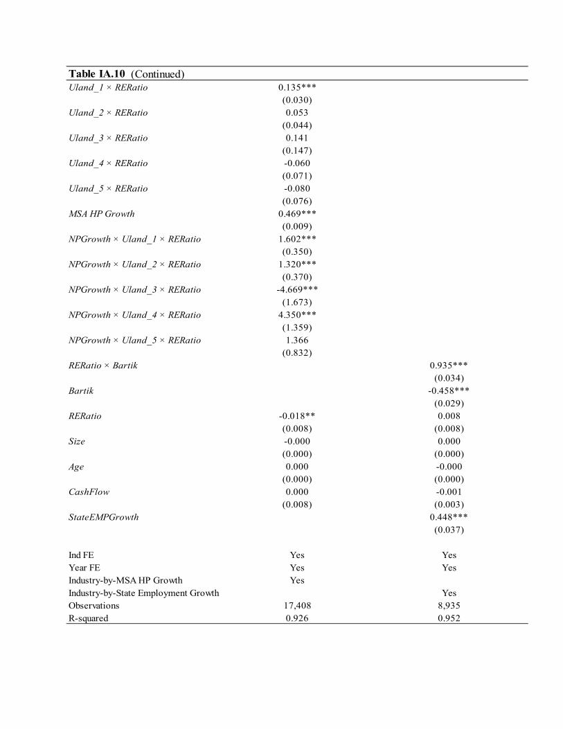
Table IA.10 (Continued)Uland_1 × RERatio 0.135***

(0.030)Uland_2 × RERatio 0.053

(0.044)Uland_3 × RERatio 0.141

(0.147)Uland_4 × RERatio -0.060

(0.071)Uland_5 × RERatio -0.080

(0.076)MSA HP Growth 0.469***

(0.009)NPGrowth × Uland_1 × RERatio 1.602***


(0.370)NPGrowth × Uland_3 × RERatio -4.669***


(1.359)NPGrowth × Uland_5 × RERatio 1.366

(0.832)RERatio × Bartik 0.935***

(0.034)Bartik -0.458***

(0.029)RERatio -0.018** 0.008

(0.008) (0.008)Size -0.000 0.000

(0.000) (0.000)Age 0.000 -0.000

(0.000) (0.000)CashFlow 0.000 -0.001

(0.008) (0.003)StateEMPGrowth 0.448***

(0.037)

Ind FE Yes YesYear FE Yes YesIndustry-by-MSA HP Growth YesIndustry-by-State Employment Growth YesObservations 17,408 8,935R-squared 0.926 0.952

(1) (2) (3) (4)

Size -2.052***

(0.582)

Analyst Coverage -0.220***

(0.079)

DD Rank -0.860*

(0.487)

Single Lead 6.453***

(1.997)

Scaled Effect -5.132*** -2.630*** -2.031*

(1.455) (0.942) (1.148)

Loan and Demographic Controls Yes Yes Yes Yes



Loan Officer FE Yes Yes Yes YesState × Year FE Yes Yes Yes Yes

Observations 1,574 1,458 1,449 1,574

R-squared 0.359 0.356 0.364 0.366

Outcome: Bank Loan Share

Table IA.11Lead Arranger Share and Borrower-Loan Characteristics

This table presents results relating shares retained by lead arranger to borrower and loan characteristics.%LoanShare is the share of the officer's bank (lead arranger) in the loan (in percentage points). When thisvariable is missing, we impute it based on the loan syndication structure (see the text). Size is the log of totalassets. Analyst Coverage is the number of analysts covering the borrower. DDRank is the quintile ranking of afirm’s distance-to-default among Dealscan-Compustat universe loans originated in the same quarter. Single Leadis an indicator for whether the bank is the only lead arranger bank that the borrower has had. All borrowercharacteristics are measured in the year prior to the loan. We control for loan characteristics (Loan Size and Loan Maturity ) and local demographics (Population , Average Home Value , Income per Household , Black Share , and Hispanic Share ). Scaled effect equals the product of the coefficient and variable's mean in the top 50% andbottom 50% of its distribution in our sample. All regressions in this panel control for loan type, industry, loanofficer and state-year fixed effects. Standard errors are heteroskedasticity robust and double clustered at the officer and borrower level. We report the standard error for each estimate inside brackets. *, **, and *** indicatestatistical significance at the 10%, 5%, and 1%, respectively.

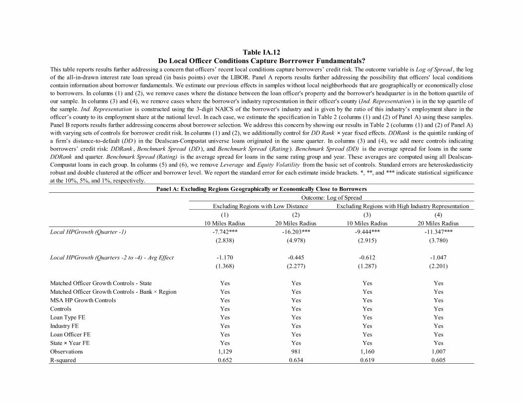
(1) (2) (3) (4)

10 Miles Radius 20 Miles Radius 10 Miles Radius 20 Miles Radius

Local HPGrowth (Quarter -1) -7.742*** -16.203*** -9.444*** -11.347***

(2.838) (4.978) (2.915) (3.780)

Local HPGrowth (Quarters -2 to -4) - Avg Effect -1.170 -0.445 -0.612 -1.047

(1.368) (2.277) (1.287) (2.201)


Matched Officer Growth Controls - Bank × Region Yes Yes Yes Yes


Controls Yes Yes Yes Yes




State × Year FE Yes Yes Yes Yes

Observations 1,129 981 1,160 1,007

R-squared 0.652 0.634 0.619 0.605

Do Local Officer Conditions Capture Borrrower Fundamentals?Table IA.12

Excluding Regions with High Industry Representation

This table reports results further addressing a concern that officers’ recent local conditions capture borrowers’ credit risk. The outcome variable is Log of Spread , the logof the all-in-drawn interest rate loan spread (in basis points) over the LIBOR. Panel A reports results further addressing the possibility that officers' local conditionscontain information about borrower fundamentals. We estimate our previous effects in samples without local neighborhoods that are geographically or economically closeto borrowers. In columns (1) and (2), we remove cases where the distance between the loan officer's property and the borrower's headquarter is in the bottom quartile ofour sample. In columns (3) and (4), we remove cases where the borrower's industry representation in their officer's county (Ind. Representation ) is in the top quartile ofthe sample. Ind. Representation is constructed using the 3-digit NAICS of the borrower's industry and is given by the ratio of this industry’s employment share in theofficer’s county to its employment share at the national level. In each case, we estimate the specification in Table 2 (columns (1) and (2) of Panel A) using these samples.Panel B reports results further addressing concerns about borrower selection. We address this concern by showing our results in Table 2 (columns (1) and (2) of Panel A)with varying sets of controls for borrower credit risk. In columns (1) and (2), we additionally control for DD Rank × year fixed effects. DDRank is the quintile ranking ofa firm’s distance-to-default (DD ) in the Dealscan-Compustat universe loans originated in the same quarter. In columns (3) and (4), we add more controls indicatingborrowers’ credit risk: DDRank , Benchmark Spread (DD ), and Benchmark Spread (Rating ). Benchmark Spread (DD) is the average spread for loans in the sameDDRank and quarter. Benchmark Spread (Rating) is the average spread for loans in the same rating group and year. These averages are computed using all Dealscan-Compustat loans in each group. In columns (5) and (6), we remove Leverage and Equity Volatility from the basic set of controls. Standard errors are heteroskedasticityrobust and double clustered at the officer and borrower level. We report the standard error for each estimate inside brackets. *, **, and *** indicate statistical significanceat the 10%, 5%, and 1%, respectively.


Panel A: Excluding Regions Geographically or Economically Close to Borrowers

Excluding Regions with Low Distance

(1) (2) (3) (4) (5) (6)10 Miles Radius

20 Miles Radius

10 Miles Radius

20 Miles Radius

10 Miles Radius

20 Miles Radius

Local HPGrowth (Quarter -1) -5.571*** -11.205*** -6.853*** -10.575*** -7.863*** -10.909***(2.027) (3.221) (2.257) (3.052) (2.237) (3.298)

DDRank × Year FE Yes YesAdditional Credit Risk Controls Yes YesNo Leverage and Equity Vol Controls Yes YesMatched Officer Growth Controls - State Yes Yes Yes Yes Yes YesMatched Officer Growth Controls - Bank × Region Yes Yes Yes Yes Yes YesMSA HP Growth Controls Yes Yes Yes Yes Yes YesLoan Type FE Yes Yes Yes Yes Yes YesIndustry FE Yes Yes Yes Yes Yes YesLoan Officer FE Yes Yes Yes Yes Yes YesState × Year FE Yes Yes Yes Yes Yes YesObservations 1,382 1,209 1,382 1,209 1,500 1,316R-squared 0.690 0.692 0.713 0.679 0.603 0.585

Panel B: Results with Alternative Credit Risk ControlsOutcome: Log of Spread

(1) (2)

No Loan Controls No Loan ControlsLocal HPGrowth (Quarter -1) -11.838*** -2.830

(3.328) (3.520)

Local HPGrowth (Quarters -2 to -4) - Avg Effect -1.223(1.849)

LHPGrowth (Quarter -1) × High RERatio -14.250***(5.414)

Matched Officer Growth Controls - State Yes YesMatched Officer Growth Controls - Bank × Region YesMSA HP Growth Controls Yes YesLoan Type FE Yes YesIndustry FE Yes YesLoan Officer FE Yes YesState × Year FE Yes YesObservations 1,316 1,119R-squared 0.586 0.660


Table IA.13Additional Robustness Analyses

This table presents additional robustness results. Panel A removes loan-level controls from the baselinespecification. Column (1) follows our baseline specification (column (2) of Panel A in Table 2). Column(2) estimates interactive effect of officer local housing price growth and the relevance of borrowers’ realestate value (Column (6) of Panel A in Table 6). Panel B estimates our baseline specification (column (2)of Panel A in Table 2) in different samples. Column (1) restricts the sample to officers with propertieslocated in only one state. Column (2) restricts the sample to loans with only one or two officers. Column(3) looks at only the largest facility in each loan package. Standard errors are heteroskedasticity robust anddouble clustered at the officer and borrower level. We report the standard error for each estimate insidebrackets. *, **, and *** indicate statistical significance at the 10%, 5%, and 1%, respectively.

Panel A: Removing Loan Controls

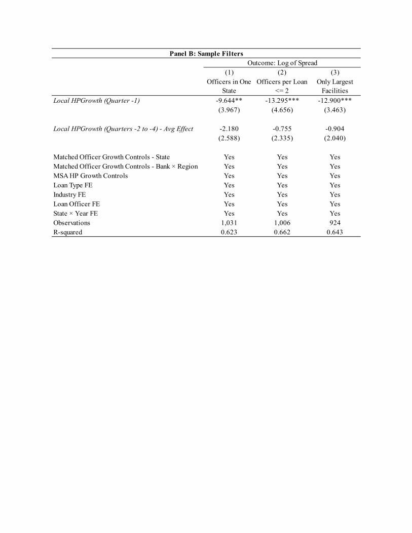
(1) (2) (3)Officers in One

StateOfficers per Loan

<= 2Only Largest

Facilities

Local HPGrowth (Quarter -1) -9.644** -13.295*** -12.900***(3.967) (4.656) (3.463)

Local HPGrowth (Quarters -2 to -4) - Avg Effect -2.180 -0.755 -0.904(2.588) (2.335) (2.040)

Matched Officer Growth Controls - State Yes Yes YesMatched Officer Growth Controls - Bank × Region Yes Yes YesMSA HP Growth Controls Yes Yes YesLoan Type FE Yes Yes YesIndustry FE Yes Yes YesLoan Officer FE Yes Yes YesState × Year FE Yes Yes YesObservations 1,031 1,006 924R-squared 0.623 0.662 0.643

Outcome: Log of SpreadPanel B: Sample Filters

(1) (2) (3) (4) (5) (6) (7) (8) (9) (10)

Outcome:

10 Miles Radius

20 Miles Radius

10 Miles Radius

20 Miles Radius

10 Miles Radius

20 Miles Radius

10 Miles Radius

20 Miles Radius

10 Miles Radius

20 Miles Radius

Local HPGrowth (Quarter -1) 2.181 1.953 64.732 34.092 -0.616 -4.543 -2.678 -4.520 0.031 0.336

(4.006) (5.647) (80.292) (105.618) (2.227) (3.554) (4.278) (6.890) (1.961) (3.585)

Matched Officer Growth Controls - State Yes Yes Yes Yes Yes Yes Yes Yes Yes Yes

Matched Officer Growth Controls - Bank × Region Yes Yes Yes Yes Yes Yes Yes Yes Yes Yes

MSA HP Growth Controls Yes Yes Yes Yes Yes Yes Yes Yes Yes Yes

Loan Type FE Yes Yes Yes Yes Yes Yes Yes Yes Yes Yes

Industry FE Yes Yes Yes Yes Yes Yes Yes Yes Yes Yes

Loan Officer FE Yes Yes Yes Yes Yes Yes Yes Yes Yes Yes

State × Year FE Yes Yes Yes Yes Yes Yes Yes Yes Yes Yes

Observations 1,500 1,316 1,500 1,316 1,099 961 1,500 1,316 1,500 1,316

R-squared 0.397 0.432 0.324 0.347 0.410 0.419 0.484 0.470 0.313 0.326

Additional Loan-Level OutcomesTable IA.14

Log(FacilityAmount) Log(Maturity)

Panel A: Effect of Local Housing Price Growth

Log(LoanShare) %LoanShare Strictness

This table presents our main results with alternative (non-pricing) loan-level outcomes as the dependent variable. Log(LoanShare) is the log of share of theofficer's bank (lead arranger) in the loan. %LoanShare is the share of the officer's bank (lead arranger) in the loan (in percentage points). When loan shareretained by the bank is missing, we impute it based on the loan syndication structure (see text). Strictness represents covenant strictness, computed followingMurfin (2012). Log(FacilityAmount) is the log of loan amount (in millions). Log(Maturity) is the log of loan maturity (in months). Panel A reports the averageeffects of officer local economic experiences (columns (1) and (2) in Panel A of Table 2). Panel B estimates interactive effect of officer local housing pricegrowth and the relevance of borrowers’ real estate value (column (6) in Panel A of Table 6). Standard errors are heteroskedasticity robust and double clusteredby officer and borrower. We report the standard error for each estimate inside brackets. *, **, and *** indicate statistical significance at the 10%, 5%, and 1%,respectively.

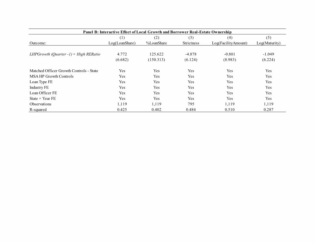
(1) (2) (3) (4) (5)Outcome: Log(LoanShare) %LoanShare Strictness Log(FacilityAmount) Log(Maturity)

LHPGrowth (Quarter -1) × High RERatio 4.772 125.622 -4.878 -0.801 -1.049(6.682) (150.313) (6.124) (8.983) (6.224)

Matched Officer Growth Controls - State Yes Yes Yes Yes YesMSA HP Growth Controls Yes Yes Yes Yes YesLoan Type FE Yes Yes Yes Yes YesIndustry FE Yes Yes Yes Yes YesLoan Officer FE Yes Yes Yes Yes YesState × Year FE Yes Yes Yes Yes YesObservations 1,119 1,119 795 1,119 1,119R-squared 0.425 0.402 0.484 0.510 0.287

Panel B: Interactive Effect of Local Growth and Borrower Real-Estate Ownership

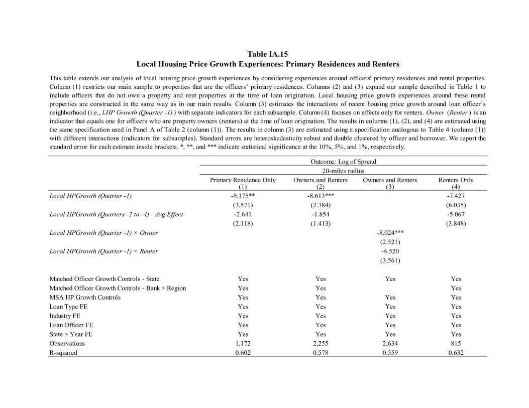
Primary Residence Only Owners and Renters Owners and Renters Renters Only(1) (2) (3) (4)

Local HPGrowth (Quarter -1) -9.175** -8.613*** -7.427

(3.571) (2.384) (6.035)

Local HPGrowth (Quarters -2 to -4) - Avg Effect -2.641 -1.854 -5.067

(2.118) (1.413) (3.848)

Local HPGrowth (Quarter -1) × Owner -8.024***

(2.521)

Local HPGrowth (Quarter -1) × Renter -4.520

(3.561)


Matched Officer Growth Controls - Bank × Region Yes Yes Yes





State × Year FE Yes Yes Yes Yes

Observations 1,172 2,255 2,634 815

R-squared 0.602 0.578 0.559 0.632


Table IA.15Local Housing Price Growth Experiences: Primary Residences and Renters

This table extends our analysis of local housing price growth experiences by considering experiences around officers' primary residences and rental properties.Column (1) restricts our main sample to properties that are the officers’ primary residences. Columns (2) and (3) expand our sample described in Table 1 toinclude officers that do not own a property and rent properties at the time of loan origination. Local housing price growth experiences around these rentalproperties are constructed in the same way as in our main results. Column (3) estimates the interactions of recent housing price growth around loan officer’sneighborhood (i.e., LHP Growth (Quarter -1) ) with separate indicators for each subsample. Column (4) focuses on effects only for renters. Owner (Renter ) is anindicator that equals one for officers who are property owners (renters) at the time of loan origination. The results in columns (1), (2), and (4) are estimated usingthe same specification used in Panel A of Table 2 (column (1)). The results in column (3) are estimated using a specification analogous to Table 4 (column (1))with different interactions (indicators for subsamples). Standard errors are heteroskedasticity robust and double clustered by officer and borrower. We report thestandard error for each estimate inside brackets. *, **, and *** indicate statistical significance at the 10%, 5%, and 1%, respectively.

20-miles radius

Internet Appendix for “Loan Spreads and Credit Cycles: The ...

Documents

Transcript of Internet Appendix for “Loan Spreads and Credit Cycles: The ...