InternationalIlliquidity - phd-finance.uzh.ch4a2b68eb-da0f-4bf3... · In this paper, we study the...

International Illiquidity∗

Aytek MalkhozovBIS†

Philippe MuellerLSE‡

Andrea Vedolin

LSE§

Gyuri Venter

CBS¶

Abstract

We build a parsimonious international asset pricing model in which devia-tions of government bond yields from a fitted yield curve of a country measurethe tightness of investors’ capital constraints. We compute these measuresat daily frequency for six major markets and use them to test the model-predicted effect of funding conditions on asset prices internationally. Globalilliquidity lowers the slope and increases the intercept of the internationalsecurity market line. Local illiquidity helps explain the variation in alphas,Sharpe ratios, and the performance of betting-against-beta (BAB) strategiesacross countries.

Keywords: Liquidity, Margins, Capital Constraints, International CAPM

This Version: April 2016

∗We would like to thank Ines Chaieb, Mathijs Cosemans, Darrell Duffie, Bernard Dumas, VihangErrunza, Jean-Sebastien Fontaine, Sermin Gungor, Peter Kondor, Semyon Malamud, Loriano Mancini,Lasse Pedersen, Giovanni Puopolo, Angelo Ranaldo, Ioanid Rosu, Sergei Sarkissian, Elvira Sojli, andseminar and conference participants at the Banque de France, Bank for International Settlements,Copenhagen Business School, ESMT Berlin, Gaidar Institute Moscow, HEC Lausanne/EPFL, INSEAD,Instituto de Empresa Madrid, McGill University, University of Bern, University of Piraeus, Universityof St. Gallen, the 2014 Asset Pricing Retreat (Tilburg), the 2014 Bank of Canada–Bank of Spain Con-ference (Madrid), the 2014 Mathematical Finance Days, the 2014 CFCM Conference, the 2014 ArneRyde Workshop (Lund), Imperial Conference in International Finance, Asset Pricing Workshop (York),SED Toronto, Dauphine-Amundi Chair Conference (Paris), the 2014 Central Bank Conference on Mar-ket Microstructure (Rome), SAFE Asset Pricing Workshop (Frankfurt), the 2015 Econometric SocietyWinter Meeting (Boston), and the 2015 European Finance Association Annual Meeting (Vienna), theLiquidity Risk in Asset Management Conference (Toronto), INQUIRE Europe (Athens), and the 6thAnnual Financial Market Liquidity Conference (Budapest) for useful comments. Venter gratefully ac-knowledges financial support from the Center for Financial Frictions (FRIC) (grant no. DNRF-102)and the Danish Council for Independent Research (grant no. DFF-4091-00247). All authors thank theDauphine Amundi Chair for financial support.

†Monetary and Economic Department, Email: [email protected]‡Department of Finance, Email: [email protected]§Department of Finance, Email: [email protected]¶Department of Finance, Email: [email protected]

mailto:[email protected]




The recent financial crisis has dramatically illustrated how market frictions can im-

pede orderly investment activity and have significant effects on asset prices.1 These

phenomena are even more prominent when looking at asset prices in an international

context where specialized institutions, such as hedge funds and investment banks, are

responsible for a large fraction of active cross-country investments. In order to under-

stand the specific mechanisms at work and to test various friction-based asset pricing

theories, researchers and policymakers alike require economically-motivated indicators

of market stress.

In this paper, we study the effect of frictions, such as funding constraints or barriers

that impede smooth cross-border movement of capital, on asset prices internationally.

We generically refer to the tightness of these frictions as illiquidity. Our contribution to

the existing literature is threefold. First, we develop a parsimonious international asset

pricing model with constrained investors who trade in equity and bond markets globally.

Second, we construct model-implied proxies for country-level and global illiquidity from

daily bond market data of six developed countries. Third, in line with the model pre-

dictions, we find that global illiquidity affects the international risk-return trade-off by

lowering the slope and increasing the intercept of the international security market line,

stocks in countries with higher local illiquidity earn higher alphas and Sharpe ratios,

and, as a result, accounting for the cross-country differences in illiquidity improves on

the performance of traditional betting-against-beta (BAB) type strategies.

We measure illiquidity as the average squared deviation of observed government

bond prices from those implied by a smooth fitted yield curve. This approach has been

proposed by Hu, Pan, and Wang (2013), who argue that “noise” in the US Treasury

yield curve contains a strong signal about the general scarcity of investment capital

in financial markets. Government bonds are particularly well suited in this context

because they are among the safest and most liquid assets, they are actively traded for

investment purposes, and they are used as the main source of collateral to obtain funding.

Moreover, their prices are known to be well described by a simple factor structure during

normal times. In our model bond price deviations emerge in equilibrium because capital

1See, e.g., Brunnermeier and Pedersen (2009), Garleanu and Pedersen (2011), and He and Krishna-murthy (2012, 2013).

1

constraints prevent investors from eliminating price discrepancies between bonds with

similar risk; larger deviations indicate tighter capital constraints.

Frictions in financial markets can arise for a variety of reasons, such as regulatory

capital requirements, restricted borrowing, margins, investment taxes, or endowment

shocks, all with a similar effect of constraining investment activity.2 In our model, we

assume that investors have to fund a fraction of their position in each asset with their

own capital. We focus on the differential impact of these frictions across countries.

In an international context, more capital may be required to invest in some countries

relative to others, and it may be costly for investors to move capital across borders.

When this constraint binds for at least some investors, the equilibrium expected excess

return on any security depends not only on its risk (e.g., duration for bonds or market

beta for stocks), but also on an additional illiquidity component that is proportional

to the capital required to maintain the position in this asset. Therefore, in the model,

equilibrium bond price deviations are associated with distortions in the relation between

risk and return of other securities, too.

We compute daily illiquidity measures for the US, Germany, the UK, Canada, Japan,

and Switzerland. Unlike other funding liquidity and market stress proxies that suffer

from short time series (e.g., implied volatility indices such as the VIX), are only available

at very low frequency (e.g., broker-dealers’ leverage), or are difficult to compare interna-

tionally (e.g., TED spread), our indicators have the same economic interpretation across

all countries and are available daily for a history of more than 20 years. In terms of

economic magnitude, bond price deviations are a multiple larger than government bond

bid-ask spreads, in particular during crisis periods.

2See, e.g., Black (1972), Frazzini and Pedersen (2013), Stulz (1981), and Vayanos and Wang (2012)for examples of the latter four, respectively. Banking sector investors are subject to non risk-basedcapital requirements under the original Basel and Basel III Leverage Ratio regulations. The newBasel III accord also introduces global liquidity standards (in addition to capital requirements) aimingat improving banks’ liquidity management during periods of high market distress; see, e.g., Strahan(2012). Historically, one famous example is the default of Carlyle Capital Corporation, a large hedgefund which went into bankruptcy on March 5, 2008, after failing to meet several margin calls on theirUSD 22bn fixed income portfolio, which quickly depleted its liquidity. Similarly, during the week ofAugust 6, 2007, a number of quantitative long/short equity hedge funds experienced unprecedentedlosses triggered by a series of margin calls which led to fire sales and additional liquidity shocks acrossdifferent trading strategies; see, e.g., Khandani and Lo (2007).

2

Interestingly, we find that while local illiquidity measures feature a strong common

component, these measures also exhibit significant idiosyncratic variation that is not

shared globally, with countries regularly moving in and out of the more illiquid group.

For example, a major increase in the German and UK indicators following the British

Pound withdrawal from the Exchange Rate Mechanism in September 1992 leaves the

US measure largely unaffected. This provides us with more power to test the impact

of illiquidity on asset returns, exploiting both its global effect and, importantly, its

differences across countries.

Starting with the global effect, the theory predicts that higher average illiquidity

across countries implies a higher intercept and a lower slope of the average international

security market line (SML). This happens because capital-constrained investors value

securities with higher exposure to the global market factor. We find strong support for

this prediction of the model in international stock returns data. For instance, comparing

the lowest to the highest illiquidity quintile, the intercept rises from 0.19% to 0.51% per

month (their difference is statistically different from zero with a t-statistic of 1.77), while

the slope flattens from 0.17% to 0.01% (the difference has a t-statistic of 3.71). When

we control for other determinants of the SML, such as the size or book-to-market factor,

we find the results to remain qualitatively the same.

The theory also predicts that cross-country differences in illiquidity imply a difference

in risk-adjusted returns that compensates investors for the capital they have to commit

to maintain their positions. More precisely, holding the beta of a security constant,

its alpha increases in local illiquidity. We verify this pattern in the cross-section of

illiquidity- and beta-sorted portfolios of international stocks. For example, for high beta

stocks, the alpha increases from 0.40% to 0.52% per month from low to high illiquidity

stocks, the difference which is 0.13% is statistically different from zero with a t-statistic

of 1.97. Similarly, the annualized Sharpe ratio jumps from 0.28 to 0.37.

We proceed to test this implication further by looking at the performance of self-

financing market-neutral portfolios that are constructed to take advantage of the illiq-

uidity alpha.3 First, betting-against-beta (BAB) strategies that exploit constrained

3These strategies would represent a genuine trading opportunity only for unconstrained investorswho do not require a compensation for the shadow cost of the capital constraint.

3

investors’ preference for high-beta assets should perform significantly better in more

illiquid countries. We verify that the portfolio implementing the BAB strategy in coun-

tries that have high illiquidity in a given period outperforms the portfolio doing the

same in low illiquidity countries by 0.74% per month with an associated t-statistic of

4.48. Second, a trading strategy that is long high illiquidity-to-beta-ratio stocks and

short low illiquidity-to-beta-ratio stocks globally (betting-against-illiquidity, or BAIL)

outperforms the global BAB strategy that does not take the difference in illiquidity

across countries into account.

Since funding conditions could be correlated with market illiquidity, we control for

the effect of the latter by orthogonalizing our illiquidity indicators with respect to the

Amihud (2002) stock market illiquidity measure.4 Using the orthogonalized indicators,

we find our theoretical predictions still confirmed in the data.

There exists a large theoretical literature that studies how funding constraints affect

asset prices. Our work is closest to Garleanu and Pedersen (2011) and Frazzini and

Pedersen (2013). Garleanu and Pedersen (2011) show that deviations of the Law of One

Price can arise between assets with the same cash flows but different margins. Frazzini

and Pedersen (2013) model an economy where margin-constrained agents invest in more

risky assets which causes their returns to decline and explains the performance of the

betting-against-beta strategy. Relative to these two papers, we build an international

asset pricing model that motivates our use of a novel country- and global measure of

the tightness of funding constraints and in which the effect of these constraints on asset

prices can be different across countries.

Our work also speaks to Miranda-Agrippino and Rey (2015) who argue that a global

factor related to the constraints of leveraged global banks and asset managers explains

the high degree of international stock return comovement. Relative to their work, we

measure and study the asset pricing implications of both the global level of illiquidity

and its differences across countries.

4For a theoretical link between funding and market liquidity, see, e.g., Brunnermeier and Pedersen(2009). For the US stock market, Chen and Lu (2015) find correlations of 17% to 24% between theirmeasure of funding conditions and various market liquidity proxies.

4

Karolyi, Lee, and van Dijk (2012) study commonality in market liquidity for 40

different stock markets and ask whether the time variation in commonality is mainly

driven by liquidity supply by financial intermediaries or liquidity demand by institutional

investors. Similar to these authors, we do not find a very strong link between market

liquidity and funding conditions. Our contribution shows that funding conditions have

an important effect on international stock returns, even after controlling for market

liquidity.

This paper is also related to several other papers that study liquidity in an interna-

tional context. Amihud, Hameed, Kang, and Zhang (2015) measure market illiquidity

premia in 45 different countries and find that a portfolio long illiquid stocks and short

liquid stocks earns more than 9% per year even when controlling for different global

risk factors. Goyenko and Sarkissian (2014) show that market liquidity of US Treasuries

predicts global stock returns. Bekaert, Harvey, and Lundblad (2007) investigate dif-

ferent definitions of liquidity risk and assess their pricing ability for emerging market

portfolios. Motivated by Acharya and Pedersen (2005), Bekaert, Harvey, and Lundblad

(2007) and Lee (2011) study how liquidity risk is priced in the cross-section of different

stock returns. Different from these papers, we focus on funding illiquidity, for which we

construct new measures, and study its direct effect on expected returns, rather than its

role as a risk factor.

The rest of the paper is organized as follows. Section 1 describes the model and

derives its predictions. Section 2 describes the data and the construction of the illiq-

uidity proxies. Section 3 analyzes the illiquidity measures, while Section 4 presents our

empirical results. Finally, Section 5 concludes. All proofs are deferred to the Appendix.

Additional results are available in an Online Appendix.

1 Model

In this section we build a parsimonous international asset pricing model to guide our

empirical analysis. Throughout the rest of the paper, we index time by t, investors by

i, countries by j, stocks by k, and bonds by h. To simplify the notation, we assume the

5

information about the corresponding country is already contained in indices k and h,

and hence only emphasize the country index j when it is explicitly needed.

1.1 Assumptions

Assets. Time is continuous and goes from zero to infinity. Uncertainty is represented

by a filtered probability space (Ω,F , Ft ,P), on which is defined a standard (N + 1)-

dimensional Brownian motion(Br,t, B

⊤t ≡ (Bt,1, Bt,2, ..., Bt,N)

)⊤, t ∈ [0,∞), with Br,t

being independent of Bt.

We consider a world economy with a set of countries J . In each country j ∈ J there

exist a set of stocks k ∈ Kj and a set of zero-coupon bonds h ∈ Hj as financial assets. We

denote the set of all stocks by K ≡ ∪j∈JKj and the set of all bonds by H ≡ ∪j∈JHj. At

date t, stock k ∈ K is in supply θkt > 0, pays a dividend Dkt in the unique consumption

good, which we assume to be driven by Bt, and its ex-dividend price is denoted by P kt .

Bonds are assumed to be in zero net supply. For each h ∈ H, we denote the time t

price of the zero-coupon bond h paying one dollar at maturity t+ τh by Λht , and its yield

by yht = − 1τhlog Λh

t . Agents also have access to a global riskless asset with instantaneous

return (i.e., short rate) rt given exogenously, only driven by Br,t.5 Finally, we assume

that purchasing power parity holds and all prices are expressed in US dollars.

Agents. Stocks and bonds are held by two types of investors: buy-and-hold agents and

optimizing financial institutions. We assume that buy-and-hold agents have exogenously

given demand dht for bond h at time t, and do not trade stocks. We understand them

as the source of the net supply of bonds coming from the domestic and international

official sector, preferred-habitat investors, or noise traders.6

Financial institutions are competitive and have mean-variance preferences over the

instantaneous change in the value of their portfolios. We have in mind investors such

5The independence assumption on Br,t and Bt is to simplify our derivation, and can be relaxedwithout qualitative changes to our results. The assumption that the short rate rt only depends ona one-dimensional Brownian motion implies that bond yields in the model have one common factor.The model could easily accommodate several (e.g., three) yield factors, without adding any additionaleconomic message to our framework.

6These agents play a role similar to preferred-habitat investors in the term structure model of Vayanosand Vila (2009). Similar to that paper, we could allow buy-and-hold agents to have a downward-slopingdemand curve for bonds, but this would not change qualitatively our results.

6

as investment banks, hedge funds, and fund managers, who trade actively in the inter-

national stock and bond markets, and act as marginal investors there in the short- to

medium-run. In short, we refer to them as investors.

Investor i ∈ I, born with wealth Wi,t ≥ 0, can invest in all assets of the world

economy. If xki,t and zhi,t denote the dollar amount investor i holds in stock k and bond

h at time t, respectively, her budget constraint is

dWi,t =

Wi,t −

∫

k∈K

xki,tdk −

∫

h∈H

zhi,tdh

rtdt+

∫

k∈K

xki,tDk

t dt+ dP kt

P kt

dk +

∫

h∈H

zhi,tdΛh

t

Λht

dh.

(1)

We further assume that investor i’s portfolio holdings in risky securities, which include

all stocks and bonds, have to satisfy the following constraint:

∫

k∈K

mki,t

∣∣xki,t

∣∣ dk +

∫

h∈H

mhi,t

∣∣zhi,t∣∣ dh ≤Wi,t. (2)

The constraint implies that investing in or shorting securities requires investor i to

commit the amount of her capital equal to the multiple mki,t (or m

hi,t) of the position

size. Thus, investor i maximizes the mean-variance objective

maxxk

i,tk∈K,zhi,th∈H

Et [dWi,t]−α

2Vart [dWi,t] (3)

subject to (2), where α is her risk-aversion coefficient.

1.2 Equilibrium

We write stock and bond price dynamics in the forms

dP kt =

(µkP,tP

kt −Dk

t

)dt+ P k

t σk⊤P,tdBt (4)

and

dΛht = Λh

t

(µhΛ,tdt− σh

Λ,tdBr,t

), (5)

7

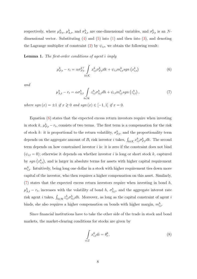
respectively, where µkP,t, µ

hΛ,t, and σ

hΛ,t are one-dimensional variables, and σk

P,t is an N -

dimensional vector. Substituting (4) and (5) into (1) and then into (3), and denoting

the Lagrange multiplier of constraint (2) by ψi,t, we obtain the following result:

Lemma 1. The first-order conditions of agent i imply

µkP,t − rt = ασk⊤

P,t

∫

k∈K

xki,tσkP,tdk + ψi,tm

ki,tsgn

(xki,t)

(6)

and

µhΛ,t − rt = ασh

Λ,t

∫

h∈H

zhi,tσhΛ,tdh+ ψi,tm

hi,tsgn

(zhi,t), (7)

where sgn (x) = ±1 if x ≷ 0 and sgn (x) ∈ [−1, 1] if x = 0.

Equation (6) states that the expected excess return investors require when investing

in stock k, µkP,t − rt, consists of two terms. The first term is a compensation for the risk

of stock k: it is proportional to the return volatility, σkP,t, and the proportionality term

depends on the aggregate amount of Bt risk investor i takes,∫

k∈Kxki,tσ

kP,tdk. The second

term depends on how constrained investor i is: it is zero if the constraint does not bind

(ψi,t = 0); otherwise it depends on whether investor i is long or short stock k, captured

by sgn(xki,t), and is larger in absolute terms for assets with higher capital requirement

mki,t. Intuitively, being long one dollar in a stock with higher requirement ties down more

capital of the investor, who then requires a higher compensation on this asset. Similarly,

(7) states that the expected excess return investors require when investing in bond h,

µhΛ,t − rt, increases with the volatility of bond h, σh

Λ,t, and the aggregate interest rate

risk agent i takes,∫

h∈Hzhi,tσ

hΛ,tdh. Moreover, as long as the capital constraint of agent i

binds, she also requires a higher compensation on bonds with higher margin, mhi,t.

Since financial institutions have to take the other side of the trade in stock and bond

markets, the market-clearing conditions for stocks are given by

∫

i∈I

xki,tdi = θkt , (8)

8

and for bonds by∫

i∈I

zhi,t + dht = 0, (9)

for all t, k, and h.

Aggregating (6) across all investors i ∈ I and imposing market-clearing condition

(8), we get

µkP,t − rt = ασk⊤

P,t

∫

k∈K

θkt σkP,tdk +

∫

i∈I

ψi,tmki,tsgn

(xki,t)di. (10)

Let us define a global market index, Gt, that is the dollar-supply weighted average of all

stocks; the value and the dynamics of this global index, respectively, are given by

Gt =

∫

k∈K

θkt dk and dGt =

∫

k∈K

θktDk

t dt+ dP kt

P kt

dk. (11)

Combining (10) and (11), after some algebra, we obtain the following result:

Theorem 1. The equilibrium expected excess return of security k is

µkP,t − rt = βk

P,tλt + φkt − βk

P,tφGt , (12)

with

φkt =

∫

i∈I

ψi,tmki,tsgn

(xki,t)di and φG

t =

∫

k∈K

φkt

θkt∫

k∈K

θkt dkdk, (13)

where βkP,t = Covt

[Dk

t dt+dP kt

P kt

, dGt

Gt

]

/Vart

[dGt

Gt

]

is the beta of security k returns with respect

to the global market portfolio return, and λt = µG,t − rt is the expected excess return of

the global market portfolio.7

7The term φGt appears in (12) because excess returns on the global market portfolio are themselvesin part driven by the compensation for the constraint.

9

Next we look at the equilibrium prices of bonds.8 As in the case of stocks, aggregating

(7) across all investors i ∈ I and imposing market-clearing condition (9), we obtain:

µhΛ,t − rt = −ασh

Λ,t

∫

h∈H

dht σhΛ,tdh+

∫

i∈I

ψi,tmhi,tsgn

(zhi,t)di. (14)

In the Appendix we characterize zero-coupon bond prices in the general case, derived

from (14) without further assumptions. For the purpose of this paper, however, it is

more illustrative to consider a special case in which a closed-form solution is available:

Theorem 2. Suppose the dynamics of the short rate rt under the physical probability

measure are given by the mean-reverting process

drt = κ (r − rt) dt+ σdBr,t,

where κ, r, and σ are all positive constants. Moreover, suppose that mhi,t, d

ht , m

ki,t, θ

kt ,

and Wi,t are constant over time but can vary across investors and assets. Then the

equilibrium yield on bond h is given by

yht = A (τh) + B (τh) rt + Ch (τh) ,

where the first two terms describe a standard affine yield curve that depends only on the

maturity of a bond and the short-rate factor rt, and

Ch (τh) =1

τh

∫

h′<h

∫

i∈I

ψi,tmh′

i,tsgn(

zt+τh′i,t

)

didh′ (15)

represents a deviation from this smooth yield curve, specific to bond h.9

8Due to the assumptions, our setting allows us to discuss stock and bond pricing separately, but itcould easily accommodate a non-zero correlation between the risk of stocks and bonds. In this case,the combined stock and bond global portfolio becomes the relevant market portfolio. Zero correlationallows us to follow Frazzini and Pedersen (2013), who use asset-class-specific market portfolios. In eithercase, qualitative predictions regarding the effect of illiquidity on excess returns are the same.

9In the general case, when fundamentals are not constant over time, Ch (τh) depends on the currentand expected future values of ψi,t, m

hi,t, and sgn

(zt+τhi,t

); see Lemma 2 of the Appendix.

10

1.3 Discussion and Predictions

The model above provides us with a minimal setting that introduces a friction into

investors’ myopic risk-return tradeoff in both stock and bond markets. The friction

takes the form of a capital constraint similar to Garleanu and Pedersen (2011), He and

Krishnamurthy (2012), and Frazzini and Pedersen (2013).10

Our focus is on the effect of such constraints at the country level. In the model,

illiquidity conditions can differ across countries for two reasons. Capital requirements

mki,t and m

hi,t are asset- and investor-specific. In particular, they have a country-specific

component and can be higher for foreign investors. In the latter case, a constrained

investor located in a given country will have a different effect on the illiquidity component

of expected returns domestically and internationally, as can be seen from (10) and (14).

Cross-border flows may require more capital because such investments involve a higher

degree of intermediation. Also, the effect of higher cross-border capital requirements

is isomorphic to that of barriers to international investments studied in Stulz (1981),

Bhamra, Coeurdacier, and Guibaud (2014), and Garleanu, Panageas, and Yu (2015).11

We abstract away from exchange rate risk by imposing purchasing power parity;

see, e.g., Bekaert, Harvey, and Lundblad (2007) who make a similar assumption. Thus,

from investors’ perspective, countries differ only in the capital required to fund posi-

tions there. In practice, however, the costs of hedging in foreign exchange markets

and exchange rate movements themselves can also depend on funding conditions (see,

e.g., Ivashina, Scharfstein, and Stein (2015) and Mancini, Ranaldo, and Wrampelmeyer

(2013), respectively), and thus could be indirectly captured in our analysis.

Based on Theorems 1 and 2, we derive five predictions that link illiquidity phenomena

in international bond and stock markets. First, noise in the yield curve is informative

about illiquidity conditions in a given country.

10A model with non-myopic agents can deliver further predictions: In addition to taking the currentcapital constraint into account in their optimization, investors will want to hedge against the futurestates where the constraint will bind; see, e.g., Kondor and Vayanos (2015) and Malamud and Vilkov(2015). Testing whether international illiquidity, in addition to its myopic effect on asset returns, isalso a priced risk factor is an interesting extension that we leave for future research.

11At the same time, our setting is different from the market segmentation model of Errunza and Losq(1985), where foreign investors are prohibited from taking any position in a subset of domestic stocks.

11

Proposition 1. In each country there exists a smooth theoretical yield curve, but bond

yields can be off the curve. Everything else being equal, deviations are larger in countries

where investors are more constrained, i.e., illiquidity is higher.

Proposition 1 follows from Theorem 2. In particular, (15) shows that the deviation

of bond h from a standard affine yield curve depends on the capital required to invest in

this bond and the position (long or short) that investors take in it. For instance, bonds

for which buy-and-hold investors have a short (long) net position will tend to be more

expensive (cheap) compared to the frictionless benchmark yield curve to compensate

constrained investors for the capital they have to commit to take the other side of the

trade.12 Everything else being equal, the average magnitude of such deviations across all

bonds in country j is higher if it is more difficult to fund positions in this country, and

if investors are more constrained. We refer to this average effect of capital constraints

at the country level as local illiquidity, and proxy for them by the average yield curve

deviation.

Next, we look at the effect of country-level and average global illiquidity on expected

stock returns. Similarly to the bond market, equation (13) shows that the terms φkt

capturing the effect of constraints on stock returns depend on capital requirements and

shadow prices of capital ψi,t. Because constrained investors trade in both stocks and

bonds, the latter are the same in both markets. In addition, we think of capital re-

quirements as having a country-level component that affects the funding of positions in

all securities in a given country. Thus, φkt is related to our local illiquidity indicators,

derived from bond yields, while φGt to their global average.

Proposition 2. There is an average global security market line (SML) with slope de-

creasing in global illiquidity and intercept increasing in global illiquidity.

Proposition 2 is a simple rearrangement of (12) in Theorem 1:

µkP,t − rt = φG

t︸︷︷︸

average intercept

+βkt

(λt − φG

t

)

︸︷︷︸

slope of SML

+(φkt − φG

t

)

︸︷︷︸

country effect

,

12For instance, as reported in the FR 2004 statistical reports by the Federal Reserve Bank of NewYork, primary dealers in the US Treasuries market hold long positions in some maturities and shortpositions in others.

12

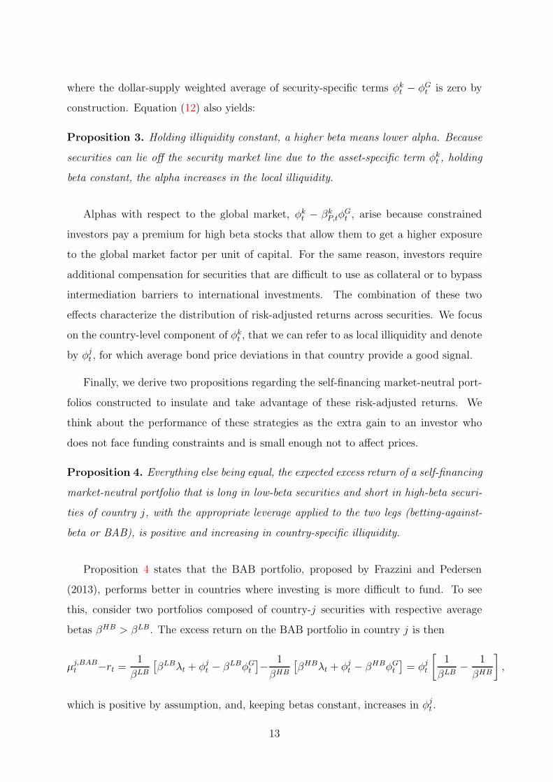
where the dollar-supply weighted average of security-specific terms φkt − φG

t is zero by

construction. Equation (12) also yields:

Proposition 3. Holding illiquidity constant, a higher beta means lower alpha. Because

securities can lie off the security market line due to the asset-specific term φkt , holding

beta constant, the alpha increases in the local illiquidity.

Alphas with respect to the global market, φkt − βk

P,tφGt , arise because constrained

investors pay a premium for high beta stocks that allow them to get a higher exposure

to the global market factor per unit of capital. For the same reason, investors require

additional compensation for securities that are difficult to use as collateral or to bypass

intermediation barriers to international investments. The combination of these two

effects characterize the distribution of risk-adjusted returns across securities. We focus

on the country-level component of φkt , that we can refer to as local illiquidity and denote

by φjt , for which average bond price deviations in that country provide a good signal.

Finally, we derive two propositions regarding the self-financing market-neutral port-

folios constructed to insulate and take advantage of these risk-adjusted returns. We

think about the performance of these strategies as the extra gain to an investor who

does not face funding constraints and is small enough not to affect prices.

Proposition 4. Everything else being equal, the expected excess return of a self-financing

market-neutral portfolio that is long in low-beta securities and short in high-beta securi-

ties of country j, with the appropriate leverage applied to the two legs (betting-against-

beta or BAB), is positive and increasing in country-specific illiquidity.

Proposition 4 states that the BAB portfolio, proposed by Frazzini and Pedersen

(2013), performs better in countries where investing is more difficult to fund. To see

this, consider two portfolios composed of country-j securities with respective average

betas βHB > βLB. The excess return on the BAB portfolio in country j is then

µj,BABt −rt =

1

βLB

[βLBλt + φj

t − βLBφGt

]−

1

βHB

[βHBλt + φj

t − βHBφGt

]= φj

t

[1

βLB−

1

βHB

]

,

which is positive by assumption, and, keeping betas constant, increases in φjt .

13

Proposition 5. The expected excess return of a self-financing market-neutral portfolio

that is long in high illiquidity-to-beta ratio securities and short in low illiquidity-to-

beta ratio securities (betting-against-illiquidity or BAIL) is positive and higher than the

expected return on a similar long-short trading strategy that ignores sorting on illiquidity.

Proposition 5 states that taking into account the difference in country-level illiquidity

could improve on the performance of the global BAB portfolio. Formally, consider two

global portfolios with respective average betas βH and βL and illiquidities φHt and φL

t .

Creating a long-short portfolio of them, in which the leverage applied to the two legs

are inversely proportional to betas, has an excess return of

µH−Lt − rt =

1

βH

[βHλt + φH

t − βHφGt

]−

1

βL

[βLλt + φL

t − βLφGt

]=φHt

βH−φLt

βL.

If φHt /β

H > φLt /β

L, the excess return on this risk-neutral BAIL portfolio is positive, and

increases in the difference of the illiquidity-to-beta ratios.

In the following, we take our main model predictions to the data. To this end, we

first introduce model-implied illiquidity proxies for six different countries.

2 Data

In this section we describe our data and the construction of country-level and global

illiquidity measures.

2.1 Bond Data

We collect raw data on government bonds and stock return data from Datastream. The

frequency is daily, running from 1 January 1990 to 31 December 2012, leaving us with

6,001 observations in the time-series.

The bond data spans six different countries: the United States, Germany, the United

Kingdom, Canada, Japan, and Switzerland.13 We obtain a daily cross-section of end-of-

13The country choice is driven by two main factors: data availability and credit risk considerations.For example, while there is enough data available on some Eurozone countries, these sovereign bondsfeature quite a large credit risk component, especially after 2008 (see, e.g., Pelizzon, Subrahmanyam,Tomio, and Uno (2016)), an aspect absent from our model.

14

day bond prices for our sample period for all available maturities. We use mid prices to

avoid any discrepancies between the prices of similar bonds due to the bid-ask spread.

Furthermore, we collect information on accrued interest, coupon rates and dates,

and issue and redemption. Following Gurkaynak, Sack, and Wright (2007), we apply

several data filters in order to obtain securities with similar liquidity and avoiding special

features. The filters can vary by country, but in general they are as follows: (i) We

exclude bonds with option like features such as bonds with warrants, floating rate bonds,

callable and index-linked bonds. (ii) We consider only securities with a maturity of more

than one year at issue (this means that, for example, for the US market we exclude

Treasury bills). We also exclude securities that have a remaining maturity of less than

three months to alleviate concerns that segmented markets may significantly affect the

short-end of the yield curve.14 Moreover, short-maturity bonds are not very likely to

be affected by arbitrage activity, which is the objective of our paper. (iii) We exclude

bonds with a remaining maturity of 15 years or more as in an international context

they are often not very actively traded (see, e.g., Pegoraro, Siegel, and Tiozzo ‘Pezzoli’

(2013)). (iv) For the US we exclude the on-the-run and first-off-the-run issues for every

maturity. These securities often trade at a premium to other Treasury securities as

they are generally more liquid than more seasoned securities (see, e.g., Fontaine and

Garcia (2012)). Other countries either do not have on-the-run and off-the-run bonds

in the strict sense, as they for example reopen existing bonds to issue additional debt,

or they do not conduct regular auctions as the US Treasury does. We therefore do not

apply this filter to the international sample. (v) Additionally, we exclude bonds if the

reported prices are obviously wrong. While the data quality for the US is reasonably

good, there are a lot of obvious pricing errors in the international bond sample, which

requires substantial manual data cleaning.

Panel A of Table 1 provides details of our international bond sample. We note

that on average we have 71 bonds every day to fit the yield curve and 60 bonds to

construct the illiquidity measure. Japan and the US are the most active markets, while

the average number of bonds in Switzerland and the UK are lower. The cross-section

14Duffee (1996), for example, shows that Treasury bills exhibit a lot of idiosyncratic variation andhave become increasingly disconnected from the rest of the yield curve.

15

varies considerable over time: During the years 2001 and 2007, the number of bonds

available dropped considerably for all countries except Japan, which was a response to

the banking crisis in the years 2000.

[Insert Table 1 here.]

2.2 Stock Data

To assess the asset pricing implications of our proxies of illiquidity, we collect daily stock

returns, volume, and market capitalization data for the six countries from Datastream.

The initial sample covers more than 10,000 stocks. We only select stocks from major

exchanges, which are defined as those in which the majority of stocks for a given country

are traded. We exclude preferred stocks, depository receipts, real estate investment

trusts, and other financial assets with special features based on the specific Datastream

type classification. To limit the effect of survivorship bias, we include dead stocks in

the sample. We exclude non-trading days, defined as days on which 90% or more of the

stocks that are listed on a given exchange have a return equal to zero. We also exclude

a stock if the number of zero-return days is more than 80% in a given month. Excess

returns are calculated versus the US Treasury bill rate and the proxy for the global

market is the MSCI world index. Panel B of Table 1 reports summary statistics.

We follow Frazzini and Pedersen (2013) to construct ex-ante betas for our dataset

of international stocks from rolling regressions of daily excess returns on market excess

returns. The estimated beta for stock k at time t is given by:

βkt,TS = ρkt

σkt

σGt

,

where σkt and σ

Gt are the estimated volatilities for the stock and the market and ρkt is their

correlation. Volatilities and correlations are estimated separately. First, we use a one-

year rolling standard deviation for volatilities and a five-year horizon for the correlation

to account for the fact that correlations appear to move more slowly than volatilities. To

account for non-synchronous trading, we use one-day log returns to estimate volatilities

16

and three-day log returns for correlation. Finally, we shrink the time-series estimate of

the beta towards the cross-sectional mean (βkt,CS) following Vasicek (1973):

βkt = ωβk

t,TS + (1− ω) βkt,CS,

where we set ω = 0.6 for all periods and all stocks, in line with Frazzini and Pedersen

(2013).

2.3 Country-Level Illiquidity Proxies

To construct country-specific illiquidity measures, we follow Hu, Pan, and Wang (2013)

who employ the Svensson (1994) method to fit the term structure of interest rates.15

The Svensson (1994) model assumes that the instantaneous forward rate is given by

fm,b = β0 + β1exp

(

−m

τ1

)

+ β2m

τ1exp

(

−m

τ1

)

+ β3m

τ2exp

(

−m

τ2

)

,

where m denotes the time to maturity and b = (β0, β1, β2, β3, τ1, τ2) are parameters to be

estimated. By integrating the forward rate curve, we derive the zero-coupon spot curve:

sm,b = β0 + β1

(

1− exp

(

−m

τ1

))(m

τ1

)−1

+β2

((

1− exp

(

−m

τ1

))(m

τ1

)−1

− exp

(

−m

τ1

))

+β3

((

1− exp

(

−m

τ2

))(m

τ2

)−1

− exp

(

−m

τ2

))

.

A proper set of parameter restrictions is given by β0 > 0, β0 + β1 > 0, τ1 > 0, and

τ2 > 0. For long maturities, the spot and forward rates approach asymptotically β0,

hence the value has to be positive. (β0 + β1) determines the starting value of the curve

at maturity zero. (β2, τ1) and (β3, τ2) determine the humps of the forward curve. The

hump’s magnitude is given by the absolute size of β2 and β3 while its direction is given

by the sign. Finally, τ1 and τ2 determine the position of the humps.

15We also use the Nelson and Siegel (1987) and a cubic spline method. All three approaches lead toqualitatively very similar results. We chose the Svensson (1994) method over the other two as it is themost widely used and also the most flexible.

17

To estimate the set of parameters bjt for each country j and day t, we minimize the

weighted sum of the squared deviations between actual and model-implied prices:

bjt = argminb

Hjt∑

h=1

[(P h (b)− P h

t

)×

1

Dht

]2

,

where Hjt denotes the number of bonds available in country j on day t, P h (b) is the

model-implied price for bond h = 1, ..., Hjt , P

ht is its observed bond price, and Dh

t is

the corresponding Macaulay duration. We verify that our yield curve estimates are

reasonable by comparing our term structures with the estimates published by central

banks or the international yield curves used in Wright (2011) and Pegoraro, Siegel, and

Tiozzo ‘Pezzoli’ (2013).16

The illiquidity measure for country j is then defined as the root mean square error

between the model-implied yields and the market yields, i.e.,

Illiqjt =

√√√√ 1

Hjt

Hjt∑

h=1

[yh(bjt)− yht

]2,

where yh(bjt)is the model-implied yield corresponding to bond h and yht is the market

yield.

While we calculate the term structure using a wide range of maturities, we calculate

the measure only using bonds with maturities ranging between one and ten years. Similar

to Hu, Pan, and Wang (2013), we also apply data filters to ensure that the illiquidity

measures are not driven by single observations. In particular, we exclude any bond whose

associated yield is more than four standard deviations away from the model yield.

To get a measure of global illiquidity, we construct a market-capitalization weighted

average of each country-level illiquidity measure in line with our theoretical model pro-

posed in the previous section:

IlliqGt =1

total market cap

6∑

j=1

market capjt × Illiqjt .

16We thank Fulvio Pegoraro and Luca Tiozzo ‘Pezzoli’ for sharing their codes.

18

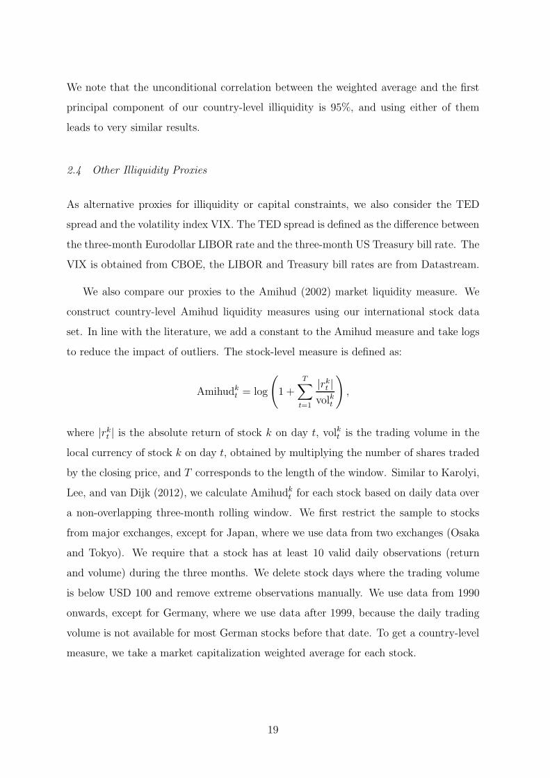
We note that the unconditional correlation between the weighted average and the first

principal component of our country-level illiquidity is 95%, and using either of them

leads to very similar results.

2.4 Other Illiquidity Proxies

As alternative proxies for illiquidity or capital constraints, we also consider the TED

spread and the volatility index VIX. The TED spread is defined as the difference between

the three-month Eurodollar LIBOR rate and the three-month US Treasury bill rate. The

VIX is obtained from CBOE, the LIBOR and Treasury bill rates are from Datastream.

We also compare our proxies to the Amihud (2002) market liquidity measure. We

construct country-level Amihud liquidity measures using our international stock data

set. In line with the literature, we add a constant to the Amihud measure and take logs

to reduce the impact of outliers. The stock-level measure is defined as:

Amihudkt = log

(

1 +

T∑

t=1

|rkt |

volkt

)

,

where |rkt | is the absolute return of stock k on day t, volkt is the trading volume in the

local currency of stock k on day t, obtained by multiplying the number of shares traded

by the closing price, and T corresponds to the length of the window. Similar to Karolyi,

Lee, and van Dijk (2012), we calculate Amihudkt for each stock based on daily data over

a non-overlapping three-month rolling window. We first restrict the sample to stocks

from major exchanges, except for Japan, where we use data from two exchanges (Osaka

and Tokyo). We require that a stock has at least 10 valid daily observations (return

and volume) during the three months. We delete stock days where the trading volume

is below USD 100 and remove extreme observations manually. We use data from 1990

onwards, except for Germany, where we use data after 1999, because the daily trading

volume is not available for most German stocks before that date. To get a country-level

measure, we take a market capitalization weighted average for each stock.

19

3 Illiquidity Facts

In this section we document the key time series and cross-sectional properties of our

illiquidity measures, and compare them to other market stress indicators.

3.1 Properties of Illiquidity

The time-series of all country-specific illiquidity measures, in basis points, are plotted

in Figure 1. In Panel A of Table 2, we report summary statistics. Overall, the average

pricing errors are quite small, ranging from 2.8 basis points (bp) for the US to 6.2 bp

for Switzerland. The larger pricing errors also come with an overall larger volatility that

ranges from 4.5 bp (Switzerland) to 1.37 bp (US). To put the magnitude of these pricing

deviations into economic perspective, we can compare them to the bid-ask spreads. In

the US Treasuries market, for which we have detailed bid-ask spread studies, pricing

errors are larger than the bid-ask spread on average, and in particular are several times

larger during illiquidity spikes. For instance, Engle, Fleming, Ghysels, and Nguyen

(2013) report spreads for five-year Treasuries that do not exceed 1 bp in normal times

and 2 bp at the height of the crisis in 2009.

One might suspect that in the time-series countries which tend to be more illiquid

remain illiquid in the cross-section over long periods of time. To this end, we sort

each country-level illiquidity proxy at the end of each month into three different bins,

depending on their illiquidity: The low (high) illiquidity bin contains the countries which

are in the lowest (highest) tercile of illiquidity. Panel B reports the average fraction of

how many months each country-level illiquidity measure is in the low, medium, or high

bin out of the 276 months (ranging from January 1990 to December 2012). We note

that except for Japan and Switzerland, the frequency of being in either of the three bins

is quite equally distributed for the other four countries. Japan is in the low illiquidity

bin 2/3 of the time, while Switzerland is in the high illiquidity bin 77% of all times.

[Insert Table 2 and Figures 1 and 2 here.]

The time-series variation in country-level illiquidity exhibits significant commonality.

Pairwise correlations between illiquidity proxies reported in Panel C of Table 2 are all

20

positive and range between 20% (US and Japan) and 74% (Germany and Japan). Panel

D of Table 2 reports loadings from the following regression:

Illiqjt = βj0 + βj

1IlliqGt + ǫjt ,

where Illiqjt is the illiquidity proxy of country j and IlliqGt is the global illiquidity proxy.

Unsurprisingly, we find that all country-level measures co-move positively with the global

illiquidity factor, and that the latter explains a significant proportion of the variation

in the country-level illiquidity with R2 ranging between 39% and 66%. We note that

the high unconditional correlation between country-level illiquidities is driven by a few

crisis episodes. Figure 3 plots the average conditional correlation among the different

illiquidity proxies, calculated on daily data using a three-year rolling window. The

average correlation peaks during periods of distress such as the dotcom bubble burst

or the most recent financial crisis where the correlation reaches almost 80%, but is

significantly lower otherwise. We also note an upward trend in the conditional correlation

that could point towards higher market integration.

[Insert Figure 3 here.]

Next, we look at the dispersion of illiquidity across countries. As can be seen from

Table 2, the levels of country-level illiquidity are relatively close on average. In other

words, there are no large permanent differences in illiquidity between the countries we

consider. This is perhaps not surprising given that we include only developed financial

markets in our analysis. However, illiquidity can become significantly dispersed when

some countries experience idiosyncratic illiquidity episodes. Figure 4 illustrates the

cross-sectional standard deviation of illiquidity measures.


Overall, illiquidity exhibits significant country-specific variation: country- or region-

specific events seem to be reflected in spikes in the respective local illiquidity measures

that are not shared globally. For example, the Japanese measure is highly volatile in the

21

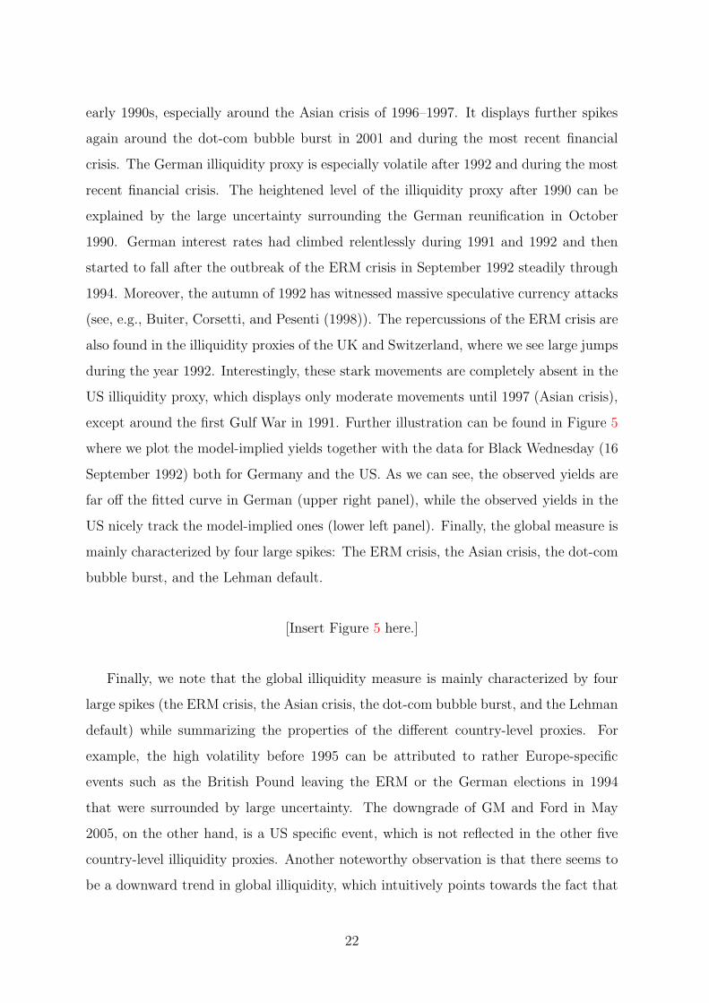
early 1990s, especially around the Asian crisis of 1996–1997. It displays further spikes

again around the dot-com bubble burst in 2001 and during the most recent financial

crisis. The German illiquidity proxy is especially volatile after 1992 and during the most

recent financial crisis. The heightened level of the illiquidity proxy after 1990 can be

explained by the large uncertainty surrounding the German reunification in October

1990. German interest rates had climbed relentlessly during 1991 and 1992 and then

started to fall after the outbreak of the ERM crisis in September 1992 steadily through

1994. Moreover, the autumn of 1992 has witnessed massive speculative currency attacks

(see, e.g., Buiter, Corsetti, and Pesenti (1998)). The repercussions of the ERM crisis are

also found in the illiquidity proxies of the UK and Switzerland, where we see large jumps

during the year 1992. Interestingly, these stark movements are completely absent in the

US illiquidity proxy, which displays only moderate movements until 1997 (Asian crisis),

except around the first Gulf War in 1991. Further illustration can be found in Figure 5

where we plot the model-implied yields together with the data for Black Wednesday (16

September 1992) both for Germany and the US. As we can see, the observed yields are

far off the fitted curve in German (upper right panel), while the observed yields in the

US nicely track the model-implied ones (lower left panel). Finally, the global measure is

mainly characterized by four large spikes: The ERM crisis, the Asian crisis, the dot-com

bubble burst, and the Lehman default.


Finally, we note that the global illiquidity measure is mainly characterized by four

large spikes (the ERM crisis, the Asian crisis, the dot-com bubble burst, and the Lehman

default) while summarizing the properties of the different country-level proxies. For

example, the high volatility before 1995 can be attributed to rather Europe-specific

events such as the British Pound leaving the ERM or the German elections in 1994

that were surrounded by large uncertainty. The downgrade of GM and Ford in May

2005, on the other hand, is a US specific event, which is not reflected in the other five

country-level illiquidity proxies. Another noteworthy observation is that there seems to

be a downward trend in global illiquidity, which intuitively points towards the fact that

22

over time more arbitrage capital has become available and, hence, constraints are less

binding.

3.2 Comparison with Other Illiquidity Measures

In the following, we compare our illiquidity measures to other market stress indicators.

To save space, we report all results in the Online Appendix. As a first measure, we look

at the Amihud measure as it is one of the most widely used proxies of market liquidity.

In Section OA-1 of the Online Appendix, we report that the unconditional correlation

between country-level stock market illiquidity measures constructed following Amihud

(2002) and our illiquidity measures is positive and ranges between 10% (Germany) and

43% (US). The correlation is largely driven by the 2008 period.

There is an intimate link between funding liquidity and market volatility, and the

causality of the relationship can possibly go in either direction.17 Brunnermeier and

Pedersen (2009), among others, suggest the VIX index as a proxy for funding liquidity

itself. In Section OA-2 of the Online Appendix, we compare our illiquidity proxies

with country-level VIX for the longest time-series available.18 We note that overall

the correlation between the time-series is quite high ranging from 49% (Japan) to 66%

(Germany and Switzerland).

In addition, we also test for Granger causality between our illiquidity measures,

Amihud (2002) market illiquidity, and volatility in each country. The results show only

limited evidence for causality linkages between our illiquidity and Amihud market illiq-

uidity, which is perhaps not surprising given the relatively low correlation between them.

17For example, Karolyi, Lee, and van Dijk (2012) find that international illiquidity measures co-move more during periods of high volatility. Hedegaard (2014) finds a large effect from margins ontovolatility in the commodity market. Hardouvelis (1990) and Hardouvelis and Peristiani (1992), onthe other hand, argue that more stringent margins lead to lower stock market volatility in the USand in Japan, respectively. While from a policy perspective it is interesting to study how mar-gins affect volatility, the relationship can also go the opposite direction. For options and futures,margin requirements are set based on volatility itself. For example, the Chicago Mercantile Ex-change (CME) uses the so called SPAN (Standard Portfolio Analysis of Risk) method that calculatesthe maximum likely loss that could be suffered by a portfolio. The method consists of 16 differ-ent scenarios which are comprised of different market prices and volatility. For more informationsee http://www.cmegroup.com/clearing/files/span-methodology.pdf. Similarly, on the LondonStock Exchange, the initial margin is calculated based on the maximum loss according to volatility andinvestors’ leverage.

18We could not find any data on the Canadian equivalent of VIX.

23

We find stronger support for volatility causing both stock market and our illiquidity, as

well as a reverse causality link.

Finally, in Section OA-3 of the Online Appendix, we compare our global proxy with a

range of other illiquidity measures that are not available for countries other than the US.

The unconditional correlation ranges between 4% (Fontaine and Garcia (2012) measure)

and 65% (Goyenko, Subrahmanyam, and Ukhov (2011) proxy).

4 Empirical Results

In this section we use the illiquidity measures to test the predictions of our theory that

assumes investors being capital constrained when forming their optimal portfolio.

4.1 Global Illiquidity and the Security Market Line

Proposition 2 states that the slope of the average SML should depend negatively on the

tightness of global margin constraints, while the intercept is positively related to it. As

a first illustration, we follow the procedure in Cohen, Polk, and Vuolteenaho (2005) and

divide our monthly data sample into quintiles according to the level of global illiquidity.

We then examine the pricing of beta-sorted portfolios in these quintiles and estimate the

empirical SML. Figure 6 depicts the average intercept and slope of the SML for different

levels of global illiquidity ranging from low illiquidity (bin 1) to high illiquidity (bin 5).


We note that in line with our prediction, the slope coefficient is decreasing with

global illiquidity, while the intercept is increasing. For example, for low illiquidity states

the average intercept is 0.191% with a slope of 0.171%, whereas for high illiquidity, the

intercept increases to 0.51% and the slope decreases to 0.008%. The difference between

the low and high illiquidity bin intercept is 0.32% per month which is statistically dif-

ferent from zero with a t-statistic of 1.77. Similarly, the difference in slope coefficients

which is 0.16% is highly statistically different from zero with a t-statistic of 3.71.

24

Next, we study in more detail how the intercept and the slope are affected by global

illiquidity risk. To this end, we consider Fama and MacBeth (1973) regressions and

regress excess returns on the basis assets on a constant and the portfolios’ trailing-

window post-ranking beta:

rxjt = αt + φt × βjt + ǫjt ,

where rxjt is the excess return of the j-th β-sorted portfolio and βjt is the post-ranking

beta of portfolio j. This gives us the time-series of the intercept αt and the slope φt of

the SML for each quintile of global illiquidity. In the second stage, we now estimate the

following two regressions:

αt = a1 + b1rMt + c1r

St + d1r

Bt + e1Illiq

Gt−1 + u1,t,

φt = a2 + b2rMt + c2r

St + d2r

Bt + e2Illiq

Gt−1 + u2,t,

where rGt , rSt and rBt are the excess returns on the global market, size, and book-to-

market portfolios, respectively. While the global size and book-to-market portfolios are

not accounted for in our theory, we control for these variables as it is well known that

these factors have an effect on the shape of the SML as well (see, e.g., Hong and Sraer

(2016)). The estimated coefficients are presented in Table 3.


In line with our theoretical predictions, we find that global illiquidity has a positive

(negative) effect on the intercept (slope) of the SML. When we only include the global

market excess returns and global illiquidity, the coefficient on the intercept regression

has a value of 0.008 with an associated t-statistic of 1.83 and the illiquidity coefficient

for the slope regression is -0.013 with an associated t-statistic of 1.87. Adding other

factors like the global size or book-to-market variables does not alter the results: The

estimated coefficient for the intercept is 0.009 with a t-statistic of 2.04 and for the slope

regression with find that the coefficient is -0.009 with a t-statistic of -1.70.

25

4.2 Local Illiquidity and Alpha

We now inspect how returns vary in the cross-section of illiquidity and beta-sorted

stocks. Propositions 3 states that holding local illiquidity constant, a higher beta means

lower alpha; holding beta constant, the alpha increases in the local illiquidity. Table 4

reports the results using our international stock data set. We consider three beta-

and two illiquidity-sorted portfolios and document their average excess returns, alphas,

market betas, volatilities, and Sharpe ratios. Consistent with the findings of Frazzini

and Pedersen (2013), we find that alphas decline from the low-beta to the high-beta

portfolio: for low (high) illiquidity stocks, the alpha decreases from 0.527% to 0.395%

(0.547% to 0.522%), and similarly, Sharpe ratios drop from 0.49 to 0.28 (0.50 to 0.37).

On the other hand, keeping betas constant, we find that alphas increase from the low

illiquidity stocks to high illiquidity stocks. For example, the alpha for low beta stocks

increases from 0.527% per month to 0.547%, for medium beta it increases from 0.471%

to 0.540%, and for high beta stock it increases from 0.395% to 0.522%.

[Insert Table 4]

Proposition 4 (building on Proposition 3) states that, everything else being equal, a

BAB strategy should perform better in countries with higher local illiquidity. In order

to test this proposition we construct a BAB strategy within each country, and then sort

in each month the country-level BAB strategies into high and low illiquidity bins. The

summary statistics of the two trading strategies are reported in Table 5.


We find that the high-illiquidity BAB portfolio produces significantly higher excess

returns than a corresponding low-illiquidity BAB portfolio: The average monthly return

on the former is 0.989% (t-statistic of 5.12) whereas the latter has an average return

of 0.247% (1.46). The alpha of the high illiquidity portfolio is 1.01% and the annual-

ized Sharpe ratio is 1.08. If we would construct a high illiquidity minus low illiquidity

portfolio, we would have earned a monthly alpha of 0.75% with a t-statistic of 4.09, and

26

an annualized Sharpe ratio of 0.94. Overall we conclude that conditioning on illiquidity

yields very attractive returns with highly significant alphas.

Proposition 5 provides us with an alternative way to test the importance of country-

level illiquidity. It states that a portfolio that is globally long high illiquidity-to-beta-

ratio stocks and short sells low illiquidity-to-beta-ratio stocks (BAIL) should on average

outperform the global betting-against-beta (BAB) portfolio. In order to test Proposition

5, we start by constructing the ratio of the corresponding local illiquidity, Illiqjt , and the

estimated beta, βkt , for each stock k, and then rank them in ascending order.19 The

ranked securities are assigned into two different bins: high illiquidity-to-beta stocks and

low illiquidity-to-beta stocks. We long the former and short the latter. We weight each

stock in order for the portfolio to have a beta of zero. The BAIL strategy is then a self-

financing zero-beta portfolio that is long a high illiquidity-to-beta portfolio and short a

low illiquidity-to-beta portfolio.

The summary statistics for the BAB and BAIL portfolios are presented in Table 6.

In line with our prediction, we find that on average, the BAB strategy performs worse

than the BAIL strategy: the average excess return is 0.741% per month, 11% lower than

that of the BAIL strategy. In terms of alpha, again the strategy performs worse then

BAIL: the monthly alpha is 0.731%, or 8% lower.


While the difference in excess returns and alpha of the BAB and BAIL portfolios over

our whole sample has the sign predicted by the theory, it is not very large and results

in similar Sharpe ratios. To gauge in more detail the differences of the two trading

strategies over time, in Figure 7 we plot cumulative returns of the BAB and BAIL

strategies for the past ten years. The two strategies move almost in lock-step until after

the Lehman default late 2008, whereas BAIL performs much better than BAB after that.

For the period January 2003 (1990) to December 2012, a $1 investment would have lead

19Note that with our illiquidity measures we are able to capture only one dimension along which themargins on stocks can differ, namely the country-level effect. We are agnostic about the other dimensions(e.g. industry) that could improve the sorting on illiquidity and thereby enhance the performance of theBAIL portfolio, and simply assume that the effect of any additional cross-sectional variation is averagedout at the country level.

27

to $8 ($5.7) for BAIL and $6.5 ($3.9) for BAB. Economically, the better performance

after 2008 can be traced back to our theoretical predictions: In a world where liquidity

risk matters and differently affects countries, it generates a higher difference in returns.

Hence, a strategy that goes long high illiquidity assets and short low illiquidity assets

and, thus, exploits this difference should perform particularly well after funding crises

that hit certain countries more than others.


4.3 Comparison with Market Illiquidity

Finally, it is important to show that our results do not simply capture stock market

liquidity that has been shown to be important for asset prices. To this end, for each

country we regress our illiquidity measure onto the country-level stock market illiquidity

computed following Amihud (2002), and take the residual to be our new illiquidity

measure.20 We then repeat the same exercise as in Section 4.2 and check whether there

is any cross-sectional variation in returns when sorting on beta and the new illiquidity

measure.

The results are reported in Table 7. In line with Proposition 3, we find that alphas

still decline from the low-beta to the high-beta portfolio and that alphas increase from

low illiquidity to high illiquidity stocks: For example, holding illiquidity constant, we

find that for low (high) illiquidity stocks, the alpha decreases from 0.772% to 0.510%

(1.033% to 0.874%), and similarly, Sharpe ratios drop from 0.41 to 0.34 (0.87 to 0.50).

On the other hand, keeping betas constant, we find that alphas increase from the low

illiquidity stocks to high illiquidity stocks. For example, the alpha for low beta stocks

increases from 0.772% per month to 1.033%, for medium beta it increases from 0.731% to

0.951%, and for high beta stock it increases from 0.510% to 0.874%.21 The last column

20Other possible measures include the Pastor and Stambaugh (2003) Gamma, the Zero measure byLesmond, Ogden, and Trzcinka (1999) and the Hasbrouck (2004) Gibbs measure. Goyenko, Holden,and Trzcinka (2009) and Fong, Holden, and Trzcinka (2011) run horse races among different liquidityproxies and recommend the Amihud (2002) measure as a good proxy of market illiquidity.

21While these differences are even larger than in the non-orthogonalized results presented in Table 4,note that the data sample is also shorter because of the limited availability of volume data required tocalculate the Amihud (2002) measure.

28

presents the BAIL strategy returns. The alpha is 0.783% per month and statistically

significant (t-statistic of 2.22) at the same time, the annualized Sharpe ratio is 0.59.


5 Conclusion

This paper investigates the effect of capital constraints on asset returns across different

countries. We construct daily country-specific illiquidity proxies from pricing devia-

tions on government bonds. While the overall correlation between the country-specific

measures is high, the measures display distinct idiosyncratic behavior especially during

country-specific political or economic events. The average level of illiquidity and the

difference in illiquidity across countries have an important effect on asset prices. In

line with the prediction of a parsimonious international CAPM with constraints, higher

global illiquidity affects the international risk-return trade-off by lowering the slope and

increasing the intercept of the average international security market line. In the same

way, differences in local illiquidity are associated with significant differences in alpha:

trading strategies that condition on illiquidity yield attractive returns with highly sig-

nificant alpha and Sharpe ratios.

Our country-specific illiquidity proxies can be used in several related avenues. Id-

iosyncratic variation in the cross-section of illiquidity could be applied to test market

segmentation. Further, it is possible to study whether innovations in global and local

illiquidity are priced risk factors when explaining the cross-section of international stock

returns. Moreover, our model is silent on countries’ default risk, a paramount aspect

in relation to the recent Eurozone crisis. It would be interesting to extend our dataset

by countries with different credit risk to study the feedback between sovereign risk and

illiquidity and its effect on asset prices. We leave these tasks for future research.

29

References

Acharya, V., and L. H. Pedersen (2005): “Asset Pricing with Liquidity Risk,” Journal of

Financial Economics, 77, 375–410.

Amihud, Y. (2002): “Illiquidity and Stock Returns: Cross-section and Time-series Effects,”Journal of Financial Markets, 5, 31–56.

Amihud, Y., A. Hameed, W. Kang, and H. Zhang (2015): “The Illiquidity Premium:International Evidence,” Journal of Financial Economics, 117, 350–368.

Bekaert, G., C. Harvey, and C. T. Lundblad (2007): “Liquidity and Expected Returns:Lessons from Emerging Markets,” Review of Financial Studies, 20, 1783–1831.

Bhamra, H., N. Coeurdacier, and S. Guibaud (2014): “A Dynamic Equilibrium Modelof Imperfectly Integrated Financial Markets,” Journal of Economic Theory, 154, 490–542.

Black, F. (1972): “Capital Market Equilibrium with Restricted Borrowing,” Journal of Busi-

ness, 45, 444–455.

Brunnermeier, M., and L. H. Pedersen (2009): “Market Liquidity and Funding Liquid-ity,” Review of Financial Studies, 22, 2201–2238.

Buiter, W. H., G. M. Corsetti, and P. A. Pesenti (1998): “Interpreting the ERMCrisis: Country-Specific and Systemic Issues,” Princeton Studies in International Finance,No. 84.

Chen, Z., and A. Lu (2015): “A Market-Based Funding Liquidity Measure,” Working Paper,Tsinghua University.

Choi, H., P. Mueller, and A. Vedolin (2015): “Bond Variance Risk Premiums,” WorkingPaper, London School of Economics.

Cohen, R., C. Polk, and T. Vuolteenaho (2005): “Money Illusion in the Stock Market:The Modigliani-Cohn Hypothesis,” Quarterly Journal of Economics, CXX, 639–668.

Duffee, G. R. (1996): “Idiosyncratic Variation of Treasury Bill Yields,” Journal of Finance,51, 527–551.

Engle, R. F., M. J. Fleming, E. Ghysels, and G. Nguyen (2013): “Liquidity, Volatilityand Flights to Safety in the U.S. Treasury Market: Evidence From A New Class of DynamicOrder Book Models,” Working Paper, New York Federal Reserve.

Errunza, V., and E. Losq (1985): “International Asset Pricing under Mild Segmentation,”Journal of Finance, 40, 105–124.

Fama, E. F., and J. MacBeth (1973): “Risk, Return, and Equilibrium: Empirical Tests,”Journal of Political Economy, 81, 607 – 636.

Fong, K. Y. L., C. W. Holden, and C. Trzcinka (2011): “What Are the Best LiquidityProxies for Global Research?,” Working Paper, University of New South Wales.

Fontaine, J.-S., and R. Garcia (2012): “Bond Liquidity Premia,” Review of Financial

Studies, 25, 1207–1254.

30

Frazzini, A., and L. H. Pedersen (2013): “Betting Against Beta,” Journal of Financial

Economics, 111, 1–25.

Garleanu, N., S. Panageas, and J. Yu (2015): “Impediments to Financial Trade: Theoryand Measurement,” Working Paper, UC Berkeley.

Garleanu, N., and L. H. Pedersen (2011): “Margin-Based Asset Pricing and the Law ofOne Price,” Review of Financial Studies, 24, 1980–2022.

Goyenko, R. Y. (2013): “Treasury Liquidity, Funding Liquidity and Asset Returns,” WorkingPaper, McGill University.

Goyenko, R. Y., C. W. Holden, and C. R. Trzcinka (2009): “Do Liquidity Measuresmeasure Liquidity?,” Journal of Financial Economics, 92, 153–181.

Goyenko, R. Y., and S. Sarkissian (2014): “Treasury Bond Illiquidity and Global EquityReturns,” Journal of Financial and Quantitative Analysis, 49, 1227–1253.

Goyenko, R. Y., A. Subrahmanyam, and A. Ukhov (2011): “The Term Structure of BondMarket Liquidity and Its Implications for Expected Bond Returns,” Journal of Financial

and Quantitative Analysis, 46, 111–139.

Gurkaynak, R., B. Sack, and J. Wright (2007): “The U.S. Treasury Yield Curve: 1961to Present,” Journal of Monetary Economics, 54, 2291–2304.

Hardouvelis, G. A. (1990): “Margin Requirements, Volatility, and the Transitory Compo-nent of Stock Prices,” American Economic Review, 80, 736–762.

Hardouvelis, G. A., and S. Peristiani (1992): “Margin Requirements, Speculative Trad-ing, and Stock Price Fluctuations: The Case of Japan,” Quarterly Journal of Economics,107, 1333–1370.

Hasbrouck, J. (2004): “Liquidity in the Futures Pits: Inferring Market Dynamics fromIncomplete Data,” Journal of Financial and Quantitative Analysis, 39, 305–326.

He, Z., and A. Krishnamurthy (2012): “A Model of Capital and Crises,” Review of Eco-

nomic Studies, 79, 735–777.

(2013): “Intermediary Asset Pricing,” American Economic Review, 103, 732–770.

Hedegaard, E. (2014): “Causes and Consequences of Margin Levels in Futures Markets,”Working Paper, Arizona State University.

Hong, H., and D. Sraer (2016): “Speculative Betas,” Journal of Finance, forthcoming.

Hsieh, D. A., and M. H. Miller (1990): “Margin Regulation and Stock Market Volatility,”Journal of Finance, 45, 3–29.

Hu, G. X., J. Pan, and J. Wang (2013): “Noise as Information for Illiquidity,” Journal of

Finance, 68, 2341–2382.

Ivashina, V., D. S. Scharfstein, and J. C. Stein (2015): “Dollar Funding and theLending Behavior of Global Banks,” Quarterly Journal of Economics, 130, 1241–1281.

Karolyi, A. G., K.-H. Lee, and M. van Dijk (2012): “Understanding Commonality inLiquidity Around the World,” Journal of Financial Economics, 105, 82–112.

31

Khandani, A. E., and A. W. Lo (2007): “What Happened To the Quants in August 2007?,”Working Paper, MIT.

Kondor, P., and D. Vayanos (2015): “Liquidity Risk and the Dynamics of ArbitrageCapital,” Working Paper, LSE.

Lee, K.-H. (2011): “The World Price of Liquidity,” Journal of Financial Economics, 99,136–161.

Lesmond, D., J. Ogden, and C. Trzcinka (1999): “New Estimates of Transaction Costs,”Review of Financial Studies, 12, 1113–1141.

Malamud, S., and G. Vilkov (2015): “Non-Myopic Betas,” Working Paper, EPFL.

Mancini, L., A. Ranaldo, and J. Wrampelmeyer (2013): “Liquidity in the ForeignExchange Market: Measurement, Commonality, and Risk Premiums,” Journal of Finance,68, 1805–1841.

Miranda-Agrippino, S., and H. Rey (2015): “World Asset Markets and the Global Finan-cial Cycle,” Working Paper, London Business School.

Nelson, C. R., and A. F. Siegel (1987): “Parsimonious Modeling of Yield Curves,” Journal

of Business, 60, 473–489.

Newey, W., and K. West (1987): “A Simple, Positive Semi-Definite, Heteroscedasticityand Autocorrelation Consistent Covariance Matrix,” Econometrica, 55, 703–708.

Pastor, L., and R. F. Stambaugh (2003): “Liquidity Risk and Expected Stock Returns,”Journal of Political Economy, 111, 642–685.

Pegoraro, F., A. F. Siegel, and L. Tiozzo ‘Pezzoli’ (2013): “International Yield Curvesand Principal Components Selection Techniques: An Empirical Assessment,” Working Pa-per, Banque de France.

Pelizzon, L., M. G. Subrahmanyam, D. Tomio, and J. Uno (2016): “Sovereign CreditRisk, Liquidity, and ECB Intervention: Deus Ex Machina,” Journal of Financial Economics,forthcoming.

Schwert, W. G. (1989): “Margin Requirements and Stock Volatility,” Journal of Financial

Services Research, 3, 153–164.

Strahan, P. E. (2012): “Liquidity Risk and Credit in the Financial Crisis,” FRBSF EconomicLetter.

Stulz, R. M. (1981): “On the Effects of Barriers to International Investment,” Journal of

Finance, 36, 923–934.

Svensson, L. (1994): “Estimating and Interpreting Forward Interest Rates: Sweden 1992-1994,” Working Paper, NBER.

Vasicek, O. A. (1973): “A Note on Using Cross-Sectional Information in Bayesian Estimationon Security Beta’s,” Journal of Finance, 28, 1233–1239.

Vayanos, D. (2004): “Flight to Quality, Flight to Liquidity, and the Pricing of Risk,” WorkingPaper, London School of Economics.

32

Vayanos, D., and J.-L. Vila (2009): “A Preferred-Habitat Model of the Term Structure ofInterest Rates,” Working Paper, London School of Economics.

Vayanos, D., and J. Wang (2012): “Liquidity and Asset Prices under Asymmetric Infor-mation and Imperfect Competition,” Review of Financial Studies, 25, 1339–1365.

Wright, J. (2011): “Term Premia and Inflation Uncertainty: Empirical Evidence from anInternational Panel Dataset,” American Economic Review, 101, 1514–1534.

33

Appendix A Proofs and derivations

Proof of Lemma 1. We substitute (4) and (5) into (1) to obtain wealth dynamics

dWi,t =

rtWi,t +

∫

k∈K

xki,t

(

µkP,t − rt

)

dk +

∫

h∈H

zhi,t

(

µhΛ,t − rt

)

dh

dt (A-1)

+

∫

k∈K

xki,tσkP,tdk

⊤

dBt −

∫

h∈H

zhi,tσhΛ,tdh

dBr,t.

Combining (2), (3), and (A-1), and denoting the Lagrange multiplier of (2) by ψi,t, the opti-mization problem is equivalent to maximizing the following expression by choosing positionsxki,t and z

hi,t:

∫

k∈K

xki,t

(

µkP,t − rt

)

dk +

∫

h∈H

zhi,t

(

µhΛ,t − rt

)

dh−α

2

∫

k∈K

xki,tσkP,tdk

⊤

∫

k∈K

xki,tσkP,tdk

−α

2

∫

h∈H

zhi,tσhΛ,tdh

2

− ψi,t

∫

k∈K

mki,t

∣∣∣xki,t

∣∣∣ dk +

∫

h∈H

mhi,t

∣∣∣zhi,t

∣∣∣ dh−Wi,t

.

Pointwise differentiation with respect to xki,t and zhi,t then yields the first-order conditions

0 = µkP,t − rt − ασk⊤P,t

∫

k∈K

xki,tσkP,tdk − ψi,tm

ki,tsgn

(

xki,t

)

and

0 = µhΛ,t − rt − ασhΛ,t

∫

h∈H

zhi,tσhΛ,tdh− ψi,tm

hi,tsgn

(

zhi,t

)

,

respectively, which are equivalent to (6) and (7).

Proof of Theorem 1. From (4) and (11), we can write

dGt

Gt= µG,tdt+ σG,tdBt =

∫

k∈K

θkt µkP,tdk

∫

k∈K

θkt dkdt+

∫

k∈K

θkt σk⊤P,tdk

∫

k∈K

θkt dkdBt,

where

µG,t−rt =1

∫

k∈K

θkt dk

α

∫

k∈K

θkt σkP,tdk

⊤

∫

k∈K

θkt σkP,tdk

+

∫

k∈K

θkt

∫

i∈I

ψi,tmki,tsgn

(

xki,t

)

di

dk

.

34

Moreover, it is easy to confirm that

Covt

[Dk

t dt+ dP kt

P kt

,dGt

Gt

]

= Covt

µ

kP,tdt+ σk⊤P,tdBt,

1∫

k∈K

θkt dk

∫

k∈K

θkt

(

µkP,tdt+ σk⊤P,tdBt

)

dk

=

σk⊤P,t∫

k∈K

θkt σkP,tdk

∫

k∈K

θkt dkdt

and

Vart

[dGt

Gt

]

= Vart

1∫

k∈K

θkt dk

∫

k∈K

θktDk

t dt+ dP kt

P kt

dk

=

[

∫

k∈K

θkt σkP,tdk

]⊤ [

∫

k∈K

θkt σkP,tdk

]

(

∫

k∈K

θkt dk

)2dt.

Frome here, (10) becomes

µkP,t − rt = ασk⊤P,t

∫

k∈K

θkt σkP,tdk +

∫

i∈I

ψi,tmki,tsgn

(

xki,t

)

di

= βkP,t (µG,t − rt) +

∫

i∈I

ψi,tmki,tsgn

(

xki,t

)

di− βkP,t

∫

k∈K

θkt

[

∫

i∈I

ψi,tmki,tsgn

(

xki,t

)

di

]

dk

∫

k∈K

θkt dk

= βkP,t (µG,t − rt) + φkt − βkP,tφGt ,

which completes the proof of Theorem 1.

Proof of Theorem 2. Before providing the proof, we start by expressing bond yields in a generalform, to illustrate which ingredients are necessary and sufficient to obtain deviations from thesmooth yield curve in equilibrium. Then we provide the proof in the specific case discussed byTheorem 2.

Lemma 2. The equilibrium yield of bond h is given by

yht =1

τhEt

t+τh∫

t

∫

i∈I

ψi,smhi,ssgn

(

zt+τh−si,s

)

dids

(A-2)

+1

τhEt

t+τh∫

t

rs − ασt+τh−sΛ,s

∫

h∈H

dt+τh−ss σt+τh−s

Λ,s dh−1

2

(

σt+τh−sΛ,s

)2

ds

.

Proof of Lemma 2. From (5) the log price dynamics at time s of a bond that matures at timet+ τ is

d log Λt+τ−ss =

[

µt+τ−sΛ,s −

1

2

(

σt+τ−sΛ,s

)2]

ds− σt+τ−sΛ,s dBr,s.

35

Integrating up between time t and t + τ and using the fact that bond yields are the averageexpected returns until maturity, we obtain

τyt+τ−tt ≡ log Λ0

t+τ − log Λt+τ−tt =

t+τ∫

t

d log Λt+τ−ss

=

t+τ∫

t

[

µt+τ−sΛ,s −

1

2

(

σt+τ−sΛ,s

)2]

ds −

t+τ∫

t

σt+τ−sΛ,s dBr,s.

Substituting in (14), and taking the expectation of both sides as of time t, we obtain (A-2).

For the proof of Theorem 2, let us assume that mhi,t, d

ht , m

ki,t, θ

kt and Wi,t are constant over

time and that the short rate rt follows (2). We conjecture and later verify that bond pricesare in the form

Λht = exp −A (τh)−B (τh) rt , (A-3)

where B (0) = 0. Applying Ito’s lemma on (A-3), we obtain (5) with

µhΛ,t = A′ (τh) +B′ (τh) rt −B (τh)κ (r − rt) +1

2B2 (τh) σ

2 and σhΛ,t = B (τh) σ. (A-4)

We conjecture that there exists an equilibrium in which each investor invests a constant pro-portion of her wealth into each bond and stock. Rewriting (2) in the form

∫

k∈K

mki,t

∣∣∣∣∣

xki,tWi,t

∣∣∣∣∣dk +

∫

h∈H

mhi,t

∣∣∣∣∣

zhi,tWi,t

∣∣∣∣∣dh ≤ 1,

our assumption means that all∣∣∣xki,t/Wi,t

∣∣∣ and

∣∣∣zhi,t/Wi,t

∣∣∣ ratio is constant over time, thus the

LHS is also constant over time. Therefore, either the constraint never binds for investor i, withψi,t = 0 for all t, or it always binds: ψi,t = ψi > 0 for all t.

Combining (14) and (A-4), making use of the assumptions of the Corollary, and realizing

that these further imply that sgn(

zhi,t

)

is also constant over time for each investor and asset,

we obtain

A′ (τh) +B′ (τh) rt −B (τh)κ (r − rt) +1

2B2 (τh) σ

2 − rt = −ασ2B (τh)

∫

h′∈H

dh′

B (τh′) dh′

+

∫

i∈I

ψimhi sgn

(

zhi

)

di.

Collecting the rt terms, we get B′ (τh) + B (τh) κ − 1 = 0, i.e., B is the standard Vasicekcoefficient

B (τh) =1− e−κτh

κ,

and B (τh) = B (τh) /τh. On the other hand, collecting constant terms and rearranging implies

A′ (τh) =

κr − ασ2

∫

h′∈Hj

dh′

B (τh′) dh′

B (τh)−

1

2σ2B2 (τh) + C ′ (τh) , (A-5)

36

where C (0) = 0 and

C ′ (τh) ≡

∫

i∈I

ψimhi sgn

(

zhi

)

di. (A-6)

To obtain A (τh) and hence bond prices, we need to solve the simple ODE (A-5). Noticethat integrating the first two terms of the RHS of (A-5) provides a term structure coefficientsimilar to that of standard affine models, which only depends on maturity τh and the aggregateamount of interest rate risk in the economy,

∫

h′∈Hdh

′

B (τh′) dh′.

Finally, if there exist some i ∈ I with ψi > 0, the last term of (A-5), denoted by C ′ (τh), isnon-trivial, and depends on margins and asset positions; thus, it can vary both across countriesand across bonds of a specific country, too. As sgn (.) is a discontinuous function, this termoscillates around zero, and can create the non-smooth component in bond yields. In fact,integrating C ′ (.) for all assets h ∈ Hj with maturity up to τh and dividing by τh we obtainthe last component of yields, Ch (τh), given in (15)that picks up noise in the term structure ofcountry j.

Proof of Propositions 4 and 5. Suppose an investor creates a market-neutral portfolio by goinglong a security or a portfolio with beta βHt and illiquidity φHt , and going short a security orportfolio with beta βLt and illiquidity φLt , and applying leverages of 1/βHt and 1/βLt to the twolegs, respectively. From (12), the expected excess return on this self-financing portfolio is:

µH−Lt − rt =

1

βHt

[µHt − rt

]−

1

βLP,t

[µLt − rt

]=

[

λt +φHtβHt

− φGt

]

−

[

λt +φLtβLt

− φGt

]

=φHtβHt

−φLtβLt

.

(A-7)It is easy to see that if both legs are constructed from assets of the same country j, and thelong part consists of low-beta securities while the portfolio goes short in high-beta securities,we obtain a BAB portfolio of country j with expected excess return

µj,BABt − rt = φjt

[1

βLBt

−1

βHBt

]

> 0.

Keeping the term in the parentheses constant, the return of the country-j BAB portfolio isincreasing in φjt , which confirms Proposition 4. In the meantime, a global BAB portfolio thatgoes long in low-beta assets and short in high-beta assets maximizes 1/βLBt − 1/βHB

t , butby ignoring illiquidity, might not maximize the right-hand side of (A-7). It can therefore bedominated by a BAIL strategy that goes long assets with the highest φHt /β

Ht possible and goes

short in assets with the lowest φLt /βLt possible. This confirms Proposition 5.

37

Appendix B Tables

Table 1

Data Summary Statistics

This table reports summary statistics of the bonds (Panel A) and stocks (Panel B) usedfor six different countries: United States (US), Germany (GE), United Kingdom (UK),Canada (CA), Japan (JP), and Switzerland (SW). Panel A reports the average number ofbonds used each day to calculate the term structure (ts) and the illiquidity proxy (illiq).To estimate the term structure, we use bonds of maturities ranging from 3 months to 10years. To calculate the illiquidity measure, we eliminate bonds of maturities less thanone year. Panel B shows country-level summary statistics, monthly mean and volatility,for the stocks used in our sample. The data runs from January 1990 to December 2012.

Panel A: Bonds Summary Statistics

US GE UK CA JP SWts illiq ts illiq ts illiq ts illiq ts illiq ts illiq

1990-2000 124 99 151 130 16 13 44 35 100 92 31 272001-2007 77 61 52 42 12 9 20 16 155 133 15 102008-2013 146 122 39 32 17 13 27 21 164 138 12 9All 115 93 105 90 17 13 37 30 127 111 23 19

Panel B: Stocks Summary Statistics

All US GE UK CA JP SWNumber of Stocks Considered 10,891 2,385 1,149 2,951 945 3,105 356Average Number of Traded Stocks 3,973 1,082 323 560 309 1,567 132Mean Return (monthly percentage) 0.67 1.18 0.55 0.70 1.22 0.13 0.82Return Volatility (annualized) 17.0 16.9 17.5 19.7 22.5 25.2 17.7Mean Excess Return 0.39 0.91 0.28 0.43 0.95 -0.15 0.54Excess Return Volatility 17.1 16.9 17.6 19.8 22.6 25.4 17.8

38

Table 2

Summary Statistics Illiquidity Proxies

Panel A reports summary statistics (mean, standard deviation, maximum and minimum) for sixdifferent country specific illiquidity proxies in basis points. The countries are the United States(US), Germany (GE), United Kingdom (UK), Canada (CA), Japan (JP), and Switzerland(SW). Panel B reports the fraction of being in the low, medium, or high illiquidity bin. PanelC reports the unconditional correlation between the country-specific illiquidity measures. PanelD reports the estimated coefficients with the associated t-statistic and R2 from the followingregression: Illiqjt = βj0 + βj1Illiq

Gt + ǫjt , where Illiqjt is the illiquidity proxy of country j and

IlliqGt is the global illiquidity proxy. t-statistics are calculated using Newey and West (1987).Data is weekly and runs from January 1990 to October 2013.

Panel A: Summary Statistics

US GE UK CA JP SWMean 2.819 4.169 5.211 4.907 3.120 6.210StDev 1.375 2.247 3.319 3.286 2.317 4.533Max 11.203 11.566 18.078 14.306 11.213 19.286Min 1.028 0.756 1.051 1.103 0.719 1.225

Panel B: Illiquidity Bin

US GE UK CA JP SWlow illiq 52.90% 13.04% 31.16% 30.07% 67.39% 5.43%med illiq 28.26% 42.03% 47.83% 41.30% 23.55% 17.03%high illiq 18.84% 44.93% 21.01% 28.62% 9.06% 77.54%

Panel C: Cross Correlation

US GE UK CA JP SWUS 100.00%GE 32.38% 100.00%UK 49.09% 68.14% 100.00%CA 32.12% 57.91% 66.44% 100.00%JP 19.46% 74.37% 43.85% 41.92% 100.00%SW 38.15% 68.43% 66.53% 67.43% 61.04% 100.00%

Panel D: Loading on Global Illiquidity Proxy

US GE UK CA JP SWβ0 0.625 0.091 -0.526 0.303 -0.797 -1.412

(1.60) (0.21) (-1.48) (0.41) (-1.49) (-1.86)β1 3.802 7.067 9.943 7.980 6.789 13.211

(4.45) (7.79) (12.02) (4.68) (5.72) (8.08)Adj. R2 51.46% 66.64% 60.41% 39.58% 57.75% 57.15%

39

Table 3

Regression Intercept and Slope of SML

This table reports OLS regression coefficient of the intercept and slope of the SML onglobal market, size, and book-to-market portfolio returns and global illiquidity:

αt = a1 + b1rGt + c1r

St + d1r

Bt + e1Illiq

Gt−1 + u1,t,

φt = a2 + b2rGt + c2r

St + d2r

Bt + e2Illiq

Gt−1 + u2,t,

where rGt , rSt and rBt is the excess return on the global market (mrkt), size (sml) and

book-to-market (hml) portfolio. The intercept (αt) and slope (φt) are estimated usingthe Fama and MacBeth (1973) methodology. t-statistics reported in parentheses areadjusted according to Newey and West (1987). Data is monthly and runs from January1990 to December 2012.

a mrkt smb hml illiq Adj. R2

Intercept -0.004 0.208 0.008 13.72%t-stat (-1.34) (5.43) (1.83)

Slope 0.010 0.651 -0.013 51.41%t-stat (2.12) (12.89) (-1.87)

Intercept -0.004 0.198 0.220 0.065 0.009 17.48%t-stat (-1.38) (5.63) (2.72) (1.36) (2.04)

Slope 0.010 0.629 0.502 0.149 -0.009 59.81%t-stat (2.85) (13.70) (4.64) (1.92) (-1.70)

40

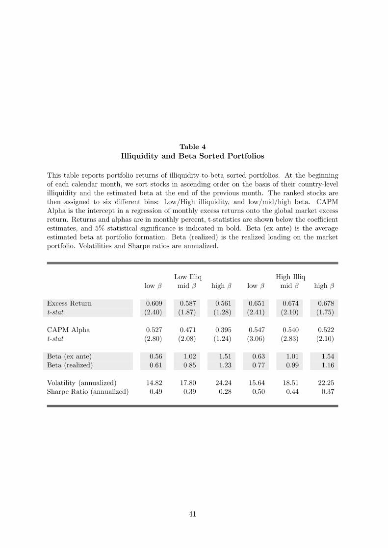
Table 4

Illiquidity and Beta Sorted Portfolios

This table reports portfolio returns of illiquidity-to-beta sorted portfolios. At the beginningof each calendar month, we sort stocks in ascending order on the basis of their country-levelilliquidity and the estimated beta at the end of the previous month. The ranked stocks arethen assigned to six different bins: Low/High illiquidity, and low/mid/high beta. CAPMAlpha is the intercept in a regression of monthly excess returns onto the global market excessreturn. Returns and alphas are in monthly percent, t-statistics are shown below the coefficientestimates, and 5% statistical significance is indicated in bold. Beta (ex ante) is the averageestimated beta at portfolio formation. Beta (realized) is the realized loading on the marketportfolio. Volatilities and Sharpe ratios are annualized.

Low Illiq High Illiqlow β mid β high β low β mid β high β

Excess Return 0.609 0.587 0.561 0.651 0.674 0.678t-stat (2.40) (1.87) (1.28) (2.41) (2.10) (1.75)

CAPM Alpha 0.527 0.471 0.395 0.547 0.540 0.522t-stat (2.80) (2.08) (1.24) (3.06) (2.83) (2.10)

Beta (ex ante) 0.56 1.02 1.51 0.63 1.01 1.54Beta (realized) 0.61 0.85 1.23 0.77 0.99 1.16

Volatility (annualized) 14.82 17.80 24.24 15.64 18.51 22.25Sharpe Ratio (annualized) 0.49 0.39 0.28 0.50 0.44 0.37

41

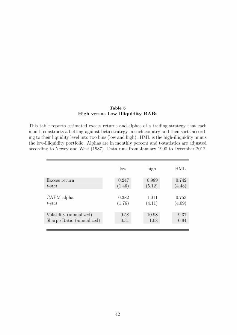
Table 5

High versus Low Illiquidity BABs

This table reports estimated excess returns and alphas of a trading strategy that eachmonth constructs a betting-against-beta strategy in each country and then sorts accord-ing to their liquidity level into two bins (low and high). HML is the high-illiquidity minusthe low-illiquidity portfolio. Alphas are in monthly percent and t-statistics are adjustedaccording to Newey and West (1987). Data runs from January 1990 to December 2012.

low high HML

Excess return 0.247 0.989 0.742t-stat (1.46) (5.12) (4.48)

CAPM alpha 0.382 1.011 0.753t-stat (1.76) (4.11) (4.09)

Volatility (annualized) 9.58 10.98 9.37Sharpe Ratio (annualized) 0.31 1.08 0.94

42

Table 6

BAIL versus BAB

This table reports estimated excess returns and alphas for the BAIL and BAB tradingstrategies. BAIL is a self-financing portfolio that is long the high illiquidity to betastocks and short the low illiquidity to beta stocks. BAB is long the low-beta portfolioand short the high-beta portfolio. The alphas are calculated from regressions of monthlyexcess returns onto the market (CAPM). Alphas are in monthly percent and t-statisticsare adjusted according to Newey and West (1987). Data runs from January 1990 toDecember 2012.

BAB BAIL

Excess Returns 0.741 0.827t-stat (3.51) (3.53)

CAPM alpha 0.731 0.791t-stat (2.48) (3.53)

Volatility (annualized) 12.10 13.51Sharpe Ratio (annualized) 0.73 0.73

43

Table 7

Illiquidity and Beta Sorted Portfolios Orthogonalized

This table reports portfolio returns of illiquidity-to-beta sorted portfolios where illiquidity mea-sures have been orthogonalized with respect to the Amihud (2002) market illiquidity measure.At the beginning of each calendar month, we sort stocks in ascending order on the basis oftheir country-level illiquidity and the estimated beta at the end of the previous month. Theranked stocks are then assigned to six different bins: Low/High illiquidity, and low/mid/highbeta. CAPM Alpha is the intercept in a regression of monthly excess returns onto the globalmarket excess return. Returns and alphas are in monthly percent, t-statistics are shown belowthe coefficient estimates, and 5% statistical significance is indicated in bold. Beta (ex ante) isthe average estimated beta at portfolio formation. Beta (realized) is the realized loading onthe market portfolio. Volatilities and Sharpe ratios are annualized. Using these orthogonalizedilliquidity measures, we build a BAIL strategy that is long the high illiquidity to beta stocksand short the low illiquidity to beta stocks.

Low Illiq High Illiqlow β mid β high β low β mid β high β BAIL

Excess Return 0.521 0.745 0.794 0.887 0.963 1.056 0.783t-stat (1.53) (1.69) (1.27) (3.26) (2.51) (1.85) (2.21)

CAPM Alpha 0.772 0.731 0.510 1.033 0.951 0.874 0.783t-stat (2.29) (2.36) (1.80) (3.52) (4.32) (5.06) (2.22)

Beta (ex-ante) 0.53 0.87 1.41 0.56 0.88 1.39 0.00Beta (realized) 0.51 0.85 1.44 0.57 0.86 1.33 0.14

Volatility (annualized) 15.32 19.61 28.05 12.13 17.26 25.52 15.81Sharpe Ratio (annualized) 0.41 0.45 0.34 0.87 0.67 0.50 0.59

44

Appendix C Figures

1995 2000 2005 2010

in b

p

0

5

10

United States

1995 2000 2005 2010

in b

p

0

5

10

15Germany

1995 2000 2005 2010

in b

p

0

10

20

United Kingdom

1995 2000 2005 2010

in b

p

0

10

20Canada

1995 2000 2005 2010

in b

p

0

5

10

Japan

1995 2000 2005 2010

in b

p

0

20

40Switzerland

Figure 1. Illiquidity Measures All Countries

This figure plots country-level illiquidity proxies for six different countries: United States,Germany, United Kingdom, Canada, Japan, and Switzerland. Illiquidity is calculatedas the average squared deviation of observed bond prices from those implied by a fittedyield curve using the method of Svensson (1994). Measures are in basis points. Data ismonthly and runs from January 1990 to December 2012.

45

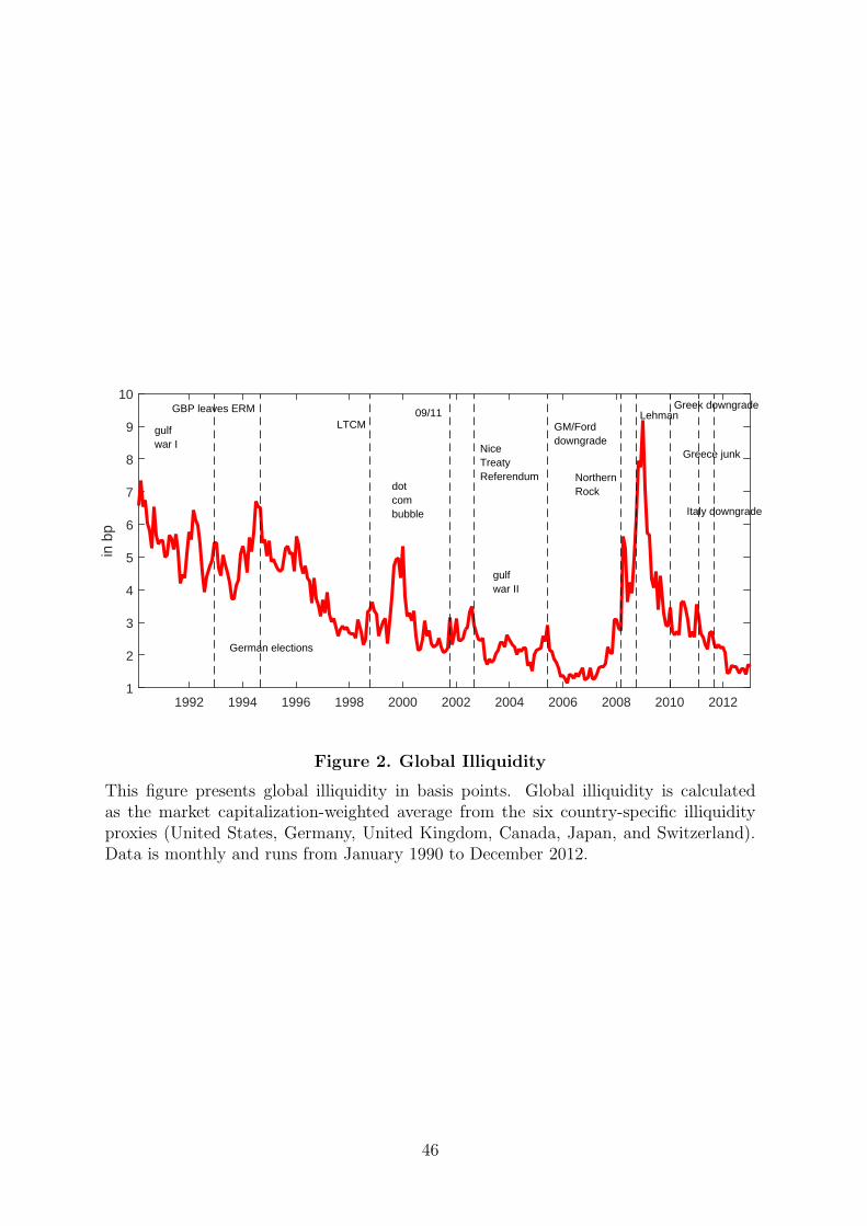
1992 1994 1996 1998 2000 2002 2004 2006 2008 2010 2012

in b

p

1

2

3

4

5

6

7

8

9

10GBP leaves ERM

German elections

LTCM09/11

NiceTreatyReferendum

GM/Forddowngrade

NorthernRock

LehmanGreek downgrade

Greece junk

Italy downgrade

gulfwar II

gulfwar I

dotcombubble

Figure 2. Global Illiquidity

This figure presents global illiquidity in basis points. Global illiquidity is calculatedas the market capitalization-weighted average from the six country-specific illiquidityproxies (United States, Germany, United Kingdom, Canada, Japan, and Switzerland).Data is monthly and runs from January 1990 to December 2012.

46

1990 1995 2000 2005 2010−0.1

0

0.1

0.2

0.3

0.4

0.5

0.6

0.7ERMcrisis

Asiancrisis dot com

bubble

Lehman

Eurocrisis

Figure 3. Average Conditional Correlation of Country-Specific IlliquidityMeasures

This figure present the conditional average correlation among all six country-specific illiq-uidity proxies (United States, Germany, United Kingdom, Canada, Japan, and Switzer-land). Conditional correlations are calculated using a rolling window of three years usingdaily data. Data is sampled monthly and runs from January 1990 to December 2012.

47

1990 1992 1994 1996 1998 2000 2002 2004 2006 2008 2010 20120

1

2

3

4

5

6

7

Figure 4. Cross-Sectional Standard Deviation of Country-Specific IlliquidityMeasures

This figure present the cross-sectional standard deviation of country-specific illiquiditymeasures (United States, Germany, United Kingdom, Canada, Japan, and Switzerland).The standard deviations are calculated monthly, the data runs from January 1990 toDecember 2012.

48

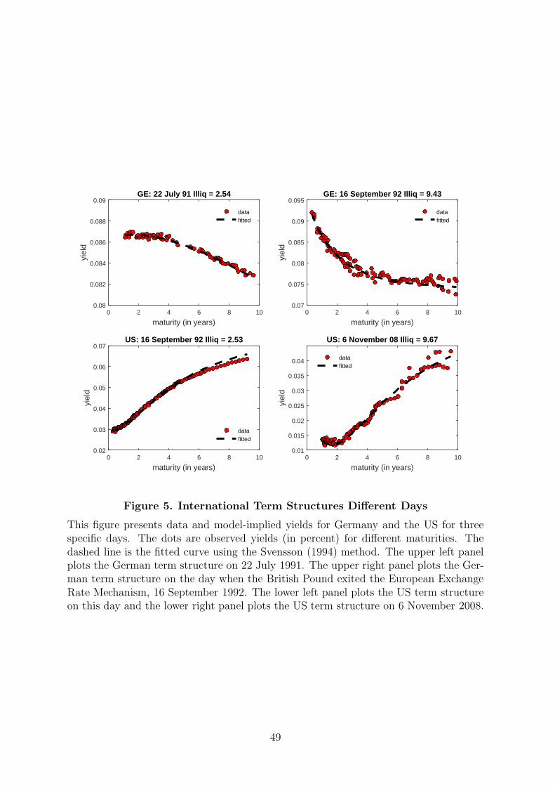
maturity (in years)0 2 4 6 8 10

yiel

d

0.08

0.082

0.084

0.086

0.088

0.09GE: 22 July 91 Illiq = 2.54

datafitted


yiel

d

0.07

0.075

0.08

0.085

0.09

0.095GE: 16 September 92 Illiq = 9.43

datafitted


yiel

d

0.02

0.03

0.04

0.05

0.06

0.07US: 16 September 92 Illiq = 2.53

datafitted


yiel

d

0.01

0.015

0.02

0.025

0.03

0.035

0.04

US: 6 November 08 Illiq = 9.67

datafitted

Figure 5. International Term Structures Different Days

This figure presents data and model-implied yields for Germany and the US for threespecific days. The dots are observed yields (in percent) for different maturities. Thedashed line is the fitted curve using the Svensson (1994) method. The upper left panelplots the German term structure on 22 July 1991. The upper right panel plots the Ger-man term structure on the day when the British Pound exited the European ExchangeRate Mechanism, 16 September 1992. The lower left panel plots the US term structureon this day and the lower right panel plots the US term structure on 6 November 2008.

49

low 2 3 4 high−0.1

0

0.1

0.2

0.3

0.4

0.5

0.6

inte

rcep

t / s

lope

SM

L (in

%)

interceptslope

Figure 6. Intercept and Slope Security Market Line

This figure plots the average intercept and slope of the security market line for differentglobal illiquidity quintiles. The full sample period is from January 1990 to December2012.

50

2004 2006 2008 2010 20120

2

4

6

8

10

12

cum

ulat

ive

retu

rn

bailbab

Figure 7. BAIL versus BAB cumulative returns

This figure plots the cumulative return of BAIL and BAB. Data is monthly and startsin 2003 and ends in 2012.

51

InternationalIlliquidity - phd-finance.uzh.ch4a2b68eb-da0f-4bf3... · In this paper, we study the...

Documents

Transcript of InternationalIlliquidity - phd-finance.uzh.ch4a2b68eb-da0f-4bf3... · In this paper, we study the...