International TradeInternational Trade International TradeInternational Trade

Chapter 1

Introduction to International Trade

1.1 The definition of international trade

International trade can be defined as the exchange of goods and services produced in one country (or district) with those produced in another country(or district).

The reasons for international tradeThe reasons for international trade

A. The uneven distribution of natural resources

B. International specialization

C. Different Patterns of demand among nations

D.  Economies of scale

E. Innovation or variety of style

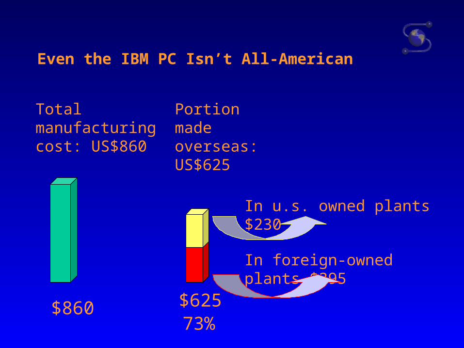
$860 $62573%

Even the IBM PC Isn’t All-American

Total manufacturing cost: US$860

Portion made overseas: US$625

In u.s. owned plants $230

In foreign-owned plants $395

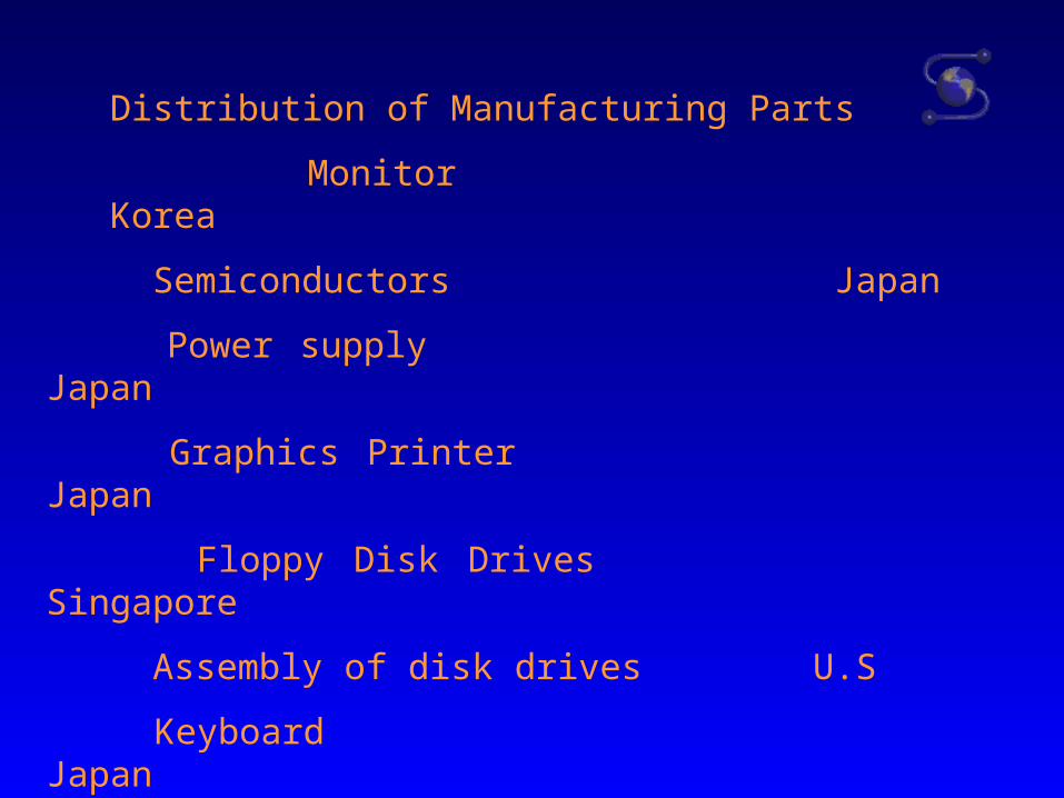
Distribution of Manufacturing Parts

Monitor Korea

Semiconductors Japan

Power supply Japan

Graphics Printer Japan

Floppy Disk Drives Singapore

Assembly of disk drives U.S

Keyboard Japan

Case and final Assembly U.S

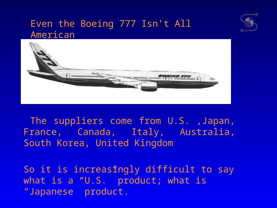
The suppliers come from U.S. ,Japan, France, Canada, Italy, Australia, South Korea, United Kingdom

Even the Boeing 777 Isn’t All American

So it is increasingly difficult to say what is a “U.S.” product; what is “Japanese” product.

1.2. The history of international trade development

The first beginning of international trade

The development of international trade in different social period

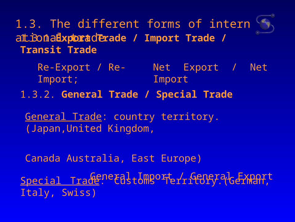
1.3.1.Export Trade / Import Trade / Transit Trade

1.3. The different forms of international trade

Re-Export / Re-Import; Net Export / Net Import

1.3.2. General Trade / Special Trade

General Trade: country territory. (Japan,United Kingdom,

Canada Australia, East Europe)

General Import / General ExportSpecial Trade: Customs Territory.(German, Italy, Swiss)

1.3.3. Visible Trade / Invisible Trade

1.3.4 Direct Trade / Indirect Trade / Entrepot Trade

1.3.5 Trade by Roadway / Trade by Seaway /

Trade by Airway / Trade by Mail Order

1.3.6  Free-Liquidation Trade / Barter Trade

1.4 . Another basic concepts about international trade

1.4.1.  amount of foreign trade

total amount of import and export for a country in definite period.

1.4.2. amount of international trade

total amount of export for all countries in definite period.

    1.4.3. trade balance

favorable balance: export >import (surplus)

adverse balance: export<import (deficit)

1.4.4.   commodity structure

primary commodities

Industry commodities (finished goods)

1.4.5. factors of production

a. capital,

b. human resources or labor

c. property resources including land

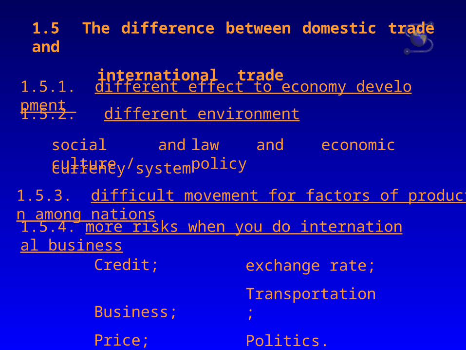
1.5 The difference between domestic trade and

international trade

1.5.1.  different effect to economy development

1.5.2.  different environment

social and culture / law and economic policy

currency system

1.5.3.  difficult movement for factors of production among nations

1.5.4. more risks when you do international business

Credit;

Business;

Price;

exchange rate;

Transportation;

Politics.

1.6 国际商务环境1.6 国际商务环境

进口商进口商 生产厂家生产厂家

海关海关

银行银行商检局商检局

外运公司外运公司 保险公司保险公司

税务局税务局

出口商出口商

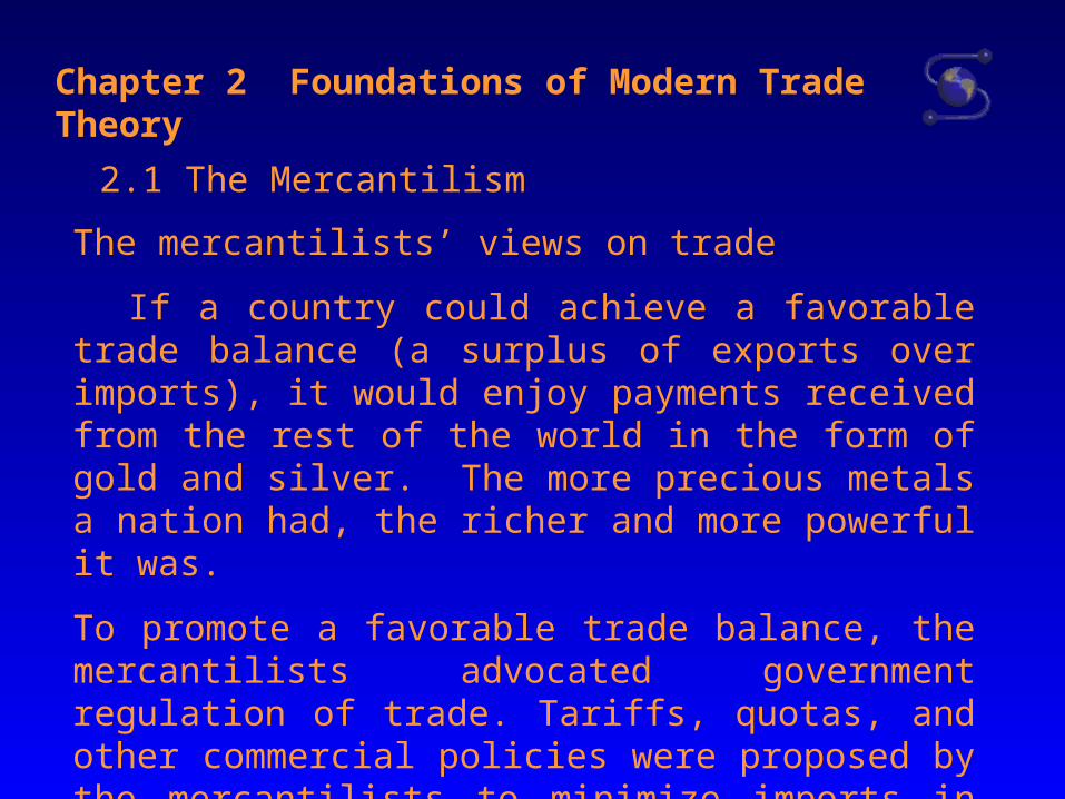
Chapter 2 Foundations of Modern Trade Theory

2.1 The Mercantilism

The mercantilists’ views on trade

If a country could achieve a favorable trade balance (a surplus of exports over imports), it would enjoy payments received from the rest of the world in the form of gold and silver. The more precious metals a nation had, the richer and more powerful it was.

To promote a favorable trade balance, the mercantilists advocated government regulation of trade. Tariffs, quotas, and other commercial policies were proposed by the mercantilists to minimize imports in order to protect a nation’s trade position.

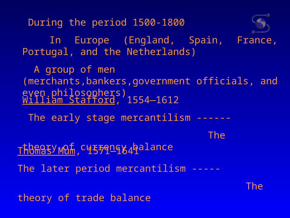
William Stafford, 1554—1612

The early stage mercantilism ------

The theory of currency balance

Thomas Mum, 1571—1641

The later period mercantilism -----

The theory of trade balance

During the period 1500-1800

In Europe (England, Spain, France, Portugal, and the Netherlands)

A group of men (merchants,bankers,government officials, and even philosophers)

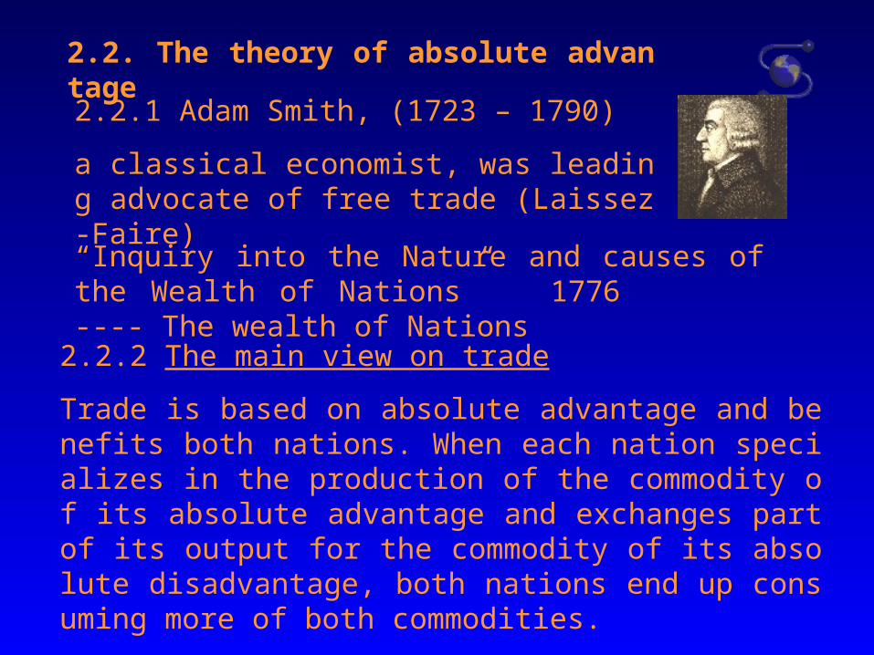
2.2. The theory of absolute advantage

2.2.1 Adam Smith, (1723 – 1790)

a classical economist, was leading advocate of free trade (Laissez-Faire)

“Inquiry into the Nature and causes of the Wealth of Nations” 1776 ---- The wealth of Nations

2.2.2 The main view on trade

Trade is based on absolute advantage and benefits both nations. When each nation specializes in the production of the commodity of its absolute advantage and exchanges part of its output for the commodity of its absolute disadvantage, both nations end up consuming more of both commodities.

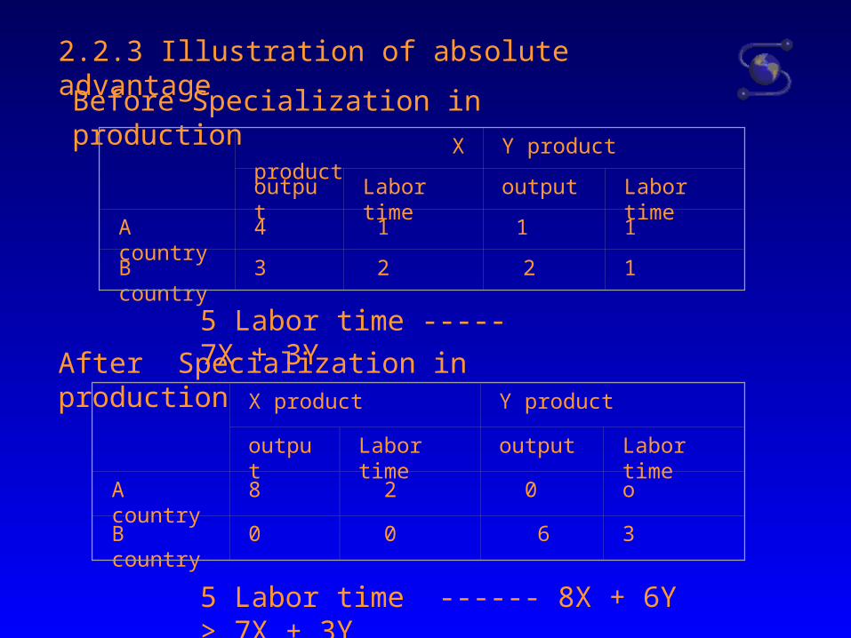
2.2.3 Illustration of absolute advantage

Before Specialization in production  

X product Y product

output Labor time output Labor time

A country 4 1 1 1

B country 3 2 2 1

5 Labor time ----- 7X + 3Y

After Specialization in production    X product Y product

output Labor time output Labor time

A country 8 2 0 o

B country 0 0 6 3

5 Labor time ------ 8X + 6Y > 7X + 3Y

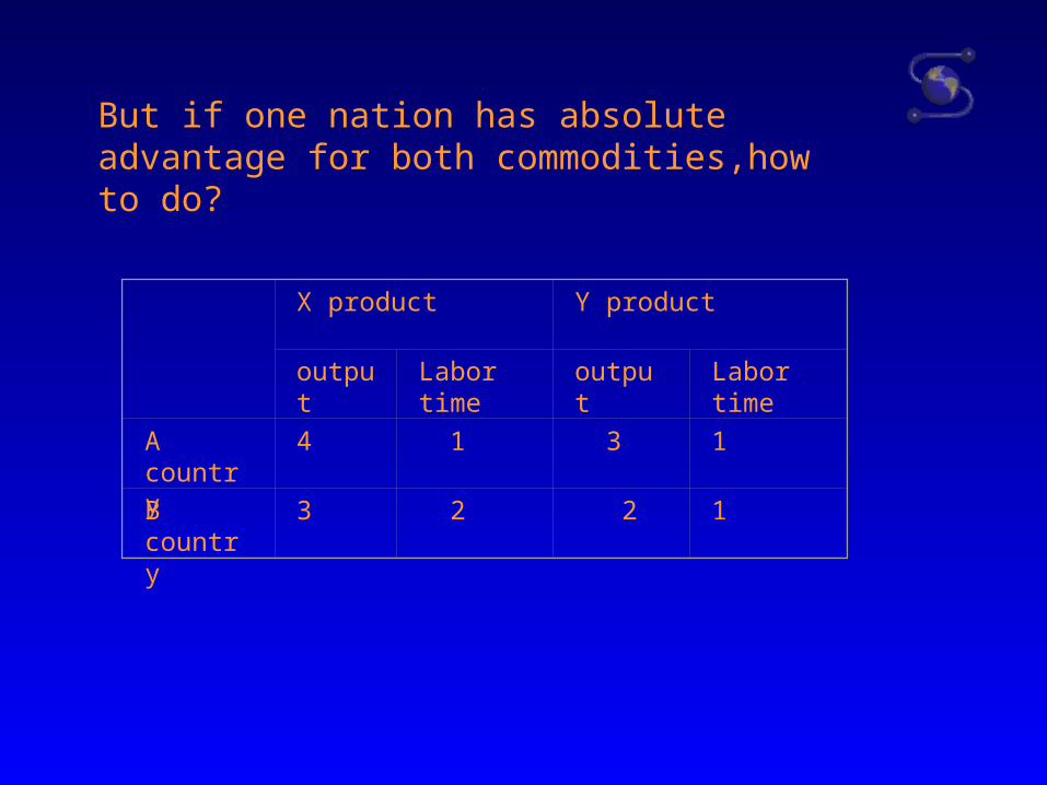
But if one nation has absolute advantage for both commodities,how to do?

 

X product Y product

output Labor time

output Labor time

A country

4 1 3 1

B country

3 2 2 1

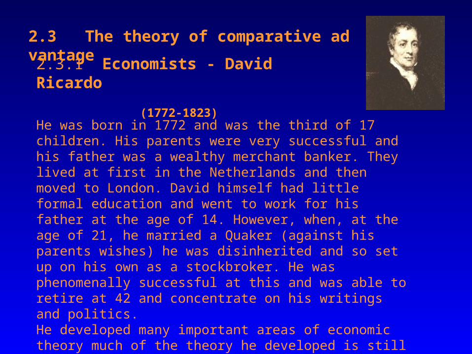
2.3 The theory of comparative advantage

2.3.1 Economists - David Ricardo

(1772-1823)                                

He was born in 1772 and was the third of 17 children. His parents were very successful and his father was a wealthy merchant banker. They lived at first in the Netherlands and then moved to London. David himself had little formal education and went to work for his father at the age of 14. However, when, at the age of 21, he married a Quaker (against his parents wishes) he was disinherited and so set up on his own as a stockbroker. He was phenomenally successful at this and was able to retire at 42 and concentrate on his writings and politics. He developed many important areas of economic theory much of the theory he developed is still used and taught today.

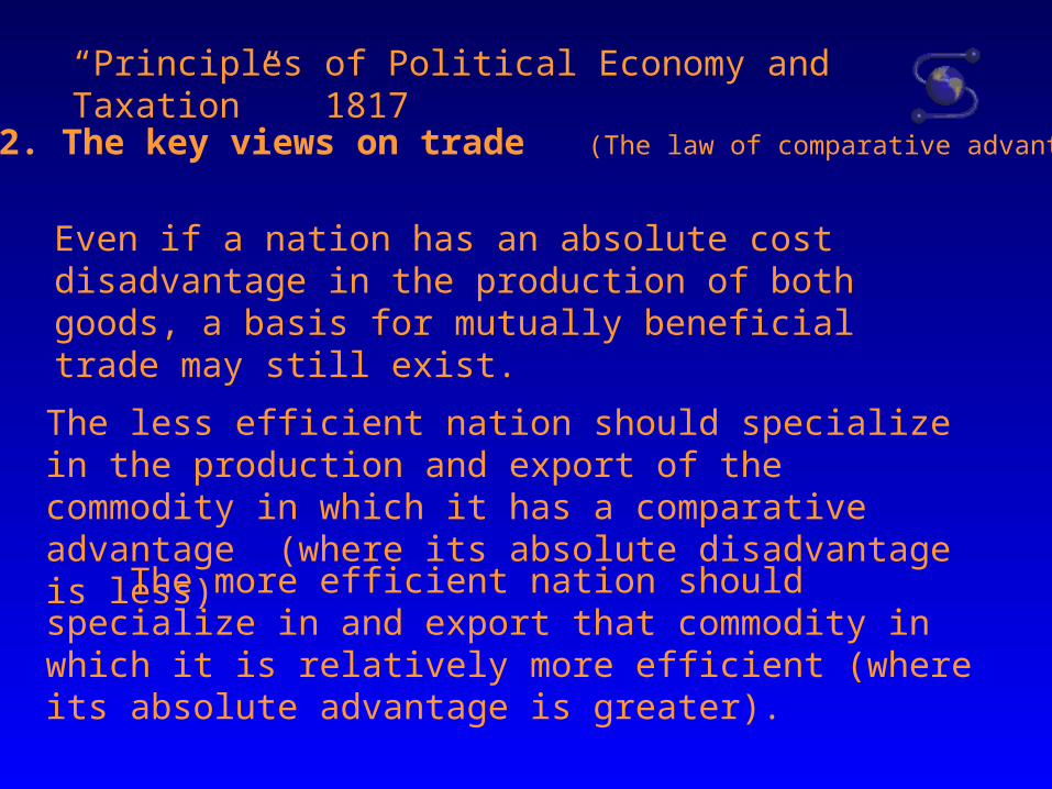
Even if a nation has an absolute cost disadvantage in the production of both goods, a basis for mutually beneficial trade may still exist.

2.3.2. The key views on trade (The law of comparative advantage)

The less efficient nation should specialize in the production and export of the commodity in which it has a comparative advantage (where its absolute disadvantage is less)

The more efficient nation should specialize in and export that commodity in which it is relatively more efficient (where its absolute advantage is greater).

“Principles of Political Economy and Taxation” 1817

 

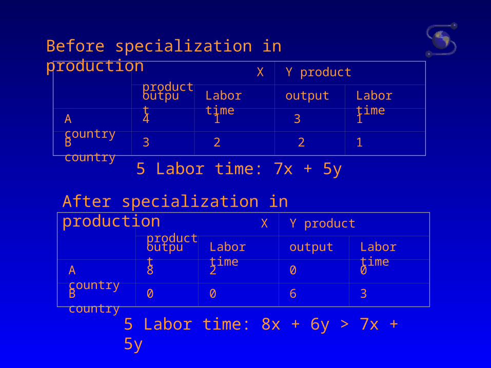
X product Y product

output Labor time output Labor time

A country 4 1 3 1

B country 3 2 2 1

Before specialization in production

5 Labor time: 7x + 5y

After specialization in production  

X product Y product

output Labor time output Labor time

A country 8 2 0 0

B country 0 0 6 3

5 Labor time: 8x + 6y > 7x + 5y

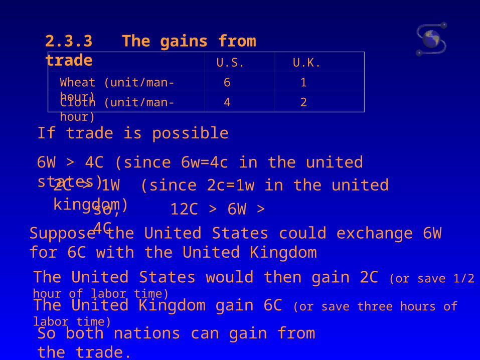
2.3.3 The gains from trade   U.S. U.K.

Wheat (unit/man-hour) 6 1

Cloth (unit/man-hour) 4 2

If trade is possible

6W > 4C (since 6w=4c in the united states)

2C > 1W (since 2c=1w in the united kingdom)

so, 12C > 6W > 4C

Suppose the United States could exchange 6W for 6C with the United Kingdom

The United States would then gain 2C (or save 1/2 hour of labor time)

The United Kingdom gain 6C (or save three hours of labor time)

So both nations can gain from the trade.

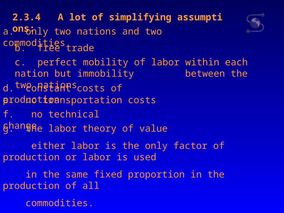
2.3.4 A lot of simplifying assumptions:

a. only two nations and two commodities

b. free trade

c. perfect mobility of labor within each nation but immobility between the two nations

d. constant costs of productione. no transportation costs

f. no technical change

g. the labor theory of value

either labor is the only factor of production or labor is used

in the same fixed proportion in the production of all

commodities.

labor is homogeneous

2.4. The opportunity cost theory

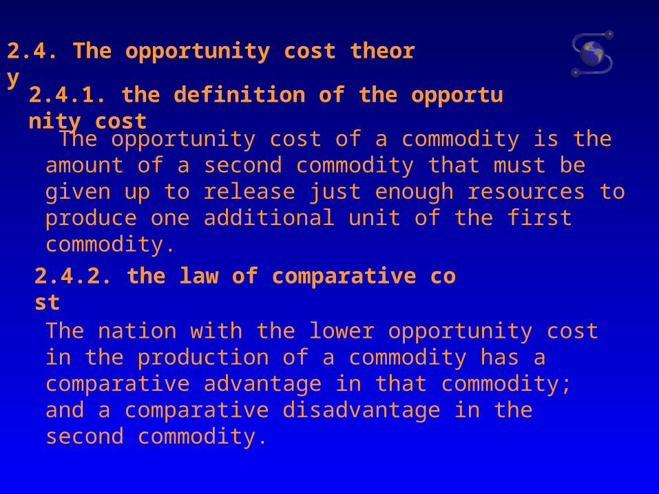
2.4.1. the definition of the opportunity cost

The opportunity cost of a commodity is the amount of a second commodity that must be given up to release just enough resources to produce one additional unit of the first commodity.

2.4.2. the law of comparative cost

The nation with the lower opportunity cost in the production of a commodity has a comparative advantage in that commodity; and a comparative disadvantage in the second commodity.

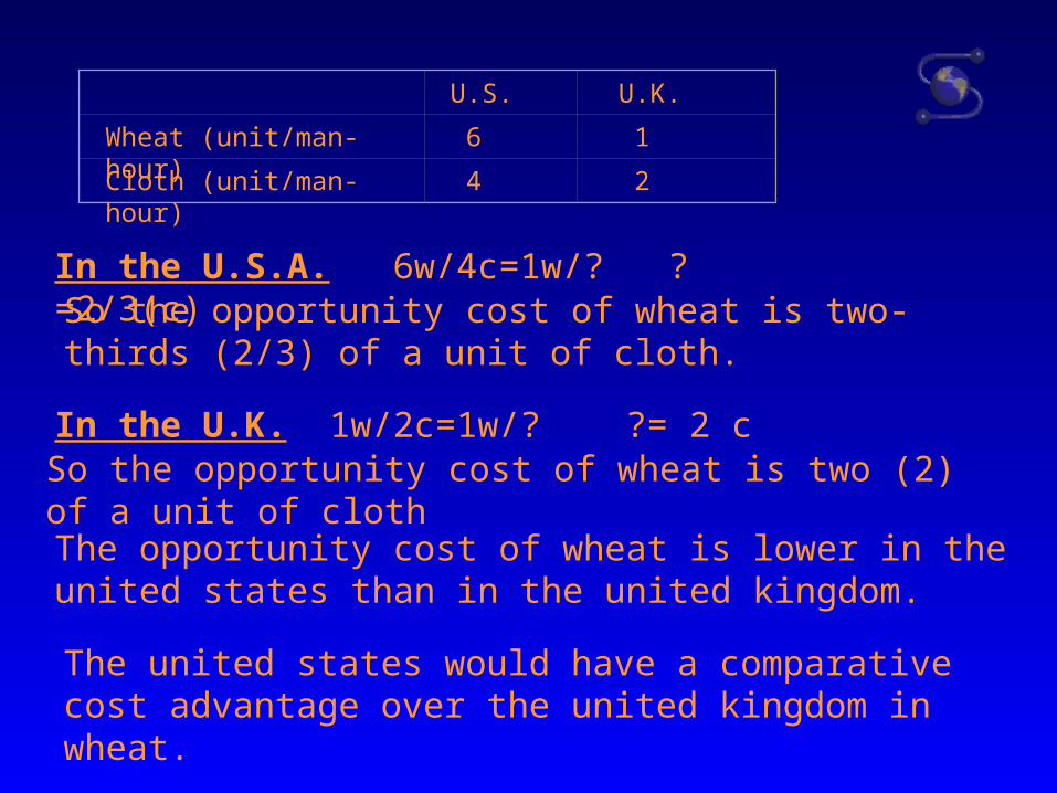
  U.S. U.K.

Wheat (unit/man-hour) 6 1

Cloth (unit/man-hour) 4 2

In the U.S.A. 6w/4c=1w/? ?=2/3(c)So the opportunity cost of wheat is two-thirds (2/3) of a unit of cloth.

In the U.K. 1w/2c=1w/? ?= 2 cSo the opportunity cost of wheat is two (2) of a unit of cloth

The opportunity cost of wheat is lower in the united states than in the united kingdom.

The united states would have a comparative cost advantage over the united kingdom in wheat.

2.4.3. Transformation schedules

production possibility curve;

production possibility frontier

This schedule shows various alternative combinations of two goods that a nation can produce when all of its factor inputs (land, labor, capital, entrepreneurship) are used in their most efficient manner.

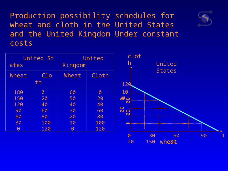
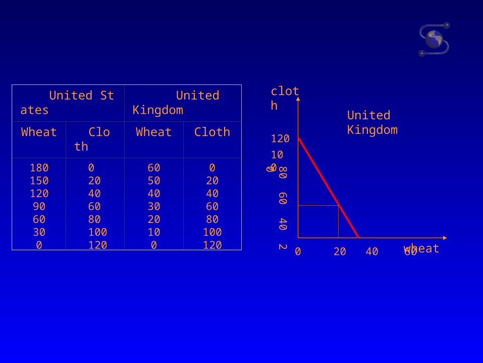
United States United Kingdom

Wheat Cloth Wheat Cloth

1801501209060300

020406080100120

6050403020100

020406080100120

Production possibility schedules for wheat and cloth in the United States and the United Kingdom Under constant costs

120

wheat

clothUnited States

0 30 60 90 120 150 180

100

80 60 40 20

United States United Kingdo

m

Wheat Cloth Wheat Cloth

1801501209060300

020406080100120

6050403020100

020406080100120

120

100

80 60 40 20

0 20 40 60 wheat

cloth

United Kingdom

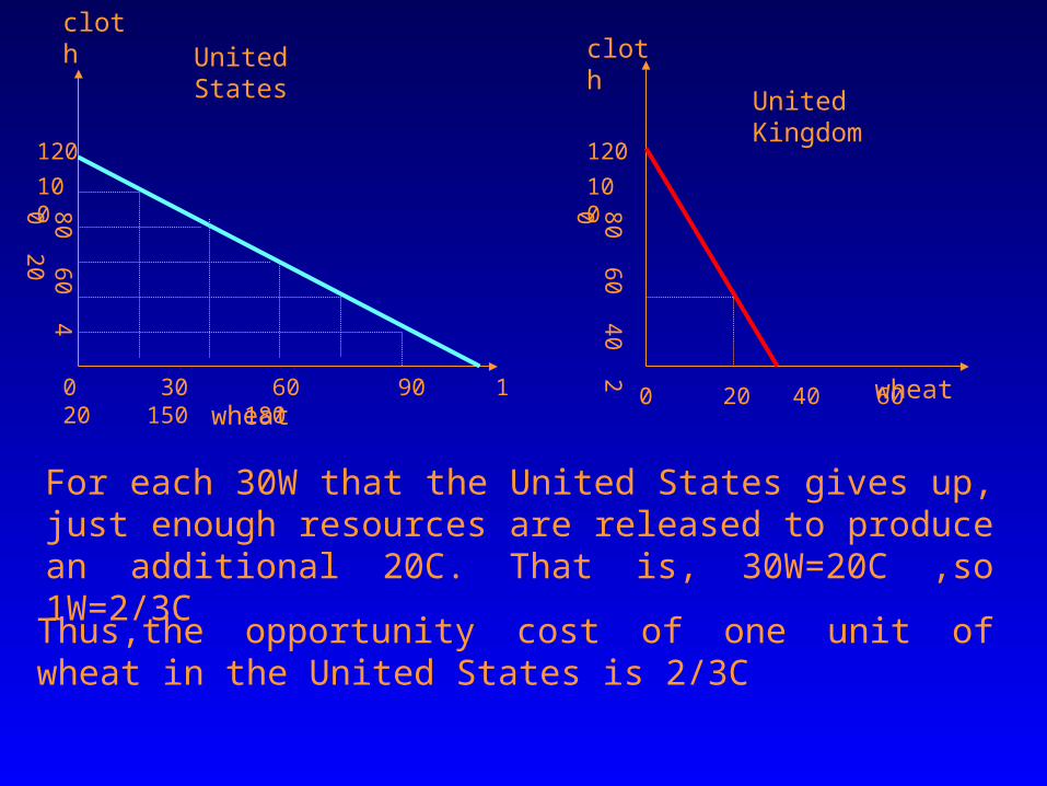
For each 30W that the United States gives up, just enough resources are released to produce an additional 20C. That is, 30W=20C ,so 1W=2/3C

Thus,the opportunity cost of one unit of wheat in the United States is 2/3C

120

wheat

clothUnited States

0 30 60 90 120 150 180

100

80 60 40 20

120

100

80 60 40 20

0 20 40 60 wheat

cloth

United Kingdom

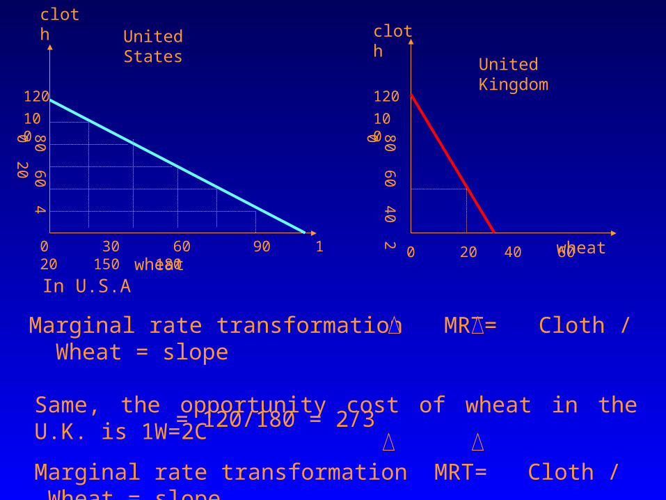
In U.S.A

Marginal rate transformation MRT= Cloth / Wheat = slope

= 120/180 = 2/3Same, the opportunity cost of wheat in the U.K. is 1W=2C

Marginal rate transformation MRT= Cloth / Wheat = slope

= 120 / 60 = 2

120

wheat

clothUnited States

0 30 60 90 120 150 180

100

80 60 40 20

120

100

80 60 40 20

0 20 40 60 wheat

cloth

United Kingdom

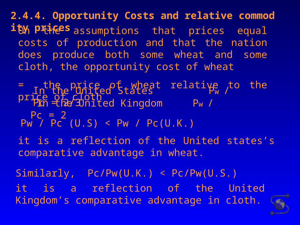
2.4.4. Opportunity Costs and relative commodity prices

On the assumptions that prices equal costs of production and that the nation does produce both some wheat and some cloth, the opportunity cost of wheat

= the price of wheat relative to the price of cloth

In the United States Pw / Pc = 2/3 In the United Kingdom Pw / Pc = 2

Pw / Pc (U.S) < Pw / Pc(U.K.)

it is a reflection of the United states’s comparative advantage in wheat.

Similarly, Pc/Pw(U.K.) < Pc/Pw(U.S.)

it is a reflection of the United Kingdom’s comparative advantage in cloth.

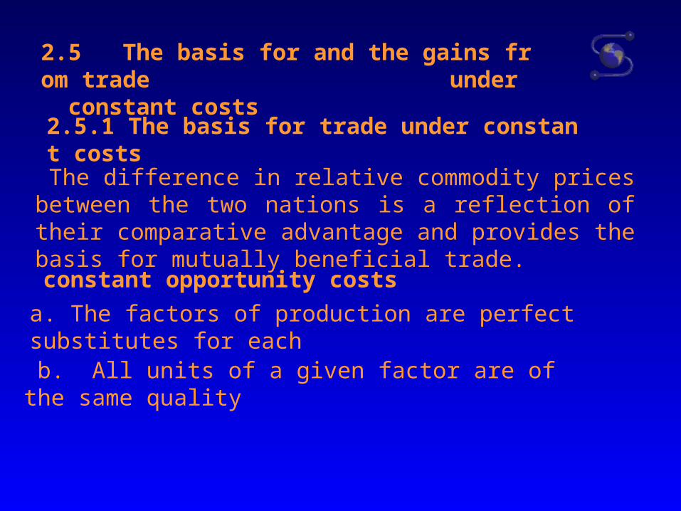
The difference in relative commodity prices between the two nations is a reflection of their comparative advantage and provides the basis for mutually beneficial trade.

2.5 The basis for and the gains from trade under constant costs

constant opportunity costs

a. The factors of production are perfect substitutes for each

b. All units of a given factor are of the same quality

2.5.1 The basis for trade under constant costs

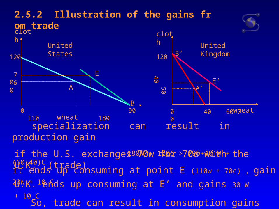
2.5.2 Illustration of the gains from trade

120

wheat

cloth

United States

0 90 110 180

70 60

E

B

A

120

50 40

0 40 60 70 wheat

cloth

United KingdomB’

E’A’

specialization can result in production gain

180W + 120C > (90+40)W + (60+40)C

if the U.S. exchanges 70w for 70c with the U.K, (trade)

it ends up consuming at point E (110w + 70c) , gain 20W + 10 C

U.K. ends up consuming at E’ and gains 30 W + 10 C

So, trade can result in consumption gains for both countries.

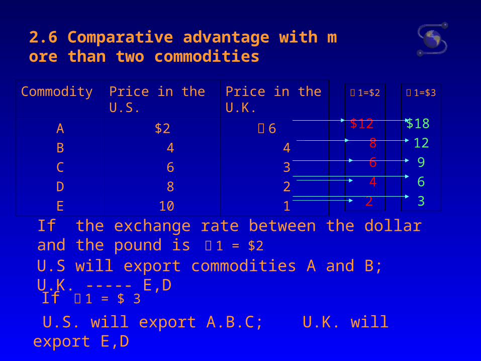
2.6 Comparative advantage with more than two commodities

Commodity Price in the U.S. Price in the U.K.

A

B

C

D

E

$2

4

6

8

10

￡ 6

4

3

2

1

If the exchange rate between the dollar and the pound is ￡ 1 = $2

U.S will export commodities A and B; U.K. ----- E,D

If ￡ 1 = $ 3

U.S. will export A.B.C; U.K. will export E,D

￡ 1=$2

$12

8

6

4

2

￡ 1=$3

$18

12

9

6

3

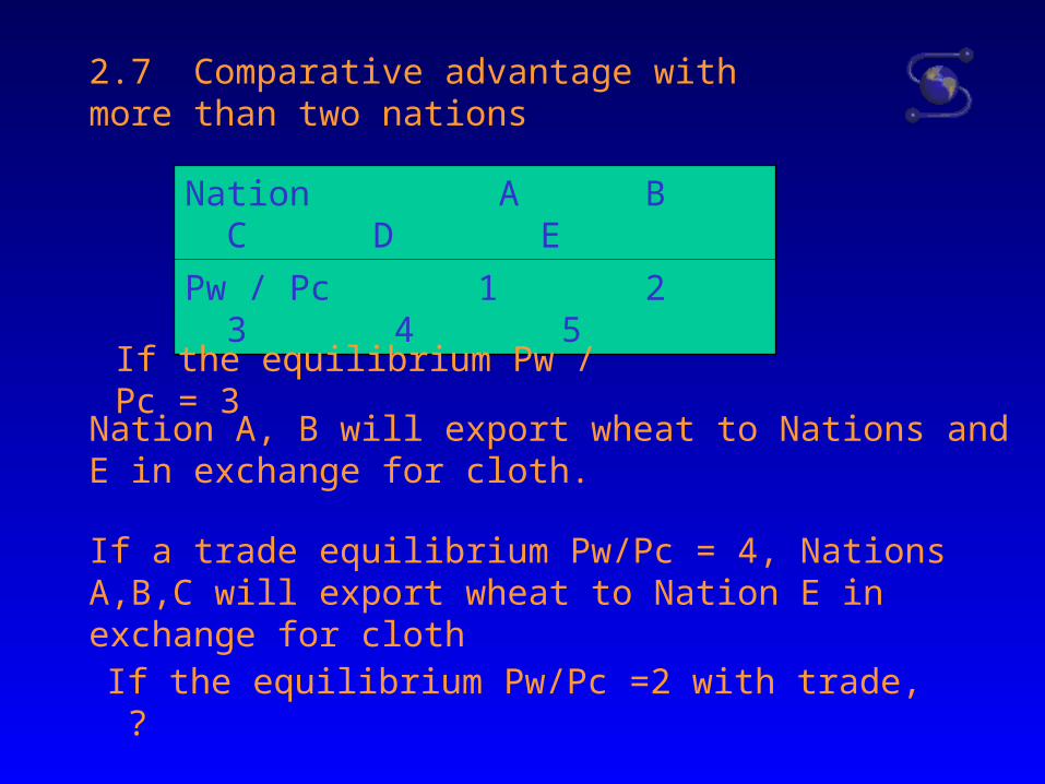
2.7 Comparative advantage with more than two nations

Nation A B C D E

Pw / Pc 1 2 3 4 5

If the equilibrium Pw / Pc = 3

Nation A, B will export wheat to Nations and E in exchange for cloth.

If a trade equilibrium Pw/Pc = 4, Nations A,B,C will export wheat to Nation E in exchange for cloth

If the equilibrium Pw/Pc =2 with trade, ?

Chapter 3 The Standard Theory of International Trade

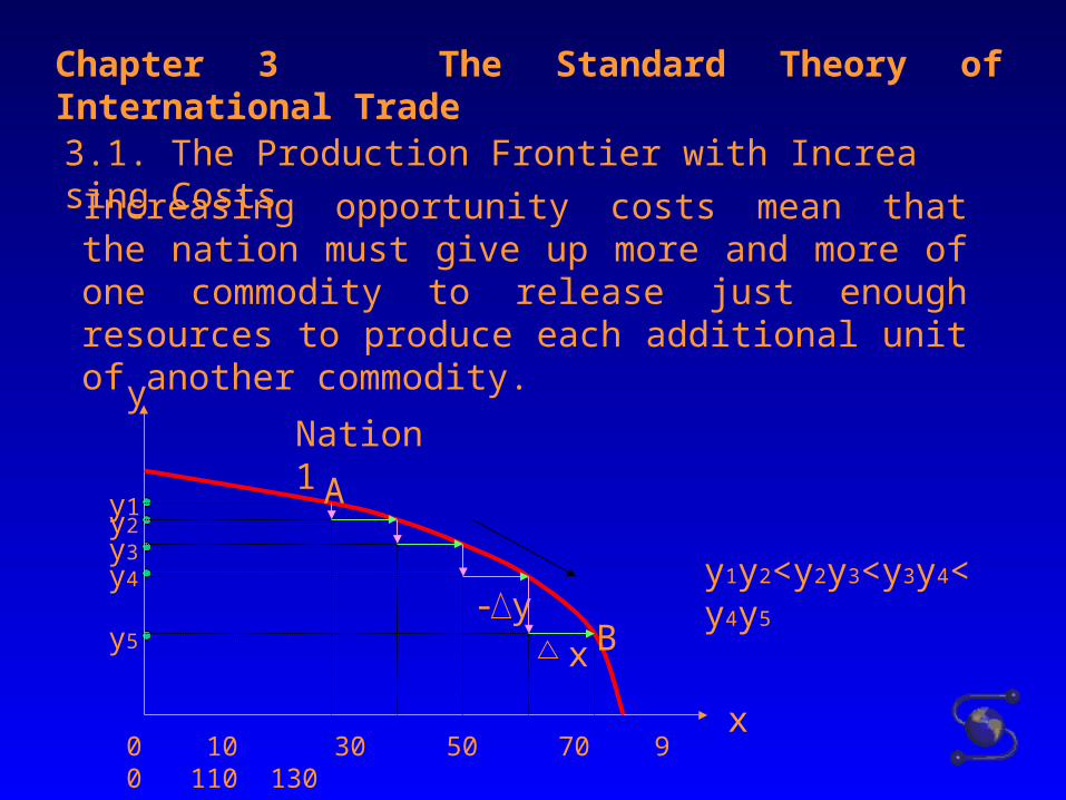
3.1. The Production Frontier with Increasing Costs

Increasing opportunity costs mean that the nation must give up more and more of one commodity to release just enough resources to produce each additional unit of another commodity.

0 10 30 50 70 90 110 130

Nation 1y

x

y-x

A

B

y3

y1y2

y4

y5

y1y2<y2y3<y3y4< y4y5

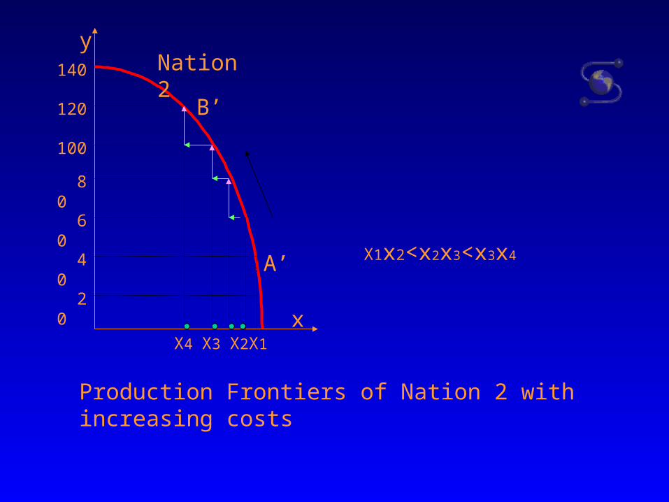
140

120

100

80

60

40

20

y

x

A’

B’

Nation 2

X4 X3 X2X1

X1x2<x2x3<x3x4

Production Frontiers of Nation 2 with increasing costs

3.1.2 Reasons for increasing opportunity costs and

different Production frontiers

a. Resources or factors of production are not homogeneous

b. Resources or factors of production are not used in the

same fixed proportion or intensity in the production of

all commodities.

The difference in the production frontiers of two nations is due to the fact that the two nations have different factor endowments or resources at their disposal and /or use different technologies in production.

c.

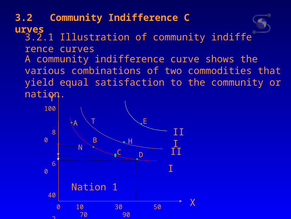
3.2 Community Indifference Curves

3.2.1 Illustration of community indifference curves

A community indifference curve shows the various combinations of two commodities that yield equal satisfaction to the community or nation.

N

Nation 1

0 10 30 50 70 90

100

80

60

40

20

H

ET

C

I

II

III

Y

X

A

B

D

3.2.2 The marginal Rate of Substitution (MRS)

MRS of X for Y in consumption refers to the amount of Y that a nation could give up for one extra unit of X and still remain on the same indifference curve.

In Nation 1 ,the substitution of x for y ,MRS(N) > MRS(A)

The decline in MRS or absolute slope of an indifference curve is a reflection or the fact that the more of X and the less of Y a nation consumes;

The declining slope of the curve reflects the diminishing marginal rate of substitution (MRS) of X for Y in consumption.

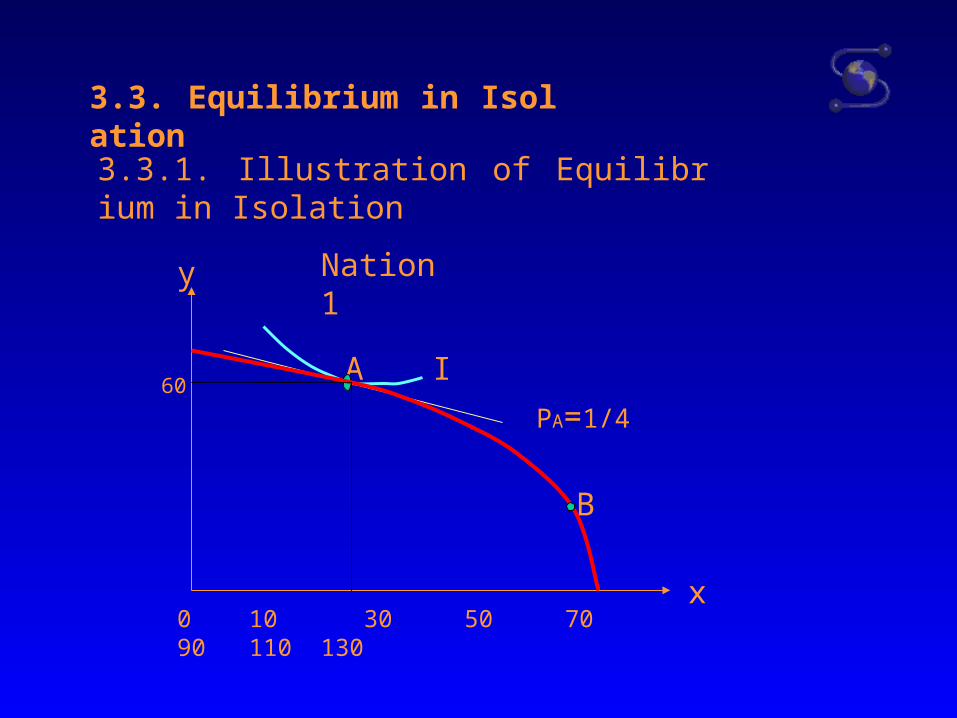
3.3. Equilibrium in Isolation

3.3.1. Illustration of Equilibrium in Isolation

PA=1/4

y

x

A

0 10 30 50 70 90 110 130

Nation 1

B

I60

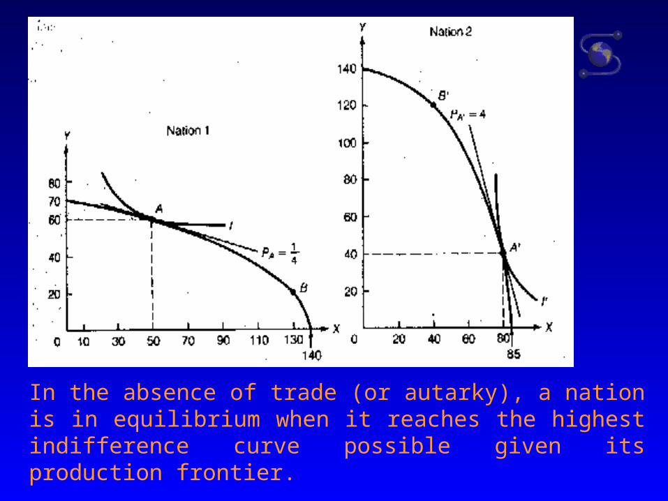
In the absence of trade (or autarky), a nation is in equilibrium when it reaches the highest indifference curve possible given its production frontier.

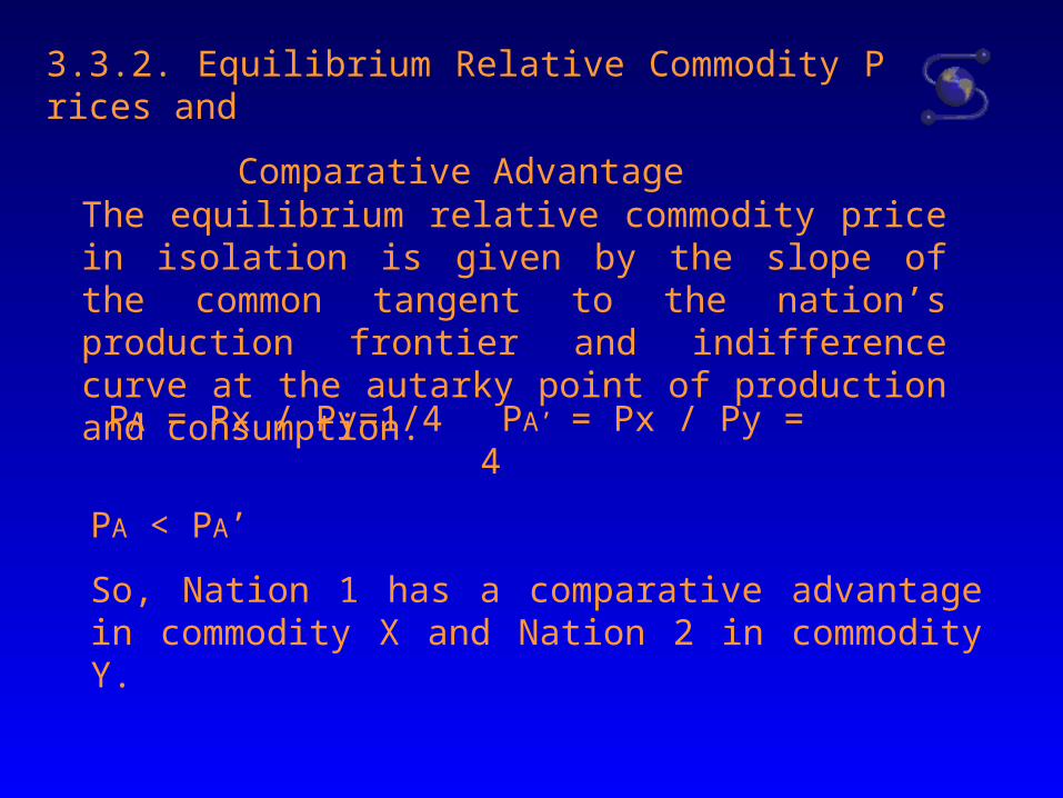
3.3.2. Equilibrium Relative Commodity Prices and

Comparative Advantage

The equilibrium relative commodity price in isolation is given by the slope of the common tangent to the nation’s production frontier and indifference curve at the autarky point of production and consumption.

PA = Px / Py=1/4 PA’ = Px / Py = 4

PA < PA’

So, Nation 1 has a comparative advantage in commodity X and Nation 2 in commodity Y.

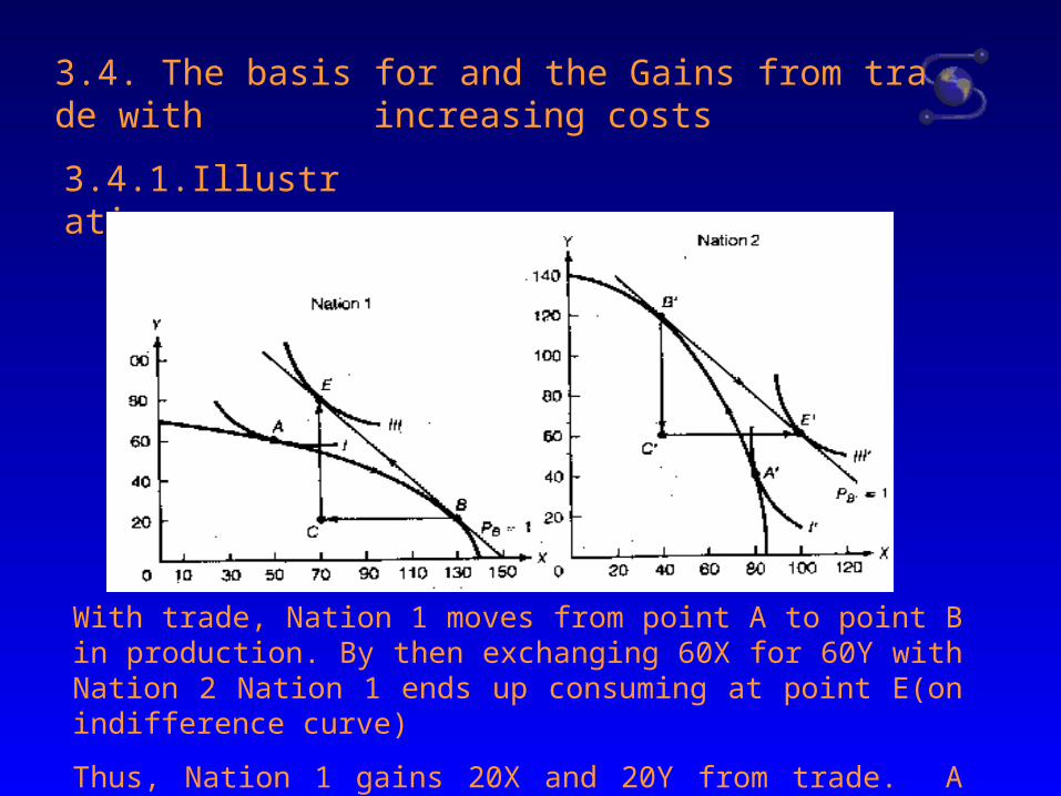
3.4. The basis for and the Gains from trade with increasing costs

3.4.1.Illustrations

With trade, Nation 1 moves from point A to point B in production. By then exchanging 60X for 60Y with Nation 2 Nation 1 ends up consuming at point E(on indifference curve)

Thus, Nation 1 gains 20X and 20Y from trade. A ---- E

A.   With trade, each nation specializes in producing the commodity of its comparative advantage and faces in creasing opportunity costs.

B.   Specialization in production proceeds until relative commodity prices in the two nations are equalized at the level at which trade is in equilibrium.

3.4.2. Equilibrium relative Commodity Prices with trade

The process of specialization in production continues until relative commodity prices (the slope of the production frontiers) become equal in the two nations

PB = PB’

The equilibrium relative commodity price with trade is the common relative price in both nations at which trade is balanced

3.4.3. Incomplete Specialization

Under constant costs, both nations specialize completely in production of the commodity of their comparative advantage

Under increasing opportunity costs, there is incomplete specialization in production in both nations.

The reason for this is that as Nation 1 specializes in the production of X, it incurs increasing opportunity costs in producing X.

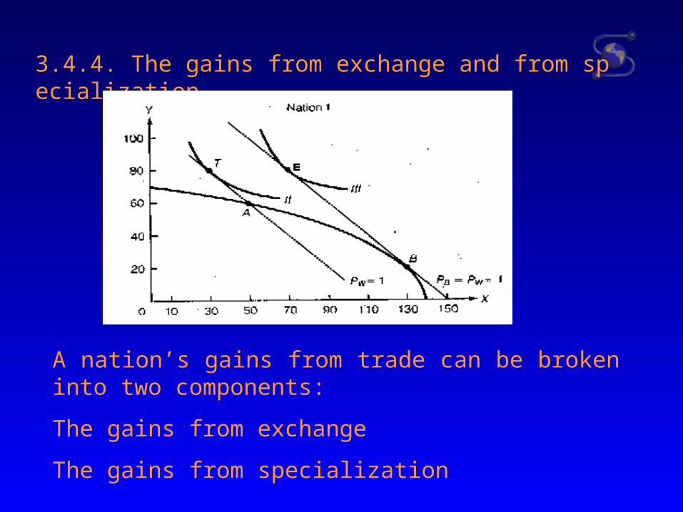
3.4.4. The gains from exchange and from specialization

A nation’s gains from trade can be broken into two components:

The gains from exchange

The gains from specialization

3.5. Trade based on differences in tastes

with increasing costs, even if two nations have identical production possibility frontiers (which is unlikely), there will still be a basis for mutually beneficial trade if tastes, or demand preferences, in the two nations differ.

The nation with the relatively smaller demand or preference for a commodity will have a lower autarky relative price for, and a comparative advantage in, that commodity.

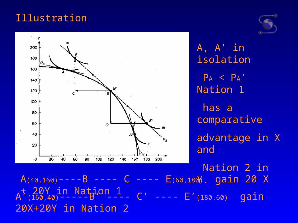
Illustration

A, A’ in isolation

PA < PA’ Nation 1

has a comparative

advantage in X and

Nation 2 in Y.

A(40,160)----B ---- C ---- E(60,180) gain 20 X + 20Y in Nation 1

A’(160,40)-----B’ ---- C’ ---- E’(180,60) gain 20X+20Y in Nation 2

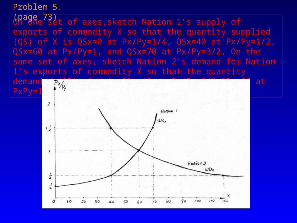
On one set of axes,sketch Nation 1’s supply of exports of commodity X so that the quantity supplied (QS) of X is QSx=0 at Px/Py=1/4, QSx=40 at Px/Py=1/2, QSx=60 at Px/Py=1, and QSx=70 at Px/Py=3/2, On the same set of axes, sketch Nation 2’s demand for Nation 1’s exports of commodity X so that the quantity demanded (QD) of X is QDx=40 at Px/Py=3/2,QDx=60 at PxPy=1, and QDx=120 at Px/Py=1/2

Problem 5. (page 73)

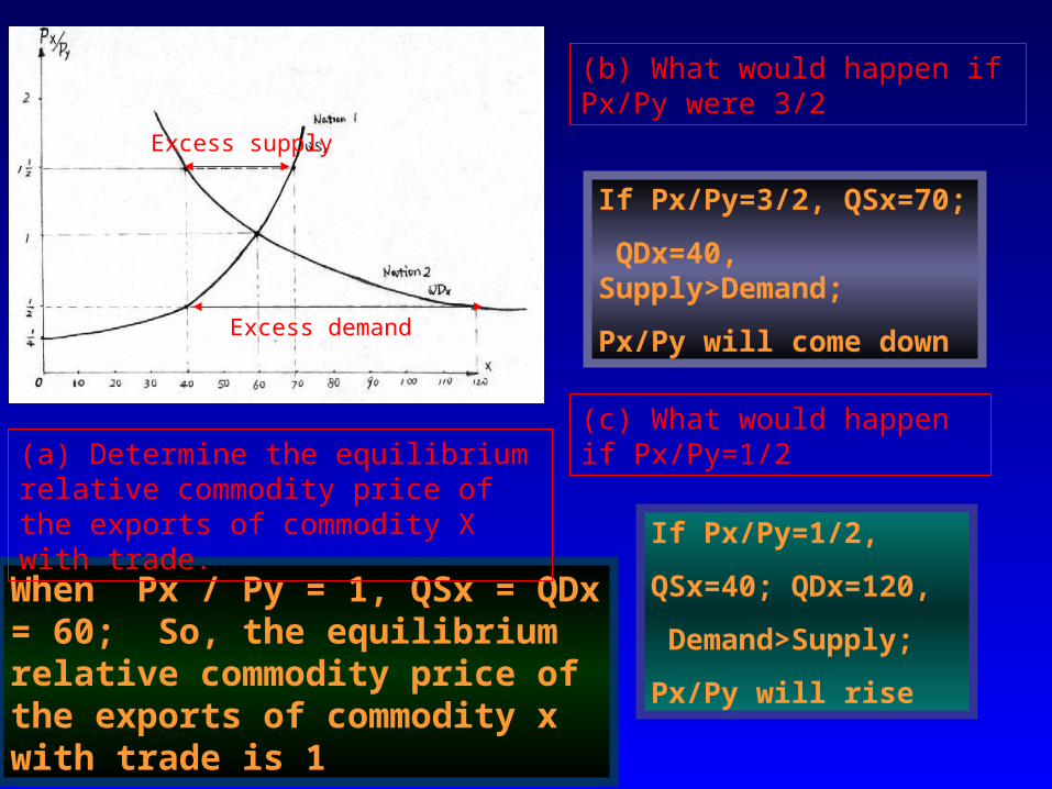
When Px / Py = 1, QSx = QDx = 60; So, the equilibrium relative commodity price of the exports of commodity x with trade is 1

If Px/Py=3/2, QSx=70;

QDx=40, Supply>Demand;

Px/Py will come down

If Px/Py=1/2,

QSx=40; QDx=120,

Demand>Supply;

Px/Py will rise

(a) Determine the equilibrium relative commodity price of the exports of commodity X with trade.

(b) What would happen if Px/Py were 3/2

(c) What would happen if Px/Py=1/2

Excess supply

Excess demand

Chapter 4 Demand and Supply, Offer Curves,

and the Terms of Trade

4.1 Theory of Reciprocal Demand

John Stuart Mill (1806-1873)

Essays on some Unsettled Questions of Political Economy (1844),

Principles of Political Economy (1848).

Main view on trade:

The actual price at which trade takes place depends on the trading partners’ interacting demands.

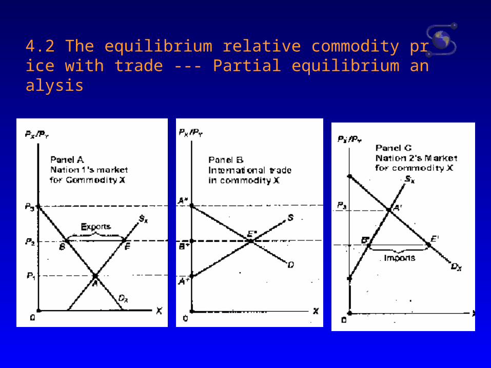
4.2 The equilibrium relative commodity price with trade --- Partial equilibrium analysis

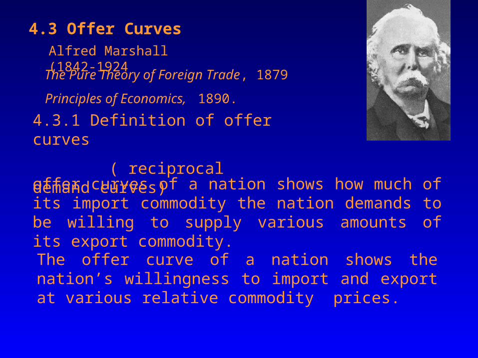
4.3 Offer Curves

offer curves of a nation shows how much of its import commodity the nation demands to be willing to supply various amounts of its export commodity.

The offer curve of a nation shows the nation’s willingness to import and export at various relative commodity prices.

4.3.1 Definition of offer curves

( reciprocal demand curves)

Alfred Marshall (1842-1924

The Pure Theory of Foreign Trade, 1879

Principles of Economics, 1890.

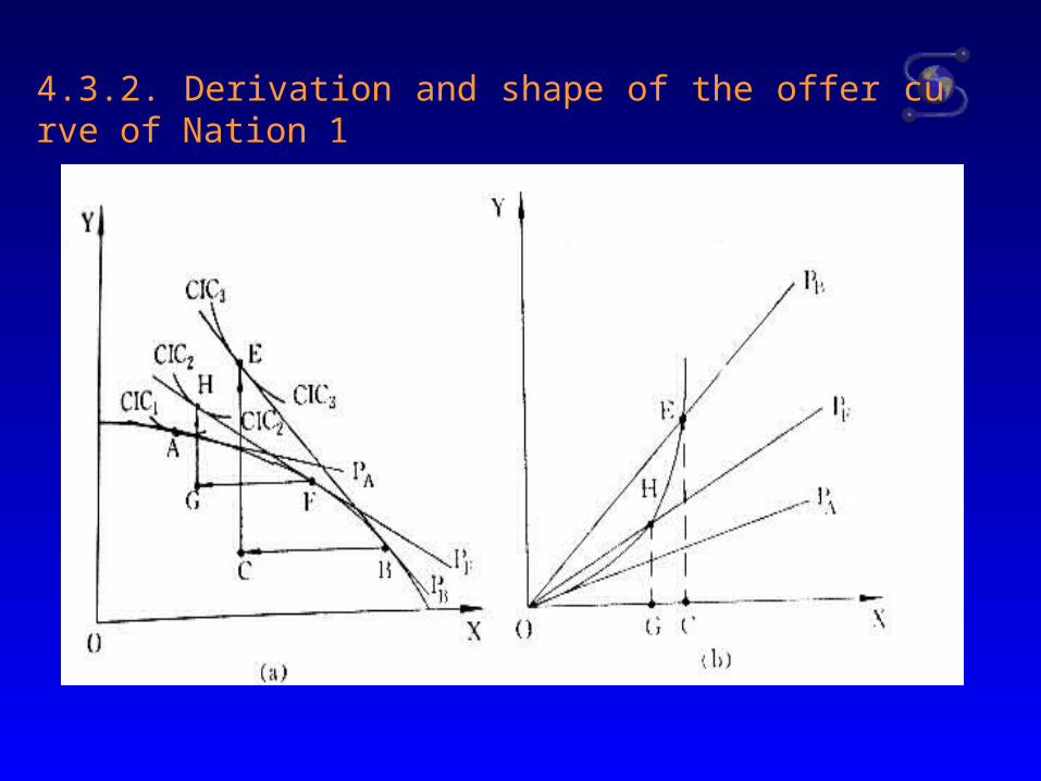
4.3.2. Derivation and shape of the offer curve of Nation 1

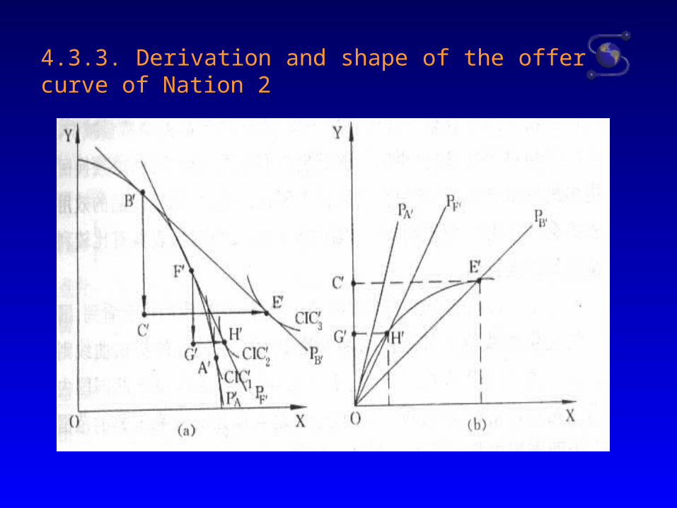
4.3.3. Derivation and shape of the offer curve of Nation 2

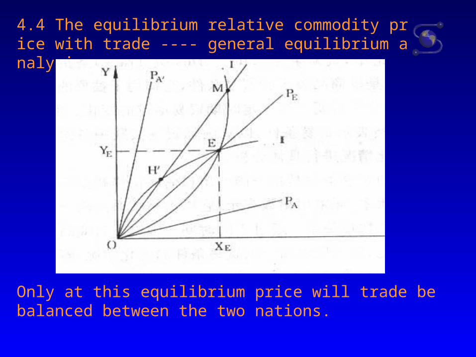
4.4 The equilibrium relative commodity price with trade ---- general equilibrium analysis

Only at this equilibrium price will trade be balanced between the two nations.

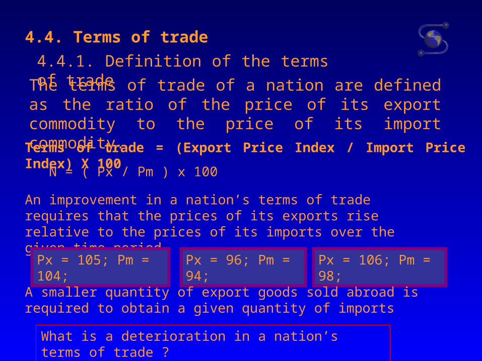
4.4. Terms of trade

4.4.1. Definition of the terms of trade

The terms of trade of a nation are defined as the ratio of the price of its export commodity to the price of its import commodity.

Terms of trade = (Export Price Index / Import Price Index) X 100

N = ( Px / Pm ) x 100

An improvement in a nation’s terms of trade requires that the prices of its exports rise relative to the prices of its imports over the given time period.

Px = 105; Pm = 104; Px = 96; Pm = 94; Px = 106; Pm = 98;

A smaller quantity of export goods sold abroad is required to obtain a given quantity of imports

What is a deterioration in a nation’s terms of trade ?

Country Export

Price index

Import

Price index

Terms of

Trade

Japan

United States

United kingdom

Germany

Canada

Australia

145

109

113

108

101

94

105

106

113

109

103

110

138

103

100

99

98

85

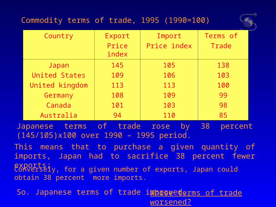
Commodity terms of trade, 1995 (1990=100)

Japanese terms of trade rose by 38 percent (145/105)x100 over 1990 – 1995 period.

This means that to purchase a given quantity of imports, Japan had to sacrifice 38 percent fewer exports;

Conversely, for a given number of exports, Japan could obtain 38 percent more imports.

So. Japanese terms of trade improved. Whose terms of trade worsened?

Chapter 5 Factor Endowments and the( 要素禀赋说）

Heckscher-Ohlin Theory （赫克雪尔 - 俄林定理）

(Trade Model Extensions and applications)

5.1 introduction

In 1919, Heckscher published “The Effect of Foreign Trade on the Distribution of Income”

In 1933 Ohlin published “Interregional and International Trade”

Ohlin was awarded the 1977 Nobel prize in economics for his contribution to the theory of international trade.

5.2. Assumptions of the theory

 (1) two nations, two commodities (X,Y), and two factors of

production (labor ,capital)

   (2) Both nations use the same technology in production;

(3) The same commodity is labor intensive in both nations

X --- labor intensive ;Y---- capital intensive

(4) Constant returns to scale;

(5) Incomplete specialization in production;

(6) Equal tastes in both nations;

(8) Perfect internal but no international mobility of factor;

(7) Perfect competition in both commodities and factor

markets;

(9) No transportation costs, tariffs, or other obstructions

to the free flow of international trade;

(10) All resources are fully employed;

(11) Trade is balanced.

5.3 Factor intensity, Factor abundance,

and the shape of the production frontier

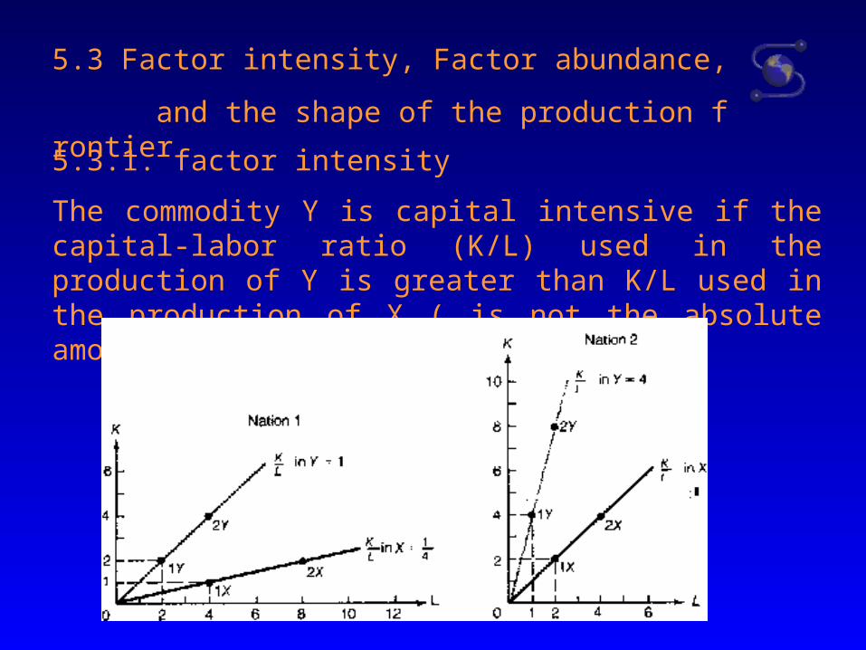
5.3.1. factor intensity

The commodity Y is capital intensive if the capital-labor ratio (K/L) used in the production of Y is greater than K/L used in the production of X ( is not the absolute amount of K and L.)

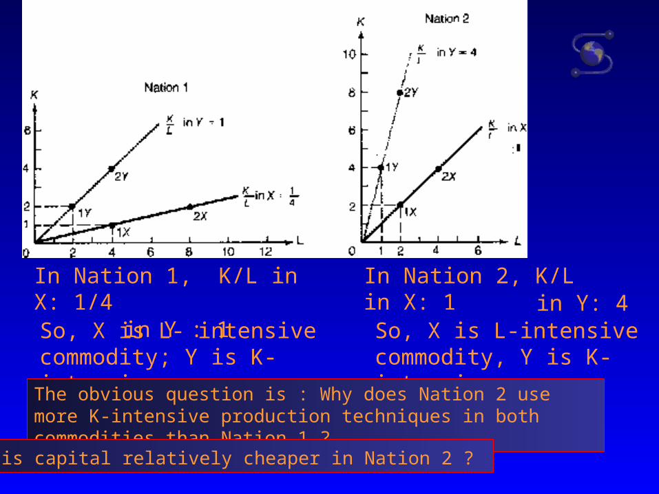
In Nation 1, K/L in X: 1/4 in Y : 1

So, X is L- intensive commodity; Y is K-intensive

In Nation 2, K/L in X: 1 in Y: 4

So, X is L-intensive commodity, Y is K-intensive

The obvious question is : Why does Nation 2 use more K-intensive production techniques in both commodities than Nation 1 ?

Why is capital relatively cheaper in Nation 2 ?

5.3.2. Factor abundance

  a. In terms of physical units : the overall amount of capital and labor available to each nation. The ratio of the total amount of capital to the total amount of labor.

Nation 2 is capital abundant if TK2/TL2 > TK1/TL1

b. In terms of relative factor prices: the rental price of capital and the price of labor time in each nation. The ratio of the rental price of capital to the price of labor time

Pk/PL= r/w r: interest rate; w: wage rate

Nation 2 is capital abundant if PK2/PL2 < PK1/PL1 or r2/w2 < r1/w1

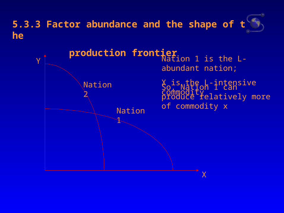
5.3.3 Factor abundance and the shape of the

production frontier

Y

X

Nation 1

Nation 1 is the L-abundant nation;

X is the L-intensive commodity

Nation 2 So, Nation 1 can produce relatively more of commodity x

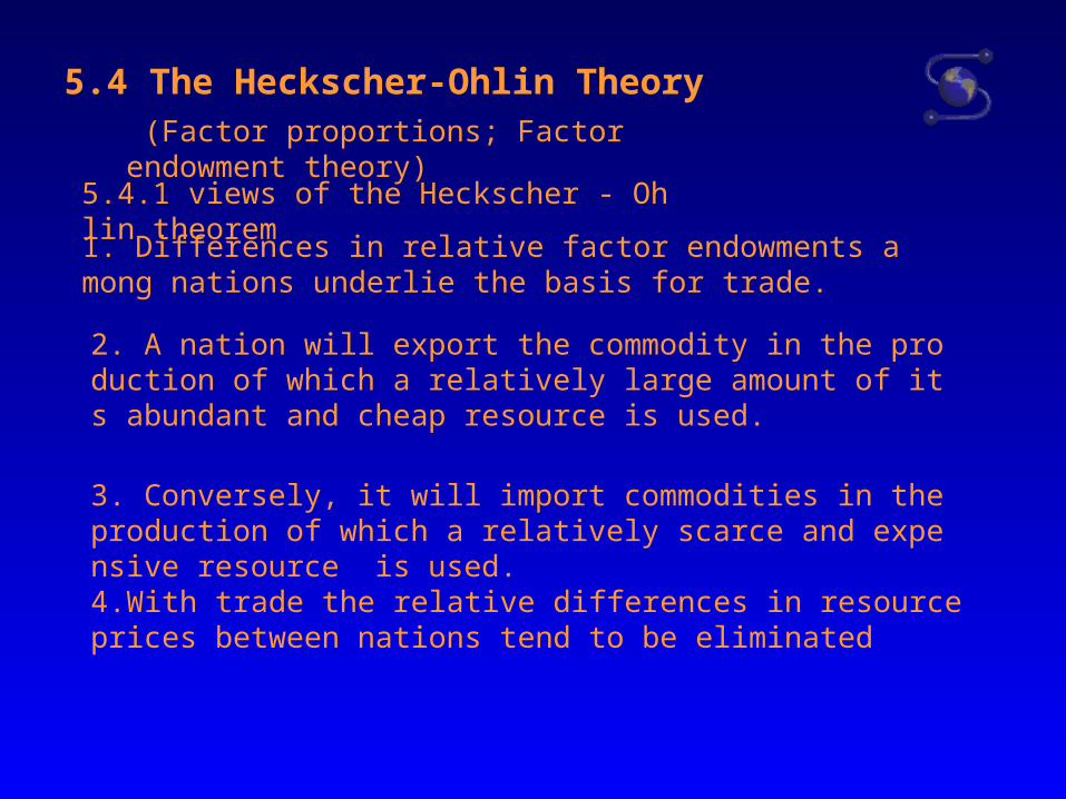
5.4 The Heckscher-Ohlin Theory

1. Differences in relative factor endowments among nations underlie the basis for trade.

2. A nation will export the commodity in the production of which a relatively large amount of its abundant and cheap resource is used.

3. Conversely, it will import commodities in the production of which a relatively scarce and expensive resource is used.

4.With trade the relative differences in resource prices between nations tend to be eliminated

(Factor proportions; Factor endowment theory)

5.4.1 views of the Heckscher - Ohlin theorem

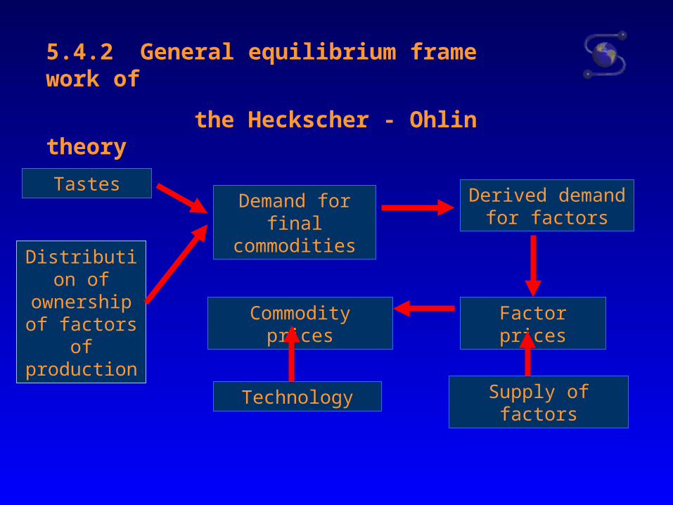
5.4.2 General equilibrium framework of

the Heckscher - Ohlin theory

Tastes

Distribution of ownership of

factors of production

Demand for final commodities

Derived demand for factors

Factor prices

Supply of factors

Commodity prices

Technology

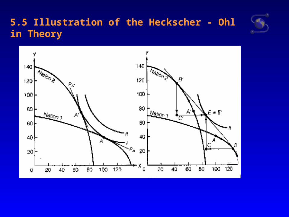
5.5 Illustration of the Heckscher - Ohlin Theory

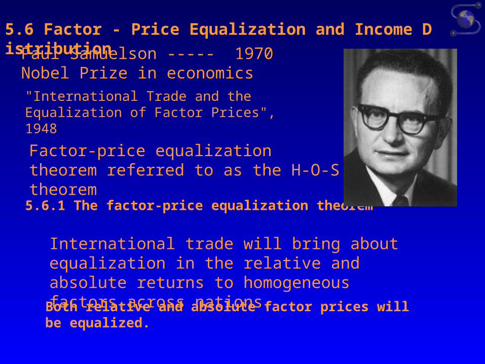
5.6 Factor - Price Equalization and Income Distribution

Paul Samuelson ----- 1970 Nobel Prize in economics

Factor-price equalization theorem referred to as the H-O-S theorem

5.6.1 The factor-price equalization theorem

International trade will bring about equalization in the relative and absolute returns to homogeneous factors across nations.

Both relative and absolute factor prices will be equalized.

"International Trade and the Equalization of Factor Prices", 1948

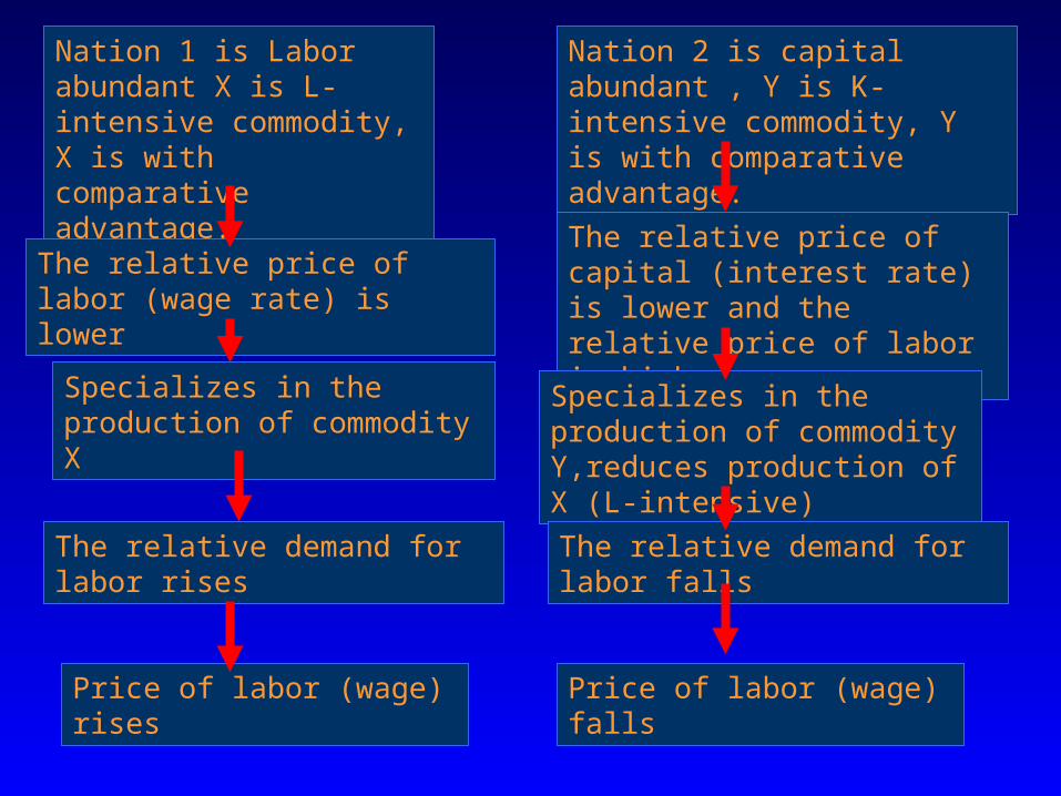
Nation 1 is Labor abundant X is L-intensive commodity, X is with comparative advantage.

The relative price of labor (wage rate) is lower

Specializes in the production of commodity X

The relative demand for labor rises

Price of labor (wage) rises

Nation 2 is capital abundant , Y is K-intensive commodity, Y is with comparative advantage.

The relative price of capital (interest rate) is lower and the relative price of labor is higher

Specializes in the production of commodity Y,reduces production of X (L-intensive)

The relative demand for labor falls

Price of labor (wage) falls

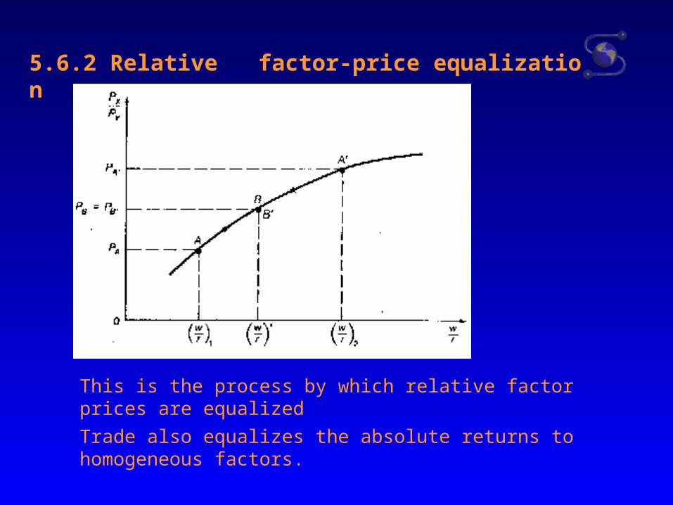
5.6.2 Relative factor-price equalization

This is the process by which relative factor prices are equalized

Trade also equalizes the absolute returns to homogeneous factors.

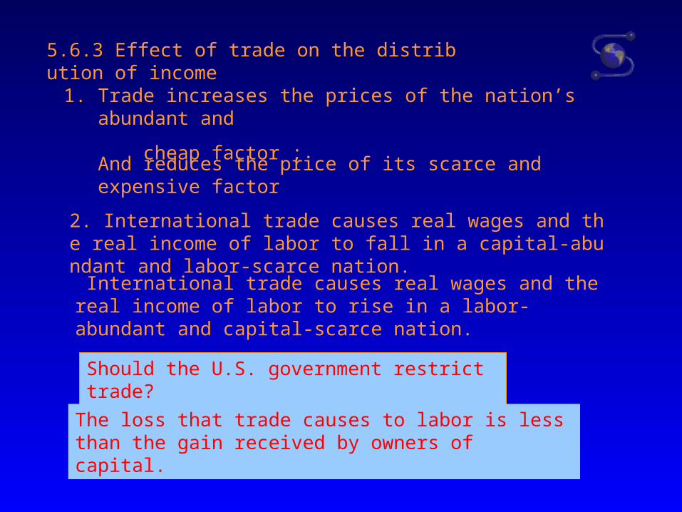
5.6.3 Effect of trade on the distribution of income

1. Trade increases the prices of the nation’s abundant and

cheap factor ;

And reduces the price of its scarce and expensive factor

2. International trade causes real wages and the real income of labor to fall in a capital-abundant and labor-scarce nation.

International trade causes real wages and the real income of labor to rise in a labor-abundant and capital-scarce nation.

Should the U.S. government restrict trade?

The loss that trade causes to labor is less than the gain received by owners of capital.

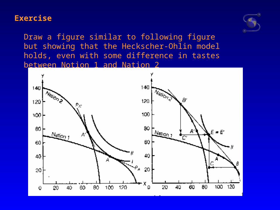
Draw a figure similar to following figure but showing that the Heckscher-Ohlin model holds, even with some difference in tastes between Notion 1 and Nation 2

Exercise

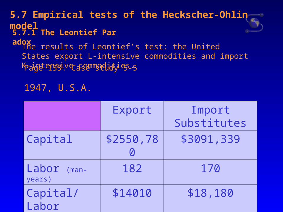
5.7 Empirical tests of the Heckscher-Ohlin model

5.7.1 The Leontief Paradox

The results of Leontief’s test: the United States export L-intensive commodities and import K-intensive commodities.

Page 133. Case study 5-5

Export Import Substitutes

Capital $2550,780 $3091,339

Labor (man-years) 182 170

Capital/Labor $14010 $18,180

1947, U.S.A.

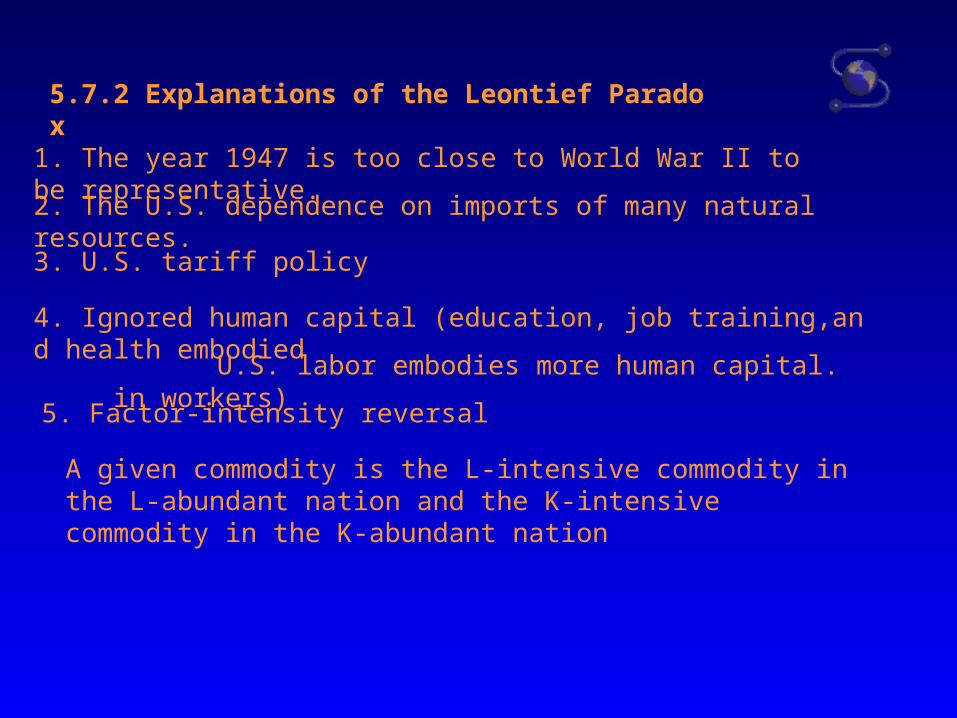
5.7.2 Explanations of the Leontief Paradox

1. The year 1947 is too close to World War II to be representative.

2. The U.S. dependence on imports of many natural resources.

3. U.S. tariff policy

4. Ignored human capital (education, job training,and health embodied

in workers) U.S. labor embodies more human capital.

5. Factor-intensity reversal

A given commodity is the L-intensive commodity in the L-abundant nation and the K-intensive commodity in the K-abundant nation

Chapter 6 New International Trade Theories

6.1 Theory of Increasing Returns to scale

(1).There is still a basis for mutually beneficial trade based on economies of scale, even if two nations are identical in every respect.

(2) When economies of scale are present, total world output of both commodities will be greater than without specialization

(3) With trade, each nation then shares in these gains.

6.1.1 Main views

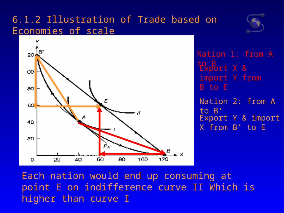
6.1.2 Illustration of Trade based on Economies of scale

Nation 1: from A to B

Export X & import Y from B to E

Nation 2: from A to B’

Export Y & import X from B’ to E

Each nation would end up consuming at point E on indifference curve II Which is higher than curve I

6.2 Intra-Industry Trade theory

(Differentiated Product Theory)

Intra-industry trade refers to the exchange between nations of differentiated products of the same industry .

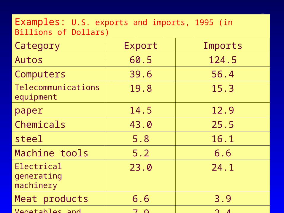
Examples: U.S. exports and imports, 1995 (in Billions of Dollars)

Category Export Imports

Autos 60.5 124.5

Computers 39.6 56.4Telecommunications equipment

19.8 15.3

paper 14.5 12.9

Chemicals 43.0 25.5

steel 5.8 16.1

Machine tools 5.2 6.6Electrical generating machinery

23.0 24.1

Meat products 6.6 3.9Vegetables and fruits 7.9 2.4

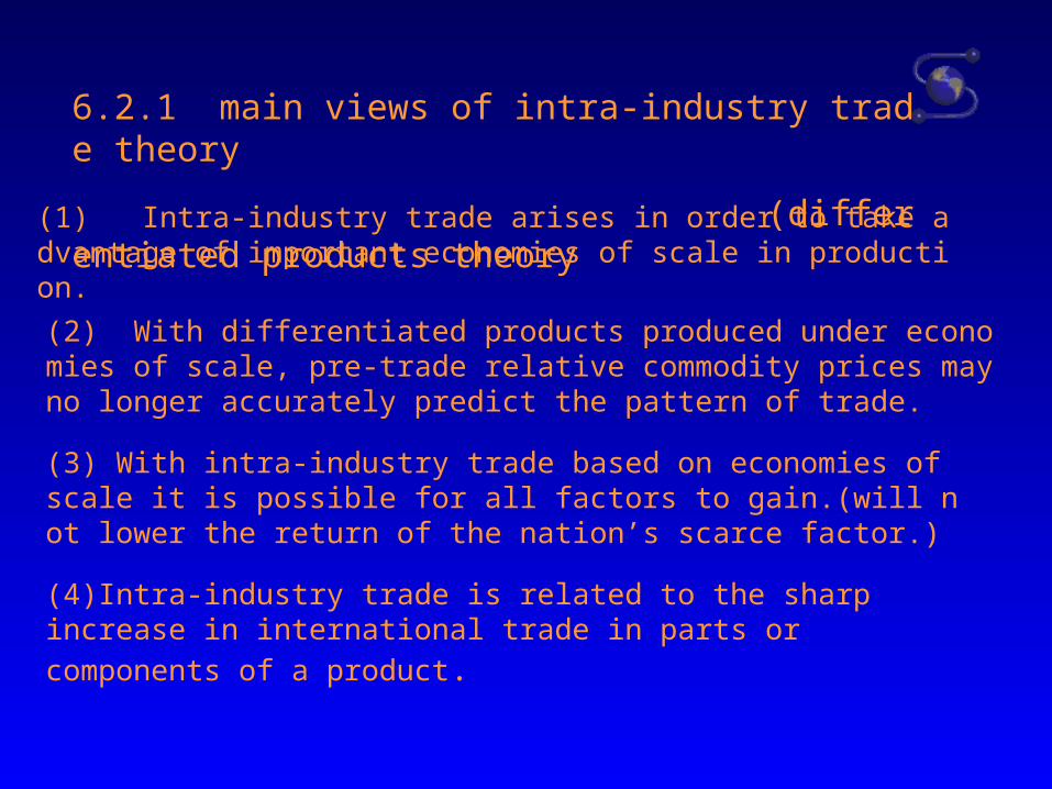
(1) Intra-industry trade arises in order to take advantage of important economies of scale in production.

(2) With differentiated products produced under economies of scale, pre-trade relative commodity prices may no longer accurately predict the pattern of trade.

(3) With intra-industry trade based on economies of scale it is possible for all factors to gain.(will not lower the return of the nation’s scarce factor.)

(4)Intra-industry trade is related to the sharp increase in international

trade in parts or components of a product.

6.2.1 main views of intra-industry trade theory

(differentiated products theory

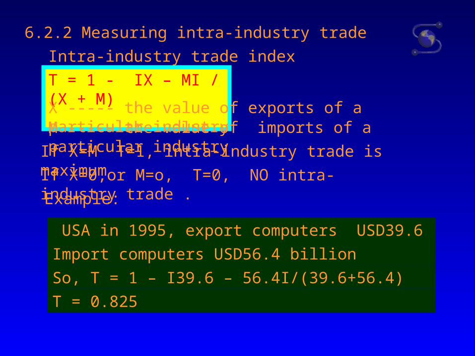
6.2.2 Measuring intra-industry trade

Intra-industry trade index ( T )

T = 1 - IX – MI / (X + M) X ----- the value of exports of a particular industryM ----- the value of imports of a particular industry

If X=M T=1, intra-industry trade is maximum

If X=0,or M=o, T=0, NO intra-industry trade .

USA in 1995, export computers USD39.6 billion

Import computers USD56.4 billion

So, T = 1 – I39.6 – 56.4I/(39.6+56.4)

T = 0.825

Example:

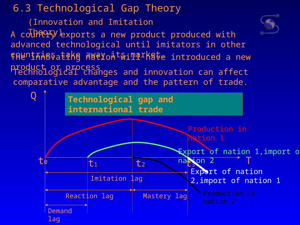
6.3 Technological Gap Theory(Innovation and Imitation Theory)

A country exports a new product produced with advanced technological until imitators in other countries take away its market.

T

Q

t0 t1 t2 t3

Production in nation 1

Export of nation 1,import of nation 2

Export of nation 2,import of nation 1

Demand lag

Reaction lag Production in nation 2

Imitation lag

Mastery lag

Technological gap and international trade

The innovating nation will have introduced a new product or processTechnological changes and innovation can affect comparative advantage and the pattern of trade.

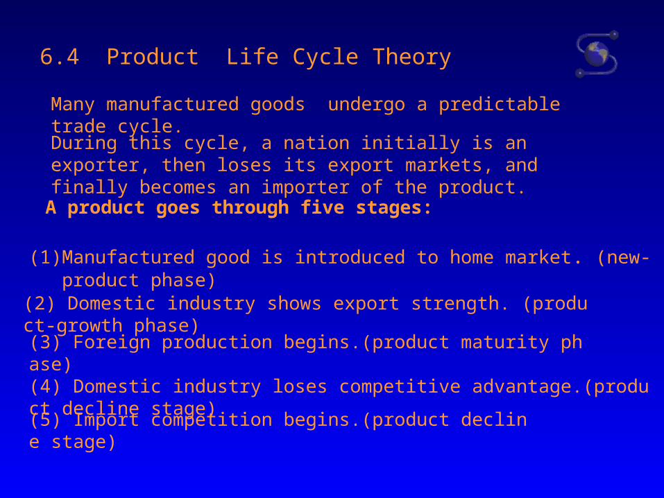
6.4 Product Life Cycle Theory

A product goes through five stages:

Many manufactured goods undergo a predictable trade cycle.

During this cycle, a nation initially is an exporter, then loses its export markets, and finally becomes an importer of the product.

(1) Manufactured good is introduced to home market. (new-product phase)

(2) Domestic industry shows export strength. (product-growth phase)

(3) Foreign production begins.(product maturity phase)

(4) Domestic industry loses competitive advantage.(product decline stage)

(5) Import competition begins.(product decline stage)

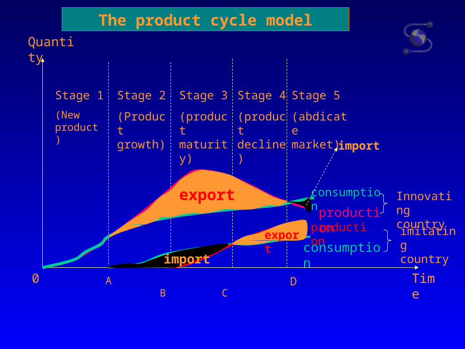
production

Stage 1

(New product)

Stage 2

(Product growth)

Stage 3

(product maturity)

Stage 4

(product decline)

Stage 5

(abdicate market)

Time

Quantity

0 A B C D

consumption

consumption

Innovating country

production imitating country

export

import

import

export

The product cycle model

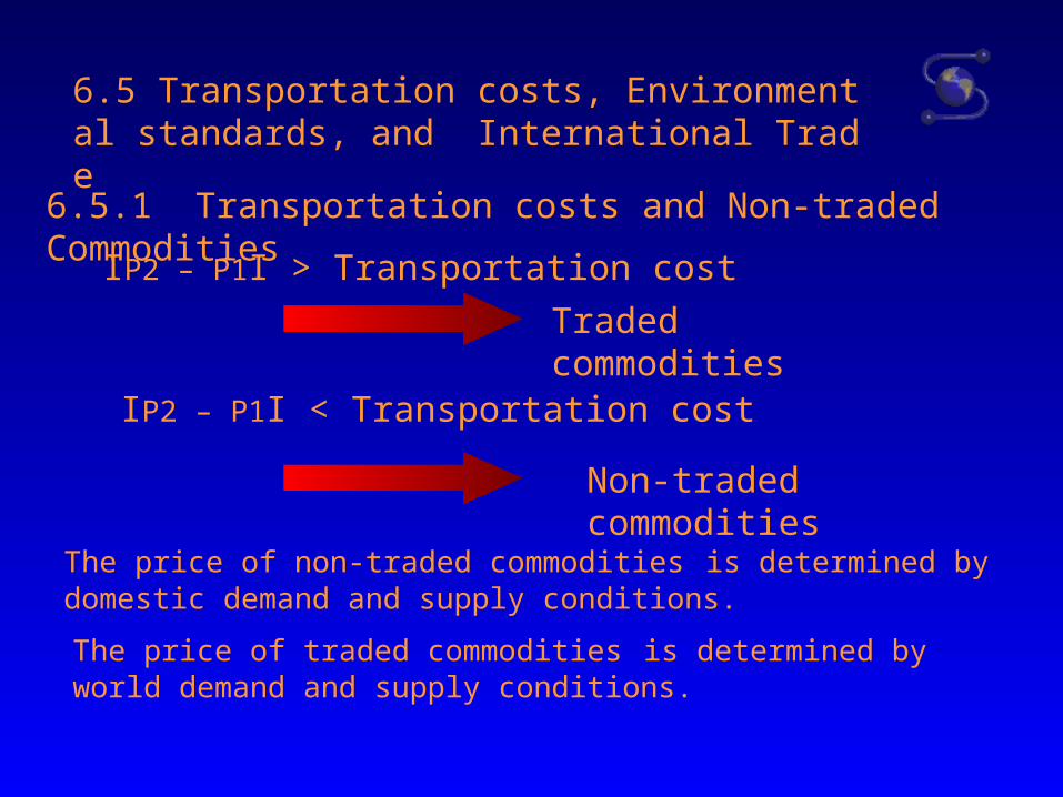
6.5 Transportation costs, Environmental standards, and International Trade

6.5.1 Transportation costs and Non-traded Commodities

IP2 – P1I > Transportation cost

Traded commodities

IP2 – P1I < Transportation cost

Non-traded commodities

The price of non-traded commodities is determined by domestic demand and supply conditions.

The price of traded commodities is determined by world demand and supply conditions.

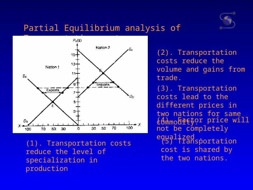
Partial Equilibrium analysis of Transportation cost

(1). Transportation costs reduce the level of specialization in production

(2). Transportation costs reduce the volume and gains from trade.

(3). Transportation costs lead to the different prices in two nations for same commodity.

(4). Factor price will not be completely equalized .

(5) Transportation cost is shared by the two nations.

6.5.2 Transportation Costs and the Location of Industry

Resource-oriented industries

Market-oriented industries

Footloose industries

6.5.3 Environmental standards, Industry Location,

and international Trade

Alexander Hamilton (1755-1804) 汉密尔顿 7.1 The theory of protective tariff

He recommended specific policies to encourage manufactures:

“Report on Manufactures” - submitted to Congress 1791

protective duties

prohibitions on rival imports

exemption of domestic manufactures from duties

encouragement of "new inventions . . . particularly those, which relate to machinery."

Chapter 7 The Theory of Protective Trade

List, (Georg) Friedrich ( 1789 --- 1846) ( 李斯特）German-U.S. economist

His best-known work was

The National System of Political Economy (1841).

He maintained that a national economy in an early stage of industrialization required tariff protection to stimulate development

Political Economy (1827)

He first gained prominence as the founder of an association of German industrialists that favored abolishing tariff barriers between the German states

7.2 The theory of protecting infant industry

7.3 The theory of foreign trade multiplier

7.3.1 Determination of the equilibrium national income

in a closed economy

Gross National Product (GNP)Total final value of goods and services produced in a national economy over a particular period of time,usually one year.National income (Y)The sum of all payments made to sum factors of production.

John Maynard Keynes (1883 – 1946)

“The General Theory of Employment, Interest and Money”《就业、利息和货币通论》

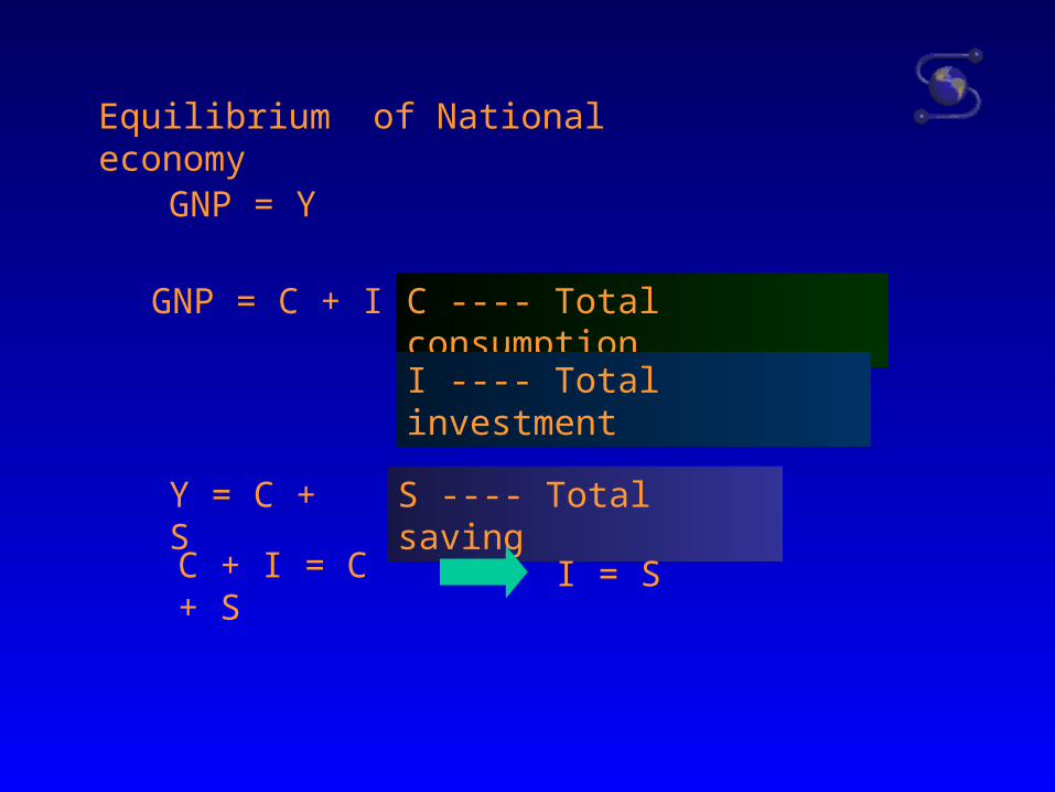
Equilibrium of National economy

GNP = Y

GNP = C + I C ---- Total consumption

I ---- Total investment

Y = C + S S ---- Total saving

C + I = C + S I = S

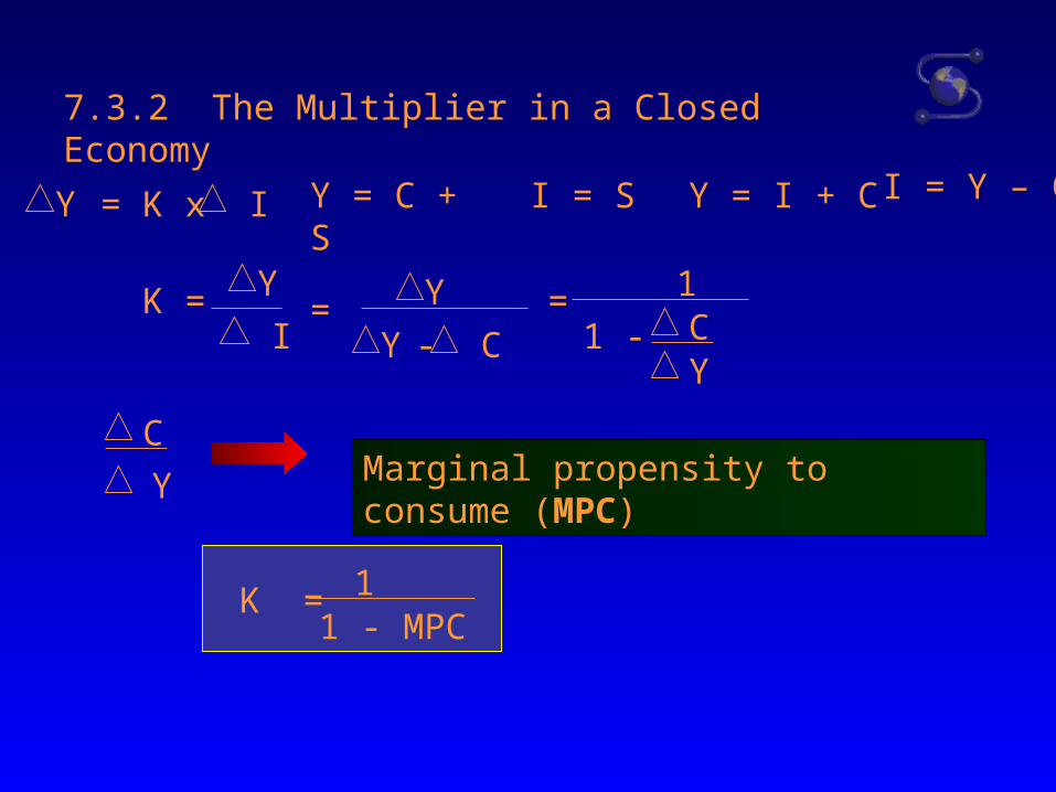
7.3.2 The Multiplier in a Closed Economy

Y = K x I

Y

IK = = Y

Y - C = 1

1 - CY

C

Y Marginal propensity to consume (MPC)

K = 11 - MPC

Y = C + S I = S Y = I + C I = Y – C

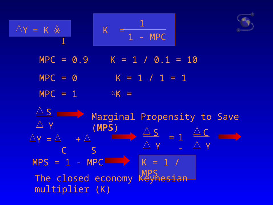
K = 1

1 - MPC

MPC = 0.9 K = 1 / 0.1 = 10

MPC = 0 K = 1 / 1 = 1

MPC = 1 K =

Y = K x I

Marginal Propensity to Save (MPS)

Y = C + S

S

Y1 - S

Y= C

Y

MPS = 1 - MPC K = 1 / MPS

The closed economy Keynesian multiplier (K)

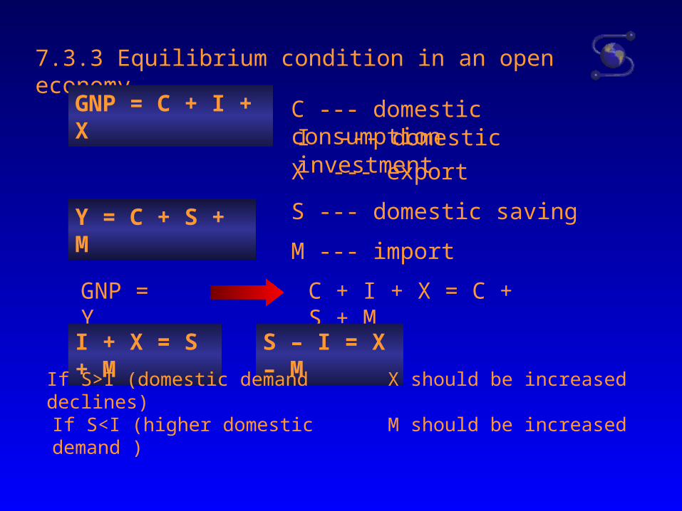
7.3.3 Equilibrium condition in an open economy

GNP = C + I + X C --- domestic consumptionI --- domestic investment

X --- export

Y = C + S + M S --- domestic saving

M --- import

GNP = Y C + I + X = C + S + M

I + X = S + M S – I = X – M

If S>I (domestic demand declines) X should be increased

If S<I (higher domestic demand ) M should be increased

7.3.4 The foreign trade multiplier

I + X = S + M

I + X = S + M

Y )S = (MPS) (S= MPS

Y

M= MPM

YM = (MPM) ( Y )

Marginal Propensity to Save

Marginal Propensity to import

…….(1)

….. (2)

….. (3)

I + X = Y (MPS +MPM)

Y = 1

MPS + MPM I + X( )

Foreign trade multiplier (K’) is 1

MPS + MPM

I + X = S + M

I + X - M = S

SMPS = Y

Y = S MPS

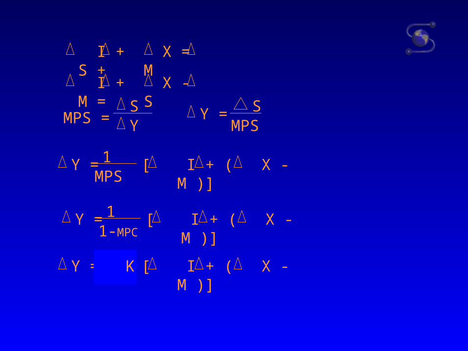
I + ( X - M )]Y = 1MPS

[

I + ( X - M )]Y = 11-MPC

[

I + ( X - M )]Y = 11-MPC

[K

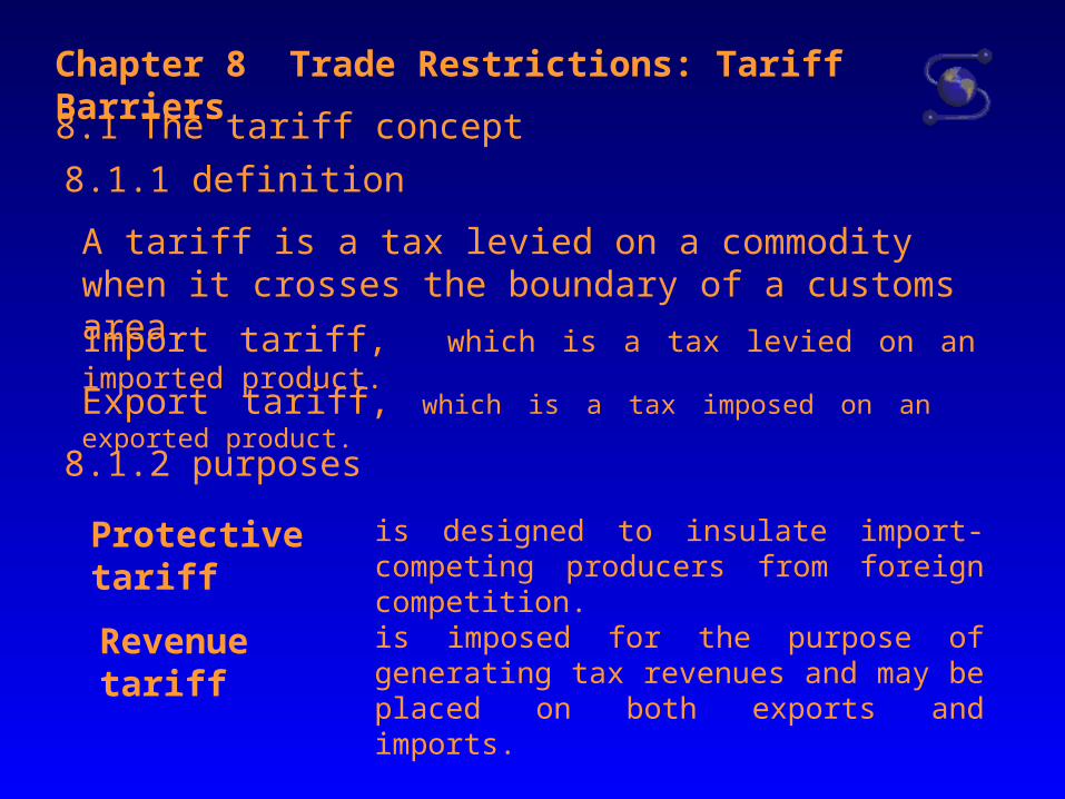
Chapter 8 Trade Restrictions: Tariff Barriers

8.1 The tariff concept

8.1.1 definition

A tariff is a tax levied on a commodity when it crosses the boundary of a customs area.

Import tariff, which is a tax levied on an imported product.

Export tariff, which is a tax imposed on an exported product.

8.1.2 purposes

Protective tariff is designed to insulate import-competing producers from foreign competition.

Revenue tariff is imposed for the purpose of generating tax revenues and may be placed on both exports and imports.

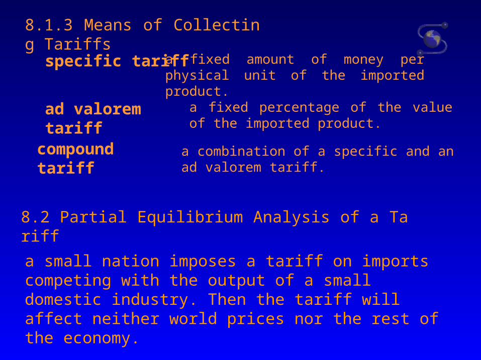
8.1.3 Means of Collecting Tariffs

specific tariff a fixed amount of money per physical unit of the imported product.

ad valorem tariff a fixed percentage of the value of the imported product.

compound tariff a combination of a specific and an ad valorem tariff.

8.2 Partial Equilibrium Analysis of a Tariff

a small nation imposes a tariff on imports competing with the output of a small domestic industry. Then the tariff will affect neither world prices nor the rest of the economy.

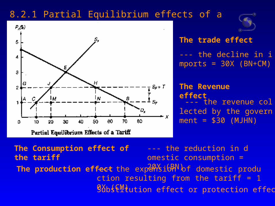
8.2.1 Partial Equilibrium effects of a Tariff

The Consumption effect of the tariff --- the reduction in domestic consumption = 20X (BN)

The production effect --- the expansion of domestic production resulting from the tariff = 10X (CM)

The trade effect

--- the decline in imports = 30X (BN+CM)

The Revenue effect

--- the revenue collected by the government = $30 (MJHN)

Substitution effect or protection effect

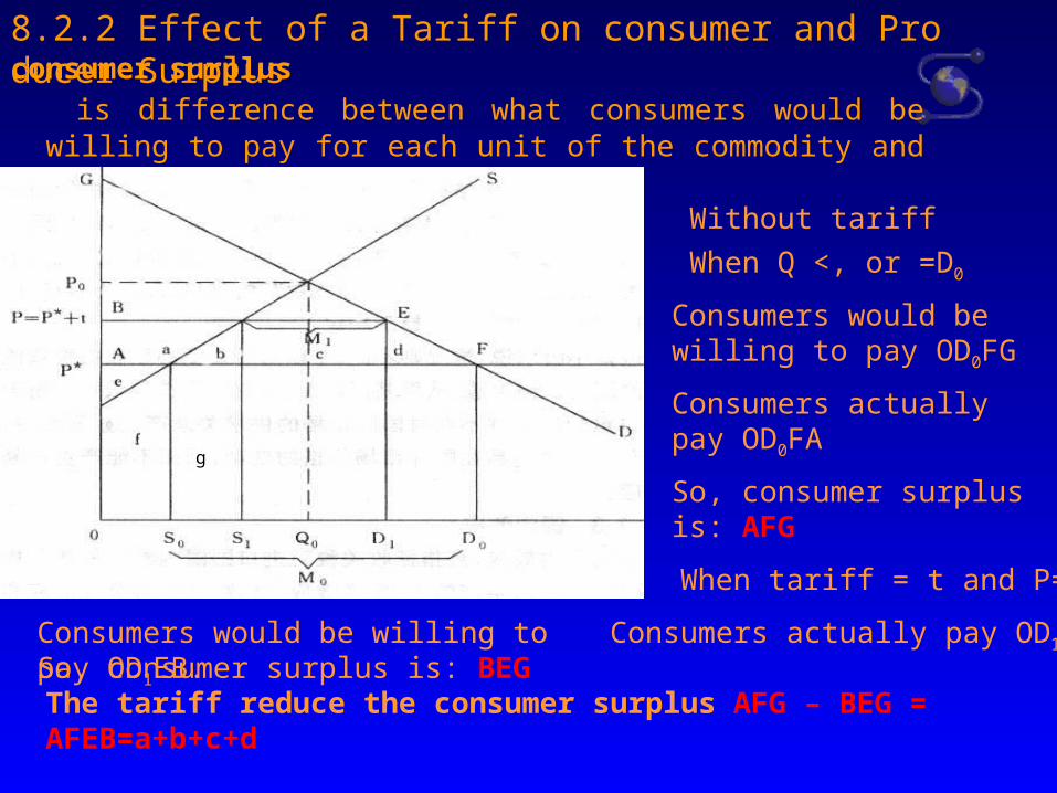
8.2.2 Effect of a Tariff on consumer and Producer Surplus consumer surplus

is difference between what consumers would be willing to pay for each unit of the commodity and what they actually pay

When Q <, or =D0

Consumers would be willing to pay OD0FG

Consumers actually pay OD0FA

Without tariff

So, consumer surplus is: AFG

When tariff = t and P=P*+t

Consumers would be willing to pay OD1EB.So, consumer surplus is: BEGThe tariff reduce the consumer surplus AFG – BEG = AFEB=a+b+c+d

Consumers actually pay OD1EB

g

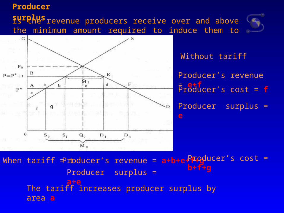
Producer surplus is the revenue producers receive over and above the minimum amount required to induce them to supply the goods (profit)

The tariff increases producer surplus by area a

Without tariff

Producer’s revenue = a+b+e+f+g

Producer’s cost = f

Producer surplus = e

When tariff = t

g

Producer’s revenue = e+f

Producer’s cost = b+f+g

Producer surplus = a+e

8.3 The degree of protection afforded by a tariff

8.3.1 Tariff Level

  Tariff Level = Amount of Import tariff / Amount of import x100%

   Tariff Level = ∑C / ∑P = ∑(PxR) / ∑P

8.3.2 Nominal Rate of Protection --- NRP

NRP = (Pd – Pa) / Pa

Pd: the price of a commodity in domestic market

Pa : The price of a commodity in abroad market

NRP = tariff rate of the final commodity = t

(without considering the effect of exchange rate)

8.3.3 Effective Rate of Protection --- ERP

ERP indicates how much protection is actually provided to the domestic processing of the import competing commodity

ERP signifies the total increase in domestic productive activities (value added) that an existing tariff structure makes possible, compared with what would occur under free-trade conditions.

ERP =(V’ – V) / V

V’: value added in domestic productive activities

V: value added in abroad, free trade conditions

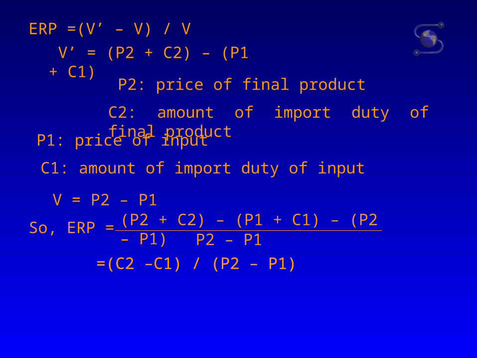
ERP =(V’ – V) / V

V’ = (P2 + C2) – (P1 + C1)

P2: price of final product

C2: amount of import duty of final product

P1: price of input

C1: amount of import duty of input

V = P2 – P1

So, ERP = (P2 + C2) – (P1 + C1) – (P2 – P1)P2 – P1

=(C2 –C1) / (P2 – P1) =(C2 –C1) / (P2 – P1)

=

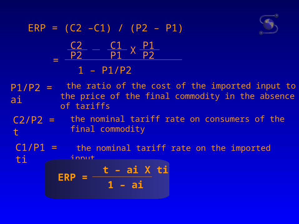
ERP = (C2 –C1) / (P2 – P1)

C2P2

C1P1

P1P2X

1 – P1/P2

P1/P2 = ai the ratio of the cost of the imported input to the price of the final commodity in the absence of tariffs

C2/P2 = t the nominal tariff rate on consumers of the final commodity

C1/P1 = ti the nominal tariff rate on the imported input

ERP = t – ai X ti

1 – ai

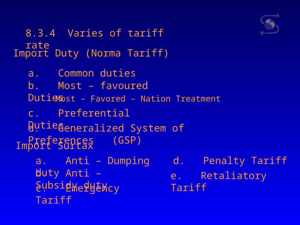
8.3.4 Varies of tariff rate

Import Duty (Norma Tariff)

a. Common duties

Most – Favored – Nation Treatment b. Most – favoured Duties

c. Preferential Duties

d. Generalized System of Preferences (GSP)

Import Surtax

a. Anti – Dumping dutyb. Anti – Subsidy duty

c. Emergency Tariff

d. Penalty Tariff

e. Retaliatory Tariff

Chapter 9 Non-tariff Trade Barriers and

the New Protectionism

9.1 Import quotas

a quota is the most important non-tariff trade barrier. It is a direct quantitative restriction on the amount of a commodity allowed to be imported or exported.

9.1.1 The effects of an import quota

Import quotas

---- used by all industrial nations to protect their agriculture

---- used by developing nations to stimulate import substitution of manufactured products and for balance-of-payments reasons.

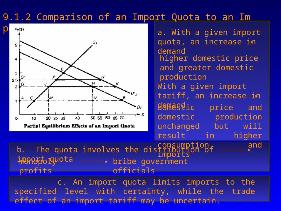
9.1.2 Comparison of an Import Quota to an Import Tariff

a. With a given import quota, an increase in demand

higher domestic price and greater domestic production

With a given import tariff, an increase in demand

domestic price and domestic production unchanged but will result in higher consumption and imports

b. The quota involves the distribution of import quota

monopoly profits bribe government officials

c. An import quota limits imports to the specified level with certainty, while the trade effect of an import tariff may be uncertain.

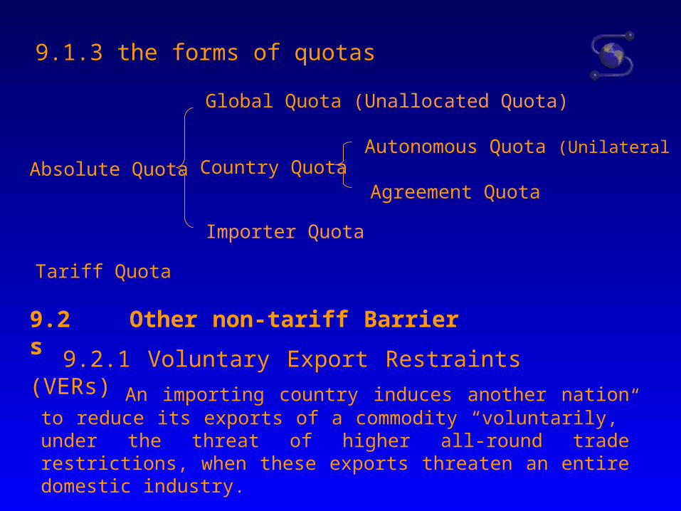
9.1.3 the forms of quotas

Absolute Quota

Tariff Quota

Global Quota (Unallocated Quota)

Country Quota Autonomous Quota (Unilateral Quota)

Agreement Quota

Importer Quota

9.2 Other non-tariff Barriers

9.2.1 Voluntary Export Restraints (VERs)

An importing country induces another nation to reduce its exports of a commodity “voluntarily,” under the threat of higher all-round trade restrictions, when these exports threaten an entire domestic industry.

9.2.2 Import License SystemOpen General License --- OGL

Specific License ---SL

9.2.3 Foreign Exchange control 9.2.4 Advanced Deposit 9.2.5 Minimum Price 9.2.6 Internal Taxes

9.2.7 State Monopoly (State trade) 9.2.8 Discriminatory Government Procurement Policy

9.2.9 Customs Procedures 9.2.10 Technical Barrier to Trade

technical standard

health and sanitary regulation

packing and labeling regulation

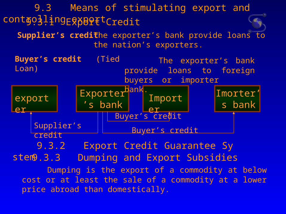
9.3 Means of stimulating export and controlling export

9.3.1 Export CreditSupplier’s credit

Buyer’s credit (Tied Loan)

exporter Exporter’s bank

Importer Imorter’s bank

Supplier’s creditBuyer’s credit

Buyer’s credit

9.3.2 Export Credit Guarantee System 9.3.3 Dumping and Export Subsidies

Dumping is the export of a commodity at below cost or at least the sale of a commodity at a lower price abroad than domestically.

The exporter’s bank provide loans to the nation’s exporters.

The exporter’s bank provide loans to foreign buyers or importer bank.

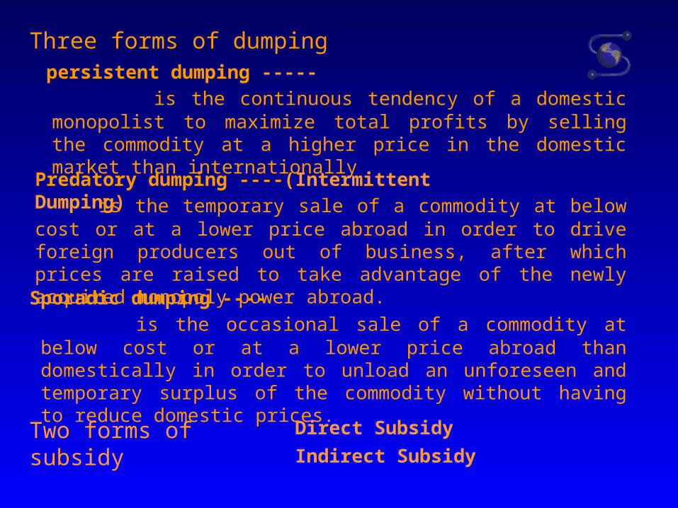
Direct Subsidy

Indirect Subsidy

Three forms of dumping persistent dumping -----

is the continuous tendency of a domestic monopolist to maximize total profits by selling the commodity at a higher price in the domestic market than internationally

Predatory dumping ----(Intermittent Dumping)

is the temporary sale of a commodity at below cost or at a lower price abroad in order to drive foreign producers out of business, after which prices are raised to take advantage of the newly acquired monopoly power abroad.

Sporadic dumping ----

is the occasional sale of a commodity at below cost or at a lower price abroad than domestically in order to unload an unforeseen and temporary surplus of the commodity without having to reduce domestic prices.

Two forms of subsidy

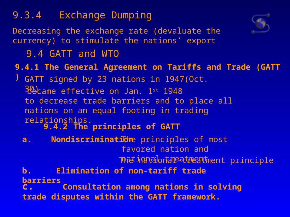
9.3.4 Exchange Dumping

Decreasing the exchange rate (devaluate the currency) to stimulate the nations’ export

9.4 GATT and WTO9.4.1 The General Agreement on Tariffs and Trade (GATT)

GATT signed by 23 nations in 1947(Oct. 30)

became effective on Jan. 1st 1948 to decrease trade barriers and to place all nations on an equal footing in trading relationships.

9.4.2 The principles of GATT

a. Nondiscrimination The principles of most favored nation and national treatment

The national-treatment principle b. Elimination of non-tariff trade barriers

c. Consultation among nations in solving trade disputes within the GATT framework.

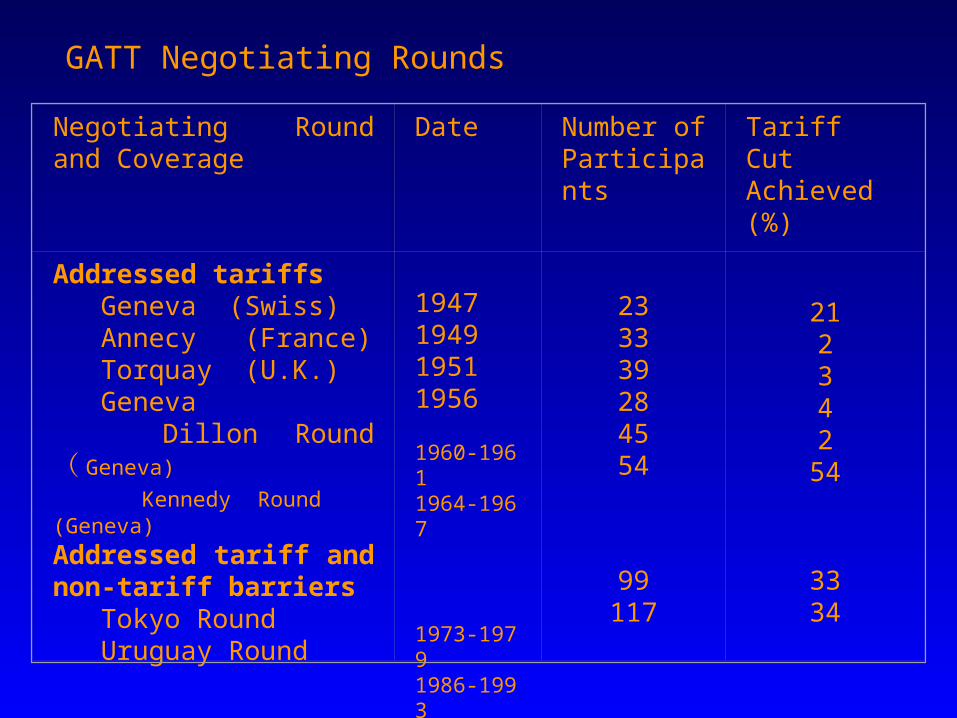
GATT Negotiating Rounds

Negotiating Round and Coverage

Date Number of Participants

Tariff CutAchieved (%)

Addressed tariffs Geneva (Swiss) Annecy (France) Torquay (U.K.) Geneva Dillon Round （ Geneva) Kennedy Round (Geneva)

Addressed tariff and non-tariff barriers Tokyo Round Uruguay Round 

1947194919511956

1960-19611964-1967 

1973-19791986-1993

 233339284554 

99117

 212342

54 

3334

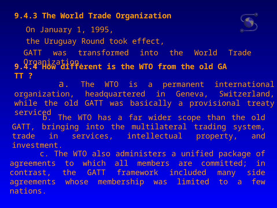
9.4.3 The World Trade Organization

On January 1, 1995,

the Uruguay Round took effect,

GATT was transformed into the World Trade Organization.

9.4.4 How different is the WTO from the old GATT ?

a. The WTO is a permanent international organization, headquartered in Geneva, Switzerland, while the old GATT was basically a provisional treaty serviced

b. The WTO has a far wider scope than the old GATT, bringing into the multilateral trading system, trade in services, intellectual property, and investment.

c. The WTO also administers a unified package of agreements to which all members are committed; in contrast, the GATT framework included many side agreements whose membership was limited to a few nations.

d. The WTO reverses policies of protection in certain “sensitive” areas (for example, agriculture and textiles) that were more or less tolerated in the old GATT.

e.  The WTO is not a government; individual nations retain their right to determine how they will make national laws conforming to their international obligations.

Chapter 10 Regional Economic Integration

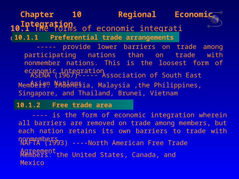
10.1 The forms of economic integration 10.1.1 Preferential trade arrangements

  ----- provide lower barriers on trade among participating nations than on trade with nonmember nations. This is the loosest form of economic integration

---- is the form of economic integration wherein all barriers are removed on trade among members, but each nation retains its own barriers to trade with nonmembers.

ASENA (1967)----- Association of South East Asian Nations

10.1.2 Free trade area

Members: Indonesia, Malaysia ,the Philippines, Singapore, and Thailand, Brunei, Vietnam

NAFTA (1993) ----North American Free Trade Agreement

Members: the United States, Canada, and Mexico

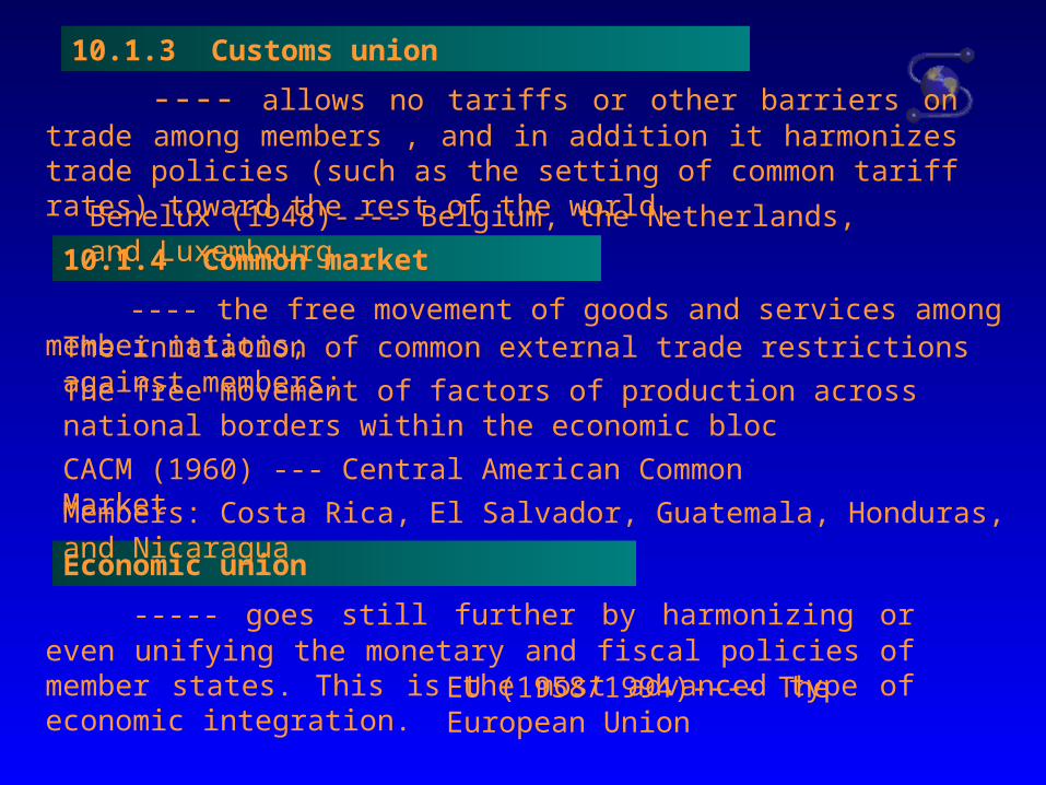
10.1.4 Common market

---- the free movement of goods and services among member nations;

Economic union

----- goes still further by harmonizing or even unifying the monetary and fiscal policies of member states. This is the most advanced type of economic integration.

10.1.3 Customs union

---- allows no tariffs or other barriers on trade among members , and in addition it harmonizes trade policies (such as the setting of common tariff rates) toward the rest of the world.

Benelux (1948)---- Belgium, the Netherlands, and Luxembourg

The initiation of common external trade restrictions against members;

The free movement of factors of production across national borders within the economic bloc

CACM (1960) --- Central American Common Market

Members: Costa Rica, El Salvador, Guatemala, Honduras, and Nicaragua

EU (1958/1994)---- The European Union

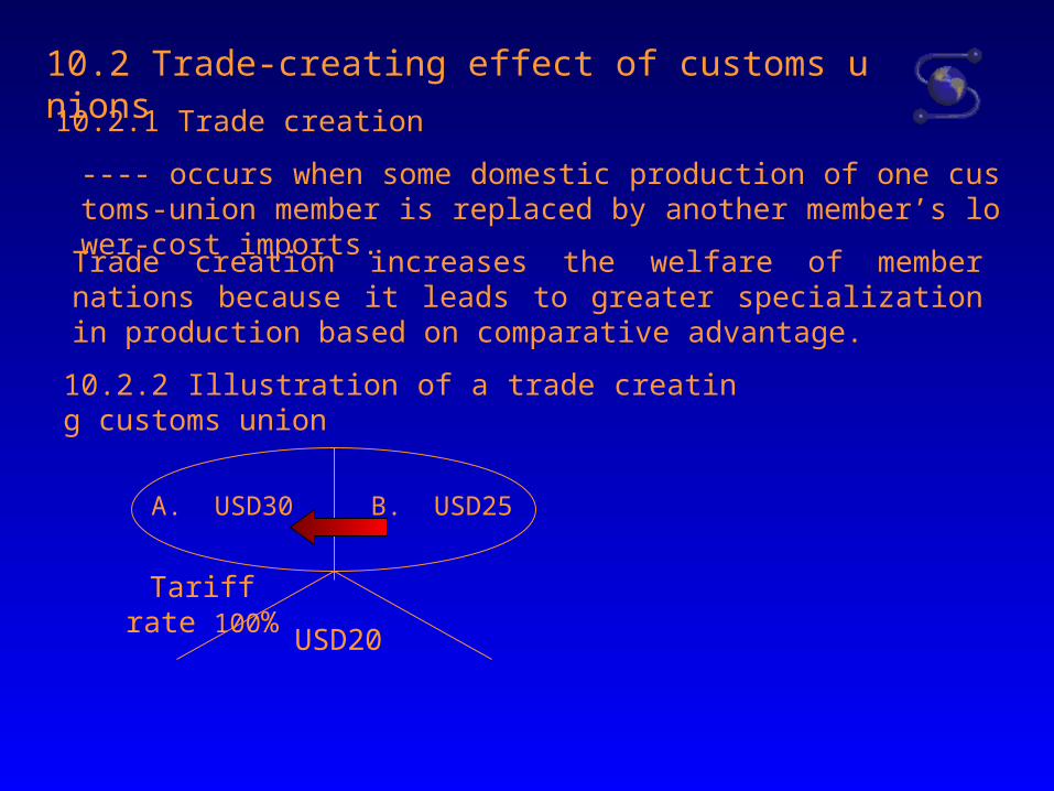
10.2 Trade-creating effect of customs unions

10.2.1 Trade creation

---- occurs when some domestic production of one customs-union member is replaced by another member’s lower-cost imports.

Trade creation increases the welfare of member nations because it leads to greater specialization in production based on comparative advantage.

10.2.2 Illustration of a trade creating customs union

A. USD30 B. USD25

USD20

Tariff rate 100%

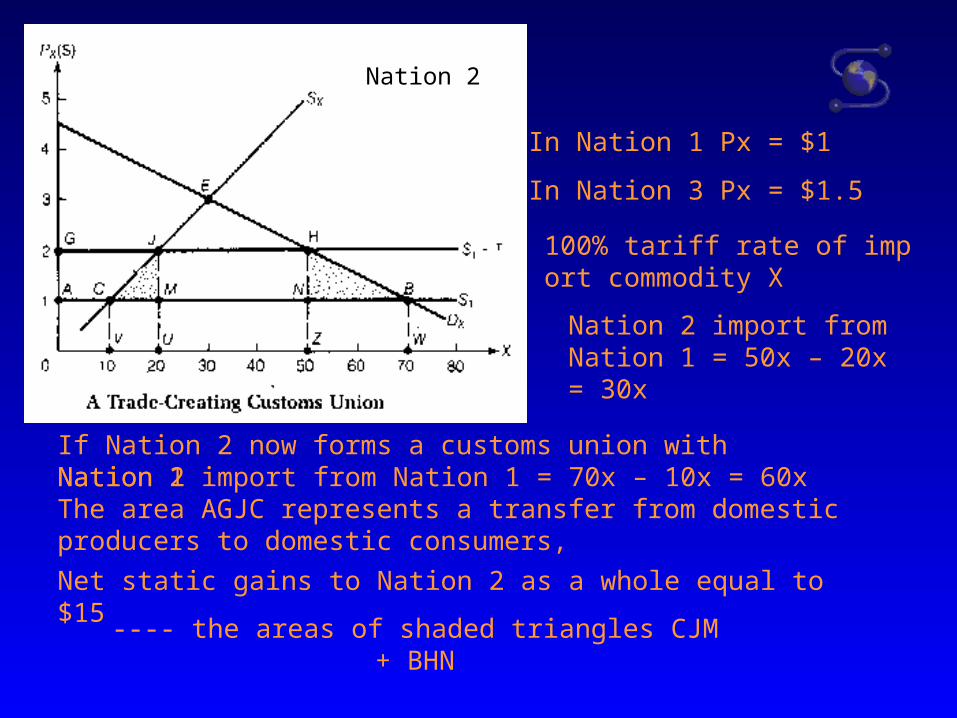
In Nation 1 Px = $1

In Nation 3 Px = $1.5

100% tariff rate of import commodity X

Nation 2

If Nation 2 now forms a customs union with Nation 1

Nation 2 import from Nation 1 = 50x – 20x = 30x

Nation 2 import from Nation 1 = 70x – 10x = 60xThe area AGJC represents a transfer from domestic producers to domestic consumers,

Net static gains to Nation 2 as a whole equal to $15

---- the areas of shaded triangles CJM + BHN

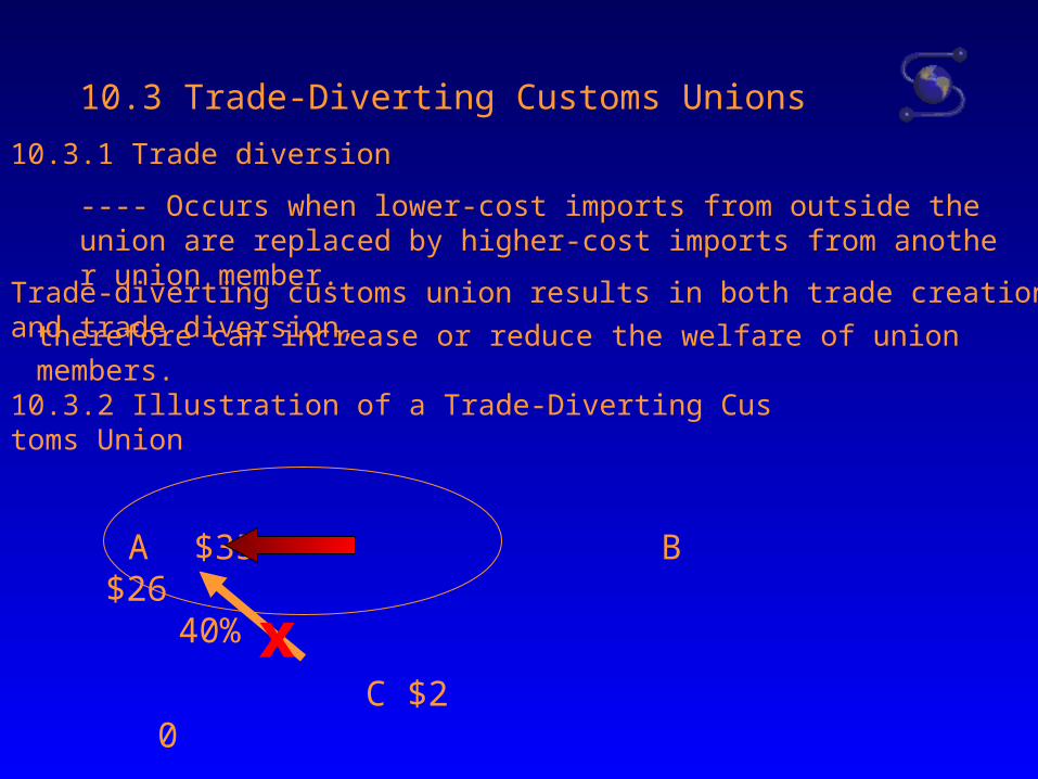
10.3 Trade-Diverting Customs Unions

10.3.1 Trade diversion

---- Occurs when lower-cost imports from outside the union are replaced by higher-cost imports from another union member.

Trade-diverting customs union results in both trade creation and trade diversion,

therefore can increase or reduce the welfare of union members.

10.3.2 Illustration of a Trade-Diverting Customs Union

A $35 B $26

40%

C $20

x

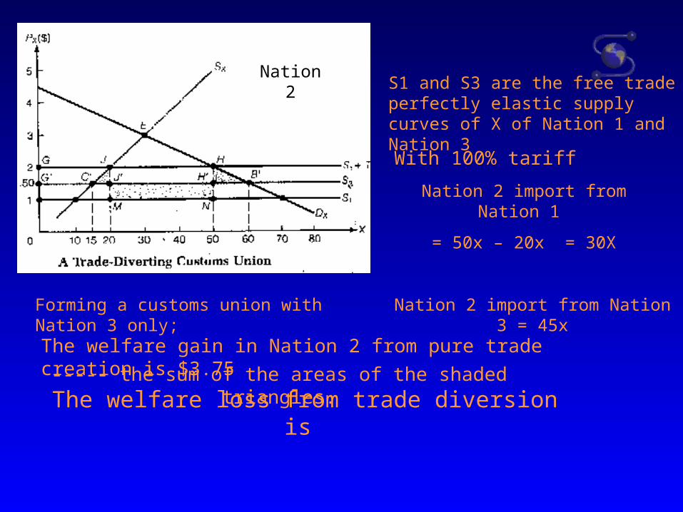
Nation 2S1 and S3 are the free trade perfectly elastic supply curves of X of Nation 1 and Nation 3

With 100% tariff

Nation 2 import from Nation 1

= 50x – 20x = 30X

Forming a customs union with Nation 3 only; Nation 2 import from Nation 3 = 45x

The welfare gain in Nation 2 from pure trade creation is $3.75

----- the sum of the areas of the shaded triangles.

The welfare loss from trade diversion is

10.4 Dynamic benefits from customs unions

10.4.1 Increased competition.

10.4.2 Economies of scale

10.4.3 Stimulus to investment.

10.4.4 Better utilization of the economic resources

of the entire community.