International Remittances and Financial Inclusion in … Research Working Paper 6991 International...
34
Policy Research Working Paper 6991 International Remittances and Financial Inclusion in Sub-Saharan Africa Gemechu Ayana Aga Maria Soledad Martinez Peria Development Research Group Finance and Private Sector Development Team July 2014 WPS6991 Public Disclosure Authorized Public Disclosure Authorized Public Disclosure Authorized Public Disclosure Authorized Public Disclosure Authorized Public Disclosure Authorized Public Disclosure Authorized Public Disclosure Authorized
Transcript of International Remittances and Financial Inclusion in … Research Working Paper 6991 International...

Policy Research Working Paper 6991
International Remittances and Financial Inclusion in Sub-Saharan Africa
Gemechu Ayana Aga Maria Soledad Martinez Peria
Development Research GroupFinance and Private Sector Development TeamJuly 2014
WPS6991P
ublic
Dis
clos
ure
Aut
horiz
edP
ublic
Dis
clos
ure
Aut
horiz
edP
ublic
Dis
clos
ure
Aut
horiz
edP
ublic
Dis
clos
ure
Aut
horiz
edP
ublic
Dis
clos
ure
Aut
horiz
edP
ublic
Dis
clos
ure
Aut
horiz
edP
ublic
Dis
clos
ure
Aut
horiz
edP
ublic
Dis
clos
ure
Aut
horiz
ed

Produced by the Research Support Team
Abstract
The Policy Research Working Paper Series disseminates the findings of work in progress to encourage the exchange of ideas about development issues. An objective of the series is to get the findings out quickly, even if the presentations are less than fully polished. The papers carry the names of the authors and should be cited accordingly. The findings, interpretations, and conclusions expressed in this paper are entirely those of the authors. They do not necessarily represent the views of the International Bank for Reconstruction and Development/World Bank and its affiliated organizations, or those of the Executive Directors of the World Bank or the governments they represent.
Policy Research Working Paper 6991
This paper is a product of the Finance and Private Sector Development Team, Development Research Group. It is part of a larger effort by the World Bank to provide open access to its research and make a contribution to development policy discussions around the world. Policy Research Working Papers are also posted on the Web at http://econ.worldbank.org. The authors may be contacted at [email protected] and [email protected].
This paper uses World Bank survey data, including about 10,000 households in five countries—Burkina Faso, Kenya, Nigeria, Senegal, and Uganda—to investigate the link between international remittances and households’ financial inclu-sion in Sub-Saharan Africa. The paper finds that receiving
international remittances increases the probability that the household opens a bank account in all the five countries. This result is robust to controlling for the potential endoge-neity of remittances, using as instruments indicators of the migrants’ economic conditions in the destination countries.

International Remittances and Financial Inclusion in Sub-Saharan Africa
Gemechu Ayana Aga and Maria Soledad Martinez Peria∗
JEL classification: F37, G21, 016
Keywords: remittances, financial inclusion
∗Gemechu Ayana Aga is a Private Sector Development Analyst in the Enterprise Analysis unit of the World Bank. Maria Soledad Martinez Peria is a Research Manager in the Development Research Group of the World Bank. We are grateful to Sonia Plaza for help in understanding the data. The opinions expressed in this paper are our own and do not represent the views of the World Bank, its Executive Directors or the countries they represent. Corresponding author: Maria Soledad Martinez Peria. 1818 H St., N.W., Washington D.C., 20433. (202) 458-7341.
1

I. Introduction
Remittances to Sub-Saharan Africa (SSA) have increased steadily in recent decades and
are estimated to have reached about $32 billion in 2013.1 Although smaller than the official
development assistance and foreign direct investment inflows, remittances constitute important
resource inflows to the region. In 2012 remittances accounted for about 4 percent of the GDP of
a typical country in Sub-Saharan Africa with consistent data on official remittances inflows, and
accounted for over 5 percent of the GDP in about ten of the countries in the region. The
magnitude is sizeable even in some of the larger countries. For instance, recorded remittances to
Nigeria amounted to about 8 percent of GDP in 2012, the corresponding figure being about 10
percent for Senegal. The importance of remittances is particularly evident in some of the smaller
countries of the region. In Lesotho and Liberia, for instance, remittances account for over 20
percent of the GDP. The true size of remittances is believed to be substantially higher given that
officially reported figures ignore remittances transferred through informal channels.
Though studies have shown that remittances can affect aggregate financial development
in SSA - as measured by the share of deposits or M2 to GDP (Gupta et al. 2009), to our
knowledge there is no evidence for this region on the impact of remittances on household
financial inclusion defined as the use of financial services.2 This question is important because
there is growing evidence that financial inclusion can have significant beneficial effects for
households and individuals. In particular, the literature has found that providing individuals
access to savings instruments increases savings (Aportela, 1999, Ashraf et al., 2014), female
1 All country-level aggregate remittance inflows data are from the World Bank. See Eigen-Zucchi et al. (2013) for the latest data. 2 There is a vast literature examining the impact of remittance on various outcome measures, such as poverty (Acosta et al., 2007; Yang 2008; Anyanwu and Erhijakpor, 2010), health (Lu, forthcoming; De and Ratha, 2012), education (Yang, 2008; Edwards and Ureta, 2003), labor supply (Rodriguez and Tiongson, 2001; Kim, 2007), entrepreneurship (Yang, 2008; Amuedo-Dorantes and Pozo, 2006b), etc. Adams (2011) provides a review of some of the key literature on the household level impact of remittances.

empowerment (Ashraf et al., 2010), productive investment (Dupas and Robinson, 2009), and
consumption (Dupas and Robinson, 2009 and Ashraf, et al., 2010).3 Furthermore, the topic of
financial inclusion has gained importance among international bodies, such as the UN and the
Group of Twenty (G-20). In May 2013, the UN High-Level Panel presented the
recommendations for post-2015 UN Development Goals, which included universal access to
financial services as a critical enabler for job creation and equitable growth. In September 2013,
the G20 reaffirmed its commitment to financial inclusion as part of its development agenda.4
This paper explores the link between international remittances and one aspect of financial
inclusion in SSA: households’ use of bank accounts. This issue is particularly important for SSA,
given that on average only 24 percent of the population has an account with a formal financial
institution. In contrast, 55 percent of adults in East Asia, 35 percent in Eastern Europe, 39
percent in Latin America, and 33 percent in South Asia have accounts.
Remittances may affect households’ use of bank accounts in at least two ways. First,
remittances might increase the demand for savings instruments. The fixed costs of sending
remittances make the flows lumpy, potentially providing households with excess cash for some
period of time. This might increase their demands for deposit accounts, since financial
institutions offer households a safe place to store this temporary excess cash. Second,
remittances recipients’ exposure to banks, for example, when banks act as remittances paying
agents, may familiarize them with the services offered by banks and increase their demand for
bank accounts. Therefore, so long as lack of awareness is the main reason for households’
financial exclusion, remittances may increase households’ use of bank accounts.
3 There is also evidence that access to credit and to insurance products has beneficial effects but the results are not as strong or robust (Karlan and Murdoch, 2009 and Roodman, 2012). 4 See the G20 Leader’s Declaration from the St. Peterburg Summit at: http://en.g20russia.ru/news/20130906/782776427.html
3

Using World Bank survey data including about 10,000 households in five countries --
Burkina Faso, Kenya, Nigeria, Senegal and Uganda – we find that receiving international
remittances increases the probability that the household opens a bank account in all the countries
in our study. This result is robust to controlling for the potential endogeneity of remittances,
using as instruments indicators of the migrants’ economic conditions in the destination countries.
Our paper is related to an emerging literature on remittances and financial inclusion.
Using household level data from El Salvador, Anzoategui et al. (2014) show that remittances
have a positive effect on the likelihood that households have a bank account. Relatedly, Ashraf et
al. (forthcoming) find that migrants from El Salvador save more in the home country when
offered accounts providing greater ability to monitor and control savings. On the other hand,
Brown et al. (forthcoming) provide household level evidence that remittances have a negative,
and at best no, effect on the propensity of having a bank account in Azerbaijan, while finding a
positive and significant, but very small size, effect in Kyrgyzstan.
The rest of the paper is organized as follows. Section II discusses the data used and the
empirical methodology implemented. Section III presents the results, while section IV concludes.
II. Data and Methodology
Data used in the paper come from household surveys conducted by the World Bank in
2010 in six Sub-Saharan African countries: Burkina Faso, Kenya, Nigeria, Senegal, South
Africa, and Uganda. We use survey data for the first five countries since South Africa is regarded
as a remittances sending country.
4
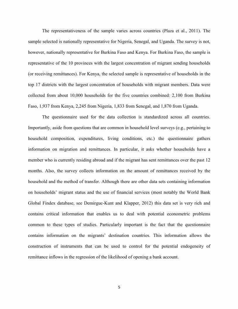
The representativeness of the sample varies across countries (Plaza et al., 2011). The
sample selected is nationally representative for Nigeria, Senegal, and Uganda. The survey is not,
however, nationally representative for Burkina Faso and Kenya. For Burkina Faso, the sample is
representative of the 10 provinces with the largest concentration of migrant sending households
(or receiving remittances). For Kenya, the selected sample is representative of households in the
top 17 districts with the largest concentration of households with migrant members. Data were
collected from about 10,000 households for the five countries combined: 2,100 from Burkina
Faso, 1,937 from Kenya, 2,245 from Nigeria, 1,833 from Senegal, and 1,870 from Uganda.
The questionnaire used for the data collection is standardized across all countries.
Importantly, aside from questions that are common in household level surveys (e.g., pertaining to
household composition, expenditures, living conditions, etc.) the questionnaire gathers
information on migration and remittances. In particular, it asks whether households have a
member who is currently residing abroad and if the migrant has sent remittances over the past 12
months. Also, the survey collects information on the amount of remittances received by the
household and the method of transfer. Although there are other data sets containing information
on households’ migrant status and the use of financial services (most notably the World Bank
Global Findex database, see Demirguc-Kunt and Klapper, 2012) this data set is very rich and
contains critical information that enables us to deal with potential econometric problems
common to these types of studies. Particularly important is the fact that the questionnaire
contains information on the migrants’ destination countries. This information allows the
construction of instruments that can be used to control for the potential endogeneity of
remittance inflows in the regression of the likelihood of opening a bank account.
5

In Burkina Faso, Kenya, and Senegal, over 20 percent of the households report receiving
remittances from members residing in other countries. This contrasts with Nigeria and Uganda
where less than 6 percent of households report receiving international remittances.
Furthermore, the survey includes questions on households’ access to and use of formal
financial services. In particular, households are asked whether any member of the household has
a bank account. For households that have a member residing abroad, there is also a question
asking if the household opened a bank account after the migrant left.
There is significant variation across countries in terms of households’ financial inclusion.
Over 60 percent of the households sampled from Kenya report that at least a member of the
household has a bank account. In Burkina Faso, only 11 percent of households sampled report
having a bank account. About 44 percent of households in Nigeria report having at least a
member with a bank account. The corresponding figure is 23 percent for Uganda and 20 percent
for Senegal.5
A relatively smaller proportion of the households with an international migrant note that
a member of the household opened a bank account after the international migrant left the
household. Higher values are reported in Kenya (and Uganda) where about 18 (and 8) percent of
the households noted opening such account after the international migrant left the family. For the
rest of the countries it is less than 5 percent.
We analyze the link between remittances and financial inclusion by estimating the
following model:
5A nationally representative survey of household financial inclusion indicates slightly lower figures for all the countries, except for Burkina Faso (Demirguc-Kunt and Klapper, 2012). The survey indicates that only about 6 percent of the population in Senegal has an account in formal financial institutions. Similarly, just about 42 percent of households in Kenya have an account in formal financial institutions. The corresponding figures for Uganda and Nigeria are 20 and 30 percent, respectively. In Burkina Faso, about 13 percent of the households report to have such account.
6

FIh = α + β1 ∗ IntRemh + β2 ∗ Xh + εh (1)
Where h is the household, FI is the measure of financial inclusion, IntRem is the measure
of households’ remittances recipient status, X is a matrix of other household level variables, and
ε is the error term. We use two measures of financial inclusion. A dummy variable that takes a
value of 1 if any member of the household has a bank account, and zero otherwise. We also use a
dummy that takes a value of 1 if the household opened a bank account after the migrant left the
household, and zero otherwise. Note that this variable is only defined for the subset of
households that have a migrant residing overseas.
We also use two measures of households’ remittances recipient status. The first measure
is a dummy indicating if the household received remittances from a migrant residing abroad. The
second measure is the actual amount of remittances received by the household over the 12
months prior to the survey year.
We also control for additional variables that may affect households’ financial inclusion
(see Allen, Demirguc-Kunt, Klapper and Martinez Peria, 2012). We control for the household’s
education by including the proportion of adults in the household with at least a high school
diploma. To capture the effect of household wealth on the demand and usage of financial
services, we use the household’s per capita expenditure. We also include the average age of the
household members to account for a potential effect of age on financial inclusion. Given the role
of proximity to financial services in access to finance and considering that financial services are
mainly concentrated in urban areas, we include an urban dummy taking a value of 1 if the
household resides in an urban area and zero otherwise. Table 1 lists all the variables used in our
empirical analysis and provides definitions. We report summary statistics for all the variables
used in Table 2.
7

III. Results and Discussion
Baseline Regression
Table 3 provides the estimates of the baseline regression, where the dependent variable is
the dummy that equals one for households that have bank accounts. We employ a simple Linear
Probability model (LPM)6 to estimate the regression equation, and standard errors are clustered
at the region7 and region fixed effects are controlled for. The results show that international
remittances have a positive and significant effect in all of the five countries. The size of the point
estimate varies across countries. For instance, in Kenya and Nigeria, receiving international
remittances increases the probability of a household having a bank account by about 10
percentage points. The size of the coefficient is larger for Uganda, where receiving international
remittances increases the probability of having a bank account by about 15 percentage points.
The size of the coefficient is smaller for Senegal and Burkina Faso, where receiving international
remittances increases the likelihood of having a bank account by about 5 and 6 percentage
points, respectively.
As predicted, education enters with a positive and significant coefficient for all the
countries. Average age enters with a negative and significant coefficient for two of the five
countries, indicating that the older the household members are, the lower the likelihood that
households will have a bank account. For Nigeria, however, the variable enters with a positive
and significant effect, indicating the likelihood of having a bank account increases with age. The
6 Though our dependent variable is a limited dependent variable, we conduct our estimations with a linear probability model for a number of reasons. First, coefficients from this model can be easily interpreted. Second, fixed effect estimations are consistent. On the other hand, in the presence of fixed effects, probit models suffer from the incidental parameters problem which leads to inconsistent estimates. 7 Since the geographic units vary across countries, we define region as the largest geographic unit in the sample for each country. In the case of Burkina Faso, region refers to administrative regions and for Nigeria it refers to states. For Kenya and Uganda, regions refer to the administrative districts, while for Senegal, the regional classification is based on the administrative provinces.
8
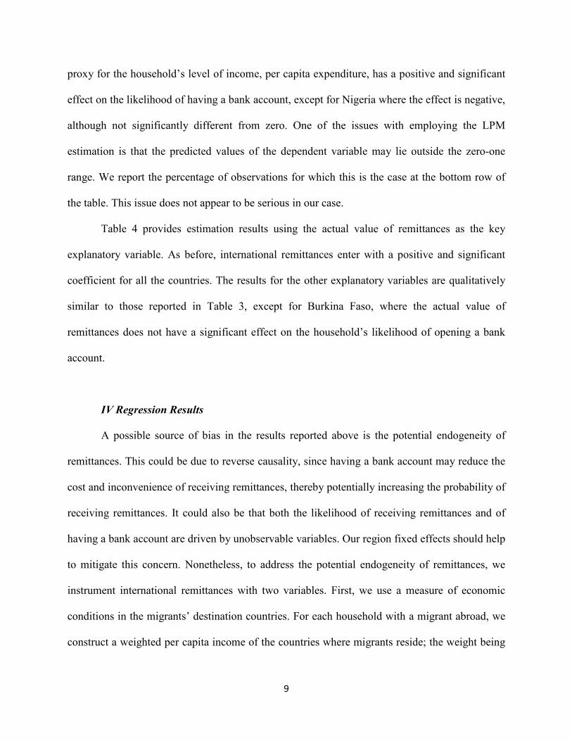
proxy for the household’s level of income, per capita expenditure, has a positive and significant
effect on the likelihood of having a bank account, except for Nigeria where the effect is negative,
although not significantly different from zero. One of the issues with employing the LPM
estimation is that the predicted values of the dependent variable may lie outside the zero-one
range. We report the percentage of observations for which this is the case at the bottom row of
the table. This issue does not appear to be serious in our case.
Table 4 provides estimation results using the actual value of remittances as the key
explanatory variable. As before, international remittances enter with a positive and significant
coefficient for all the countries. The results for the other explanatory variables are qualitatively
similar to those reported in Table 3, except for Burkina Faso, where the actual value of
remittances does not have a significant effect on the household’s likelihood of opening a bank
account.
IV Regression Results
A possible source of bias in the results reported above is the potential endogeneity of
remittances. This could be due to reverse causality, since having a bank account may reduce the
cost and inconvenience of receiving remittances, thereby potentially increasing the probability of
receiving remittances. It could also be that both the likelihood of receiving remittances and of
having a bank account are driven by unobservable variables. Our region fixed effects should help
to mitigate this concern. Nonetheless, to address the potential endogeneity of remittances, we
instrument international remittances with two variables. First, we use a measure of economic
conditions in the migrants’ destination countries. For each household with a migrant abroad, we
construct a weighted per capita income of the countries where migrants reside; the weight being
9

the share of household members that reside in each destination country. Instrumenting
remittances using economic conditions in the migrants’ destination countries is a similar
procedure followed in other studies (Anzoategui et al., 2011; Aggarwal et al., 2011). Second, we
use a measure of the employment status of the migrant member of the household residing abroad.
For each household, we construct a measure taking the proportion of international migrants from
the household that are currently employed. We expect the two variables to positively affect the
propensity to remit and the size of remittances sent by migrants. For instance, migrants living in
high income countries are, all else equal, more likely to send remittances. Similarly, the larger
the proportion of migrants employed, the more likely they are to send remittances.
Table 5 provides estimation results of the first stage regressions, instrumenting the
dummy for international remittances with the two variables described above. For each country,
column (1) shows the first stage regression results using the weighted per capita income as
instrument, column (2) presents the results using employment status of the migrant as
instrument, while column (3) displays the results using both instruments. As can be seen, for all
the countries in our analysis, the instruments enter with the expected sign and are statistically
significant, both when entering the equation individually as well as jointly.
The bottom rows of the table provide some diagnostic tests for the validity of the
instruments. We report the Kleibergen-Paap Lagrange Multiplier (LM) statistic to test the
relevance of the instrument, i.e., the extent to which the two instruments are correlated with
international remittances. Under the null hypothesis that the instruments are not relevant, this
statistic follows a chi-squared distribution. In our case, the null hypothesis is rejected for all the
countries, indicating that the instruments are relevant. We also report the Kleibergen-Paap
transformed F statistic to test for the weak instruments problem. The test statistics rejects the null
10

of weak instruments using the critical values reported in Stock and Yogo (2005).8 In addition,
the variables are also found to be orthogonal to the error process of financial inclusion on the
basis of the Hansen J statistic for over-identifying restrictions (column (3) for each of the
countries). Thus, the instrument set is deemed valid for the purpose of the current exercise.
Finally, given these findings, we can test for whether international remittances is an endogenous
variable in the first place. This is essentially a postmortem type of test to see if we needed to
instrument for international remittances in the first place. The test is based on C-statistic and
follows a chi-squared distribution under the null hypothesis that the endogenous regressor can be
treated as exogenous and, therefore, no need for instrumenting in the first place. In almost all the
cases, except marginally so for Senegal, the test does not reject the null hypothesis of exogeneity
of the international remittances variable. This means that endogeneity is not a serious issue in the
first place and the baseline regression results are generally valid.
Table 6 presents the estimation results of the second stage regressions. For each country,
column (1) provides estimation results, using the weighted per capita income of the migrant
destination as the instrument; column (2) shows results of the regressions using employment
status of the international migrant as instrument, while column (3) provides the results using the
two instruments jointly. In all the regressions, standard errors are clustered at the regional level
and regional fixed effects are controlled for. As can be seen, for Kenya, international remittances
enters with positive and significant coefficient in the three specifications. Interestingly, the size
of the coefficient is essentially similar to the baseline regressions. The results for the other
control variables are also identical to the estimates in the baseline regression. For Uganda as
8 The critical value for the 10% (15%) maximal IV size is 16.38 for one instrument. When remittances is instrumented by the two instruments, the corresponding values are 19.93(11.56). The test statistics reported in the table are higher than the critical values of the 10% maximal IV size, except in the first column for Senegal, which is significant at 15%, indicating that the instruments used are not weak enough to distort the results of the IV regression.
11

well, international remittances enters with a positive and significant coefficient, and the size of
the coefficient is slightly higher than the estimates in the baseline regression. Similarly, the
estimates of the control variables are broadly comparable to the respective values reported in the
baseline regression. For Burkina Faso, however, the international remittances variable is
significant marginally and only in one of the three specifications, i.e., when the two instruments
are used jointly. Remittances ceases to be significant when the two instruments enter separately.
For Senegal, once again, the international remittances variable has a significant effect on
households’ financial inclusion, and the size of the coefficient is almost twice that of the baseline
regression.
We also report similar results for the actual value of international remittances. Table 7
contains the results of the first stage regressions using the actual value of remittances. The
instruments enter with the expected sign and are statistically significant, both when used
individually as well as jointly. The diagnostic tests indicate that the instruments do not suffer
from the weak instruments problem and that they are valid instruments. The diagnostic tests also
indicate that the international remittances variable is not endogenous in the regression and,
hence, the baseline regression results reported in Table 4 are valid. Table 8 presents the
estimation results for the second stage regressions. The results are qualitatively similar to what is
reported in Table 4.
We report two sets of additional results meant to check for the robustness of our findings.
First, we re-estimate results reported in Table 5 to 8 by using weighted regression for countries
where relevant weighting information is available. Second, we report regression results using a
dummy for whether the household opened a bank account after international migrant left the
household. We will discuss each of them in turn.
12

Since the survey is based on a non-random sampling technique, sampling weights are
provided for all the countries except for Kenya. Although there are compelling reasons to use
sampling weights when estimating population descriptive statistics based on a non-random
sample data, the case for using sampling weights in analysis dealing with causal inferences is a
bit nuanced (Deaton 1997; Haider et al 2013; Winship and Radbill 1994). Haider et al., (2013)
provide three potential motives for using sampling weights in such analysis.9 A textbook case is
where one suspects the error term to be heteroskedastic, arising from the error term varying with
the criteria used in the sampling design. Properly weighted regressions can reduce the problem of
heteroskedasticity and could potentially improve the efficiency of the estimates. However, using
sampling weights in an otherwise homoscedastic error term produces an inefficient estimate. The
second case is when the sampling design is endogenous, i.e., when the sampling criteria is a
function of the dependent variable modeled in the regression analysis. In such cases, unweighted
OLS produces biased and inconsistent estimates since certain group could be over/under
represented in the sample relative to the population, necessitating the need to correct for this by
applying proper sampling weights. On the contrary, if the sampling design is exogenous, using
sampling weights may make the estimates inefficient. The third scenario where one needs to use
sampling weights in regression analysis for causal inference is when there is heterogeneity in the
impact of explanatory variables that is somehow a function of the sampling criteria used. In our
context, the sampling criterion is based on the migrant status of the households and clearly not a
function of the dependent variable modeled. Hence, the second case for the need to use sampling
weights does not apply to our case. The potential heteroskedasticity arising from some form of
misspecifications is, however, already taken care of since we report robust standard errors,
9 Haider et al. (2013) also provide a comprehensive discussion of the trade-offs involved in using sampling weights in regression analysis.
13

corrected for unknown heteroskedasticity. Nevertheless, we report the results of the weighted IV
regression for completeness.10
Appendix Tables 1 to 4 presents the first and second stage IV weighted regressions using
the dummy and actual value of remittances. Appendix Table 1 provides the first stage IV
regression results by instrumenting the remittances dummy using the two instrumental variables
noted earlier. The estimation results are broadly comparable to the results based on unweighted
regressions reported in Tables 5. In particular, the estimated coefficients of the two instrumental
variables remain virtually unchanged by using sampling weights. Appendix Table 2 presents the
second stage regression results of the IV estimation using a dummy for remittances. For Uganda
and to some extent for Senegal, the results of the weighted and unweighted estimations are
broadly similar. However, our key variable is no longer significant for Burkina Faso in all three
specifications and for Nigeria in two of the three specifications. Weighted regression
substantially reduces the size of the estimated coefficients for Nigeria, while it increased the
standard error for Burkina Faso. Appendix Table 3 and Table 4 report respective results for
weighted regression estimates using the actual value (in US$) of remittances received by the
household.
We also report regression results using a dummy for whether the household has opened a
bank account after international migrant left the household in Appendix Table 5 and 6. We
estimate results with this alternative indicator of the use of bank accounts because we believe
this variable is less likely to be affected by reverse causality issues given the nature of the
questions (i.e., the fact that it assumes that the migration occurred first). Although a relatively
10 We also report the estimate for Kenya, although there are no sampling weights in the survey for the country.
14

small fraction of the households report opening such account11, the results are positive and
significant for all the countries (except for Uganda in some of the estimations), indicating that
international remittances increases the probability that the household opens a bank account after
the migrant left.
IV. Conclusion
Remittances inflows to SSA have been increasing over recent years, growing on average
at about 4 percent between 2010 and 2013. The region is estimated to have received about $32
billion US$ in 2013. In addition to serving as a lifeline for many households, remittances inflows
can impact the aggregate level of financial development and households’ use of formal financial
services. Although there are studies examining the impact of remittances on aggregate financial
sector development in SSA, to our knowledge, there are no studies on the impact of remittances
on households’ financial inclusion.
Using survey data for approximately 10,000 households in five countries in SSA, we
show that international remittances play an important role in enhancing households’ financial
inclusion. The findings of the paper add to the nascent literature on remittances and financial
inclusion at the household level.
11 Note that the variable “bank account after international migrant left” is constructed only for households that have international migrants. Therefore, the regression results reported in Appendix tables 5 and 6 are based on sub-set of sample used in the rest of the tables.
15
References
Acosta, P., Fajnzylber, P., and Lopez, H. (2007). The Impact of Remittances on Poverty and Human Capital: Evidence from Latin American Household Surveys. World Bank Policy Research Working Paper 4247. Adams, R. (2011). Evaluating the Economic Impact of International Remittances on Developing Countries Using Household Surveys: A Literature Review. Journal of Development Studies, vol. 47, Issue 6, pp 809-828. Aggarwal, R., Demirguc-Kunt, A., and Martinez Peria, M. S. (2011). Do Remittances Promote Financial Development? Journal of Development Economics, vol. 96, pp 255-264. Allen, F., Demirgüç-Kunt, A., Klapper, L., and Martínez Pería, M.S. (2012). The Foundations of Financial Inclusion: Understanding Ownership and Use of Formal Accounts. World Bank Policy Research Working Paper 6290. Amuedo-Dorantes, C. and Pozo, S. (2006a). Migration, Remittances and Male and Female Employment Patterns. American Economic Review, 96(2), pp. 222–226. Amuedo-Dorantes, C,. and Pozo, S. (2006b). Remittance Receipt and Business Ownership in the Dominican Republic. The World Economy, vol. 29, Issue 7, pp 939-956. Anyanwu, J. and Erhijakpor, A. (2010). Do International Remittances Affect Poverty in Africa? African Development Review, vol. 22, No. 1, 51-91. Anzoategui, D., Demirgüç-Kunt, A., and Martínez Pería, M.S. (2014). Remittances and Financial Inclusion: Evidence from El Salvador. World Development 54, 338-349, 2014 Aportela, F., (1999). Effects of Financial Access on Savings by Low-Income People. MIT Department of Economics Dissertation Chapter 1. Ashraf, N., Aycinena, D., Martinez, C. and Yang., D. (forthcoming) Savings in Transnational Households: A Field Experiment among Migrants from El Salvador. Review of Economics and Statistics.
Ashraf, N., Karlan, D., and Yin,W., (2010). Female Empowerment: Further Evidence from a Commitment Savings Product in the Philippines. World Development 28, 333-344. Brown, R., Carmignani, F., and Fayad, G. (Forthcoming). Migrant’s Remittance and Financial Development: Macro and Micro-level Evidence of a perverse relationship, The World Economy. De, P. and Ratha, D. (2012). Impact of Remittances on Household Income, Asset and Human Capital: Evidence from Sri Lanka. Migration and Development, vol. 1, no 1, pp.163-179.
16

Deaton, A. (1997). The Analysis of Household Surveys: A Microeconometric Approach to Development Policy. Johns Hopkins University Press, Baltimore, MD. Demirguc-Kunt, A., Lopez Cordova, E., Martinez Peria, M.S., and Woodruff, C. (2011). Remittances and Banking Sector Depth: Evidence from Mexico, Journal of Development Economics, vol. 95, 229-241. Demirguc-Kunt, A. and Klapper, L. (2012). Measuring Financial Inclusion: The Global Findex Database, World Bank Policy Research Paper 6052. Dupas, P., and Robinson, J., (2009). Savings Constraints and Microenterprise Development: Evidence from a Field Experiment in Kenya. National Bureau of Economic Research Working Paper 14693. Edwards, A.C., and Ureta, M., (2003). International Migration, Remittances, and Schooling: evidence from El Salvador, Journal of Development Economics, vol. 72, Issue 2, pp.429-461. Eigen-Zucchi, C., Plaza, S., Ratha, D., Wyss, H,, and Yi, H. (2013). Migration and Remittance Flows: Recent Trends and Outlook 2013-2016, Migration and Development Brief 21,The World Bank. Gupta, S., Pattillo, C., and Wagh, S., (2009). Impact of Remittances on Poverty and Financial Development in Sub-Saharan Africa. World Development vol. 37, no. 1 pp104-115. Haider, S., Solon, G., and Wooldridge, G. (2013). What Are We waiting for?, NBER Working Paper 18859. Karlan, D., and Morduch, J., (2009) “Access to Finance”, In Dani Rodrik and Mark Rosenzweig, eds., Handbook of Development Economics, Volume 5. Amsterdam: Elsevier. Pages 4704 - 4784. Kim, N. (2007). The Impact of Remittances on Labor Supply: The Case of Jamaica, World Bank Policy Research Working Paper 4120. Lu, Y. (Forthcoming). Household Migration, Remittances and Their Impact on Health in Indonesia, International Migration. Plaza, S., Navarrete, M., and Ratha, D. (2011). Migration and Remittances Household Survey in Sub-Saharan Africa: Methodological Aspect and Main findings, Mimeo, Development Prospects Group, The World Bank, Washington, D.C. Rodriguez, E. and Tiongson, E. (2001). Temporary Migration Overseas and Household Labor Supply: Evidence from Urban Philippines. International Migration Review, vol. 35, Issue 3, pp. 709-725.
17

Roodman, D. (2012). Due Dilligence: An Impertinent Inquiry into Microfinance. Center for Global Development. Washington, D.C. Stock, J., and Yogo, M. (2005). Testing for Weak Instruments in Linear IV Regression. Ch. 5 in J.H. Stock and D.W.K. Andrews (eds), Identification and Inference for Econometric Models: Essays in Honor of Thomas J. Rothenberg, Cambridge University Press. Yang, D. (2008). International Migration, Remittances and Household Investment: Evidence from Philippine Migrants’ Exchange Rate Shocks, The Economic Journal, vol. 118, pp. 591-630. Winship, C. and Radbill, L. (1994). Sampling Weights and Regression Analysis. Sociological Methods and Research, vol. 23 no.2 pp. 230–257.
18

Table 1: Definition of variables
Variables Definitions
Bank account A dummy variable taking a value of one if the household has a bank
account, and zero otherwise.
Bank account after international migrant left A dummy variable taking a value of one if the household has opened a bank account after the member left the households to go abroad, and zero otherwise. This variable is defined only for households with at least one of their members residing abroad.
International remittances A dummy variable taking a value of 1 if the household has received remittances from abroad over the past 12 months and zero otherwise.
ln(Actual value of remittances) The per capita value (in US$) of total remittances received from abroad by the household over the past 12 months.
High School The fraction of adult members of household with high school and above level of education.
Age
The average age of the members of the household.
ln(Per capita spending)
Household’s per capita annual expenditure.
Urban Dummy taking a value of one if the household resides in an urban area, and zero otherwise.
19

Table 2: Descriptive statistics Summary statistics of variables used in the analysis. Except for Kenya, in all other cases, all summary statistics are weighted by relevant sampling weights.
Variable Kenya Uganda Nigeria Burkina Faso Senegal Mean Sd. Mean Sd. Mean Sd. Mean Sd. Mean Sd. Bank Account 0.63 0.48 0.23 0.42 0.44 0.50 0.11 0.32 0.20 0.40 Bank after International Migrant left 0.18 0.39 0.08 0.27 0.14 0.35 0.01 0.10 0.04 0.20 International Remittances 0.24 0.43 0.05 0.22 0.06 0.23 0.20 0.40 0.24 0.43 ln(Actual Value of International remittances) 1.25 2.34 0.19 0.92 0.19 0.86 0.45 1.00 0.92 1.80 High School 0.48 0.41 0.19 0.33 0.38 0.40 0.10 0.19 0.18 0.28 Age 29.86 14.08 24.65 11.91 23.26 9.58 22.08 8.50 24.18 8.20 ln(Per capita spending) 5.64 1.32 4.65 1.21 6.52 1.21 4.21 0.83 5.12 0.88 Urban 0.49 0.50 0.18 0.38 0.44 0.50 0.07 0.26 0.49 0.50 N 1937 1937 1870 1870 2245 2245 2100 2100 1833 1833 N (Bank after International Migrant Left) 711 711 249 249 580 580 694 694 620 620
20

Table 3: Baseline regression results for the probability of having a bank account on the dummy for international remittances
The dependent variable is a dummy equal to one if the household has a bank account and zero otherwise. International remittances is a dummy taking a value of 1 if the household has received remittances over the past 12 months, and zero otherwise. Other variables are defined in Table 1. Standard errors are clustered at the regional level and region level fixed effects are controlled for. t-statistics are in parentheses. *,**,*** denote significance at 10, 5, and 1 percent, respectively. Variable Kenya Uganda Nigeria Burkina Faso Senegal International Remittance 0.088*** 0.155*** 0.096*** 0.049** 0.058**
(3.866) (3.252) (5.370) (2.825) (2.854)
High School 0.394*** 0.479*** 0.447*** 0.148*** 0.476***
(10.946) (9.915) (10.014) (4.126) (14.101)
Age 0.000 -0.001 0.003** -0.003** -0.002***
(0.110) (-1.610) (2.662) (-3.501) (-3.706)
ln(Per capita spending) 0.056*** 0.063*** -0.012 0.077*** 0.080***
(4.321) (4.606) (-0.831) (4.102) (3.336)
Urban 0.080** 0.145*** 0.040 0.145 0.077***
(2.379) (4.128) (1.190) (1.468) (3.703)
Constant 0.065 -0.165*** 0.330*** -0.192* -0.293**
(0.852) (-2.792) (3.279) (-2.438) (-2.484)
Observations 1,937 1,870 2,245 2,100 1,833 R-squared 0.322 0.383 0.452 0.111 0.308 Percentage of observations outside the 0-1 range 4.285 5.882 0.0445 6.810 3.819
21
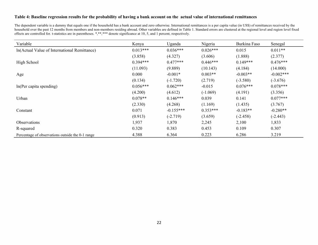
Table 4: Baseline regression results for the probability of having a bank account on the actual value of international remittances
The dependent variable is a dummy that equals one if the household has a bank account and zero otherwise. International remittances is a per capita value (in US$) of remittances received by the household over the past 12 months from members and non-members residing abroad. Other variables are defined in Table 1. Standard errors are clustered at the regional level and region level fixed effects are controlled for. t-statistics are in parentheses. *,**,*** denote significance at 10, 5, and 1 percent, respectively.
Variable Kenya Uganda Nigeria Burkina Faso Senegal ln(Actual Value of International Remittance) 0.013*** 0.036*** 0.026*** 0.015 0.011**
(3.858) (4.327) (3.606) (1.888) (2.377)
High School 0.394*** 0.477*** 0.446*** 0.149*** 0.476***
(11.093) (9.889) (10.143) (4.184) (14.000)
Age 0.000 -0.001* 0.003** -0.003** -0.002***
(0.134) (-1.720) (2.719) (-3.580) (-3.676)
ln(Per capita spending) 0.056*** 0.062*** -0.015 0.076*** 0.078***
(4.200) (4.612) (-1.069) (4.191) (3.356)
Urban 0.078** 0.146*** 0.039 0.141 0.077***
(2.330) (4.268) (1.169) (1.435) (3.767)
Constant 0.071 -0.155*** 0.353*** -0.183** -0.280**
(0.913) (-2.719) (3.659) (-2.458) (-2.443)
Observations 1,937 1,870 2,245 2,100 1,833 R-squared 0.320 0.383 0.453 0.109 0.307 Percentage of observations outside the 0-1 range 4.388 6.364 0.223 6.286 3.219
22

Table 5: First stage instrumental variable regressions for the remittances dummy
The dependent variable is a dummy equal to one if the household received international remittances over the past 12 months, and zero otherwise. The instruments are the weighted per capita income of the migrants’ destination countries and the proportion of migrants that are currently employed. Other variables are defined in Table 1. Standard errors are clustered at the regional level and region level fixed effects are controlled for. t-statistics are in parentheses. *,**,*** denote significance at 10, 5, and 1 percent, respectively
Kenya Uganda Nigeria Burkina Faso Senegal
(1) (2) (3) (1) (2) (3) (1) (2) (3) (1) (2) (3) (1) (2) (3)
High School -0.023 0.002 -0.012 0.058*** 0.053*** 0.048*** 0.016 0.017 0.009 0.015 0.046 0.045 -0.052 0.039 -0.006
(-1.109) (0.112) (-0.754) (3.319) (3.206) (3.041) (0.593) (0.691) (0.359) (0.349) (1.120) (1.118) (-1.564) (1.407) (-0.290)
Age -0.001 0.000 -0.001 -0.000 -0.000 -0.000 0.003*** 0.002** 0.001* 0.001 0.001 0.000 -0.003 -0.002 -0.002
(-0.892) (0.350) (-1.177) (-1.133) (-0.297) (-0.570) (3.357) (2.294) (2.035) (0.801) (0.921) (0.782) (-1.456) (-1.388) (-1.085)
ln (Per capita spending) 0.025* 0.026** 0.018* 0.019*** 0.014** 0.013** -0.006 0.003 0.002 -0.016 -0.008 -0.010 0.041*** 0.042*** 0.033***
(2.096) (2.725) (1.888) (3.096) (2.354) (2.428) (-0.581) (0.344) (0.240) (-1.138) (-1.069) (-1.154) (3.658) (3.834) (4.712)
Urban -0.050** -0.041** -0.037* 0.061** 0.043** 0.042** -0.022 -0.016 -0.018 -0.062** -0.000 -0.021 -0.050 -0.012 -0.029
(-2.413) (-2.143) (-2.064) (2.479) (2.373) (2.327) (-1.725) (-1.187) (-1.387) (-2.495) (-0.015) (-1.599) (-1.655) (-0.672) (-1.284)
Weighted per capita income in migrants’ destination countries 0.017***
0.008*** 0.002***
0.000** 0.002***
0.001*** 0.003**
0.001* 0.003***
0.002***
(15.481)
(6.851) (6.897)
(2.562) (17.536)
(4.484) (2.852)
(2.328) (8.129)
(8.524)
Proportion of migrants abroad currently employed 0.734*** 0.596*** 0.513*** 0.480*** 0.733*** 0.571*** 0.601*** 0.589***
0.718*** 0.531***
(20.283) (13.129) (13.895) (12.927) (12.881) (7.282) (14.272) (14.361)
(23.203) (18.101)
N 1937 1937 1937 1870 1870 1870 2245 2245 2245 2100 2100 2100 1833 1833 1833
Kleibergen-Paap LM Statistic 14.214 15.160 15.239 6.569 10.661 13.551 9.964 9.999 10.117 5.809 4.462 6.064 5.591 6.888 7.258
P-value 0.000 0.000 0.000 0.010 0.001 0.001 0.002 0.002 0.006 0.016 0.035 0.048 0.018 0.009 0.027
Kleibergen-Paap F-Statistic 239.651 411.389 177.783 47.566 193.084 86.374 307.496 165.927 242.603 8.134 203.680 108.088 66.088 538.370 164.752
Hansen J-statistic 0.000 0.000 0.260 0.000 0.000 2.553 0.000 0.000 2.720 0.000 0.000 1.236 0.000 0.000 0.804
P-value
0.610
0.110
0.099
0.266
0.370
Endogeneity test 0.085 0.129 0.045 2.592 2.197 0.300 2.673 0.237 0.402 1.122 0.589 0.372 2.760 2.797 2.563
P-value 0.771 0.720 0.832 0.107 0.138 0.584 0.102 0.627 0.526 0.289 0.443 0.542 0.097 0.094 0.109
23

Table 6: Second stage estimation results of the IV regressions for the remittances dummy
The table provides second stage estimation results of the likelihood of having a bank account by instrumenting the dummy of remittances using the weighted per capita income of the migrants’ destination and the proportion of migrants that are currently employed. International remittances is a dummy that takes a value of one if the household received international remittances over the past 12 months of the survey time from member and non-member of the household residing outside the country, and zero otherwise. Other variables are defined in Table 1. Standard errors are clustered at the regional level and region level fixed effects are controlled for. t-statistics are in parentheses. *,**,*** denote significance at 10, 5, and 1 percent, respectively.
Kenya Uganda Nigeria Burkina Faso Senegal
(1) (2) (3) (1) (2) (3) (1) (2) (3) (1) (2) (3) (1) (2) (3)
International Remittances 0.099** 0.080*** 0.084*** 0.452*** 0.281*** 0.295*** 0.138*** 0.086*** 0.100*** 0.254 0.035 0.043* 0.120*** 0.097*** 0.105***
(2.223) (2.646) (2.806) (3.244) (3.050) (3.108) (4.818) (2.904) (3.714) (1.568) (1.606) (1.814) (3.901) (2.872) (3.343)
High School 0.394*** 0.395*** 0.395*** 0.454*** 0.468*** 0.467*** 0.444*** 0.447*** 0.447*** 0.145*** 0.149*** 0.148*** 0.475*** 0.475*** 0.475***
(11.318) (11.368) (11.356) (8.718) (9.418) (9.350) (10.100) (10.398) (10.319) (4.367) (4.435) (4.439) (13.881) (14.119) (14.032)
Age 0.000 0.000 0.000 -0.001* -0.001* -0.001* 0.003** 0.003*** 0.003*** -0.003***
-0.003***
-0.003*** -0.002*** -0.002*** -0.002***
(0.083) (0.142) (0.127) (-1.678) (-1.670) (-1.671) (2.494) (2.818) (2.736) (-3.866) (-3.809) (-3.819) (-3.676) (-3.888) (-3.832)
ln(Per capita spending) 0.055*** 0.056*** 0.056*** 0.057*** 0.061*** 0.060*** -0.012 -0.012 -0.012 0.080*** 0.077*** 0.077*** 0.075*** 0.077*** 0.076***
(4.338) (4.186) (4.233) (4.887) (4.892) (4.906) (-0.821) (-0.871) (-0.857) (4.242) (4.497) (4.483) (3.361) (3.395) (3.389)
Urban 0.081** 0.079** 0.080** 0.125*** 0.137*** 0.136*** 0.040 0.039 0.040 0.149 0.145 0.145 0.078*** 0.078*** 0.078***
(2.392) (2.406) (2.404) (3.334) (3.882) (3.838) (1.274) (1.228) (1.241) (1.600) (1.589) (1.589) (3.944) (3.887) (3.907)
N 1937 1937 1937 1870 1870 1870 2245 2245 2245 2100 2100 2100 1833 1833 1833
24

Table 7: First stage instrumental variable regression results for the actual value of remittances
The dependent variable is the per capita value (in US$) of international remittances received by household over the past 12 months from members and non-members of the household residing abroad. The instruments are the weighted per capita income of the migrants’ destination countries and the proportion of migrants that are currently employed. Other variables are defined in Table 1. Standard errors are clustered at the regional level and region level fixed effects are controlled for. t-statistics are in parentheses. *,**,*** denote significance at 10, 5, and 1 percent, respectively.
Kenya Uganda Nigeria Burkina Faso Senegal
(1) (2) (3) (1) (2) (3) (1) (2) (3) (1) (2) (3) (1) (2) (3)
High School -0.081 0.040 -0.022 0.285*** 0.291*** 0.248*** 0.085 0.093 0.062 -0.019 0.034 0.030 -0.207 0.201 -0.042
(-0.742) (0.465) (-0.287) (3.668) (4.239) (3.792) (0.961) (1.029) (0.696) (-0.123) (0.236) (0.208) (-1.217) (1.218) (-0.325)
Age 0.000 0.003 -0.001 -0.000 0.002 0.001 0.011 0.008 0.005 0.004 0.003 0.003 -0.013 -0.009 -0.009
(0.105) (1.311) (-0.265) (-0.204) (0.945) (0.364) (1.659) (1.127) (0.894) (1.803) (1.581) (1.619) (-1.529) (-1.563) (-1.264)
ln(Per capita spending) 0.236*** 0.230*** 0.194*** 0.116*** 0.098*** 0.096*** 0.093** 0.124*** 0.120*** 0.039 0.055 0.049 0.350*** 0.369*** 0.323***
(3.420) (4.419) (3.692) (3.516) (2.974) (3.248) (2.329) (3.228) (3.241) (0.811) (1.340) (1.189) (5.474) (6.536) (7.284)
Urban -0.234** -0.176 -0.161 0.231** 0.167** 0.161** -0.044 -0.022 -0.027 0.102 0.238 0.171 -0.229** -0.062 -0.151
(-2.402) (-1.714) (-1.652) (2.371) (2.204) (2.130) (-0.862) (-0.390) (-0.512) (0.821) (1.488) (1.241) (-2.623) (-0.632) (-1.751)
Weighted per capita income in migrants’ destination countries 0.086***
0.033*** 0.008***
0.004*** 0.008***
0.003*** 0.008**
0.005** 0.014***
0.009***
(12.977)
(5.093) (8.975)
(4.401) (14.361)
(3.908) (3.626)
(3.182) (8.190)
(6.825)
Proportion of migrants abroad currently employed 3.894*** 3.289*** 2.124*** 1.796*** 2.695*** 2.062*** 1.027*** 0.989***
2.910*** 1.915***
(20.404) (15.422) (14.646) (12.260) (15.324) (7.916) (6.518) (6.383)
(18.773) (20.697)
N 1937 1937 1937 1870 1870 1870 2245 2245 2245 2100 2100 2100 1833 1833 1833
Kleibergen-Paap LM Statistic 14.091 14.798 14.889 5.496 7.871 10.884 9.218 9.467 9.498 4.916 5.084 6.326 5.452 6.417 7.127
P-value 0.000 0.000 0.001 0.019 0.005 0.004 0.002 0.002 0.009 0.027 0.024 0.042 0.020 0.011 0.028
Kleibergen-Paap F-Statistic 168.398 416.321 173.393 80.550 214.506 114.552 206.250 234.835 222.660 13.151 42.481 24.861 67.075 352.443 377.275
Hansen J-statistic 0.000 0.000 0.412 0.000 0.000 1.281 0.000 0.000 2.625 0.000 0.000 1.227 0.000 0.000 0.195
P-value
0.521
0.258
0.105
0.268
0.659
Endogeneity test 0.813 0.205 0.427 2.443 2.221 1.272 2.587 0.271 0.314 1.277 0.152 0.250 3.055 3.893 3.883
P-value 0.367 0.651 0.513 0.118 0.136 0.259 0.108 0.603 0.575 0.258 0.696 0.617 0.080 0.048 0.049
25
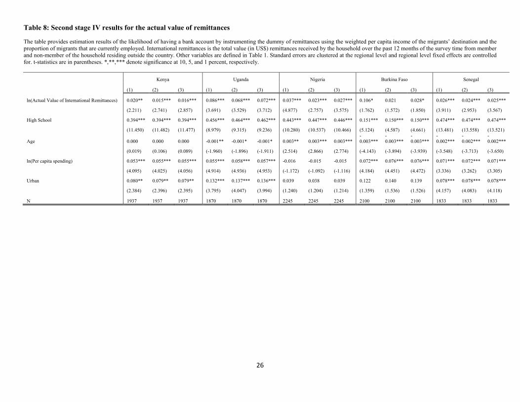
Table 8: Second stage IV results for the actual value of remittances
The table provides estimation results of the likelihood of having a bank account by instrumenting the dummy of remittances using the weighted per capita income of the migrants’ destination and the proportion of migrants that are currently employed. International remittances is the total value (in US$) remittances received by the household over the past 12 months of the survey time from member and non-member of the household residing outside the country. Other variables are defined in Table 1. Standard errors are clustered at the regional level and regional level fixed effects are controlled for. t-statistics are in parentheses. *,**,*** denote significance at 10, 5, and 1 percent, respectively.
Kenya Uganda Nigeria Burkina Faso Senegal
(1) (2) (3) (1) (2) (3) (1) (2) (3) (1) (2) (3) (1) (2) (3)
ln(Actual Value of International Remittances) 0.020** 0.015*** 0.016*** 0.086*** 0.068*** 0.072*** 0.037*** 0.023*** 0.027*** 0.106* 0.021 0.028* 0.026*** 0.024*** 0.025***
(2.211) (2.741) (2.857) (3.691) (3.529) (3.712) (4.877) (2.757) (3.575) (1.762) (1.572) (1.850) (3.911) (2.953) (3.567)
High School 0.394*** 0.394*** 0.394*** 0.456*** 0.464*** 0.462*** 0.443*** 0.447*** 0.446*** 0.151*** 0.150*** 0.150*** 0.474*** 0.474*** 0.474***
(11.450) (11.482) (11.477) (8.979) (9.315) (9.236) (10.280) (10.537) (10.466) (5.124) (4.587) (4.661) (13.481) (13.558) (13.521)
Age 0.000 0.000 0.000 -0.001** -0.001* -0.001* 0.003** 0.003*** 0.003*** -0.003***
-0.003***
-0.003***
-0.002***
-0.002***
-0.002***
(0.019) (0.106) (0.089) (-1.960) (-1.896) (-1.911) (2.514) (2.866) (2.774) (-4.143) (-3.894) (-3.939) (-3.548) (-3.713) (-3.650)
ln(Per capita spending) 0.053*** 0.055*** 0.055*** 0.055*** 0.058*** 0.057*** -0.016 -0.015 -0.015 0.072*** 0.076*** 0.076*** 0.071*** 0.072*** 0.071***
(4.095) (4.025) (4.056) (4.914) (4.936) (4.953) (-1.172) (-1.092) (-1.116) (4.184) (4.451) (4.472) (3.336) (3.262) (3.305)
Urban 0.080** 0.079** 0.079** 0.132*** 0.137*** 0.136*** 0.039 0.038 0.039 0.122 0.140 0.139 0.078*** 0.078*** 0.078***
(2.384) (2.396) (2.395) (3.795) (4.047) (3.994) (1.240) (1.204) (1.214) (1.359) (1.536) (1.526) (4.157) (4.083) (4.118)
N 1937 1937 1937 1870 1870 1870 2245 2245 2245 2100 2100 2100 1833 1833 1833
26

Appendix Table 1: First stage instrumental variable regression results using the dummy of remittances and using sampling weights
The dependent variable is a dummy equal to one if the household received international remittances over the past 12 months, and zero otherwise. The instruments are the weighted per capita income of the migrants’ destination and the proportion of migrants that are currently employed. Other variables are defined in Table 1. Standard errors are clustered at the regional level and region level fixed effects are controlled for and regression is weighted using the relevant sample weights, except for Kenya where results are based on unweighted regressions since the sample is not nationally representative. t-statistics are in parentheses. *,**,*** denote significance at 10, 5, and 1 percent, respectively.
Kenya Uganda Nigeria Burkina Faso Senegal
(1) (2) (3) (1) (2) (3) (1) (2) (3) (1) (2) (3) (1) (2) (3)
High School -0.023 0.002 -0.012 0.070*** 0.059*** 0.057*** -0.004 0.006 0.001 -0.064* -0.002 0.006 0.030 0.142* 0.068
(-1.109) (0.112) (-0.754) (3.317) (3.070) (3.080) (-0.262) (0.598) (0.052) (-2.362) (-0.084) (0.225) (0.463) (2.052) (1.205)
Age -0.001 0.000 -0.001 -0.000 -0.000 -0.000 0.000 0.000 -0.000 0.002*** 0.000 0.000 0.001 0.000 0.001
(-0.892) (0.350) (-1.177) (-0.084) (-0.255) (-0.389) (1.390) (0.645) (-0.024) (3.907) (0.657) (0.949) (0.467) (0.088) (0.617)
ln(Per capita spending) 0.025* 0.026** 0.018* 0.015** 0.009** 0.010** -0.001 0.003 0.003 -0.028 -0.014 -0.017 0.024 0.033** 0.026
(2.096) (2.725) (1.888) (2.565) (2.208) (2.314) (-0.466) (0.870) (0.808) (-1.857) (-1.513) (-1.524) (0.850) (2.267) (1.608)
Urban -0.050** -0.041** -0.037* 0.059** 0.043** 0.041** -0.007 -0.011 -0.010 -0.096* -0.014 -0.027 -0.055 -0.037 -0.040
(-2.413) (-2.143) (-2.064) (2.336) (2.331) (2.219) (-0.998) (-1.452) (-1.315) (-2.366) (-0.568) (-1.622) (-1.380) (-1.299) (-1.261)
Weighted per capita income in migrants’ destination countries 0.017***
0.008*** 0.002***
0.000 0.002***
0.001*** 0.005**
0.003*** 0.003***
0.002***
(15.481)
(6.851) (5.399)
(1.372) (22.510)
(3.947) (3.289)
(6.713) (8.854)
(8.815)
Proportion of migrants abroad currently employed 0.734*** 0.596*** 0.495*** 0.469*** 0.821*** 0.649*** 0.627*** 0.610***
0.732*** 0.558***
(20.283) (13.129) (9.013) (8.433) (17.838) (7.409) (16.197) (15.978)
(18.913) (14.683)
N 1937 1937 1937 1870 1870 1870 2245 2245 2245 2100 2100 2100 1833 1833 1833
Kleibergen-Paap LM Statistic 14.214 15.160 15.239 8.760 17.689 18.399 5.713 4.545 7.839 5.266 4.310 5.347 5.960 7.131 7.238
P-val 0.000 0.000 0.000 0.003 0.000 0.000 0.017 0.033 0.020 0.022 0.038 0.069 0.015 0.008 0.027
Kleibergen-Paap F-Statistic 239.651 411.389 177.783 29.150 81.228 39.392 506.704 318.179 566.992 10.820 262.334 138.192 78.401 357.693 113.300
Hansen J-statistic 0.000 0.000 0.260 0.000 0.000 1.687 0.000 0.000 2.923 0.000 0.000 0.963 0.000 0.000 1.031
P-value
0.610
0.194
0.087
0.326
0.310
Endogeneity test 0.085 0.129 0.045 2.073 0.913 0.528 0.003 1.545 0.208 0.860 0.299 0.108 0.107 0.128 0.579
P-value 0.771 0.720 0.832 0.150 0.339 0.467 0.958 0.214 0.648 0.354 0.584 0.742 0.744 0.720 0.447
27
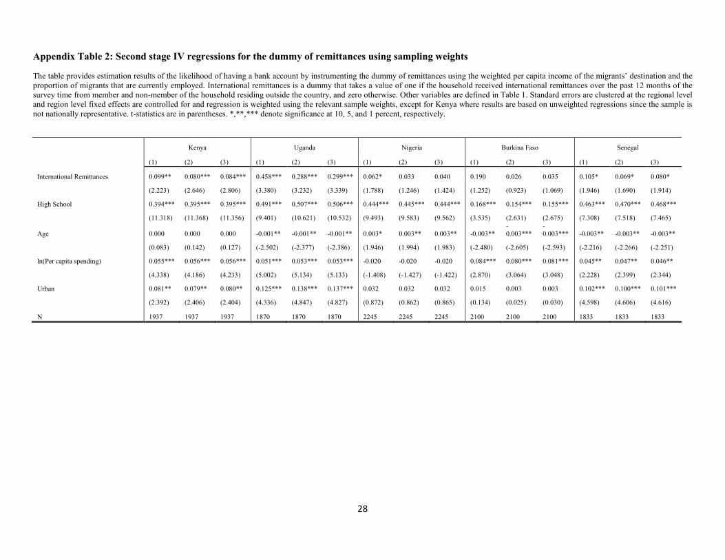
Appendix Table 2: Second stage IV regressions for the dummy of remittances using sampling weights
The table provides estimation results of the likelihood of having a bank account by instrumenting the dummy of remittances using the weighted per capita income of the migrants’ destination and the proportion of migrants that are currently employed. International remittances is a dummy that takes a value of one if the household received international remittances over the past 12 months of the survey time from member and non-member of the household residing outside the country, and zero otherwise. Other variables are defined in Table 1. Standard errors are clustered at the regional level and region level fixed effects are controlled for and regression is weighted using the relevant sample weights, except for Kenya where results are based on unweighted regressions since the sample is not nationally representative. t-statistics are in parentheses. *,**,*** denote significance at 10, 5, and 1 percent, respectively.
Kenya Uganda Nigeria Burkina Faso Senegal
(1) (2) (3) (1) (2) (3) (1) (2) (3) (1) (2) (3) (1) (2) (3)
International Remittances 0.099** 0.080*** 0.084*** 0.458*** 0.288*** 0.299*** 0.062* 0.033 0.040 0.190 0.026 0.035 0.105* 0.069* 0.080*
(2.223) (2.646) (2.806) (3.380) (3.232) (3.339) (1.788) (1.246) (1.424) (1.252) (0.923) (1.069) (1.946) (1.690) (1.914)
High School 0.394*** 0.395*** 0.395*** 0.491*** 0.507*** 0.506*** 0.444*** 0.445*** 0.444*** 0.168*** 0.154*** 0.155*** 0.463*** 0.470*** 0.468***
(11.318) (11.368) (11.356) (9.401) (10.621) (10.532) (9.493) (9.583) (9.562) (3.535) (2.631) (2.675) (7.308) (7.518) (7.465)
Age 0.000 0.000 0.000 -0.001** -0.001** -0.001** 0.003* 0.003** 0.003** -0.003** -0.003***
-0.003*** -0.003** -0.003** -0.003**
(0.083) (0.142) (0.127) (-2.502) (-2.377) (-2.386) (1.946) (1.994) (1.983) (-2.480) (-2.605) (-2.593) (-2.216) (-2.266) (-2.251)
ln(Per capita spending) 0.055*** 0.056*** 0.056*** 0.051*** 0.053*** 0.053*** -0.020 -0.020 -0.020 0.084*** 0.080*** 0.081*** 0.045** 0.047** 0.046**
(4.338) (4.186) (4.233) (5.002) (5.134) (5.133) (-1.408) (-1.427) (-1.422) (2.870) (3.064) (3.048) (2.228) (2.399) (2.344)
Urban 0.081** 0.079** 0.080** 0.125*** 0.138*** 0.137*** 0.032 0.032 0.032 0.015 0.003 0.003 0.102*** 0.100*** 0.101***
(2.392) (2.406) (2.404) (4.336) (4.847) (4.827) (0.872) (0.862) (0.865) (0.134) (0.025) (0.030) (4.598) (4.606) (4.616)
N 1937 1937 1937 1870 1870 1870 2245 2245 2245 2100 2100 2100 1833 1833 1833
28

Appendix Table 3: First stage instrumental variable regressions using actual value of remittances and using sampling weights
The dependent variable is the per capita value (in US$) of international remittances received by household over the past 12 months from members and non-members residing abroad. The independent variables are weighted per capita income of the migrants’ destination and the proportion of migrants that are currently employed. Other variables are defined in Table 1. Standard errors are clustered at the regional level and region level fixed effects are controlled for and regression is weighted using the relevant sample weights, except for Kenya where results are based on unweighted regressions since the sample is not nationally representative. t-statistics are in parentheses. *,**,*** denote significance at 10, 5, and 1 percent, respectively.
Kenya Uganda Nigeria Burkina Faso Senegal
(1) (2) (3) (1) (2) (3) (1) (2) (3) (1) (2) (3) (1) (2) (3)
High School -0.085 0.031 -0.030 0.301*** 0.279*** 0.252*** 0.006 0.045 0.022 -0.088 0.006 0.032 0.163 0.706** 0.294
(-0.770) (0.367) (-0.401) (3.819) (4.363) (4.380) (0.202) (1.050) (0.657) (-0.831) (0.038) (0.243) (0.681) (2.456) (1.356)
Age 0.001 0.004 -0.000 0.001 0.002 0.001 0.003* 0.002 0.002 0.004** 0.001 0.001 -0.002 -0.005 -0.002
(0.280) (1.417) (-0.092) (0.723) (0.989) (0.700) (1.896) (1.419) (1.128) (3.075) (0.387) (0.619) (-0.321) (-0.851) (-0.428)
ln(Per capita spending) 0.235*** 0.229*** 0.193*** 0.090*** 0.069*** 0.072*** 0.032 0.047* 0.045* -0.004 0.024 0.014 0.275** 0.319*** 0.279***
(3.439) (4.427) (3.698) (2.912) (2.852) (3.023) (1.662) (1.841) (1.786) (-0.101) (0.825) (0.450) (2.683) (3.604) (3.894)
Urban -0.232** -0.174 -0.158 0.261** 0.210** 0.195** -0.032 -0.044* -0.041* -0.086 0.075 0.032 -0.386* -0.320* -0.335*
(-2.376) (-1.705) (-1.633) (2.430) (2.583) (2.347) (-1.579) (-1.853) (-1.770) (-0.741) (0.682) (0.341) (-1.816) (-1.862) (-2.139)
Weighted per capita income in migrants’ destination countries 0.086***
0.033*** 0.008***
0.003** 0.009***
0.003*** 0.013***
0.009*** 0.015***
0.009***
(13.057)
(5.110) (5.897)
(2.629) (19.509)
(4.588) (4.646)
(5.498) (7.208)
(6.156)
Proportion of migrants abroad currently employed 3.893*** 3.289*** 1.929*** 1.685*** 2.883*** 2.203*** 1.099*** 1.045***
2.874*** 1.896***
(20.471) (15.412) (7.818) (6.974) (21.336) (9.071) (7.522) (7.213)
(8.309) (7.980)
N 1937 1937 1937 1870 1870 1870 2245 2245 2245 2100 2100 2100 1833 1833 1833
Kleibergen-Paap LM Statistic 14.107 14.797 14.891 7.694 13.493 14.547 5.766 4.805 7.082 4.324 4.166 5.085 5.713 6.516 6.944
P-val 0.000 0.000 0.001 0.006 0.000 0.001 0.016 0.028 0.029 0.038 0.041 0.079 0.017 0.011 0.031
Kleibergen-Paap F-Statistic 170.487 419.081 174.714 34.771 61.120 31.568 380.614 455.226 344.080 21.589 56.577 45.926 51.953 69.040 55.369
Hansen J-statistic 0.000 0.000 0.469 0.000 0.000 0.581 0.000 0.000 2.896 0.000 0.000 1.011 0.000 0.000 0.671
P-value
0.493
0.446
0.089
0.315
0.413
Endogeneity test 0.868 0.186 0.411 1.887 1.282 1.567 0.410 1.302 0.000 0.901 0.037 0.004 0.576 0.119 0.089
P-value 0.352 0.667 0.521 0.170 0.257 0.211 0.522 0.254 0.985 0.343 0.847 0.949 0.448 0.730 0.766
29

Appendix Table 4: Second stage IV results for the actual value of remittances using sampling weights
The table provides second stage IV estimation results of the likelihood of having a bank account by instrumenting the per capita value (in US$) of remittances using the weighted per capita income of the migrants’ destination and the proportion of migrants that are currently employed. International remittances is the actual value of remittances received by household over the past 12 months of the survey time from members and non-members of the household residing outside the country. Other variables are defined in Table 1. Standard errors are clustered at the regional level, region level fixed effects are controlled for and regression is weighted using the relevant sample weights, except for Kenya where results are based on unweighted regressions since the sample is not nationally representative. t-statistics are in parentheses. *,**,*** denote significance at 10, 5, and 1 percent, respectively.
Kenya Uganda Nigeria Burkina Faso Senegal
(1) (2) (3) (1) (2) (3) (1) (2) (3) (1) (2) (3) (1) (2) (3)
ln(Actual Value of International Remittances) 0.020** 0.015*** 0.016*** 0.093*** 0.074*** 0.077*** 0.017* 0.009 0.012 0.077 0.015 0.023 0.023* 0.017* 0.020*
(2.211) (2.741) (2.857) (3.627) (3.410) (3.751) (1.817) (1.253) (1.456) (1.352) (0.939) (1.136) (1.903) (1.751) (1.943)
High School 0.394*** 0.394*** 0.394*** 0.495*** 0.503*** 0.502*** 0.444*** 0.444*** 0.444*** 0.163*** 0.154*** 0.155*** 0.462*** 0.468*** 0.465***
(11.450) (11.482) (11.477) (9.743) (10.628) (10.465) (9.472) (9.574) (9.547) (3.175) (2.643) (2.716) (7.082) (7.327) (7.224)
Age 0.000 0.000 0.000 -0.002*** -0.001*** -0.001*** 0.003* 0.003** 0.003** -0.003*** -0.003*** -0.003*** -0.003** -0.003** -0.003**
(0.019) (0.106) (0.089) (-2.773) (-2.612) (-2.645) (1.917) (1.977) (1.961) (-2.610) (-2.611) (-2.594) (-2.128) (-2.219) (-2.177)
ln(Per capita spending) 0.053*** 0.055*** 0.055*** 0.049*** 0.051*** 0.051*** -0.020 -0.020 -0.020 0.079*** 0.080*** 0.080*** 0.041* 0.044** 0.043**
(4.095) (4.025) (4.056) (4.897) (4.917) (4.933) (-1.477) (-1.468) (-1.470) (3.056) (3.074) (3.075) (1.905) (2.102) (2.011)
Urban 0.080** 0.079** 0.079** 0.128*** 0.135*** 0.133*** 0.032 0.032 0.032 0.003 0.001 0.001 0.106*** 0.103*** 0.104***
(2.384) (2.396) (2.395) (4.580) (4.805) (4.791) (0.872) (0.863) (0.866) (0.026) (0.011) (0.013) (4.489) (4.576) (4.551)
N 1937 1937 1937 1870 1870 1870 2245 2245 2245 2100 2100 2100 1833 1833 1833
30
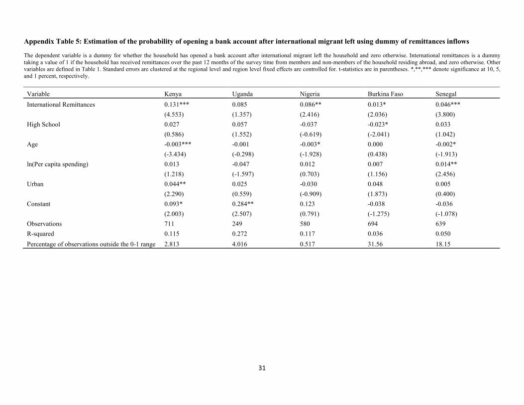
Appendix Table 5: Estimation of the probability of opening a bank account after international migrant left using dummy of remittances inflows
The dependent variable is a dummy for whether the household has opened a bank account after international migrant left the household and zero otherwise. International remittances is a dummy taking a value of 1 if the household has received remittances over the past 12 months of the survey time from members and non-members of the household residing abroad, and zero otherwise. Other variables are defined in Table 1. Standard errors are clustered at the regional level and region level fixed effects are controlled for. t-statistics are in parentheses. *,**,*** denote significance at 10, 5, and 1 percent, respectively. Variable Kenya Uganda Nigeria Burkina Faso Senegal International Remittances 0.131*** 0.085 0.086** 0.013* 0.046***
(4.553) (1.357) (2.416) (2.036) (3.800)
High School 0.027 0.057 -0.037 -0.023* 0.033
(0.586) (1.552) (-0.619) (-2.041) (1.042)
Age -0.003*** -0.001 -0.003* 0.000 -0.002*
(-3.434) (-0.298) (-1.928) (0.438) (-1.913)
ln(Per capita spending) 0.013 -0.047 0.012 0.007 0.014**
(1.218) (-1.597) (0.703) (1.156) (2.456)
Urban 0.044** 0.025 -0.030 0.048 0.005
(2.290) (0.559) (-0.909) (1.873) (0.400)
Constant 0.093* 0.284** 0.123 -0.038 -0.036
(2.003) (2.507) (0.791) (-1.275) (-1.078)
Observations 711 249 580 694 639 R-squared 0.115 0.272 0.117 0.036 0.050 Percentage of observations outside the 0-1 range 2.813 4.016 0.517 31.56 18.15
31

Appendix Table 6: Estimation of the probability of opening a bank account after international migrant left using actual value of remittances
The dependent variable is a dummy for whether the household has opened a bank account after international migrant left the household and zero otherwise. International remittances is a per capita value (in US$) of remittances received by the household over the past 12 months of the survey time from member and non-member household residing abroad. Other variables are defined in Table 1. Standard errors are clustered at the regional level and region level fixed effects are controlled for. t-statistics are in parentheses. *,**,*** denote significance at 10, 5, and 1 percent, respectively. Variable Kenya Uganda Nigeria Burkina Faso Senegal ln(Actual Value of International Remittances) 0.022*** 0.019** 0.032*** 0.009* 0.014***
(4.390) (2.308) (3.241) (1.963) (4.557)
High School 0.021 0.052 -0.047 -0.025** 0.033
(0.476) (1.593) (-0.830) (-2.509) (1.002)
Age -0.003*** -0.001 -0.004** 0.000 -0.002*
(-3.611) (-0.462) (-2.466) (0.326) (-2.015)
ln(Per capita spending) 0.009 -0.050 -0.001 0.006 0.007
(0.847) (-1.675) (-0.046) (1.036) (1.335)
Urban 0.040* 0.022 -0.037 0.043 0.006
(2.069) (0.536) (-1.218) (1.723) (0.514)
Constant 0.142*** 0.316*** 0.222 -0.032 -0.010
(2.977) (2.817) (1.544) (-1.169) (-0.306)
Observations 711 249 580 694 639 R-squared 0.114 0.274 0.142 0.048 0.068 Percentage of observations outside the 0-1 range 2.110 4.016 3.793 45.53 25.51
32