International Portfolio Flows and FDI Flows: “Hot” or “Cold? ”

By

Itay Goldstein and Assaf Razin

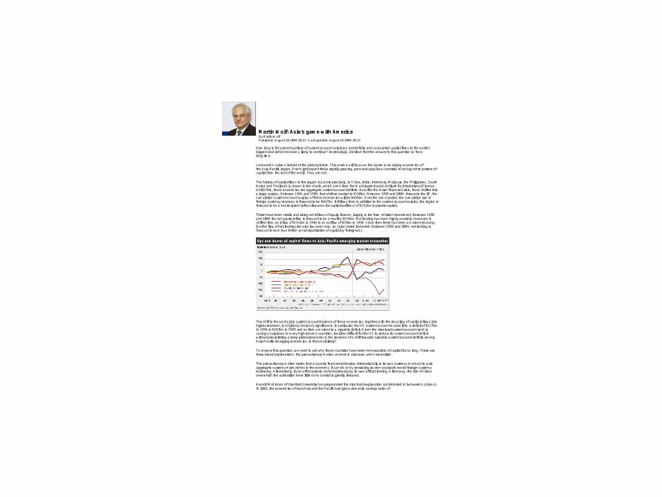
Martin Wolf: Asia's game with America By Martin Wolf Published: August 10 2004 20:15 | Last updated: August 10 2004 20:15

How long is the present pattern of current account surpluses and deficits and associated capital flows to the world's biggest and richest economy likely to continue? Increasingly, I believe that the answer to this question is: for a long time.

Last week's column looked at the global picture. This week's will focus on the dynamic emerging economies of the Asia-Pacific region. One might expect these rapidly growing, poor and populous countries to be big net importers of capital from the rest of the world. They are not.

The history of capital flows to the region (or, more precisely, to China, India, Indonesia, Malaysia, the Philippines, South Korea and Thailand) is shown in the charts, which come from the Washington-based Institute for International Finance. Until 1996, these economies ran aggregate current account deficits. But after the Asian financial crisis, these shifted into a large surplus. Between 1996 and 1998, that shift amounted to $150bn. Between 1998 and 2004, forecasts the IIF, the cumulative current account surplus of these economies will be $495bn. Over the same period, the cumulative rise in foreign currency reserves is forecast to be $647bn. It follows that, in addition to the current account surplus, the region is forecast to be a net recipient (after allowance for capital outflows) of $152bn in private capital.

There have been stable and rising net inflows of equity finance, largely in the form of direct investment. Between 1998 and 2004 the net equity inflow is forecast to be a healthy $516bn. Net lending has been highly unstable, however: it shifted from an inflow of $116bn in 1996 to an outflow of $59bn in 1998. Since then there has been a modest recovery. But the flow of net lending remains low even now, as I also noted last week. Between 1998 and 2004, net lending is forecast to be minus $58bn (a net repatriation of capital by foreigners).

The shift in the post-crisis current account balance of these economies, together with the recycling of capital inflows into higher reserves, is of global, not local, significance. In particular, the US current account moved from a deficit of $117bn in 1996 to $291bn in 1999 and so from a modest to a sizeable deficit. Given the structural current account (and so savings) surpluses in many high-income countries, it will be difficult for the US to reduce its current account deficit without precipitating a deep global recession in the absence of a shift towards sizeable current account deficits among Asia-Pacific emerging economies. Is that at all likely?

To answer this question, we need to ask why these countries have been net exporters of capital for so long. There are three broad explanations: the precautionary motive; economic structure; and mercantilism.

The precautionary motive states that a country that cannot borrow internationally in its own currency must act to curb aggregate currency mismatches in the economy. It can do so by restricting its own or private sector foreign currency borrowing. Alternatively, it can offset private sector borrowing by its own official lending. Either way, the risk of crises over which the authorities have little or no control is greatly reduced.

Ronald McKinnon of Stanford University has propounded the structural explanation (as indicated in last week's column). In 2002, the economies of east Asia and the Pacific had gross domestic savings rates of

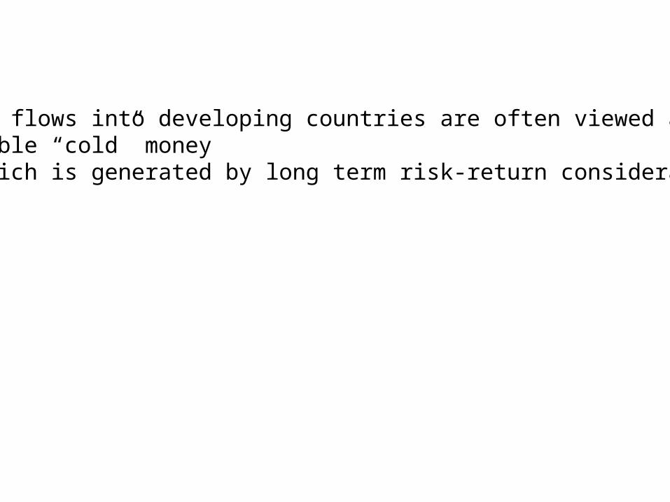
FDI flows into developing countries are often viewed as stable “cold” money

Which is generated by long term risk-return considerations.

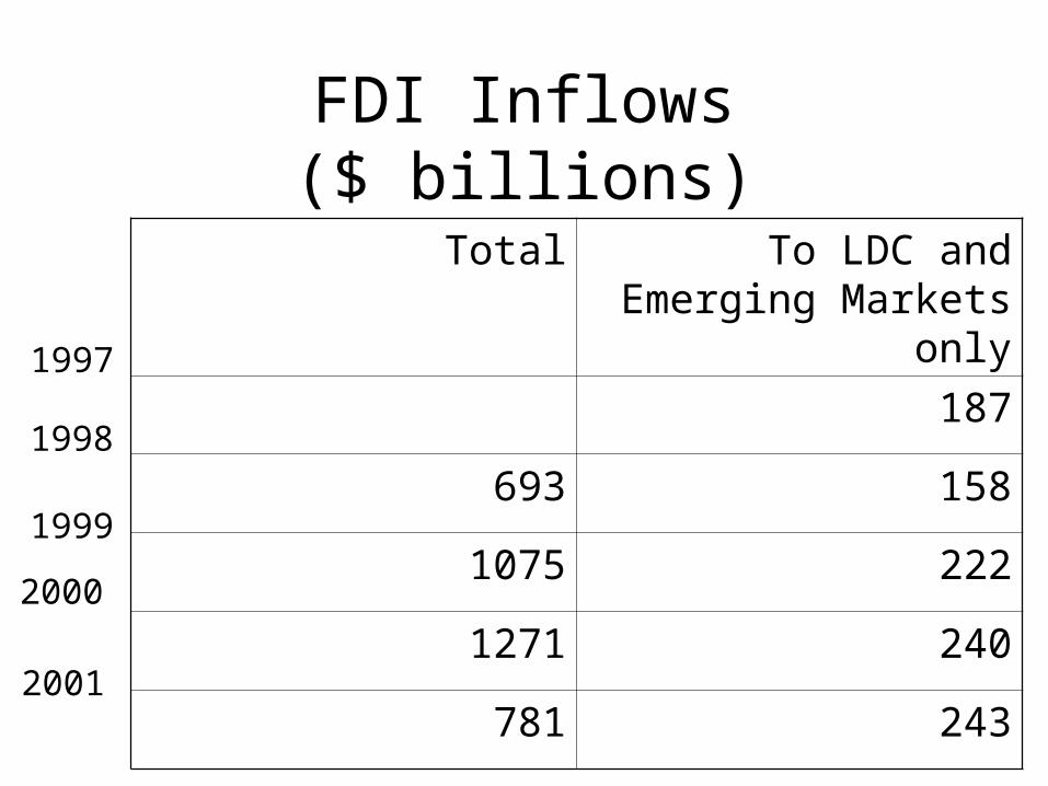
FDI Inflows($ billions)

To LDC and Emerging Markets only

Total

187

158693

2221075

2401271

243781

1997

1998

1999

2000

2001

• “Imagine a large company that has many relatively small shareholders.Then, each

shareholder faces the following well-known free-rider problem:if the shareholder does

something to improve the quality of management, then the benefits will be enjoyed

by all shareholders. Unless the shareholder is altruistic, she will ignore this beneficial effect on other shareholders and so will under-invest

in the activity of monitoring or improving management.” Oliver Hart.

Efficiency vs. Excessive Information?

•“A distinction is often made between short-term and long-term capital flows: the former are deemed unstable hot money and the

latter are deemed stable cold money. Using time-series analysis of balance of payments data for five industrial countries and five

developing countries, we find that in most cases the labels “short term” and “long term” do not convey any information about the

time-series properties of the flow. In particular, long-term flows are often as volatile and unpredictable as short-term flows”.

•We address the question: Which is more volatile—FDI flows or Equity Portfolio flows?

With controlling shares FDI investor will devote time and resources to persuading other shareholders of a company to replace incompetent management. As a result the management of a company will be under pressure to perform well.

However, when investors want to sell their investment ,they will get lower price if they have more information.

Because, other investors knowThat the seller has information on the

Fundamentals and suspectThat the sales result from bad prospects of the projectRather than liquidity shortage.

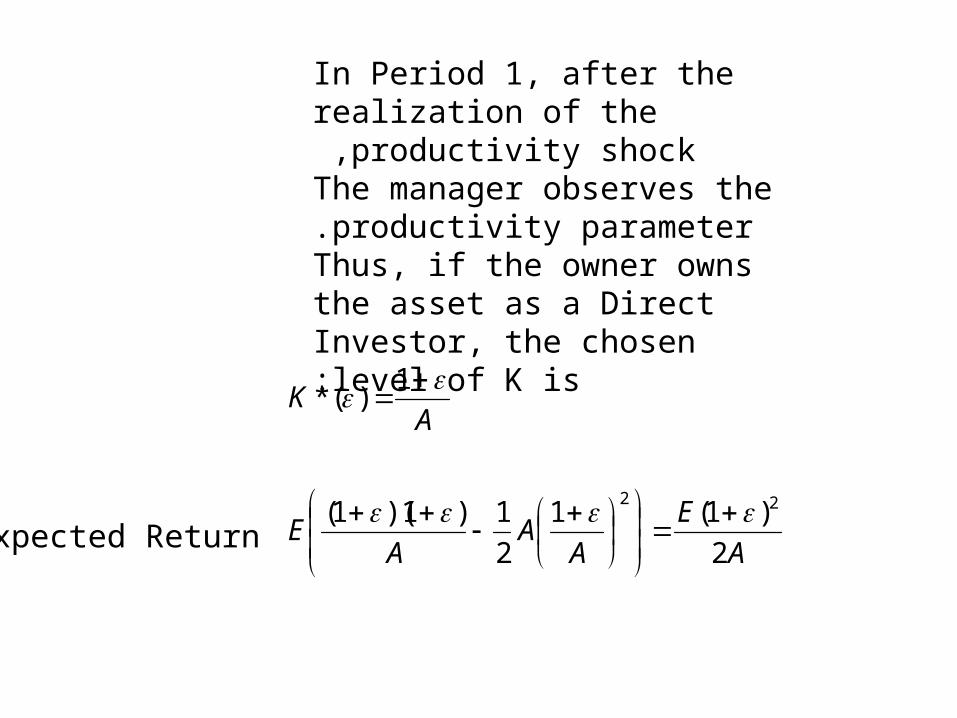
In Period 1, after the realization of the productivity shock ,

The manager observes the productivity parameter.

Thus, if the owner owns the asset as a Direct Investor, the chosen level of K is:

A

E

AA

AE

AK

2

)1(1

2

1)1)(1(

1)(*

22

Expected Return

Liquidity Shocks and Resale Values

2

2

1)1(

)(')(,1)1(,0)1(),(

)1)((

AKKR

GgGGGcdf

KFR

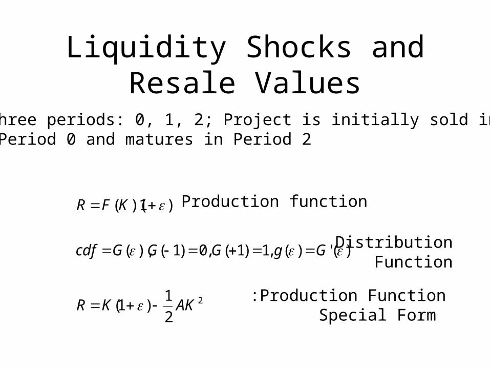
Three periods: 0, 1, 2; Project is initially sold inPeriod 0 and matures in Period 2.

Production function

Distribution Function

Production Function: Special Form

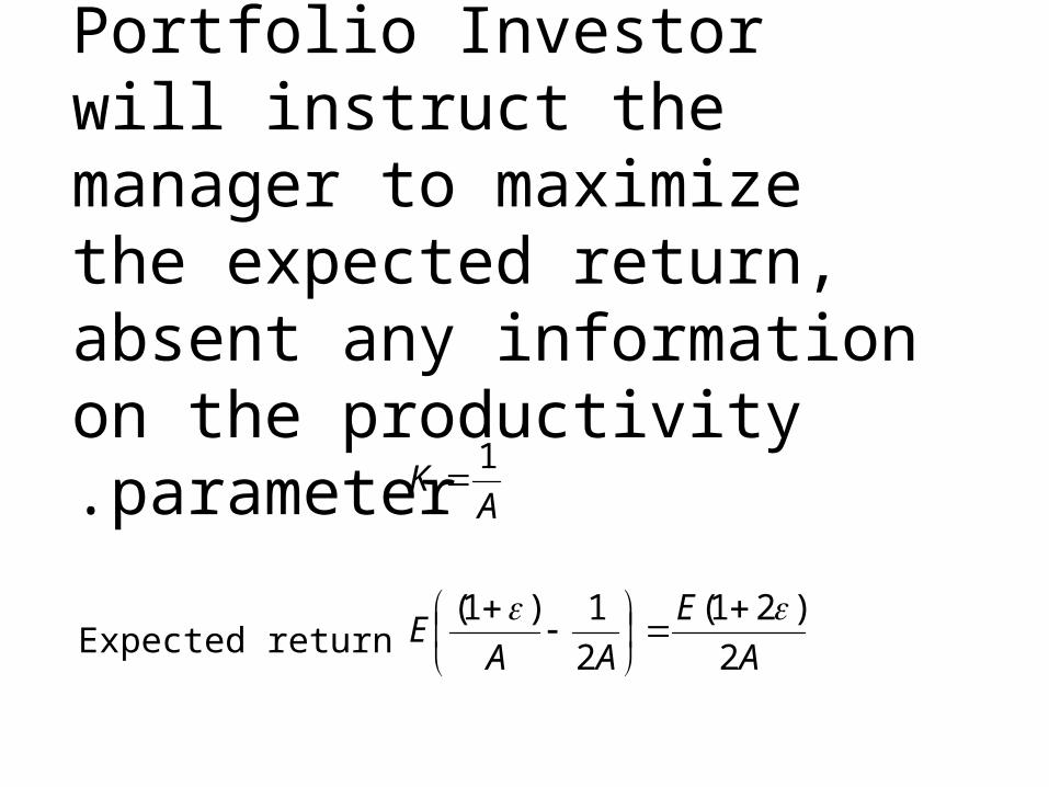
Portfolio Investor will instruct the manager to maximize the expected return, absent any information on the productivity parameter.

A

E

AAE

AK

2

)21(

2

1)1(

1

Expected return

Liquidity Shocks and Re-sales

AP

G

dgA

dgA

P

Gyprobabilit

threshold

DD

DD

D

D

D

2

)1(

)()1(

)(2

21)(

2)1(

)1(

)()1(

2

,1

1

1

1

2

,1

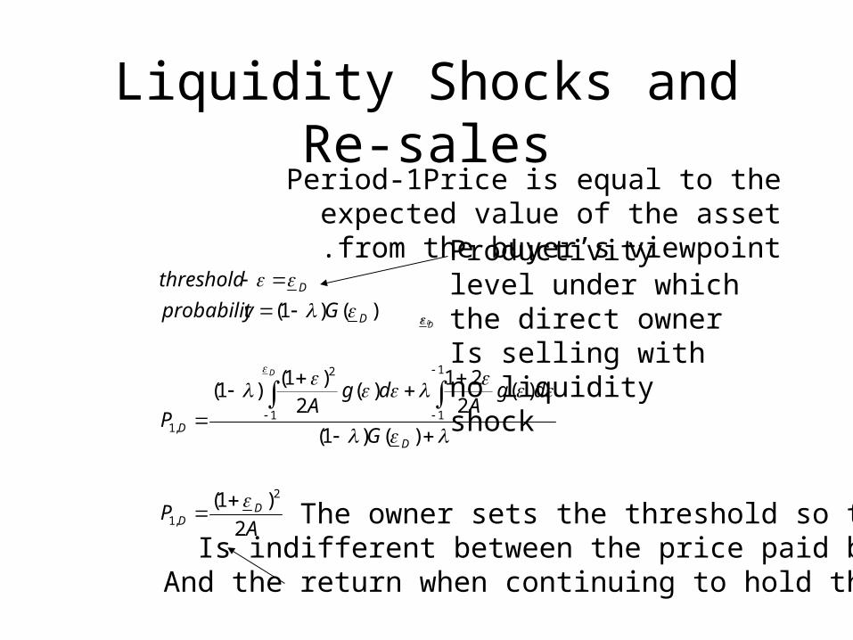
Period-1Price is equal to the expected value of the asset from the buyer’s viewpoint.

Productivity level under which the direct ownerIs selling with no liquidity shock

The owner sets the threshold so that she Is indifferent between the price paid by buyer

And the return when continuing to hold the asset

DD

PDD

P

PA

P

Adg

AP

,1,1

1

1

,1

2

10

2

1)(

2

21

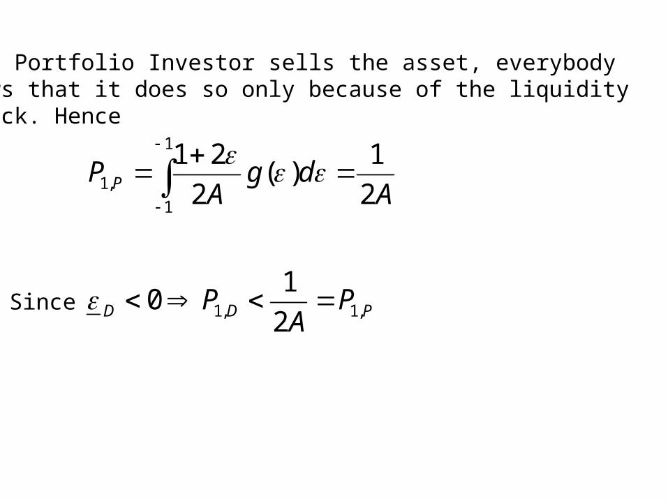
If a Portfolio Investor sells the asset, everybodyknows that it does so only because of the liquidity

shock. Hence:

Since

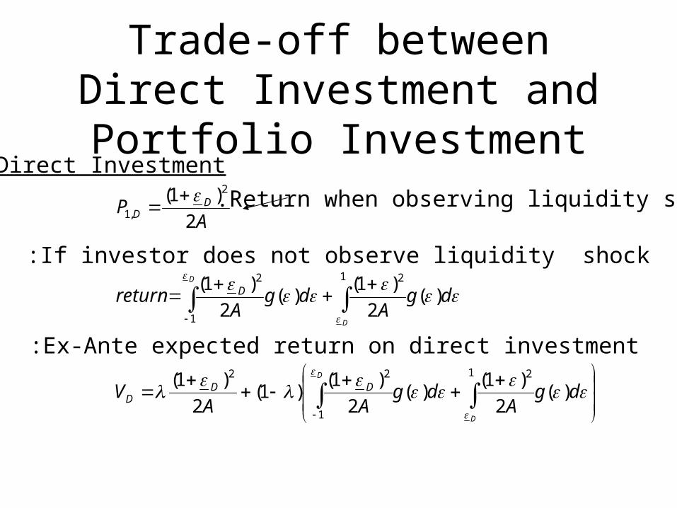
Trade-off between Direct Investment and Portfolio

Investment

dgA

dgAA

V

dgA

dgA

return

AP

D

D

D

D

DDD

D

DD

)(2

)1()(

2

)1()1(

2

)1(

)(2

)1()(

2

)1(

2

)1(

1 2

1

22

1 2

1

2

2

,1

If investor does not observe liquidity shock:

Ex-Ante expected return on direct investment:

Direct Investment

Return when observing liquidity shock.

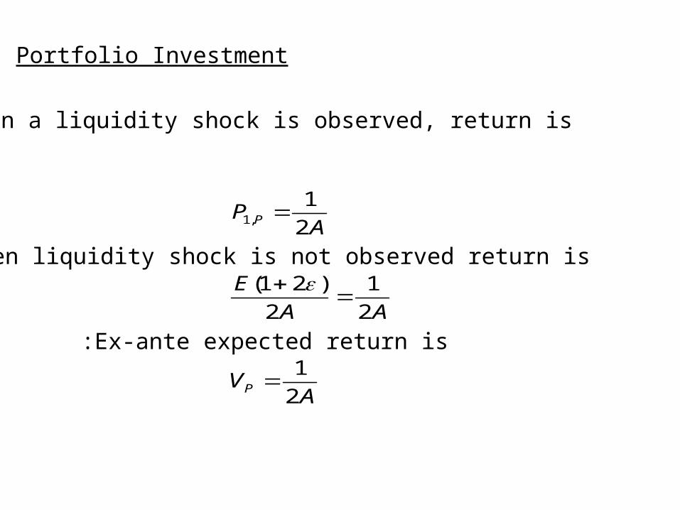
Portfolio Investment

AV

AA

E

AP

P

P

2

1

2

1

2

)21(

2

1,1

When a liquidity shock is observed, return is:

When liquidity shock is not observed return is:

Ex-ante expected return is:

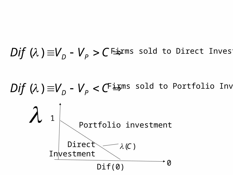
CVVDif

CVVDif

PD

PD

)(

)(

Firms sold to Direct Investor

Firms sold to Portfolio Investor

0

1

Dif(0)

Direct Investment

Portfolio investment

)(C

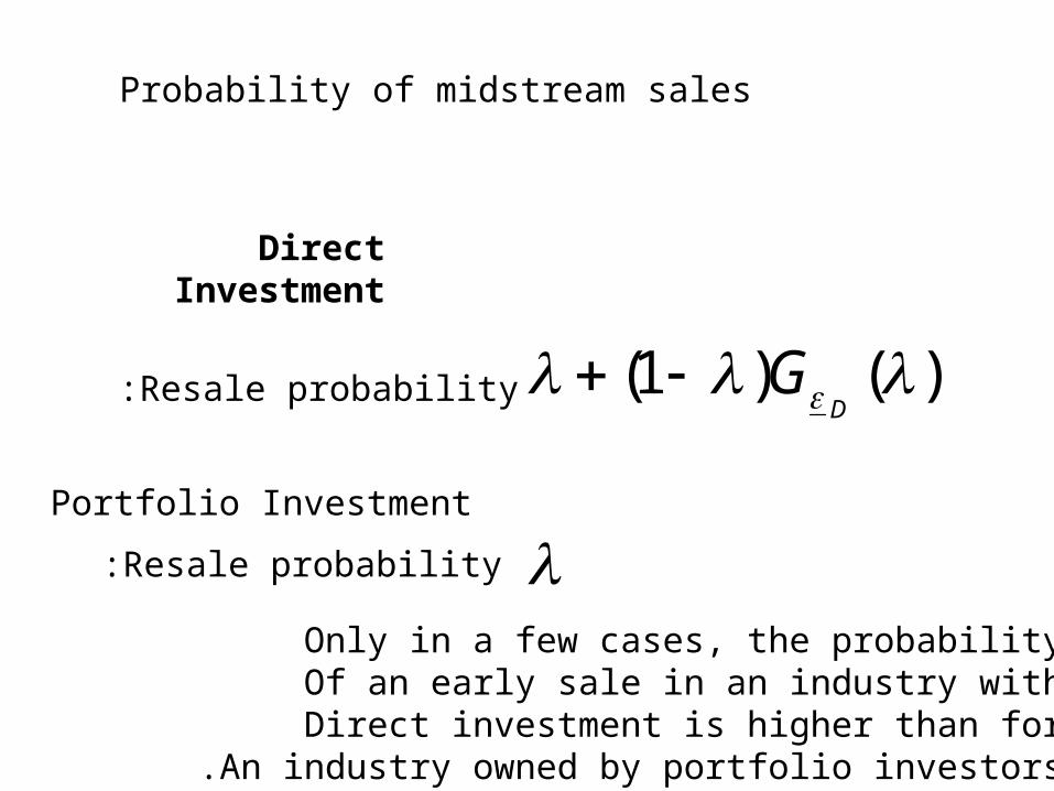
Probability of midstream sales

Direct Investment

)()1(D

GResale probability:

Portfolio Investment

Resale probability:

Only in a few cases, the probabilityOf an early sale in an industry with Direct investment is higher than for

An industry owned by portfolio investors.

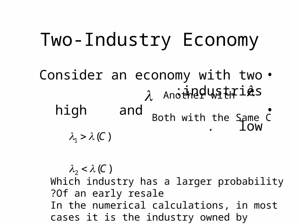
Two-Industry Economy

•Consider an economy with two industries :•high and low .

Both with the Same C

Another with

)(

)(

2

1

C

C

Which industry has a larger probability Of an early resale?

In the numerical calculations, in most cases it is the industry owned by portfolio investors.

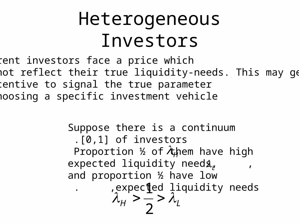
Heterogeneous Investors

Suppose there is a continuum [0,1] of investors .Proportion ½ of them have high

expected liquidity needs, , and proportion ½ have low expected liquidity needs . ,

HL

LH 2

1

Different investors face a price whichDoes not reflect their true liquidity-needs. This may generateAn incentive to signal the true parameterBy choosing a specific investment vehicle.

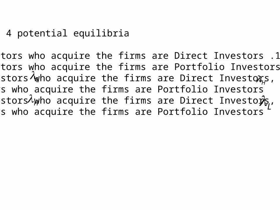
There are 4 potential equilibria:

1 .All investors who acquire the firms are Direct Investors.2 .All investors who acquire the firms are Portfolio Investors.

3 .investors who acquire the firms are Direct Investors, and investors who acquire the firms are Portfolio Investors .

4 .investors who acquire the firms are Direct Investors, and investors who acquire the firms are Portfolio Investors . L

L

HH

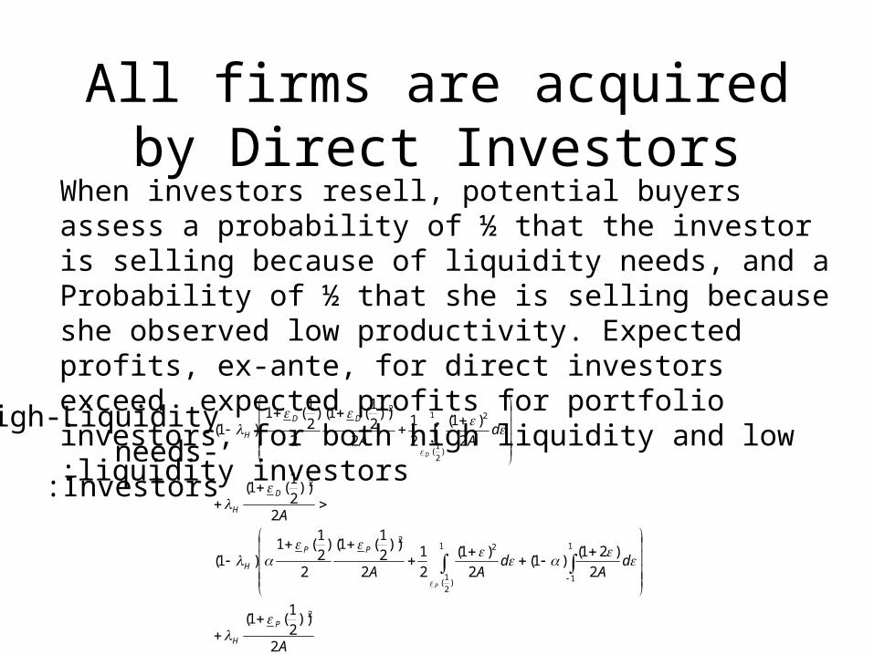
All firms are acquired by Direct Investors

A

dA

dAA

A

dAA

P

H

PP

H

D

H

DD

H

P

D

2

))21

(1(

2

)21()1(

2

)1(

2

1

2

))21

(1(

2

)21

(1)1(

2

))21

(1(

2

)1(

2

1

2

))21

(1(

2

)21

(1)1(

2

1

1

1

)2

1(

22

2

1

)2

1(

22

When investors resell, potential buyers assess a probability of ½ that the investor is selling because of liquidity needs, and a

Probability of ½ that she is selling because she observed low productivity. Expected profits, ex-ante, for direct investors exceed expected profits for portfolio investors, for both high liquidity and low liquidity investors:

High-Liquidity-needs

Investors:

A

dA

dAA

A

dAA

P

L

PP

L

D

L

DD

L

P

D

2

))21

(1(

2

)21()1(

2

)1(

2

1

2

))21

(1(

2

)21

(1)1(

2

))21

(1(

2

)1(

2

1

2

))21

(1(

2

)21

(1)1(

2

1

1

1

)2

1(

22

2

1

)2

1(

22

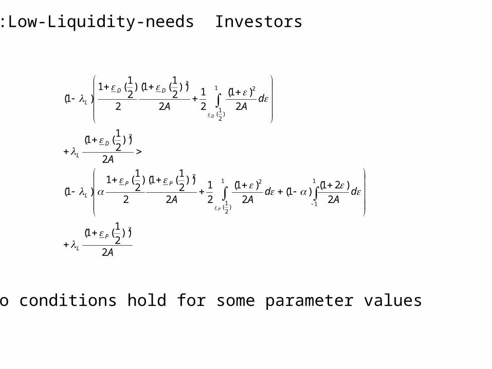
Low-Liquidity-needs Investors:

The two conditions hold for some parameter values!

Other Equilibria:

•Equilibrium 2: All firms are acquired by Portfolio Investors---the two incentive compatibility conditions are not met.

Other Equilibria:•Equilibrium 3: Proportion of Portfolio Investors

and proportion of Direct Investors acquire the firms-----The incentive compatibility conditions are met, for some parameter values.

• Equilibrium 4: Proportion of Portfolio Investors and proportion of Direct Investors acquire the firms----The incentive compatibility conditions are not met.

LH

HL

Two equilibria are possible . Either

(1 )all firms are acquired byDirect Investors,

Or ,

(2 )firms are acquired in the proportion by Portfolio InvestorsAnd in the proportion by Direct

Investors .

L

H

InterpretationThe reason for the existence of the only-direct

investment equilibrium is the strategic externalities between high-liquidity-need Investors .

An investor of this type benefits from having more investors of her type When attempting to resell ,

price does not move against her that much, becausethe “market” knows with high probability thatthe resale is due to liquidity needs.

When all high-liquidity-need investors acquire the firms, a single investor

of this type knows that when resale contingency arises, price will be low, and she will choose

to become a direct investor, self validating the behavior of investors of this type in the

equilibrium. The low-liquidity-need InvestorsCare less about the resale contingency.