
International Journal of Image Processing (IJIP) Volume 4 Issue 6
172
-
Upload
ai-coordinator-csc-journals -
Category
Documents
-
view
222 -
download
0
Transcript of International Journal of Image Processing (IJIP) Volume 4 Issue 6

8/6/2019 International Journal of Image Processing (IJIP) Volume 4 Issue 6
http://slidepdf.com/reader/full/international-journal-of-image-processing-ijip-volume-4-issue-6 1/172

8/6/2019 International Journal of Image Processing (IJIP) Volume 4 Issue 6
http://slidepdf.com/reader/full/international-journal-of-image-processing-ijip-volume-4-issue-6 2/172
International Journal of ImageProcessing (IJIP)
Volume 4, Issue 6, 2011
Edited ByComputer Science Journals
www.cscjournals.org

8/6/2019 International Journal of Image Processing (IJIP) Volume 4 Issue 6
http://slidepdf.com/reader/full/international-journal-of-image-processing-ijip-volume-4-issue-6 3/172
Editor in Chief Professor Hu, Yu-Chen
International Journal of Image Processing
(IJIP)Book: 2011 Volume 4, Issue 6
Publishing Date: 08-02-2011
Proceedings
ISSN (Online): 1985-2304
This work is subjected to copyright. All rights are reserved whether the whole or
part of the material is concerned, specifically the rights of translation, reprinting,re-use of illusions, recitation, broadcasting, reproduction on microfilms or in any
other way, and storage in data banks. Duplication of this publication of parts
thereof is permitted only under the provision of the copyright law 1965, in its
current version, and permission of use must always be obtained from CSC
Publishers. Violations are liable to prosecution under the copyright law.
IJIPJournal is a part of CSC Publishers
http://www.cscjournals.org
© IJIP Journal
Published in Malaysia
Typesetting: Camera-ready by author, data conversation by CSC Publishing
Services – CSC Journals, Malaysia
CSC Publishers

8/6/2019 International Journal of Image Processing (IJIP) Volume 4 Issue 6
http://slidepdf.com/reader/full/international-journal-of-image-processing-ijip-volume-4-issue-6 4/172
Editorial Preface
The International Journal of Image Processing (IJIP) is an effective mediumfor interchange of high quality theoretical and applied research in the ImageProcessing domain from theoretical research to application development. Thisis the fifth issue of volume four of IJIP. The Journal is published bi-monthly,with papers being peer reviewed to high international standards. IJIPemphasizes on efficient and effective image technologies, and provides acentral for a deeper understanding in the discipline by encouraging thequantitative comparison and performance evaluation of the emergingcomponents of image processing. IJIP comprehensively cover the system,processing and application aspects of image processing. Some of theimportant topics are architecture of imaging and vision systems, chemicaland spectral sensitization, coding and transmission, generation and display,image processing: coding analysis and recognition, photopolymers, visualinspection etc.
IJIP give an opportunity to scientists, researchers, engineers and vendorsfrom different disciplines of image processing to share the ideas, identifyproblems, investigate relevant issues, share common interests, explore newapproaches, and initiate possible collaborative research and systemdevelopment. This journal is helpful for the researchers and R&D engineers,scientists all those persons who are involve in image processing in anyshape.
Highly professional scholars give their efforts, valuable time, expertise andmotivation to IJIP as Editorial board members. All submissions are evaluated
by the International Editorial Board. The International Editorial Board ensuresthat significant developments in image processing from around the world arereflected in the IJIP publications.
IJIP editors understand that how much it is important for authors andresearchers to have their work published with a minimum delay aftersubmission of their papers. They also strongly believe that the directcommunication between the editors and authors are important for thewelfare, quality and wellbeing of the Journal and its readers. Therefore, allactivities from paper submission to paper publication are controlled throughelectronic systems that include electronic submission, editorial panel andreview system that ensures rapid decision with least delays in the publicationprocesses.

8/6/2019 International Journal of Image Processing (IJIP) Volume 4 Issue 6
http://slidepdf.com/reader/full/international-journal-of-image-processing-ijip-volume-4-issue-6 5/172
To build its international reputation, we are disseminating the publicationinformation through Google Books, Google Scholar, Directory of Open AccessJournals (DOAJ), Open J Gate, ScientificCommons, Docstoc and many more.Our International Editors are working on establishing ISI listing and a goodimpact factor for IJIP. We would like to remind you that the success of our
journal depends directly on the number of quality articles submitted forreview. Accordingly, we would like to request your participation bysubmitting quality manuscripts for review and encouraging your colleagues tosubmit quality manuscripts for review. One of the great benefits we canprovide to our prospective authors is the mentoring nature of our reviewprocess. IJIP provides authors with high quality, helpful reviews that areshaped to assist authors in improving their manuscripts.
Editorial Board MembersInternational Journal of Image Processing (IJIP)

8/6/2019 International Journal of Image Processing (IJIP) Volume 4 Issue 6
http://slidepdf.com/reader/full/international-journal-of-image-processing-ijip-volume-4-issue-6 6/172
Editorial Board
Editor-in-Chief (EiC)Professor Hu, Yu-Chen
Providence University (Taiwan)
Associate Editors (AEiCs)Professor. Khan M. IftekharuddinUniversity of Memphis (United States of America)Dr. Jane(Jia) YouThe Hong Kong Polytechnic University (China)Professor. Davide La TorreUniversity of Milan (Italy)Professor. Ryszard S. ChorasUniversity of Technology & Life Sciences (Poland)Dr. Huiyu Zhou
Queen’s University Belfast (United Kindom)Professor Yen-Wei ChenRitsumeikan University (Japan)
Editorial Board Members (EBMs)Assistant Professor. M. Emre CelebiLouisiana State University in Shreveport (United States of America) Professor. Herb KunzeUniversity of Guelph (Canada)Professor Karray FakhreddineUniversity of Waterloo (United States of America) Assistant Professor. Yufang Tracy Bao
Fayetteville State University (North Carolina)Dr. C. Saravanan National Institute of Technology, Durgapur West Benga (India)Dr. Ghassan Adnan Hamid Al-KindiSohar University (Oman)Dr. Cho Siu Yeung DavidNanyang Technological University (Singapore)Dr. E. Sreenivasa ReddyVasireddy Venkatadri Institute of Technology (India)Dr. Khalid Mohamed HosnyZagazig University (Egypt)Dr. Gerald SchaeferLoughborough University (United Kingdom)[
Dr. Chin-Feng LeeChaoyang University of Technology (Taiwan)[
Associate Professor. Wang, Xao-NianTong Ji University (China)[ Professor. Yongping Zhang Ningbo University of Technology (China) Professor Santhosh.P.MathewMahatma Gandhi University (India)

8/6/2019 International Journal of Image Processing (IJIP) Volume 4 Issue 6
http://slidepdf.com/reader/full/international-journal-of-image-processing-ijip-volume-4-issue-6 7/172
International Journal of Image Processing (IJIP) ,Volume (4): Issue (6)
Table of Content
Volume 4, Issue 6, December 2011
Pages
518-538 Omnidirectional Thermal Imaging Surveillance System
Featuring Trespasser and Faint Detection
Wong Wai Kit, Zeh-Yang Chew, Hong-Liang Lim, Chu-Kiong
Loo, Way-Soong Lim
539 -548 A Novel Cosine Approximation for High-Speed Evaluation of DCT
Geetha Komandur, M. UttaraKumari
549-556 An Evolutionary Dynamic Clustering based Colour ImageSegmentation Amiya Halder, Nilvra Pathak
557-566 Towards Semantic Clustering -A Review
Phei-Chin Lim, Narayanan Kulathuramaiyer, Dayang
NurFatimah Awg. Iskandar
567-583 Road Sign Detection and Recognition by using Local Energy BasedShape Histogram (LESH)
Usman Zakir, Iffat Zafar, Eran A. Edirisinghe
584 -599 Assessment of Vascular Network Segmentation Jack Collins, Christopher Kurcz, Curtis Lisle, Yanling Liu,
Enrique Zudaire
8/6/2019 International Journal of Image Processing (IJIP) Volume 4 Issue 6
http://slidepdf.com/reader/full/international-journal-of-image-processing-ijip-volume-4-issue-6 8/172
International Journal of Image Processing (IJIP) ,Volume (4): Issue (6)
600-609 Colour Face Image Database for Skin Segmentation, FaceDetection, Recognition and Tracking of Black Faces Under Real-Life Situations OJO, John Adedapo, Adeniran, Solomon A
610-619 Rate Distortion Performance for Joint Source Channel Coding ofJPEG image Over AWGN Channel Jigisha N. Patel, Suprava Patnaik, Vaibhavi P. Lineswala
620-630 Improving Performance of Multileveled BTC Based CBIR UsingSundry Color Spaces
H.B.Kekre, Sudeep D.Thepade, Srikant Sanas
631-646 A Hybrid Trademark Retrieval System Using Four-Gray-LevelZernike Moments and Image Compactness Indices Kazi Mostafa, Huan-Kai Hung, Innchyn Her
647-660 Statistical Models for Face Recognition System With DifferentDistance Measures R.Thiyagarajan, S. Arulselvi, G.Sainarayanan
661-668 A Novel Approach for Cancer Detection in MRI Mammogram UsingDecision Tree Induction and BPN
S. Pitchumani Angayarkanni, V. Saravanan
669-676 Method for Real Time Text Extraction of Digital Manga Comic
Kohei Arai, Herman Tolle
8/6/2019 International Journal of Image Processing (IJIP) Volume 4 Issue 6
http://slidepdf.com/reader/full/international-journal-of-image-processing-ijip-volume-4-issue-6 9/172
Wai-Kit Wong, Zeh-Yang Chew, Hong-Liang Lim, Chu-Kiong Loo & Way-Soong Lim
International Journal of Image Processing (IJIP), Volume (4): Issue (6) 518
Omnidirectional Thermal Imaging Surveillance SystemFeaturing Trespasser and Faint Detection
Wai-Kit Wong [email protected] Faculty of Engineering and Technology,Multimedia University,
75450 JLN Ayer Keroh Lama,Melaka, Malaysia.
Zeh-Yang Chew [email protected] Faculty of Engineering and Technology,Multimedia University,75450 JLN Ayer Keroh Lama,Melaka, Malaysia.
Hong-Liang Lim [email protected] Faculty of Engineering and Technology,Multimedia University,75450 JLN Ayer Keroh Lama,
Melaka, Malaysia.
Chu-Kiong Loo [email protected] Faculty of Engineering and Technology,Multimedia University,75450 JLN Ayer Keroh Lama,Melaka, Malaysia.
Way-Soong Lim [email protected] Faculty of Engineering and Technology,Multimedia University,75450 JLN Ayer Keroh Lama,Melaka, Malaysia.
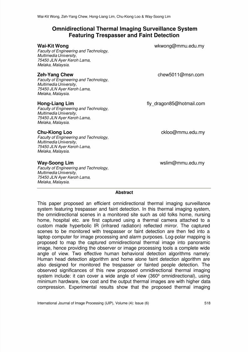
Abstract
This paper proposed an efficient omnidirectional thermal imaging surveillancesystem featuring trespasser and faint detection. In this thermal imaging system,the omnidirectional scenes in a monitored site such as old folks home, nursinghome, hospital etc. are first captured using a thermal camera attached to acustom made hyperbolic IR (infrared radiation) reflected mirror. The capturedscenes to be monitored with trespasser or faint detection are then fed into alaptop computer for image processing and alarm purposes. Log-polar mapping isproposed to map the captured omnidirectional thermal image into panoramicimage, hence providing the observer or image processing tools a complete wideangle of view. Two effective human behavioral detection algorithms namely:Human head detection algorithm and home alone faint detection algorithm arealso designed for monitored the trespasser or fainted people detection. Theobserved significances of this new proposed omnidirectional thermal imagingsystem include: it can cover a wide angle of view (360º omnidirectional), usingminimum hardware, low cost and the output thermal images are with higher datacompression. Experimental results show that the proposed thermal imaging

8/6/2019 International Journal of Image Processing (IJIP) Volume 4 Issue 6
http://slidepdf.com/reader/full/international-journal-of-image-processing-ijip-volume-4-issue-6 10/172
Wai-Kit Wong, Zeh-Yang Chew, Hong-Liang Lim, Chu-Kiong Loo & Way-Soong Lim
International Journal of Image Processing (IJIP), Volume (4): Issue (6) 519
surveillance system achieves high accuracy in detecting trespasser andmonitoring faint detection for health care purpose.
Keywords: Monitoring and Surveillance, Thermal Imaging System, Trespasser Detection, FaintDetection, Omnidirectional System, Image Processing and Understanding.
1. INTRODUCTIONConventional surveillance system that employs digital security cameras are great to keepresidences safe from thief, vandalism, unwanted intruders and at the meantime can work as ahealth care facility for nursing purposes. However, such surveillance system normally employshuman observers to analyze the surveillance video. Sometime this is more prone to error due tolapses in attention of the human observer [1]. There is a fact that a human’s visual attention dropsbelow acceptable levels when assigned to visual monitoring and this fact holds true even for atrained personnel [2],[3]. The weakness in conventional surveillance system has raised the needfor a smart surveillance system where it employs computer and pattern recognition techniques toanalyze information from situated sensors [4].
Another problem encountered in most conventional surveillance systems is the change inambient light, especially in an outdoor environment where the lighting condition is varies naturally.
This makes the conventional digital color images analysis task very difficult. One commonapproach to alleviate this problem is to train the system to compensate for any change in theillumination [5]. However, this is generally not enough for human detection in dark. In recent time,thermal camera has been used for imaging objects in the dark. The camera uses infrared (IR)sensors that capture IR radiation coming from different objects in the surrounding and forms IRimage [6]. Since IR radiation from an object is due to the thermal radiation, and not the lightreflected from the object, such camera can be conveniently used for trespasser or faint detectionin night vision too.
Thermal imaging trespasser detection system is a type of smart surveillance system which isused to detect human objects (trespasser) even in poor lighting condition. The system can beemployed to secure a place when and where human should not exist. A simple trespasserdetection algorithm was proposed in [7]. The algorithm is regional based whereby an IR object
that occupy more than certain number of partitions in a thermal image is considered as a humanbeing and vice-versa. However, the algorithm is having two major concerns. First concern isdistance, in which if a human being that is far away from the imaging system will not identified asa human. The second concern is if an animal (such as cat, dog etc.) is moving too close to thesystem (which occupy more than the threshold partitioned), it will be miss-considered as a humanbeing too. Therefore, in this paper, a more effective trespasser detection algorithm with humanhead detection capability is proposed.
The second approach for the proposed omnidirectional thermal imaging surveillance system inthis paper is with faint detection feature. Faint is one of the major problems that happen amongstthe elderly people, patients or pregnant women which may cause them suffering physical injuriesor even mental problems. Fainting normally occurs when the person falls and his or her head hitson the floor or on hard items. An emergency medical treatment for fainting mainly depends on theresponse and rescue time. Therefore, detection of faint incidents is very important in order tohave the immediate treatment for this population. Various solutions have been developed torecognize faint motion. One of the common ways is using the wearable press button. This allowsthe person who had fall down to press the button to call for help. However, this system does nothelp if the person faint instantly. Furthermore, wearable faint motion sensor which makes use ofthe acceleration sensor and inclination sensor to recognize the motion automaticallysubsequently signals the alarm [8]. But, this system will not help if the person forgets to wear it.Thus, a possible solution is the use of automatic surveillance vision based systems.
Recently, thermal camera has been used for moving human detection [9], but it is not inomnidirectional view. If a single thermal camera is to monitor a single location, then for more

8/6/2019 International Journal of Image Processing (IJIP) Volume 4 Issue 6
http://slidepdf.com/reader/full/international-journal-of-image-processing-ijip-volume-4-issue-6 11/172
Wai-Kit Wong, Zeh-Yang Chew, Hong-Liang Lim, Chu-Kiong Loo & Way-Soong Lim
International Journal of Image Processing (IJIP), Volume (4): Issue (6) 520
locations in different angle of view, there required more thermal cameras. Hence, it will cost more,beside complicated the surveillance network. In this paper, an effective surveillance system isproposed which includes three main features:
1) 360 degree viewing using a single thermal camera, surrounding location can be monitored.This achieving wide area coverage using minimum hardware.
2) Effective trespasser detection system able to detect trespassers, even in a poor lightingcondition.
3) Effective automatic health care monitoring system that will raise alerts/alarm whenever anyhuman fainted case arises.
Experimental results show that the proposed thermal imaging surveillance system achieves highaccuracy in detecting trespasser and monitoring faint detection for health care purpose. Thepaper is organized as follows: Section 2 briefly comments on the omnidirectional thermal imagingsurveillance system, section 3 summarizes log-polar image geometry and the mappingtechniques for unwarping the captured omnidirectional thermal image into panoramic form. Thenin section 4, it presents the proposed human head detection algorithm for trespasser detectionand section 5 shows the home alone faint detection algorithm for health care surveillancepurpose. Section 6 contains the experimental results. Finally in section 7 will draw conclusion andenvison of future developments.
2. OMNIDIRECTIONAL THERMAL IMAGING SURVEILLANCE SYSTEMMODELThe proposed omnidirectional thermal imaging surveillance system model in this paper is shownin Fig. 1. This system requires a custom made IR reflected hyperbolic mirror, a camera mirrorholder, a fine resolution thermal camera and a laptop or personal computer installed with Matlabprogramming (version R2007b or later) and an alarm signaling system. The alarm signalingsystem can be as simple as a computer’s speaker.
FIGURE 1: Omnidirectional Thermal Imaging Surveillance System Model
A. Custom made IR reflected hyperbolic mirror The best shape of practical use omnidirectional mirror is hyperbolic. As derived by Chahl andSrinivasan in [10], all the polynomial mirror shapes (conical, spherical, parabolic, etc) do notprovide a central perspective projection, except for the hyperbolic one. They also shown that thehyperbolic mirror guarantee a linear mapping between the angle of elevation θ and the radialdistance from the center of the image plane ρ. Another advantage of hyperbolic mirror is whenusing it with a camera/imager of homogenous pixel density, the resolution in the omnidirectionalimage captured is also increasing with growing eccentricity and hence it will guarantee a uniformresolution for the panoramic image after unwarping.
The research group of OMNIVIEWS project from Czech Technical University further developedMATLAB software for designing omnidirectional mirror [11]. From the MATLAB software,omnidirectional hyperbolic mirror can be designed by inputting some parameters specify the
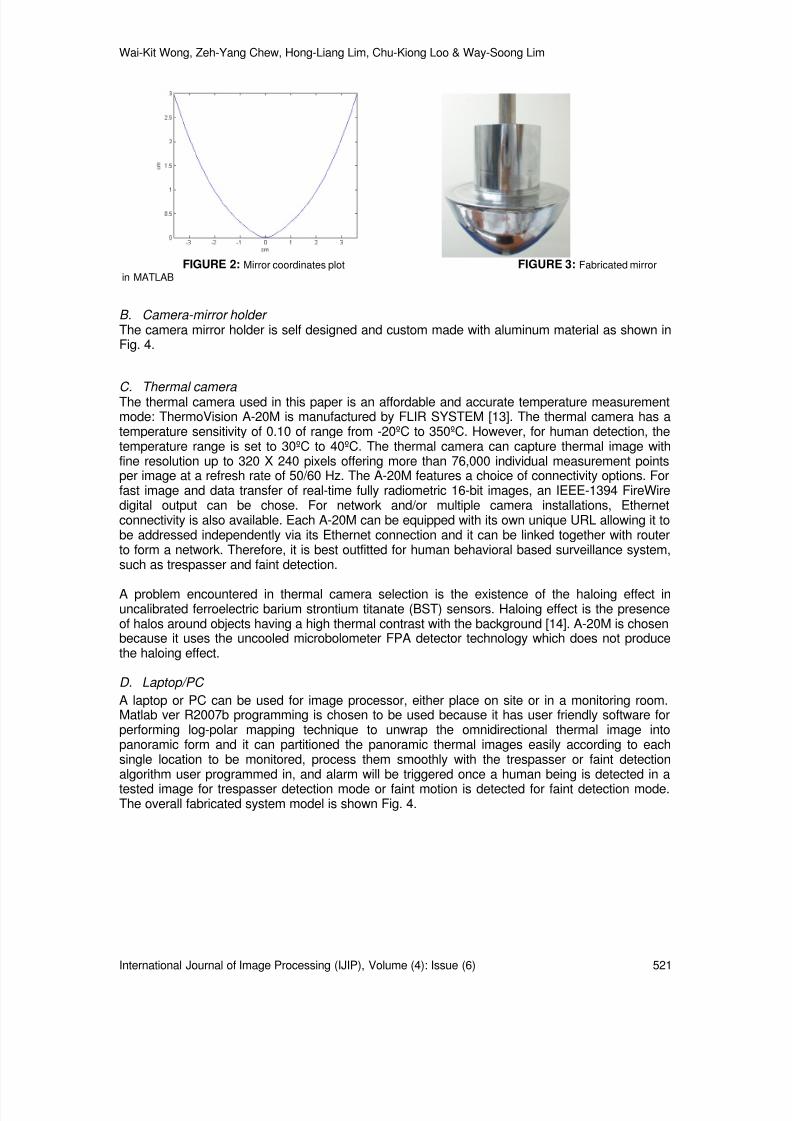
mirror dimension. The first parameter is the focal length of the camera f , in which for the thermalcamera in use is 12.5 mm and the distance d ( ρz -plane) from the origin is set to 2 m. The imageplane height h is set to 20 cm. the radius of the mirror rim is chosen t 1=3.6cm as modified fromSvoboda work in [12], with radius for fovea region 0.6 cm and retina region 3.0 cm. Fovea angleis set in between 0º to 45º, whereas retina angle is from 45º to 135º. The coordinates as well asthe plot of the mirror shape is generated using MATLAB and shown in Fig. 2. The coordinates aswell as mechanical drawing using Autocad are provided to precision engineering company tofabricate/custom made the hyperbolic mirror. The hyperbolic mirror is milling by using aluminumbar and then chrome plating with a chemical element named chromium. Chromium is regardedwith great interest because of its lustrous (good in IR reflection), high corrosion resistance, highmelting point and hardness. The fabricated mirror is shown in Fig. 3.
8/6/2019 International Journal of Image Processing (IJIP) Volume 4 Issue 6
http://slidepdf.com/reader/full/international-journal-of-image-processing-ijip-volume-4-issue-6 12/172
Wai-Kit Wong, Zeh-Yang Chew, Hong-Liang Lim, Chu-Kiong Loo & Way-Soong Lim
International Journal of Image Processing (IJIP), Volume (4): Issue (6) 521
FIGURE 2: Mirror coordinates plot FIGURE 3: Fabricated mirrorin MATLAB
B. Camera-mirror holder The camera mirror holder is self designed and custom made with aluminum material as shown inFig. 4.
C. Thermal camera The thermal camera used in this paper is an affordable and accurate temperature measurementmode: ThermoVision A-20M is manufactured by FLIR SYSTEM [13]. The thermal camera has atemperature sensitivity of 0.10 of range from -20ºC to 350ºC. However, for human detection, thetemperature range is set to 30ºC to 40ºC. The thermal camera can capture thermal image withfine resolution up to 320 X 240 pixels offering more than 76,000 individual measurement pointsper image at a refresh rate of 50/60 Hz. The A-20M features a choice of connectivity options. Forfast image and data transfer of real-time fully radiometric 16-bit images, an IEEE-1394 FireWiredigital output can be chose. For network and/or multiple camera installations, Ethernetconnectivity is also available. Each A-20M can be equipped with its own unique URL allowing it tobe addressed independently via its Ethernet connection and it can be linked together with routerto form a network. Therefore, it is best outfitted for human behavioral based surveillance system,such as trespasser and faint detection.
A problem encountered in thermal camera selection is the existence of the haloing effect inuncalibrated ferroelectric barium strontium titanate (BST) sensors. Haloing effect is the presenceof halos around objects having a high thermal contrast with the background [14]. A-20M is chosenbecause it uses the uncooled microbolometer FPA detector technology which does not producethe haloing effect.
D. Laptop/PC A laptop or PC can be used for image processor, either place on site or in a monitoring room.Matlab ver R2007b programming is chosen to be used because it has user friendly software forperforming log-polar mapping technique to unwrap the omnidirectional thermal image intopanoramic form and it can partitioned the panoramic thermal images easily according to eachsingle location to be monitored, process them smoothly with the trespasser or faint detectionalgorithm user programmed in, and alarm will be triggered once a human being is detected in atested image for trespasser detection mode or faint motion is detected for faint detection mode.The overall fabricated system model is shown Fig. 4.

8/6/2019 International Journal of Image Processing (IJIP) Volume 4 Issue 6
http://slidepdf.com/reader/full/international-journal-of-image-processing-ijip-volume-4-issue-6 13/172
Wai-Kit Wong, Zeh-Yang Chew, Hong-Liang Lim, Chu-Kiong Loo & Way-Soong Lim
International Journal of Image Processing (IJIP), Volume (4): Issue (6) 522
FIGURE 4: Overall fabricated omnidirectional thermal imaging surveillance system model
3. LOG-POLAR MAPPINGIn this section, log-polar mapping is proposed for unwarping the captured omnidirectional thermalimages into panoramic form providing the observer or image processing tools a complete wideangle of view. Log-polar geometry or log-polar transform in short, is an example of foveated orspace-variant image representation used in the active vision systems motivated by human visualsystem [15]. It is a spatially-variant image representation in which pixel separation increaseslinearly with distance from a central point [16]. It provides a way of concentrating computationalresources on regions of interest, whilst retaining low-resolution information from a wider field of
view. One advantage of this kind of sampling is data reduction. Foveal image representations likethis are most useful in the context of active vision system where the densely sampled centralregion can be directed to pick up the most salient information. Human eyes are very roughlyorganized in this way.
In robotics, there has been a trend to design and use true retina-like sensors [17], [18] or simulatethe log-polar images by software conversion [19], [20]. In the software conversion of log-polarimages, practitioners in pattern recognition usually named it as log-polar mapping. Theadvantages of log-polar mapping is that it can unwarp an omnidirectional image into panoramicimage, hence providing the observer and image processing tools a complete wide angle of viewfor the surveillance area’s surroundings and preserving fine output image quality in a higher datacompression manner. The spatially-variant grid that represents log-polar mapping is formed by i number of concentric circles with N samples over each concentric circle [15]. An example of aspatially-variant sampling grid is shown in Fig. 5.
The log-polar mapping use in this paper can be summarized as following: Initially, omnidirectionalthermal image is captured using a thermal camera and a custom made IR reflected hyperbolicmirror. The geometry of the captured omnidirectional thermal image is in Cartesian form (x 1,y1).Next, the Cartesian omnidirectional thermal image is sampled by the spatially-variant grid into alog-polar form ( ρ,θ ) omnidirectional thermal image. After that, the log-polar omnidirectionalthermal image is unwarped into a panoramic thermal image (x 2,y2), another Cartesian form. Sincethe panoramic thermal image is in Cartesian form, subsequent image processing task willbecome much easier.

8/6/2019 International Journal of Image Processing (IJIP) Volume 4 Issue 6
http://slidepdf.com/reader/full/international-journal-of-image-processing-ijip-volume-4-issue-6 14/172
Wai-Kit Wong, Zeh-Yang Chew, Hong-Liang Lim, Chu-Kiong Loo & Way-Soong Lim
International Journal of Image Processing (IJIP), Volume (4): Issue (6) 523
The center of pixel for log-polar sampling is described by [15]:
) ρ R
(ln) ρ( bο
=11 y,x (1)
)(π
N )θ (
1
1111 x
ytan
2y,x −
= (2)
The center of pixel for log-polar mapping is described as:
) N
)πθ (( ρ 11
2
y,x2cos),(x =θ ρ (3)
) N
)πθ (( ρ 11
2
y,x2sin),(y =θ ρ (4)
where R is the distance between given point and the center of mapping = 21
21 y x + ,
ρο is the scaling factor which will define the size of the circle at ρ(x1,y1) = 0,b is the base of the algorithm [15],
π N π N
b−
+= (5)
N is the number of angular samples over each concentric circle.
FIGURE 7: A graphical view of log-polar mapping.
A graphical view illustrating the log-polar mapping is shown in Fig. 5 [15]. To sample theCartesian pixels (x 1,y1) into log-polar pixel ( ρ,θ ), at each center point calculated using (1) and (2),the corresponding log-polar pixel ( ρn ,θ n ) covers a region of Cartesian pixels with radius:
1nn −= br r (6)
where n = 1,2,3,….., N -1. Fig. 6 shows the circle sampling method of log-polar mapping [15], [21],where A, A’, B and B’ points are the centre of pixel for log-polar sampling.
8/6/2019 International Journal of Image Processing (IJIP) Volume 4 Issue 6
http://slidepdf.com/reader/full/international-journal-of-image-processing-ijip-volume-4-issue-6 15/172
Wai-Kit Wong, Zeh-Yang Chew, Hong-Liang Lim, Chu-Kiong Loo & Way-Soong Lim
International Journal of Image Processing (IJIP), Volume (4): Issue (6) 524
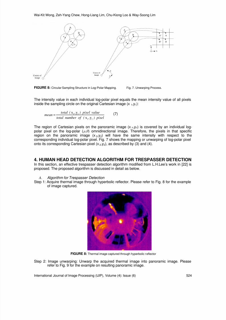
FIGURE 8: Circular Sampling Structure in Log-Polar Mapping. Fig. 7. Unwarping Process.
The intensity value in each individual log-polar pixel equals the mean intensity value of all pixelsinside the sampling circle on the original Cartesian image (x 1,y1):
pixel)(of number totalvalue pixel)(totalmean11
11
y,xy,x= (7)
The region of Cartesian pixels on the panoramic image (x 2,y2) is covered by an individual log-polar pixel on the log-polar ( ρ,θ ) omnidirectional image. Therefore, the pixels in that specificregion on the panoramic image (x 2,y2) will have the same intensity with respect to thecorresponding individual log-polar pixel. Fig. 7 shows the mapping or unwarping of log-polar pixelonto its corresponding Cartesian pixel (x 2,y2), as described by (3) and (4).
4. HUMAN HEAD DETECTION ALGORITHM FOR TRESPASSER DETECTIONIn this section, an effective trespasser detection algorithm modified from L.H.Lee’s work in [22] isproposed. The proposed algorithm is discussed in detail as below.
A. Algorithm for Trespasser Detection Step 1: Acquire thermal image through hyperbolic reflector. Please refer to Fig. 8 for the example
of image captured.
FIGURE 8: Thermal image captured through hyperbolic reflector
Step 2: Image unwarping: Unwarp the acquired thermal image into panoramic image. Pleaserefer to Fig. 9 for the example on resulting panoramic image.
8/6/2019 International Journal of Image Processing (IJIP) Volume 4 Issue 6
http://slidepdf.com/reader/full/international-journal-of-image-processing-ijip-volume-4-issue-6 16/172
Wai-Kit Wong, Zeh-Yang Chew, Hong-Liang Lim, Chu-Kiong Loo & Way-Soong Lim
International Journal of Image Processing (IJIP), Volume (4): Issue (6) 525
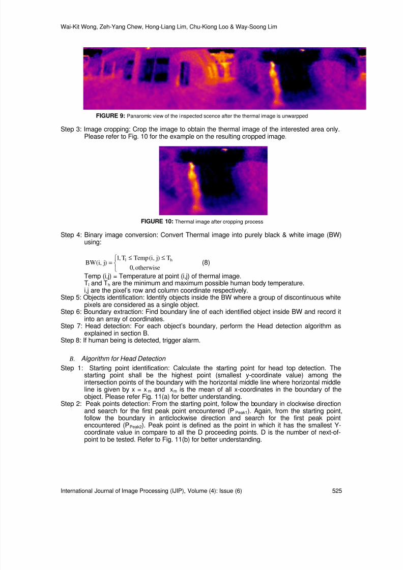
FIGURE 9: Panaromic view of the inspected scence after the thermal image is unwarpped
Step 3: Image cropping: Crop the image to obtain the thermal image of the interested area only.Please refer to Fig. 10 for the example on the resulting cropped image.
FIGURE 10: Thermal image after cropping process
Step 4: Binary image conversion: Convert Thermal image into purely black & white image (BW)using:
≤≤=
otherwise,0
T) j,i(TempT,1) j,i(BW hl (8)
Temp (i,j) = Temperature at point (i,j) of thermal image.Tl and T h are the minimum and maximum possible human body temperature.i,j are the pixel’s row and column coordinate respectively.
Step 5: Objects identification: Identify objects inside the BW where a group of discontinuous whitepixels are considered as a single object.Step 6: Boundary extraction: Find boundary line of each identified object inside BW and record it
into an array of coordinates.Step 7: Head detection: For each object’s boundary, perform the Head detection algorithm as
explained in section B.Step 8: If human being is detected, trigger alarm.
B. Algorithm for Head Detection Step 1: Starting point identification: Calculate the starting point for head top detection. The
starting point shall be the highest point (smallest y-coordinate value) among theintersection points of the boundary with the horizontal middle line where horizontal middleline is given by x = x m and x m is the mean of all x-coordinates in the boundary of the
object. Please refer Fig. 11(a) for better understanding.Step 2: Peak points detection: From the starting point, follow the boundary in clockwise directionand search for the first peak point encountered (P Peak1 ). Again, from the starting point,follow the boundary in anticlockwise direction and search for the first peak pointencountered (P Peak2 ). Peak point is defined as the point in which it has the smallest Y-coordinate value in compare to all the D proceeding points. D is the number of next-of-point to be tested. Refer to Fig. 11(b) for better understanding.

8/6/2019 International Journal of Image Processing (IJIP) Volume 4 Issue 6
http://slidepdf.com/reader/full/international-journal-of-image-processing-ijip-volume-4-issue-6 17/172
Wai-Kit Wong, Zeh-Yang Chew, Hong-Liang Lim, Chu-Kiong Loo & Way-Soong Lim
International Journal of Image Processing (IJIP), Volume (4): Issue (6) 526
(a) (b)
FIGURE 11: (a)Horizontal middle line and the starting point as in step1. (b) Detection of (c/w from Startingpoint) and (couter c/w from starting point)
Step 3: Head top point detection: Compare P Peak1 and P Peak2 obtained in step 2. Record the
highest point (with smaller Y-coordinate) as the head top point, P HT. For example, in Fig.11(b), P Peak2 is higher thanP Peak1 . Thus P HT = P Peak2 .Step 4: Boundary line splitting: Split the boundary into left boundary (Bl) and right boundary (Br)
from the head top point towards bottom. Take only one point for each y-coordinate tofilter out unwanted information such as raised hands. (Refer Fig. 12 for betterunderstanding).
(a) (b)
FIGURE 12: a) Original object boundary. (b) Left and Right object boundary after the splitting process (step4).
Bl=[xli,yli] , Br=[xr i,yr i] (9)Where xl i,yli,xr i,yr i are the pixels’ y-coordinates and x-coordinates for left boundary andright boundary respectively.
I=1…N is the index number.N=size of the boundary matrix (N is the number of pixels for left and rightboundary)
Step 5: Left significant points detection: Search downwards along left boundary (Bl) from P HT forthe first leftmost point encountered (Pl p). Next, search for the rightmost point right afterPl p which is Pl d. Refer Fig. 13 for better understanding.
Pl p=(xl lp, yl lp), Pl d=(xlld, ylld) (10)Where subscript lp = index number of the first leftmost point

8/6/2019 International Journal of Image Processing (IJIP) Volume 4 Issue 6
http://slidepdf.com/reader/full/international-journal-of-image-processing-ijip-volume-4-issue-6 18/172
Wai-Kit Wong, Zeh-Yang Chew, Hong-Liang Lim, Chu-Kiong Loo & Way-Soong Lim
International Journal of Image Processing (IJIP), Volume (4): Issue (6) 527
Subscript ld = index number of the rightmost point right after Pl p
Step 6: Right significant points detection: Search downwards along right boundary (Br) from P HT for the first rightmost point encountered (Pr p). Next, detect the leftmost point right afterPr p which is Pr d. Refer Fig. 6 for better understanding.
Pr p=(xr rp, yr rp), Pr d=(xr rd, yr rd) (11)Where subscript rp = index number of the first rightmost point
subscript rd = index number of the first leftmost point right after Pr p
FIGURE 13: Example of points found in step 3, step 5 and step 6.
Step 7: Head symmetric test:Define h l = Vertical distance between P HT and Pl d
hr = Vertical distance between P HT and Pr d Test the ratio between h l and h r. If h l /h r or h r /h l > 2, then this object is not considered as ahuman being and we can skip the next subsequent steps in this algorithm and proceedwith the next object. Else, the object has the possibility to be considered as a humanbeing. Continue step 8 for further detection.
Step 8: Neck-body position test: Calculate ∆x, which is the distance between x c and x m where x c =horizontal center between Pl d and Pr d and x m is obtained in step1. Define w n =horizontal distance between Pl d and Pr d.If ∆x ≥ 2wn, then this object is not considered as a human being and we can skip the nextsubsequent steps in this algorithm and proceed with next object. Else if ∆x < 2w n , thenthe object has the possibility to be considered as a human being. Continue step 9 forfurther detection.
Step 9: Curve tests:
I) TOP CURVE TEST .Define s t=floor(min(lp,rp)/(F/2)) as the step size for top curve test.Calculate:
≤=
+++
otherwise,0
ylyl,1C )1k (*s1k *s1
tltt
≤
=+++
otherwise,0
yryr,1C
)1k (*s1k *s1tr tt (12)
C t = ∑ C tl + ∑ Ctr
where k=0, …,F/2-1F is the step size partition variable. F is even integer and F ≥2.
For example, if F=6,s t=8, then the y-coordinates tested is as shown in Fig. 14. Thesame concept goes for left curve test and right curve test.Note: the symbol ‘*’ means multiply.

8/6/2019 International Journal of Image Processing (IJIP) Volume 4 Issue 6
http://slidepdf.com/reader/full/international-journal-of-image-processing-ijip-volume-4-issue-6 19/172
Wai-Kit Wong, Zeh-Yang Chew, Hong-Liang Lim, Chu-Kiong Loo & Way-Soong Lim
International Journal of Image Processing (IJIP), Volume (4): Issue (6) 528
FIGURE 14: Example on top curve test.
II) LEFT CURVE TEST Define s l = floor(min(lp,ld-lp)/(F/2)) as the step size for left curve test.Calculate:
≤=
+++
otherwise,0
xlxl,1C )1k (*slpk *slp
1lll
≤=
+−−
otherwise,0
xlxl,1C )1k (*slpk *slp
2lll (13)
C l = ∑C l1 + ∑C l2 where k=0, …,F/2-1
III) RIGHT CURVE TEST Define s r = floor(min(rp,rd-rp)/(F/2)) as the step size for right curve test.Calculate:
≥=
+++
otherwise,0
xrxr,1C )1k (*srpk *srp
1rrr
≥=
+−−
otherwise,0
xrxr,1C )1k (*srpk *srp
2rrr (14)
C r = ∑C r1 + ∑C r2
Where k=0, …,F/2-1Step 10: Human identification:
Define curve test condition:C t ≥ F-1 - (15)C l ≥ F-1 - (16)C r ≥ F-1 - (17) Check condition (15),(16) and (17). If any two or more conditions are true, the object isverified as a human being. Else, the object is not considered as a human being.
5. HOME ALONE FAINT DETECTION ALGORITHM In this section, an effective faint detection algorithm for monitoring home alone personal isproposed for the omnidirectional thermal imaging surveillance system.
Step 1: Global parameters definition: Define global parameters to be used in the designedalgorithm such as H p = human’s height in previous image, H c = human’s height in currentimage, W p = human’s width in previous image and W c = human’s width in current image, f = accumulator for human lying image, F = total frames (time) to decide whether a humanbeing is fainted, S = smallest possible human being’s size (in terms of number of pixels ingroup) in an image, H max = maximum height of human of image being capture andinitialize it to 0.
Step 2: Image acquisition: Acquire image of background image from thermal camera, unwarp itand store as RGB image, B . Acquire image from thermal camera, unwarp it and store asRGB image, I . An example of B and I is shown in Fig 15.

8/6/2019 International Journal of Image Processing (IJIP) Volume 4 Issue 6
http://slidepdf.com/reader/full/international-journal-of-image-processing-ijip-volume-4-issue-6 20/172
Wai-Kit Wong, Zeh-Yang Chew, Hong-Liang Lim, Chu-Kiong Loo & Way-Soong Lim
International Journal of Image Processing (IJIP), Volume (4): Issue (6) 529
(a)
(b)
FIGURE 15: Thermal image capture on site corresponding (a) Example of B (b) Example of I
Step 3: Background subtraction: Subtract image B from image I and store it as image, Im. Step 4: Binary image conversion:
a) Convert Im to gray scale image, G . An example of G shown in Fig 16b) Convert G to binary image, B 1 using minimum possible human body temperature
threshold, T . An example of B 1 shown in Fig 17.Step 5: Noise Filtering:
a) Removes from B 1 all connected components (objects) that have fewer than S pixels,producing another binary image, B 2 . An example of B 2 is shown in Fig. 18.
b) Creates a flat, disk-shaped structuring element, SE with radius, R . An example ofstructuring element is shown in Fig. 19.c) Performs morphological closing on the B 2 , returning a closed image , B 3 . Morphological
definition for this operation is dilates an image and then erodes the dilated image usingthe same SE for both operations. An example of B 3 shown in Fig. 20.
d) Perform Hole Filling in B 3 and returning a filled image A: A hole may be defined as abackground region surrounded by a connected border of foreground pixels. Anexample of A shown in Fig. 21.
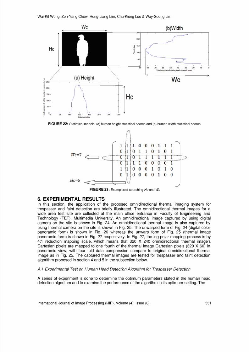
Step 6: Human’s height statistical search: Summing each pixels contents in every single columnof A to form a statistical model as shown in Fig 22(a). From the statistical model, searchfor H c (the highest value in the plot). An example of searching H c is shown in Fig 23.
Step 7: Human’s width statistical search: Summing each pixels contents in every single rows of A to form a statistical model as shown in Fig 22(b). From the statistical model,search for W c (the highest value in the plot). An example of searching W c is shown in Fig
23.Step 8: If H c >H max , set H c =H max .Step 9: Faint detection:
IF H c ≥ W c and H c ≥ (95% of H max )THEN the human is considered standing or walking. Continue on step 10.
IF H c ≥ W c and Hc< (95% of H max )THEN the human is considered fall down. Continue on step 10.
IF H c < W c and W c ≠W p and/or H c ≠H p and f < F ,THEN the human is fall down. Continue on step 10.
IF H c < W c and W c =W p and H c =H p and f < F ,THEN the human is considered possible faint. Continue on step 11.
IF H c <W c and W c =W p and H c =H p and f ≥ F ,THEN the human is considered faint. Continue on step 12.
Step 10: Reset fainted frame counter and start new cycle: Set f = 0, update H p = H c and W p = W c .
Repeat step 2.Step 11: Increase frame counter by 1 and start new cycle: Set f = f + 1, update H p =H c and W p = W c . Repeat step 2.
Step 12: Faint case: Signals alarm until operator noted and performs rescue action and resets thesystem manually.

8/6/2019 International Journal of Image Processing (IJIP) Volume 4 Issue 6
http://slidepdf.com/reader/full/international-journal-of-image-processing-ijip-volume-4-issue-6 21/172
Wai-Kit Wong, Zeh-Yang Chew, Hong-Liang Lim, Chu-Kiong Loo & Way-Soong Lim
International Journal of Image Processing (IJIP), Volume (4): Issue (6) 530
FIGURE 16: Example of image G
FIGURE 17: Example of image B1
FIGURE 18: Example of image B2
FIGURE 19: Disk shaped structuring elements
FIGURE 20: Example of image B3
FIGURE 21: Example of image A
8/6/2019 International Journal of Image Processing (IJIP) Volume 4 Issue 6
http://slidepdf.com/reader/full/international-journal-of-image-processing-ijip-volume-4-issue-6 22/172
Wai-Kit Wong, Zeh-Yang Chew, Hong-Liang Lim, Chu-Kiong Loo & Way-Soong Lim
International Journal of Image Processing (IJIP), Volume (4): Issue (6) 531
FIGURE 22: Statistical models: (a) human height statistical search and (b) human width statistical search.
FIGURE 23: Examples of searching Hc and Wc
6. EXPERIMENTAL RESULTSIn this section, the application of the proposed omnidirectional thermal imaging system fortrespasser and faint detection are briefly illustrated. The omnidirectional thermal images for awide area test site are collected at the main office entrance in Faculty of Engineering andTechnology (FET), Multimedia University. An omnidirectional image captured by using digitalcamera on the site is shown in Fig. 24. An omnidirectional thermal image is also captured byusing thermal camera on the site is shown in Fig. 25. The unwarped form of Fig. 24 (digital colorpanoramic form) is shown in Fig. 26 whereas the unwarp form of Fig. 25 (thermal imagepanoramic form) is shown in Fig. 27 respectively. In Fig. 27, the log-polar mapping process is by4:1 reduction mapping scale, which means that 320 X 240 omnidirectional thermal image’s
Cartesian pixels are mapped to one fourth of the thermal image Cartesian pixels (320 X 60) inpanoramic view, with four fold data compression compare to original omnidirectional thermalimage as in Fig. 25. The captured thermal images are tested for trespasser and faint detectionalgorithm proposed in section 4 and 5 in the subsection below.
A.) Experimental Test on Human Head Detection Algorithm for Trespasser Detection
A series of experiment is done to determine the optimum parameters stated in the human headdetection algorithm and to examine the performance of the algorithm in its optimum setting. The

8/6/2019 International Journal of Image Processing (IJIP) Volume 4 Issue 6
http://slidepdf.com/reader/full/international-journal-of-image-processing-ijip-volume-4-issue-6 23/172
Wai-Kit Wong, Zeh-Yang Chew, Hong-Liang Lim, Chu-Kiong Loo & Way-Soong Lim
International Journal of Image Processing (IJIP), Volume (4): Issue (6) 532
FIGURE 24: Case studies of trespasser and faint detection captured at main office entrance in FET (digitalcolor form).
FIGURE 25: Case studies of trespasser and faint detection captured at main office entrance in FET (thermalimage).
FIGURE 26: Unwarp form of Fig. 24 (digital color panoramic form)
FIGURE 27: Unwarp form of Fig. 25 (thermal image panoramic form)

8/6/2019 International Journal of Image Processing (IJIP) Volume 4 Issue 6
http://slidepdf.com/reader/full/international-journal-of-image-processing-ijip-volume-4-issue-6 24/172
Wai-Kit Wong, Zeh-Yang Chew, Hong-Liang Lim, Chu-Kiong Loo & Way-Soong Lim
International Journal of Image Processing (IJIP), Volume (4): Issue (6) 533
testing site is the main office entrance of Faculty of Engineering and Technology, MultimediaUniversity, which simulates the door of a nursing home, for tracking Alzheimer patients fromleaving nursing home without permission and theft during night time. The omnidirectional thermalimaging tool is setup with the height of 1.5m. This setting is chosen because it gives the best viewof the testing site. A total of 10,000 thermal images with test subjects (human being or animal)roaming randomly in the area visible to the proposed system are taken.To determine optimum value for parameter T l, a random sample image is chosen and convertedinto B&W image using step 2 of the Algorithm for Trespasser Detection with value of T l rangingfrom 0 to 510 (sum of R and G component in RGB image. B component is excluded because it isnot proportional to the change of temperature). Perform the binary image conversion repeatedlywith increasing step size of 10 for T l and search for the optimum T l where the noise can beminimized and the human is not distorted in the resulting image. The optimum setting found for T l is 150 in this experiment. For example, if T l =130 is used, excessive noise will be introduced. If T l =170 is used, there will be too much distortion to human being in the resulting image. Refer Fig.28 for better understanding.
(a) (b) (c)
FIGURE 28: (a) T l =130 (b) T l =150 (c) T l =170.
To determine the optimum value for parameter T h, perform the binary image conversionrepeatedly with decreasing step size of 10 for T h and search for the minimum value of T h whichdoes not influence the appearance of the human object. The optimum value found for T h is 430 inthis experiment. For example, if T h =400 is used, the image of human being is distorted. If T h =460 is used, there will be no improvement for the image. Lower T h value is preferred because itwill filter out more high temperature noise component. Refer Fig. 29 for better understanding.
(a) (b) (c)
FIGURE 29: (a) T h =400 (b) T h =430 (c) T h =460.
The accuracy of the proposed algorithm is then evaluated using ‘operator perceived activity’(OPA) in which the proposed algorithm is evaluated with respect with the results interpreted by ahuman observer [7],[23]. Firstly, the thermal images are tested using the proposed algorithm.Then, the result is compared with the result of the human observer. The accuracy of the proposedalgorithm is the percentage of interpretation (trespasser or not) agreed by both the humanobserver and the proposed algorithm.

8/6/2019 International Journal of Image Processing (IJIP) Volume 4 Issue 6
http://slidepdf.com/reader/full/international-journal-of-image-processing-ijip-volume-4-issue-6 25/172
Wai-Kit Wong, Zeh-Yang Chew, Hong-Liang Lim, Chu-Kiong Loo & Way-Soong Lim
International Journal of Image Processing (IJIP), Volume (4): Issue (6) 534
FIGURE 30: Accuracy of proposed algorithm for diff erent combination of D and F.
To determine parameter D and F, all of the 10,000 images in group 1 are tested with differentcombinations of D and F. As shown in the graph in Fig. 30, the optimum value for parameter D
and F are 7 and 2 which contribute to accuracy of 81.38%. From the observation, the smallest thestep size partition variable (F), the accurate the trespasser detection is. D is optimum at 7proceeding points, more than 7 proceeding points or lesser will degrade the overall performanceof the trespasser detection accuracy. The proposed algorithm is able to operate in a very fastmanner whereby the routine time required to capture a thermal image, unwarped into panoramicform, detect the existence of a trespasser and trigger the alarm is only 2.27 seconds.
B.) Experimental Test on Home Alone Faint Detection
In this section, the proposed algorithm for faint detection will be briefly discussed. The testing siteis at the lobby around the main entrance of the Faculty of Engineering and Technology,Multimedia University, which simulates the activities area of a nursing home/hospital. Forexperimental purpose, 17,878 sample images include background image had been captured totest the accuracy of the proposed faint detection algorithm. At the test site, omnidirectionalthermal images had been captured using the omnidirectional thermal imaging system, unwarpedinto panoramic form, performed image filtering, image processing for faint detection and signalalarm or not. These images included different poses of human such as standing or walking, falling,and fainting. The system routine time including the time for capture in omnidirectional thermalimage, unwarping into panoramic form, image filtering, faint detection and signal alarm or not is 1frame per second. Thus F as an example is set to 7 so that if a person lies on the same placewith same size for 7 second, the system will classify the person is fainting.
The thermal image temperature range has been set from 25°C to 38°C. Human shape’sparameters S and R are approximate from one of the testing image at a distance of 5 meters fromthe imaging system. From that image, the human’s total pixels are only 30. Hence, S is set to 30and R for SE is set to 2 respectively. Then, different T are tried in order to get the approximatehuman shape. T found to be falls within the range of 100 to 126. The T value depends on thetemperature of the environment. At night time, T value is about 120 to 126, whereas in theafternoon, the T value is about 100 to 120.
Some example images of different human poses are shown in Fig. 31-33 (each for standing,falling (bending body) and fainting respectively). To differentiate between human standing motionand human bending body motion, a parameter, p has been set according to the factor of Hmax .The p value are found achieved highest accuracy when p = 95% of Hmax from Fig 6.14. Hence p value was set to 95% of Hmax . The proposed algorithm had been tested at night time with poorlighting condition at outdoor. The table I show the accuracies of the proposed faint detectionalgorithm on site.

8/6/2019 International Journal of Image Processing (IJIP) Volume 4 Issue 6
http://slidepdf.com/reader/full/international-journal-of-image-processing-ijip-volume-4-issue-6 26/172
Wai-Kit Wong, Zeh-Yang Chew, Hong-Liang Lim, Chu-Kiong Loo & Way-Soong Lim
International Journal of Image Processing (IJIP), Volume (4): Issue (6) 535
(a)
(b)FIGURE 31: Standing motion (a) Thermal image (b) Black and white image
(a)
(b)FIGURE 32: Falling/bending body motion (a) Thermal image (b) Black and white image
(a)
(b)FIGURE 33: Fainting motion (a) Thermal image (b) Black and white image

8/6/2019 International Journal of Image Processing (IJIP) Volume 4 Issue 6
http://slidepdf.com/reader/full/international-journal-of-image-processing-ijip-volume-4-issue-6 27/172
Wai-Kit Wong, Zeh-Yang Chew, Hong-Liang Lim, Chu-Kiong Loo & Way-Soong Lim
International Journal of Image Processing (IJIP), Volume (4): Issue (6) 536
Fig. 34: Graph of accuracy versus p
Motion Testframes
Success Fail Accuracy(%)
Standing ,walking
6550 6498 52 99.20
Falling 4578 3983 595 86.78Fainting 6750 6043 707 89.50Total 17878 16524 1354 92.42
TABLE I. OUTDOOR MOTION DETECTION AT NIGHT W ITH P OOR AMBIENT LIGHT C ONDITION
The results in table I show that standing or walking motion has highest accuracy compare tofalling and fainting motion with 99.20%. The reason that falling motion has the lowest accuracy(with 86.78%) is because some of the falling motion is considered as standing motion in theproposed system. Besides, 89.5% of the fainting motion was detected correctly among the totaltested images. Lastly, the proposed algorithm was well performed on poor lighting conditions atnight with an average accuracy of 92.42%. Overall, the system can classify human behavioralbest in normal standing or walking motion and good in detecting fainting motion as well no matterin good or poor lighting condition. The home alone faint detection surveillance system alsofunctions in a fast way whereby the routine time required to capture in a thermal image, unwarpinto panoramic form, detect whether there is a faint suspected case until the signal alarm or not isonly 1.85 seconds. When there is a fainting motion detected, the alarm will be trigger until theoperator performs the rescue action and resets the system manually.
7. CONCLUSIONIn this paper, the usage of hyperbolic IR reflected mirror is proposed in a thermal imaging systemfor omnidirectional thermal imaging smart surveillance purposes In the proposed system, bothhuman detection and faint detection algorithm has been implemented in order to facilitate smartsurveillance functionality which is able to greatly increase the effectiveness of the surveillancesystem. The trespasser detection algorithm is used mainly to detect unauthorized movement toand fro the building while the faint detection algorithm is used to detect the event where humanbeing faint inside the premise.
For human head detection algorithm, the thermal images are first converted into binary (Blackand White) images. The presence of human being is then analyzed based on the shape of theobjects (head detection) in the binary image. From the experimental results, it is shown that theproposed trespasser detection algorithm is able to achieve an accuracy of 81.38% with a routinetime of 2.27 seconds. For home alone faint detection algorithm, it enables the faint event to bedetected even in poor lighting condition. The experimental results show that the proposed faintdetection algorithm in the omnidirectional surveillance system achieved high accuracy inmonitoring the faint event in the poor lighting condition with the accuracy of 89.50% with a routinetime of 1.85 seconds.
There are some distortion on the captured thermal image whereby the temperature surroundingwill affect the accuracy for both the proposed trespasser and faint detection algorithm. Forexample, the temperature surrounding which is nearly equal to the human body will make thehuman body undistinguishable from the temperature surrounding. Besides, the clothes of thehuman with lower temperature (human sweating) will causes part of the actual human bodytemperature changed.
In future, a plan is proposed to combine visible/infrared image fusion model into the currentlyproposed model to improve the performance of the trespasser and faint detection. In additional tothat, it is also planning to employ microprocessor modules such as FPGA (field programmablegate array) and ARM (Advanced RISC Machine) for the image processing and analyzing tasksinstead of a computer to effectively reduce the costs and power consumption of the proposedsystem. These topics will be addressed in future works.

8/6/2019 International Journal of Image Processing (IJIP) Volume 4 Issue 6
http://slidepdf.com/reader/full/international-journal-of-image-processing-ijip-volume-4-issue-6 28/172
Wai-Kit Wong, Zeh-Yang Chew, Hong-Liang Lim, Chu-Kiong Loo & Way-Soong Lim
International Journal of Image Processing (IJIP), Volume (4): Issue (6) 537
8. REFERENCES[1] A. Hampapur, L. Brown, J. Connell, S. Pankanti, A. Senior et al., “Smart Surveillance:
Applications, Technologies and Implications”, Information, Communications and SignalProcessing, Vol. 2, p.p. 1133-1138.
[2] A. Hampapur, L. Brown, J. Connell, A. Ekin, N. Haas, M. Lu et al., “Smart Video Surveillance”,
IEEE Signal Processing Mag., March 2005, p.p. 39-51.
[3] M.W. Green, “The appropriate and effective use of security technologies in U.S. schools, Aguide for schools and law enforcement agencies”, Sandia National Laboratories, Albuquerque,NM, NCJ 178265, Sep 1999.
[4] C. Shu, A. Hampapur, M. Lu, L. Brown, J. Connell et al., “IBM Smart Surveillance System(S3): A Open and Extensible Framework for Event Based Surveillance”, in Advanced Videoand Signal Based Surveillance (AVSS 2005), 2005, p.p. 318-323.
[5] C. Lu, and M. S. Drew, “Automatic Compensation for Camera Settings for ImagesTakenUnder Different Illuminants”, Technical paper, School of Computer Science, Simon FraserUniversity, Vancouver, British Columbia, Canada, 2007, p.p. 1-5.
[6] Thermographic camera. Retrieved from Wikipedia, the free encyclopedia Web Site:http://en.wikipedia.org/wiki/Thermal_camera .
[7] W.K. Wong, P.N. Tan, C.K. Loo and W.S. Lim, “An Effective Surveillance System UsingThermal Camera”, 2009 International Conference on Signal Acquisition and Processing(ICSAP2009) 3-5 Apr, 2009, Kuala Lumpur, Malaysia, p.p. 13-17.
[8] M.R. Narayanan, S.R. Lord, M.M. Budge, B.G. Cellar and N.H. Novell, “Falls Management:Detection and Prevention, using a Waist-mounted Triaxial Accelerometer”, 29 th AnnualInternational Conference of the IEEE Engineering in Medicine and Biology Society, 2007,p.p.4037-4040.
[9] J. Han and B. Bhanu, “Fusion of color and infrared video for moving human detection”, ACMPortal, Pattern Recognition, p.p. 1771-1784.
[10] J. Chahl and M. Srinivasan, “Reflective surfaces for panoramic imaging”, Applied Optics ,36(31), Nov 1997, p.p.8275-85.
[11] S. Gachter, “Mirror Design for an Omnidirectional Camera with a Uniform CylindricalProjection when Using the SVAVISCA Sensor”, Research Reports of CMP, OMNIVIEWSProject, Czech Technical University in Prague, No. 3, 2001. Redirected from:http://cmp.felk.cvut.cz/projects/omniviews/
[12] T. Svoboda, Central Panoramic Cameras Design, Geometry, Egomotion. PhD Theses,Center of Machine Perception, Czech Technical University in Prague, 1999.
[13] http://www.flirthemography.com
[14] J.W. Davis and V. Sharma, “Background-Subtraction in Thermal Imagery Using ContourSaliency”, International Journal of Computer Vision 71(2), 2007, p.p. 161-181.
[15] H. Araujo, J. M. Dias, “An Introduction To The Log-polar Mapping”, Proceedings of 2nd Workshop on Cybernetic Vision , 1996, p.p. 139-144.
[16] C. F. R. Weiman and G. Chaikin, “Logarithmic Spiral Grids For Image Processing AndDisplay”, Computer Graphics and Image Processing , Vol. 11, 1979, p.p. 197-226.

8/6/2019 International Journal of Image Processing (IJIP) Volume 4 Issue 6
http://slidepdf.com/reader/full/international-journal-of-image-processing-ijip-volume-4-issue-6 29/172
Wai-Kit Wong, Zeh-Yang Chew, Hong-Liang Lim, Chu-Kiong Loo & Way-Soong Lim
International Journal of Image Processing (IJIP), Volume (4): Issue (6) 538
[17] LIRA Lab, Document on specification, Tech. report , Espirit Project n. 31951 – SVAVISCA-available at http://www.lira.dist.unige.it .
[18] R. Wodnicki, G. W. Roberts, and M. D. Levine, “A foveated image sensor in standard CMOStechnology”, Custom Integrated Circuits Conf . Santa Clara, May 1995, p.p. 357-360.
[19] F. Jurie, “A new log-polar mapping for space variant imaging: Application to face detectionand tracking”, Pattern Recognition,Elsevier Science , 32:55, 1999, p.p. 865-875.
[20] V. J. Traver, “Motion estimation algorithms in log-polar images and application to monocularactive tracking”, PhD thesis, Dep. Llenguatges.
[21] R. Wodnicki, G. W. Roberts, and M. D. Levine, “A foveated image sensor in standard CMOStechnology”, Custom Integrated Circuits Conf . Santa Clara, May 1995, p.p. 357-360.
[22] Ling Hooi Lee, “Smart Surveillance Using Image Processing and Computer VisionTechniques.”, Bachelor Degree thesis, Multimedia University, Melaka, Malaysia.
[23] J. Owens, A. Hunter and E. Fletcher, “A Fast Model–Free Morphology–Based ObjectTracking Algorithm”, British Machine Vision Conference, 2002,p.p. 767-776 .
8/6/2019 International Journal of Image Processing (IJIP) Volume 4 Issue 6
http://slidepdf.com/reader/full/international-journal-of-image-processing-ijip-volume-4-issue-6 30/172
Geetha K.S & M.UttaraKumari
International Journal Image Processing, (IJIP), Volume (4): Issue (6) 539
A Novel Cosine Approximation for High-Speed Evaluationof DCT
Geetha K.S [email protected] Professor, Dept of E&CE
R.V.College of Engineering,Bangalore-59, India
M.UttaraKumari [email protected], Dean of P.G.Studies Dept of E&CE R.V.College of Engineering,Bangalore-59, India
Abstract
This article presents a novel cosine approximation for high-speed evaluation of
DCT (Discrete Cosine Transform) using Ramanujan Ordered Numbers. Theproposed method uses the Ramanujan ordered number to convert the angles ofthe cosine function to integers. Evaluation of these angles is by using a 4 th degree polynomial that approximates the cosine function with error ofapproximation in the order of 10 -3. The evaluation of the cosine function isexplained through the computation of the DCT coefficients. High-speedevaluation at the algorithmic level is measured in terms of the computationalcomplexity of the algorithm. The proposed algorithm of cosine approximationincreases the overhead on the number of adders by 13.6%. This algorithmavoids floating-point multipliers and requires N/2log 2N shifts and (3N/2 log2 N)- N+ 1 addition operations to evaluate an N-point DCT coefficients thereby
improving the speed of computation of the coefficientsKeywords: Cosine Approximation, High-Speed Evaluation, DCT, Ramanujan Ordered Number.
1. INTRODUCTION High-speed approximation to the cosine functions are often used in digital signal and imageprocessing or in digital control. With the ever increasing complexity of processing systems andthe increasing demands on the data rates and the quality of service, efficient calculation of thecosine function with a high degree of accuracy is vital. Several methods have been proposed toevaluate these functions [1]. When the input/output precision is relatively low(less than 24 bits),table and addition methods are often employed [2, 3]. Efficient methods on small multipliers andtables have been proposed in [4]. Method based on the small look up table and low-degreepolynomial approximations with sparse coefficients are discussed in [5, 6].Recently, there has been increasing interest in approximating a given floating-point transformusing only very large scale integration-friendly binary, multiplierless coefficients. Since only binarycoefficients are needed, the resulting transform approximation is multiplierless, and the overallcomplexity of hardware implementation can be measured in terms of the total number of addersand/or shifters required in the implementation. Normally the multiplierless approximation arediscussed for implementing the discrete cosine transform (DCT) which is widely used inimage/video coding applications. The fast bi-orthogonal Binary DCT (BinDCT) [7] and IntegerDCT (IntDCT) [8, 9] belong to a class of multiplierless transforms which compute the coefficients

8/6/2019 International Journal of Image Processing (IJIP) Volume 4 Issue 6
http://slidepdf.com/reader/full/international-journal-of-image-processing-ijip-volume-4-issue-6 31/172
Geetha K.S & M.UttaraKumari
International Journal Image Processing, (IJIP), Volume (4): Issue (6) 540
of the form ω n. They compute the integer to integer mapping of coefficients through the liftingmatrices. The performances of these transforms depend upon the lifting schemes used and theround off functions. In general, these algorithms require the approximation of the decomposedDCT transformation matrices by proper diagonalisation. Thus, the complexity is shifted to thetechniques used for decomposition.In this work, we show that using Ramanujan ordered numbers; it is possible to evaluate thecosine functions using only shifts and addition operations. The complete operator avoids the useof floating-point multiplication used for evaluation of DCT coefficients, thus making the algorithmcompletely multiplierless. Computation of DCT coefficients involves evaluation of cosine angles ofmultiples of 2 π /N. If N is chosen such that it could be represented as 2 -l + 2 -m, where l and m areintegers, then the trigonometric functions can be evaluated recursively by simple shift andaddition operations.
2. RAMANUJAN ORDERED NUMBERSRamanujan ordered Numbers are related to π and integers which are powers of 2. Ramanujanordered Number of degree-1 was used in [10,11] to compute the Discrete Fourier Transform. Theaccuracy of the transform can be further improved by using the Ramanujan ordered number ofdegree-2. This is more evident in terms of the errors involved in the approximation.
2.1 Definition : Ramanujan ordered Number of degree-1Ramanujan ordered Numbers of degree-1 ( )1 aℜ
are defined as follows:
( )( )
( )1 11
22 aa where l a
l aπ −
ℜ = =
(1)
a is a non-negative integer and [ ]⋅ is a round off function. The numbers could be computed bysimple binary shifts. Consider the binary expansion of π which is 11.00100100001111… If a is
chosen as 2, then2
1 (2) 2ι −=,and 1(2) [11001.001000.......] 11001ℜ = =
. i.e., 1 (2)ℜis equal to 25.
Likewise 1(4)ℜ=101. Thus the right shifts of the decimal point (a+1) time yields 1( )aℜ
.
Ramanujan used these numbers to approximate the value of π . Let this approximated value beπ
and let the relative error of approximation be ε, then
( ) ( ) ( )1
1ˆ ˆ 12
a aπ ι π π = ℜ = +∈ (2)
These errors could be used to evaluate the degree of accuracy obtained in computation of DCTcoefficients.
TABLE 1: Ramanujan ordered Number of Degree-1.
Table 1 clearly shows the numbers which can be represented as Ramanujan ordered -numbersof order-1. Normally, the digital signal processing applications requires the numbers to be powerof 2; hence higher degree numbers are required for all practical applications.
( )a ( )aℜ π Upper bound oferror
0 6 3.0 4.507x10 -2
1 13 3.25 3.4507x10 -3
3 50 3.125 5.287x10 -3

8/6/2019 International Journal of Image Processing (IJIP) Volume 4 Issue 6
http://slidepdf.com/reader/full/international-journal-of-image-processing-ijip-volume-4-issue-6 32/172
Geetha K.S & M.UttaraKumari
International Journal Image Processing, (IJIP), Volume (4): Issue (6) 541
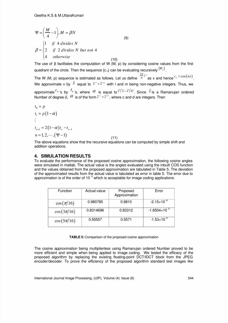
2.2 Definition: Ramanujan ordered Number of degree-2The Ramanujan ordered Number of degree-2 [11] are defined such that 2 N π is approximated bysum or difference of two numbers which are negative powers of 2. Thus Ramanujan Numbers ofdegree-2 are,
( ) ( )22
2, 1, 2,i
l m for il mι
π ι
ℜ = = (3)
( )21 , 2 2 0l ml m for m lι − −= + > ≥
( )22 , 2 2 ( 1) 0l ml m for m lι − −= − − > ≥(4)
Where l and m are integers, Hence( ) ( )21 213,5 40 1,3 10ℜ = ℜ =
Ramanujan ordered Number of degree-2 and their properties are listed in the table 2 below.
TABLE 2: Ramanujan ordered Number of Degree-2.
The accuracy of the numbers increase with the increase in the degree of the Ramanujan orderednumbers at the expense of additional shifts and additions. State-of-art technologies in Imageprocessing uses the block processing techniques for applications like image compression orimage enhancement. The standardized image block size is 8 8× , which provides us anopportunity to use Ramanujan ordered numbers to reduce the complexity of the algorithms. TableIII shows the higher degree Ramanujan ordered Numbers and their accuracies.
TABLE 3: Ramanujan ordered Number of Higher Degree.
Table 3 shows that the error of approximation decreases with the increase in the degree ofRamanujan ordered numbers, but the computational complexity also increases. Hence the choiceof Ramanujan ordered number of degree-2 is best validated for the accuracy and thecomputational overhead in computation of the cosine functions.
( ),l m ( ),l mℜ π Upper bound oferror
0,2 5 3.125 5.28x10 -3
1,2 8 3.0 4.507x10 -2
4,5 67 3.140 5.067x10 -4
( ), , .....l m p
( ), , ....l m pℜ
π Upper bound oferror
Computationalcomplexity
Shifts Adds
1,2 8 3. 0 4.507x10 -2 2 1
1,2,5 8 3.125 5.28x10 -3 3 2
1,2,5,8 8 3.1406 3.08x10 -4 4 3

8/6/2019 International Journal of Image Processing (IJIP) Volume 4 Issue 6
http://slidepdf.com/reader/full/international-journal-of-image-processing-ijip-volume-4-issue-6 33/172
Geetha K.S & M.UttaraKumari
International Journal Image Processing, (IJIP), Volume (4): Issue (6) 542
3. COSINE APPROXIMATION USING RAMANUJAN ORDERED NUMBERMethod of computing the cosine function is to find a polynomial that allows us to approximate thecosine function locally. A polynomial is a good approximation to the function near somepoint, x a= , if the derivatives of the polynomial at the point are equal to the derivatives of thecosine curve at that point. Thus the higher the degree of the polynomial, the better is the
approximation. If n p denotes the n th polynomial about x a= for a function f, and if we
approximate ( ) f x by ( ) p x at a point x, then the difference ( ) ( ) ( )n R x f x p x= −is called the n th
remainder for f about x a= . The plot of the 4 th order approximation along with the difference plotis as shown in figure 1.
FIGURE 1: Plot of f(x)=cos(x) and the remainder function .
Figure 2 indicates that the cosine approximation at various angles with 4 th degree polynomial isalmost close with the actual values. The accuracy obtained at various degrees of the polynomial
is compared in table 4. Thus we choose the 4th
degree polynomial for the cosine approximation.
FIGURE 2: Expanded version of cosine approximation.

8/6/2019 International Journal of Image Processing (IJIP) Volume 4 Issue 6
http://slidepdf.com/reader/full/international-journal-of-image-processing-ijip-volume-4-issue-6 34/172
Geetha K.S & M.UttaraKumari
International Journal Image Processing, (IJIP), Volume (4): Issue (6) 543
TABLE 4: Cosine approximation in comparison with the Actual value
The evaluation of the cosine function using the polynomial approximation is explained through theapplication of computing the Discrete Cosine Transform coefficients which uses the cosine as itsbasis function. Discrete Cosine Transforms (DCT) is widely used in the area of signal processing,
particularly for transform coding of images. Computation of DCT coefficients involves evaluationof cosine angles of multiples of 2 π /N.
The input sequence n x of size N, is transformed as, k y . The transformation may be either DFTor DCT. The DCT defined as [12]
( )1
0
2 12cos
2
0,1... 1
10
21
N k
k nn
k
n y x k
N N
for k N
for k
otherwise
ε π
ε
−
=
+ =
= −
==
∑
(5)Neglecting the scaling factors, the DCT kernel could be simplified as
( )22cos 2 2 1
0 1, 0 1
nc n k N
for n N k N
π − = +
≤ ≤ − ≤ ≤ −(6)
DCT coefficients are computed by evaluating the sequences of type
cos(2 / ), 0,1, 2...( 1), Rn nc ׀ c p n N n N pπ = = − ∈ (7)
where R is the set of real numbers. These computations are done via a Chebyshev-type ofrecursion. Let us define
( ) ( ) , cos 2w n n M p w w p n M π = =(8)
0,1, 2,.... , Rn p= Ψ ∈
Function Degree-2 Degree-4 Actual value
( )cos 16π 0.9807234 0.980785 0.980785
( )cos 3 16π 0.826510 0.831527 0.8314696
( )cos 5 16π 0.518085 0.55679 0.55557
8/6/2019 International Journal of Image Processing (IJIP) Volume 4 Issue 6
http://slidepdf.com/reader/full/international-journal-of-image-processing-ijip-volume-4-issue-6 35/172
8/6/2019 International Journal of Image Processing (IJIP) Volume 4 Issue 6
http://slidepdf.com/reader/full/international-journal-of-image-processing-ijip-volume-4-issue-6 36/172
Geetha K.S & M.UttaraKumari
International Journal Image Processing, (IJIP), Volume (4): Issue (6) 545
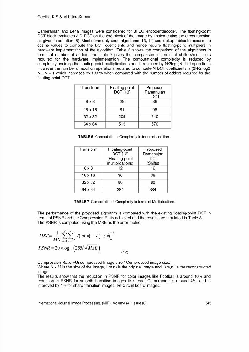
Cameraman and Lena images were considered for JPEG encoder/decoder. The floating-pointDCT block evaluates 2-D DCT on the 8x8 block of the image by implementing the direct functionas given in equation (5). Most commonly used algorithms [13, 14] use lookup tables to access thecosine values to compute the DCT coefficients and hence require floating-point multipliers inhardware implementation of the algorithm. Table 6 shows the comparison of the algorithms interms of number of adders and table 7 gives the comparison in terms of shifters/multipliersrequired for the hardware implementation. The computational complexity is reduced bycompletely avoiding the floating-point multiplications and is replaced by N/2log 2N shift operations.However the number of addition operations required to compute N DCT coefficients is (3N/2 log2N)- N + 1 which increases by 13.6% when compared with the number of adders required for thefloating-point DCT.
TABLE 6: Computational Complexity in terms of additions
TABLE 7: Computational Complexity in terms of Multiplications
The performance of the proposed algorithm is compared with the existing floating-point DCT interms of PSNR and the Compression Ratio achieved and the results are tabulated in Table 8.The PSNR is computed using the MSE as the error metric.
( ) ( )
( )
2'
1 1
10
1, ,
20 log 255
M N
m n
MSE I m n I m n MN
PSNR MSE
= =
= −
= ∗
∑∑
(12)
Compression Ratio =Uncompressed Image size / Compressed image size.Where N x M is the size of the image, I(m,n) is the original image and I`(m,n) is the reconstructedimage.The results show that the reduction in PSNR for color images like Football is around 10% andreduction in PSNR for smooth transition images like Lena, Cameraman is around 4%, and isimproved by 4% for sharp transition images like Circuit board images.
Transform Floating-pointDCT [13]
ProposedRamanujan
DCT8 x 8 29 36
16 x 16 81 96
32 x 32 209 240
64 x 64 513 576
Transform Floating-pointDCT [13]
(Floating-pointmultiplications)
ProposedRamanujan
DCT(Shifts)
8 x 8 12 12
16 x 16 36 36
32 x 32 80 80
64 x 64 384 384

8/6/2019 International Journal of Image Processing (IJIP) Volume 4 Issue 6
http://slidepdf.com/reader/full/international-journal-of-image-processing-ijip-volume-4-issue-6 37/172
Geetha K.S & M.UttaraKumari
International Journal Image Processing, (IJIP), Volume (4): Issue (6) 546
TABLE 8: Performance comparison of Ramanujan DCT and Floating-point DCT
Image Proposed Ramanujan DCT Floating-point DCT[13]Compression
RatioPSNR(dB) Compression
RatioPSNR(dB)
Circuit 5.30:1 72.93 5.6:1 69.01
Football 5.62:1 69.24 5.97:1 77.20
Lena 4.20:1 62.04 4.56:1 65.77
Medical Image 5.74:1 62.91 5.74:1 68. 1

8/6/2019 International Journal of Image Processing (IJIP) Volume 4 Issue 6
http://slidepdf.com/reader/full/international-journal-of-image-processing-ijip-volume-4-issue-6 38/172
Geetha K.S & M.UttaraKumari
International Journal Image Processing, (IJIP), Volume (4): Issue (6) 547
FIGURE3: The Original image and Reconstructed image using floating-point DCT and Ramanujan DCT.
Figure 3 shows the original image and the reconstructed image obtained using both RDCT andDCT2 function applied in JPEG compression standard technique. The difference image obtainedbetween the original and reconstructed image shows that the error in cosine approximation isvery negligible.
5. CONCLUSIONSWe have presented a method for approximation of the cosine function using Ramanujan orderednumber of degree 2. The cosine function is evaluated using a 4 th degree polynomial with an errorof approximation in the order of 10 -3 . This method allows us to evaluate the cosine function usingonly integers which are powers of 2 thereby replaces the complex floating-point multiplications byshifters & adders. This algorithm takes N/2 log 2 N shifts and (3N/2 log2 N) - N + 1 additionoperations to evaluate an N-point DCT coefficients. The cosine approximation increases theoverhead on the number of adders by 13.6%. The proposed algorithm reduces the computationalcomplexity and hence improves the speed of evaluation of the DCT coefficients. The proposedalgorithm reduces the complexity in hardware implementation using FPGA. The results show thatthe reconstructed image is almost same as obtained by evaluating the floating-point DCT.

8/6/2019 International Journal of Image Processing (IJIP) Volume 4 Issue 6
http://slidepdf.com/reader/full/international-journal-of-image-processing-ijip-volume-4-issue-6 39/172
Geetha K.S & M.UttaraKumari
International Journal Image Processing, (IJIP), Volume (4): Issue (6) 548
6. REFERENCES1. J.-M.Muller, Elementary Functions: Algorithms and Implementation, Birkhauser, Boston,
1997.
2. F.de Dinechin and A.Tisserand, “Multipartite table methods,” IEEE Transactions on
Computers, vol.54, no.3,pp. 319-330, Mar. 2005.3. M.Schulte and J. Stine, “Approximating elementary functions with symmetric bipartite tables,”
IEEE Transactions on Computers, vol. 48, no. 8, pp. 842-847, Aug. 1999.
4. J. Detrey and F.de Dinechin, “Second order function approximation using a singlemultiplication on FPGAs,” in 14th International Conference on Field-Programmable Logic andApplications, Aug.2004, pp.221-230, LNCS 3203.
5. Arnad Tisserand, “Hardware operator for simultaneous sine and cosine evaluation,” inICASSP 2006, vol III, pp.992-995.
6. N.Brisebarre, J.-M.Muller, A.Tisserand and S.Torres, “Hardware operators for functionevaluation using sparse-coefficient polynomials,” in Electronic Letters 25, 42(2006), pp. 1441-1442.
7. T Tran, “The BinDCT: Fast multiplier less approximation of the DCT”. IEEE Signal Proc. Vol.7, No. 6, pp. 141-44, 2000.
8. Y Zeng, L Cheng, G Bi, and A C Kot, “Integer DCT’s and Fast Algorithms”. IEEE Trans SignalProcessing, Vol. 49, No. 11, Nov. 2001.
9. X Hui and L Cheng, “An Integer Hierarchy: Lapped Biorthogonal Transform via Lifting Stepsand Application in Image Coding”. Proc. ICSP-02, 2002.
10. Nirdosh Bhatnagar, “On computation of certain discrete Fourier transforms using binarycalculus”.Signal Processing-Elsevier Vol43,1995.
11. Geetha.K.S, M.Uttarakumari, “Multiplierless Recursive algorithm using Ramanujan orderedNumbers,” in IETE Journal of Research, vol. 56, Issue 4, JUL-AUG 2010.
12. K.R.Rao, P.Yip, “Discrete Cosine Transform Algorithms, Advantages Applications”. NewYork: Academic 1990.
13. H.S. Hou, “A Fast Recursive Algorithms for Computing the Discrete Cosine Transform”. IEEETrans. Acoust., Speech, Signal Processing, Vol.35, pp 1455-1461, Oct 1987.
14. N.I.Cho, S.U.Lee, “A Fast 4X4 DCT Algorithm for the Recursive 2-D DCT”. IEEE Trans.Signal Processing, Vol.40, pp 2166-2173. Sep 1992.

8/6/2019 International Journal of Image Processing (IJIP) Volume 4 Issue 6
http://slidepdf.com/reader/full/international-journal-of-image-processing-ijip-volume-4-issue-6 40/172
Amiya Halder & Nilavra Pathak
International Journal of Image Processing (IJIP), Volume (4): Issue (6) 549
An Evolutionary Dynamic Clustering Based Colour ImageSegmentation
Amiya Halder [email protected] Assistant Professor
Dept. of Computer Science & Engineering St. Thomas’ College of Engg. & Technology Kolkata, West Bengal, India
Nilavra Pathak [email protected] Dept. of Computer Science & Engineering University St. Thomas’ College of Engg. & Technology Kolkata, West Bengal, India
Abstract
We have presented a novel Dynamic Colour Image Segmentation (DCIS)System for colour image. In this paper, we have proposed an efficient colourimage segmentation algorithm based on evolutionary approach i.e. dynamic GAbased clustering (GADCIS). The proposed technique automatically determinesthe optimum number of clusters for colour images. The optimal number ofclusters is obtained by using cluster validity criterion with the help of Gaussiandistribution. The advantage of this method is that no a priori knowledge isrequired to segment the color image. The proposed algorithm is evaluated onwell known natural images and its performance is compared to other clusteringtechniques. Experimental results show the performance of the proposedalgorithm producing comparable segmentation results.
Keywords: Segmentation, Clustering, Genetic Algorithm, Clustering Metric, Validity Index.
1. INTRODUCTION Image segmentation, i.e., the partitioning of an image into relevant regions, is a fundamentalproblem in image analysis. Accurate segmentation of objects of interest is often required beforefurther analysis can be performed. Despite years of active research, fully automatic segmentationof arbitrary images is still seen as an unsolved problem.
Colour image segmentation emerges as a new area of research. Colour image segmentation cansolve many contemporary problems in medical imaging, mining and mineral imaging,bioinformatics, and material sciences. Naturally, color image segmentation demands well defined
borders of different objects in an image. So, there is a fundamental demand of accuracy. Thesegmented regions or components should not be further away from the true object than one or afew pixels. So, there is a need for an improved image segmentation technique that can segmentdifferent components precisely. Image data have some particular characteristics that differentiatethem from other form of data. Image data may have corrupted values due to the usual limitationsor artifacts of imaging devices. Noisy data, data sparsity, and high dimensionality of data createdifficulties in image pixel clustering. As a result, image pixel clustering becomes a harder problemthan other form of data. Although there are some existing algorithms for unsupervised colorimage segmentation, none of them has been found to be robust in determining an accuratenumber of components or segments. Image segmentation is a very important field in image

8/6/2019 International Journal of Image Processing (IJIP) Volume 4 Issue 6
http://slidepdf.com/reader/full/international-journal-of-image-processing-ijip-volume-4-issue-6 41/172
Amiya Halder & Nilavra Pathak
International Journal of Image Processing (IJIP), Volume (4): Issue (6) 550
analysis, object recognition, image coding and medical imaging. Segmentation is very challengingbecause of the multiplicity of objects in an image and the large variation between them. Imagesegmentation is the process of division of the image into regions with similar attributes.
The method for the segmentation of digital images can be broadly classified in: (a) edge and lineoriented segmentation, (b) region growing methods, (c) clustering, and (d) region splittingmethods. Edge and line oriented segmentation work on either individually analyzing each databand or considering the whole vector space. After edge extraction, a processing should beapplied to create objects and segments that represent the elements present in the scene. Regiongrowing and splitting method deals commonly with feature extraction and thresholding. In manyobject based image segmentation applications, the number of cluster is known a priori, but ourproposed scheme is automatically determined the optimal number of clustering. The proposedtechnique should be able to provide good optimal results whereas the K-means algorithm whichmay get stuck at values which are not optimal [16]. Some of the several unsupervised clusteringalgorithms developed include K-means [13, 14], fuzzy K-means, ISODATA [11], self-organizingfeature map (SOM) [15], particle swarm optimization (PSO) [10], learning vector quantizers (LVQ)[12], Dynamic GA based Clustering [17] etc.
Colour images are more complex than gray scale images as instead of a single intensity value fora pixel, each pixel is usually denoted by three component values such as Red, Green and Blue.Clustering based methods are ideal to use for gray scale images can be easily extended to copewith higher dimensity, although, the increased dimensionality also leads to more computationallyexpensive process. Various segmentation techniques have been developed for imagesegmentation include Unsupervised Colour Textured Image Segmentation Using ClusterEnsembles and MRF Model [18], Determination of Number of Clusters in k-means Clustering andapplication in Colour Image Segmentation [20], Unsupervised Colour Image Segmentation basedon Gaussian Mixture Model [21] etc.
This paper presents automatic image segmentation of colour images using GA-based clustering.One natural view of segmentation is that we are attempting to determine which components of adata set naturally “belong together”. Clustering is a process whereby a data set is replaced byclusters, which are collections of data points that “belong together”. Thus, it is natural to think ofimage segmentation as image clustering i.e. the representation of an image in terms of clusters of
pixels that “belong together”. The specific criterion to be used depends on the application. Pixelsmay belong together because of the same colour or similarity measure.
Natural colour images are particularly noisy due to the environment they were produced.Therefore, it is hard to develop a robust and faithful unsupervised technique for automaticdetermination of number of objects in a colour image. Although there are a few existingapproaches for unsupervised colour image segmentation, none of them has been found robust inall situation. Initially we tried SNOB [8], a Minimum Message Length (MML) based unsuperviseddata clustering approach to address this problem [19].
Genetic Algorithm based clustering technique has been used to cluster datasets [1-5]. In thispaper we present an efficient image segmentation algorithm using automatic GA based clusteringalgorithm. The result of this algorithm produced a better result to compare with other techniques.
The rest of the paper is organized in the following manner: Section II introduces GeneticAlgorithms. Section III gives an overview of the GA based clustering approach. Proposedalgorithm is discussed in section IV. Section V summarizes the experimental results.
2. GENETIC ALGORITHM Genetic Algorithm (GA) is a population-based stochastic search procedure to find exact orapproximate solutions to optimization and search problems. Modeled on the mechanisms ofevolution and natural genetics, genetic algorithms provide an alternative to traditional optimization

8/6/2019 International Journal of Image Processing (IJIP) Volume 4 Issue 6
http://slidepdf.com/reader/full/international-journal-of-image-processing-ijip-volume-4-issue-6 42/172

8/6/2019 International Journal of Image Processing (IJIP) Volume 4 Issue 6
http://slidepdf.com/reader/full/international-journal-of-image-processing-ijip-volume-4-issue-6 43/172
Amiya Halder & Nilavra Pathak
International Journal of Image Processing (IJIP), Volume (4): Issue (6) 552
Subsequently, the clustering metric M is computed as the sum of Euclidean distances of eachpoint from their respective cluster centers given by
,
1
i
K
i
M M ∑=
=
(3)
∑∈
−=
i jC x
i ji bgr zbgr x M ||),,(),,(|| (4)
The fitness function is defined asf = 1/M. (5)
A low value of intra-cluster spread is a characteristic of efficient clustering. Hence our objective isto minimize the clustering metric M i.e. maximize f.
3.4 SelectionThis paper employs the Roulette Wheel selection - a proportional selection mechanism in whichthe number of copies of a chromosome, that go into the mating pool for subsequent operations, isproportional to its fitness.
3.5 CrossoverIn this paper we use single-point crossover with a fixed crossover probability of µ c. The procedure
followed is the same as that described in section 2.3.6 MutationEach chromosome undergoes mutation with a fixed probability µ m. A number δ in the range [0, 1]is generated with uniform distribution. If the value at a gene position is v, after mutation itbecomes
v ± δ * v, v ≠ 0v ± δ , v = 0. (6)
3.7 Termination criterionWe execute the processes of fitness computation, selection, crossover, and mutation for apredetermined number of iterations. In every generational cycle, the fittest chromosome till thelast generation is preserved - elitism. Thus on termination, this chromosome gives us the bestsolution encountered during the search.
4. PROPOSED METHODWe proposed a new segmentation algorithm that can produce a new result according to thevalues of the clustering. We consider a colour image f of size mxn. The proposed algorithm is:
1. Repeat steps 2 to 8 for K=2 to K=K max.2. Initialize the P chromosomes of the population.3. Compute the fitness function f i for i=1,…,P, using equation (5).4. Preserve the best (fittest) chromosome seen till that generation.5. Apply Roulette Wheel selection on the population.6. Apply crossover and mutation on the selected population according
to sections 3.5 and 3.6 respectively.7. Repeat steps 3 to 6 till termination condition is reached.8. Compute the clustering Validity Index for the fittest chromosome for
the particular value of K, using equation (7), in order to determine thevalidity of the clustering on the given dataset.
9. Cluster the dataset using the most appropriate number of clustersdetermined by comparing the Validity Indices of the proposedclusters for K=2 to K=K max .

8/6/2019 International Journal of Image Processing (IJIP) Volume 4 Issue 6
http://slidepdf.com/reader/full/international-journal-of-image-processing-ijip-volume-4-issue-6 44/172
Amiya Halder & Nilavra Pathak
International Journal of Image Processing (IJIP), Volume (4): Issue (6) 553
4.1 Validity IndexThe cluster validity measure used in the paper is the one proposed by Turi [8]. It aims atminimizing the validity index given by the function,
inter intra
yV ×=
(7)The term intra is the average of all the distances between each pixel x(r,g,b) and its clustercentroid z i(r,g,b) which is defined as
2
1
||),,(),,(||N1 ∑∑
∈=
−=
iC xi
K
i
bgr zbgr xintra (8)
Where ||x(r,g,b) – z i(r,g,b)|| means the Euclidean distance, which is calculated as√(xred – z ired )2 + (x green – z igreen )2 + (xblue – z iblue )2,
where N is the total number of pixels, C i is the cluster number, z i is the centroids of cluster C i, K isthe total number of clusters. Intra cluster dependency is the sum of square of Euclidean distanceof every element from the centroids of the cluster to which it belongs.On the other hand, inter is the inter cluster dependency which gives the idea about the extent towhich each clusters are related. The higher this value the better clustering is obtained. It isrepresented as
K i jK i
wherebgr j zbgr i zinter
,...,1,1,...2,1
),2||),,(),,(min(||
+=−=
−= (9)
and Z i and Z j are the centroids. Intra cluster dependency is the minimum of the square ofEuclidean distances of each centroids from the other.Lastly, y is given as
1)1,2( +×= N c y (10)Where c is a constant (selected value is 25), N(2,1) is a Gaussian distribution function with mean
2 and standard deviation 1, where the variable is the cluster number and is given as
2
2
2
)(
22
1),( σ
µ
πσ σ µ
−
=
k
e N (11)
Where K is the cluster number and µ=2 and σ=1 as per Turi’s thesis on clustering. This is done tonegate the occurrence of lower number of clusters 2 or 3.This validity measure serves the dual purpose of
• minimizing the intra-cluster spread, and• maximizing the inter-cluster distance.
Moreover it overcomes the tendency to select a smaller number of clusters (2 or 3) as optimal,which is an inherent limitation of other validity measures such as the Davies-Bouldin index orDunne’s index.
5. EXPERIMENTAL RESULTSThe proposed algorithm has been applied to well known natural colour images such as Lena,mandrill and peppers etc. All the results have been reported in Table 1. Column 2 of Table 1represent the optimal range for the number of clusters for the images of Lena, mandrill andpeppers etc have also been copied from [8] which is based on visual analysis by a group of tenexpert people. These results have been compared to those of SOM and DCPSO [9] and to that ofsnob [8]. The results tabulated here for each image is the mean of 10 simulations. Figure1 areshown the some segmented output images using our proposed clustering method. The result ofTABLE 1 is shows better than SOM and snob and always find a solution within the optimal range.The performance of the proposed algorithm with DCPSO produced comparable segmentationresults [9].

8/6/2019 International Journal of Image Processing (IJIP) Volume 4 Issue 6
http://slidepdf.com/reader/full/international-journal-of-image-processing-ijip-volume-4-issue-6 45/172
Amiya Halder & Nilavra Pathak
International Journal of Image Processing (IJIP), Volume (4): Issue (6) 554
The assumptions used for the implementation of the proposed algorithm are given as follows. Thevalue of the parameter, c, for the validity index referred to from [8], is set to 25. The size of thepopulation, P, is taken as 30, crossover rate, µ c, as 0.9 and mutation rate, µ m, as 0.01 [6]. Thealgorithm uses number of iterations as the terminating condition and it is set to 20. The value ofKmax is empirically set for the individual images.
Table 1: Experiment of some natural images
Image OptimalRange
ProposedMethod
DCPSOusing
VSOM Snob
Lena 5 to 10 5 6.85 20 31Peppers 6 to 10 6.7 6.25 20 42Mandrill 5 to 10 6.5 6 20 39
Jet 5 to 7 6 5.3 14 22Duck - 7.2 - - -
Baboon - 5.9 - - -F16 - 6.6 - - -
Parrot - 7.1 - - -
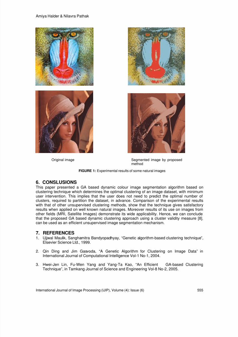
8/6/2019 International Journal of Image Processing (IJIP) Volume 4 Issue 6
http://slidepdf.com/reader/full/international-journal-of-image-processing-ijip-volume-4-issue-6 46/172
Amiya Halder & Nilavra Pathak
International Journal of Image Processing (IJIP), Volume (4): Issue (6) 555
6. CONSLUSIONSThis paper presented a GA based dynamic colour image segmentation algorithm based onclustering technique which determines the optimal clustering of an image dataset, with minimumuser intervention. This implies that the user does not need to predict the optimal number ofclusters, required to partition the dataset, in advance. Comparison of the experimental resultswith that of other unsupervised clustering methods, show that the technique gives satisfactoryresults when applied on well known natural images. Moreover results of its use on images fromother fields (MRI, Satellite Images) demonstrate its wide applicability. Hence, we can concludethat the proposed GA based dynamic clustering approach using a cluster validity measure [8],can be used as an efficient unsupervised image segmentation mechanism.
7. REFERENCES1. Ujjwal Maulik, Sanghamitra Bandyopadhyay, “Genetic algorithm-based clustering technique”,
Elsevier Science Ltd., 1999.
2. Qin Ding and Jim Gasvoda, “A Genetic Algorithm for Clustering on Image Data” inInternational Journal of Computational Intelligence Vol-1 No-1, 2004.
3. Hwei-Jen Lin, Fu-Wen Yang and Yang-Ta Kao, “An Efficient GA-based ClusteringTechnique”, in Tamkang Journal of Science and Engineering Vol-8 No-2, 2005.
FIGURE 1: Experimental results of some natural images
Original image Segmented image by proposedmethod
8/6/2019 International Journal of Image Processing (IJIP) Volume 4 Issue 6
http://slidepdf.com/reader/full/international-journal-of-image-processing-ijip-volume-4-issue-6 47/172
Amiya Halder & Nilavra Pathak
International Journal of Image Processing (IJIP), Volume (4): Issue (6) 556
4. Rafael C. Gonzalez, Richard E. Woods, Digital Image Processing, Pearson Education, 2002.
5. R. C. Dubes, A. K. Jain, “Clustering techniques: the user’s dilemma”, Pattern Recognition,1976.
6. M. Srinivas, Lalit M. Patnaik, “Genetic Algorithms: A Survey”.
7. D. E. Goldberg, Genetic Algorithms in Search, Optimization and Machine Learning, Addison-Wesley, 1989.
8. R. H. Turi, “Clustering-Based Color Image Segmentation”, PhD Thesis, Monash University,Australia, 2001.
9. Mahamed G. H. Omran, Andries P Engelbrecht and Ayed Salman, “Dynamic Clustering usingParticle Swarm Optimization with Application in Unsupervised Image Classification”,PWASET Volume 9, 2005.
10. DW van der Merwe, AP Engelbrecht, “Data Clustering using Particle Swarm Optimization”.
11. G Ball, D Hall, “A Clustering Technique for Summarizing Multivariate Data”, BehavioralScience, Vol. 12, 1967.
12. LV Fausett, “Fundamentals of Neural Networks”, Prentice Hall, 1994.
13. E Forgy, “Cluster Analysis of Multivariate Data: Efficiency versus Interpretability ofClassification”, Biometrics, Vol. 21, 1965.
14. JA Hartigan, Clustering Algorithms, John Wiley & Sons, New York, 1975.
15. T Kohonen, “Self-Organizing Maps”, Springer Series in Information Sciences, Vol 30,Springer-Verlag, 1995.
16. S.Z. Selim, M.A. Ismail, K-means type algorithms: a generalized convergence theorem and
characterization of local optimality, IEEE Trans. Pattern Anal. Mach. Intell.6 (1984) 81-87.
17. Dipak Kumar Kole and Amiya Halder ,“ An Efficient Image Segmentation Algorithm usingDynamic GA based Clustering”, International Journal of Logistics and Supply ChainManagement , Vol. 2, No. 1,pp.17-20, 2010.
18. Mofakharul Islam, John Yearwood and Peter Vamplew “Unsupervised Color Textured ImageSegmentation Using Cluster Ensembles and MRF Model”, Advances in Computer andInformation Sciences and Engineering, 323–328. © Springer Science+Business Media B.V.2008.
19. C.S. Wallace, and D..L. Dow, “MML clustering of multi-state, poisson, von mises circular andgaussian distribution”, Statistics and Computing,Vol.10(1), Jan. 2000, pp.73-83.
20. R. Siddheswar and R.H. Turi, “Determination of Number of Clusters in k-means Clusteringand application in Color Image Segmentation”, In Proceedings of the 4th Intl. Conf. onAdvances in Pattern Recognition and Digital Techniques (ICAPRDT’99), vol. Calcutta, India,1999 pages: 137-143.
21. Wu Yiming, Yang Xiangyu, and Chan Kap Luk, “Unsupervised Color Image Segmentationbased on Gaussian Mixture Model”, In Proceedings of the 2003 Joint Conf. of the 4th Intl.Conf. on Information, Communications and Signal Processing, Vol. 1(15-18 Dec. 2003),pages: 541-544.
8/6/2019 International Journal of Image Processing (IJIP) Volume 4 Issue 6
http://slidepdf.com/reader/full/international-journal-of-image-processing-ijip-volume-4-issue-6 48/172
Phei-Chin Lim, Narayanan Kulathuramaiyer & Dayang NurFatimah Awg. Iskandar
International Journal of Image Processing (IJIP), Volume (4): Issue (6) 557
Towards Semantic Clustering – A Brief Overview
Phei-Chin Lim [email protected] of Computer Science and Information Technology
Universiti Malaysia Sarawak 94300 Kota Samarahan, Sarawak, Malaysia
Narayanan Kulathuramaiyer [email protected] of Computer Science and Information Technology Universiti Malaysia Sarawak 94300 Kota Samarahan, Sarawak, Malaysia
Dayang NurFatimah Awg. Iskandar [email protected] of Computer Science and Information Technology Universiti Malaysia Sarawak 94300 Kota Samarahan, Sarawak, Malaysia
Abstract
Image clustering is an important technology which helps users to get hold of thelarge amount of online visual information, especially after the rapid growth of theWeb. This paper focuses on image clustering methods and their application inimage collection or online image repository. Current progress of image clusteringrelated to image retrieval and image annotation are summarized and some openproblems are discussed. Related works are summarized based on the problemsaddressed, which are image segmentation, compact representation of image set,search space reduction, and semantic gap. Issues are also identified in currentprogress and semantic clustering is conjectured to be the potential trend. Ourframework of semantic clustering as well as the main abstraction levels involvedis briefly discussed.
Keywords: Image Clustering, Semantic Gap, Semantic Clustering, Concept Description, SymbolicDescription.
1. INTRODUCTION
Advancement in digital imaging devices, technology and cost-decrease in storage devicescontributed to the creation of large-scale digital images in various domains. The question now ishow to effectively extract semantically meaningful information (knowledge) from these imagecollections. One of the fundamental of understanding and learning is to discover the naturalgroupings of images based on similarity of multiple characteristics or latent aspects of meaning.In this paper, the former referred to image clustering while the latter leads to semantic clustering.
One of the reasons for writing this paper is that we hardly find any work in reviewing imageclustering methods by highlighting the challenges and provide association between imageclustering and semantic clustering. Semantic clustering has attracted many research efforts afterthe year 2000 in terms of papers published. A simple experiment is conducted where wesearched for publications containing the phrases image clustering and semantic clustering using
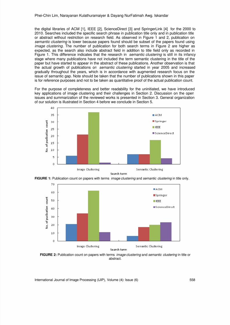
8/6/2019 International Journal of Image Processing (IJIP) Volume 4 Issue 6
http://slidepdf.com/reader/full/international-journal-of-image-processing-ijip-volume-4-issue-6 49/172
Phei-Chin Lim, Narayanan Kulathuramaiyer & Dayang NurFatimah Awg. Iskandar
International Journal of Image Processing (IJIP), Volume (4): Issue (6) 558
the digital libraries of ACM [1], IEEE [2], ScienceDirect [3] and SpringerLink [4] for the 2000 to2010. Searches included the specific search phrase in publication title only and in publication titleor abstract without restriction on research field. As observed in Figure 1 and 2, publication onsemantic clustering is lower because papers found should be subset of the papers found using image clustering. The number of publication for both search terms in Figure 2 are higher asexpected, as the search also include abstract field in addition to title field only as recorded inFigure 1. This difference indicates that the research in semantic clustering is still in its infancystage where many publications have not included the term semantic clustering in the title of thepaper but have started to appear in the abstract of these publications. Another observation is thatthe actual growth of publications on semantic clustering started in year 2005 and increasedgradually throughout the years, which is in accordance with augmented research focus on theissue of semantic gap. Note should be taken that the number of publications shown in this paperis for reference purposes and not to be taken as quantitative proof of the actual publication count.
For the purpose of completeness and better readability for the uninitiated, we have introducedkey applications of image clustering and their challenges in Section 2. Discussion on the openissues and summarization of the reviewed works is presented in Section 3. General organizationof our solution is illustrated in Section 4 before we conclude in Section 5.
FIGURE 1: Publication count on papers with terms image clustering and semantic clustering in title only.
FIGURE 2: Publication count on papers with terms image clustering and semantic clustering in title orabstract.
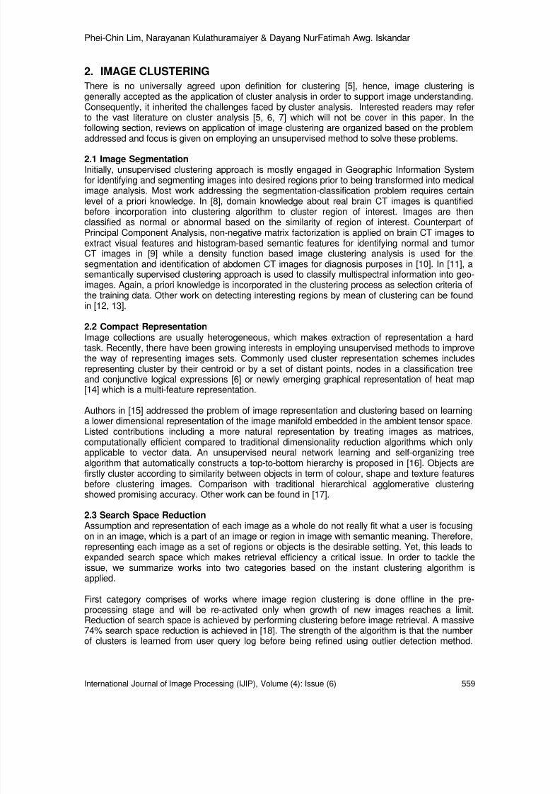
8/6/2019 International Journal of Image Processing (IJIP) Volume 4 Issue 6
http://slidepdf.com/reader/full/international-journal-of-image-processing-ijip-volume-4-issue-6 50/172
Phei-Chin Lim, Narayanan Kulathuramaiyer & Dayang NurFatimah Awg. Iskandar
International Journal of Image Processing (IJIP), Volume (4): Issue (6) 559
2. IMAGE CLUSTERINGThere is no universally agreed upon definition for clustering [5], hence, image clustering isgenerally accepted as the application of cluster analysis in order to support image understanding.Consequently, it inherited the challenges faced by cluster analysis. Interested readers may referto the vast literature on cluster analysis [5, 6, 7] which will not be cover in this paper. In thefollowing section, reviews on application of image clustering are organized based on the problem
addressed and focus is given on employing an unsupervised method to solve these problems.
2.1 Image SegmentationInitially, unsupervised clustering approach is mostly engaged in Geographic Information Systemfor identifying and segmenting images into desired regions prior to being transformed into medicalimage analysis. Most work addressing the segmentation-classification problem requires certainlevel of a priori knowledge. In [8], domain knowledge about real brain CT images is quantifiedbefore incorporation into clustering algorithm to cluster region of interest. Images are thenclassified as normal or abnormal based on the similarity of region of interest. Counterpart ofPrincipal Component Analysis, non-negative matrix factorization is applied on brain CT images toextract visual features and histogram-based semantic features for identifying normal and tumorCT images in [9] while a density function based image clustering analysis is used for thesegmentation and identification of abdomen CT images for diagnosis purposes in [10]. In [11], a
semantically supervised clustering approach is used to classify multispectral information into geo-images. Again, a priori knowledge is incorporated in the clustering process as selection criteria ofthe training data. Other work on detecting interesting regions by mean of clustering can be foundin [12, 13].
2.2 Compact RepresentationImage collections are usually heterogeneous, which makes extraction of representation a hardtask. Recently, there have been growing interests in employing unsupervised methods to improvethe way of representing images sets. Commonly used cluster representation schemes includesrepresenting cluster by their centroid or by a set of distant points, nodes in a classification treeand conjunctive logical expressions [6] or newly emerging graphical representation of heat map[14] which is a multi-feature representation.
Authors in [15] addressed the problem of image representation and clustering based on learninga lower dimensional representation of the image manifold embedded in the ambient tensor space.Listed contributions including a more natural representation by treating images as matrices,computationally efficient compared to traditional dimensionality reduction algorithms which onlyapplicable to vector data. An unsupervised neural network learning and self-organizing treealgorithm that automatically constructs a top-to-bottom hierarchy is proposed in [16]. Objects arefirstly cluster according to similarity between objects in term of colour, shape and texture featuresbefore clustering images. Comparison with traditional hierarchical agglomerative clusteringshowed promising accuracy. Other work can be found in [17].
2.3 Search Space ReductionAssumption and representation of each image as a whole do not really fit what a user is focusingon in an image, which is a part of an image or region in image with semantic meaning. Therefore,representing each image as a set of regions or objects is the desirable setting. Yet, this leads toexpanded search space which makes retrieval efficiency a critical issue. In order to tackle theissue, we summarize works into two categories based on the instant clustering algorithm isapplied.
First category comprises of works where image region clustering is done offline in the pre-processing stage and will be re-activated only when growth of new images reaches a limit.Reduction of search space is achieved by performing clustering before image retrieval. A massive74% search space reduction is achieved in [18]. The strength of the algorithm is that the numberof clusters is learned from user query log before being refined using outlier detection method.

8/6/2019 International Journal of Image Processing (IJIP) Volume 4 Issue 6
http://slidepdf.com/reader/full/international-journal-of-image-processing-ijip-volume-4-issue-6 51/172
Phei-Chin Lim, Narayanan Kulathuramaiyer & Dayang NurFatimah Awg. Iskandar
International Journal of Image Processing (IJIP), Volume (4): Issue (6) 560
Authors in [19] proposed an interactive approach where user’s feedback on initial search resultsis required for analyzing user interest. Both works make use of Corel image sets.
Clustering is performed online in the post-processing stage in the second category. In [20],search results from initial query are clustered into semantic groups together with learned labelswhich provide overview of the content of the results. Users are able to browse through eachcluster easily. Similar work can be found in [21, 22]. Humans have higher tendency to use high-level abstract concepts (image semantics) during querying or browsing of image collection ratherthan using low-level visual features. Consequently, huge amount of irrelevant search results arereturned due to the semantic gap described in the previous section. For this reason, clustersearch results are converted into symbolically similar clusters in order to filter out therelevant/irrelevant images in [23].
2.4 Semantic GapContent-based Image Retrieval (CBIR) is the technology that organizes digital images by theirvisual content which was haunted by the critical challenge of the semantic gap being defined as“the lack of coincidence between the information that one can extract from the visual data and theinterpretation that the same data have for a user in a given situation” [24]. Several taxonomies ofmethods in addressing the problem of semantic gap were suggested in [25] and [26]. Clusteringis adapted in CBIR to solve the semantic gap issue starting mid 2000’s onwards.
In a typical CBIR system, query results are a set of images sorted by feature similarities but thereis no guarantee that the returned images will be similar in semantic as shown in Figure 3 (a).Figure 3 (b) showed the result of retrieved images that are similar in semantic and content [27],where butterfly wing images were firstly clustered into semantic shape categories beforeperforming similarity search to ensure only images in the same shape category are considered infinding similar images to the query. CLUE [28] approach the same issue differently by groupingsemantically similar images with respect to query and return image clusters instead of a set ofordered images. Similar work was done in [20, 21, 29].
(a)
(b)FIGURE 3: Ten most similar images retrieved (query image in highlighted), (a) conventional similarity-based
approach, (b) semantic shape category from [27].
3. OPEN ISSUESIn brief, image clustering is the organization of images into different clusters (groups, classes orcategories) based on similarity such that images in the same cluster share some commoncharacteristics. A crucial issue of image clustering on large-scale image repository is compactrepresentation for faster image indexing and searching. The derived clusters providesummarization of the image content that can be utilized for tasks such as image search andbrowsing. Refer to Table 1 for summarization of selected works that employed clusteringalgorithms.

8/6/2019 International Journal of Image Processing (IJIP) Volume 4 Issue 6
http://slidepdf.com/reader/full/international-journal-of-image-processing-ijip-volume-4-issue-6 52/172
Phei-Chin Lim, Narayanan Kulathuramaiyer & Dayang NurFatimah Awg. Iskandar
International Journal of Image Processing (IJIP), Volume (4): Issue (6) 561
Problem Authors Feature Approach ClusterDescription
Image Segmentation Pan et.al [8] Object’s graylevel, size,location,elongation,direction
Object clusteringfollowed by imageclustering
Normal/Abnormal
Liu et.al [9] Visual features;histogram-basedsemantic features
Non-negativeMatrixFactorization
Normal/Tumor
Torres et.al [11] Spatial semantics(geometrical &topologicalproperties)
MaximumLikelihood
Categories label(water, urban,crop, landslide,vegetation etc)
Han et.al [13] Texturehomogeneity
Self-organizingfeature map,agglomerativeclustering
Nil
SearchSpaceReduction
Beforeretrieval
Liu et.al [18] 3 texture features,2 shape features,27 colour features
Affinity matrixclustering,network flow -based outlierdetection (refineclustering result)
Nil
Zhang & Chen[19]
13 colour features,6 texture features
Genetic algorithm Categories label(horse, eagle,flower, fish, glassetc)
Afterretrieval
Wang et.al [22] 6 color moments,44 auto-correlogram, 14colour-texturemoments;keywords (fromimage titles &description)
K-means; ImageFrequency-Inverse KeywordFrequency; Random Walkwith Restarts
Annotations
Tahayna et.al[23] 11 colour words,11 texture words,8 shape words
Three-layer fuzzypartitioning Nil
CompactRepresentation
He et.al [15] 32x32dimensionalmatrix
K-means Nil
Wang & Khan[16]
Object’s shape,colour & texturefeatures
Dynamic GrowingSelf-OrganizingTree
Nil
Semantic Gap Lim et.al [27] Shape features k-Means Visual concept &itscharacterization
Chen et.al [28] 3 average colours,3 texture features
K-means; Graph-theoreticclustering
Nil
Wang et.al [20] Textual features(phrases)
Salient phraseranking, ImageSearch ResultClustering
10-50 final clusternames(dependent onquery word) aftermerge & prune,other cluster
Gao et.al [29] Colour histogram,texture histogram
Kernel-basedclustering
Nil
TABLE 1: Summarization of selected works on image clustering.
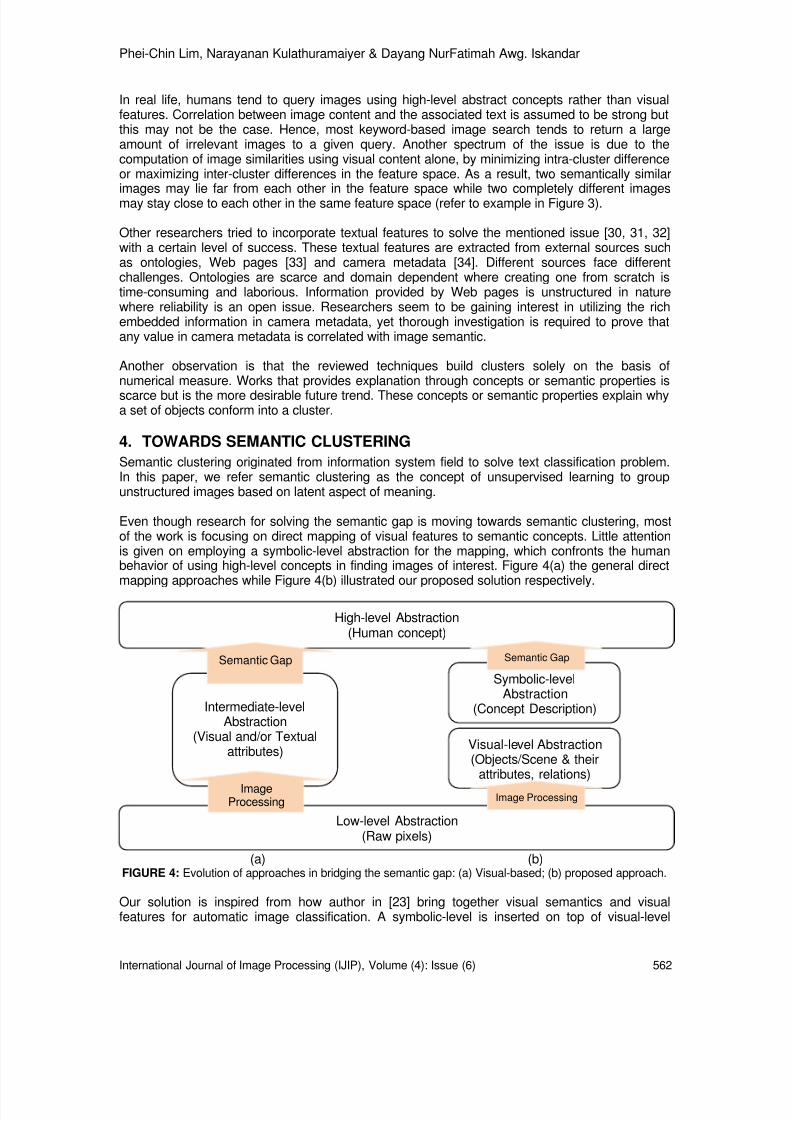
8/6/2019 International Journal of Image Processing (IJIP) Volume 4 Issue 6
http://slidepdf.com/reader/full/international-journal-of-image-processing-ijip-volume-4-issue-6 53/172
Phei-Chin Lim, Narayanan Kulathuramaiyer & Dayang NurFatimah Awg. Iskandar
International Journal of Image Processing (IJIP), Volume (4): Issue (6) 562
In real life, humans tend to query images using high-level abstract concepts rather than visualfeatures. Correlation between image content and the associated text is assumed to be strong butthis may not be the case. Hence, most keyword-based image search tends to return a largeamount of irrelevant images to a given query. Another spectrum of the issue is due to thecomputation of image similarities using visual content alone, by minimizing intra-cluster differenceor maximizing inter-cluster differences in the feature space. As a result, two semantically similarimages may lie far from each other in the feature space while two completely different imagesmay stay close to each other in the same feature space (refer to example in Figure 3).
Other researchers tried to incorporate textual features to solve the mentioned issue [30, 31, 32]with a certain level of success. These textual features are extracted from external sources suchas ontologies, Web pages [33] and camera metadata [34]. Different sources face differentchallenges. Ontologies are scarce and domain dependent where creating one from scratch istime-consuming and laborious. Information provided by Web pages is unstructured in naturewhere reliability is an open issue. Researchers seem to be gaining interest in utilizing the richembedded information in camera metadata, yet thorough investigation is required to prove thatany value in camera metadata is correlated with image semantic.
Another observation is that the reviewed techniques build clusters solely on the basis ofnumerical measure. Works that provides explanation through concepts or semantic properties isscarce but is the more desirable future trend. These concepts or semantic properties explain whya set of objects conform into a cluster.
4. TOWARDS SEMANTIC CLUSTERINGSemantic clustering originated from information system field to solve text classification problem.In this paper, we refer semantic clustering as the concept of unsupervised learning to groupunstructured images based on latent aspect of meaning.
Even though research for solving the semantic gap is moving towards semantic clustering, mostof the work is focusing on direct mapping of visual features to semantic concepts. Little attentionis given on employing a symbolic-level abstraction for the mapping, which confronts the humanbehavior of using high-level concepts in finding images of interest. Figure 4(a) the general directmapping approaches while Figure 4(b) illustrated our proposed solution respectively.
(a) (b)FIGURE 4: Evolution of approaches in bridging the semantic gap: (a) Visual-based; (b) proposed approach.
Our solution is inspired from how author in [23] bring together visual semantics and visualfeatures for automatic image classification. A symbolic-level is inserted on top of visual-level
Low-level Abstraction(Raw pixels)
Intermediate-levelAbstraction
(Visual and/or Textualattributes)
High-level Abstraction(Human concept)
Semantic Gap
Symbolic-levelAbstraction
(Concept Description)
Semantic Gap
ImageProcessing
Visual-level Abstraction(Objects/Scene & their
attributes, relations)
Image Processing
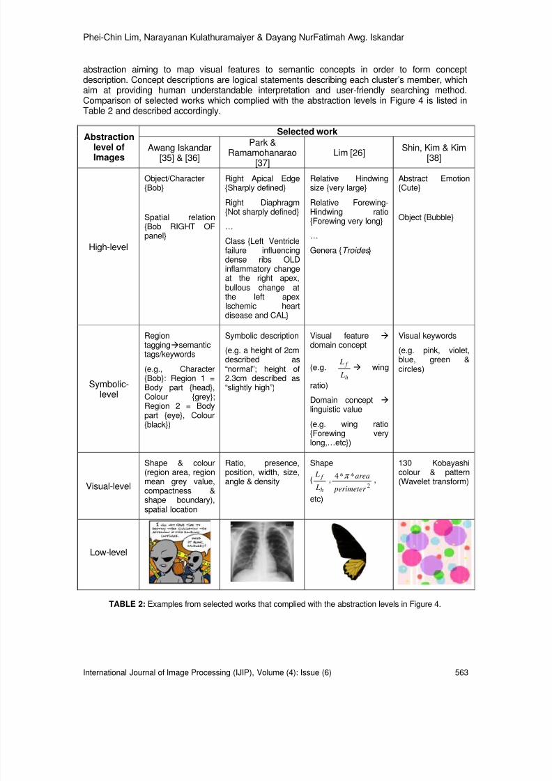
8/6/2019 International Journal of Image Processing (IJIP) Volume 4 Issue 6
http://slidepdf.com/reader/full/international-journal-of-image-processing-ijip-volume-4-issue-6 54/172
Phei-Chin Lim, Narayanan Kulathuramaiyer & Dayang NurFatimah Awg. Iskandar
International Journal of Image Processing (IJIP), Volume (4): Issue (6) 563
abstraction aiming to map visual features to semantic concepts in order to form conceptdescription. Concept descriptions are logical statements describing each cluster’s member, whichaim at providing human understandable interpretation and user-friendly searching method.Comparison of selected works which complied with the abstraction levels in Figure 4 is listed inTable 2 and described accordingly.
Abstractionlevel ofImages
Selected work
Awang Iskandar[35] & [36]
Park &Ramamohanarao
[37]Lim [26] Shin, Kim & Kim
[38]
High-level
Object/CharacterBob
Spatial relationBob RIGHT OFpanel
Right Apical EdgeSharply defined
Right DiaphragmNot sharply defined
…
Class Left Ventriclefailure influencingdense ribs OLDinflammatory changeat the right apex,bullous change atthe left apexIschemic heartdisease and CAL
Relative Hindwingsize very large
Relative Forewing-Hindwing ratioForewing very long
…
Genera Troides
Abstract EmotionCute
Object Bubble
Symbolic-level
Regiontagging semantictags/keywords
(e.g., CharacterBob: Region 1 =Body part head,Colour grey;Region 2 = Bodypart eye, Colourblack)
Symbolic description
(e.g. a height of 2cmdescribed as“normal”; height of2.3cm described as“slightly high”)
Visual feature domain concept
(e.g.h
f
L
Lwing
ratio)
Domain concept
linguistic value(e.g. wing ratioForewing verylong,…etc)
Visual keywords
(e.g. pink, violet,blue, green &circles)
Visual-level
Shape & colour(region area, regionmean grey value,compactness &shape boundary),spatial location
Ratio, presence,position, width, size,angle & density
Shape
(h
f
L
L,
2
**4
perimeter
areaπ ,
etc)
130 Kobayashicolour & pattern(Wavelet transform)
Low-level
TABLE 2: Examples from selected works that complied with the abstraction levels in Figure 4.

8/6/2019 International Journal of Image Processing (IJIP) Volume 4 Issue 6
http://slidepdf.com/reader/full/international-journal-of-image-processing-ijip-volume-4-issue-6 55/172
Phei-Chin Lim, Narayanan Kulathuramaiyer & Dayang NurFatimah Awg. Iskandar
International Journal of Image Processing (IJIP), Volume (4): Issue (6) 564
Although these selected works are successfully mapped with all the abstraction levels, richnessof high-level concept is different. For example, the high-level concept [35] is object label (“comiccharacter”) where the usage is to query relevant comic strips, while [38] tried to map colour andpattern to emotional concepts (“Cute”, “Classic”) in textile domain. Emotional concepts areabstract attributes to describe images and the most difficult indexing level because it is highlysubjective and assessments among different users vary greatly. For example, sample textileimage in Table 2 may represent “Cute” to one person but “Romantic” to another. Both works donot provide concept description as compared to [26] and [37].
In [37], image features are firstly extracted and analyzed before converted to symbolicdescriptions by fuzzy functions (refer to example given in Table 2). Hence, an expert (radiologist)can work with linguistic terms instead of numerical description of object features. Same in [26],visual features are extracted from salient regions before being converted to domain concepts andthen further characterization. As final result, each butterfly genera is represented by theircorresponding descriptions which is human understandable.
5. CONCLUDING REMARKSThis paper provided an overview of works on image clustering and discussed the challengesfaced which led to the shift to semantic clustering. Recent works mostly formed clusters using
low-level visual features and directly mapped clusters to high-level human concepts, which islimited in semantic richness. Even though there are attempts to incorporate textual information toenrich image understanding, there is still lack in providing cluster (concept) description.Therefore, a system that is capable to describe clusters symbolically which highlight theinterpretability of clusters is highly desired.
6. REFERENCES1. ACM – Association for Computing Machinery, http://www.acm.org . Accessed November
2010.
2. IEEE – Institute of Electronic and Electrical Engineers, http://ieeexplore.ieee.org . AccessedNovember 2010.
3. ScienceDirect, http://www.sciencedirect.com . Accessed November 2010.
4. SpringerLink, http://www.springerlink.com . Accessed November 2010.
5. B.S. Everitt. “ Cluster Analysis” (3 rd Edition), Edward Arnold, Ltd., London, UK, 1993.
6. A.K. Jain, M.N. Murty and P.J. Flynn. “ Data Clustering: A Review ”. ACM Computing Survey,31 (3): 264-323, 1999.
7. R. Xu and D. Wunsch. “ Survey of Clustering Algorithms ”. IEEE Transactions on NeuralNetworks, 16 (3): 645-678, 2005.
8. H. Pan, J. Li and W. Zhang. “ Medical Image Clustering with Domain Knowledge Constraint ”.W. Fan, Z. Wu, and J. Yang (Eds.): WAIM 2005, LNCS 3739 : 719 – 724, 2005.
9. W. Liu, F. Peng, S. Feng, J. You, Z. Chen, J. Wu, K. Yuan and D. Ye. “ Semantic Feature Extraction for Brain CT Image Clustering using Nonnegative Matrix Factorization ”. D. Zhang
(Ed.): ICMB 2008, LNCS 4901 : 41–48, 2007.10. Y. Song, C. Xie, Y. Zhu, C. Li and J. Chen. “ Density Function Based Medical Image
Clustering Analysis and Research ”. K. Elleithy et al. (eds.): Advances in Computer,Information, and Systems Sciences, and Engineering, 149–155, 2006 .
11. M. Torres, G. Guzman, R. Quintero, M. Moreno and S. Levachkine. “ Semantic Decomposition of LandSat TM Image ”. B. Gabrys, R.J. Howlett, and L.C. Jain (Eds.): KES2006, Part I, LNAI 4251 : 550 – 558, 2006.

8/6/2019 International Journal of Image Processing (IJIP) Volume 4 Issue 6
http://slidepdf.com/reader/full/international-journal-of-image-processing-ijip-volume-4-issue-6 56/172
Phei-Chin Lim, Narayanan Kulathuramaiyer & Dayang NurFatimah Awg. Iskandar
International Journal of Image Processing (IJIP), Volume (4): Issue (6) 565
12. M.S. Hossain, K.A. Rahman, M. Hasanuzzaman and V.V. Phoha. “ A Simple and Efficient Video Image Clustering Algorithm for Person Specific Query and Image Retrieval ”.ICIMCS’09. Kunming, Yunnan, China, November 23-25, 2009.
13. E. Han, J. Yang, H. Yang and K. Jung. “ Automatic Mobile Content Conversion using Semantic Image Analysis ”. J. Jacko (Ed.): Human-Computer Interaction, Part III, HCII 2007,LNCS 4552: 298–307, 2007.
14. L. Wilkinson and M. Friendly. “ The History of the Cluster Heat Map ”. The AmericanStatistician, 63(2):179-184, 2009.
15. X. He, D. Cai, H. Liu and J. Han. “ Image Clustering with Tensor Representation ”. MM’05.Singapore, 132-140, November 6-11, 2005.
16. L. Wang and L. Khan. “ A New Hierarchical Approach for Image Clustering ”. V. Petrushin andL. Khan (Eds.), Multimedia Data Mining and Knowledge Discovery, 41-57, Springer, London,2006.
17. S. Xia and E.R. Hancock. “ Clustering using Class Specific Hyper Graphs ”. N. da Vitora Loboet al. (Eds.): SSPR&SPR 2008, LNCS 5342: 318–328, 2008.
18. Y. Liu, X. Chen, C. Zhang and A. Sprague. “ Semantic Clustering for Region-based Image Retrieval ”. Journal of Visual Communication and Image Representation, 20 (2): 157-166,February 2009.
19. C. Zhang and X. Chen. “OCRS : An Interactive Object-based Image Clustering and Retrieval System ”. Multimedia Tools Application, 35: 71-89, 2007.
20. S. Wang, F. Jing, J. He, Q. Du and L. Zhang. “ IGroup: Presenting Web Image Search Results in Semantic Clusters ”. CHI’07. San Jose, California, USA, April 28-May 3, 2007.
21. R.H. Leuken, L. Garcia, X. Olivares and R. Zwol. “ Visual Diversification of Image Search Results ”. WWW 2009. Madrid, Spain, April 20-24, 2009.
22. C. Wang, F. Jing, L. Zhang and H. Zhang. “ Scalable Search-based Image Annotation ”.Multimedia Systems, 14: 205-220, 2008.
23. B. Tahayna, M. Belkhatir and Y. Wang. “ Clustering of Retrieved Images by Integrating
Perceptual Signal Features within Keyword-based Image Search Engines ”. P. Muneesawanget al. (Eds.): PCM 2009, LNCS 5879 : 956–961, 2009.
24. A.W.M. Smeulders, M. Worring, S. Santini A. Gupta and R. Jain. “ Content-based image retrieval at the end of the early years ”. IEEE Transactions on Pattern Analysis and MachineIntelligent, 22(12): 1349–1380, 2000.
25. Y. Liu, D. Zhang, G. Lu and W. Ma. “ Region-based image retrieval with high-level semantic color names ”. 11 th International Multimedia Modelling Conference . Melbourne, Australia, 180-187, 2005.
26. P.C. Lim, “ A Generalized Framework for Mapping Low-level Visual Features to High-level Semantic Features ”, Master’s thesis, Universiti Malaysia Sarawak, 2008.
27. P.C. Lim, N. Kulathuramaiyer, F. Abang & Y.C. Wang, “ Classification of Butterfly Wing Images ”. International Conference on Intelligent Systems. Kuala Lumpur, Malaysia,December 1-3, 2005.
28. Y. Chen, J.Z. Wang & R. Krovetz, “ CLUE: Cluster-Based Image Retrieval of Images by Unsupervised Learning ”. IEEE Transactions on Image Processing, 14(8): 1187-1201, 2005.
29. Y. Gao, J. Fan, H. Luo and S. Satoh, “ A Novel Approach for Filtering Junk Images from Google Search Results ”. S. Satoh, F. Nack, and M. Etoh (Eds.): MMM 2008, LNCS 4903 : 1– 12, 2008.

8/6/2019 International Journal of Image Processing (IJIP) Volume 4 Issue 6
http://slidepdf.com/reader/full/international-journal-of-image-processing-ijip-volume-4-issue-6 57/172
Phei-Chin Lim, Narayanan Kulathuramaiyer & Dayang NurFatimah Awg. Iskandar
International Journal of Image Processing (IJIP), Volume (4): Issue (6) 566
30. P.A. Moellic, J.E. Haugeard and G. Pitel, “ Image Clustering based on a Shared Nearest Neighbours Approach for Tagged Collections ”. CIVR’08. Niagara Falls, Ontario, Canada, July7-9, 2008.
31. L. Cao, J. Luo & T.S. Huang, “ Annotating Photo Collections by Label Propagation according to Multiple Similarity Cues ”. MM’08. Vancouver, British Columbia, Canada, October 26-31,2008.
32. M. Ferecatu, N. Boujemaa & M. Crucianu, “ Semantic Interactive Image Retrieval Combining Visual and Conceptual Content Description ”. Multimedia Systems, 13: 309-322, 2007.
33. W. Lu, R. Xue, H. Li & J. Wang, “ A Strategy of Semantic Information Extraction for Web Image ”, S. Wang, L. Yu, F. Wen, S. He, Y. Fang & K.K. Lai (Eds.), Business Intelligence:Artificial Intelligence in Business, Industry & Engineering, 2 nd International Conference onBusiness Intelligence and Financial Engineering. Beijing, China, July 24-26, 2009.
34. S. Yang, S. Kim and Y.M. Ro. “ Semantic Home Photo Categorization ”, IEEE Transactions onCircuits and Systems for Video Technology, 17(3): 324-335, 2007.
35. D.N.F. Awang Iskandar. “ Image Retrieval using Automatic Region Tagging ”, PhDdissemination, School of Computer Science and Information Technology, Royal MelbourneInstitute of Technology University, March 2008.
36. D.N.F. Awang Iskandar, J.A. Thom and S.M.M. Tahaghoghi, “ Content-based Image Retrieval Using Image Regions as Query Examples ”. A. Fekete and X. Lin (Eds.): 19 th AustralasianDatabase Conference (ADC2008). CRPIT, 75: 39-75. Wollongong, NSW, Australia, 2008.
37. M. Park and K. Ramamohanarao. “ Automatic extraction of semantic concepts in medical images ”. IEEE International Conference on Image Processing. Singapore, October 24-27,2004.
38. Y. Shin, Y. Kim and E.Y. Kim. “ Automatic textile image annotation by predicting emotional concepts from visual features ”. Image and Vision Computing, 28(3): 526-537, 2010.

8/6/2019 International Journal of Image Processing (IJIP) Volume 4 Issue 6
http://slidepdf.com/reader/full/international-journal-of-image-processing-ijip-volume-4-issue-6 58/172
Usman Zakir, Iffat Zafar & Eran A. Edirisinghe
International Journal of Image Processing, (IJIP), Volume (4): Issue (6) 567
Road Sign Detection and Recognition by Using Local Energy based ShapeHistogram (LESH)
Usman Zakir [email protected]
Department of Computer Science,Loughborough University Loughborough, LE113TU, UK
Iffat Zafar [email protected] of Computer Science,Loughborough University Loughborough, LE113TU, UK
Eran A. Edirisinghe [email protected] of Computer Science,Loughborough University Loughborough, LE113TU, UK
Abstract
This paper describes an efficient approach towards road sign detection andrecognition. The proposed system is divided into three sections namely; ColourSegmentation of the road traffic signs using the HSV colour space consideringvarying lighting conditions, Shape Classification using the Contourlet Transformconsidering occlusion and rotation of the candidate signs and the Recognition ofthe road traffic signs using features of a Local Energy based Shape Histogram(LESH). We have provided experimental results and a detailed analysis to justifythat the algorithm described in this paper is robust enough to detect andrecognize road signs under varying weather, occlusion, rotation and scalingconditions.
Keywords: Road Signs, HSV, Contourlet Transform, LESH, Autonomous Vehicles
1. INTRODUCTIONRoad sign detection and recognition has drawn considerable research attention in recent yearsdue to its challenging nature as a computer vision problem. Road signs have a direct impact onones daily life be it as a driver, cyclist or as a pedestrian as possible life threats can be easilyformed due to their ignorance. In recent years a number of Driver Assistance Systems have beenimplemented including vision based algorithms claiming to be efficient towards road signdetection and recognition. Generally road signs consist of three properties; firstly they arerepresented by colours such as Red, Green, Blue, and Brown etc. Secondly they consist of aparticular shape such as Circular, Triangular, Octagonal, Square etc. The inner contents of theroad signs represent the third property, which may vary depending on the application of the roadsign. In this paper we have highlighted the importance of using these properties separately byconsidering different problems including various lighting conditions, scaling, angular rotation andocclusion.
The perceptual colour of a road sign appears to be different due to varying lighting conditions.This makes it difficult to extract the accurate colour information of a sign. The weather defined by

8/6/2019 International Journal of Image Processing (IJIP) Volume 4 Issue 6
http://slidepdf.com/reader/full/international-journal-of-image-processing-ijip-volume-4-issue-6 59/172
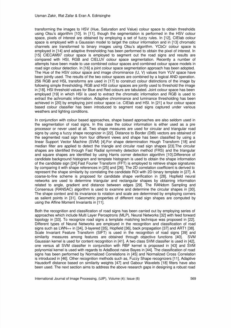
8/6/2019 International Journal of Image Processing (IJIP) Volume 4 Issue 6
http://slidepdf.com/reader/full/international-journal-of-image-processing-ijip-volume-4-issue-6 60/172
Usman Zakir, Iffat Zafar & Eran A. Edirisinghe
International Journal of Image Processing, (IJIP), Volume (4): Issue (6) 569
transforming the images to HSV (Hue, Saturation and Value) colour space to obtain thresholdsusing Otsu’s algorithm [10]. In [11], though the segmentation is performed in the HSV colourspace, pixels of interest are obtained by employing a set of fuzzy rules. In [12], CIElab colourspace is employed with a Gaussian model to target the colour information and in [13] chromaticchannels are transformed to binary images using Otsu’s algorithm. YCbCr colour space isemployed in [14] and adaptive thresholding has been performed to obtain the pixel of interest. In[15] CIECAM97 colour space is employed to segment out the road signs and results arecompared with HSI, RGB and CIELUV colour space segmentation. Recently a number ofattempts have been made to use combined colour spaces and combined colour space models inroad sign colour detection. In [16] a joint colour space segmentation approach has been adopted.The Hue of the HSV colour space and image chrominance (U, V) values from YUV space havebeen jointly used. The results of the two colour spaces are combined by a logical AND operation.256 RGB and HSL transforms are used in [17] to construct colour distinctions of the image byfollowing simple thresholding. RGB and HSI colour spaces are jointly used to threshold the imagein [18]. HSI threshold values for Blue and Red colours are tabulated. Joint colour space has beenemployed [19] in which HSI is used to extract the chromatic information and RGB is used toextract the achromatic information. Adaptive chrominance and luminance thresholding has beenachieved in [20] by employing joint colour space i.e. CIElab and HSI. In [21] a four colour spacebased colour classifier has been introduced to segment road signs captured under variousweathers and lighting conditions.
In conjunction with colour based approaches, shape based approaches are also seldom used inthe segmentation of road signs. In this case the colour information is either used as a preprocessor or never used at all. Two shape measures are used for circular and triangular roadsigns by using a fuzzy shape recognizer in [22]. Distance to Border (DtB) vectors are obtained ofthe segmented road sign from four different views and shape has been classified by using alinear Support Vector Machine (SVM) [4].For shape determination Hough Transform [18] andmedian filter are applied to detect the triangle and circular road sign shapes [23].The circularshapes are identified through Fast Radial symmetry detection method (FRS) and the triangularand square shapes are identified by using Harris corner detection algorithm [10].Difference ofcandidate background histogram and template histogram is used to obtain the shape informationof the candidate sign [24].Fast Fourier Transform (FFT) is employed to retrieve shape signaturesby comparing it with shape references in [25] and [26]. The 2D correlation coefficient is derived to
represent the shape similarity by correlating the candidate ROI with 2D binary template in [27]. Acoarse-to-fine scheme is proposed for candidate shape verification in [28]. Hopfield neuralnetworks are used to determine triangular and rectangular shapes by obtaining informationrelated to angle, gradient and distance between edges [29]. The RANdom Sampling andConsensus (RANSAC) algorithm is used to examine and determine the circular shapes in [30].The shape context and its invariance to rotation and scale are determined by employing cornersas salient points in [31]. Geometric properties of different road sign shapes are computed byusing the Affine Moment Invariants in [11].
Both the recognition and classification of road signs has been carried out by employing series ofapproaches which include Multi Layer Perceptrons (MLP), Neural Networks [32] with feed forwardtopology in [33]. To recognize road signs a template matching technique was proposed in [22].Different types of Neural Networks are employed in the recognition and classification of road
signs such as LWN++ in [34], 3-layered [35], Hopfield [36], back propagation [37] and ART1 [38].Scale Invariant Feature Transform (SIFT) is used in the recognition of road signs [39] andsimilarity measures among features are obtained through objective functions [40]. SVMGaussian kernel is used for content recognition in [41]. A two class SVM classifier is used in [42],one versus all SVM classifier in conjunction with RBF kernel is proposed in [43] and SVMpolynomial kernel is used with regards to AdaBoost naive Bayes in [44]. The classification of roadsigns has been performed by Normalized Correlations in [45] and Normalized Cross Correlationis introduced in [46]. Other recognition methods such as, Fuzzy Shape recognizers [11], AdaptiveHausdorff distance based on similarity weights [47] and Gabour Wavelets [18] filters have alsobeen used. The next section aims to address the above research gaps in designing a robust road
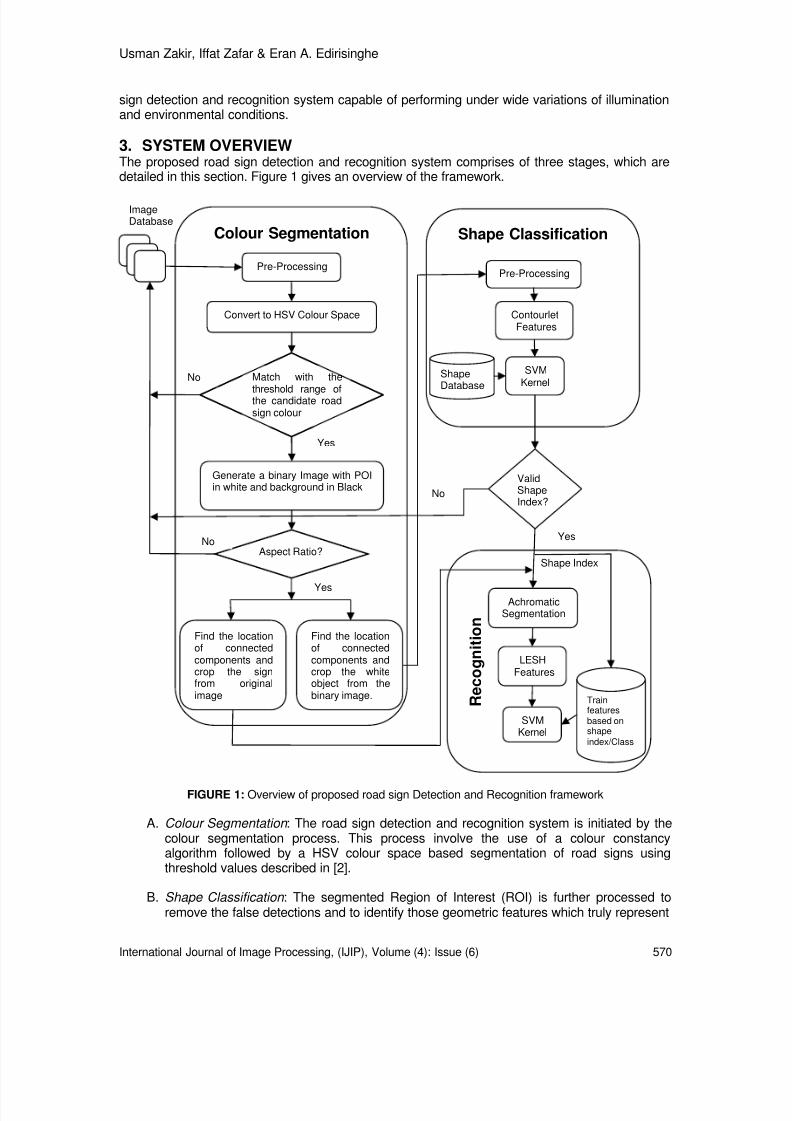
8/6/2019 International Journal of Image Processing (IJIP) Volume 4 Issue 6
http://slidepdf.com/reader/full/international-journal-of-image-processing-ijip-volume-4-issue-6 61/172

8/6/2019 International Journal of Image Processing (IJIP) Volume 4 Issue 6
http://slidepdf.com/reader/full/international-journal-of-image-processing-ijip-volume-4-issue-6 62/172
Usman Zakir, Iffat Zafar & Eran A. Edirisinghe
International Journal of Image Processing, (IJIP), Volume (4): Issue (6) 571
road signs. Contourlet Transforms with Support Vector Machine (SVM) kernel are appliedto measure the shape properties at this stage.
C. Recognition : The road signs have different meanings according to their contents. Therecognition stage comprises of the use of Local Energy based Shape Histogram featureswith SVM kernel to recognize various contents of road signs at this stage.
3.1 Colour SegmentationAs mentioned in section 2 the segmentation process of the road sign is initiated by employing acolour space. The possible challenges such as variation in illumination and exposure to rain/sunlight may affect the colour definition of the road signs. We have employed HSV colour space tosegment the colour of the road sign due to its ability to enhance segmentation results [2] ascompared to other available colour spaces, specifically in the outdoor environments. RGB imagestaken from the camera are first passed through a pre-processing stage which helps to maintainthe colour constancy in different illumination conditions [49]. It is then transformed to HSV colourspace using the following equation [48].
( ) ( )( ) ( )( )
−−+−
−+−= −
BG B RG R
B RG R H 2
1 5.0
cos (1)
( ) BG R BG R
S ,,min3
1
++−= (2)
( ) BG RV ,,max= (3)
Where R,G and B are representing the three channels of a RGB image. Pixels of interest (POI)can be segmented by using all three of the above components as shown in equation 1-3 i.e. H, Sand V. The Hue (H) component contains the colour information while Saturation(S) generatesdifferent shades of a particular colour and Value (V) indicates the brightness or darkness of thecolour components respectively. Every colour in H component of HSV colour gamut has anangular value which varies according to change appears in S and V components. If S and Vcomponents remain constant i.e. S = 100% and I = 100% then Red, Green and Blue colours canbe found at o0 , o120 and o240 anti clock wise respectively. These values are determined bytaking the histogram of H, S and V components. In the segmentation process a desired pixelwhich belongs to Red, Blue or Green colours are represented by 1 or white colour and rest of thepixels are treated as background or 0 as shown in the Figures 2(b) and 3(b). At this stage wehave to utilize a rule based approach to keep the segmentation process as fine as possible. Atfirst instance median filtering and thinning are utilized for improving the segmentationconsistency. Further to this, objects are selected as road sign candidate and discarded as noiseaccording to their aspect ratio. A priority definition of the colours is embedded with the aspectratio of the candidate sign to help in selection and rejection process which is shown in Table 2.Red colour has high priority and it can appear to be Triangle, Hexagon or Circular shape in thescene. Blue colour can appear as rectangle and circle where as Green coloured signs can appearas Rectangular shape in the image. The corresponding bounding box of the segmented object isanalyzed according to its centre and corner points as illustrated in the Figure 4. The segmentedobjects within the aspect ratio should meet this sign criteria definition. The Figure 2(c) and 3(c)are the results after removing objects with unsuitable aspect ratio and sign criteria.

8/6/2019 International Journal of Image Processing (IJIP) Volume 4 Issue 6
http://slidepdf.com/reader/full/international-journal-of-image-processing-ijip-volume-4-issue-6 63/172
Usman Zakir, Iffat Zafar & Eran A. Edirisinghe
International Journal of Image Processing, (IJIP), Volume (4): Issue (6) 572
(a) (b) (c)
FIGURE 2: Red Colour Segmentation
(a) (b) (c)
FIGURE 3: Blue Colour Segmentation
Colour Priority ShapeRed 1 Triangle, Hexagon, CircleBlue 2 Rectangle, Circle
Green 3 Rectangle
TABLE 2: Colours with their shapes and priority
FIGURE 4: The Sign Criteria
3.2 Shape ClassificationRoad Signs are represented by basic geometric shapes i.e. Triangular, Circular, Hexagonal andSquare/Rectangle. This analysis of the road sign, consisting of one of the shapes mentionedearlier is carried out after Colour Segmentation of the road signs. It not only helps to remove non-
sign objects but also lessen the burden at recognition stage.The segmented objects resulting from Colour Segmentation stage are pre-processed at the firststage of the Shape Classification. The pre-processing involves edge sharpening and filling theholes inside the objects. Figure 5 shows the procedure of pre-processing stage in the ShapeClassification where as Figure 5(b) shows processed objects which is the output of the pre-processing stage. The Contourlet Transform [50] that is successfully used in image compressionand enhancement domains has been employed here to extract the shape features of the pre-processed objects. The shape features comprises of contour edges of an object along 2dimensional (2D) spaces. These contours are stored for training or testing purposes in the later
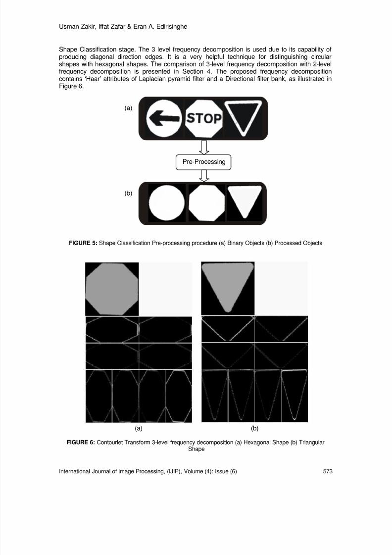
8/6/2019 International Journal of Image Processing (IJIP) Volume 4 Issue 6
http://slidepdf.com/reader/full/international-journal-of-image-processing-ijip-volume-4-issue-6 64/172
Usman Zakir, Iffat Zafar & Eran A. Edirisinghe
International Journal of Image Processing, (IJIP), Volume (4): Issue (6) 573
Shape Classification stage. The 3 level frequency decomposition is used due to its capability ofproducing diagonal direction edges. It is a very helpful technique for distinguishing circularshapes with hexagonal shapes. The comparison of 3-level frequency decomposition with 2-levelfrequency decomposition is presented in Section 4. The proposed frequency decompositioncontains ‘Haar’ attributes of Laplacian pyramid filter and a Directional filter bank, as illustrated inFigure 6.
(a)
(b)
FIGURE 5: Shape Classification Pre-processing procedure (a) Binary Objects (b) Processed Objects
(a) (b)
FIGURE 6: Contourlet Transform 3-level frequency decomposition (a) Hexagonal Shape (b) TriangularShape
Pre-Processing

8/6/2019 International Journal of Image Processing (IJIP) Volume 4 Issue 6
http://slidepdf.com/reader/full/international-journal-of-image-processing-ijip-volume-4-issue-6 65/172
Usman Zakir, Iffat Zafar & Eran A. Edirisinghe
International Journal of Image Processing, (IJIP), Volume (4): Issue (6) 574
The extracted Contourlet features of different shapes are fed in to Support Vector Machine (SVM)which helps to classify the exact shape of the candidate sign. The SVM classifier first proposed in[51] is an effective and powerful method for general purpose pattern recognition andclassification. SVM based kernels are used to map the input data to the high dimensional featurespace and process it in linear form. In our experiments we have tested few popular kernels
functions, ( )vuk , defined as follows:
( ) vuvuk ,, = (4)
( ) ( )d vuvuk 1., += (5)
( ) 2
2
, σ
vu
evuk
−
=
(6)
In most applications it has been generally concluded that, a low degree polynomial kernel shownin equation (5) or a Radial Basis Function (RBF) as kernel shown in equation (6) works quite well.In our case, a polynomial kernel with degree 1 and 2 provides the best results for shapeclassification. The method described here for shape classification is invariant to scale, rotation
and partial occlusion problems. The method has the capability to classify any geometric shapedue to its distinguishing multi channels feature analysis.
3.3 RecognitionOnce the candidate shape is classified, it initiates the process of Recognition and classification ofthe road sign contents. The Recognition process comprises of the LESH features extraction ofthe road sign contents and training/testing of these features is carried out by employing SVMkernel classifier. The candidate road signs which are extracted through Colour Segmentation andhence validated as the road sign shape by Shape Classification are further processed to obtainthe valid road sign contents for feature extraction.
The road sign contents are normally represented with black and white colours. In this contextachromatic segmentation is introduced to extract the black and white areas of the candidate road
sign from rest of the image. The objects which are meeting the criteria of aspect ratio areconsidered as valid road sign contents and vice versa. The black and white objects afterachromatic segmentation and in accordance to aspect ratio are shown in Figure 7.
(a) (b) (c) (d) (e)
FIGURE 7: Road signs after achromatic segmentation
The Local Energy Model was first introduced in [52] proving that features can be extracted atthose points from an image where local frequency components represent maximum uniformity.The extended framework of local energy model is given in Equation (8) and is normalized by thesummation of noise cancellation factor T , Sine of phase deviation and factor W , which is theweighting of the frequency spread. Further details of this extended framework can be found in[53].

8/6/2019 International Journal of Image Processing (IJIP) Volume 4 Issue 6
http://slidepdf.com/reader/full/international-journal-of-image-processing-ijip-volume-4-issue-6 66/172
Usman Zakir, Iffat Zafar & Eran A. Edirisinghe
International Journal of Image Processing, (IJIP), Volume (4): Issue (6) 575
( ) ( ) ( ) ( )( ) ( ) ( )( )( ) ε
φ φ φ φ +
−−−−=
∑∑
n n
n nnn
x A
T x x x x x A xW E
sincos
(8)
The Local Energy gives reliable information to extract the interest points from an image in aninvariant manner to illumination and noise. This raw energy indicates the corners, contours oredges of underlying shape in an image. LESH [54] features are obtained firstly by dividing thecandidate image into 16 sub-regions and then the local energy information is calculated for eachsub-region along 8 different orientations with the help of Gabor Wavelets kernels [55].
( ) ( ) ( ) z z I zG vuvu ,,Ψ∗= (9)
Where ( ) y x z ,= represents the image position, the symbol “ ∗” is convolution operator and
( ) zvu ,Ψ can be calculated as equation (10).
( ) −=Ψ −
−
22
,2
2
22,
2
2
,,
σ σ
σ eeek z zvuik
zvuk
vuvu (10)
The orientation label map is produced representing labels of orientation of pixels containinglargest energy across all scales in an image. The local histogram h is calculated in equation (12)as follows:
( ) ( )2
22
2
1 σ
πσ
−+−
=
yor y xor x
r ew (11)
Lbr br E wh δ ××= ∑, (12)
Where w is the Gaussian weighting function of region r calculated as in equation (11), E represents the local energy computed as equation (8), Lbδ represents Kronecker’s delta, L
orientation label map and b current bin. From the above description it can be seen that the LESHdescriptor of a shape is 8x16=128 dimensional feature vector.
Each object shown in Figure 7(a-e) is representing a separate class of objects. These objects arenormalized into fixed size dimensions and converted to gray level images. The next stage is toextract the LESH features of these normalized images. LESH features are obtained by computingthe local energy along each filter orientation of image sub-region and its histogram is generated.The overall histogram represents the concatenated histograms computed along each sub-regionof the image. Figure 8 shows the LESH features representation of 30 speed limit and round aboutsigns respectively. These features from different classes are classified with the help of multiclass
SVM polynomial kernel which is explained earlier in section 3.2.
4. EXPERIMENTAL SETUP AND RESULTSUsing a standard photographic camera, mounted of a car, we have obtained 1200 images ofdifferent road signs. These signs were captured during various ambient and lit-up levels ofillumination and weather conditions. The road signs collected were limited to ones with basiccolours i.e. Red, Green and Blue. Figure 9 illustrates some samples of images taken from aCanon IXUS80IS digital camera at a resolution of 2592 x 1944. The images are pre-processedbefore converting them to the HSV colour space. This involves the stabilization process of colour
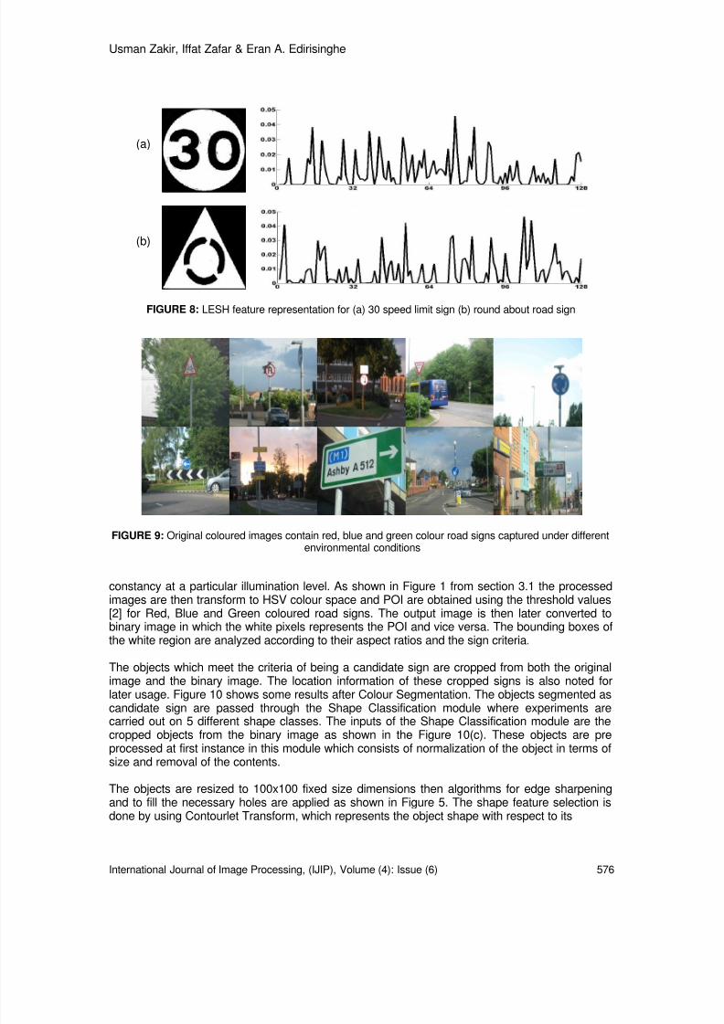
8/6/2019 International Journal of Image Processing (IJIP) Volume 4 Issue 6
http://slidepdf.com/reader/full/international-journal-of-image-processing-ijip-volume-4-issue-6 67/172
Usman Zakir, Iffat Zafar & Eran A. Edirisinghe
International Journal of Image Processing, (IJIP), Volume (4): Issue (6) 576
FIGURE 8: LESH feature representation for (a) 30 speed limit sign (b) round about road sign
FIGURE 9: Original coloured images contain red, blue and green colour road signs captured under differentenvironmental conditions
constancy at a particular illumination level. As shown in Figure 1 from section 3.1 the processedimages are then transform to HSV colour space and POI are obtained using the threshold values[2] for Red, Blue and Green coloured road signs. The output image is then later converted tobinary image in which the white pixels represents the POI and vice versa. The bounding boxes ofthe white region are analyzed according to their aspect ratios and the sign criteria.
The objects which meet the criteria of being a candidate sign are cropped from both the originalimage and the binary image. The location information of these cropped signs is also noted forlater usage. Figure 10 shows some results after Colour Segmentation. The objects segmented ascandidate sign are passed through the Shape Classification module where experiments arecarried out on 5 different shape classes. The inputs of the Shape Classification module are thecropped objects from the binary image as shown in the Figure 10(c). These objects are preprocessed at first instance in this module which consists of normalization of the object in terms ofsize and removal of the contents.
The objects are resized to 100x100 fixed size dimensions then algorithms for edge sharpeningand to fill the necessary holes are applied as shown in Figure 5. The shape feature selection isdone by using Contourlet Transform, which represents the object shape with respect to its
(a)
(b)

8/6/2019 International Journal of Image Processing (IJIP) Volume 4 Issue 6
http://slidepdf.com/reader/full/international-journal-of-image-processing-ijip-volume-4-issue-6 68/172
Usman Zakir, Iffat Zafar & Eran A. Edirisinghe
International Journal of Image Processing, (IJIP), Volume (4): Issue (6) 577
FIGURE 10: Colour Segmentation using HSV colour space (a) Road Signs in the natural environment (b)Cropped Road Signs from the original Image (c) Cropped Road Signs from the Binary Image
Index Shape Level* Pyramidal andDirectional Filters
TrainedInstances
1 3 Haar 502 3 Haar 503 3 Haar 504 3 Haar 505 3 Haar 50
TABLE 3: Shapes considered for obtaining Contourlet features, Level* = Sub band Decomposition
ShapeIndex
Classified Shapes with LevelLevel Success Level Success
1 2 75% 3 100%2 2 0% 3 100%3 2 75% 3 100%4 2 100% 3 100%5 2 100% 3 100%
TABLE 4: Success percentage at different decomposition Levels
(a) (b) (c)
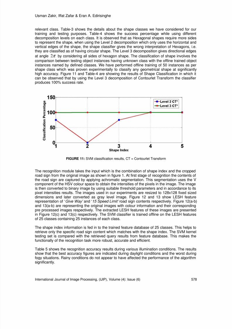
8/6/2019 International Journal of Image Processing (IJIP) Volume 4 Issue 6
http://slidepdf.com/reader/full/international-journal-of-image-processing-ijip-volume-4-issue-6 69/172
Usman Zakir, Iffat Zafar & Eran A. Edirisinghe
International Journal of Image Processing, (IJIP), Volume (4): Issue (6) 578
relevant class. Table-3 shows the details about the shape classes we have considered for ourtraining and testing purposes. Table-4 shows the success percentage while using differentdecomposition levels on each class. It is observed that as Hexagonal shapes require more sidesto represent the shape, when using the Level 2 decomposition which only uses the horizontal andvertical edges of the shape, the shape classifier gives the wrong interpretation of Hexagons, i.e.they are classified as of having circular shape. The Level 3 decomposition gives directional edges
at angle π 2 by considering all sides of hexagon shape. The classification of shape involves thecomparison between testing object instances having unknown class with the offline trained objectinstances named by defined classes. We have performed offline training of 50 instances as pershape class which was proven experimentally to classify any geometrical shape at significantlyhigh accuracy. Figure 11 and Table-4 are showing the results of Shape Classification in which itcan be observed that by using the Level 3 decomposition of Contourlet Transform the classifierproduces 100% success rate.
FIGURE 11: SVM classification results, CT = Contourlet Transform
The recognition module takes the input which is the combination of shape index and the croppedroad sign from the original image as shown in figure 1. At first stage of recognition the contents ofthe road sign are captured by applying achromatic segmentation. This segmentation uses the Vcomponent of the HSV colour space to obtain the intensities of the pixels in the image. The imageis then converted to binary image by using suitable threshold parameters and in accordance to itspixel intensities results. The images used in our experiments are resized to 128x128 fixed sizeddimensions and later converted as gray level image. Figure 12 and 13 show LESH featurerepresentation of ‘ Give Way’ and ‘ 15 Speed Limit’ road sign contents respectively. Figure 12(a-b)and 13(a-b) are representing the original images with colour information and their correspondingpre processed images respectively. The extracted LESH features of these images are presentedin Figure 12(c) and 13(c) respectively. The SVM classifier is trained offline on the LESH featuresof 25 classes containing 25 instances of each class.
The shape index information is fed in to the trained feature database of 25 classes. This helps toretrieve only the specific road sign content which matches with the shape index. The SVM kerneltesting set is compared with the retrieved query results from feature database. This makes thefunctionally of the recognition task more robust, accurate and efficient.
Table 5 shows the recognition accuracy results during various illumination conditions. The resultsshow that the best accuracy figures are indicated during daylight conditions and the worst duringfogy situations. Rainy conditions do not appear to have affected the performance of the algorithmsignificantly.
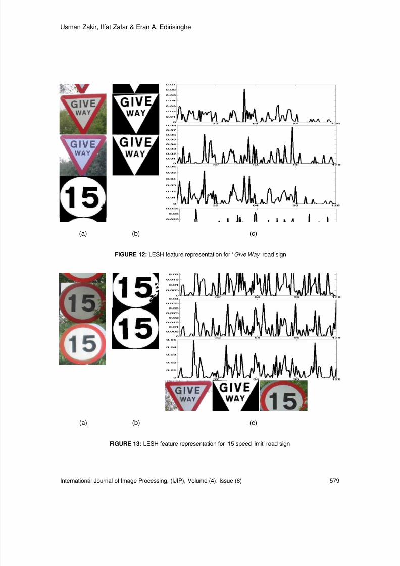
8/6/2019 International Journal of Image Processing (IJIP) Volume 4 Issue 6
http://slidepdf.com/reader/full/international-journal-of-image-processing-ijip-volume-4-issue-6 70/172
Usman Zakir, Iffat Zafar & Eran A. Edirisinghe
International Journal of Image Processing, (IJIP), Volume (4): Issue (6) 579
(a) (b) (c)
FIGURE 12: LESH feature representation for ‘ Give Way’ road sign
(a) (b) (c)
FIGURE 13: LESH feature representation for ‘15 speed limit’ road sign

8/6/2019 International Journal of Image Processing (IJIP) Volume 4 Issue 6
http://slidepdf.com/reader/full/international-journal-of-image-processing-ijip-volume-4-issue-6 71/172
Usman Zakir, Iffat Zafar & Eran A. Edirisinghe
International Journal of Image Processing, (IJIP), Volume (4): Issue (6) 580
Ambient IlluminationDay light Raining Fog Night
Traffic Signs 560 430 70 110Correct Recognition 552 426 61 103
False Recognition 8 4 9 7TABLE 5: Recognition results during various levels of ambient illumination
5. CONSLUSION & FUTURE WORKIn this paper we have presented a novel approach towards road sign detection and recognition.The system utilizes a robust method of Colour Segmentation by employing the HSV colour spaceand using empirically determined threshold values suitable for various illumination conditions. Anovel Shape Classification methodology is proposed in which all possible road sign shapes areclassified by introducing the use of Contourlet Transform with SVM classifier. The Recognition stage introduces the SVM classifier with the Local Energy based Shape Histogram (LESH)features. We have provided experimental results to prove the effectiveness of this approachunder varying levels of illumination and environmental conditions. Overall accuracy figures of 96-98% have been reported. We are currently working on real time application of the algorithm withinan in-car navigation system.
6. REFERENCES1. S. M. Bascón, S. L. Arroyo, P. G. Jiménez, H. G. Moreno and F. L. Ferreras. “Road-Sign
Detection and Recognition Based on Support Vector Machines”. IEEE Transactions onIntelligent Transportation Systems, 8(2):264-278, 2007
2. U. Zakir, A. N. J. Leonce and E. A. Edirisinghe. “Road sign segmentation based on colour spaces: A Comparative Study”. In Proceedings of the 11th Iasted International Conference onComputer Graphics and Imgaing, Innsbruck, Austria, 2010
3. Y.Y. Nguwi and S.Y. Cho. “Two-tier Self-Organizing Visual Model for Road Sign Recognition”.International Joint Conference on Neural Networks, IJCNN, 2008
4. Y.Y. Nguwi and A.Z. Kouzani. “Detection and classification of road signs in natural environments” . Neural Computing & Applications, 265–289, 2008
5. V.Andrey and K.H.Jo. “Automatic Detection and Recognition of Traffic Signs using Geometric Structure Analysis” . SICE-ICASE International Joint Conference, Korea, 2006
6. J. Wu and Y. Tsai. “Enhanced Roadway Inventory Using a 2-D Sign Video Image Recognition Algorithm”. Computer-Aided Civil and Infrastructure Engineering, 369–382, 2006
7. M. Benallal and J. Meunier. “Real-time colour segmentation of road signs". CanadianConference on Electrical and Computer Engineering, 2003.
8. P. Medici, C. Caraffi, E. Cardarelli and P.P. Porta. “Real Time Road Signs Classification”. Proceedings of the IEEE International Conference on Vehicular Electronics and SafetyColumbus, USA., 2008
9. W.Y. Wu, T.C. Hsieh and C.S. Lai. “Extracting Road Signs using the Color Information”, WorldAcademy of Science, Engineering and Technology, 32, 2007.

8/6/2019 International Journal of Image Processing (IJIP) Volume 4 Issue 6
http://slidepdf.com/reader/full/international-journal-of-image-processing-ijip-volume-4-issue-6 72/172
Usman Zakir, Iffat Zafar & Eran A. Edirisinghe
International Journal of Image Processing, (IJIP), Volume (4): Issue (6) 581
10. C.F. Paulo and P.L. Correia. “Automatic Detection and Classification of Traffic Signs”. EighthInternational Workshop on Image Analysis for Multimedia Int, Services, Greece, 2007
11. H. Fleyeh. “Traffic Sign Recognition by Fuzzy Sets”. IEEE Intelligent Vehicles SymposiumEindhoven University of Technology Eindhoven, Netherlands, 2008
12. L. D. Lopez and O. Fuentes. “Colour-Based Road Sign Detection and Tracking”. Springer,Lecture Notes in Computer Science, 2007
13. G.K. Siogkas and E.S. Dermatas, Detection. “Tracking and Classification of Road Signs in Adverse Conditions”. IEEE Mediterranean Electrotechnical Conference, MELECON, 2006
14. M.L. Eichner and T.P. Breckon. “Integrated Speed Limit Detection and Recognition from Real- Time Video”. In Proceedings of IEEE Intelligent Vehicles Symposium ,2008
15. X. Gao, K. Hong, P. Passmore, L. Podladchikova and D.Shaposhnikov. “Colour Vision Model- Based Approach for Segmentation of Traffic Signs”. EURASIP Journal on Image and VideoProcessing, 2008.
16. W. G. Shadeed, D. I. Abu-Al-Nadi, and M. J. Mismar. “Road traffic sign detection in color images”. In Proceedings of the 10th IEEE International Conference on Electronics, Circuitsand Systems, 2003
17. D. Matsuura, H. Yamauchi and H. Takahashi. “Extracting Circular Road Signs Using Specific Color Distinction and Region Limitation”. Systems and Computers in Japan, 2007
18. H. Huang, C. Chen, Y. Jia and S. Tang. “Automatic Detection and Recognition of Circular Road Sign”. IEEE/ASME International Conference on Mechtronic and Embedded Systemsand Applications, MESA, 2008
19. N. Bose, M. Shirvaikar and R. Pieper. “A Real Time Automatic Sign Interpretation System for Operator Assistance”. Proceedings of the 38th Southeastern Symp on System TheoryTennessee Technological Univ. Cookeville, TN, USA, 2006
20. A. V. Reina, R. Sastre, S. Arroyo and P. Jimenez. “Adaptive traffic road sign panels text extraction”. Proceedings of the 5th WSEAS International conference on Signal Processing,Robotics and Automation, Madrid, Spain, 2006
21. U. Zakir, I. Zafar, E. A. Edirisinghe. “A Novel Approach to In-Car Road Sign Recognition”. The14th International Conference on Machine Design and Production, Cyprus 2010
22. R. Malik,J. Khurshid and S.N. Ahmad. “Road Sign Detection and Recognition using colour segmentation, Shape analysis and Template Matching”. Proceedings of the Sixth InternationalConference on Machine Learning and Cybernetics, Hong Kong, 2007
23. W.J. Kuo and C.C. Lin. “Two- Stage Road Sign Detection and Recognition” . IEEE
International Conference on Multimedia and Expo, 200724. V.Andrey and K.H.Jo. “Automatic Detection and Recognition of Traffic Signs using
Geometric Structure Analysis” . SICE-ICASE International Joint Conference, Korea, 2006
25. A. V. Reina, R. J. L. Sastre, S. L. Arroyo and P.G. Jimenez. “Adaptive traffic road sign panels text extraction”. Proceedings of the 5th WSEAS International Conference on SignalProcessing, Robotics and Automation, Madrid, Spain, 2006

8/6/2019 International Journal of Image Processing (IJIP) Volume 4 Issue 6
http://slidepdf.com/reader/full/international-journal-of-image-processing-ijip-volume-4-issue-6 73/172
Usman Zakir, Iffat Zafar & Eran A. Edirisinghe
International Journal of Image Processing, (IJIP), Volume (4): Issue (6) 582
26. P. Gil-Jim´enez, S. Lafuente-Arroyo, H. G´omez-Moreno, F. L´opez-Ferreras and S.Maldonado-Basc´on. “Traffic sign shape classification evaluation II: FFT applied to the signature of Blobs”. 607- 612 ,2005
27. J. Wu and Y. Tsai. “Enhanced Roadway Inventory Using a 2-D Sign Video Image Recognition Algorithm”. Computer-Aided Civil and Infrastructure Engineering, 21: 2006, 369–382
28. L.W. Tsai, J.W. Hsieh, C.H. Chuang, Y.J. Tseng, K.C. Fan, C.C. Lee. “Road sign detection using eigen colour”. IET Computer Vision 2(3): 164–177, 2008
29. G.H. Kim, H.G. Sohn and Y.S. Song. ”Road Infrastructure Data Acquisition Using a Vehicle- Based Mobile Mapping System”. Computer-Aided Civil and Infrastructure Engineering, 2(1):346–356, 2006
30. M.L. Eichner and T.P. Breckon. “Integrated Speed Limit Detection and Recognition from Real- Time Video”. In Proceedings of IEEE Intelligent Vehicles Symposium, 2008
31. P. Silapachote and A. H. R. Weiss. “A Hierarchical Approach to Sign Recognition”. Proceedings of the Seventh IEEE Workshop on Applications of Computer Vision,2005
32. Y. Y. Nguwi and A. Z. Kouzani. “Detection and classification of road signs in natural environments”. Neural Computing & Applications, 17: 265–289, 2008
33. P. Medici, C. Caraffi., E. Cardarelli and P. P. Porta. “Real Time Road Signs Classification”. Proceedings of the IEEE International Conference on Vehicular Electronics and SafetyColumbus, USA, 2008
34. A. Broggi, P. Cerri, P. Medici, P. P. Porta. “Real Time Road Signs Recognition”. Proceedingsof the IEEE Intelligent Vehicles Symposium Istanbul, Turkey, 2007
35. H. Ohara, I. Nishikawa, S. Miki, N. Yabuki. “Detection and Recognition of Road Signs using simple layered Neural Networks”. Proceedings of the 9th International Conference on NeuralInformation Processing, 2002
36. G. H. Kim, H. G. Sohn and Y. S. Song. “Road Infrastructure Data Acquisition Using a Vehicle- Based Mobile Mapping System”. Computer-Aided Civil and Infrastructure Engineering, 21:346–356, 2006
37. N. Kehtarnavaz, A. Ahmad. “Traffic Sign Recognition in Noisy Outdoor Scenes”. IEEE,Intelligent Vehicles. 1995
38. A. D. L. Escalera., J. M. Armingol and M. Mata. “Traffic sign recognition and analysis for intelligent vehicles”. Image and Vision Computing, 21: 247–258, 2003
39. A. A. Farag and A. E. Abdel-Hakim. “Detection, Categorization and Recognition of Road Signs for Autonomous Navigation”. Proceedings of Acivs (Advanced Concepts for Intelligent Vision
Systems), Brussels, Belgium, 200440. W. G. Shadeed, D. I. Abu-Al-Nadi, and M. J. Mismar. “Road traffic sign detection in color
images”. In Proceedings of the 10th IEEE International Conference on Electronics, Circuitsand Systems, 2: 890–893,2003
41. S. Lafuente-Arroyo, S. Maldonado-Bascon, P. Gil-Jimenez, J. Acevedo- Rodriguez, and R.Lopez-Sastre. ”A tracking system for automated inventory of road signs”. IEEE IntelligentVehicles Symposium,166-171, 2007

8/6/2019 International Journal of Image Processing (IJIP) Volume 4 Issue 6
http://slidepdf.com/reader/full/international-journal-of-image-processing-ijip-volume-4-issue-6 74/172

8/6/2019 International Journal of Image Processing (IJIP) Volume 4 Issue 6
http://slidepdf.com/reader/full/international-journal-of-image-processing-ijip-volume-4-issue-6 75/172
Jack Collins, Christopher Kurcz, Curtis Lisle, Yanling Liu & Enrique Zudaire
International Journal of Image Processing, (IJIP), Volume (4): Issue (6) 584
Assessment of Vascular Network Segmentation
Jack Collins [email protected], Inc., NCI-Frederick
Frederick, 21702, USA
Christopher Kurcz [email protected], Inc., NCI-Frederick Frederick, 21702, USA
Curtis Lisle [email protected] LLC Maitland, 32751, USA
Yanling Liu [email protected], Inc., NCI-Frederick
Frederick, 21702, USA Enrique Zudaire [email protected] Core Facility, NCI NIHGaithersburg, 20877, USA
Abstract
We present an analysis framework to assess the quality and accuracy of vesselsegmentation algorithms for three dimensional images. We generate synthetic (insilico) vessel models which act as ground truth and are constructed to embodyvarying morphological features. These models are transformed into imagesconstructed under different levels of contrast, noise, and intensity. Todemonstrate the use of our framework, we implemented two segmentationalgorithms and compare the results to the ground truth model using severalmeasures to quantify the accuracy and quality of segmentation. Furthermore, wecollect metrics which describe the characteristics of the vessels it fails tosegment. Our approach is illustrated with several examples. Funded by NCIContract No.HHSN261200800001E.
Keywords: Vessel Segmentation, Network Comparison, Quantitative Analysis, Segmentation Quality,Segmentation Accuracy.
1. INTRODUCTION Extracting vascular networks from three dimensional images remains a difficult and excitingchallenge. Many segmentation algorithms have been designed to target different types ofvasculature imaged using various modalities and are applied to a wide range of problems indisease diagnosis, flow dynamics, surgical planning, etc... (see e.g. [2][1][3]). Despite thesophistication of these methods, it is often difficult to choose a particular segmentation algorithmgiven a collection of similar images since a given method may make implicit assumptions aboutimage or vessel characteristics. Furthermore, it is not clear how to predict or quantify the qualityor accuracy of a given method onthose images due to a lack of ground truth data.

8/6/2019 International Journal of Image Processing (IJIP) Volume 4 Issue 6
http://slidepdf.com/reader/full/international-journal-of-image-processing-ijip-volume-4-issue-6 76/172
Jack Collins, Christopher Kurcz, Curtis Lisle, Yanling Liu & Enrique Zudaire
International Journal of Image Processing, (IJIP), Volume (4): Issue (6) 585
In this paper, we provide a methodology to quantify the accuracy and effectiveness of a vesselsegmentation algorithm. We provide tools for constructing a model vessel tree which defines thevessel centerline locations and vessel radius and serves as ground truth. This model istransformed into an image with specified contrast, noise and intensity profile and serves as inputto the segmentation algorithm under scrutiny. At a minimum we require the segmentationalgorithm to produce a binary image depicting vessel location. Additional data including vesselradius, curvature, and local coordinate system may also be specified. This data is thentransformed into a graph (network) representation and aligned with the model tree to determinethe quality and accuracy of segmentation. We illustrate these operations in Figure 1.
We emphasize that our approach quantifies segmentation quality and accuracy by comparingattribute graphs and not images. By using the model vessel tree as a starting point and simulatingthe imaging process we can assess the performance of a segmentation algorithm under a varietyof image characteristics. Furthermore, we do not require a trained observer to extract thecenterlines from a gold standard data set since the model vessel tree contains centerline locationas an attribute. Morphological features (e.g. vessel radius, curvature, tortuosity, etc...) aremaintained as attributes of the model vessel tree and we can assess the segmentationperformance as a function of these features.
We provide metrics describing the correctly segmented vessels, missed vessels, false positivesand changes in network topology to assess segmentation quality. Beyond the qualityassessment, we determine the accuracy of segmentation by computing the deviation of thecenterline and radius between the ground truth model and the segmentation estimation.Additional assessment includes collecting features where that algorithm fails (e.g. did thealgorithm fail to detect thin or highly curvedvessels?). Thus, we provide a framework to determinehow well a particular segmentation algorithm performs as a function of the image quality definedby contrast, noise, and intensity profile. This paper is organized as follows. In Section 2, wedescribe the model tree creation, transformation of the model tree to an image, segmentation ofthe image, and comparison of the segmented result to the model. Next, in Section 3, we performa quality and accuracy assessment for several models. Finally, in Section 4, we summarize theresults for the different models and describe possible extensions and improvements to ourapproach.
FIGURE 1: Flow Chart of Major Operations in Vessel Segmentation Assessment Framework
2. MATERIALS AND METHODS In this section we describe the process of model vessel tree generation, model tree to imageformation, segmentation of vessels from a noise corrupted image, and a method to compare themodel to the segmentation result.
2.1 Model Tree GenerationWe construct model vessel trees which serve as ground truth for subsequent analysis.Lindenmayer systems [17][18] ( L-systems) provide a natural framework for defining such objects.This formalism grows a tree from a root location by following a set of rules which specify thedirection of growth, branch radius, branch length, angle between branches and number ofbranches. In Figure 2 we illustrate this procedure with a simple example. We note that L-systemshave been used in a variety of applications in computational botany, computer graphics, andmedicine (see e.g. [10][24][20][21]). Although our model is formally a tree, there is nofundamental limitation for its extension to a more complicated topology.
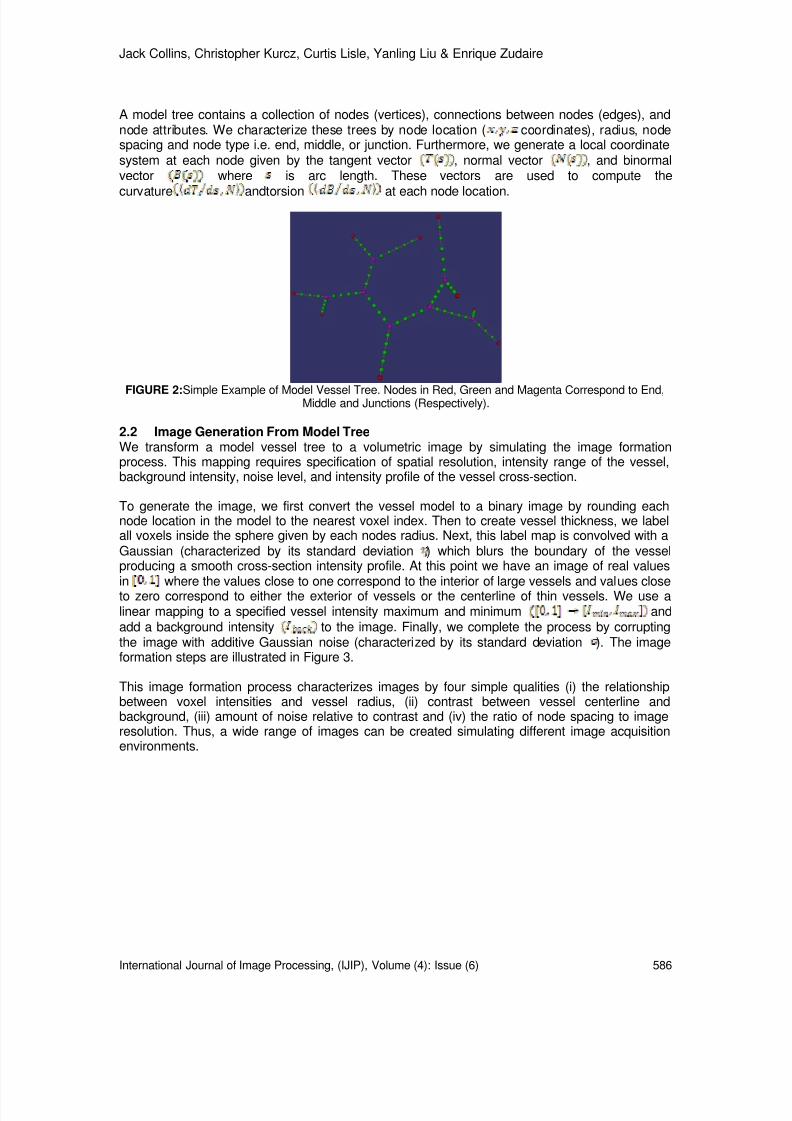
8/6/2019 International Journal of Image Processing (IJIP) Volume 4 Issue 6
http://slidepdf.com/reader/full/international-journal-of-image-processing-ijip-volume-4-issue-6 77/172
Jack Collins, Christopher Kurcz, Curtis Lisle, Yanling Liu & Enrique Zudaire
International Journal of Image Processing, (IJIP), Volume (4): Issue (6) 586
A model tree contains a collection of nodes (vertices), connections between nodes (edges), andnode attributes. We characterize these trees by node location ( coordinates), radius, nodespacing and node type i.e. end, middle, or junction. Furthermore, we generate a local coordinatesystem at each node given by the tangent vector , normal vector , and binormalvector where is arc length. These vectors are used to compute the
curvature andtorsion at each node location.
FIGURE 2: Simple Example of Model Vessel Tree. Nodes in Red, Green and Magenta Correspond to End,Middle and Junctions (Respectively).
2.2 Image Generation From Model TreeWe transform a model vessel tree to a volumetric image by simulating the image formationprocess. This mapping requires specification of spatial resolution, intensity range of the vessel,background intensity, noise level, and intensity profile of the vessel cross-section.
To generate the image, we first convert the vessel model to a binary image by rounding eachnode location in the model to the nearest voxel index. Then to create vessel thickness, we labelall voxels inside the sphere given by each nodes radius. Next, this label map is convolved with aGaussian (characterized by its standard deviation ) which blurs the boundary of the vesselproducing a smooth cross-section intensity profile. At this point we have an image of real valuesin where the values close to one correspond to the interior of large vessels and values closeto zero correspond to either the exterior of vessels or the centerline of thin vessels. We use alinear mapping to a specified vessel intensity maximum and minimum andadd a background intensity to the image. Finally, we complete the process by corruptingthe image with additive Gaussian noise (characterized by its standard deviation ). The imageformation steps are illustrated in Figure 3.
This image formation process characterizes images by four simple qualities (i) the relationshipbetween voxel intensities and vessel radius, (ii) contrast between vessel centerline andbackground, (iii) amount of noise relative to contrast and (iv) the ratio of node spacing to imageresolution. Thus, a wide range of images can be created simulating different image acquisitionenvironments.

8/6/2019 International Journal of Image Processing (IJIP) Volume 4 Issue 6
http://slidepdf.com/reader/full/international-journal-of-image-processing-ijip-volume-4-issue-6 78/172
Jack Collins, Christopher Kurcz, Curtis Lisle, Yanling Liu & Enrique Zudaire
International Journal of Image Processing, (IJIP), Volume (4): Issue (6) 587
(a)
(b) (c) (d)FIGURE 3: Image Formation Process. (a) Generated Slices of Label Map Overlayed on Model Tree.For Visualization Purposes The Model Has Been Made Artificially Thinner. (b) A Slice From The Label Map.
(c) Slice From (b) After Gaussian Smoothing Intensity Rescaling andBackground Added . (d) Slice From (c) After Addition of Gaussian Noise .
2.3 Vessel SegmentationThere is a vast amount of literature and wide range of methods for vessel segmentation (seee.g.[13][19] for a review). We emphasize that the main point of this paper is not the developmentof vessel segmentation algorithms but the assessment of their performance. Toward this end, weimplemented two vessel segmentation algorithms for demonstration purposes. In what follows,we denote the image intensity at position .
2.3.1 VesselnessThe first segmentation method assumes a cylindrical model for vessels and uses the eigenvaluesof the Hessian matrix to enhance vessel voxels (see e.g. [7][25]). We begin by considering thevoxels above a specified threshold . For each specified scale, , we form theHessian matrix
(2.1)
where , * denotes the convolution operator, and denotes thepartial derivative with respect to . The eigenvalues of (2.1) are computed and ordered so that
. For each scale, we compute
(2.2)

8/6/2019 International Journal of Image Processing (IJIP) Volume 4 Issue 6
http://slidepdf.com/reader/full/international-journal-of-image-processing-ijip-volume-4-issue-6 79/172
Jack Collins, Christopher Kurcz, Curtis Lisle, Yanling Liu & Enrique Zudaire
International Journal of Image Processing, (IJIP), Volume (4): Issue (6) 588
where and . Finally, we determine the
vesselness, , and construct a label map, , by considering thevoxels above a specified vesselness threshold, .
2.3.2 Fast Marching
The second segmentation method uses the Fast Marching method (see e.g. [27][12, §9.3.1]).This method propagates an outward moving front satisfying(2.3)
from an initial surface given a speed . The solution, , to (2.3) represents the arrival time atlocation . We use a sigmoidal speed function,
where is the average intensity over a neighborhood. To construct the label map,, we consider all voxels whose arrival time is less than a specified threshold,
.
2.3.3 Post ProcessingTo aid subsequent analysis we apply the hole filling algorithm [12, §6.6.4] to the label mapconstructed from either segmentation algorithm ( ). We determine the vessel centerlineusing the skeletonization algorithm [9] and the vessel radius at each centerline location using thedistance transform [31].
From the labeled centerline image we generate a data structure which contains the locations ofthe vessel centerline at each point and refer to this structure as the segmentation graph throughout the rest of this paper. We note that its topology may deviate from a tree due tosegmentation errors. The segmentation graph is constructed by converting each centerline voxelto a node in the segmentation graph where the node location is given by the voxels physicalcoordinates. The remaining attributes of the graph are then populated. Since the model has beendiscretized during the image formation process, the node locations in the segmentation graphmay not align with those from the model. In Figure 4 we provide an example, where the spacingbetween points in the model is 1 but, the spacing between points in the segmentation graph is
either 1, or .
FIGURE4: Model Tree in Red and Segmentation Graph in Green

8/6/2019 International Journal of Image Processing (IJIP) Volume 4 Issue 6
http://slidepdf.com/reader/full/international-journal-of-image-processing-ijip-volume-4-issue-6 80/172
Jack Collins, Christopher Kurcz, Curtis Lisle, Yanling Liu & Enrique Zudaire
International Journal of Image Processing, (IJIP), Volume (4): Issue (6) 589
2.4 Graph MatchingGiven a model tree and a segmentation graph we determine the nodes in the segmentation graphthat correspond to these in the model tree. This mapping allows us to compare results ofsegmentation to ground truth. Since the spacing between nodes in the model tree and vesselgraph may differ, we use a many-to-one mapping between nodes in the segmentation graph tonodes in the model tree.
This association problem is often referred to as inexact graph matching (see e.g. [4][6][30][32])which is often posed as a global alignment problem or largest subgraph isomorphism problem.However, the problem presented here is slightly different because we have node attributeinformation which can be used to assist in the association problem. Thus, we seek a methodwhich optimizes the global alignment while minimizing the pairwise distance between nodes inthe model tree and segmentation graph.
For this purpose, we use the IsoRank algorithm [28] which constructs a set of constraints for allpairs of nodes in the model tree and segmentation graph based on neighborhood information.Using these constraints and minimizing the pairwise distances, the IsoRank algorithm establishesa ranking between pairs of nodes in the model tree and segmentation graph. We note that therankings are computed by solving for the largest eigenvalue of a sparse matrix and the entries ofthe eigenvector correspond to the pairwise ranks (as in the PageRank algorithm see e.g. [16]).The ranking matrix in combination with a maximum allowable deviation between node positionsand maximum number of multiple matches is uses to determine the many-to-one mappingbetween nodes in the segmentation graph to nodes in the model tree. An example matching isillustrated in Figure 5.
Given the association between nodes in the model tree and segmentation graph we classifynodes in the segmentation graph as either matched, missed or false positives. A matched node inthe segmentation graph is associated with one node in the model tree, a missed node in themodel tree has no association with a node in the segmentation graph and a false positive is anode in the segmentation graph with no association to a node in the model tree. Notice in Figure5 thatin a limited number of cases the algorithm can fail to match nodes that appear tocorrespond to a node in the model tree. We note that this occurs due to our enforcement of amany-to-one mapping. Adopting a many-to-many matching policy would reduce the number of
false positives at the cost of matching nodes that may not correspond. Finally, a one-to-one policywould inflate the number of missed nodes since the spacing between nodes in the model tree isless than or equal to the spacing in the segmentation graph.
(a) (b)FIGURE5: Model Tree and Segmentation Graph Matching. (a) Model Tree Nodes in Red, SegmentationGraph Nodes in Green, Association Between Matched Nodes as Dark Blue Cylinders, Missed Nodes in
Magenta, False Positives in Light Blue. (b) Close up of (a).
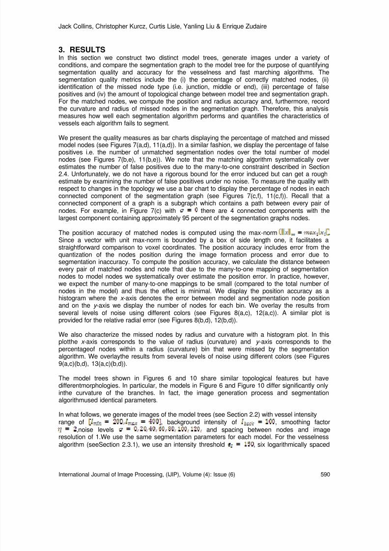
8/6/2019 International Journal of Image Processing (IJIP) Volume 4 Issue 6
http://slidepdf.com/reader/full/international-journal-of-image-processing-ijip-volume-4-issue-6 81/172
Jack Collins, Christopher Kurcz, Curtis Lisle, Yanling Liu & Enrique Zudaire
International Journal of Image Processing, (IJIP), Volume (4): Issue (6) 590
3. RESULTSIn this section we construct two distinct model trees, generate images under a variety ofconditions, and compare the segmentation graph to the model tree for the purpose of quantifyingsegmentation quality and accuracy for the vesselness and fast marching algorithms. Thesegmentation quality metrics include the (i) the percentage of correctly matched nodes, (ii)identification of the missed node type (i.e. junction, middle or end), (iii) percentage of false
positives and (iv) the amount of topological change between model tree and segmentation graph.For the matched nodes, we compute the position and radius accuracy and, furthermore, recordthe curvature and radius of missed nodes in the segmentation graph. Therefore, this analysismeasures how well each segmentation algorithm performs and quantifies the characteristics ofvessels each algorithm fails to segment.
We present the quality measures as bar charts displaying the percentage of matched and missedmodel nodes (see Figures 7(a,d), 11(a,d)). In a similar fashion, we display the percentage of falsepositives i.e. the number of unmatched segmentation nodes over the total number of modelnodes (see Figures 7(b,e), 11(b,e)). We note that the matching algorithm systematically overestimates the number of false positives due to the many-to-one constraint described in Section2.4. Unfortunately, we do not have a rigorous bound for the error induced but can get a roughestimate by examining the number of false positives under no noise. To measure the quality withrespect to changes in the topology we use a bar chart to display the percentage of nodes in eachconnected component of the segmentation graph (see Figures 7(c,f), 11(c,f)). Recall that aconnected component of a graph is a subgraph which contains a path between every pair ofnodes. For example, in Figure 7(c) with there are 4 connected components with thelargest component containing approximately 95 percent of the segmentation graphs nodes.
The position accuracy of matched nodes is computed using the max-norm .Since a vector with unit max-norm is bounded by a box of side length one, it facilitates astraightforward comparison to voxel coordinates. The position accuracy includes error from thequantization of the nodes position during the image formation process and error due tosegmentation inaccuracy. To compute the position accuracy, we calculate the distance betweenevery pair of matched nodes and note that due to the many-to-one mapping of segmentationnodes to model nodes we systematically over estimate the position error. In practice, however,we expect the number of many-to-one mappings to be small (compared to the total number ofnodes in the model) and thus the effect is minimal. We display the position accuracy as ahistogram where the x -axis denotes the error between model and segmentation node positionand on the y -axis we display the number of nodes for each bin. We overlay the results fromseveral levels of noise using different colors (see Figures 8(a,c), 12(a,c)). A similar plot isprovided for the relative radial error (see Figures 8(b,d), 12(b,d)).
We also characterize the missed nodes by radius and curvature with a histogram plot. In thisplotthe x -axis corresponds to the value of radius (curvature) and y -axis corresponds to thepercentageof nodes within a radius (curvature) bin that were missed by the segmentationalgorithm. We overlaythe results from several levels of noise using different colors (see Figures9(a,c)(b,d), 13(a,c)(b,d)).
The model trees shown in Figures 6 and 10 share similar topological features but have
differentmorphologies. In particular, the models in Figure 6 and Figure 10 differ significantly onlyinthe curvature of the branches. In fact, the image generation process and segmentationalgorithmused identical parameters.
In what follows, we generate images of the model trees (see Section 2.2) with vessel intensityrange of , background intensity of , smoothing factor
,noise levels and spacing between nodes and imageresolution of 1.We use the same segmentation parameters for each model. For the vesselnessalgorithm (seeSection 2.3.1), we use an intensity threshold , six logarithmically spaced
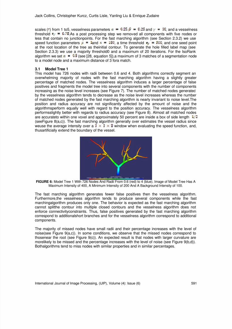
8/6/2019 International Journal of Image Processing (IJIP) Volume 4 Issue 6
http://slidepdf.com/reader/full/international-journal-of-image-processing-ijip-volume-4-issue-6 82/172
Jack Collins, Christopher Kurcz, Curtis Lisle, Yanling Liu & Enrique Zudaire
International Journal of Image Processing, (IJIP), Volume (4): Issue (6) 591
scales ( ) from 1 to5, vesselness parameters and , and a vesselnessthreshold .As a post processing step we removed all components with five nodes orless that contain no junctionpoints. For the fast marching algorithm (see Section 2.3.2) we usespeed function parameters and , a time threshold , and one seed pointat the root location of the tree as theinitial contour. To generate the hole filled label map (seeSection 2.3.3) we use a majority threshold0 and a maximum of 20 iterations. For the IsoRank
algorithm we set (see [28, equation 5]),a maximum of 3 matches of a segmentation nodeto a model node and a maximum distance of 3 fora match.
3.1 Model Tree 1This model has 726 nodes with radii between 0.6 and 4. Both algorithms correctly segment anoverwhelming majority of nodes with the fast marching algorithm having a slightly greaterpercentage of matched nodes. The vesselness algorithm induces a larger percentage of falsepositives and fragments the model tree into several components with the number of componentsincreasing as the noise level increases (see Figure 7). The number of matched nodes generatedby the vesselness algorithm tends to decrease as the noise level increases whereas the numberof matched nodes generated by the fast marching algorithm is nearly invariant to noise level.Theposition and radius accuracy are not significantly affected by the amount of noise and thealgorithmsperform equally well with regard to the position accuracy. The vesselness algorithmperformsslightly better with regards to radius accuracy (see Figure 8). Almost all matched nodesare accurateto within one voxel and approximately 50 percent are inside a box of side length(seeFigure 8(a,c)). The fast marching algorithm generally over estimates the vessel radius sinceweuse the average intensity over a window when evaluating the speed function, and,thusartificially extend the boundary of the vessel.
FIGURE 6: Model Tree 1 With 726 Nodes And Radii From 0.6 (red) to 4 (blue). Image of Model Tree Has AMaximum Intensity of 400, A Minimum Intensity of 200 And A Background Intensity of 100.
The fast marching algorithm generates fewer false positives then the vesselness algorithm.Furthermore,the vesselness algorithm tends to produce several components while the fastmarchingalgorithm produces only one. The behavior is expected as the fast marching algorithmcannot splitthe contour into multiple closed contours and the vesselness algorithm does notenforce connectivityconstraints. Thus, false positives generated by the fast marching algorithmcorrespond to additionalshort branches and for the vesselness algorithm correspond to additionalcomponents.
The majority of missed nodes have small radii and their percentage increases with the level ofnoise(see Figure 9(a,c)). In some conditions, we observe that the missed nodes correspond tothosenear the root (see Figure 9(c)). An expected result is that nodes with larger curvature aremorelikely to be missed and the percentage increases with the level of noise (see Figure 9(b,d)).Bothalgorithms tend to miss nodes with similar properties and in similar percentages.
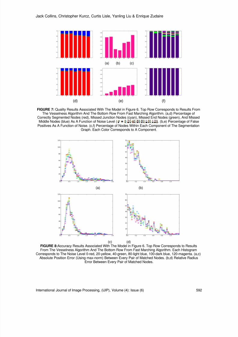
8/6/2019 International Journal of Image Processing (IJIP) Volume 4 Issue 6
http://slidepdf.com/reader/full/international-journal-of-image-processing-ijip-volume-4-issue-6 83/172
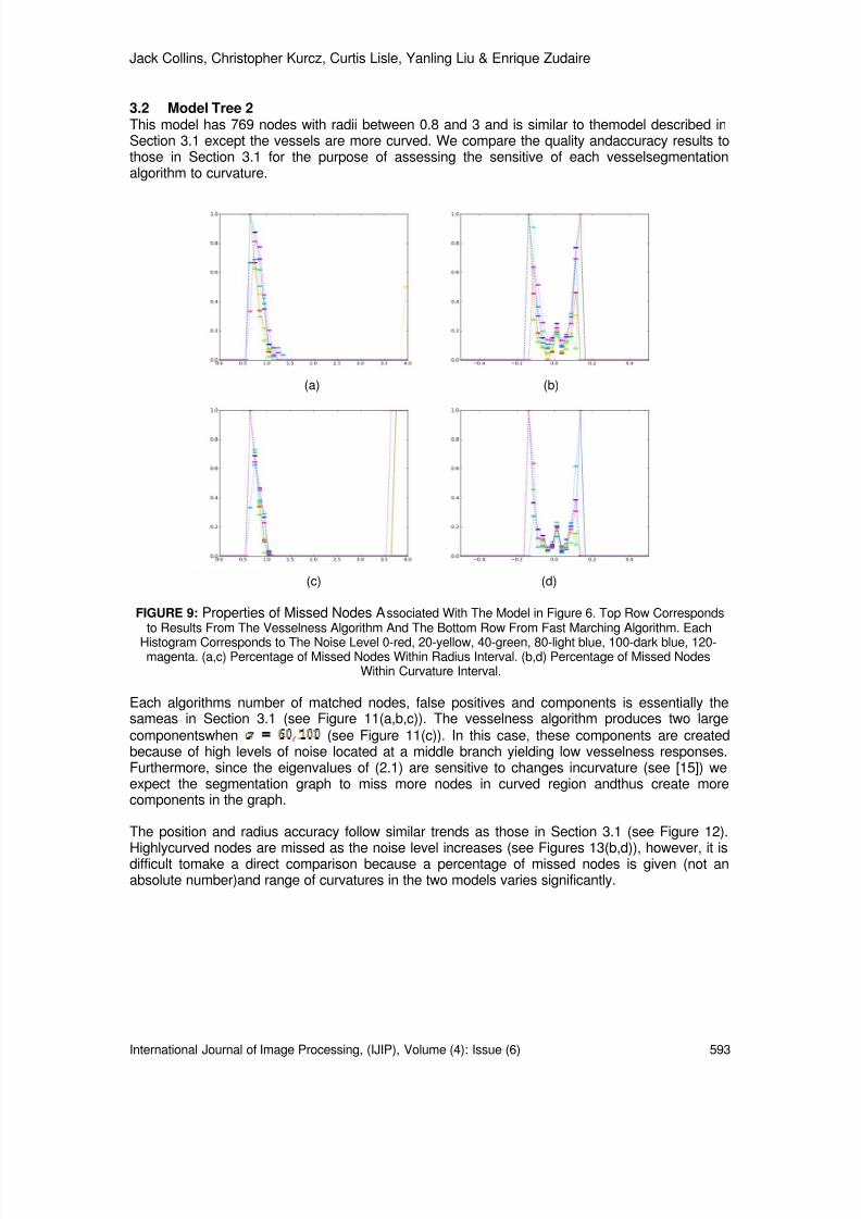
8/6/2019 International Journal of Image Processing (IJIP) Volume 4 Issue 6
http://slidepdf.com/reader/full/international-journal-of-image-processing-ijip-volume-4-issue-6 84/172
Jack Collins, Christopher Kurcz, Curtis Lisle, Yanling Liu & Enrique Zudaire
International Journal of Image Processing, (IJIP), Volume (4): Issue (6) 593
3.2 Model Tree 2This model has 769 nodes with radii between 0.8 and 3 and is similar to themodel described inSection 3.1 except the vessels are more curved. We compare the quality andaccuracy results tothose in Section 3.1 for the purpose of assessing the sensitive of each vesselsegmentationalgorithm to curvature.
(a) (b)
(c) (d)
FIGURE 9: Properties of Missed Nodes A ssociated With The Model in Figure 6. Top Row Correspondsto Results From The Vesselness Algorithm And The Bottom Row From Fast Marching Algorithm. Each
Histogram Corresponds to The Noise Level 0-red, 20-yellow, 40-green, 80-light blue, 100-dark blue, 120-magenta. (a,c) Percentage of Missed Nodes Within Radius Interval. (b,d) Percentage of Missed Nodes
Within Curvature Interval.
Each algorithms number of matched nodes, false positives and components is essentially thesameas in Section 3.1 (see Figure 11(a,b,c)). The vesselness algorithm produces two largecomponentswhen (see Figure 11(c)). In this case, these components are createdbecause of high levels of noise located at a middle branch yielding low vesselness responses.Furthermore, since the eigenvalues of (2.1) are sensitive to changes incurvature (see [15]) weexpect the segmentation graph to miss more nodes in curved region andthus create morecomponents in the graph.
The position and radius accuracy follow similar trends as those in Section 3.1 (see Figure 12).
Highlycurved nodes are missed as the noise level increases (see Figures 13(b,d)), however, it isdifficult tomake a direct comparison because a percentage of missed nodes is given (not anabsolute number)and range of curvatures in the two models varies significantly.
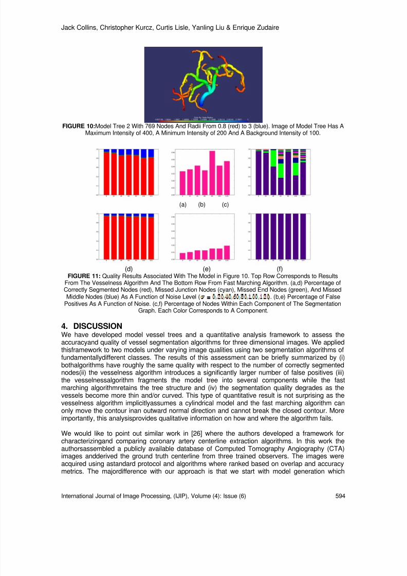
8/6/2019 International Journal of Image Processing (IJIP) Volume 4 Issue 6
http://slidepdf.com/reader/full/international-journal-of-image-processing-ijip-volume-4-issue-6 85/172
Jack Collins, Christopher Kurcz, Curtis Lisle, Yanling Liu & Enrique Zudaire
International Journal of Image Processing, (IJIP), Volume (4): Issue (6) 594
FIGURE 10: Model Tree 2 With 769 Nodes And Radii From 0.8 (red) to 3 (blue). Image of Model Tree Has AMaximum Intensity of 400, A Minimum Intensity of 200 And A Background Intensity of 100.
(a) (b) (c)
(d) (e) (f)FIGURE 11: Quality Results Associated With The Model in Figure 10. Top Row Corresponds to Results
From The Vesselness Algorithm And The Bottom Row From Fast Marching Algorithm. (a,d) Percentage ofCorrectly Segmented Nodes (red), Missed Junction Nodes (cyan), Missed End Nodes (green), And MissedMiddle Nodes (blue) As A Function of Noise Level ( ). (b,e) Percentage of False
Positives As A Function of Noise. (c,f) Percentage of Nodes Within Each Component of The SegmentationGraph. Each Color Corresponds to A Component.
4. DISCUSSIONWe have developed model vessel trees and a quantitative analysis framework to assess theaccuracyand quality of vessel segmentation algorithms for three dimensional images. We appliedthisframework to two models under varying image qualities using two segmentation algorithms offundamentallydifferent classes. The results of this assessment can be briefly summarized by (i)bothalgorithms have roughly the same quality with respect to the number of correctly segmentednodes(ii) the vesselness algorithm introduces a significantly larger number of false positives (iii)the vesselnessalgorithm fragments the model tree into several components while the fastmarching algorithmretains the tree structure and (iv) the segmentation quality degrades as thevessels become more thin and/or curved. This type of quantitative result is not surprising as the
vesselness algorithm implicitlyassumes a cylindrical model and the fast marching algorithm canonly move the contour inan outward normal direction and cannot break the closed contour. Moreimportantly, this analysisprovides qualitative information on how and where the algorithm fails.
We would like to point out similar work in [26] where the authors developed a framework forcharacterizingand comparing coronary artery centerline extraction algorithms. In this work theauthorsassembled a publicly available database of Computed Tomography Angiography (CTA)images andderived the ground truth centerline from three trained observers. The images wereacquired using astandard protocol and algorithms where ranked based on overlap and accuracymetrics. The majordifference with our approach is that we start with model generation which

8/6/2019 International Journal of Image Processing (IJIP) Volume 4 Issue 6
http://slidepdf.com/reader/full/international-journal-of-image-processing-ijip-volume-4-issue-6 86/172

8/6/2019 International Journal of Image Processing (IJIP) Volume 4 Issue 6
http://slidepdf.com/reader/full/international-journal-of-image-processing-ijip-volume-4-issue-6 87/172
Jack Collins, Christopher Kurcz, Curtis Lisle, Yanling Liu & Enrique Zudaire
International Journal of Image Processing, (IJIP), Volume (4): Issue (6) 596
We note that several improvements can be made to our framework and categorize them intomodelimprovements and analysis improvements. Depending on the application, a more detailedvascularmodel may be desired than the simple L-system approach employed here (see e.g. [14]).For example,a study in segmentation algorithms pertaining to angiogenesis could benefit from avesselmodel which more accurately reflects the vascular morphology in or near the tumorenvironment.Such methods typically use a system of reaction diffusion partial differentialequations (see e.g. [5])to model the growth of a vessel network. If the imaging modality is wellcharacterized, a better suited noise model (rather than additive Gaussian noise) can beimplemented. As pointed out in [33] aGaussian smoothed vessel cross section may beinsufficient. Since generating the image from themodel is explicit in our framework, changing thetype of convolution or averaging procedure to producea particular type of vessel cross sectionprofile is straightforward. Our model currently neglectsbackground objects and does not explicitlyincorporate vessel proximity to one another. A naturalextension to our assessment is multivariateanalysis of several properties. For example, we couldexamine if missed nodes have a correlationbetween radius, curvature or contrast.
The software developed in this paper was written using the following free and open sourcelibraries:Insight Toolkit [12] for image processing tasks, NetworkX [8] for the graphrepresentation, Matplotlib[11] for 2D plotting, and Mayavi [22] for 3D plotting.
(a) (b)
(c) (d)
FIGURE 13: Properties of Missed Nodes A ssociated With The Model in Figure 10. Top Row
Corresponds to Results From The Vesselness Algorithm And The Bottom Row From Fast MarchingAlgorithm. Each Histogram Corresponds to The Noise Level 0-red, 20-yellow, 40-green, 80-light blue, 100-dark blue, 120-magenta. (a,c) Percentage of Missed Nodes Within Radius Interval. (b,d) Percentage of
Missed Nodes Within Curvature Interval.
ACKNOWLEDGMENTThis project has been funded in whole or in part with federal funds from the National CancerInstitute, National Institutes of Health, under Contract No. HHSN261200800001E. The content ofthis publication does not necessarily reflect the views or policies of the Department of Health and

8/6/2019 International Journal of Image Processing (IJIP) Volume 4 Issue 6
http://slidepdf.com/reader/full/international-journal-of-image-processing-ijip-volume-4-issue-6 88/172
Jack Collins, Christopher Kurcz, Curtis Lisle, Yanling Liu & Enrique Zudaire
International Journal of Image Processing, (IJIP), Volume (4): Issue (6) 597
Human Services, nor does mention of trade names, commercial products, or organizations implyendorsement by the U.S. Government.
5. REFERENCES
1. L. Antiga, M. Piccinelli, L. Botti, B. Ene-Iordache, A. Remuzzi, and D. A. Steinman. “An
image-based modeling framework for patient-specific computational hemodynamics” . Medical& Biological Engineering & Computing, 46:1097-1112, November 2008.
2. E. Bullitt, M. Ewend, J. Vredenburgh, A. Friedman, W. Lin, K. Wilber, D. Zeng, S. R. Aylward,and D. Reardon. “Computerized assessment of vessel morphological changes during treatment of glioblastoma multiforme: report ofa case imaged serially by MRA over four years” . Neuroimage, 47(Supplement 2):T143-151, August 2009.
3. F. Cassot, F. Lauwers, C. Fouard, S. Prohaska, and V. Lauwers-Cances. “A novel three- dimensional computer-assistedmethod for a quantitative study of microvascular networks of the human cerebral cortex” . Microcirculation,13:1-18, January 2006.
4. R. M. Cesar, Jr., E. Bengoetxea, I. Bloch, and P. Larrañaga. “Inexact graph matching for
modelbasedrecognition: Evaluation and comparison of optimization algorithms” . PatternRecognition, 38(11):2099-2113,2005.
5. M. A. Chaplain, S. R. McDougall, and A. R. Anderson. “Mathematical modeling of tumor- induced angiogenesis” .Annual Review of Biomedical Engineering, 8:233-257, 2006.
6. D. Conte, P. Foggia, C. Sansone, and M. Vento. “Thirty years of graph matching in patternrecognition” . International Journal of Pattern Recognition and Artificial Intelligence,18(3):265-298.
7. A. F. Frangi, R. F. Frangi, W. J. Niessen, K. L. Vincken, and M. A. Viergever. “Multiscale vesselenhancement filtering” . Medical Image Computing and Computer-AssistedInterventation, 1998.
8. A. A. Hagberg, D. A. Schult, and P. J. Swart. “Exploring network structure, dynamics, and function usingNetworkX” . In Proceedings of the 7th Python in Science Conference,Pasadena, CA, USA, August 2008.
9. H. Homann. “Implementation of a 3D thinning algorithm” . Insight Journal, 2007.http://hdl.handle.net/1926/1292.
10. H. Honda. “Description of the form of trees by the parameters of the tree-like body: Effects of the branching angleand the branch length on the shape of the tree-like body” . Journal ofTheoretical Biology, 31(2):331-338, 1971.
11. J. D. Hunter. “Matplotlib: A 2d graphics environment” . Computing in Science andEngineering, 9(3):90-95, 2007.
12. L. Ibanez, W. Schroeder, L. Ng, and J. Cates. “The ITK Software Guide” . Kitware, Inc., 2005.
13. C. Kirbas and F. Quek. “A review of vessel extraction techniques and algorithms” . ACMComputing Surveys,36(2):81-121, 2004.
14. G. Kokai, Z. Toth, and R. Vanyi. “Modelling blood vessels of the eye with parametric L- systems usingevolutionary algorithms” . In Proceedings of the Joint European Conference

8/6/2019 International Journal of Image Processing (IJIP) Volume 4 Issue 6
http://slidepdf.com/reader/full/international-journal-of-image-processing-ijip-volume-4-issue-6 89/172
Jack Collins, Christopher Kurcz, Curtis Lisle, Yanling Liu & Enrique Zudaire
International Journal of Image Processing, (IJIP), Volume (4): Issue (6) 598
onArtificial Intelligence in Medicine and Medical Decision Making, Aalborg, Denmark, June1999.
15. K. Krissian, G. Malandain, N. Ayache, R. Vaillant, and Y. Trousset. “Model-based detection oftubular structures in 3d images” . Computer Vision and Image Understanding, 80(2):130-171, 2000.
16. A. N. Langville and C. D. Meyer. “Google’s PageRank and Beyond: The Science of Search Engine Rankings” .Princeton University Press, Princeton, NJ, USA, 2006.
17. A. Lindenmayer. “ Mathematical models for cellular interactions in development i. filaments with one-sided inputs” .Journal of Theoretical Biology, 18(3):280-299, 1968.
18. A. Lindenmayer. “Mathematical models for cellular interactions in development ii. simple and branching filamentswith two-sided inputs” . Journal of Theoretical Biology, 18(3):300-315,1968.
19. S. Luo and Y. Zhong. “Extraction of brain vessels from magnetic resonance angiographic images: concise literaturereview, challenges, and proposals” . In Proceedings of IEEEEngineering in Medicine and Biology Society, 2:1422-1425, 2005.
20. F. Nekka, S. Kyriacos, C. Kerrigan, and L. Cartilier. “A model of growing vascular structures” .Bulletin of Mathematical Biology, 58:409-424, May 1996.
21. W. Palubicki, K. Horel, S. Longay, A. Runions, B. Lane, R. M ĕ ch, and P. Prusinkiewicz. “Self- organizing tree models for image synthesis” . In Proceedings of ACM SIGGRAPH 2009, NewYork, NY, USA, 2009.
22. P. Ramachandran. “MayaVi: A free tool for CFD data visualization” . 4th Annual CFDSymposium, AeronauticalSociety of India, 2001.
23. X. Qian, M. P. Brennan, D. P. Dione, W. L. Dobrucki, M. P. Jackowski, C. K. Breuer, A. J.Sinusas, and X. Papademetris. “A non-parametric vessel detection method for complex
vascular structures” . Medical Image Analysis, 13(1):49–61, February 2009.
24. G. Rozenberg and A. Salomaa, editors. “Lindenmayer Systems: Impacts on Theoretical Computer Science,Computer Graphics, and Developmental Biology” . Springer-Verlag NewYork, Inc., Secaucus, NJ, USA, 2001.
25. Y. Sato, S. Nakajima, N. Shiraga, H. Atsumi, S. Yoshida, T. Koller, G. Gerig, and R. Kikinis.“Three-dimensionalmulti-scale line filter for segmentation and visualization of curvilinear structures in medical images” . Medical Image Analysis, 2(2):143-168, 1998.
26. M. Schaap, C. T. Metz, T. van Walsum, A. G. van der Giessen, A. C. Weustink, N. R. Mollet,C. Bauer, H. Bogunovi,C. Castro, X. Deng, E. Dikici, T. O’Donnell, M. Frenay, O. Friman, M.Hernandez Hoyos, P. H. Kitslaar, K. Krissian,C. Kuhnel, M. A. Luengo-Oroz, M. Orkisz, O.
Smedby, M. Styner, A. Szymczak, H. Tek, C. Wang, S. K. Warfield,S. Zambal, Y. Zhang, G.P. Krestin, and W. J. Niessen. “Standardized evaluation methodology and reference databasefor evaluating coronary artery centerline extraction algorithms” . Medical ImageAnalysis, 13(5):701-714, October 2009.
27. J. A. Sethian. “Level Set Methods and Fast Marching Methods” . Cambridge University Press,1999.

8/6/2019 International Journal of Image Processing (IJIP) Volume 4 Issue 6
http://slidepdf.com/reader/full/international-journal-of-image-processing-ijip-volume-4-issue-6 90/172
Jack Collins, Christopher Kurcz, Curtis Lisle, Yanling Liu & Enrique Zudaire
International Journal of Image Processing, (IJIP), Volume (4): Issue (6) 599
28. R. Singh, J. Xu, and B. Berger. “Global alignment of multiple protein interaction networks with application to functionalorthology detection” . In Proceedings of the National Academy ofSciences of the United States of America. 105(35):12763-12768, September 2008.
29. M. Sofka and C. V. Stewart. “Retinal vessel centerline extraction using multiscale matched filters, confidence andedge measures” . IEEE Transactions on Medical Imaging, 25(12):1531– 1546, Dec 2006.
30. S. Thoreson. “An efficient solution to inexact graph matching with application to computer vision” . PhD thesis,Norwegian University of Science and Technology, 2007.
31. N.J. Tustison, M.Siqueira, and J.C.Gee. “N-D Linear Time Exact Signed Euclidean Distance Transform” . InsightJournal, 2006. http://hdl.handle.net/1926/171.
32. J. R. Ullmann. “An algorithm for subgraph isomorphism” . Journal of ACM, 23(1):31-42,January 1976.
33. S. Worz and K. Rohr. “Segmentation and quantification of human vessels using a 3-D cylindrical intensity model” .IEEE Transactionson Image Processing, 16(8):1994-2004, Aug2007.
34. P. J. Yim, P. L. Choyke, and R. M. Summers. “Gray-scale skeletonization of small vessels in magnetic resonanceangiography” . IEEE Transactions on Medical Imaging, 19(6):568–576,June 2000.

8/6/2019 International Journal of Image Processing (IJIP) Volume 4 Issue 6
http://slidepdf.com/reader/full/international-journal-of-image-processing-ijip-volume-4-issue-6 91/172
Ojo, John Adedapo & Adeniran, Solomon A.
International Journal of Image Processing (IJIP), Volume (4): Issue (6) 600
Colour Face Image Database for Skin Segmentation, FaceDetection, Recognition and Tracking of Black Faces Under Real-
Life Situations
OJO, John Adedapo [email protected] of Electronic & Electrical Engineering,Ladoke Akintola University of Technology (LAUTECH),Ogbomoso, P.M.B. 4000, Nigeria.
Adeniran, Solomon A [email protected] of Electronic & Electrical Engineering,Obafemi Awolowo University (OAU),Ile Ife, Nigeria.
Abstract
This paper presents a new face database containing only black face images. It isdesigned to be used for benchmarking algorithms developed for skinsegmentation, face detection and recognition under real life situations. Thedatabase contains coloured images of black faces in JPEG formats taken over aperiod of two years (2007-2009). It contains three subfolders, where the imageshave been grouped for face detection, face recognition and face trackingpurposes. There are over 100 images for face detection containing more than150 face images and 600 images of ten per 60 individuals for face recognitionand 10s video sequences of ten black faces. An interactive Graphic UserInterface (GUI) was developed in Matlab® (7.4.1a version) for the face databaseproviding basic information about the images as well as creating an interactiveand easy to use environment.
Keywords: Skin Segmentation; Face Detection; Face Recognition; Face Tracking
1. INTRODUCTION
To benchmark face detection or face recognition algorithms, the use of standard datasets isrecommended as this would allow researchers to their compare results. Since there are varietiesof large databases, the choice of an appropriate one to select is based on the problem(s)intended to be solved. The common face databases are the AT&T face database [1] and the MITdatabase ( http://www.ai.mit.edu/projects/cbcl ). Others that have been mentioned and usedare the MATRANORTEL database [2], AR face database [3], and FERET database [4,5].
Image is formed in the eye and in the camera by the amount of illumination reflected by an object.This explains why capturing, detecting and recognition of faces of different skin colour is of highimportance. Recent studies have shown that pigmentation (i.e. surface reflectance properties,including albedo, hue, specularity, translucency, and spatial variation in these properties) cuesare equally as important as shape information for face recognition [6].
In the face recognition homepage ( http://www.face_rec.org/databases/ ), about 35 facedatabases were reported to exist as at July 2008. In the handbook of face recognition, 20 facedatabases for face recognition, 2 for face detection, 5 for non-face and sub-face datasets and 3

8/6/2019 International Journal of Image Processing (IJIP) Volume 4 Issue 6
http://slidepdf.com/reader/full/international-journal-of-image-processing-ijip-volume-4-issue-6 92/172
Ojo, John Adedapo & Adeniran, Solomon A.
International Journal of Image Processing (IJIP), Volume (4): Issue (6) 601
for facial expression analysis were reviewed [7]. The summary of some of the face databases ispresented in Table 1. They include FERET database [4,5], AT&T (formerly ORL) [1], AR (Purdue)database [3], CMU PIE database [8], Indian face database [9], Chinese Academy of Sciences(CAS) database [10] and VT-AAST image database [11]. In these databases, face images werecaptured under controlled conditions which are far from what is obtainable in the real life. Forexample, the cameras used for surveillance have much more lower resolutions compared to theones reported to have been used in capturing the images in these databases. In addition,surveillance cameras do not have the capacity or added function of providing flash when animage is to be captured, whereas most of the images in the earlier databases used either flashesor were taken under standard lighting conditions.
We venture to bridge the gap in the existing databases especially for the detection andrecognition of Black faces. Black surfaces reflect a small fraction of the light rays incident onthem. Therefore, under very poor illumination conditions, very little information is made availablefor processing, detection or recognition. Recent report have countered the notion that color isunimportant for human face recognition and suggested instead that when shape cues in imagesare compromised (e.g. by reductions in resolution), the brain relies on color cues to pinpointidentity [12,13].
This paper presents a new face database which contains only black face images of different skintones, middle aged and both male and female gender. It is designed to be used for benchmarkingalgorithms developed for face detection, recognition and tracking under real-life conditions.Section 2 gives a description of the database, how it was populated and the results of skinsegmentation performed on some of the images in the database and section 3 gives theconclusion.
2. BLACK FACE DATABASE (BFDB)
The Black-face Database comprises of two parts, Part A was taken to serve as a pilot to thesecond Part B and for use in the early part of a research work [14], the Part B is being developedto increase the robustness of the database for benchmarking face detection, recognition and facetracking algorithms, with its own peculiar advantage. The Part A of the database is fully reportedin this paper, while work is in progress on Part B of the database. Each Part contains three sub-folders; containing images for face detection, face recognition and video sequence of faces forface tracking.
The face detection folder ‘Detect’ contains 10 uncompressed pictures containing at least 45faces. The images were captured at different dates and periods of the day and contain imageswith different pose, orientation, gender, background and illumination. A summary of the images inthe ‘Detect’ subfolder is shown in Table 2. The face recognition folder contains 123 images of 20persons taken under different conditions with varying facial expressions, details are shown inTable 3. The pictures were taken between August 2008 and April, 2009. The pictures were takenwith Hp 7.3 Mega-pixels camera and they are in JPEG formats. The pictures were later croppedand compressed to 448×336 pixels. Compressing the images did not necessarily affect skindetection but the time of execution was faster than when the images were not compressed [14].
The database contains twenty folders each containing at least five upright and frontal pictures ofeach subject (person). Each folder comprises of frontal images of each subject taken without theuse of flashes. There are three variations under the illumination which are; controlled lighting,labelled as ‘bright’; outdoor but dull illumination labelled as ‘poor’; and under dark illuminationlabelled as ‘dark’. The variations in facial expressions were ‘smile’, ‘frown’ and ‘blink’. Shots ofsubject with their heads slightly rotated to the right and to the left were also taken to achievevariations in pose and were labelled ‘right’ and ‘left’ respectively. At least one of the subjects hada scarf on and at least another one was in glasses. Examples of images of two subjects (persons)are shown in Figure 1.
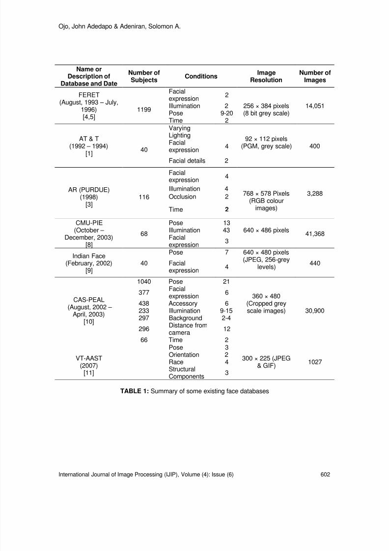
8/6/2019 International Journal of Image Processing (IJIP) Volume 4 Issue 6
http://slidepdf.com/reader/full/international-journal-of-image-processing-ijip-volume-4-issue-6 93/172
Ojo, John Adedapo & Adeniran, Solomon A.
International Journal of Image Processing (IJIP), Volume (4): Issue (6) 602
TABLE 1: Summary of some existing face databases
Name orDescription of
Database and Date
Number ofSubjects Conditions Image
ResolutionNumber of
Images
FERET(August, 1993 – July,1996)[4,5]
1199
Facialexpression 2
256 × 384 pixels(8 bit grey scale)
14,051Illumination 2Pose 9-20Time 2
AT & T(1992 – 1994)
[1] 40
VaryingLighting 92 × 112 pixels
(PGM, grey scale) 400Facialexpression 4
Facial details 2
AR (PURDUE)(1998)[3]
116
Facialexpression 4
768 × 578 Pixels(RGB colour
images)
3,288Illumination 4Occlusion 2
Time 2
CMU-PIE(October –
December, 2003)[8]
68
Pose 13640 × 486 pixels 41,368Illumination 43
Facialexpression 3
Indian Face(February, 2002)
[9]40
Pose 7 640 × 480 pixels(JPEG, 256-grey
levels) 440Facialexpression 4
CAS-PEAL(August, 2002 –
April, 2003)[10]
1040 Pose 21
360 × 480(Cropped greyscale images) 30,900
377 Facialexpression 6
438 Accessory 6233 Illumination 9-15297 Background 2-4
296 Distance fromcamera 12
66 Time 2
VT-AAST(2007)
[11]
Pose 3
300 × 225 (JPEG& GIF) 1027
Orientation 2Race 4StructuralComponents 3

8/6/2019 International Journal of Image Processing (IJIP) Volume 4 Issue 6
http://slidepdf.com/reader/full/international-journal-of-image-processing-ijip-volume-4-issue-6 94/172
Ojo, John Adedapo & Adeniran, Solomon A.
International Journal of Image Processing (IJIP), Volume (4): Issue (6) 603
FIGURE 1: Examples of images in the face recognition database
Part B of the database contains two folders, ‘detect’ and ‘recognition’ folders. The ‘detect’ foldercontains two folders, one contains images captured under good illumination (‘Light’) while theother contains images captured under poor illumination (“Dark’). The light folder has 50 imageswhich contain at least 72 human faces of varying poses and illumination captured under goodlighting condition. Few images were adopted from the internet one or two existing databases. Thedark folder has 50 images which contain at least 68 human faces of varying poses andorientations taken under poor illumination. A summary is given in Table 3 and examples ofimages captured under good and poor illuminations are shown in Figures 2a and 2b respectively.
(a) Images taken under good illumination
(a) Images taken under poor illuminationFIGURE 2: Examples of images in the face detection database
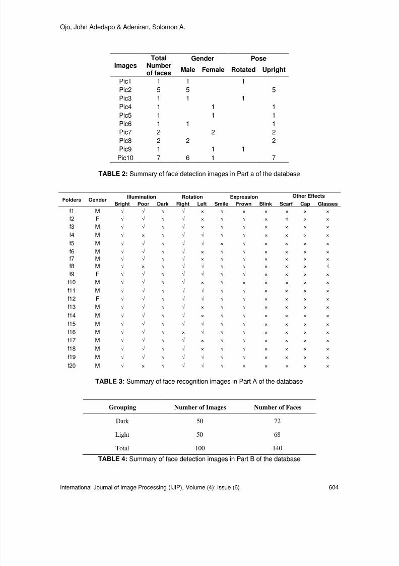
8/6/2019 International Journal of Image Processing (IJIP) Volume 4 Issue 6
http://slidepdf.com/reader/full/international-journal-of-image-processing-ijip-volume-4-issue-6 95/172
Ojo, John Adedapo & Adeniran, Solomon A.
International Journal of Image Processing (IJIP), Volume (4): Issue (6) 604
ImagesTotal
Numberof faces
Gender Pose
Male Female Rotated Upright
Pic1 1 1 1Pic2 5 5 5
Pic3 1 1 1Pic4 1 1 1Pic5 1 1 1Pic6 1 1 1Pic7 2 2 2Pic8 2 2 2Pic9 1 1 1
Pic10 7 6 1 7
TABLE 2: Summary of face detection images in Part a of the database
Folders Gender Illumination Rotation Expression Other EffectsBright Poor Dark Right Left Smile Frown Blink Scarf Cap Glasses
f1 M √ √ √ √ × √ × × × × ×f2 F √ √ √ √ × √ √ × √ × ×f3 M √ √ √ √ × √ √ × × × ×f4 M √ × √ √ √ √ √ × × × ×f5 M √ √ √ √ √ × √ × × × ×f6 M √ √ √ √ × √ √ × × × ×f7 M √ √ √ √ × √ √ × × × ×f8 M √ × √ √ √ √ √ × × × √ f9 F √ √ √ √ √ √ √ × × × ×
f10 M √ √ √ √ × √ × × × × ×f11 M √ √ √ √ √ √ √ × × × ×
f12 F √ √ √ √ √ √ √ × × × ×f13 M √ √ √ √ × √ √ × × × ×f14 M √ √ √ √ × √ √ × × × ×f15 M √ √ √ √ √ √ √ × × × ×f16 M √ √ √ × √ √ √ × × × ×f17 M √ √ √ √ × √ √ × × × ×f18 M √ √ √ √ × √ √ × × × ×f19 M √ √ √ √ √ √ √ × × × ×f20 M √ × √ √ √ √ × × × × ×
TABLE 3: Summary of face recognition images in Part A of the database
Grouping Number of Images Number of Faces
Dark 50 72
Light 50 68
Total 100 140
TABLE 4: Summary of face detection images in Part B of the database

8/6/2019 International Journal of Image Processing (IJIP) Volume 4 Issue 6
http://slidepdf.com/reader/full/international-journal-of-image-processing-ijip-volume-4-issue-6 96/172
Ojo, John Adedapo & Adeniran, Solomon A.
International Journal of Image Processing (IJIP), Volume (4): Issue (6) 605
An interactive Graphic User Interface (GUI) was developed in Matlab TM 7.4.1a version for the facedatabase to enable an easier use. This is also an improvement over other face databases. Boththe database would be copied at a known location on the user’s computer and the Matlab filewould be copied into the Matlab directory. The user then only needs to type the default filename“face_database in the Matlab command prompt. The interactive GUI would appear and theneeded image can be selected. The user would type in the address or location of the databaseinto the query, then select the exact image to be used. The image can then be saved and usedfor either face detection, training or testing a face recognition algorithm. The default filename forthe face detection GUI is Database_detect. The outlooks of the GUIs are in Figures 3 and 4. Thedatabase as well as the Matlab® codes can be obtained by contacting the authors.
FIGURE 3: Matlab GUI for Face Detection Database
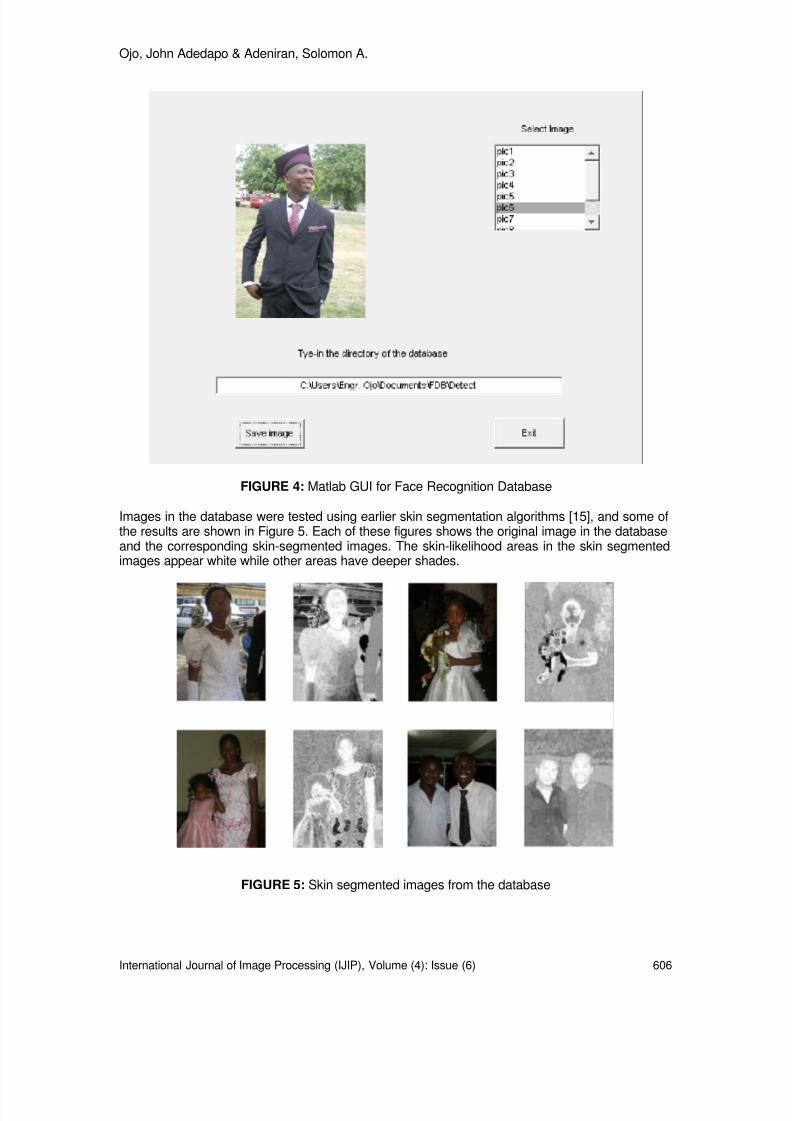
8/6/2019 International Journal of Image Processing (IJIP) Volume 4 Issue 6
http://slidepdf.com/reader/full/international-journal-of-image-processing-ijip-volume-4-issue-6 97/172
Ojo, John Adedapo & Adeniran, Solomon A.
International Journal of Image Processing (IJIP), Volume (4): Issue (6) 606
FIGURE 4: Matlab GUI for Face Recognition Database
Images in the database were tested using earlier skin segmentation algorithms [15], and some ofthe results are shown in Figure 5. Each of these figures shows the original image in the databaseand the corresponding skin-segmented images. The skin-likelihood areas in the skin segmentedimages appear white while other areas have deeper shades.
FIGURE 5: Skin segmented images from the database

8/6/2019 International Journal of Image Processing (IJIP) Volume 4 Issue 6
http://slidepdf.com/reader/full/international-journal-of-image-processing-ijip-volume-4-issue-6 98/172
Ojo, John Adedapo & Adeniran, Solomon A.
International Journal of Image Processing (IJIP), Volume (4): Issue (6) 607
FIGURE 6: Selected images from the database showing detected faces.
Images in the face detection subfolder were tested for presence of faces using a novel facedetection algorithm [16]. Some of ths results are shown in Figure 6. Detection rates of 83.8% and76.4% were achieved for faces captured under good and poor illumination respectively. Thesame images were tested with earlier algorithms which have been reported to have goodperformances [17,18], details shown in Table 5. It is observed that although the earlier algorithmsperformed excellently well when benchmarked on some face detection databases, it was not sowith the new database (BFDB). As a result, the new database with its unique feature of largevariations under real life situations is expected create new frontiers for researches in facedetection and recognition.
Detection Method
Detection Rates
Good
illumination
Poor
illumination
Hybrid Model [16] 83.8% 76.4%
Viola & Jones [17] 35.29% 31.94%
Pai et al [18] 66.18% 56.9%
TABLE 5: Detection rates for images taken under good Illumination
3. CONSLUSIONThis paper has discussed a new face database developed to solve some challenges poised inusing appropriate images to benchmark algorithms developed for skin-segmentation, facedetection, recognition and face tracking, especially for Black faces. It contains images takenunder large variations under real life situations and it gave good results in the study of skin-segmentation.
8/6/2019 International Journal of Image Processing (IJIP) Volume 4 Issue 6
http://slidepdf.com/reader/full/international-journal-of-image-processing-ijip-volume-4-issue-6 99/172
Ojo, John Adedapo & Adeniran, Solomon A.
International Journal of Image Processing (IJIP), Volume (4): Issue (6) 608
4. REFERENCES
1. F. Samaria and A. Harter (1994), Parameterization of a Stochastic Model for Human faceIdentification. 2nd IEEE Workshop on Applications of Computer Vision, Saratosa FL.December, 1994, pp 138-142 Available at: http://www.uk.research.att.co/faceddatabased.html [Accessed 20 October 2007]
2. A. Tefas, Y. Menguy, O. Kotropoulos, G. Richard, I. Pitas and P.C. Lockwood.“Compensating for Variable Recording Conditions in Frontal Face Authentication Algorithms”. IEEE International Conference on Acoustics, Speech and Signal Processing, (6)3561 – 3564,1999
3. A.R. Martine and R. Benavente (1998), “The AR Face Database,” CVC Technical Report 24,Computer Vision Centre (CVC). Technical Report, Barcelona. Available at:http://rvll.ecn.purdue.edu/~alex/alex-face-Db.html [Accessed 12 July 2009]
4. P.J. Phillips, H. Wechsler and P. Rauss “The FERET Database and Evaluation Procedure for face Recognition Algorithms”. Image and Vision Computing, 16(5):295-306, 1998
5. P.J. Phillips. H. Moon, S.A. Rizvi and P.J. Rauss. “The FERET Evaluation Methodology for Face-Recognition Algorithms” . IEEE Transaction on Pattern Analysis and MachineIntelligence. 22(10):1090-1104, 2000
6. S.E. Umbaugh. “Computer Vision and Image Processing: A Practical Approach Using CVIP tools”. Prentice-Hall International, Inc., N.J. USA, pp. 12-24 (1998)
7. R. Gross. “Face Database”. In S.Z. Li and A.K. Jain (Eds.) Handbook of Face Recognition.
Springer-Verlag., pp. 301-328 (2005)8. T. Sim, S. Baker and M. Bsat. “The CMU Pose, Illumination and Expression Database”. IEEE
Transactions on Pattern Analysis and Machine Intelligence, 25(12):1615-1618, 2003.
9. V. Jain and A. Mukherjee (2002), The Indian Face Database [online], Available at: http://vis-www.is.umass.edu/~vidit/IndianFaceDatabase2002 [Accessed 7 November 2008]
10. W. Gao, B. Cao, S. Shans, D. Zhou, X. Zhang and D. Zhao (2004) CASP-PEAL Large ScaleChinese Face Database and Evaluation Protocols Technical Report. JDL-TR-04FR-001[online], Joint research Development laboratory. Available at:http://www.jdl.ac.cn/peal/index.html [Accessed 10 June 2008]
11. A.S. Abdallah, M.A. El-Nasr and A.C. Abbott. “A New Colour Image Database for Benchmarking of Automatic Face Detection and Human Skin Segmentation Techniques”. Proceedings of World Academy of Science, Engineering and Technology, 20:353-357, 2007
12. P. Sinha, B. Balas, O. Yuri, and R. Russell. “Face Recognition by Humans: Nineteen Results All Computer Vision Researchers Should Know About”. Proceedings of the IEEE,94(11):1948-1962, November 2006

8/6/2019 International Journal of Image Processing (IJIP) Volume 4 Issue 6
http://slidepdf.com/reader/full/international-journal-of-image-processing-ijip-volume-4-issue-6 100/172
Ojo, John Adedapo & Adeniran, Solomon A.
International Journal of Image Processing (IJIP), Volume (4): Issue (6) 609
13. A. Yip and P. Sinha. “Role of color in face recognition”. Perception , 31: 995–1003, 2002.
14. J.A. Ojo, S.A., Adeniran, and T.I. Raji. “Developing Face Database for Detection and Recognition of Black Faces under Real-Life Situations”. In Book of Abstracts, 1 st Postgraduate Research Symposium, Faculty of Engineering & Technology, LAUTECH,Ogbomoso, Nigeria, 10 -11th March, 2010
15. J. Cai and A. Goshtasby (1999), “Detecting Human Faces in Colour-Images”. Image andVision Computing, (18):63-75, 1999
16. J.A. Ojo, S.A., Adeniran and T.I. Raji (2010). “Robust Face Detection Algorithm.” Paperaccepted for publication in Global Journal of Engineering & Technology, Vol 3, No 3.
17. P. Viola and M. Jones (2004). “Robust Real-Time Face Detection.” International Journal ofComputer Vision, 57(2), 137-154.
18. Y.-T, Pai, S.-J. Raun, M.-C., Shie and Y.-C. Liu (2006). “A Simple and Accurate Colour Face Detection Algorithm in Complex Background.” IEEE International Conference on Multimedia
and Expo. Pp 1545-1548.

8/6/2019 International Journal of Image Processing (IJIP) Volume 4 Issue 6
http://slidepdf.com/reader/full/international-journal-of-image-processing-ijip-volume-4-issue-6 101/172
Jigisha N. Patel, Suprava Patnaik & Vaibhavi P. Lineswala
International Journal of Image Processing (IJIP), Volume (4): Issue (6) 610
Rate Distortion Performance for Joint Source Channel Codingof JPEG Image Over AWGN Channel
Prof. Jigisha N. Patel [email protected] Assistant Professor, ECED,s v national institute of tech.surat,395007,india
Dr Suprava Patnaik [email protected] Professor, ECED,s v national institute of tech.surat,395007,india
Ms.Vaibhavi P. Lineswala [email protected] Student, ECED,s v national institute of tech.
surat,395007,india
Abstract
This paper presents the rate distortion behavior of Joint Source Channel Coding(JSCC) scheme for still image transmission. The focus is on DCT based sourcecoding JPEG, Rate Compatible Punctured Convolution Codes (RCPC) fortransmission over Additive White Gaussian Noise (AWGN) channel under theconstraint of fixed transmission bandwidth. Information transmission has atradeoff between compression ratio and received quality of image. Thecompressed stream is more susceptible to channel errors, thus error control
coding techniques are used along with images to minimize the effect of channelerrors. But there is a clear tradeoff between channel coding redundancies versussource quality with constant channel bit rate. This paper proposes JSCC schemebased on Unequal Error Protection (UEP) for robust image transmission. Withthe conventional error control coding schemes that uses Equal Error Protection(EEP), all the information bits are equally protected. The use of the UEPschemes provides a varying amount of error protection according to theimportance of the data. The received image quality can be improved using UEPcompared to Equal Error Protection (EEP).
Keywords: JPEG, Convolution Code, Puncturing, JSCC, UEP, EEP
1. INTRODUCTIONWith rapid growth of data communication infrastructure, there has been an increasing demand formultimedia communication services involving image communication over wireless channels. Twocommon problems encountered in multimedia communication services are large bandwidthrequirement and noisy transmission channels. Communication channels have limited resourcessuch as bandwidth and power, and multimedia sources usually contain significant amount of
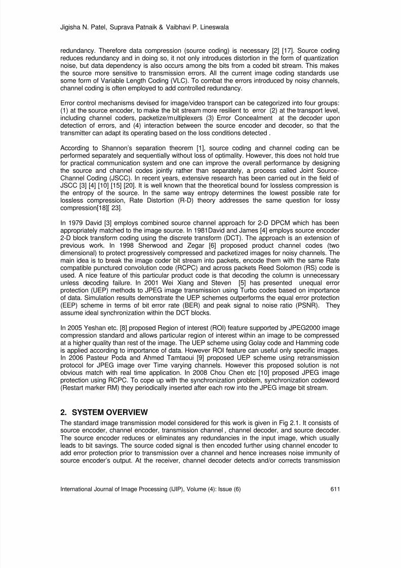
8/6/2019 International Journal of Image Processing (IJIP) Volume 4 Issue 6
http://slidepdf.com/reader/full/international-journal-of-image-processing-ijip-volume-4-issue-6 102/172
Jigisha N. Patel, Suprava Patnaik & Vaibhavi P. Lineswala
International Journal of Image Processing (IJIP), Volume (4): Issue (6) 611
redundancy. Therefore data compression (source coding) is necessary [2] [17]. Source codingreduces redundancy and in doing so, it not only introduces distortion in the form of quantizationnoise, but data dependency is also occurs among the bits from a coded bit stream. This makesthe source more sensitive to transmission errors. All the current image coding standards usesome form of Variable Length Coding (VLC). To combat the errors introduced by noisy channels,channel coding is often employed to add controlled redundancy.
Error control mechanisms devised for image/video transport can be categorized into four groups:(1) at the source encoder, to make the bit stream more resilient to error (2) at the transport level,including channel coders, packetize/multiplexers (3) Error Concealment at the decoder upondetection of errors, and (4) interaction between the source encoder and decoder, so that thetransmitter can adapt its operating based on the loss conditions detected .
According to Shannon’s separation theorem [1], source coding and channel coding can beperformed separately and sequentially without loss of optimality. However, this does not hold truefor practical communication system and one can improve the overall performance by designingthe source and channel codes jointly rather than separately, a process called Joint Source-Channel Coding (JSCC). In recent years, extensive research has been carried out in the field ofJSCC [3] [4] [10] [15] [20]. It is well known that the theoretical bound for lossless compression isthe entropy of the source. In the same way entropy determines the lowest possible rate forlossless compression, Rate Distortion (R-D) theory addresses the same question for lossycompression[18][ 23].
In 1979 David [3] employs combined source channel approach for 2-D DPCM which has beenappropriately matched to the image source. In 1981David and James [4] employs source encoder2-D block transform coding using the discrete transform (DCT). The approach is an extension ofprevious work. In 1998 Sherwood and Zegar [6] proposed product channel codes (twodimensional) to protect progressively compressed and packetized images for noisy channels. Themain idea is to break the image coder bit stream into packets, encode them with the same Ratecompatible punctured convolution code (RCPC) and across packets Reed Solomon (RS) code isused. A nice feature of this particular product code is that decoding the column is unnecessaryunless decoding failure. In 2001 Wei Xiang and Steven [5] has presented unequal errorprotection (UEP) methods to JPEG image transmission using Turbo codes based on importance
of data. Simulation results demonstrate the UEP schemes outperforms the equal error protection(EEP) scheme in terms of bit error rate (BER) and peak signal to noise ratio (PSNR). Theyassume ideal synchronization within the DCT blocks.
In 2005 Yeshan etc. [8] proposed Region of interest (ROI) feature supported by JPEG2000 imagecompression standard and allows particular region of interest within an image to be compressedat a higher quality than rest of the image. The UEP scheme using Golay code and Hamming codeis applied according to importance of data. However ROI feature can useful only specific images.In 2006 Pasteur Poda and Ahmed Tamtaoui [9] proposed UEP scheme using retransmissionprotocol for JPEG image over Time varying channels. However this proposed solution is notobvious match with real time application. In 2008 Chou Chen etc [10] proposed JPEG imageprotection using RCPC. To cope up with the synchronization problem, synchronization codeword(Restart marker RM) they periodically inserted after each row into the JPEG image bit stream.
2. SYSTEM OVERVIEWThe standard image transmission model considered for this work is given in Fig 2.1. It consists ofsource encoder, channel encoder, transmission channel , channel decoder, and source decoder.The source encoder reduces or eliminates any redundancies in the input image, which usuallyleads to bit savings. The source coded signal is then encoded further using channel encoder toadd error protection prior to transmission over a channel and hence increases noise immunity ofsource encoder’s output. At the receiver, channel decoder detects and/or corrects transmission
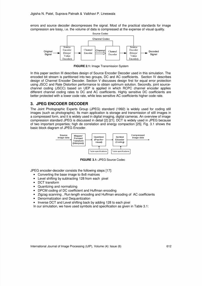
8/6/2019 International Journal of Image Processing (IJIP) Volume 4 Issue 6
http://slidepdf.com/reader/full/international-journal-of-image-processing-ijip-volume-4-issue-6 103/172
Jigisha N. Patel, Suprava Patnaik & Vaibhavi P. Lineswala
International Journal of Image Processing (IJIP), Volume (4): Issue (6) 612
errors and source decoder decompresses the signal. Most of the practical standards for imagecompression are lossy, i.e. the volume of data is compressed at the expense of visual quality.
FIGURE 2.1: Image Transmission System
In this paper section III describes design of Source Encoder Decoder used in this simulation. Theencoded bit stream is partitioned into two groups, DC and AC coefficients. Section IV describesdesign of Channel Encoder Decoder. Section V discusses design first for equal error protectionusing JSCC and Rate Distortion performance to obtain optimum solution. Secondly, joint source-channel coding (JSCC) based on UEP is applied in which RCPC channel encoder appliesdifferent channel coding rates to DC and AC coefficients. Highly sensitive DC coefficients arebetter protected with a lower code rate, while less sensitive AC coefficients higher code rate.
3. JPEG ENCODER DECODERThe Joint Photographic Experts Group (JPEG) standard (1992) is widely used for coding stillimages (such as photographs). Its main application is storage and transmission of still images ina compressed form, and it is widely used in digital imaging, digital cameras. An overview of imagecompression standard JPEG is discussed in detail [2] [21]. DCT is widely used in JPEG becauseof two important properties; high de correlation and energy compaction [25]. Fig. 3.1 shows thebasic block diagram of JPEG Encoder.
FIGURE 3.1: JPEG Source Codec
JPEG encoder-decoder consists the following steps [17]:• Converting the base image to 8x8 matrices• Level shifting by subtracting 128 from each pixel• DCT transform• Quantizing and normalizing• DPCM coding of DC coefficient and Huffman encoding• Zigzag scanning , Run length encoding and Huffman encoding of AC coefficients• Denormalization and Dequantization• Inverse DCT and Level shifting back by adding 128 to each pixelIn our simulation, we have used symbols and specification as given in Table 3.1:
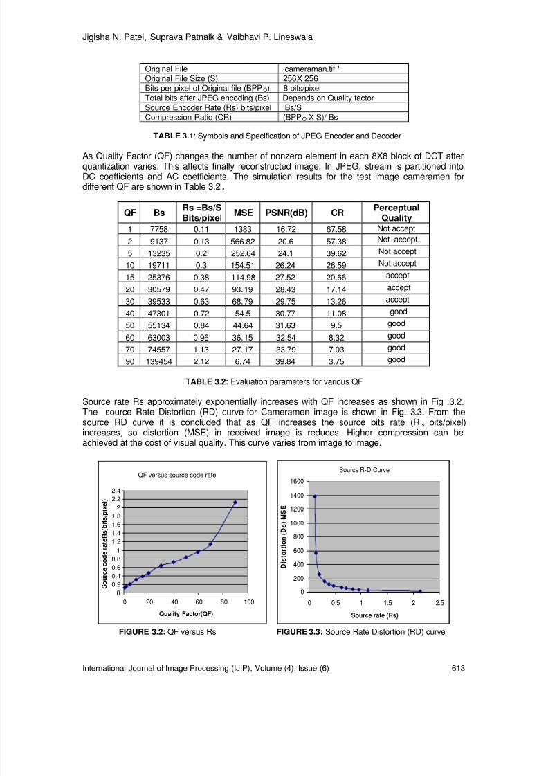
8/6/2019 International Journal of Image Processing (IJIP) Volume 4 Issue 6
http://slidepdf.com/reader/full/international-journal-of-image-processing-ijip-volume-4-issue-6 104/172
Jigisha N. Patel, Suprava Patnaik & Vaibhavi P. Lineswala
International Journal of Image Processing (IJIP), Volume (4): Issue (6) 613
Original File ‘cameraman.tif ‘Original File Size (S) 256 Χ 256Bits per pixel of Original file (BPP O) 8 bits/pixelTotal bits after JPEG encoding (Bs) Depends on Quality factorSource Encoder Rate (Rs) bits/pixel Bs/SCompression Ratio (CR) (BPP O X S)/ Bs
TABLE 3.1 : Symbols and Specification of JPEG Encoder and Decoder
As Quality Factor (QF) changes the number of nonzero element in each 8X8 block of DCT afterquantization varies. This affects finally reconstructed image. In JPEG, stream is partitioned intoDC coefficients and AC coefficients. The simulation results for the test image cameramen fordifferent QF are shown in Table 3.2 .
QF Bs Rs =Bs/SBits/pixel MSE PSNR(dB) CR Perceptual
Quality1 7758 0.11 1383 16.72 67.58 Not accept
2 9137 0.13 566.82 20.6 57.38 Not accept
5 13235 0.2 252.64 24.1 39.62 Not accept
10 19711 0.3 154.51 26.24 26.59 Not accept
15 25376 0.38 114.98 27.52 20.66 accept
20 30579 0.47 93.19 28.43 17.14 accept
30 39533 0.63 68.79 29.75 13.26 accept
40 47301 0.72 54.5 30.77 11.08 good
50 55134 0.84 44.64 31.63 9.5 good
60 63003 0.96 36.15 32.54 8.32 good
70 74557 1.13 27.17 33.79 7.03 good
90 139454 2.12 6.74 39.84 3.75 good
TABLE 3.2: Evaluation parameters for various QF
Source rate Rs approximately exponentially increases with QF increases as shown in Fig .3.2.The source Rate Distortion (RD) curve for Cameramen image is shown in Fig. 3.3. From thesource RD curve it is concluded that as QF increases the source bits rate (R s bits/pixel)increases, so distortion (MSE) in received image is reduces. Higher compression can beachieved at the cost of visual quality. This curve varies from image to image.
QF versus source code rate
0
0.2
0.4
0.6
0.8
11.2
1.4
1.6
1.8
2
2.2
2.4
0 20 40 60 80 100
Quality Factor(QF)
S o u r c e c o
d e r a t e
R s
( b i t s / p i x e l )
Source R-D Curve
0
200
400
600
800
1000
1200
1400
1600
0 0.5 1 1.5 2 2.5
Source rate (Rs)
D i s t o r t i o
n ( D s ) M S E
FIGURE 3.2: QF versus Rs FIGURE 3.3: Source Rate Distortion (RD) curve

8/6/2019 International Journal of Image Processing (IJIP) Volume 4 Issue 6
http://slidepdf.com/reader/full/international-journal-of-image-processing-ijip-volume-4-issue-6 105/172
Jigisha N. Patel, Suprava Patnaik & Vaibhavi P. Lineswala
International Journal of Image Processing (IJIP), Volume (4): Issue (6) 614
4. CHANNEL CODINGThe bit stream for compressed image is more susceptible to channel errors. Thus error controlcoding techniques are used along with compressed image bit stream to minimize the effect ofchannel errors. Various Error Control Techniques are Automatic Repeat Request (ARQ), ForwardError Correction (EFC), Interleaving, Layered Coding with Unequal Error Protection and ErrorConcealment. Cyclic Redundancy Check (CRC-16) code is already proposed for error detection
and Rate Compatible Punctured Convolution (RCPC) [11] [12] [13] [14] code for error correction.When the same protection is given to all encoded source bits regardless their channel errorsensitivity, the method is called Equal Error Protection (EEP). The method of modulating theamount of channel coding based on the required level of protection is known as Unequal ErrorProtection (UEP). UEP scheme allows us to protect significant bits by allocating a lower channelcode rate and less significant bits at a higher channel code rate.
Convolution codes are a powerful class of error correcting codes, providing equal error protectionover the information bit stream [18]. Punctured convolution codes were first introduced by Cain,Clast and Geist [11]. Puncturing is the process of deleting (puncturing) some parity bits from theoutput codeword of lower code rate coder according to a puncturing matrix so that fewer bits aretransmitted than in the original coder and hence leading to higher code rate. For a rate 1/Nmother code rate encoder, the puncturing pattern can be represented as an N x P matrix, where
P is a matrix whose elements are 1’s and 0’s, with a 1 indicating inclusion and a 0 indicatingdeletion of bit. In 1988 Hagenauer [13] extended the concept of punctured convolution codes bypuncturing a low rate 1/N code periodically with period p to obtain a family of codes with rate p/ (p+l) where l can be varied between 1 and (N-1) p .
Fig.4.1 shows convolution code of rate = 1/3 with memory M = 6 and code generator matrix [133171 145]. The specification for RCPC code is given in Table 4.1.
FIGURE 4.1: RCPC Code Generator
TABLE 4.1: Specification of RCPC Code
Mother code rate (1/N) 1/3
PuncturedCode rates,Rc = ( p/p+l)
8/9, 8/10, 812, 8/14, 8/16,
8/18, 8/20, 8/22, 8/24
Puncture period p 8
Decoder Soft decision
Memory 6
Code Generator [133, 171, 145]
Channel type AWGN
Modulation BPSK
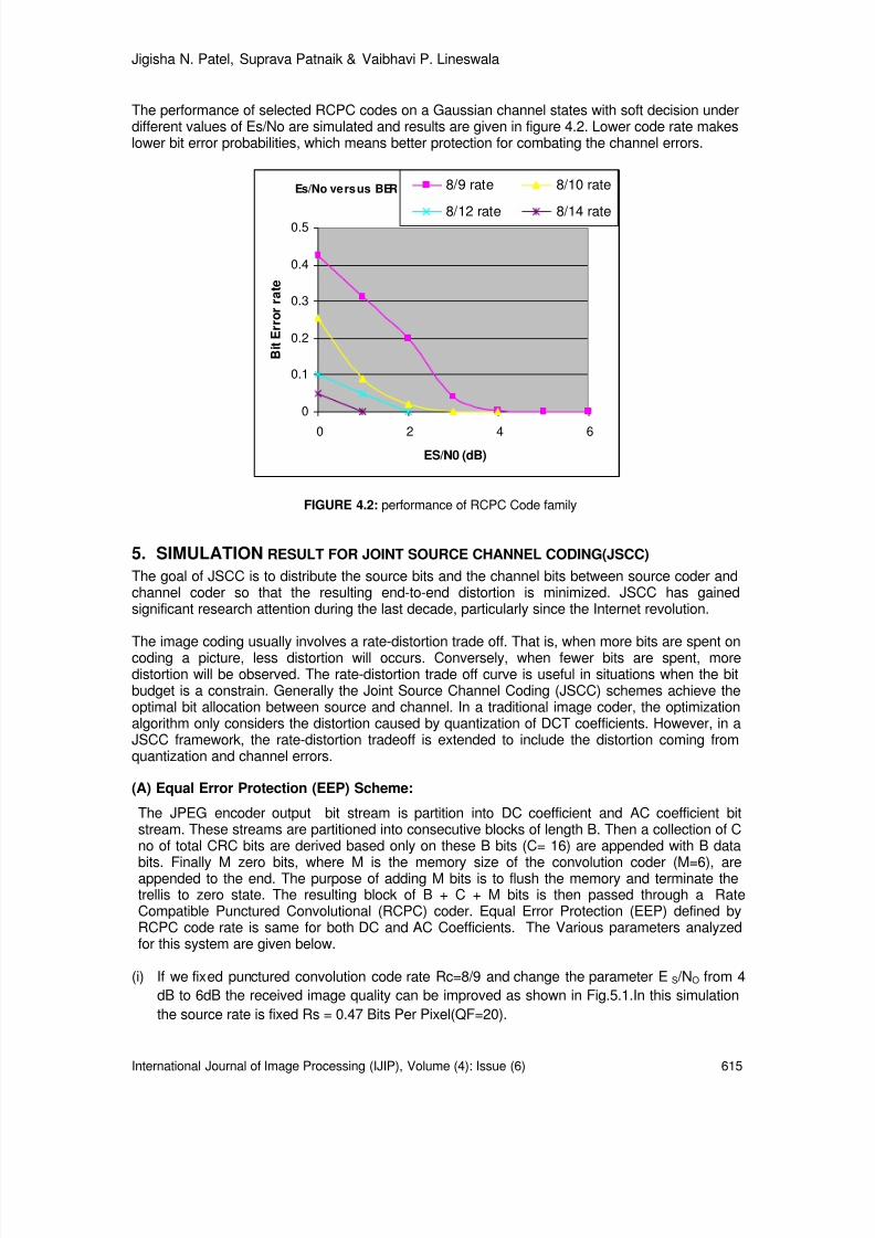
8/6/2019 International Journal of Image Processing (IJIP) Volume 4 Issue 6
http://slidepdf.com/reader/full/international-journal-of-image-processing-ijip-volume-4-issue-6 106/172
Jigisha N. Patel, Suprava Patnaik & Vaibhavi P. Lineswala
International Journal of Image Processing (IJIP), Volume (4): Issue (6) 615
The performance of selected RCPC codes on a Gaussian channel states with soft decision underdifferent values of Es/No are simulated and results are given in figure 4.2. Lower code rate makeslower bit error probabilities, which means better protection for combating the channel errors.
Es/No versus BER
0
0.1
0.2
0.3
0.4
0.5
0 2 4 6
ES/N0 (dB)
B i t E r r o r r a
t e
8/9 rate 8/10 rate
8/12 rate 8/14 rate
FIGURE 4.2: performance of RCPC Code family
5. SIMULATION RESULT FOR JOINT SOURCE CHANNEL CODING(JSCC)The goal of JSCC is to distribute the source bits and the channel bits between source coder andchannel coder so that the resulting end-to-end distortion is minimized. JSCC has gainedsignificant research attention during the last decade, particularly since the Internet revolution.
The image coding usually involves a rate-distortion trade off. That is, when more bits are spent oncoding a picture, less distortion will occurs. Conversely, when fewer bits are spent, moredistortion will be observed. The rate-distortion trade off curve is useful in situations when the bitbudget is a constrain. Generally the Joint Source Channel Coding (JSCC) schemes achieve theoptimal bit allocation between source and channel. In a traditional image coder, the optimizationalgorithm only considers the distortion caused by quantization of DCT coefficients. However, in aJSCC framework, the rate-distortion tradeoff is extended to include the distortion coming fromquantization and channel errors.
(A) Equal Error Protection (EEP) Scheme:
The JPEG encoder output bit stream is partition into DC coefficient and AC coefficient bitstream. These streams are partitioned into consecutive blocks of length B. Then a collection of Cno of total CRC bits are derived based only on these B bits (C= 16) are appended with B data
bits. Finally M zero bits, where M is the memory size of the convolution coder (M=6), areappended to the end. The purpose of adding M bits is to flush the memory and terminate thetrellis to zero state. The resulting block of B + C + M bits is then passed through a RateCompatible Punctured Convolutional (RCPC) coder. Equal Error Protection (EEP) defined byRCPC code rate is same for both DC and AC Coefficients. The Various parameters analyzedfor this system are given below.
(i) If we fixed punctured convolution code rate Rc=8/9 and change the parameter E S /NO from 4dB to 6dB the received image quality can be improved as shown in Fig.5.1.In this simulationthe source rate is fixed Rs = 0.47 Bits Per Pixel(QF=20).

8/6/2019 International Journal of Image Processing (IJIP) Volume 4 Issue 6
http://slidepdf.com/reader/full/international-journal-of-image-processing-ijip-volume-4-issue-6 107/172
Jigisha N. Patel, Suprava Patnaik & Vaibhavi P. Lineswala
International Journal of Image Processing (IJIP), Volume (4): Issue (6) 616
(ii) If we fixed QF =20 and E S /NO=2dB, variation in channel code rate Rc the required bit budgetwill change as given in Table 5.1. Here the simulation is done using fixed packet size 256.Total bit budget at input of channel is defined as R Total .
QF=20, PSNR=19.3918, CR=17.1454 QF=20, PSNR=28.4367, CR=17.1454
FIGURE 5.1: Rate = 8/9 (a) Es/No = 4dB (b) Es/No = 6dB
ChannelCode
Rate(Rc)
PacketLength inBits (B)
TotalPacket(P)=30579/B
TotalBits Bc(Px256)
RTotal =Bc/S
Bits/PixelPSNR Bit Error
Rate(BER)
MSE
8/9 205 150 38400 0.58 4.94 0.2358 2.08E48/10 183 168 43008 0.65 6.66 0.0248 1.4E48/12 149 206 52736 0.8 28.593 0 89.908/14 124 247 63232 0.96 28.593 0 89.908/16 106 289 73984 1.13 28.593 0 89.908/18 92 333 85284 1.3 28.593 0 89.908/20 80 383 98048 1.5 28.593 0 89.908/22 71 431 110336 1.7 28.593 0 89.908/24 64 478 122368 1.87 28.593 0 89.90
TABLE 5.1 QF=20, Es/N0=2dB, packet size 256
As channel code rate reduces, more number of redundancy bits is added. So for fixed QF, bitsper pixel of source (Rs) are fixed, but total transmitted number of bits increasing. As code ratereduces BER performance also improves. At channel code rate (8/12) bit error rate (BER)becomes zero and lower than that the entire code rate, PSNR becomes constant for samechannel condition (E S /NO=2 dB) . This can be considered as optimum channel code rate togenerate highest of PSNR.
(B) Optimum JSCC Design for Fixed bit budget (R Total ) Using RD performance: For fixed total bit rate R Total , EEP algorithm searches all possible combinations of source bit rate(RS) and channel code rate (R C) to find the best one that minimizes the end-to-end distortionDTotal . End to end distortion D Total is measured in terms of Mean Square Error (MSE), it includesboth source distortion and channel distortion. With R Total = 1.5 bits/pixel, Es/No = 2 dB, Packetsize = 256 bits, CRC size = 16 bits, the simulation results are given in Table 5.2 .The operationalRD curve is plotted in Fig. 5.2. Initially as Rs increases, channel code rate is sufficient forcorrecting channel errors up to Rc =8/12. Up to Rc=8/12 rate channel error can be corrected ,sovisual quality improve as Rs increases .But after this point as Rs increases, source distortion
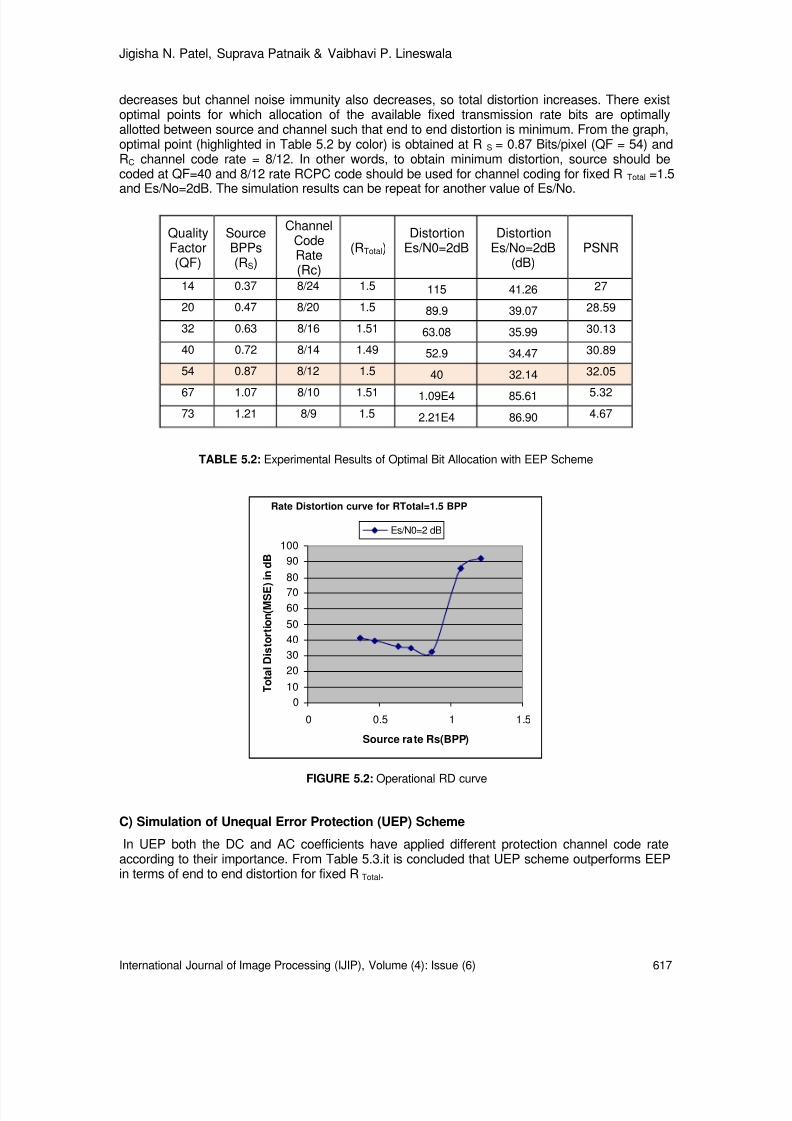
8/6/2019 International Journal of Image Processing (IJIP) Volume 4 Issue 6
http://slidepdf.com/reader/full/international-journal-of-image-processing-ijip-volume-4-issue-6 108/172
Jigisha N. Patel, Suprava Patnaik & Vaibhavi P. Lineswala
International Journal of Image Processing (IJIP), Volume (4): Issue (6) 617
decreases but channel noise immunity also decreases, so total distortion increases. There existoptimal points for which allocation of the available fixed transmission rate bits are optimallyallotted between source and channel such that end to end distortion is minimum. From the graph,optimal point (highlighted in Table 5.2 by color) is obtained at R S = 0.87 Bits/pixel (QF = 54) andRC channel code rate = 8/12. In other words, to obtain minimum distortion, source should becoded at QF=40 and 8/12 rate RCPC code should be used for channel coding for fixed R Total =1.5and Es/No=2dB. The simulation results can be repeat for another value of Es/No.
TABLE 5.2: Experimental Results of Optimal Bit Allocation with EEP Scheme
Rate Distortion curve for RTotal=1.5 BPP
0
10
20
30
40
50
60
70
80
90
100
0 0.5 1 1.5
Source rate Rs(BPP)
T o
t a l D i s t o r t i o n
( M S E ) i n d B
Es/N0=2 dB
FIGURE 5.2: Operational RD curve
C) Simulation of Unequal Error Protection (UEP) Scheme
In UEP both the DC and AC coefficients have applied different protection channel code rateaccording to their importance. From Table 5.3.it is concluded that UEP scheme outperforms EEPin terms of end to end distortion for fixed R Total .
QualityFactor(QF)
SourceBPPs(RS)
ChannelCodeRate(Rc)
(RTotal )Distortion
Es/N0=2dBDistortion
Es/No=2dB(dB)
PSNR
14 0.37 8/24 1.5 115 41.26 27
20 0.47 8/20 1.5 89.9 39.07 28.59
32 0.63 8/16 1.51 63.08 35.99 30.13
40 0.72 8/14 1.49 52.9 34.47 30.89
54 0.87 8/12 1.5 40 32.14 32.05
67 1.07 8/10 1.51 1.09E4 85.61 5.3273 1.21 8/9 1.5 2.21E4 86.90 4.67
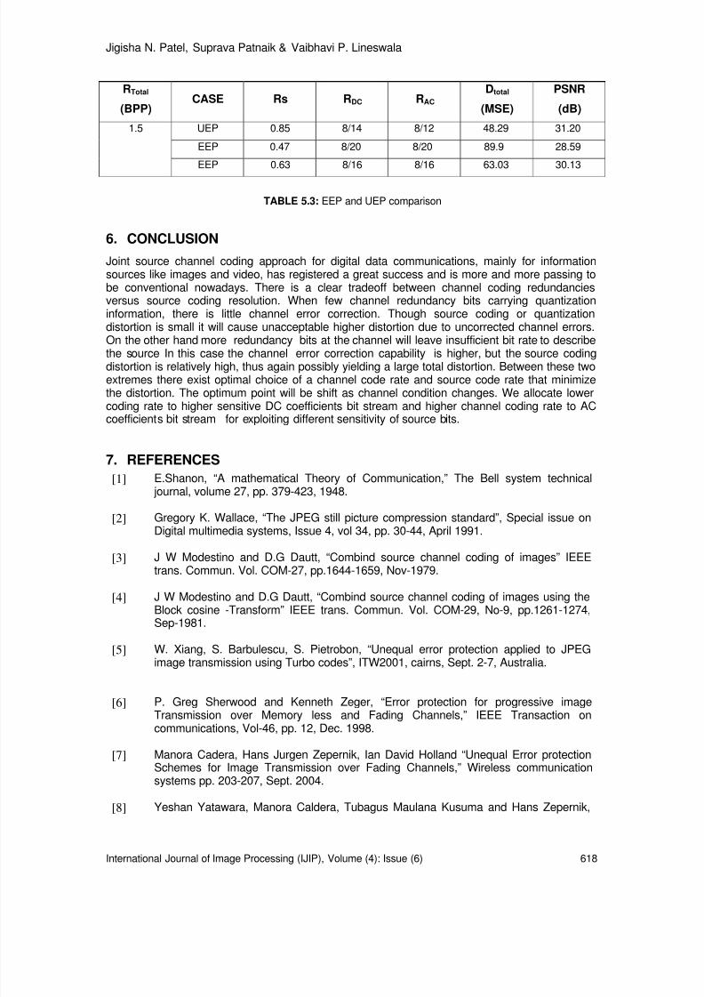
8/6/2019 International Journal of Image Processing (IJIP) Volume 4 Issue 6
http://slidepdf.com/reader/full/international-journal-of-image-processing-ijip-volume-4-issue-6 109/172
Jigisha N. Patel, Suprava Patnaik & Vaibhavi P. Lineswala
International Journal of Image Processing (IJIP), Volume (4): Issue (6) 618
RTotal
(BPP)CASE Rs R DC RAC
Dtotal
(MSE)
PSNR
(dB)
1.5 UEP 0.85 8/14 8/12 48.29 31.20
EEP 0.47 8/20 8/20 89.9 28.59
EEP 0.63 8/16 8/16 63.03 30.13
TABLE 5.3: EEP and UEP comparison
6. CONCLUSION
Joint source channel coding approach for digital data communications, mainly for informationsources like images and video, has registered a great success and is more and more passing tobe conventional nowadays. There is a clear tradeoff between channel coding redundanciesversus source coding resolution. When few channel redundancy bits carrying quantizationinformation, there is little channel error correction. Though source coding or quantizationdistortion is small it will cause unacceptable higher distortion due to uncorrected channel errors.On the other hand more redundancy bits at the channel will leave insufficient bit rate to describethe source In this case the channel error correction capability is higher, but the source codingdistortion is relatively high, thus again possibly yielding a large total distortion. Between these twoextremes there exist optimal choice of a channel code rate and source code rate that minimizethe distortion. The optimum point will be shift as channel condition changes. We allocate lowercoding rate to higher sensitive DC coefficients bit stream and higher channel coding rate to ACcoefficients bit stream for exploiting different sensitivity of source bits.
7. REFERENCES[1] E.Shanon, “A mathematical Theory of Communication,” The Bell system technical
journal, volume 27, pp. 379-423, 1948.
[2] Gregory K. Wallace, “The JPEG still picture compression standard”, Special issue onDigital multimedia systems, Issue 4, vol 34, pp. 30-44, April 1991.
[3] J W Modestino and D.G Dautt, “Combind source channel coding of images” IEEEtrans. Commun. Vol. COM-27, pp.1644-1659, Nov-1979.
[4] J W Modestino and D.G Dautt, “Combind source channel coding of images using theBlock cosine -Transform” IEEE trans. Commun. Vol. COM-29, No-9, pp.1261-1274,Sep-1981.
[5] W. Xiang, S. Barbulescu, S. Pietrobon, “Unequal error protection applied to JPEGimage transmission using Turbo codes”, ITW2001, cairns, Sept. 2-7, Australia.
[6] P. Greg Sherwood and Kenneth Zeger, “Error protection for progressive imageTransmission over Memory less and Fading Channels,” IEEE Transaction oncommunications, Vol-46, pp. 12, Dec. 1998.
[7] Manora Cadera, Hans Jurgen Zepernik, Ian David Holland “Unequal Error protectionSchemes for Image Transmission over Fading Channels,” Wireless communicationsystems pp. 203-207, Sept. 2004.
[8] Yeshan Yatawara, Manora Caldera, Tubagus Maulana Kusuma and Hans Zepernik,

8/6/2019 International Journal of Image Processing (IJIP) Volume 4 Issue 6
http://slidepdf.com/reader/full/international-journal-of-image-processing-ijip-volume-4-issue-6 110/172
Jigisha N. Patel, Suprava Patnaik & Vaibhavi P. Lineswala
International Journal of Image Processing (IJIP), Volume (4): Issue (6) 619
“Unequal Error protection for ROI Coded Images over Fading Channels” IEEEProceedings of the system Communications, pp. 111-115, Aug. 2005.
[9] Pasteur Poda and Ahmed Tamtaoui, “On the Enhancement of Unequal ErrorProtection Performance in Images Transmission Over Time Varying Channels,”IJCSNS International Journal of Computer Science and Network Security, Vol. 6, No.9B, Sept. 2006.
10] Chou-Chen Wang, Tung-Yuen Huang and chung You Yang, “Joint Source ChannelCoding for JPEG Compressed Images over Noisy Channel,” Congress on Image andSignal Processing, IEEE Computer society pp. 676-680, 2008.
11] J.B.Cain, G.C Clark, and J M Geist,” Punctured convolutional codes of rate (n-1)/n andsimplified maximum likelihood decoding” IEEE Tran. Inform. Theory, vol.IT-20, pp.388-389, May 1974.
12] Y. Yasuda et al., “High rate punctured convolution codes for soft decision viterbidecoding”, IEEE Trans. Commu., vol. COM-32, pp. 315-319, Mar.1984.
13] J. Hagenauer, “Rate compatible punctured convolutional codes (RCPC) and theirapplication” IEEE transaction on communication vol 36 no 4, pp. 389-400, April 1988.
14] A. J. Viterbi, “Convolutional codes and their performance in communication systems”IEEE Trans Commun. Technol., vol. COM-19, pp.751-772, OCT-1971.
15] M.J. uf and J.W. Modestimo, ”Operational Rate Distortion performance for joint sourceand channel coding of images” IEEE Trans Image processing, vol. -8, pp.68-84, Mar1999.
16] B. Hochwald and K. zegar, “Tradeoff between source and channel coding. ‘IEEE TransInformation theory, vol.43, Sept 1997.
17] Rafael C. Gonzalez & Richard E. Woods, “Digital Image Processing”, second edition,Pearson Education publication, 2002.
18] Sklar, B., “Digital Communications: Fundamentals and Applications”, Second Edition,Prentice-Hall, pp 436-460, 2001
19] K. R. Rao, N. Ahmed, T. Natarajan “Discrete Cosine Transform”, IEEE transactionscomputers, vol. 23, pp. 90-93, Jan 1974.
20] Zhenyu Wu, “Joint source channel coding for image transmission with JPEG200 overmemoryless channels”, IEEE transactions on image processing, vol. 14, no. 8, pp1020-1032, Aug 2005.
21] Navin Chaddha and Suhas Diggavi, “A Frame-work for Joint Source-Channel Codingof Images over Time-Varying Wireless Channels”, IEEE xplore, pp 89-92, 1996.

8/6/2019 International Journal of Image Processing (IJIP) Volume 4 Issue 6
http://slidepdf.com/reader/full/international-journal-of-image-processing-ijip-volume-4-issue-6 111/172
Dr. H.B. Kekre, Sudeep Thepade & Shrikant Sanas
International Journal of Image Processing (IJIP), Volume (4): Issue (6) 620
Improving Performance of Multileveled BTC Based CBIR UsingSundry Color Spaces
Dr. H. B. Kekre [email protected] Professor,
MPSTME, SVKM’s NMIMS University,Mumbai-56, India
Sudeep Thepade [email protected] Associate Professor and Ph.D. Research Scholar,MPSTME,SVKM’s NMIMS University,Mumbai-56, India
Shrikant P. Sanas [email protected] Student MPSTME,SVKM’s NMIMS University,Mumbai-56, India
Abstract
The paper presents an extension of content based image retrieval (CBIR)techniques based on multilevel Block Truncation Coding (BTC) using nine sundrycolor spaces. Block truncation coding based features is one of the CBIR methodsproposed using color features of image. The approach basically considers red,green and blue planes of an image to compute feature vector. This BTC basedCBIR can be extended as multileveled BTC for performance improvement inimage retrieval. The paper extends the multileveled BTC using RGB color spaceto other nine color spaces. The CBIR techniques like BTC Level-1, BTC Level-2,BTC Level-3 and BTC Level-4 are applied using various color spaces to analyzeand compare their performances. The CBIR techniques are tested on genericimage database of 1000 images spread across 11 categories. For each CBIRtechnique, 55 queries (5 per category) are fired on extended Wang genericimage database to compute average precision and recall for all queries. Theresults have shown the performance improvement (ie., higher precision andrecall values) with BTC-CBIR methods using luminance-chrominance colorspaces (YCgCb, Kekre’s LUV, YUV, YIQ, YCbCr) as compared to non-luminance (RGB, HSI, HSV, rgb , XYZ) Color spaces. The performance ofmultileveled BTC-CBIR increases gradually with increase in level up to certainextent (Level 3) and then increases slightly due to voids being created at higherlevels. In all levels of BTC Kekre’s LUV color space gives best performance.
Keywords: Content Based Image Retrieval (CBIR), BTC, Color Spaces.
1. INTRODUCTION
From ancient era, images play an important role in human communication. It is basic andcommon way to express the information. Today with advancement in information and

8/6/2019 International Journal of Image Processing (IJIP) Volume 4 Issue 6
http://slidepdf.com/reader/full/international-journal-of-image-processing-ijip-volume-4-issue-6 112/172
Dr. H.B. Kekre, Sudeep Thepade & Shrikant Sanas
International Journal of Image Processing (IJIP), Volume (4): Issue (6) 621
communication technology most of the information is digitized. Large amount of digital data isgenerated, transmitted, stored, analyzed and accessed. Mostly, information is in the form ofmultimedia such as digital images, audio, video, graphics [6]-8. Large numbers of images aregenerated from various sources on a daily basis. Such images occupy lot of space and are verychallenging to search and retrieve from very large image pool. The need for efficient retrieval ofimages has been recognized by managers and users of large image collections. Efficient indexingtechniques for the retrieval of best matching image from a huge database of images are beingdeveloped. Content based image retrieval gives efficient solution to these problems [18,19].Content Based Image Retrieval (CBIR) is used to provide a high percentage of relevant images inresponse to the query image [12]. The goal of an image retrieval system is to retrieve a set ofmatching images from an image database [21].
A Content Based Image Retrieval (CBIR) technique takes an image as an input to query andoutputs number of matching images to the query image [11]. In CBIR technique, features areused to represent the image content. The features are extracted automatically and there is nomanual intervention, and thus eliminating the dependency on humans in the feature extractionstage [10]. The typical CBIR system performs two major tasks. The first one is feature extraction(FE), where a set of features, forming feature vector, is generated to accurately represent thecontent of each image in the database. A feature vector is much smaller in size than the originalimage. The second task is similarity measurement (SM), where a distance between the queryimage and each image in the database using their feature vectors (signatures) is computed sothat the top “closest” images retrieved [3], [13], [14], [15].
Many current CBIR system use Euclidean distance [5] on the extracted feature set as a similaritymeasure. The Direct Euclidian distance between image P and query image Q can be given asequation. where Vpi and Vqi are the feature vectors of image P and query image Q respectivelywith size ‘n’.
∑=
−=
n
iVqiVpi ED
1
2
)( (1)
Some of important applications for CBIR technology could be identified as art galleries,museums, archaeology, architecture design, geographic information systems, weather forecast,
medical imaging , trademark databases, criminal investigations, image search on the Internet.The thirst of a better and faster image retrieval technique is increasing day by day. The paperdiscusses the performance improvement in multileveled BTC based CBIR techniques [1] usingvarious color spaces. In all ten different color spaces including RGB color space are consideredhere with four different levels of BTC for feature extraction resulting into total 40 CBIR methods.
2. BLOCK TRUNCATION CODING (BTC) Block truncation coding (BTC) is a relatively simple image coding technique developed in theearly years of digital imaging more than 29 years ago. Although it is a simple technique, BTC hasplayed an important role in the history of digital image coding in the sense that many advancedcoding techniques have been developed based on BTC or inspired by the success of BTC [2].Block Truncation Coding (BTC) was first developed in 1979 for grayscale image coding [2]. The
method first computes the mean pixel value of the whole block and then each pixel in that block iscompared to the block mean. If a pixel is greater than or equal to the block mean, thecorresponding pixel position of the bitmap will have a value of 1 otherwise it will have a value of 0.Two mean pixel values one for the pixels greater than or equal to the block mean and the otherfor the pixels smaller than the block mean are also calculated. At decoding stage, the smallblocks are decoded one at a time. For each block, the pixel positions where the correspondingbitmap has a value of 1 is replaced by one mean pixel value and those pixel positions where thecorresponding bitmap has a value of 0 is replaced by another mean pixel value.

8/6/2019 International Journal of Image Processing (IJIP) Volume 4 Issue 6
http://slidepdf.com/reader/full/international-journal-of-image-processing-ijip-volume-4-issue-6 113/172
Dr. H.B. Kekre, Sudeep Thepade & Shrikant Sanas
International Journal of Image Processing (IJIP), Volume (4): Issue (6) 622
3. CBIR USING MULTILEVELED BLOCK TRUNCATION CODINGThe block truncation coding (BTC) technique can be extended to higher levels by consideringmultiple threshold values to divide the image pixels into higher (upper) and less than or equal to(lower) threshold. The image pixel data is thus divided in to multiple clusters and per cluster themean value is taken as part of feature vector. At BTC Level 1 only one threshold value is used todivide the pixel data to get two clusters and respective means of these clusters as upper meanand lower mean are computed, resulting in to feature vector of size six (two values per colorplane). In next level each cluster can be further divided into two parts with respect to it’s meanvalue resulting into total four clusters per color plane to get feature vector of size twelve (four perplane). Thus BTC can be extended to multiple levels to get BTC Level 2, BTC Level 3, etc. Thefeature vector extraction for CBIR using multileveled BTC with RGB color space is explained insection A, B and C here.
A) CBIR using BTC-RGB-Level-1 (BTC-RGB-6) [3,4,9,17]
In original BTC we divide the image into R, B, and G components and compute the mean value ofeach color component as individual color. Let I(m,n)=[R(m,n), G(m,n), B(m,n)] be the color imageimage of size mxn. Let the thresholds be MR, MG and MB, which could be computed as per theequations 2, 3 and 4.
∑∑= =
=m
i
n
j
ji Rnm
MR1 1
),(*1 (2)
∑∑
= =
=
m
i
n
j
jiGnm
MG1 1
),(*1
(3)
∑∑
= =
=
m
i
n
j
ji Bnm
MB1 1
),(*1
(4)
Here three binary bitmaps will be computed as BMr, BMg and BMb. If a pixel in each component
(R, G, and B) is greater than or equal to the respective threshold, the corresponding pixel positionof the bitmap will have a value of ‘1’ otherwise it will have a value of ‘0’.
MR ji Rif
MR ji Rif
ji BMr <=
>
=
),(...,....0
),(....,1
),( (5)
MG jiGif
MG jiGif
ji BMg<=
>
=
),(...,....0
),(....,1
),( (6)
MB ji Bif
MB ji Bif
ji BMb
<=
>
=
),(...,....0
),(....,1
),( (7)
),(*),(*),(
1
1 1
1 1
ji R ji BMr ji BMr
URm
i
n
jm
i
n
j
∑ ∑∑ ∑ = =
= =
=
(8)

8/6/2019 International Journal of Image Processing (IJIP) Volume 4 Issue 6
http://slidepdf.com/reader/full/international-journal-of-image-processing-ijip-volume-4-issue-6 114/172
Dr. H.B. Kekre, Sudeep Thepade & Shrikant Sanas
International Journal of Image Processing (IJIP), Volume (4): Issue (6) 623
Two mean colors one for the pixels greater than or equal to the threshold and other for the pixelssmaller than the threshold are also calculated [15]. The upper mean color UM(UR, UG, UB) isgiven as equations 8, 9 and 10.
And the Lower Mean LM= (LR, LG, LB) is computed as following equations 11, 12 and 13.
),(*),(1*),(*
1
1 1
1 1
ji R ji BMr ji BMr nm
LRm
i
n
jm
i
n
j
∑∑∑∑ = =
= =
−
−
=
(11)
),(*),(1*),(*
1
1 1
1 1
jiG ji BMg ji BMgnm
LGm
i
n
jm
i
n
j
∑∑∑∑ = =
= =
−
−
=
(12)
),(*),(1*),(*
1
1 1
1 1
ji B ji BMb ji BMbnm
LBm
i
n
jm
i
n
j
∑∑∑∑ = =
= =
−
−
=
(13)
These Upper Mean and Lower Mean together will form a feature vector or signature of the image.For every image stored in the database these feature vectors are computed and stored in featurevector table.
B) CBIR using BTC- RGB- Level 2 (BTC-RGB-12)[1]
In BTC-RGB-Level 2 the image data is divided into 12 parts using the six means obtained in BTC-RGB-Level 1. Here the bitmap are prepared using upper and lower mean values of individual
color components. For red color component the bitmap ‘BMUR’ and ‘BMLR’ are generated asgiven in equations 14 and 15. Similarly for green color component ‘BMUG’ & ‘BMLR’ and for bluecolour components ‘BMUB’ & ‘BMLB’ can be generated.
UR ji Rif
UR ji Rif
ji BMUR<=
>
=
),(...,....0
),(....,1
),( (14)
LR ji Rif
LR ji Rif
ji BMLR<=
>
=
),(...,....0
),(....,1
),( (15)
Using this bitmap the two mean colour per bitmap one for the pixels greater than or equal to thethreshold and other for the pixels smaller than the threshold are calculated [15]. The red plane ofthe image is divided into two parts as upper red image and lower red image as given byequations 16 and 17.
....1.,...1.),..,(*),(),( n jand mi for ji BMr ji R ji Iur === (16)
....1.,...1.)],..,(1[*),(),( n jand mi for ji BMr ji R ji Ilr ==−= (17)
),(*),(*),(
1
1 1
1 1
jiG ji BMg ji BMg
UGm
i
n
jm
i
n
j
∑ ∑∑∑ = =
= =
=
(9)
),(*),(*),(
1
1 1
1 1
ji B ji BMb ji BMb
UBm
i
n
jm
i
n
j
∑ ∑∑ ∑ = =
= =
=
(10)

8/6/2019 International Journal of Image Processing (IJIP) Volume 4 Issue 6
http://slidepdf.com/reader/full/international-journal-of-image-processing-ijip-volume-4-issue-6 115/172
Dr. H.B. Kekre, Sudeep Thepade & Shrikant Sanas
International Journal of Image Processing (IJIP), Volume (4): Issue (6) 624
The upper mean color UM (UUR, ULR, UUG, ULG, UUB, ULB) are given as follows.
),(*),(*),(
1
1 1
1 1
ji Iur ji BMUR ji BMUR
UURm
i
n
jm
i
n
j
∑ ∑∑ ∑ = =
= =
=
(18)
),(*),(*),(
1
1 1
1 1
ji Ilr ji BMLR ji BMLR
ULR
m
i
n
jm
i
n
j
∑ ∑∑ ∑ = =
= =
=
(19)
And the first two components of Lower Mean LM= (LUR, LLR, LUG, LLG, LUB, LLB) arecomputed using following equations
),(*),(1*),(
1
1 1
1 1
ji Iur ji BMUR ji BMUR
LURm
i
n
jm
i
n
j
∑∑∑∑ = =
= =
−=
(20)
),(*),(1*),(
1
1 1
1 1
ji Ilr ji BMLR ji BMLR
LLRm
i
n
jm
i
n
j
∑∑∑∑ = =
= =
−=
(21)
These Upper Mean and Lower Mean values together will form a feature vector for BTC-12. Forevery image stored in the database these feature vectors are computed and stored in featurevector table.
C) CBIR using BTC-RGB-Level 3 (BTC-RGB-24)[1] and BTC-RGB-Level 4 (BTC-RGB-48)Similarly the feature vector for BTC-24 can be found by extending the BTC till level 3. Each planewill give the 8 elements of feature vector. For Red plane we get (UUUR, LUUR, ULUR, LLUR,UULR, LULR, ULLR, LLLR). Also feature vector of size 48 can be generated by extending thisprocess of BTC to next level.
4. COLOR SPACES IN CBIR USING MULTILEVELED BTCJust as discussed in section 3 for RGB color space, the CBIR using multileveled BTC can beused with other color spaces. Here in all ten color spaces like RGB, HSV[20], XYZ[20], rgb[20],HSI[20], Kekre’s LUV [3], YCbCr[17], YUV[9], YIQ[20], Kekre’s YCgCb[20] are considered. Theten color spaces along with BTC extended to four levels resul into total 40 CBIR methods. Thesecolor spaces can mainly be divided into two categories as luminance-chrominance color spaces(Kekre’s LUV, YCbCr, YUV, YIQ, Kekre’s YCgCb) and nom-luminance color spaces (RGB, HSI,HSV, XYZ and rgb).
5. IMPLEMENTATION The implementation of these CBIR techniques is done using MATLAB 7.0. The CBIR techniquesare tested on the augmented Wang [15] image database of 1000 variable size images spreadacross 11 categories of human beings, animals, natural scenery and man-made things. To
compare various techniques in various color space, performance is evaluated based on precisionand recall. The efficiency of CBIR technique is evaluated based on accuracy, stability and speed.To assess the retrieval effectiveness, we have used the precision and recall as statisticalcomparison parameters for the BTC-6, BTC-12, BTC-24 and BTC-48 techniques of CBIR on allcolor spaces. The standard definitions of these two measures are given by following equations.
edes_retriever_of_imagTotal_numbievedmages_retrrelevant_iNumber_of_
Precesion = (22)

8/6/2019 International Journal of Image Processing (IJIP) Volume 4 Issue 6
http://slidepdf.com/reader/full/international-journal-of-image-processing-ijip-volume-4-issue-6 116/172

8/6/2019 International Journal of Image Processing (IJIP) Volume 4 Issue 6
http://slidepdf.com/reader/full/international-journal-of-image-processing-ijip-volume-4-issue-6 117/172
Dr. H.B. Kekre, Sudeep Thepade & Shrikant Sanas
International Journal of Image Processing (IJIP), Volume (4): Issue (6) 626
FIGURE 1 : Precision & Recall plotted against for RGB color space.
FIGURE2.A: Crossover points of Precision-Recall plotted against number of retrieved images.
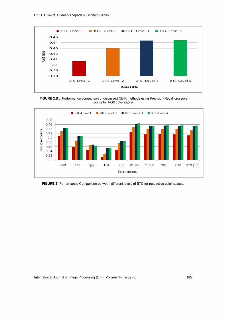
8/6/2019 International Journal of Image Processing (IJIP) Volume 4 Issue 6
http://slidepdf.com/reader/full/international-journal-of-image-processing-ijip-volume-4-issue-6 118/172
Dr. H.B. Kekre, Sudeep Thepade & Shrikant Sanas
International Journal of Image Processing (IJIP), Volume (4): Issue (6) 627
FIGURE 2.B : Performance comparison of discussed CBIR methods using Precision-Recall crossoverpoints for RGB color sapce.
FIGURE 3: Performance Comparison between different levels of BTC for respective color spaces.

8/6/2019 International Journal of Image Processing (IJIP) Volume 4 Issue 6
http://slidepdf.com/reader/full/international-journal-of-image-processing-ijip-volume-4-issue-6 119/172
Dr. H.B. Kekre, Sudeep Thepade & Shrikant Sanas
International Journal of Image Processing (IJIP), Volume (4): Issue (6) 628
FIGURE 4: Performance Comparison between different color spaces for respective level of BTC.
7. CONCLUSIONThe performance of CBIR system depends on the precision and recall. Quite often the crossoverpoint of precision and recall is taken as criteria for judging the performance of CBIR technique onvarious Color spaces. Kekre’s LUV gives better result and the values are 0.4258, 0.448, 0.462,0.46495 for BTC-6, BTC-12, BTC-24 and BTC-48 respectively. The results have shown that, theperformance improvement (i.e. higher precision and recall values) in Luminous & ChrominanceColor spaces with BTC-CBIR methods compared to Non-Luminous &Non-Chrominance Colorspaces are lower. Performance improves with increased level of BTC. Up to level -3 gradualincreases in performance with increasing level is observed while the difference of performance inlevel-3 and level-4 is negligible due to voids being created at higher levels.
8. REFERENCES[1] Dr.H.B.Kekre, Sudeep D. Thepade, Shrikant P. Sanas ‘Improved CBIR using Multileveled
Block Truncation Coding’ International Journal of Computer Science and Engineering(IJCSE), Volume 2, Number 7, October 2010 Edition, pp2471-2476.http://www.enggjournals.com/ijcse .
[2] Guoping Qiu, “Color Image Indexing Using BTC,” IEEE Transactions on Image Processing,VOL.12, NO.1, pp.93-101, January 2003.
[3] Dr.H.B.Kekre, Sudeep D. Thepade, “Boosting Block Truncation Coding using Kekre’s LUVColor Space for Image Retrieval”, WASET International Journal of Electrical, Computer andSystem Engineering (IJECSE), Volume 2, Number 3, pp. 172-180, Summer 2008. Availableonline at http://www.waset.org/ijecse/v2/v2-3-23.pdf
[4] Dr.H.B.Kekre, Sudeep D. Thepade, “Image Retrieval using Augmented Block TruncationCoding Techniques”, ACM International Conference on Advances in Computing,Communication and Control (ICAC3-2009), pp. 384-390, 23-24 Jan 2009, Fr. ConceicaoRodrigous College of Engg., Mumbai. Is uploaded on online ACM portal.
[5] Dr.H.B.Kekre, Sudeep D. Thepade, “Scaling Invariant Fusion of Image Pieces in PanoramaMaking and Novel Image Blending Technique”, International Journal on Imaging (IJI),www.ceser.res.in/iji.html, Volume 1, No. A08, pp. 31-46, Autumn 2008.

8/6/2019 International Journal of Image Processing (IJIP) Volume 4 Issue 6
http://slidepdf.com/reader/full/international-journal-of-image-processing-ijip-volume-4-issue-6 120/172

8/6/2019 International Journal of Image Processing (IJIP) Volume 4 Issue 6
http://slidepdf.com/reader/full/international-journal-of-image-processing-ijip-volume-4-issue-6 121/172

8/6/2019 International Journal of Image Processing (IJIP) Volume 4 Issue 6
http://slidepdf.com/reader/full/international-journal-of-image-processing-ijip-volume-4-issue-6 122/172
Innchyn HER, Kazi Mostafa & Huan-Kai Hung
International Journal of Image Processing (IJIP), Volume (4): Issue (6) 631
A Hybrid Trademark Retrieval System Using Four-Gray-LevelZernike Moments and Image Compactness Indices
Innchyn Her [email protected] Professor, Dept. of Electro-mechanical Engineering National Sun Yat-sen University Kaohsiung 80424, Taiwan
Kazi Mostafa [email protected], Dept. of Electro-mechanical Engineering National Sun Yat-sen University Kaohsiung 80424, Taiwan
Huan-Kai Hung [email protected], Dept. of Electro-mechanical Engineering National Sun Yat-sen University
Kaohsiung 80424, Taiwan
Abstract
There are just too many trademarks out there so that a good automated retrievalsystem is required to help to protect them from possible infringements. However,it is from people, i.e., the general consumers' viewpoint how similar or confusingtwo trademarks can be. Thus, in this paper we propose a hybrid system wherewe patently incorporate human inputs into a computerized trademark retrievalscheme. Various surveys involving general consumers' cognition and responsesare conducted, and the results are used as benchmarks in developing theautomated part. The core mathematical features used in the scheme are four-gray-level Zernike moments and two new image compactness indices.Experimental results show that this hybrid system, when compared with human-generated results, is able to achieve an average accuracy rate of 95% while thatof the closest competing existing method is 65%.
Keywords: Image matching, Information retrieval, Trademarks.
1. INTRODUCTION
Owing to the constant development of commercial activities the number of trademarks used bycompanies increases dramatically by the year. Consequently, to design a new trademark withoutinfringing others has become a critical and complex issue. With the advent of computers,traditional ways of archiving many documents have been replaced by computerized methods,which feature automated processes and fast and accurate information retrieval. When it comes totrademarks, unfortunately, there is no universally accepted sorting and retrieval scheme so far.For instance, through keywords or search codes that are manually assigned to the trademarkimages, an official retrieval system has been used for some time [1][22]. This procedure, thoughfeasible, contains major drawbacks. It is very difficult for an operator to describe all images evenlyobjectively and consistently, especially for abstract or complex ones and over a long period of

8/6/2019 International Journal of Image Processing (IJIP) Volume 4 Issue 6
http://slidepdf.com/reader/full/international-journal-of-image-processing-ijip-volume-4-issue-6 123/172
Innchyn HER, Kazi Mostafa & Huan-Kai Hung
International Journal of Image Processing (IJIP), Volume (4): Issue (6) 632
time. On the other hand, a different approach called Content-Based Image Retrieval (CBIR)proposes an image-based strategy instead of a tag-based one. Each trademark is processedbeforehand, to leave and save its pertinent features in the computer. Then for a new trademarkapplication, the features of the new image are compared with the stored data to see if there havebeen similar entries in the database. Such CBIR trademark retrieval systems are intrinsically lesssusceptible to human errors. A good CBIR scheme tends to exhibit robustness in terms of imagesize, position, and orientation variations. In general, these methods are often classified intocontour-based schemes and region-based schemes.
A very early effort to digitally define the features of an image was the work by Freeman [2]. Heinvented the chain code, a typical contour-based approach. Many researchers later refined hismethod to improve the applicability. For example, Peng and Chen [3] more recently proposed touse the chain code to describe simple and properly segmented trademarks, while encoding themaccording to the angles. Contour-based methods are usually for simple, binary images. Anadvantage is that the coded contour is usually invariant with respect to translation and rotation [4].Yet the newer region-based methods have a broader application range and a larger toolbox touse. For example, there are moments of various kinds, often used as descriptive features of animage. A benefit of using the moments is their insensitivity to noise. As a result, researchers havebegun to resort more to region-based techniques in these years. For instance, Yin and Yeh [5]have proposed a method to employ a fuzzy approach to expedite the image classifying andretrieval processes. The image features used were the area, the number of closed objects, thelocation of the centroid, and symmetry of the image, etc.
The invariant moments, devised by Hu [6] based on geometric moments, have long been valuedas useful image descriptive features. But they are comparatively sensitive to noise and theaccompanying image reconstruction procedure was difficult. Shih and Chen [7] later suggested touse invariant moments with Fourier transforms and the histogram of image boundary orientationsas features in a trademark retrieval scheme. Ciocca and Schettini [8] also demonstrated a way forsmartly using the invariant moments. They combined moments with boundary directions and theresults from a multi-resolution wavelet transform. Through a relevance feedback scheme theycould compute the similarity between trademarks. On the other hand, there were researcherswho had chosen to use Zernike moments for trademark retrieval schemes. For example, Kim andKim [9] constructed a Gamma distribution model with Zernike moments to describe visually
salient features of monochrome trademarks. Subsequently, Kim et al. [10] also presented amodified Zernike-moment shape descriptor, by first partitioning a trademark image into an innerand an outer region. More recently, Kamila et al. [11] normalized the regular Zernike moments viageometric moments and used them with binary images.
Regardless of these many research efforts on automated trademark retrieval methodology, thegoverning institution that supervises the examination and approval of trademarks still, for the timebeing, relies largely on manual and tag-based methods [1], [12], [13], [14]. From scientific point ofview, a trademark is invariably an image, a discrete two-dimensional mathematical function.Using search codes to describe and to retrieve an image risks the danger of inaccuracy,inconsistency, and inefficiency. But why do people still stick to them? One blunt answer:Undeniably, trademark is not an engineering or scientific term. It is purely commercial;trademarks are meant to interact with people. They contain subtle feelings difficult to perceive or
describe by the computer. For the task of trademark comparison and retrieval, human inputs cannever be dismissed.
In light of this we now propose a hybrid retrieval system for trademarks. In the core of ournumerical scheme, we use Zernike moments for their resistance to noise, their invariance torotation, and multi-resolution capabilities. Besides, two new image features are proposed asadditional sorting criteria for the computer. However, the term "hybrid" implies that humanperception works hand in hand with computer's speed. In this system humans set up abenchmark while the computer emulates humans' cognition and feeds back a list of candidates

8/6/2019 International Journal of Image Processing (IJIP) Volume 4 Issue 6
http://slidepdf.com/reader/full/international-journal-of-image-processing-ijip-volume-4-issue-6 124/172
Innchyn HER, Kazi Mostafa & Huan-Kai Hung
International Journal of Image Processing (IJIP), Volume (4): Issue (6) 633
for human to make final judgments. We will show that the hybrid system is robust and able toprovide an output very usable for a professional trademark examiner.
2. PRELIMINARIES2.1 Trademarks
A trademark is a mark that identifies one person's goods [13]. In practice, the word "trademark" isused to refer to any class of mark, or a word, symbol, or phrase, used to distinguish a particularmanufacturer's product from those of others. The enactment of the trademark law aims to protectthe legal use of the trademarks, so that legitimate transactions and fair business morals areguaranteed. It is obvious that there is little room for confusion in the use of trademarks. However,if there is any, in particular deliberate confusion, an act of infringement is very likely evolvingsomewhere.
Thanks to the collaborated efforts of industrialized nations and the WTO, trademark definition andlaws around the world are quite similar now. According to a typical trademark regulation [14],there are four different kinds of trademarks, as depicted in Fig. 1. In this paper, we will dealmostly with graph and sign trademarks for they are more difficult to describe in words.
There are a few rules in determining the similarity of trademarks. The most important aspect isthe impression the whole trademark imposes on the consumers. It is by this crude totalimpression that people decide whether two trademarks are confusingly similar or not. Asconfirmed by a senior officer of local Patent and Trademark Office [15], people are moreimpressed by the rough shape of a trademark, rather than by its details or color. Moreover,people tend to neglect the frame or circle outside the trademark. For computers, a framedtrademark can be a far cry from an unframed one. For people, strangely, they produce almostidentical impressions.
FIGURE 1: Different kinds of trademarks: (a) Word trademarks, (b) Graph trademarks,(c) Sign trademarks, and (d) Combined trademarks.
To verify the above statements, we have conducted a questionnaire survey that involved 100general consumers [16]. When presented with a single trademark design, 59 consumers said thatthe color was the most impressing feature, versus 34 for the shape and 5 for its pronunciation.However, when presented with sets of similar trademarks for comparison, a total of 83 consumersconfirmed that the rough shapes of the trademarks, rather than their colors or details, were themost discerning feature for trademark identification. In view of this double testimony, we decidedto devise two new features solely for the rough shape of the trademark image. They will bediscussed in Section 3.2.

8/6/2019 International Journal of Image Processing (IJIP) Volume 4 Issue 6
http://slidepdf.com/reader/full/international-journal-of-image-processing-ijip-volume-4-issue-6 125/172
Innchyn HER, Kazi Mostafa & Huan-Kai Hung
International Journal of Image Processing (IJIP), Volume (4): Issue (6) 634
2.2 MomentsMoments are handy properties that are repeatedly used in region-based image retrieval systems,while moments in various orders are regarded as descriptive features of an image. In this paperwe will use and compare two types of moments, and their formulations are briefly discussed asfollows.
The invariant moments of Hu were proposed in 1962 [6]. In this paper author anticipated a theoryof two-dimensional moment invariants for planar geometric figures. In order to make the momentsinvariant to scaling, translation, and rotation, they need to be normalized. Based on thenormalized moments, Hu proposed the seven invariants. Hu's invariants can be used as imagedescriptive features. The computation of image reconstruction from these invariants, however, isno piece of cake. Besides, they can still be affected by the image noise [8], [11], [17].
On the other hand, the Zernike moments, proposed by Teaque in 1980 [18], are constructed onorthogonal Zernike polynomials. These complex number Zernike functions were invented by theNobel laureate in 1961, defined within a unit circle. A typical Zernike polynomial is expressed as,
( ) ( ) ( ) jmnm nm nmV x,y V , R e θ= ρ θ = ρ (1)
(x, y) represents an arbitrary point in the unit circle, and within the circle, we have 2 2x y 1+ ≤ . Theinteger n, starting from zero, is the order of the polynomial. m is also an integer that satisfiesm n≤ , and n m− must be an even number. ρ is the magnitude of vector (x, y), and θ is the
orientation, measuring counterclockwise from the x-axis. j is the unit imaginary number 1− . Nowthe radial component R nm (ρ) of Zernike polynomial is given by:
( ) ( ) ( )n m
2 s n 2 snm
s 0
n s !R 1
n m n ms! s ! s !
2 2
−
−
=
−ρ = − ρ + −
− −
∑ (2)
According to the above expression, we know ( ) ( )n, m nmR R− ρ = ρ . Moreover, the complete
orthogonal property of Zernike polynomial V(x,y) within the unit circle can be demonstrated by thisequation:
( ) ( )
( )( )
+ ≤π= δ δ+
=δ =
∫ ∫ 2 2 nm pq np mqx y 1
ab
*V x, y V x, y dxdyn 1
1 a band
0 otherwise
(3)
Where * denotes the conjugate of a complex number.Zernike moments are the projection of the image function f(x, y) onto the above Zernikeorthogonal basis functions [11]. We denote Zernike moment of order n for a continuous functionas A nm , and
( ) ( )+ ≤
+= ρ θ
π ∫ ∫ 2 2nm nmx y 1
n 1 *A f x,y V , dxdy (4)
For a digital image, this equation is simplified as:
( ) ( ) 2 2nm nm
x y
n 1 *A f x, y V , , x y 1+
= ρ θ + ≤π
∑∑ (5)
Note that the conjugate of A nm is identical to A n,-m , and the magnitude (denoted by Z nm) of Zernikemoment also has the following property:
nm nm n , mZ A A −= = (6)
In a typical image analysis, an image is decomposed via above equations into a series of Zernikemoments A nm of various orders. Conversely, by properly assembling these moments with

8/6/2019 International Journal of Image Processing (IJIP) Volume 4 Issue 6
http://slidepdf.com/reader/full/international-journal-of-image-processing-ijip-volume-4-issue-6 126/172
Innchyn HER, Kazi Mostafa & Huan-Kai Hung
International Journal of Image Processing (IJIP), Volume (4): Issue (6) 635
corresponding Zernike polynomials V nm , the original image function f(x, y) can also bereconstructed [16].
( ) ( ) ( ) ( )N
nm nmn 0 m
f x, y f , A , V ,=
= ρ θ ≅ ρ θ ρ θ∑∑ (7)
Now let us assume that an image f( ρ, θ), the polar form of f(x, y), has undergone a rotation about
the origin by an angle α . The rotated image is then ( ) ( )rf , f ,ρ θ = ρ θ −α . Rewrite the previousZernike moment equation in polar form, we have
( ) ( )π − θ+
= ρ θ ρ ρ ρ θπ ∫ ∫ 2 1 jm
nm nm0 0
n 1A f , R e d d (8)
But the Zernike moment of the rotated image ( )rf ,ρ θ is
( ) ( )π − θ+
= ρ θ − α ρ ρ ρ θπ ∫ ∫ 2 1 jmr
nm nm0 0
n 1A f , R e d d (9)
Substituting θ = θ + α% into above equation yields
( ) ( )π − θ − α − α+
= ρ θ ρ ρ ρ θ = π ∫ ∫ %% %2 1 jm jm jmr
nm nm nm0 0
n 1A f , R e d d e A e (10)
This expression leads to the equivalence of the magnitude:
r rnm nm nm nmZ A A Z= = = (11)
Which means invariance of rotation within a unit circle.
3. METHODOLOGY3.1 Smallest Enclosing Circle
Zernike moments are to be used as a kernel feature in our scheme, and it has an intrinsicproperty of rotational invariance. However, in order to achieve scaling and translationalinvariance, additional arrangements are needed. Since Zernike polynomials are defined within theunit circle, a method for conveniently finding the smallest enclosing circle for a trademark isnecessary. This will take care of the translation concern. Then, the whole thing will be scaled to afixed size for use with Zernike moments and other retrieval computations.
There exist many schemes for finding the smallest enclosing circle for different applications. Forinstance, Berg et al. [19] included in their book a recursive formula as such: For a setP= p 1, p 2, … p i, … , p n of n points in a plane, if D i is the smallest circle enclosing, P i = p 1,p2, … p i, the following rules hold.(a) If pi D i-1, then D i = D i-1 (b) If
pi D i-1, then
piis on the boundary of
D i. So starting from
D1, eventually we get
Dn.
The point-by-point method is simple in formulation (as shown in Figure 2), howevercomputationally intensive in practice, especially for digital images that normally contain hundredsof points (even on the boundary). In this paper, we use a simplified version, based upon theabove scheme, for locating the smallest enclosing circle for a trademark image. Firstly, for a giventrademark, extract digitally its contour, which should contain all boundary points of the image.Then, search among the boundary points and find the two points that are most distantly apart,say, points a and b in Fig. 2(a).

8/6/2019 International Journal of Image Processing (IJIP) Volume 4 Issue 6
http://slidepdf.com/reader/full/international-journal-of-image-processing-ijip-volume-4-issue-6 127/172
Innchyn HER, Kazi Mostafa & Huan-Kai Hung
International Journal of Image Processing (IJIP), Volume (4): Issue (6) 636
FIGURE 2: A simplified scheme for locating the smallest enclosing circle.
Construct circle D 1 so that line is a diameter of the circle. Next, if there are some pointsoutside circle D 1, locate among them the point c, which is farthest from the center O 1 of D 1.Construct circle D 2 by points a, b, and c, as shown in Fig. 2(b). Lastly, if there still are someremaining points outside D 2, there is a final modification to make. Find point d that is most distantfrom O 2 (the center of D 2). Let O 2d + O 2c be the length of the new diameter, and the new centerbe adjusted to O 3, which is on line O 2d. Construct D 3 as illustrated in Fig. 2(c), which is thesmallest enclosing circle used in this paper. Within four steps, we swiftly determine a usablesmallest enclosing circle for a trademark image. Although the above method was heuristic, theenclosing circle it finds is well defined and suffices for our purpose. In our experience, we havenot yet encountered a trademark that has a problem with this simplified scheme. When theenclosing circle is found, a transformation matrix can easily be formulated [20] to translate thetrademark to the origin and to scale the image to the prescribed dimension. This dimension was64×64 in most of our experiments.
3.2 Wrap Contour and Compactness IndicesBesides Zernike moments, which are a region-based method, we also require in this paper somecontour-based features that can represent the gross shape of the trademark. We now propose awrap contour concept, which we think is more describing than the common convex hull conceptfor two-dimensional objects (Fig. 3). A convex hull, having to maintain a convex shape, often hasonly loose contact with the object, and therefore poorly represents the contour of the object (Fig.
3b). The wrap contour (Fig. 3c), on the contrary, is allowed to shrink snugly inward the object.Thus, in the end it better represents the approximate shape of the object.
Technically, the smallest enclosing circle of the trademark is first to be located. Then, from thecenter of the enclosing circle, a radial line is drawn for every possible angle θ (according to imageresolution) to intersect the outer contour of the trademark (Fig. 3a). The intersections arerecorded as a function r( θ), where r is the distance from the center of the circle. If there is nointersection for some θ, then assign r=0 for that θ. Finally, let the wrap contour r( θ) become aclosed and continuous curve in the polar plane, as illustrated in Fig. 3c.
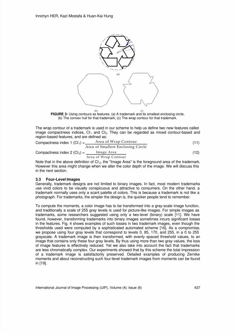
8/6/2019 International Journal of Image Processing (IJIP) Volume 4 Issue 6
http://slidepdf.com/reader/full/international-journal-of-image-processing-ijip-volume-4-issue-6 128/172
Innchyn HER, Kazi Mostafa & Huan-Kai Hung
International Journal of Image Processing (IJIP), Volume (4): Issue (6) 637
FIGURE 3: Using contours as features. (a) A trademark and its smallest enclosing circle,(b) The convex hull for that trademark, (c) The wrap contour for that trademark.
The wrap contour of a trademark is used in our scheme to help us define two new features calledimage compactness indices, CI 1 and CI 2. They can be regarded as mixed contour-based andregion-based features, and are defined as:Compactness index 1 (CI 1) = Area of Wrap Contour
Area of Smallest Enclosing Circle(11)
Compactness index 2 (CI 2) = Image AreaArea of Wrap Contour
(12)
Note that in the above definition of CI 2, the "Image Area" is the foreground area of the trademark.However this area might change when we alter the color depth of the image. We will discuss thisin the next section.
3.3 Four-Level ImagesGenerally, trademark designs are not limited to binary images. In fact, most modern trademarksuse vivid colors to be visually conspicuous and attractive to consumers. On the other hand, atrademark normally uses only a scant palette of colors. This is because a trademark is not like aphotograph. For trademarks, the simpler the design is, the quicker people tend to remember.
To compute the moments, a color image has to be transformed into a gray-scale image function,and traditionally a scale of 255 gray levels is used for picture-like images. For simple images astrademarks, some researchers suggested using only a two-level (binary) scale [11]. We havefound, however, transforming trademarks into binary images sometimes incurs significant lossesin the features. Fig. 4 shows examples of such losses in two trademark images, even though thethresholds used were computed by a sophisticated automated scheme [16]. As a compromise,
we propose using four gray levels that correspond to levels 0, 85, 170, and 255, in a 0 to 255grayscale. A trademark image is then transformed, with evenly spaced threshold values, to animage that contains only these four gray levels. By thus using more than two gray values, the lossof image features is effectively reduced. Yet we also take into account the fact that trademarksare less chromatically complex. Our experiments showed that by this scheme the total impressionof a trademark image is satisfactorily preserved. Detailed examples of producing Zernikemoments and about reconstructing such four-level trademark images from moments can be foundin [19].

8/6/2019 International Journal of Image Processing (IJIP) Volume 4 Issue 6
http://slidepdf.com/reader/full/international-journal-of-image-processing-ijip-volume-4-issue-6 129/172
Innchyn HER, Kazi Mostafa & Huan-Kai Hung
International Journal of Image Processing (IJIP), Volume (4): Issue (6) 638
FIGURE 4: Losing boundaries from using too few gray levels. (a) Some internal boundaries are missing,(b) The plus sign is gone.
3.4 Exclusive Trademark FeaturesThe feature values of an image are collectively used to identify the image. Thus, these featuresmust be appropriately extracted. For trademarks, there are additional yet unique concerns. First,a trademark can be registered with a principal pattern and that pattern plus a variety of frames,e.g., circular, square, or polygonal shapes. Framed versions are regarded as the same as theoriginal in trademark evaluation. Second, a chromatically altered image of a trademark pattern isalso considered equivalent to the original one. For example, a dark-colored trademark on a lightbackground is the same as the inversed, light trademark pattern on a dark background.
In this paper we highlight the quest of emulating the real trademark evaluation process. Hence, inextracting the features of one trademark we may need to consider not only the original design,but also its inversed image, and its core image. The core image refers to the central portion of theoriginal trademark that lies within a smaller concentric circle whose radius is 2/3 of the enclosingcircle. This core image is used to exclude the trademark frame and thus reduce the chances ofmisinterpretation. It is also noted that in real trademark retrieval the most important task is todetect confusingly similar designs, rather than to recover exactly like ones. Care has been takenin using features, so as to make our retrieval system neither under-restraining nor over-
restraining. In this paper, we use Zernike moments of orders 0 to 19 as main region-basedfeatures for trademarks. The lower-order (0 to 12) moments represent the rough content of thetrademark, whereas the higher-order moments delineate the minutia in the trademark image.
3.5 Weighting and NormalizationAccording to the trademark law, the degree of similarity between trademarks is the seriousness ofconfusion they cause for consumers. Obviously, this is a subjective judgment, and which mayvary among different designs. Thus, we employ for our hybrid system a human-machine interfacethat allows users to feedback and to adjust the weighting of any feature type. Weighting means toprescribe significance for each feature group, which is among, say, m distinct image featurecategories.
Combining the values from different feature categories requires a work called normalization. This
process is to ensure that all image features possess influences of similar order. Now let P be aninput trademark image, to be compared with the trademark database, which comprises n imageentries Q i, i=1 to n. Regarding the j th feature category, which contains k values, the similaritybetween images P and Q i is then defined as a Euclidean distance on the coordinate hyperspace[21], given by
( ) ( )1/2k 2 j j j j
i s s is 1
dist P , Q p q=
= −
∑ (13)

8/6/2019 International Journal of Image Processing (IJIP) Volume 4 Issue 6
http://slidepdf.com/reader/full/international-journal-of-image-processing-ijip-volume-4-issue-6 130/172
Innchyn HER, Kazi Mostafa & Huan-Kai Hung
International Journal of Image Processing (IJIP), Volume (4): Issue (6) 639
where js p and j
s iq are corresponding feature values of P and Q i. Now for the j th featurecategory, we scan through the entire database for the two extreme values:
( ) ( )
j j jii n
j j jii n
Min min dist P ,Q
Max max dist P ,Q≤
≤
=
= (14)
The normalized Euclidean distance, meaning the normalized similarity between images P and Q i regarding the j th feature category, is then
( ) ( ) j j ji j j
i j j
dist P ,Q MinDist P ,Q
Max Min
−=
− (15)
Adding the consideration of the weighting factor jw for the j th of a total of m feature categories,the gross similarity between images P and Q i is then:
( ) ( )=
= ⋅∑m
j j jG i i
j 1S P,Q w Dist P ,Q (16)
4. EXPERIMENTS & RESULTS
In this paper, 2020 trademark images were collected from various sources and compiled to formthe experimental database. These images had been of different sizes, colors, and complexity. Tobegin with, since we wanted to emphasize human perspectives, we recruited ten adult volunteers,aged from 20 to 30, three among them female, and asked them to pick from the sample databasesome groups of similar images visible to their naked eyes. Listed in Table 1 are the five groups ofsimilar trademarks hand-picked by the volunteers. These human culled images were to be usedas benchmarks as we tested our hybrid scheme.
Table 1: Human-Picked Groups of Similar Trademark Patterns
Note that each group in Table 1 actually stands for a certain aspect of trademark identification.The images in the first group, "Nike," all contain an abstract notion of a checkmark. In the secondgroup, "Goblet," either the snake or the goblet can deform its shape or change its color. The thirdgroup, "Recycle," is an example of inversed and framed trademark images. The fourth groupinvolves various postures of the "Michelin" Man. These figures are line drawings containing nosolid areas. The last group is "Monogram." Monograms are commonly used as trademarks inwestern countries and are also common victims of infringements.
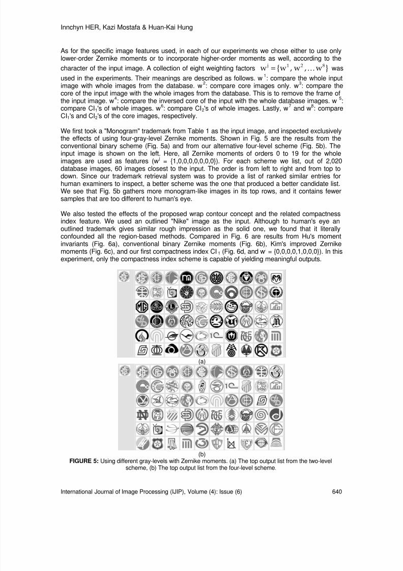
8/6/2019 International Journal of Image Processing (IJIP) Volume 4 Issue 6
http://slidepdf.com/reader/full/international-journal-of-image-processing-ijip-volume-4-issue-6 131/172
Innchyn HER, Kazi Mostafa & Huan-Kai Hung
International Journal of Image Processing (IJIP), Volume (4): Issue (6) 640
As for the specific image features used, in each of our experiments we chose either to use onlylower-order Zernike moments or to incorporate higher-order moments as well, according to thecharacter of the input image. A collection of eight weighting factors j 1 2 8w w , w , w = K wasused in the experiments. Their meanings are described as follows. w 1: compare the whole inputimage with whole images from the database. w 2: compare core images only. w 3: compare thecore of the input image with the whole images from the database. This is to remove the frame ofthe input image. w 4: compare the inversed core of the input with the whole database images. w 5:compare CI 1 's of whole images. w 6: compare CI 2's of whole images. Lastly, w 7 and w 8: compareCI1 's and CI 2's of the core images, respectively.
We first took a "Monogram" trademark from Table 1 as the input image, and inspected exclusivelythe effects of using four-gray-level Zernike moments. Shown in Fig. 5 are the results from theconventional binary scheme (Fig. 5a) and from our alternative four-level scheme (Fig. 5b). Theinput image is shown on the left. Here, all Zernike moments of orders 0 to 19 for the wholeimages are used as features (w j = 1,0,0,0,0,0,0,0). For each scheme we list, out of 2,020database images, 60 images closest to the input. The order is from left to right and from top todown. Since our trademark retrieval system was to provide a list of ranked similar entries forhuman examiners to inspect, a better scheme was the one that produced a better candidate list.We see that Fig. 5b gathers more monogram-like images in its top rows, and it contains fewer
samples that are too different to human's eye.
We also tested the effects of the proposed wrap contour concept and the related compactnessindex feature. We used an outlined "Nike" image as the input. Although to human's eye anoutlined trademark gives similar rough impression as the solid one, we found that it literallyconfounded all the region-based methods. Compared in Fig. 6 are results from Hu's momentinvariants (Fig. 6a), conventional binary Zernike moments (Fig. 6b), Kim's improved Zernikemoments (Fig. 6c), and our first compactness index CI 1 (Fig. 6d, and w j = 0,0,0,0,1,0,0,0). In thisexperiment, only the compactness index scheme is capable of yielding meaningful outputs.
(a)
(b)FIGURE 5: Using different gray-levels with Zernike moments. (a) The top output list from the two-level
scheme, (b) The top output list from the four-level scheme.
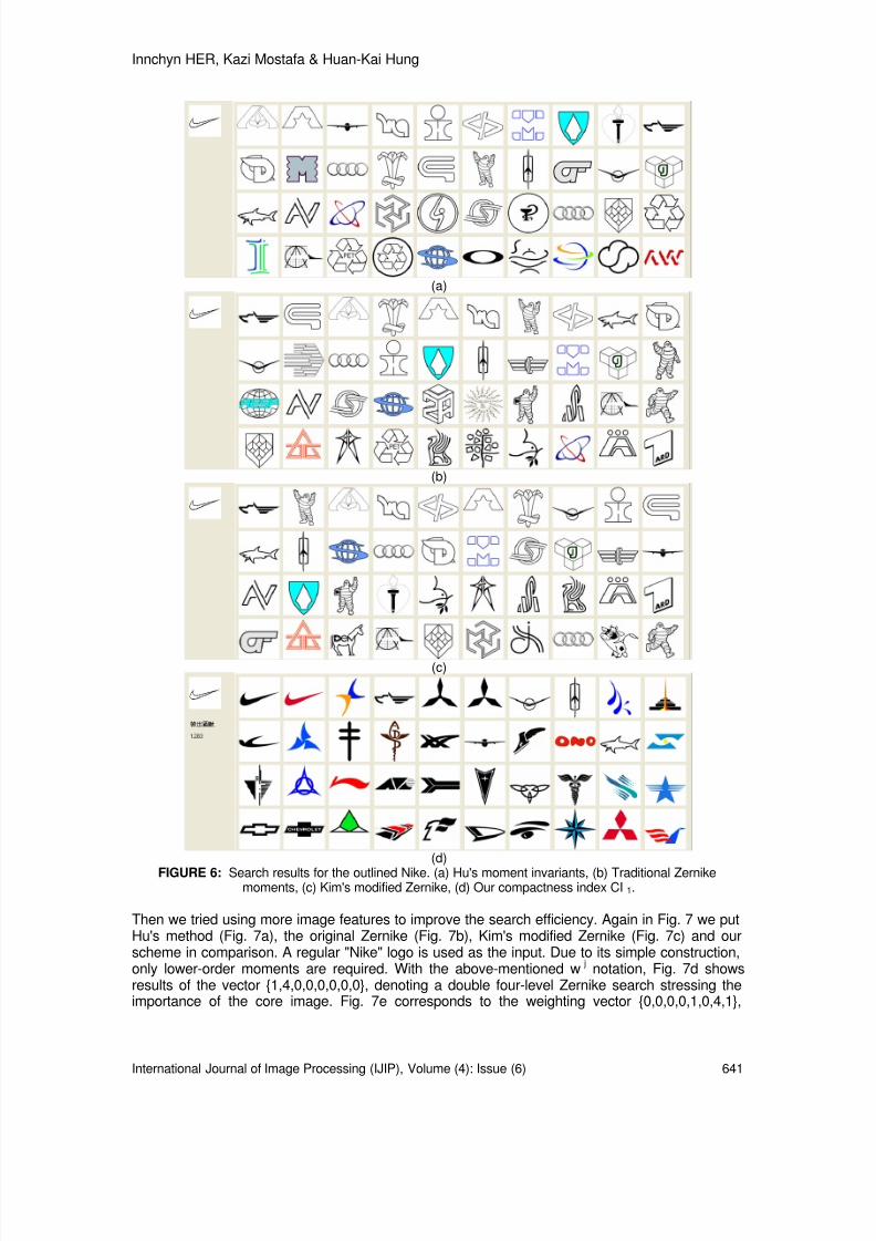
8/6/2019 International Journal of Image Processing (IJIP) Volume 4 Issue 6
http://slidepdf.com/reader/full/international-journal-of-image-processing-ijip-volume-4-issue-6 132/172
Innchyn HER, Kazi Mostafa & Huan-Kai Hung
International Journal of Image Processing (IJIP), Volume (4): Issue (6) 641
(a)
(b)
(c)
(d)FIGURE 6: Search results for the outlined Nike. (a) Hu's moment invariants, (b) Traditional Zernike
moments, (c) Kim's modified Zernike, (d) Our compactness index CI 1.
Then we tried using more image features to improve the search efficiency. Again in Fig. 7 we putHu's method (Fig. 7a), the original Zernike (Fig. 7b), Kim's modified Zernike (Fig. 7c) and ourscheme in comparison. A regular "Nike" logo is used as the input. Due to its simple construction,only lower-order moments are required. With the above-mentioned w j notation, Fig. 7d showsresults of the vector 1,4,0,0,0,0,0,0, denoting a double four-level Zernike search stressing theimportance of the core image. Fig. 7e corresponds to the weighting vector 0,0,0,0,1,0,4,1,

8/6/2019 International Journal of Image Processing (IJIP) Volume 4 Issue 6
http://slidepdf.com/reader/full/international-journal-of-image-processing-ijip-volume-4-issue-6 133/172
Innchyn HER, Kazi Mostafa & Huan-Kai Hung
International Journal of Image Processing (IJIP), Volume (4): Issue (6) 642
showing the effects of combining the two compactness indices, also emphasizing the core. Theweightings of Fig. 7f are 1,4,0,0,1,0,4,1, equivalent to the sum of the weightings of Fig. 7d andFig. 7e. From these figures we see that while Fig. 7d already produces a better listing than Figs.7a to 7c, Fig. 7f produces the best result of all. All but one trademark in the "Nike" group in Table1 are listed in the top 20 (top 1%, out of 2,020) candidates of Fig. 7f.
Similar satisfactory results of the proposed scheme were obtained for a monogram trademark.Again, Figs. 8a to 8c are results from the three existing schemes, and Figs. 8d to 8f are resultsfrom three variations of the proposed scheme. The weighting vectors for Figs. 8d to 8f are5,5,0,0,0,0,0,0, 0,0,0,0,10,1,0,0, and 5,5,0,0,10,1,0,0, respectively. For monogram imageswe do not need to emphasize the core. Note that different image type may require differentweighting factor assortments. In the previous two examples we have not used w 3 and w 4. Theyare by no means less useful. Many additional examples involving framed or inversed trademarksor even various kinds of noise can be found in [16].
(a)
(b)
(c)FIGURE 7: Comparison between schemes. (a) Hu's moment invariants, (b) The original Zernike, (c) Kim's
modified Zernike, (d) Our double four-level Zernike, (e) Our Compactness indices,(f) Combining double Zernike and Compactness indices.
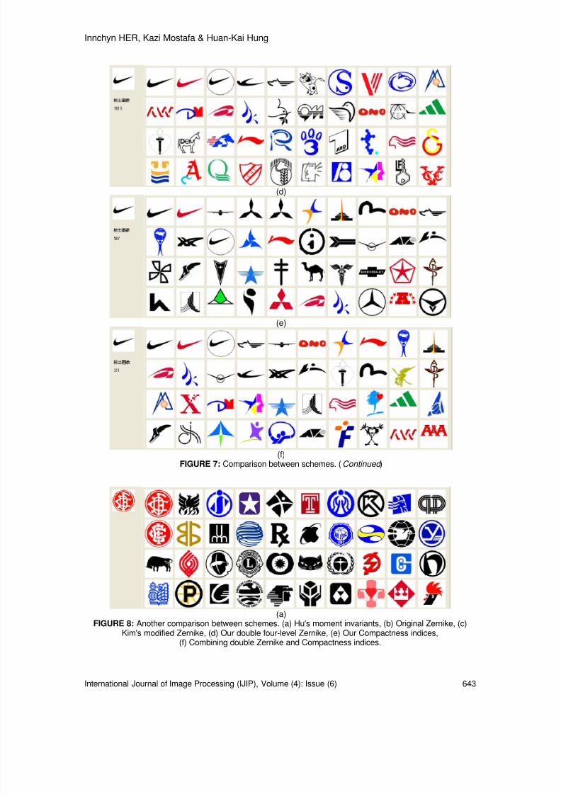
8/6/2019 International Journal of Image Processing (IJIP) Volume 4 Issue 6
http://slidepdf.com/reader/full/international-journal-of-image-processing-ijip-volume-4-issue-6 134/172
Innchyn HER, Kazi Mostafa & Huan-Kai Hung
International Journal of Image Processing (IJIP), Volume (4): Issue (6) 643
(d)
(e)
(f)FIGURE 7: Comparison between schemes. ( Continued )
(a)FIGURE 8: Another comparison between schemes. (a) Hu's moment invariants, (b) Original Zernike, (c)
Kim's modified Zernike, (d) Our double four-level Zernike, (e) Our Compactness indices,(f) Combining double Zernike and Compactness indices.
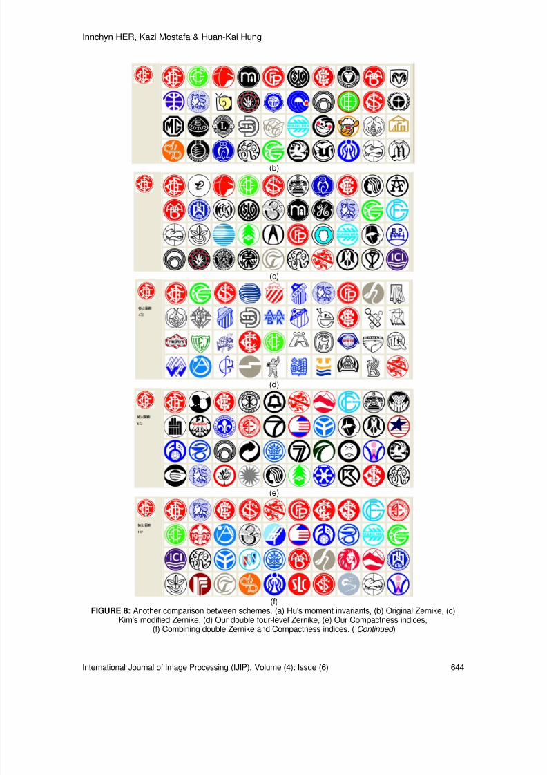
8/6/2019 International Journal of Image Processing (IJIP) Volume 4 Issue 6
http://slidepdf.com/reader/full/international-journal-of-image-processing-ijip-volume-4-issue-6 135/172
Innchyn HER, Kazi Mostafa & Huan-Kai Hung
International Journal of Image Processing (IJIP), Volume (4): Issue (6) 644
(b)
(c)
(d)
(e)
(f) FIGURE 8: Another comparison between schemes. (a) Hu's moment invariants, (b) Original Zernike, (c)
Kim's modified Zernike, (d) Our double four-level Zernike, (e) Our Compactness indices,(f) Combining double Zernike and Compactness indices. ( Continued )

8/6/2019 International Journal of Image Processing (IJIP) Volume 4 Issue 6
http://slidepdf.com/reader/full/international-journal-of-image-processing-ijip-volume-4-issue-6 136/172
Innchyn HER, Kazi Mostafa & Huan-Kai Hung
International Journal of Image Processing (IJIP), Volume (4): Issue (6) 645
On the whole, for the five groups of trademark images in Table 1, the performance of our methodis summarized as follows. In average, both our double Zernike schemes (as Figs. 7d and 8d) andCI-only schemes (as Fig. 7e and 8e) got roughly 60% of human-picked images in their top 40 (top2%) image listings. This was no better than Kim's modified Zernike (65% in average) and more orless equivalent to traditional Zernike (58% in average). But it is noted that since our double-Zernike and CI's are very different image features, the combination of the two (as Figs. 7f and 8f)yielded very good (95% in average) results. But with what kind of trademark did we show greatestadvantage? We will say in dealing with the "Goblet" images, our method outperformed hugelyother methods (100% vs. 25%). The next were the "Monogram" and the "Nike" trademarks. Forthe "Recycle" and the "Michelin" groups, only small improvement was achieved. This wasbecause both traditional Zernike or Kim's modified Zernike already treated them quite well. Hybridsystem may not be able to retrieve distributed shape or image like shape. Because we wereconcentrated only trademark retrieval and this kind of shape is not familiar as a trademark.However, our method was still a competitive choice because we could deal with outlined, framed,and inversed variation of the trademarks.
In all above experiments, a 64×64 image size was used for the input and for all the databaseimages. An input image must go through a series of preprocessing processes such as conversionto four gray-level, obtaining the smallest enclosing circle, and proper geometric transformation. Allimage features are then extracted, paired with their weighting factors and compared with storeddata in the database. The whole process for a 200×200 input image takes about 8.5 seconds onan Intel Celeron 2.66 GHz computer with 512 Mb RAM. Lastly, we think it is interesting to mentionthat when we doubled the resolution of all images (input and database) to 128×128, only slightchange was observed in the results.
5. CONCLUSIONS
We have presented in this paper the framework of a hybrid trademark retrieval system. Surveysof human responses to different trademark aspects were conducted and the results were used asbenchmarks for the system. The task of the computer was only to provide, according to thebenchmarks, a good ranked list of similar candidates. Both region-based image features (i.e.,four-gray-level Zernike moments) and contour-base features (the proposed compactness indices)were used. A simplified method for finding the smallest enclosing circle was also presented.Features of different categories were conjoined via a weighting scheme particularly useful fordealing with framed or inversed trademark variations. Experiments have verified that, whenhuman viewpoints obtained from consumer surveys were used as standards, this hybrid schemeperformed considerably better than some existing retrieval methods.
6. ACKNOWLEDGEMENTSThe authors are greatly indebted to Director Jiou-Ru Chang of Taiwan Intellectual Property Office(Kaohsiung Branch) for his kind assistance and precious comments offered to this research.
7. REFERENCES[1] United States Patent and Trademark Office, "2007 Design Code Updates", USPTO Design
Search Code Manual , http://tess2.uspto.gov/tmdb/dscm/dsc_ap.htm, accessed 2010
[2] H. Freeman, " On the Encoding of Arbitrary Geometric Configurations ". IRE Trans. ElectronicComputing, 10: 260-268, 1961
[3] H. L. Peng and S. Y. Chen, " Trademark Shape Recognition Using Closed Contours ". PatternRecognition Letters, 18: 791-803, 1997
[4] C. C. Huang and I. Her, " Homomorphic Graph Matching of Articulated Objects by An Integrated Recognition Scheme ". Expert Systems with Applications, 31: 116-129, 2006
8/6/2019 International Journal of Image Processing (IJIP) Volume 4 Issue 6
http://slidepdf.com/reader/full/international-journal-of-image-processing-ijip-volume-4-issue-6 137/172
Innchyn HER, Kazi Mostafa & Huan-Kai Hung
International Journal of Image Processing (IJIP), Volume (4): Issue (6) 646
[5] P. Y. Yin and C. C. Yeh, " Content-based Retrieval from Trademark Databases ". PatternRecognition Letters, 23: 113-126, 2002
[6] M. K. Hu, " Visual Pattern Recognition by Moment Invariants ". IRE Trans. Information Theory,pp. 179-187, 1962
[7] J. L. Shih and L. H. Chen, " A New System for Trademark Segmentation and Retrieval ".Image and Vision Computing, 19: 1011-1018, 2001.
[8] G. Ciocca and R. Schettini, " Content-based Similarity Retrieval of Trademarks Using Relevance Feedback ". Pattern Recognition, 34: 1639-1655, 2001
[9] Y. S. Kim and W. Y. Kim, " Content-based Trademark Retrieval System Using a Visually Salient Feature ". Image and Vision Computing, 16: 931-939, 1998
[10] H. K. Kim, J. D. Kim, D. G. Sim and D. I. Oh, " A Modified Zernike Moment Shape Descriptor Invariant to Translation, Rotation and Scale for Similarity-based Image Retrieval ". IEEEInternational Conference on Multimedia and Expo, 1: 307-310, 2000
[11] N. K. Kamila, S. Mahapatra and S. Nanda, " Invariance Image Analysis Using Modified Zernike Moments ". Pattern Recognition Letters, 26: 747-753, 2005
[12] United States Patent and Trademark Office, Trademark Manual of Examining Procedure (TMEP) , 5 th ed., USPTO, 2007
[13] United States Patent and Trademark Office, U.S. Trademark Law , USPTO, 2010
[14] Taiwan Intellectual Property Office, Taiwan Trademark Law , TIPO, 2003
[15] J. R. Chang, Director, Taiwan Intellectual Property Office, Kaohsiung Branch, Interview byauthor, 2006
[16] H. K. Hung, " A Computer-assisted Trademark Retrieval System with Zernike Moment and
Image Compactness Indices ". Master thesis, Electro-Mechanical Engineering Department,National Sun Yat-sen University, Taiwan, 2006
[17] S. D. Lin, S. C. Shie, W. S. Chen, B. Y. Shu, X. L. Yang and Y. L. Su, " Trademark Image Retrieval by Distance-Angle Pair-wise Histogram ". International J. Imaging Systems andTechnology, 15: 103-113, 2005
[18] M. Teague, " Image Analysis via the General Theory of Moments ". J. Optical Society ofAmerica, 70: 920-930, 1980
[19] M. de Berg, M. van Kreveld, M. Overmars and O. Schwarzkopf, Computational Geometry: Algorithms and Applications , New York : Springer, (2000)
[20] I. Her, " Geometric Transformations on the Hexagonal Grid ". IEEE Trans. Image Processing,4: 1213-1222, 1995
[21] I. Her, " A Symmetrical Coordinate Frame on the Hexagonal Grid for Computer Graphics and Vision ". ASME J. Mechanical Design, 115: 447-449, 1993.
[22] J. Schietse, J. Eakins & R. Veltkamp, “ Practice and Challenges in Trademark Image Retrieval ”. ACM International Conference on Image and Video Retrieval, Amsterdam, TheNetherlands, 2007

8/6/2019 International Journal of Image Processing (IJIP) Volume 4 Issue 6
http://slidepdf.com/reader/full/international-journal-of-image-processing-ijip-volume-4-issue-6 138/172
Thiyagarajan, Arulselvi & Sainarayanan
International Journal of Image Processing (IJIP), Volume (4): Issue (6) 647
Statistical Models for Face Recognition System WithDifferent Distance Measures
R.Thiyagarajan [email protected] of Electronics and
Instrumentation Engineering Annamalai University Annamalai Nagar, India
S.Arulselvi [email protected] of Electronics and Instrumentation Engineering Annamalai University Annamalai Nagar, India
G.Sainarayanan [email protected] R&D ICTACT, Chennai India
Abstract
Face recognition is one of the challenging applications of image processing.Robust face recognition algorithm should posses the ability to recognize identitydespite many variations in pose, lighting and appearance. Principle ComponentAnalysis (PCA) method has a wide application in the field of image processing fordimension reduction of the data. But these algorithms have certain limitations likepoor discriminatory power and ability to handle large computational load. Thispaper proposes a face recognition techniques based on PCA with Gaborwavelets in the preprocessing stage and statistical modeling methods like LDAand ICA for feature extraction. The classification for the proposed system is doneusing various distance measure methods like Euclidean Distance(ED), CosineDistance (CD), Mahalanobis Distance (MHD) methods and the recognition ratewere compared for different distance measures. The proposed method has beensuccessfully tested on ORL face data base with 400 frontal imagescorresponding to 40 different subjects which are acquired under variableillumination and facial expressions. It is observed from the results that use ofPCA with Gabor filters and features extracted through ICA method gives arecognition rate of about 98% when classified using Mahalanobis distanceclassifier. This recognition rate stands better than the conventional PCA and PCA+ LDA methods employing other and classifier techniques.
Keywords: Face Recognition, Statistical Models, Distance measure methods, PCA/LDA/ICA.
1. INTRODUCTION
Human face detection and recognition is an active area of research spanning several disciplinessuch as image processing, pattern recognition and computer vision with wide range ofapplications such as personal identity verification, video-surveillance, facial expression extraction,

8/6/2019 International Journal of Image Processing (IJIP) Volume 4 Issue 6
http://slidepdf.com/reader/full/international-journal-of-image-processing-ijip-volume-4-issue-6 139/172

8/6/2019 International Journal of Image Processing (IJIP) Volume 4 Issue 6
http://slidepdf.com/reader/full/international-journal-of-image-processing-ijip-volume-4-issue-6 140/172
Thiyagarajan, Arulselvi & Sainarayanan
International Journal of Image Processing (IJIP), Volume (4): Issue (6) 649
In this proposed work, the gabor wavelets are used in the pre processing stage. This gaborfiltered face images results in a large gabor feature vector. This larger dataset is reduced to asmaller dimension using the PCA algorithm which extracts the principle features (top eigenvectors). The reduced dataset is further processed using the two feature extraction techniquesnamely LDA and ICA. This results in the most discriminating and the most independent featuresof the input data respectively. The classification is done using the minimum distance measuremethods like ED, CD and MD methods. The results are compared and tabulated for the resultedrecognition rate. In comparison with the conventional use of PCA and LDA alone, the proposedmethod gives a better recognition rate. The algorithm is tested with the use of ORL face databasewith 200 training and 200 test samples. The feasibility of the new algorithm has beendemonstrated by experimental results. Encouraging results were obtained for the proposedmethod compared to conventional methods.
This paper is organized as follows: Section 2 deals with the basics of Gabor wavelets and Gaborfeatures. Section 3 deals background of PCA and Eigenfaces. Section 4 deals with LDA. Section5 details about ICA. Section 6 deals with the various types of distance measure method. Theproposed method is reported in section 7. Experimental results are presented in Section 9 andfinally, Section 10 gives the conclusions.
2. GABOR WAVELETThe prime motive behind the feature based approach is the representation of face image in a verycompact manner, thus reducing the memory used. Such methods gains importance as the size ofthe database is increased. This feature based method in a face recognition system aims to findthe important local features on a face and represent the corresponding features in an efficientway. The selection of feature points and representation of those values has been a difficult taskfor a face recognition system. Physiological studies found that simple cells present in humanvisual cortex can be selectively tuned to orientation as well as spatial frequency. J.G.Daugman[7]has worked on this and confirmed that the response of the simple cell could be approximated by2D Gabor filters.
Because of their biological relevance and computational properties, Gabor wavelets wereintroduced into the area of image processing [8,9]. The Gabor wavelets, whose kernels are
similar to the 2D receptive field profiles of the mammalian cortical simple cells, exhibit desirablecharacteristics of spatial locality and orientation selectivity, and are optimally localized in thespace and frequency domains. These drawbacks were overcome by Gabor wavelets. The Gaborwavelet is well known for its effectiveness to extract the local features in an image. It has theability to exhibit the desirable characteristics of capturing salient visual properties such as spatiallocalization, orientation selectivity, and spatial frequency selectivity. This method is robust tochanges in facial expression, illumination and poses. Applying statistical modeling methods likePCA, LDA, ICA for the Gabor filtered feature vector, results in a crisp gabor feature vectors. Inorder to consider all the gabor kernels, all the features were concatenated to form a single gaborfeature vector. This high dimensional gabor vector space is then reduced using the PCA. Furtheron applying the ICA and LDA on the reduced data, the more independent and discriminatingfeatures were obtained.
The Gabor wavelets (kernels, filters) can be defined as follows [7], [8]:
( ) ( )
−−
−=Ψ
2
2expexp
2exp ,2
22
,2
,,σ
σ µ
µ
µ ν µ zik zk
k z vv
v (1)
Where µ and v in Eqn. 1 define the orientation and scale of the Gabor kernels, z = (x,y) and ||.||denotes the norm operator, and the wave vector k µ,v is defined as follows:
) µ ν ν µ Φ= ik k exp, (2)

8/6/2019 International Journal of Image Processing (IJIP) Volume 4 Issue 6
http://slidepdf.com/reader/full/international-journal-of-image-processing-ijip-volume-4-issue-6 141/172
Thiyagarajan, Arulselvi & Sainarayanan
International Journal of Image Processing (IJIP), Volume (4): Issue (6) 650
where k v = k max /fv and φ µ = πµ /8, k max is the maximum frequency, and f is the spacing factorbetween kernels in the frequency domain [9]. The Gabor kernels in Eq. 1 are all self-similar sincethey can be generated from one filter, the mother wavelet, by scaling and rotation via the wavevector k µ,v. Each kernel is a product of a gaussian envelope and a complex plane wave, whilethe first term in Eq. 2 determines the oscillatory part of the kernel and the second termcompensates for the DC value. The effect of the DC term becomes negligible when theparameter σ , which determines the ratio of the gaussian window width to wavelength, hassufficiently large values. In most cases the use of gabor wavelets of five different scales, v ∈ 0,….., 4 and eight orientations, µ ∈ 0,…..,7is used for representational bases. Fig. 2 showsthe Gabor kernels at five scales and eight orientations, with the following parameters: σ = 2 π ,kmax = π /2 and f = .
2.1 Gabor Wavelet RepresentationThe Gabor wavelet representation of an image is the convolution of the image with a family ofGabor kernels as defined by Eq. 3. Let I(x,y) be the gray level distribution of an image, theconvolution of image I and a Gabor kernel ψµ,v is defined as follows.
( ) ( ) ( ) z z I zO ν µ ν µ ,, * Ψ=(3)
where z = (x,y) and * denotes the convolution operator, and O µ,v (z) is the convolution resultcorresponding to the gabor kernel at orientation µ and scale v. Therefore, the set S = O µ,v (z) , forµ ∈ 0,…..7 and v ∈ 0,…..4 forms the gabor wavelet representation of the image I(z).Applying the convolution theorem, we can derive each O µ,v (z) from Eq. 3 via the Fast FourierTransform (FFT):
₣ Oµ,v (z) = ₣I(z)₣ ψ µ,v(z) (4)Oµ,v (z) = ₣ -1 ₣ I(z)₣ ψµ,v(z) (5)
where ₣ and ₣ -1 denote the Fourier and inverse Fourier transform, respectively. Fig.2 and 3 showthe Gabor wavelet representation (the real part of gabor kernels with five scales and eightorientations and the magnitude of gabor kernels at five different scales). The input frontal faceimage as shown in Fig 4 is preprocessed using these kernels and the resultant convolution outputof the image and the kernels are as shown in Fig. 5 (Real part of the convolution output of asample image) and Fig. 6 (Magnitude of the convolution output of a sample image). Toencompass different spatial frequencies, spatial localities, and orientation selectivities into asingle augmented feature vector, concatenate all these gabor representations.
FIGURE 2. Gabor Kernels (Real part with five scales and eight orientations)

8/6/2019 International Journal of Image Processing (IJIP) Volume 4 Issue 6
http://slidepdf.com/reader/full/international-journal-of-image-processing-ijip-volume-4-issue-6 142/172
Thiyagarajan, Arulselvi & Sainarayanan
International Journal of Image Processing (IJIP), Volume (4): Issue (6) 651
FIGURE 3. Magnitude of Gabor Kernel at five different scales.
FIGURE 4. Sample frontal image
FIGURE 5 . Real part of the convolution output of the sample image
FIGURE 6. Magnitude of the convolution output of the sample image.

8/6/2019 International Journal of Image Processing (IJIP) Volume 4 Issue 6
http://slidepdf.com/reader/full/international-journal-of-image-processing-ijip-volume-4-issue-6 143/172
Thiyagarajan, Arulselvi & Sainarayanan
International Journal of Image Processing (IJIP), Volume (4): Issue (6) 652
Before the concatenation, each O µ,v(z) is down sampled by a factor ρ to reduce the spacedimension. Then constructing a vector out of the O µ,v(z) by concatenating its rows (or columns).Now, let O µ,v(ρ ) denote the vector constructed from O µ,v(z) (down sampled by ρ), the augmentedgabor feature vector X( ρ ) is then defined as follows:
X(ρ) = (O( ρ)t0,0 O(ρ)t0,1 ….. O( ρ)t4,7 ) (6)
where t is the transpose operator. The augmented gabor feature vector thus encompasses all theelements (down sampled ) of the gabor wavelet representation set, S = O µ,v (z) : µ ∈ 0,…..7 ,v ∈ 0,…..4 as important discriminating information. Fig. 6 shows (in image form rather than invector form) an example of the augmented Gabor feature vector, where the down sampling factoris 64, i.e. ρ = 64.
3. PRINCIPLE COMPONENT ANALYSISThe Principal Component Analysis (PCA) is a widely accepted and a successful technique thathas been used for image compression and image recognition .The purpose of this method is toreduce the large dimensionality of the data (observed variables) to a reduced dimensionality offeatures (independent variables), which describe the data economically with a strong correlationbetween data and features [2]. These characteristic features are called eigen faces in the face
recognition domain or principle components generally. In a face recognition system, PCA cantransform each original image of the training set into a corresponding eigenface. An importantfeature of PCA is that reconstruction of original image is possible by combining the all eigenfacesfrom the training set. These eigenfaces are nothing but characteristic features of the trainingfaces. Therefore summing up all the eigen faces in right proportion results in the original faceimage.
By using all the eigenfaces extracted from original images, exact reconstruction of the originalimages is possible. But for practical applications only certain part of the eigenfaces is used. Thenthe reconstructed image is an approximation of the original image. However losses due toomitting some of the eigenfaces can be minimized. This happens by choosing only the mostimportant features (eigenfaces)[2].
3.1 Mathematics of PCAA 2-D face image can be represented as 1-D vector by concatenating each row (or column) into a long thinvector.
1. Assume the training sets of images represented by Г1, Г2, Г3,…, Гm, with each image Г(x,y)where (x,y) is the size of the image represented by p and m is the number of training images.Converting each image into set of vectors given by (m x p).
2. The mean face Ψ is given by:
∑ =Γ =Ψ
m
i im 1
1
(7)3. The mean-subtracted face is given by( Φ i):
Ψ−Γ =Φii (8)
where i = 1, 2, 3….m. and A = [ Φ 1, Φ 2 … Φm,] is the mean-subtracted matrix with size Amp.4. By implementing the matrix transformations, the vector matrix is reduced by:T pmmpmm A AC ×=
(9)where C is the covariance matrix
5. Finding the eigen vectors V mm and eigen values λ m from the C matrix and ordering the eigenvectors by highest eigen values.
6. With the sorted eigen vector matrix, Φm is adjusted. These vectors determine the linearcombinations of the training set images to form the eigen faces represented by U k as follows

8/6/2019 International Journal of Image Processing (IJIP) Volume 4 Issue 6
http://slidepdf.com/reader/full/international-journal-of-image-processing-ijip-volume-4-issue-6 144/172
Thiyagarajan, Arulselvi & Sainarayanan
International Journal of Image Processing (IJIP), Volume (4): Issue (6) 653
∑ =Φ= m
n knnk V U 1 ,where , k = 1, 2…m. (10)
7. Instead of using m eigen faces, m ′ eigen faces (m ′<< m) is considered as the most significanteigen vectors provided for training of each individual.
8. With the reduced eigen face vector, each image has its face vector given by( )Ψ−Γ = T
k k U W , k = 1, 2… m
′. (11)9. The weights form a feature vector given by
[ ]'21 ,..., mT www=Ω
(12)10. These feature vectors are taken as the representational basis for the face images with
reduced dimension.11. The reduced data is taken as the input to the next stage for extricating discriminating featureout of it.
4. LINEAR DISCRIMINANT ANALYSISThe goal of PCA on choosing a lower dimensional basis is to minimize the reconstruction error.This is not the major concern in pattern recognition applications, whose goal is to maximize therecognition rate. The Linear Discriminant Analysis (LDA) provides a procedure to determine a set
of axes whose projections of different groups have the maximum separation. The LDA searchesfor those vectors in the underlying space that best discriminates among classes (rather thanthose that best describe the data).
When the training data set are labeled for each identity, supervised training techniques like LDAare more profitable for feature extraction compared with methods of unsupervised learning. Byapplying the supervised learning, illumination variation and pose variation will be removed andretaining the identity information. The LDA provides a procedure to determine a set of axeswhose projections of different groups have the maximum separation. This procedure can bedescribed as follows.
Suppose that the sample consists of p face images from where m j images are of individual j, for j = 1... g.
Let µ be the mean feature vector of images from individuals j. The samples between individualcovariance matrix is defined as
S B = T (13)
SW = T (14)
Where µ i denotes the mean image of the class selected (individual) and µ denotes the meanimage of the entire data set, and p denotes the number of images in the entire data set.
The eigenvectors of LDA are called “fisherfaces”. LDA transformation is strongly dependent onthe number of classes (c), the number of samples (m), and the original space dimensionality (d).It is possible to show that there are almost (c-1) nonzero eigenvectors. (c-1) being the upperbound of the discriminant space dimensionality. For Sw to be a non singular matrix, it is requiredto have (d+c) samples in the training set [10]. It is impossible to guarantee this condition in manyreal applications. Consequently, an intermediate transformation is applied to reduce thedimensionality of the image space. To this end, PCA is used. Now LDA derives a low dimensionalrepresentation of a high dimensional face feature vector of PCA. From Eqn. 15, the covariancematrix C is obtained as follows
C = S W-1 * SB (15)

8/6/2019 International Journal of Image Processing (IJIP) Volume 4 Issue 6
http://slidepdf.com/reader/full/international-journal-of-image-processing-ijip-volume-4-issue-6 145/172

8/6/2019 International Journal of Image Processing (IJIP) Volume 4 Issue 6
http://slidepdf.com/reader/full/international-journal-of-image-processing-ijip-volume-4-issue-6 146/172
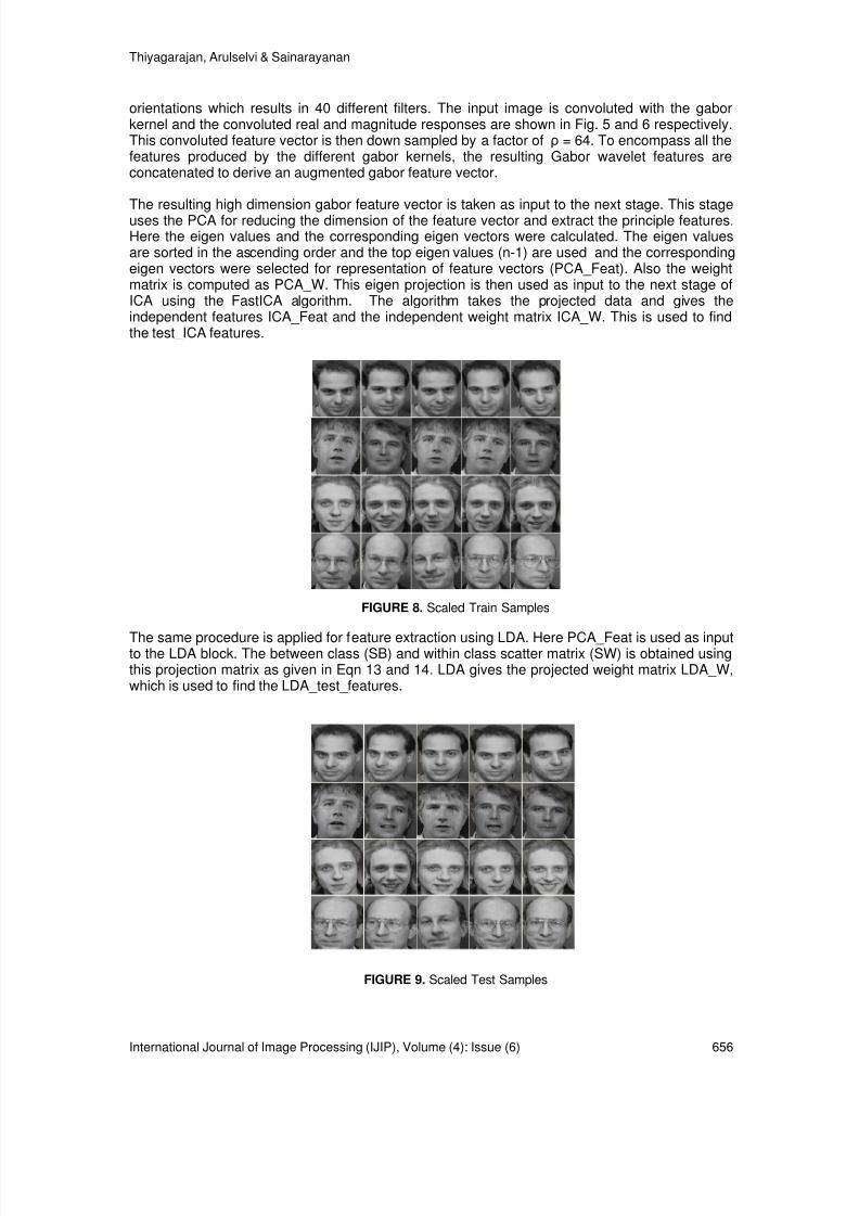
8/6/2019 International Journal of Image Processing (IJIP) Volume 4 Issue 6
http://slidepdf.com/reader/full/international-journal-of-image-processing-ijip-volume-4-issue-6 147/172
Thiyagarajan, Arulselvi & Sainarayanan
International Journal of Image Processing (IJIP), Volume (4): Issue (6) 656
orientations which results in 40 different filters. The input image is convoluted with the gaborkernel and the convoluted real and magnitude responses are shown in Fig. 5 and 6 respectively.This convoluted feature vector is then down sampled by a factor of ρ = 64. To encompass all thefeatures produced by the different gabor kernels, the resulting Gabor wavelet features areconcatenated to derive an augmented gabor feature vector.
The resulting high dimension gabor feature vector is taken as input to the next stage. This stageuses the PCA for reducing the dimension of the feature vector and extract the principle features.Here the eigen values and the corresponding eigen vectors were calculated. The eigen valuesare sorted in the ascending order and the top eigen values (n-1) are used and the correspondingeigen vectors were selected for representation of feature vectors (PCA_Feat). Also the weightmatrix is computed as PCA_W. This eigen projection is then used as input to the next stage ofICA using the FastICA algorithm. The algorithm takes the projected data and gives theindependent features ICA_Feat and the independent weight matrix ICA_W. This is used to findthe test_ICA features.
FIGURE 8. Scaled Train Samples
The same procedure is applied for feature extraction using LDA. Here PCA_Feat is used as inputto the LDA block. The between class (SB) and within class scatter matrix (SW) is obtained usingthis projection matrix as given in Eqn 13 and 14. LDA gives the projected weight matrix LDA_W,which is used to find the LDA_test_features.
FIGURE 9. Scaled Test Samples

8/6/2019 International Journal of Image Processing (IJIP) Volume 4 Issue 6
http://slidepdf.com/reader/full/international-journal-of-image-processing-ijip-volume-4-issue-6 148/172
Thiyagarajan, Arulselvi & Sainarayanan
International Journal of Image Processing (IJIP), Volume (4): Issue (6) 657
In the recognition stage, the test samples are preprocessed as done in the training stage. Withthe weight matrix from the PCA stage and the test image, the test features (PCA_Test_Feature)were obtained. This PCA_Test_Feature when convoluted with ICA_W gives the test features(ICA_test). The same procedure is used to obtain the test features for LDA method (LDA_testand LDA_W). The classification stage uses different distance measure methods. Here the trainingand test feature vectors are considered. For a given sample image, test feature vector is foundand the distance between this test feature vector and the all the training feature vectors arecalculated. From the distance measure, the index with minimum distance represents therecognized face from the training set.
8. RESULT AND DISCUSSION
The effectiveness of the proposed system is tested with ORL Face database and the results arecompared for the following experimental setups.
1. Gabor with PCA.2. Gabor with PCA and LDA.3. Gabor with PCA and ICA.
For each of the above said feature extraction method, the extracted features is used as it is,followed by classification using these three distance measures. The number of featuresconsidered for recognition is varied and the corresponding recognition rate is given in Table 1-3.The successfulness of the proposed method is compared with some popular face recognitionschemes like Gabor wavelet based classification [15], the PCA method [16], the LDA method[17], and ICA based systems[18].
S.No Distance Features40 50 66 100 200
1. Euclidean 87.0 89.3 93.2 93.7 94.02. Cosine 87.5 91.0 95.0 95.9 96..03. Mahalanobis 89.3 92.5 96.1 96.9 97.0
TABLE 1 : Features Vs Recognition rate for different distance measure methods(Gabor wavelets and PCA method for feature extraction)
S.No Distance Features40 50 66 100 200
1. Euclidean 87.8 90.1 94.3 95.2 95.32. Cosine 88.4 91.4 93.6 96.8 97.1
3. Mahalanobis 90.0 93.5 94.5 97.1 98.0TABLE 2 : Features Vs Recognition rate for different distance measure methods
(Gabor wavelets and PCA method for feature extraction)
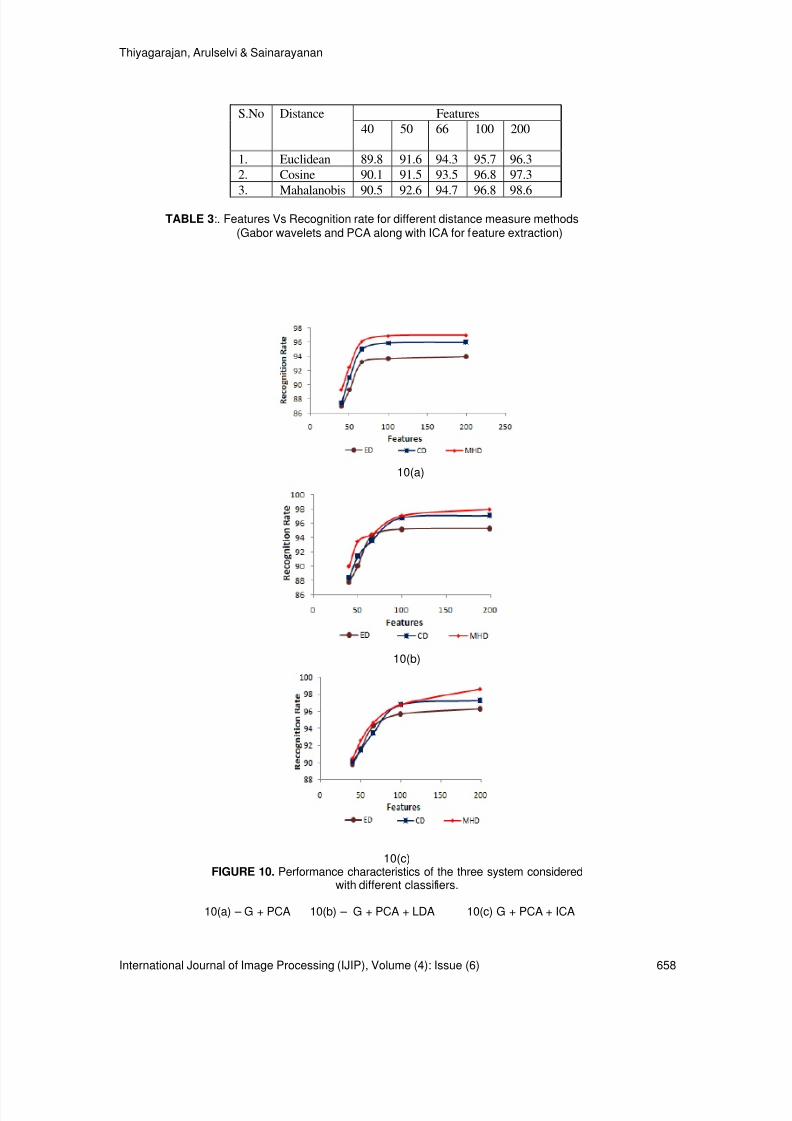
8/6/2019 International Journal of Image Processing (IJIP) Volume 4 Issue 6
http://slidepdf.com/reader/full/international-journal-of-image-processing-ijip-volume-4-issue-6 149/172
Thiyagarajan, Arulselvi & Sainarayanan
International Journal of Image Processing (IJIP), Volume (4): Issue (6) 658
S.No Distance Features40 50 66 100 200
1. Euclidean 89.8 91.6 94.3 95.7 96.32. Cosine 90.1 91.5 93.5 96.8 97.3
3. Mahalanobis 90.5 92.6 94.7 96.8 98.6TABLE 3 :. Features Vs Recognition rate for different distance measure methods
(Gabor wavelets and PCA along with ICA for feature extraction)
10(a)
10(b)
10(c)FIGURE 10. Performance characteristics of the three system considered
with different classifiers.
10(a) – G + PCA 10(b) – G + PCA + LDA 10(c) G + PCA + ICA

8/6/2019 International Journal of Image Processing (IJIP) Volume 4 Issue 6
http://slidepdf.com/reader/full/international-journal-of-image-processing-ijip-volume-4-issue-6 150/172
Thiyagarajan, Arulselvi & Sainarayanan
International Journal of Image Processing (IJIP), Volume (4): Issue (6) 659
FIGURE 11. Performance characteristics of the proposed system with othermethods using Mahalanobis Distance Classifier
9. CONCLUSIONIn this proposed work, a Gabor feature based method is introduced for face recognition system.For different scales and orientations of the Gabor filter, the input image is filtered. Using PCA, thehigh dimensionality of the Gabor feature vector is reduced followed by feature extraction usingICA and LDA. Three different types of distance measure methods namely Euclidean Distance,Cosine Distance, and Mahalanobis Distance are used for classification. From the simulationresults, it has been found that the recognition rate for the selected database is high with featuresextracted from Gabor filters based on ICA than with LDA and simple PCA methods. Thisrecognition rate is obtained by varying the number of features at the PCA stage. The results aretabulated in the Table .1 to 3. For all these three systems, the number of PCA features assumedfor further processing is 40, 50, 66, 100, and 199.
From the results, it is obvious that as the number of features selected in PCA increase, then themore discriminating features is obtained from the LDA method and the more independentfeatures is obtained from the ICA method. This helps to increase the recognition rate percentagefor the proposed system. But this in turn increases the computational load. Also from the results,when compared to other classifiers tested in the proposed system, Mahalanobis distanceclassifier does a better classification for the Gabor features based on ICA method.
10. REFERENCES1. W. Zaho, R.Chellappa, P.J.Philips and A.Rosenfeld, “Face recognition A literature survey,” ACM
Computing Surveys, 35(4):399– 458,2003.
2. M. Kirby and L. Sirovich, “Application of the karhunenloeve procedure for the characterization of humanfaces”, IEEE Trans. Pattern Analysis and Machine Intelligence, 12 (1):103-108,1990.
3. M. Turk and A. Pentland, “ Eigenfaces for recognition ” J. Cognitive Neuroscience, 3: 71-86,1991.
4. D. L. Swets and J. J. Weng, “ Using discriminant eigenfeatures for image retrieval ”, IEEE Trans. PAMI.,18(8):831-836,1996.
5. P. Belhumeur J. P. Hespanha and D. J. Kriegman, “ Eigenfaces vs. Fisherfaces; Recognition using class specific linear projection ”, Pattern Recognition and Machine Intelligence, 17(9):711-720, 1997.
6. Chengjun Liu, and Harry Wechsler, “ Independent Component Analysis of Gabor Features for Face Recognition ”, IEEE Transactions on Neural Networks, 14(4):919-928, 2003.
7. J. G. Daugman, “ Two dimensional spectral analysis of cortical receptive field profile ”, Vision Research,20: 847-856, 1980.

8/6/2019 International Journal of Image Processing (IJIP) Volume 4 Issue 6
http://slidepdf.com/reader/full/international-journal-of-image-processing-ijip-volume-4-issue-6 151/172
Thiyagarajan, Arulselvi & Sainarayanan
International Journal of Image Processing (IJIP), Volume (4): Issue (6) 660
8. S. Marcelja, “ Mathematical description of the responses of simple cortical cells ” Journal Opt. Soc.Amer.,70:1297–1300, 1980.
9. M. Lades, J.C. Vorbruggen, J. Buhmann, J. Lange, C. von der Malsburg, Wurtz R.P., and W. Konen,“Distortion invariant object recognition in the dynamic link architecture ” IEEE Trans. Computers,42:300–311, 1993.
10. Vitomir Struc, Nikola pavesi, “ Gabor-Based Kernel Partial-Least-Squares Discrimination Features for Face Recognition ”, Informatica, 20(1):115–138, 2009.
11. M.S. Bartlett, J.R. Movellan, and T.J. Sejnowski, “ Face recognition by independent component analysis ”, IEEE Trans Neural Networks, 13:1450–1464, 2002.
12. Kresimir Delac, Mislav Grgic, Sonja Grgic , “ Independent comparative Study of PCA, ICA, and LDA on the FERET Data Set ”, Wiley periodicals, 15:252-260, 2006.
13. P. Comon, “ Independent component analysis, a new concept ” Signal Processing, 36:287–314, 1994.
14. C. Liu and H. Wechsler, “ Comparative Assessment of Independent Component Analysis (ICA) for Face Recognition ”, In Proceedings of the International Conference on Audio and Video Based Biometric
Person Authentication, Washington, DC, 1999.
15. A. J. O'Toole, H. Abdi, K. A. Deffenbacher and D. Valentin, “ A low- dimensional representation of faces in the higher dimensions of the space ”, J. Opt. Soc. Am., A, 10:405-411,1993.
16. M. H. Yang, N. Ahuja, and D. Kriegman, “ Face recognition using kernel eigenfaces ,” Proc. IEEE Int.Conf. Image Processing, 2000.
17. A. Hossein Sahoolizadeh, B. Zargham, “A New feace recognition method using PCA, LDA and Neural Networks ”, proceedings of word academy of science, Engineering and Tech, 31,2008.
18. Marian Stewart Bartlett, Javier R. Movellan, and Terrence J. Sejnowski,” Face Recognition by Independent Component Analysis ”, IEEE Trans on Neural Networks ,13(6):1450-1464,2002.
8/6/2019 International Journal of Image Processing (IJIP) Volume 4 Issue 6
http://slidepdf.com/reader/full/international-journal-of-image-processing-ijip-volume-4-issue-6 152/172
8/6/2019 International Journal of Image Processing (IJIP) Volume 4 Issue 6
http://slidepdf.com/reader/full/international-journal-of-image-processing-ijip-volume-4-issue-6 153/172
S.Pitchumani Angayarkanni
International Journal of Image Processing (IJIP), Volume (4): Issue (6) 662
Keywords: Fuzzy C Means, Decision Tree Induction, Genetic Algorithm, Data Mining, Breast Cancer, RuleDiscovery .
1. INTRODUCTIONBreast cancer is one of the major causes for the increased moralitcause many among womenespecially in developed countries. It is second most common cancer in women. The World HealthOrganization ’s International estimated that more than 1,50,000 women worldwide die of breast cancerin year. In India , breast cancer accounts for 23% of all the female cancer death followed by cervicalcancer which accounts to 17.5% in India. Early detection of cancer leads to significant improvementsin conservation treatment [1]. However, recent studies have shown that the sensitivity of thesesystems is significantly decreased as the density of the breast increased while the specificity of thesystems remained relatively constant. In this work we have developed automatic neuron geneticalgorithmic approach to automatically detect the suspicious regions on digital mammograms based onasymmetries between left and right breast image.
Diagnosing cancer tissues using digital mammograms is a time consuming task even highly skilledradiologists because mammograms contain low signal to noise ratio and a complicated structuralbackground. Therefore in digital mammogram, there is still a need to enhance imaging, where
enhancement in medical imaging is the use of computers to make image clearer. This may aidinterpretation by humans or computers. Mammography is one of the most promising cancer controlstrategies since the cause of cancer is still unknown [2]. Radiologist turn to digital mammography asan alternative diagnostic method due to the problems created by conventional screening programs. Adigital mammogram is created when conventional mammogram is digitized; through the use of aspecific mammogram is digitizer or a camera, so it can be processed by the computer. Imageenhancement methods are applied to improve the visual appearance of the mammograms. Initiallythe mammogram image is read from the dataset and partial filter (Combination of Low and high Passfilter) is applied to remove the noise from the image.
Fuzzy C Means clustering with texture based segmentation ,decision tree induction and geneticalgorithm techniques were used in efficient detection of cancerous masses in mammogram MRIimages . The selected features are fed to a three-layer Backpropagation Network hybrid with FCM,GA(BPN-FCM-GA) for classification and the Receiver Operating Characteristic (ROC) analysis is
performed to evaluate the performance of the feature selection methods with their classificationresults.
In this paper various steps in detection of microcalcification such as i) Preprocessing andenhancement using Histogram Equalization and Parital filter ii) Fuzzy C Means clustering iii) Texturebased Segmentation iv) Decision Tree Induction V) Genetic Algorithm V) System is trained usingBack Propagation Network VI) FROC analysis is made to find how accurate the detection ofcancerous masses in automatic detection system.
2. PREPROCESSING & ENHANCEMENT TECHNIQUES: One of the most important problems in image processing is denoising. Usually the procedure used fordenoising, is dependent on the features of the image, aim of processing and also post-processingalgorithms [5]. Denoising by low-pass filtering not only reduces the noise but also blurs the edges.Spatial and frequency domain filters are widely used as tools for image enhancement. Low pass filters
smooth the image by blocking detail information. Mass detection aims to extract the edge of the tumorfrom surrounding normal tissues and background, high pass filters (sharpening filters) could be usedto enhance the details of images. PSNR, RMS, MSE, NSD, ENL value calculated for each of 161pairs of mammogram images clearly shows that Partial low and high pass filter when applied tomammogram image leads to best Image Quality [3] .

8/6/2019 International Journal of Image Processing (IJIP) Volume 4 Issue 6
http://slidepdf.com/reader/full/international-journal-of-image-processing-ijip-volume-4-issue-6 154/172
S.Pitchumani Angayarkanni
International Journal of Image Processing (IJIP), Volume (4): Issue (6) 663
FIGURE 1: Image enhancement using histogram equalization and Partial Filters
3. FUZZY C MEANS CLUSTERINGThis algorithm aims at detecting microcalcifications and suspicious areas. In the process ofdetecting, it may detect other areas that look like a microcalcification. It is up to the user to decidewhether the resulting detection is a microcalcification or some other area [4] . The algorithm is simpleand based on a fuzzy technique where the size of the microcalcification can be “about the size of amicrocalcification. ” It uses a 8*8 window to scan over the entire digital mammogram and locatemicrocalcifications or other abnormalities:WHILE entire 8*8 image has not been examined by 4 windowMOVE 8*8 window to next positionRECORD x,y position and grey level value of pixel with largest grey level in windowIF pixels surrounding the largest pixel are as bright as the largest pixel grey level value AND outer
pixels are darker than the largest pixel grey level valueTHEN largest pixel position is the center pixel of a microcalcificationareaEND IFEND WHILE
FIGURE 2: segmentation using Fuzzy C means
No. of iteration:36, Time:0.79Seconds
4. FEATURE SELECTIONThe main aim of the research method proposed was to identify the effectiveness of a feature or acombination of features when applied to a neural network [5]. Thus, the choice of features to beextracted was important. The following 14 features were used for the proposed method:average histogram, average grey level, energy, odified energy, entropy, modified entropy, number ofpixels, standard deviation,modified standard deviation, skew, modified skew, average boundary greylevel, difference, and contrast. The formulas for entropy, energy, skew, and standard deviation weremodified so that the iterations started with the first pixel of the pattern and ended at the final pixel.Traditionally, the formulas for these features have iterations starting with the lowest grey levelpossible and ranging to the highest grey level possible. This modification was done in an attempt toachieve a better classification rate than its traditional version. Initially, the method determined the ranking of single features from best to worst by using each featureas a single input to the neural network. After this was completed, a combination of features wastested and a best feature or a combination offeatures was determined.1) First Feature Vector (Ten Features): Average histogram, average grey level, number of pixels,average boundary grey, difference, contrast , energy, entropy, standard deviation, and

8/6/2019 International Journal of Image Processing (IJIP) Volume 4 Issue 6
http://slidepdf.com/reader/full/international-journal-of-image-processing-ijip-volume-4-issue-6 155/172
S.Pitchumani Angayarkanni
International Journal of Image Processing (IJIP), Volume (4): Issue (6) 664
skew.2) Second Feature Vector (14 Features): Average histogram, average grey level, number of pixels,average boundary grey, difference, contrast, modified energy, modified entropy, modified standarddeviation, and modified skew.The most significant feature or combination of features wereselected based on neural-network classification. It was done as follows. We started with a singlefeature by feeding it to the genetic algorithm and neural network and analyzing the classification rate.If it was increased or unchanged by adding a particular feature, then we included this feature to the
input vector. Otherwise, we removed this feature and added another feature to the existing inputvector and repeated the whole process again. The total 8190 combinations were investigated and thecombinations with the best classification rate were selected for the development of the our CADsystem.
5. DECISION TREE INDUCTION METHODDecision trees are powerful classification algorithms that are becoming increasingly more popularwith the growth of data mining in the field of information systems [6] . Popular decision tree algorithmsinclude Quinlan ’s ID3, C4.5, C5, and Breiman et al. ’s CART .A decision tree is a non-lineardiscrimination method, which uses a set of independent variables to split a sample intoprogressively smaller subgroups. The procedure is iterative at each branch in the tree, it selects theindependent variable that has the strongest association with the dependent variable according to aspecific criterion (e.g., information gain, Gini index, and Chi-squared test. In our study, we chose touse J4.8 algorithm as our decision tree method and all subjects according to whether or not theywere likely to have breast cancer .
Decision rules Fitnessvalue(train data,453 cases)
Accuracy(traindata, 453 cases)
Accuracy (testdata, 246 cases)
If 5.6 < clumpThickness < 7.2AND 1.8 < Marginaladhesion < 4.0 AND3.2 < singleEpithelia , 8.6 AND2.1<normal nucleoid<3.1 THENclass=benign elseMalignnant
1 0.9993 0.9878
TABLE 1: Decision Rule with corresponding Accuracy
6. GENETIC ALGORITHMA genetic algorithm is an iterative procedure until a pre-determined stopping condition (usually thenumber of generation). Genetic algorithm involves a population of individuals, each one representedby a finite string of symbols, known as the genome, encoding a possible solution in a given problemspace. The simple genetic algorithm as a pseudo code is:Step 1. Generate an initial population of strings randomly.Step 2. Convert each individual of the current population into If –Then rule.Step 3. Evaluate each of If –Then rules from training dataset.

8/6/2019 International Journal of Image Processing (IJIP) Volume 4 Issue 6
http://slidepdf.com/reader/full/international-journal-of-image-processing-ijip-volume-4-issue-6 156/172

8/6/2019 International Journal of Image Processing (IJIP) Volume 4 Issue 6
http://slidepdf.com/reader/full/international-journal-of-image-processing-ijip-volume-4-issue-6 157/172
S.Pitchumani Angayarkanni
International Journal of Image Processing (IJIP), Volume (4): Issue (6) 666
Number of HiddenNodes
Learning Rate Training RMSE Testing RMSE
6 0.010.030.050.10.5
0.11460.09170.07490.10820.5082
0.06000.04330.02100.00890.6878
7 0.010.030.050.10.5
0.11640.00890.10150.08720.6976
0.07680.04340.02010.01110.5213
8 0.010.030.050.10.5
0.13420.07260.09470.06530.6976
0.06920.04550.02090.01280.5213
9 0.010.030.050.10.5
0.11330.07040.04720.10820.5082
0.07620.04300.02100.00920.5213
10 0.01
0.030.050.10.5
0.1169
0.07610.10690.10820.5082
0.0633
0.04160.02280.01460.6878
TABLE 2: ANN MODEL PREDICTION RESULT
Prediction Variables used in cancer detection:1. Clump thickness2. Uniformity of cell size3. Uniformity of cell shape4. Marginal adhesion5. Single epithelial cell size6. Bare nuclei7. Bland chromatin8. Normal nucleoli9. Mitoses10. Class (benign/malignant)Stability Test Results of GA Model:
FIGURE 2: Convergence Graph of GA

8/6/2019 International Journal of Image Processing (IJIP) Volume 4 Issue 6
http://slidepdf.com/reader/full/international-journal-of-image-processing-ijip-volume-4-issue-6 158/172
S.Pitchumani Angayarkanni
International Journal of Image Processing (IJIP), Volume (4): Issue (6) 667
8. CONCLUSIONIn the present study, various data mining models including Fuzzy C Means , decision tree, andartificial neural network were used to compare with the genetic algorithm model by evaluating theprediction accuracy, sensitivity, and specificity. Ineach model, the 10-fold crossover validation wasused to compare the results of these 3 models. After testing 10 times, accuracies of Fuzzy C Meanswas 0.9534 (sensitivity 0.98716 and specificity 0.9582), the decision tree model 0.9634 (sensitivity0.98615, specificity 0.9305), the neural network model 0.96502 (sensitivity 0.98628, specificity
0.9473), the genetic algorithm model 0.9878 (sensitivity 1, specificity 0.9802). The accuracy of thegenetic algorithm was significantly higher than the average predicted accuracy of 0.9612.In the future, genetic algorithm can be used in combination with many different modifications such as:(1) the use of a different selection method like the steady state selection; (2) the development ofadaptive genetic algorithm (AGA) for the parameters varying with populations; (3) the modification ofchromosomal encoding; and (4) the development of exclusive fitness functions for different diseases.
TABLE 3: Relationship between Logistic Regression, Decision Tree and ANN REFERENCES[1] Barr E, The handbook of artificial intelligence , vol. 1-3, William Kaufmann,Los Altos 1982.
[2] Laurikkala J, Juhola M, A genetic-based machine learning system to discover the diagnostic rules for female urinary incontinence , Comput MethodsPrograms Biomed 55 (1998), no. 3, 217-228.
[3]. N. Karssemeijer, Computer-Assisted Reading Mammograms, European Radiol. , vol. 7, pp. 743 –748, 1997.
[4] L. Mascio, M. Hernandez, and L. Clinton, “Automated analysis for microcalcifications in highresolution mammograms, ” Proc. SPIE —Int.Soc. Opt. Eng. , vol. 1898, pp. 472 –479, 1993.
[5.] L. Shen, R. Rangayyan, and J. Desaultels, Detection and Classification Mammographic Calcifications, International Journal of Pattern Recognition and Artificial Intelligence . Singapore: WorldScientific, 1994, pp. 1403 –1416.
[6.] F. Aghdasi, R.Ward, and B. Palcic, “Restoration of mammographic images in the presence ofsignal-dependent noise, ” in State of the Art in Digital Mammographic Image Analysis . Singapore:World Scientific, 1994, vol. 7, pp. 42 –63.

8/6/2019 International Journal of Image Processing (IJIP) Volume 4 Issue 6
http://slidepdf.com/reader/full/international-journal-of-image-processing-ijip-volume-4-issue-6 159/172
S.Pitchumani Angayarkanni
International Journal of Image Processing (IJIP), Volume (4): Issue (6) 668
[7.] Y. Chitre, A. Dhawan, and M. Moskowtz, “Artificial neural network based classification ofmammographic microcalcifications using image structure features, ” in State of the Art of Digital Mammographic Image, Analysis . Singapore: World Scientific, 1994, vol. 7, pp. 167 –197.
[8. ] Bosch. A.; Munoz, X.; Oliver.A.; Marti. J., Modeling and Classifying Breast Tissue Density in Mammograms , Computer Vision and Pattern Recognition, 2006 IEEE Computer Society Conferenceon Volume 2, Issue , 2006 Page(s): 1552 – 15582.
[9] Dar-Ren Chena, Ruey-Feng Changb, Chii-Jen Chenb, Ming-Feng Hob, Shou-Jen Kuoa, Shou-Tung Chena, Shin-Jer Hungc, Woo Kyung Moond, Classification of breast ultrasound images using fractal feature, ClinicalImage , Volume 29, Issue4, Pages 234-245.
[10] Suri, J.S., Rangayyan, R.M.: Recent Advances in Breast Imaging, Mammography,and Computer- Aided Diagnosis of Breast Cancer . 1st edn. SPIE (2006)
[11] Hoos, A., Cordon-Cardo, C.: Tissue microarray pro.ling of cancer specimens and cell lines: Opportunities and limitations . Mod. Pathol. 81(10), 1331 –1338 (2001)
[12] Lekadir, K., Elson, D.S., Requejo-Isidro, J., Dunsby, C., McGinty, J., Galletly, N.,Stamp, G.,French, P.M., Yang, G.Z.: Tissue characterization using dimensionality reduction and .uorescence imaging. In: Larsen, R., Nielsen, M., Sporring, J. (eds.) MICCAI 2006. LNCS, vol. 4191, pp. 586 –593.Springer, Heidelberg (2006).

8/6/2019 International Journal of Image Processing (IJIP) Volume 4 Issue 6
http://slidepdf.com/reader/full/international-journal-of-image-processing-ijip-volume-4-issue-6 160/172
Kohei Arai & Herman Tolle
International Journal of Image Processing (IJIP), Volume (4): Issue (6) 669
Method for Real Time Text Extraction of Digital Manga Comic
Kohei Arai [email protected] Science Department
Saga University Saga, 840-0027, Japan
Herman Tolle [email protected] Engineering Department Brawijaya University Malang, 65145, Indonesia
Abstract
Manga is one of popular item in Japan and also in the rest of the world.Hundreds of manga printed everyday in Japan and some of printed manga book
was digitized into web manga . People then make translation of Japaneselanguage on manga into other language -in conventional way- to share thepleasure of reading manga through the internet. In this paper, we propose anautomatic method for detect and extract Japanese character within a manga comic page for online language translation process. Japanese character textextraction method is based on our comic frame content extraction method usingblob extraction function. Experimental results from 15 comic pages show that ourproposed method has 100% accuracy of flat comic frame extraction and comicballoon detection, and 93.75% accuracy of Japanese character text extraction.
Keywords: E-comic, Manga, Image Analysis, Text Extraction, Text Recognition
1. INTRODUCTION Manga is one of popular item in Japan and also in the rest of the world. Hundreds of manga bookis printed everyday in Japan, and some of printed manga book is digitized into web content forreading comic through the internet. People then make translation of Japanese language in mangainto other language to share enjoy of reading manga for non Japanese reader. However, peoplemake translation of the text on printed comic book (they call it scanlation ) in manually becausethere is no automatic method for translate comic text image into any other language. Thechallenge in extracting Japanese character in manga is how to detect comic balloon and extracttext in vertical direction as Japanese classic writing direction is top down and right to left.
Several research projects [1-4] proposed method for text extraction from images but not specificfor extraction from comic image. There are two base methods for text extraction, using regionbased method and texture based method. In [5], propose the concept of automatic mobile contentconversion using semantic image analysis that include comic text extraction, but this paper didnot explain the details for text extraction. Also, Yamada [6] proposed method for comic imagedecomposition for reading comic on mobile phone that including comic text extraction but notdetails on comic text extraction. The conventional method assuming extraction process in offlineway and using scanned comic image. In the internet and mobility era, we need advance methodfor extraction text in online way and automatically make translation using online translationfeature on internet like Google language translation.

8/6/2019 International Journal of Image Processing (IJIP) Volume 4 Issue 6
http://slidepdf.com/reader/full/international-journal-of-image-processing-ijip-volume-4-issue-6 161/172
Kohei Arai & Herman Tolle
International Journal of Image Processing (IJIP), Volume (4): Issue (6) 670
In this paper, an approach for automatically extract Japanese character from manga comic ispresented. We propose a new method for automatically extract text inside comic balloon fromdigital comic (e-comic) image in online way. Comic frame contents such us balloon and textinside balloon is extracted for further purpose, for example for language translation, multimediaindexing or data mining. This research work is improvement of our previous research onautomatic e-comic content adaptation [7] that designed for extraction comic content from existingcomic image in comic web portal and adapting it to mobile content for reading on mobile phone.Our propose method is an efficient and effective text extraction method that sufficient for real timeonline implementation. The experimental results of our method had shown the better results onaccuracy and processing time comparing with other methods.
The reminder of this paper is organized as follows. In section 2, a detail description of comiccontent extraction method is given, including balloon detection method. Section 3 describes thedetail process on text extraction method. Experimental results with comparing to conventionalmethod are presented in Section 4. Finally, conclusions are drawn in Section 5.
2. COMIC FRAME CONTENT EXTRACTIONExtraction of the text from digital comic image page assuming only text situated within a comicballoon which is located in a comic frame. That is why comic frame detection and comic balloondetection has to be done clearly before text extraction as shown on flow diagram of comic textextraction method in Figure 1. We use the same process for comic content extraction [8] on frameextraction but improvement on balloon detection and text extraction. In comic frame contentextraction, we extract comic frames and then checking if any overlapped frames situated onextracted frames. If there any overlapped frames are detected, then processed with overlappedframe division. After every frame extracted, all balloon inside a frame and texts inside balloonsare extracted. All process is done base on modified connected component labeling (CCL)algorithm [9] as comic blob extraction function.
Frame Extraction
Text Blob Extraction
Balloon Detection
Input Comic Image
Text Recognition / OCR
Extracted Text
FIGURE 1: Flow diagram of digital comic text extraction method,
2.1 Comic Frame ExtractionCommon comic frames are separated by white pixel line or white region, so the rest of white pixelregion must be the frames. We investigated many traditional and conventional comics those incase of there is no balloon or comic art is overlapped on frames - it is called ‘flat comic’ hereafter-, each frame can be detected as a single blob object. In our propose method, we define all
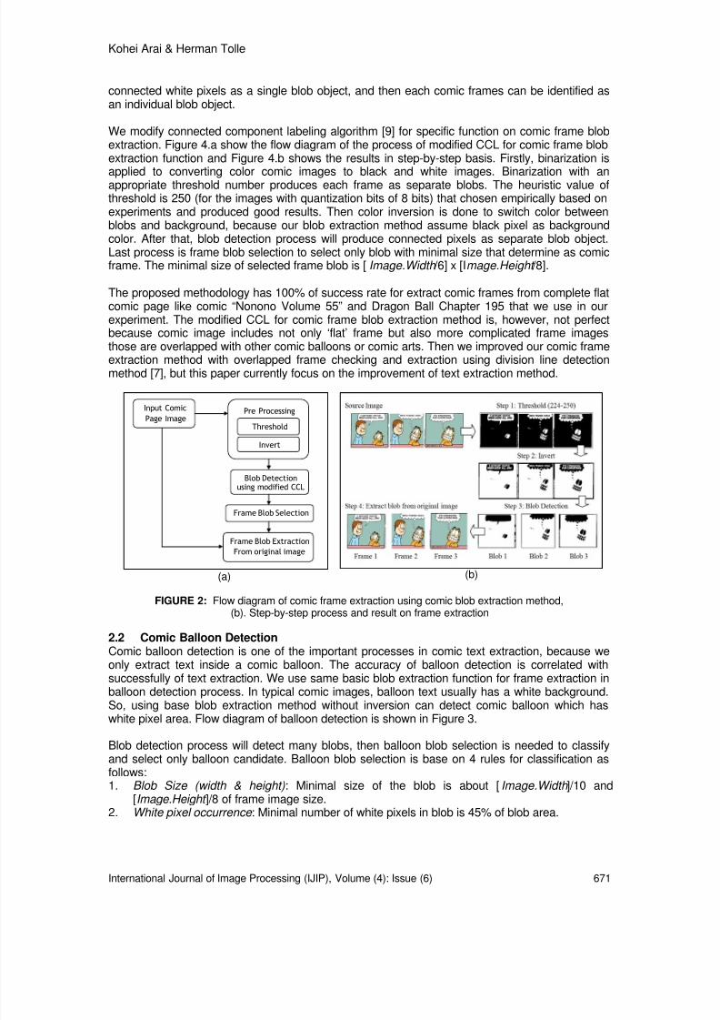
8/6/2019 International Journal of Image Processing (IJIP) Volume 4 Issue 6
http://slidepdf.com/reader/full/international-journal-of-image-processing-ijip-volume-4-issue-6 162/172
Kohei Arai & Herman Tolle
International Journal of Image Processing (IJIP), Volume (4): Issue (6) 671
connected white pixels as a single blob object, and then each comic frames can be identified asan individual blob object.
We modify connected component labeling algorithm [9] for specific function on comic frame blobextraction. Figure 4.a show the flow diagram of the process of modified CCL for comic frame blobextraction function and Figure 4.b shows the results in step-by-step basis. Firstly, binarization isapplied to converting color comic images to black and white images. Binarization with anappropriate threshold number produces each frame as separate blobs. The heuristic value ofthreshold is 250 (for the images with quantization bits of 8 bits) that chosen empirically based onexperiments and produced good results. Then color inversion is done to switch color betweenblobs and background, because our blob extraction method assume black pixel as backgroundcolor. After that, blob detection process will produce connected pixels as separate blob object.Last process is frame blob selection to select only blob with minimal size that determine as comicframe. The minimal size of selected frame blob is [ Image.Width /6] x [I mage.Height /8].
The proposed methodology has 100% of success rate for extract comic frames from complete flatcomic page like comic “Nonono Volume 55” and Dragon Ball Chapter 195 that we use in ourexperiment. The modified CCL for comic frame blob extraction method is, however, not perfectbecause comic image includes not only ‘flat’ frame but also more complicated frame imagesthose are overlapped with other comic balloons or comic arts. Then we improved our comic frameextraction method with overlapped frame checking and extraction using division line detectionmethod [7], but this paper currently focus on the improvement of text extraction method.
Pre ProcessingInput ComicPage Image
Threshold
Invert
Blob Detectionusing modified CCL
Frame Blob ExtractionFrom original image
Frame Blob Selection
(a) (b)
FIGURE 2: Flow diagram of comic frame extraction using comic blob extraction method,(b). Step-by-step process and result on frame extraction
2.2 Comic Balloon DetectionComic balloon detection is one of the important processes in comic text extraction, because weonly extract text inside a comic balloon. The accuracy of balloon detection is correlated withsuccessfully of text extraction. We use same basic blob extraction function for frame extraction inballoon detection process. In typical comic images, balloon text usually has a white background.So, using base blob extraction method without inversion can detect comic balloon which haswhite pixel area. Flow diagram of balloon detection is shown in Figure 3.
Blob detection process will detect many blobs, then balloon blob selection is needed to classifyand select only balloon candidate. Balloon blob selection is base on 4 rules for classification asfollows:1. Blob Size (width & height) : Minimal size of the blob is about [ Image.Width ]/10 and
[Image.Height ]/8 of frame image size.2. White pixel occurrence : Minimal number of white pixels in blob is 45% of blob area.

8/6/2019 International Journal of Image Processing (IJIP) Volume 4 Issue 6
http://slidepdf.com/reader/full/international-journal-of-image-processing-ijip-volume-4-issue-6 163/172
Kohei Arai & Herman Tolle
International Journal of Image Processing (IJIP), Volume (4): Issue (6) 672
3. Straight Line : At least two straight vertical white lines with 70% long of blob height size isdetected. One line in the half left and one in the half right.
4. Width to Length Ratio : Blob width size is less than 1.5 of blob height size.
Pre ProcessingInput ComicFrame i
Threshold
Morphology Filter
Blob Extraction
Ballon Blob Extraction
Feature Extraction
Balloon Blob Selection& Classification
(a)
Input Comic Frame After pre-processing
Blob Extraction & Selection
Balloon Detected Non Balloon Detected
(b)
FIGURE 3: Flow diagram of comic balloon detection using comic blob extraction method,(b). Step-by-step process and result on comic balloon detection
3. BLOB EXTRACTION BASED METHODOLOGY FOR TEXT EXTRACTIONThe objective of text extraction method is to extract Japanese text from comic balloon as singleblob object for same vertical sentence or word. This vertical direction word will useful forcharacter recognizing using optical character recognition (OCR) method which is out of this scopeat this time. The proposed methodology is blob extraction based or region based method, andoperates on digital comic image which has frame extraction and balloon detection processedpreviously. The text extraction method comprises of 5 phases; pre processing with binarizationand morphology filter, blob extraction, blob feature extraction, text blob selection andclassification, and the last process is text blob extraction. The block schematic of the textextraction methodology is given in Figure 4. The detailed description of each phase is presentedin the following subsections.
Pre ProcessingInput ComicBalloon
Threshold
Morphology Filter
Blob Extraction
Text Blob Extraction
Feature Extraction
Text Blob Selection &Classification

8/6/2019 International Journal of Image Processing (IJIP) Volume 4 Issue 6
http://slidepdf.com/reader/full/international-journal-of-image-processing-ijip-volume-4-issue-6 164/172
Kohei Arai & Herman Tolle
International Journal of Image Processing (IJIP), Volume (4): Issue (6) 673
FIGURE 4: Text Extraction Algorithm
3.1 Pre-ProcessingBefore extracted text blob from comic balloon, pre-processing filtering has to be done for preset
image into binary color. First, adaptive threshold method is applied to comic page image.Threshold value T is obtained from average pixel value of comic image µ . We set threshold valueis 30% above from the average empirically.
∑−
=
=
1
0
1N
i
i I N
µ
30.0 / µ =T
(1)
(2)
Then we implement a morphology filter in pre-processing to merge neighboring character blobimage as a single blob. In pre-processing, erosion filter and opening filter is applied with top andbottom side priority more than left and right side because Japanese character reading order inManga is from top to bottom. The block diagram and results sample of pre processing is given inFigure 4.
3.2 Blob ExtractionAfter pre-processing, we detect all connected pixels as a separate blob object. Blob extraction isdone using same blob extraction method with 2 previous processes to extract text blobscandidate from a comic balloon. This process produces text blobs and also non text blobs. Toclassify a blob as a text blob or non text blob, we extract some features from text blob candidatefor classification. In text blob extraction using blob extraction function, we select only blob withminimal size that selected as candidate of text blob. The minimal size of the text candidate blobwidth is [ Image.Width ]/20 and the text blob height is [ Image.Height ]/40. Parameter of [Image] corresponds to balloon blob image size as the input of process.
3.3 Text Blob Feature Extraction and ClassificationText blob classification is needed to classify text blob from extracted blobs into vertical (column)text region. Classification is based on the features of blob size and blob position. Classification
process classify text blob with the same column into same cluster as a representative ofJapanese classic sentence or word in column. To classify and combine text blob in verticaldirection, we extract some features from detected text blob. Features to extract are average text blob width and text blob x center point (TB.XCenter ). Average text blob width is needed todetermine distance between two columns of vertical text. Average text blob width is chosen fromaverage width of three blobs in the mean of blob after sorting all blob based on blob’s size. Text blob x center point is described in Equation 3. Text blob size of each blob is actual parameter ofblob object which is containing top and left position parameter, and width and height parameter.
TB[i].XCenter = TB[i].Left + (TB[i].Width / 2) (3)
Where;TB[i] corresponds to i th blob of detected text blob.TB[i].Left corresponds to left point position parameter of detected text blob TB[i].Width corresponds to width parameter of detected text blob
For selecting and classifying text blob into vertical text region, we use 2 rules for classification asfollows:1. Blob position is not related with balloon blob border. Assuming minimal distance is d min .2. Classify blob with same vertical center point in same cluster. Assuming difference distance
between centers is BD min .If (TB[i].XCenter +- BD min ) ∈ Column[j] Then TB[i] member of Column[j]

8/6/2019 International Journal of Image Processing (IJIP) Volume 4 Issue 6
http://slidepdf.com/reader/full/international-journal-of-image-processing-ijip-volume-4-issue-6 165/172
Kohei Arai & Herman Tolle
International Journal of Image Processing (IJIP), Volume (4): Issue (6) 674
Minimal distance from border d min is approximately 5% pixels from balloon edge and minimaldistance BD min is approximately less than half of average text blob width.
3.4 Text Blob ExtractionLast step on text extraction method is text blob extraction from original balloon image based ontext blob cluster from previous process. In classification process, each blob in same cluster is
combining as a new blob as representative of text in vertical. Then using the position of newblobs, text candidate is extracted from original balloon text image from input process. Figure 5show step by step process and results of manga text extraction algorithm. The final result is set oftext blob that represent Japanese sentence from comic text balloon in vertical direction. Thoseimage blobs than store in database or directly proceed to OCR application for text recognition.
1 2 3 4 5
a b c d eFIGURE 5: Sample of Text Extraction Process
(a) Original balloon text image; (b) Threshold; (c) Morphology-Erosion filter;(d) Morphology-Opening filter; (e) Extracted blob from original image
4. EXPERIMENTSThe proposed methodology for extracted Japanese character from digital comic image has beenevaluated using various comic image pages. We implement the proposed method usingMicrosoft.Net environment with C# as native language and AForge image processing frameworkon desktop computer with Pentium Dual Core processor and 1 mega byte of RAM. Experiment isconducting through 15 comic pages to evaluate the success rate (accuracy) of text extraction.Common comic image size that we use in our experiment is 800x1200 pixels. The results of theexperiment then reported and compared with other methods.
4.1 Experimental ResultsPerformance evaluation of proposed methods on frame extraction, balloon detection and textextraction is evaluated for 15 comic pages from Dragon Ball Chapter 195 Japanese version. Thiscomic contains 15 pages with 60 frames, 70 comic balloons and 160 columns of Japanesesentences. Experimental result of balloon detection and text extraction method has shown inTable 1. The results were classified into 3 groups such as “ correctly extraction ” (T ), “missed detection ” (M ) and “ false detection ” (F ). In the case of frame extraction, the term correctly extraction means the number of true detection of frames; missed detection means that there areframe that not detected by system; and the terms false detection means that some non framesare detected as frame. We also use the same interpretation on T , M and F for balloon detectionand text extraction process. In Table 1, there are 2 methods, base method and modified method.
Base method is our method which is explained in previous chapter, while modified method isbase method with modification. Detail of modified method explained in Discussion on next subchapter. From the experimental results, 100% of success rate of frame extraction method, 100%of success rate of comic balloon detection method and 93.75% of success rate of manga textextraction methods is achieved.
Table 1. Comic Balloon and Text Extraction experimental results
Comic Content Total T M F %Frame Extraction 60 60 0 0 100

8/6/2019 International Journal of Image Processing (IJIP) Volume 4 Issue 6
http://slidepdf.com/reader/full/international-journal-of-image-processing-ijip-volume-4-issue-6 166/172
Kohei Arai & Herman Tolle
International Journal of Image Processing (IJIP), Volume (4): Issue (6) 675
Balloon Detection based method 70 70 0 53 100Balloon Detection with modification 70 70 0 7 100Text Extraction 160 150 10 6 93.75
Time consuming in processing is main issue in real time online application. We evaluateprocessing time of our method in offline simulation for each process on comic text extractionwithout text recognition process. The result of processing time evaluation is shown in Table 2,with comparison with other method. Processing time experimental results shows that ourproposed method is faster that other method. Comparing with conventional method, processingtime of our method is about 90% faster than conventional method. Online situation need moreprocessing time consuming rather than offline situation because of another processing within thesystems, but still acceptable as online application.
Table 2. Processing time experimental results and comparison
Comic PageProcessing Time (minutes)
ConventionalMethod Our Method
15 comic page offlinewith 70 balloon Approx. > 30 2.5
4.2 DiscussionAlthough our base method for balloon detection and text extraction has performed good resultson correctly extraction , it still has a lot of false detection. In balloon detection method, there are alot of non balloon detected as balloon candidates. It causes by the form of comic image that lookslike balloon and pass our selection criteria. To reducing false detection, we make a simplemodification for balloon detection criteria by adding one process. The new process is performingtext detection on balloon candidate. If a candidate of text detected inside a balloon candidate,then classify it as a new balloon candidate. If there is no text blob candidate detected inside aballoon, then classify it as a non balloon. Implementing of this modified method, reduce about90% of false detection. Figure 6 shows the sample of false detection of balloon candidate, whicheliminated on text detection. Actually, the occurrence of false detection in text extraction processis not a serious problem because in the next process while we implement OCR for extract textfrom text blob image, the false detected of balloon or text produces nothing after OCR
processing. In the other hand, the accuracy of text extraction method is 93.75% while 6.25% oftexts are not detected or system fail to detect and extract. Most of the failure on text extraction iscause by non standard of position of the character within a balloon as shown in Figure 6.b.System also fail to extract 2 or more text column that close to another.
Implementation of our method is possible in offline or online real time basis because the simplicityof the program code and fast processing time. By using our method, vertical Japanese sentencein a comic balloon is easy to extract then recognized for language translation. We can create amobile application for reading comic with language translation process by implementing of ourmethod combine with OCR feature and Google Language Translation tool using mobileprogramming framework like Android or another framework.
(a) (b)FIGURE 6: (a) Sample of non balloon detected as a balloon candidate (false detection);
(b) sample of miss detection text

8/6/2019 International Journal of Image Processing (IJIP) Volume 4 Issue 6
http://slidepdf.com/reader/full/international-journal-of-image-processing-ijip-volume-4-issue-6 167/172
Kohei Arai & Herman Tolle
International Journal of Image Processing (IJIP), Volume (4): Issue (6) 676
5. CONCLUSION & FUTURE WORKWe implemented a system for automatically extract Japanese character from digital manga comicimage. Our proposed method can automatically detect comic frame and detect all balloon within acomic frame. After all balloon detected, then system will extract Japanese character text inside aballoon as comic dialog in Japanese language for further purpose especially for languagetranslation. The proposed method on Japanese character text extraction is possible to implement
in offline or online real time basis so it is possible to become an online application for languagetranslation. From the experimental results, our comic frame extraction method has 100%accuracy for flat comic, balloon detection method achieves 100% accuracy and text extractionmethod achieves 93.75% accuracy.
Combining the proposed method with our e-comic content adaptation system, will create a robustsystem for automatically convert digital comic image from comic web portal into mobile contentwith language translation features. We will improve this current method with implementingcharacter recognition function in the systems. Also for further work, we will implement anapplication for automatically convert Japanese comic into international comic for enjoy readingcomic anywhere anytime using mobile phones.
6. REFERENCES1. L. Fletcher and R. Kasturi, A robust algorithm for text string separation from mixedtext/graphics images. IEEE Trans. Pattern Anal. Mach. Intell. 10 (1988), pp. 910–918
2. A.K. Jain and B. Yu, Automatic text location in images and video frames. PatternRecognition 31 12 (1998), pp. 2055–2076
3. O. Iwaki, K. Kubota and H. Arakawa, A character/graphic segmentation method usingneighborhood line density. IEICE Trans. Inform. Process. J68 4 (1985), pp. 821–828.
4. L.A. Fletcher and R. Kasturi, A robust algorithm for text string separation from mixedtext/graphics images. IEEE Trans. Pattern Analysis Mach. Intell. 10 6 (1988), pp. 910–918
5. Eunjung Han, et.al. “Automatic Mobile Content Conversion Using Semantic Image Analysis”,Human-Computer Interaction HCI Intelligent Multimodal Interaction Environments, LNCS4552, Springer, Berlin, 2007
6. Yamada, M., Budiarto, R. and Endoo, M., “Comic image decomposition for Reading comicson cellular phones”. IEICE transaction on information and systems, E-87-D (6):1370-1376,June 2004.
7. Kohei Arai, Tolle Herman, "Method for Automatic E-Comic Scene Frame Extraction forReading Comic on Mobile Devices," itng, pp.370-375, 2010 Seventh International Conferenceon Information Technology, 2010
8. Kohei, A., Tolle, H., “Automatic E-Comic Content Adaptation”, International Journal ofUbiquitous Computing IJUC Volume (1): Issue (1), May 2010.
9. F. Chang, C-J. Chen and C-J. Lu. “A Linear-Time Component-Labeling Algorithm UsingContour Tracing Technique”, Computer Vision and Image Understanding, 93(2):pp. 206-220,2004.
10. R. Gonzalez and R. Woods. “Digital Image Processing”, Addison-Wesley Chap.2., PublishingCompany (1992)

8/6/2019 International Journal of Image Processing (IJIP) Volume 4 Issue 6
http://slidepdf.com/reader/full/international-journal-of-image-processing-ijip-volume-4-issue-6 168/172
CALL FOR PAPERS
Journal : International Journal of Image Processing (IJIP)Volume : 5 Issue : 1ISSN :1985-2304URL : http://www.cscjournals.org/csc/description.php?JCode=IJIP
About IJIPThe International Journal of Image Processing (IJIP) aims to be an effectiveforum for interchange of high quality theoretical and applied research in theImage Processing domain from basic research to application development. Itemphasizes on efficient and effective image technologies, and provides acentral forum for a deeper understanding in the discipline by encouraging thequantitative comparison and performance evaluation of the emergingcomponents of image processing.
We welcome scientists, researchers, engineers and vendors from differentdisciplines to exchange ideas, identify problems, investigate relevant issues,share common interests, explore new approaches, and initiate possiblecollaborative research and system development.
To build its International reputation, we are disseminating the publicationinformation through Google Books, Google Scholar, Directory of Open AccessJournals (DOAJ), Open J Gate, ScientificCommons, Docstoc and many more.Our International Editors are working on establishing ISI listing and a goodimpact factor for IJIP.
IJIP List of Topics
The realm of International Journal of Image Processing (IJIP) extends, butnot limited, to the following:
• Architecture of imaging and visionsystems
• Autonomous vehicles
• Character and handwritten textrecognition
• Chemical and spectralsensitization
• Chemistry of photosensitive materials • Coating technologies• Coding and transmission • Cognitive aspects of image
understanding• Color imaging • Communication of visual data• Data fusion from multiple sensor inputs • Display and printing• Document image understanding • Generation and display• Holography • Image analysis and
interpretation• Image capturing, databases • Image generation, manipulation,
permanence• Image processing applications • Image processing: coding

8/6/2019 International Journal of Image Processing (IJIP) Volume 4 Issue 6
http://slidepdf.com/reader/full/international-journal-of-image-processing-ijip-volume-4-issue-6 169/172
analysis and recognition• Image representation, sensing • Imaging systems and image
scanning• Implementation and architectures • Latent image• Materials for electro-photography • Network architecture for real-
time video transport• New visual services over ATM/packet
network• Non-impact printing
technologies• Object modeling and knowledge
acquisition• Photoconductors
• Photographic emulsions • Photopolymers• Prepress and printing technologies • Protocols for packet video• Remote image sensing • Retrieval and multimedia• Storage and transmission • Video coding algorithms and
technologies for ATM/p
IMPORTANT DATES
Volume: 5Issue: 1Paper Submission: January 31, 2011Author Notification: March 01, 2011Issue Publication: March /April 2011

8/6/2019 International Journal of Image Processing (IJIP) Volume 4 Issue 6
http://slidepdf.com/reader/full/international-journal-of-image-processing-ijip-volume-4-issue-6 170/172
CALL FOR EDITORS/REVIEWERS
CSC Journals is in process of appointing Editorial Board Members for International Journal of Image Processing (IJIP) . CSC Journalswould like to invite interested candidates to join IJIP network of professionals/researchers for the positions of Editor-in-Chief, AssociateEditor-in-Chief, Editorial Board Members and Reviewers.
The invitation encourages interested professionals to contribute intoCSC research network by joining as a part of editorial board membersand reviewers for scientific peer-reviewed journals. All journals use anonline, electronic submission process. The Editor is responsible for thetimely and substantive output of the journal, including the solicitationof manuscripts, supervision of the peer review process and the finalselection of articles for publication. Responsibilities also includeimplementing the journal’s editorial policies, maintaining highprofessional standards for published content, ensuring the integrity of the journal, guiding manuscripts through the review process,overseeing revisions, and planning special issues along with theeditorial team.
A complete list of journals can be found athttp://www.cscjournals.org/csc/byjournal.php. Interested candidatesmay apply for the following positions throughhttp://www.cscjournals.org/csc/login.php.
Please remember that it is through the effort of volunteers such asyourself that CSC Journals continues to grow and flourish. Your help
with reviewing the issues written by prospective authors would be very much appreciated.
Feel free to contact us at [email protected] if you have anyqueries.

8/6/2019 International Journal of Image Processing (IJIP) Volume 4 Issue 6
http://slidepdf.com/reader/full/international-journal-of-image-processing-ijip-volume-4-issue-6 171/172
Contact Information
Computer Science Journals Sdn BhDM-3-19, Plaza Damas Sri Hartamas
50480, Kuala Lumpur MALAYSIAPhone: +603 6207 1607
+603 2782 6991Fax: +603 6207 1697
BRANCH OFFICE 1Suite 5.04 Level 5, 365 Little Collins Street,MELBOURNE 3000, Victoria, AUSTRALIA
Fax: +613 8677 1132
BRANCH OFFICE 2Office no. 8, Saad Arcad, DHA Main BulevardLahore, PAKISTAN
EMAIL SUPPORTHead CSC Press: [email protected] Press: [email protected]: [email protected]

8/6/2019 International Journal of Image Processing (IJIP) Volume 4 Issue 6
http://slidepdf.com/reader/full/international-journal-of-image-processing-ijip-volume-4-issue-6 172/172