International Journal of Engineering Science 47 (2009) 141–152

Contents lists available at ScienceDirect

International Journal of Engineering Science

journal homepage: www.elsevier .com/locate / i jengsci

Annular axisymmetric stagnation flow on a moving cylinder

Liu Hong a, C.Y. Wang b,*

a Zhou Pei-Yuan Center for Applied Mathematics, Tsinghua University, Beijing, Chinab Departments of Mathematics and Mechanical Engineering, Michigan State University, Abbott Road, East Lansing, MI 48824, USA

a r t i c l e i n f o a b s t r a c t

Article history:Received 23 January 2008Received in revised form 11 August 2008Accepted 13 August 2008Available online 25 September 2008

Communicated by K.R. Rajagopal

Keywords:Stagnation flowCylinderSimilarity

0020-7225/$ - see front matter � 2008 Elsevier Ltddoi:10.1016/j.ijengsci.2008.08.002

* Corresponding author.E-mail address: cywang@mth.msu.edu (C.Y. Wan

Fluid is injected from a fixed outer cylindrical casing onto an inner moving cylindrical rod.Using similarity transform, the Navier–Stokes equations reduce to a set of nonlinear ordin-ary differential equations, which are integrated numerically. Asymptotic solutions for largeand small cross-flow Reynolds numbers and small gap widths are also found. Drag, torqueand heat transfer on the moving rod are determined. The problem is particularly importantin pressure-lubricated bearings.

� 2008 Elsevier Ltd. All rights reserved.

1. Introduction

Similarity solutions of the Navier–Stokes equations are rare [1]. The basic similarity solution describing two-dimensionalstagnation flow towards a plate was introduced by Hiemenz [2]. The similarity solution for the axisymmetric stagnation flowon a circular cylinder was found by Wang [3]. Gorla [4] extended the solution to include axial translation of the cylinderwhile Cunning et al. [5] studied the axial rotation and transpiration on the cylinder. The previous literature considered astagnation flow originated from infinity. In the present paper, the stagnation flow in the annular region between two cylin-ders is studied. Fluid is injected inward radially from a fixed outer cylinder towards an axially translating and rotating innercylinder. Such finite geometry is more realistic for the convective cooling of a moving rod [6]. The problem also models exter-nally pressure-lubricated journal bearings which are quite attractive for high speed and miniature rotating systems [7–11].The aim of the present paper is to find a similarity stagnation flow for the annular region.

2. Formulation

Fig. 1 shows a vertical inner cylinder (shaft) of radius R rotating with angular velocity X and moving with velocity W inthe axial z-direction. The inner cylinder is enclosed by an outer cylinder (bushing) of radius bR. Fluid is injected radially withvelocity U from the outer cylinder towards the inner cylinder. Assuming end effects can be ignored (long cylinders), the flowis axisymmetric about the z-axis.

The constant property continuity equation and the constant property Navier–Stokes equations in axisymmetric cylindri-cal coordinates are:

. All rights reserved.

g).

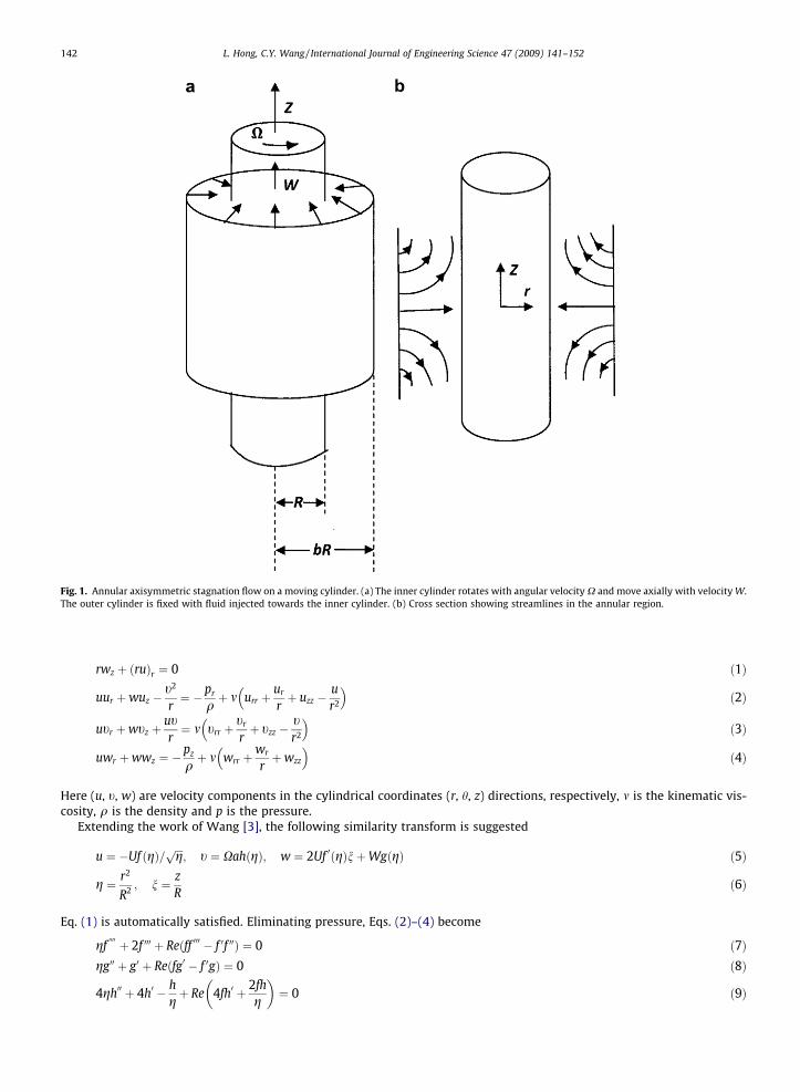
Fig. 1. Annular axisymmetric stagnation flow on a moving cylinder. (a) The inner cylinder rotates with angular velocity X and move axially with velocity W.The outer cylinder is fixed with fluid injected towards the inner cylinder. (b) Cross section showing streamlines in the annular region.

142 L. Hong, C.Y. Wang / International Journal of Engineering Science 47 (2009) 141–152

rwz þ ðruÞr ¼ 0 ð1Þ

uur þwuz �t2

r¼ �pr

qþ m urr þ

ur

rþ uzz �

ur2

� �ð2Þ

utr þwtz þutr¼ m trr þ

tr

rþ tzz �

tr2

� �ð3Þ

uwr þwwz ¼ �pz

qþ m wrr þ

wr

rþwzz

� �ð4Þ

Here (u, t, w) are velocity components in the cylindrical coordinates (r, h, z) directions, respectively, m is the kinematic vis-cosity, q is the density and p is the pressure.

Extending the work of Wang [3], the following similarity transform is suggested

u ¼ �Uf ðgÞ= ffiffiffigp

; t ¼ XahðgÞ; w ¼ 2Uf 0ðgÞnþWgðgÞ ð5Þ

g ¼ r2

R2 ; n ¼ zR

ð6Þ

Eq. (1) is automatically satisfied. Eliminating pressure, Eqs. (2)–(4) become

gf0000 þ 2f 000 þ Reðff 000 � f 0f 00Þ ¼ 0 ð7Þ

gg00 þ g0 þ Reðfg0 � f 0gÞ ¼ 0 ð8Þ

4gh00 þ 4h0 � hgþ Re 4fh0 þ 2fh

g

� �¼ 0 ð9Þ

L. Hong, C.Y. Wang / International Journal of Engineering Science 47 (2009) 141–152 143

Here Re = Ua/2m is the cross-flow Reynolds number. The pressure can be recovered by

p ¼ ps � qU2f 2

2gþ U2f 0

Re�X2R2

2

Z g

1

h2ðsÞs

dsþ 2C0U2n2

" #ð10Þ

where ps is the stagnation pressure, and C0 = f000(1) + f00(1). The boundary conditions are no slip on the inner cylinder

f ð1Þ ¼ 0; f 0ð1Þ ¼ 0 ð11Þgð1Þ ¼ 1; hð1Þ ¼ 1 ð12Þ

and uniform injection on the outer cylinder

f ðbÞ ¼ffiffiffibp

; f 0ðbÞ ¼ 0 ð13ÞgðbÞ ¼ 0; hðbÞ ¼ 0 ð14Þ

Although Eqs. (7), (11) and (13) are decoupled from the other equations, the system is still formidable. In what follows weshall develop some approximate solutions before integrating the similarity equations Eqs. (7)–(9) and (11)–(14) numerically.

3. Asymptotic solution for small Reynolds numbers

This is the case when the injection velocity is small, or the diameter of the inner cylinder is small, or the viscosity is large.We expand in terms of Reynolds number Re� 1.

f ¼ f0 þ Ref1 þ � � � ð15Þg ¼ g0 þ Reg1 þ � � � ; h ¼ h0 þ Reh1 þ � � � ð16Þ

Eqs. (7)–(9) lead to the zeroth order equations

gf0000

0 þ 2f 0000 ¼ 0 ð17Þgg000 þ g00 ¼ 0 ð18Þ

4gh000 þ 4h00 �h0

g¼ 0 ð19Þ

with the boundary conditions

f0ð1Þ ¼ f 00ð1Þ ¼ f 00ðbÞ ¼ 0; f 0ðbÞ ¼ffiffiffibp

ð20Þg0ð1Þ ¼ 1; g0ðbÞ ¼ 0 ð21Þh0ð1Þ ¼ 1; h0ðbÞ ¼ 0 ð22Þ

The solutions are

f0 ¼ffiffiffibp½�2ðb� 1Þg ln gþ ln b � g2 þ 2ðb� 1� ln bÞg� ð2b� 2� ln bÞ�

ðb� 1Þ½2ðb� 1Þ � ðbþ 1Þ ln b� ð23Þ

g0 ¼ �ln gln bþ 1 ð24Þ

h0 ¼g� b

ð1� bÞ ffiffiffigp ð25Þ

The first order equations are

gf0000

1 þ 2f 0001 ¼ f 00f 000 � f0f 0000 ð26Þgg001 þ g01 ¼ f 00g0 � f0g00 ð27Þ

4gh001 þ 4h01 �h1

g¼ �4f 0h00 �

2f 0h0

gð28Þ

with zero boundary conditions. The solutions are complicated but straight forward, and will not be presented here (seeAppendix). However, they are used in the comparison with the exact numerical solution in a later section. Fig. 2 shows sometypical profiles of the first order functions. The Appendix gives the analytic forms obtained by a computer with symboliccapability.

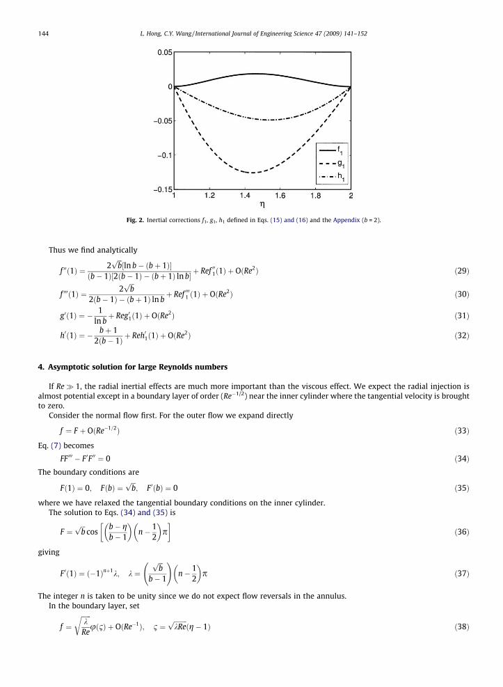
Fig. 2. Inertial corrections f1, g1, h1 defined in Eqs. (15) and (16) and the Appendix (b = 2).

144 L. Hong, C.Y. Wang / International Journal of Engineering Science 47 (2009) 141–152

Thus we find analytically

f 00ð1Þ ¼ 2ffiffiffibp½ln b� ðbþ 1Þ�

ðb� 1Þ½2ðb� 1Þ � ðbþ 1Þ ln b� þ Ref 001ð1Þ þ OðRe2Þ ð29Þ

f 000ð1Þ ¼ 2ffiffiffibp

2ðb� 1Þ � ðbþ 1Þ ln bþ Ref 0001 ð1Þ þ OðRe2Þ ð30Þ

g0ð1Þ ¼ � 1ln bþ Reg01ð1Þ þ OðRe2Þ ð31Þ

h0ð1Þ ¼ � bþ 12ðb� 1Þ þ Reh01ð1Þ þ OðRe2Þ ð32Þ

4. Asymptotic solution for large Reynolds numbers

If Re� 1, the radial inertial effects are much more important than the viscous effect. We expect the radial injection isalmost potential except in a boundary layer of order (Re�1/2) near the inner cylinder where the tangential velocity is broughtto zero.

Consider the normal flow first. For the outer flow we expand directly

f ¼ F þ OðRe�1=2Þ ð33Þ

Eq. (7) becomes

FF 000 � F 0F 00 ¼ 0 ð34Þ

The boundary conditions are

Fð1Þ ¼ 0; FðbÞ ¼ffiffiffibp

; F 0ðbÞ ¼ 0 ð35Þ

where we have relaxed the tangential boundary conditions on the inner cylinder.The solution to Eqs. (34) and (35) is

F ¼ffiffiffibp

cosb� gb� 1

� �n� 1

2

� �p

� �ð36Þ

giving

F 0ð1Þ ¼ ð�1Þnþ1k; k ¼ffiffiffibp

b� 1

!n� 1

2

� �p ð37Þ

The integer n is taken to be unity since we do not expect flow reversals in the annulus.In the boundary layer, set

f ¼ffiffiffiffiffiffik

Re

ruð1Þ þ OðRe�1Þ; 1 ¼

ffiffiffiffiffiffiffiffikRep

ðg� 1Þ ð38Þ

L. Hong, C.Y. Wang / International Journal of Engineering Science 47 (2009) 141–152 145

Then Eqs. (7), (11) and (13) yield the Hiemenz boundary layer equation

Fig. 3.

u000 þuu00 �u02 þ 1 ¼ 0 ð39Þuð0Þ ¼ u0ð0Þ ¼ 0; u0ð1Þ ¼ 1 ð40Þ

The solution to Eqs. (39) and (40) is well known (e.g. [12]). We find

u00ð0Þ ¼ 1:232588; uð1Þ � 1� 0:6479 ð41Þ

A uniformly valid solution is then constructed

f ¼ffiffiffibp

cosb� gb� 1

� �p2

� �þ

ffiffiffiffiffiffik

Re

r½uð1Þ � 1� þ � � � ð42Þ

From which we find the boundary derivatives

f 00ð1Þ ¼ kffiffiffiffiffiffiffiffikRep

u00ð0Þ ¼ 1:232588kffiffiffiffiffiffiffiffikRep

ð43Þ

f 000ð1Þ ¼ �k2Re� k3

bþ � � � ð44Þ

Similarly, let

g ¼ Gþ OðRe�1=2Þ; h ¼ H þ OðRe�1=2Þ ð45Þ

The outer flow yields

G ¼ 0; H ¼ 0 ð46Þ

In the boundary layer, let

g ¼ wð1Þ; h ¼ hð1Þ ð47Þ

And from Eqs. (8) and (9) we obtain the boundary layer equations

w00 þuw0 �u0w ¼ 0 ð48Þh00 þuh0 ¼ 0 ð49Þ

The boundary conditions are

wð0Þ ¼ 1; wð1Þ ¼ 0 ð50Þhð0Þ ¼ 1; hð1Þ ¼ 0 ð51Þ

Since the function for u is known, Eqs. (48)–(51) are integrated numerically, resulting in universal (no parameter depen-dence) solutions for w and h. We find w0(0) = �0.81130 and h0(0) = �0.57045. Thus the analytic boundary derivatives are

g0ð1Þ ¼ �0:81130ffiffiffiffiffiffiffiffikRep

þ � � � ð52Þh0ð1Þ ¼ �0:57045

ffiffiffiffiffiffiffiffikRep

þ � � � ð53Þ

The universal curves of u, w, and h are shown in Fig. 3.

The universal curves of u, w, and h. u is the Hiemenz solution, w and h are functions due to the motion of the inner cylinder. See Eqs. (5) and (47).

146 L. Hong, C.Y. Wang / International Journal of Engineering Science 47 (2009) 141–152

5. Perturbation solution for small gap width

This case models bearings with fluid injection. When the annulus gap width is small, set e = b � 1� 1 and

g ¼ 1þ er; 0 6 r 6 1 ð54Þ

Expand

f ¼ U0ðrÞ þ eU1ðrÞ þ � � � ; g ¼ W0ðrÞ þ eW1ðrÞ þ � � � ; h ¼ K0ðrÞ þ eK1ðrÞ þ � � � ð55Þ

We assume the cross-flow Reynolds number is not too large. Eqs. (7)–(9) and (11)–(14) yield the zeroth order

U0000

0 ¼ 0; W000 ¼ 0; K000 ¼ 0 ð56Þ

with the boundary conditions

U0ð0Þ ¼ 1; U00ð0Þ ¼ 0; U0ð1Þ ¼ 1; U00ð1Þ ¼ 0 ð57ÞW0ð0Þ ¼ 1; W0ð1Þ ¼ 0; K0ð0Þ ¼ 1; K0ð1Þ ¼ 0 ð58Þ

The solutions are

U0 ¼ 3r2 � 2r3; W0 ¼ 1� r; K0 ¼ 1� r ð59Þ

The first order equations are

U0000

1 ¼ �2U0000 � ReðU0U0000 �U00U

000Þ ð60Þ

W001 ¼ �W00 � ReðU0W00 �U00W0Þ ð61Þ

K001 ¼ �K00 � ReU0K00 ð62Þ

With the boundary conditions

U1ð0Þ ¼ 0; U01ð0Þ ¼ 0; U1ð1Þ ¼ 1=2; U01ð1Þ ¼ 0 ð63ÞW1ð0Þ ¼ 0; W1ð1Þ ¼ 0; K1ð0Þ ¼ 0; K1ð1Þ ¼ 0 ð64Þ

The solutions are

U1 ¼52r2 � 3r3 þ r4 þ Re

835

r2 � 2770

r3 þ 310

r5 � 15r6 þ 2

35r7

� �ð65Þ

W1 ¼ �12rþ 1

2r2 þ Re � 9

20rþ r3 þ 3

10r5 � 3

4r4 þ 1

5r5

� �ð66Þ

K1 ¼ �12rþ 1

2r2 þ Re � 3

20rþ 1

4r4 � 1

10r5

� �ð67Þ

The approximate boundary derivatives are then

f 00ð1Þ ¼ 1e2 U000ð0Þ þ eU001ð0Þ þ � � �

¼ 1e2 6þ e 5þ 16

35Re

� �þ � � �

� �ð68Þ

f 000ð1Þ ¼ 1e3 U0000 ð0Þ þ eU0001 ð0Þ þ � � �

¼ 1e3 �12� e 18þ 81

35Re

� �þ � � �

� �ð69Þ

g0ð1Þ ¼ 1e

W000ð0Þ þ eW001ð0Þ þ � � �

¼ 1e�1� e

12þ 9

20Re

� �þ � � �

� �ð70Þ

h0ð1Þ ¼ 1e

K000ð0Þ þ eK001ð0Þ þ � � �

¼ 1e�1� e

12þ 3

20Re

� �þ � � �

� �ð71Þ

6. Numerical solution and comparison of results

The exact numerical integration of the similarity equations is described as follows. Given the cross-flow Reynolds numberRe and the gap width b � 1 > 0, together with a guessed boundary derivatives for f00(1) and f000(1), Eq. (7) is integrated as aninitial value problem by a standard Runge–Kutta algorithm. The boundary derivatives are guided by our analytic approxi-mate solutions. When g = b we check whether Eq. (13) is satisfied. Through two-dimensional shooting with Newton’s cor-rection, one can obtain the boundary derivatives fairly accurately. The relative error is kept under 10�6. Then using thesolution for f, we integrate either Eq. (8) or Eq. (9) for the functions g or h. The initial conditions are Eq. (12) with a guessedg0(1) or h0(1). The solution is found when Eq. (14) is satisfied. Some representative curves for the functions f, g, h are given inFigs. 4–6. Our numerical solution of the ordinary differential equations, similar to Hiemenz’s [2] work, constitutes an exactsimilarity solution of the Navier–Stokes equations.

Fig. 4. Similarity function f(g) under different Reynolds numbers, numerically integrated with b = 2.

Fig. 5. Similarity function g(g) under different Reynolds numbers, numerically integrated with b = 2.

Fig. 6. Similarity function h(g) under different Reynolds numbers, numerically integrated with b = 2.

L. Hong, C.Y. Wang / International Journal of Engineering Science 47 (2009) 141–152 147

Table 1The boundary derivatives f00(1), f000(1), g0(1), h0(1)

f00(1) b = 1.1 b = 2 b = 10

Re Numer Small Re Large Re Small gap Numer Small Re Large Re Small gap Numer Small Re Large Re Small gap

0.1 650.3526 650.352 650.457 11.0010 11.001 11.0457 0.667 0.6674 0.6341 654.7679 654.770 654.571 11.6772 11.684 11.4571 0.863 0.8938 0.68010 698.6176 698.951 695.714 17.5348 18.519 15.5714 1.867 1.598100 1082.300 1140.800 824.218 1107.100 44.4492 40.810 5.292 5.0541000 2819.700 2606.400 132.436 129.053 16.210 15.98210000 8447.300 8242.200 411.373 408.103 50.764 50.539

f000(1) b = 1.1 b = 2 b = 10

Re Numer Small Re Large Re Small gap Numer Small Re Large Re Small gap Numer Small Re Large Re Small gap

0.1 �13883 �13883 �13823 �36.1443 �36.143 �30.2314 �0.9172 �0.917 �0.2411 �14117 �14116 �14031 �41.0797 �41.000 �32.3143 �1.3924 �1.405 �0.26710 �16507 �16452 �16114 �93.5670 �89.565 �5.2400 �6.287100 �42933 �39806 �36943 �590.738 �575.21 �36.4750 �30.4781000 �305970 �273350 �275480 �245230 �5211.80 �5431.7 �4940.30 �322.795 �304.6310000 �2813200 �2718200 �50187.0 �49354.0 �3102.90 �3046.2

g0(1) b = 1.1 b = 2 b = 10

Re Numer Small Re Large Re Small gap Numer Small Re Large Re Small gap Numer Small Re Large Re Small gap

0.1 �10.5382 �10.538 �10.545 �1.4963 �1.496 �1.545 �0.5080 �0.514 �0.6561 �10.9489 �10.948 �10.950 �1.9309 �1.984 �1.950 �0.9040 �1.234 �1.06110 �14.6586 �14.658 �15.000 �4.3856 �3.823 �6.000 �2.2168 �1.906100 �35.7103 �35.710 �32.929 �12.6450 �12.092 �6.3381 �6.0271000 �106.9611 �106.961 �104.133 �38.7853 �38.238 �19.3699 �19.05910000 �332.1775 �329.299 �121.452 �120.920 �60.5821 �60.272

h0(1) b = 1.1 b = 2 b = 10

Re Numer Small Re Large Re Small gap Numer Small Re Large Re Small gap Numer Small Re Large Re Small gap

0.1 �10.5151 �10.515 �10.515 �1.5151 �1.515 �1.515 �0.6235 �0.623 �0.6261 �10.6511 �10.650 �10.650 �1.6554 �1.650 �1.650 �0.7570 �0.731 �0.76110 �12.0407 �12.007 �12.000 �3.0517 �3.007 �2.7056 �3.000 �1.5941 �1.809 �1.348100 �24.8226 �25.570 �23.300 �25.500 �8.8636 �8.5559 �4.4487 �4.2641000 �75.1076 �73.681 �27.2421 �27.0562 �13.5959 �13.48610000 �233.5209 �231.540 �85.3916 �85.0227 �42.5694 �42.379

Values from exact numerical integration are compared with those from small Reynolds number approximation, large Reynolds number approximation andsmall gap approximation.

148 L. Hong, C.Y. Wang / International Journal of Engineering Science 47 (2009) 141–152

Table 1 shows a comparison of the exact numerical initial values thus obtained and the initial values using our analyticapproximate values. We see that the small Reynolds number approximation, Eqs. (29)–(32) is satisfactory for Re < 1, and therange may be extended to larger Re in certain cases. The large Reynolds number approximation, Eqs. (43), (44), (52) and (53)are good mostly for Re P 1000. On the other hand, the small gap width approximation, Eqs. (68)–(71) compares well if b < 2and moderate Reynolds numbers (we assumed Re = O(1) in the expansions).

From Eq. (1) a stream function v can be defined

u ¼ �1r

ovoz; w ¼ 1

rovor

ð72Þ

Using Eq. (5) we find

vR2U=2

¼ 2f ðgÞnþ aZ g

1gðgÞdg ð73Þ

Here a = W/U is the ratio of axial velocity to injection velocity. Figs. 7 and 8 show some representative streamlines. It is seenthat any axial motion of the cylinder skews the streamline pattern.

The longitudinal shear stress on the inner cylinder sl is given as

sl

2lU=R¼ 2f 00ð1Þnþ ag0ð1Þ ð74Þ

where l = qm is the dynamic viscosity of the fluid. The azimuthal shear stress sa is found to be

sa

lX¼ 2h0ð1Þ � 1 ð75Þ

Fig. 7. The normalized stream function vR2 U=2

with b = 2, Re = 1,a = 0. Fluid is injected from the outer cylinder at g = 2 towards the inner cylinder at g = 1. Thedashed line stands for the stagnation streamline.

Fig. 8. The normalized stream function vR2 U=2

with b = 2, Re = 1, a = 3.

L. Hong, C.Y. Wang / International Journal of Engineering Science 47 (2009) 141–152 149

Let D be the longitudinal drag and L be the length of the annulus. Integrating Eq. (74) over the inner surface gives

DpLlW

¼ 4g0ð1Þ ð76Þ

Let M be the moment or toque experienced by the rotation. Then

M

pLR2lX¼ 4h0ð1Þ � 2 ð77Þ

We see that all these properties are related to the boundary derivatives in Table 1.

7. Heat transfer problem

The axisymmetric energy conservation equation is [13]

cpðuTr þwTzÞ ¼kq

Trr þTr

rþ Tzz

� �þ m 2 u2

r þu2

r2 þw2z

� �þ tr �

tr

� �2þ t2

z þ ðuz þwrÞ2� �

ð78Þ

where k is the thermal diffusivity and T is the temperature. Assume the temperature of the outer cylinder is held constant atTb and that of the inner cylinder at T1. Let

Table 2Nusselt

PrnRe

0.7770700

Table 2Nusselt

PrnRe

0.7770700

150 L. Hong, C.Y. Wang / International Journal of Engineering Science 47 (2009) 141–152

T ¼ Tb þ ðT1 � TbÞ½kðgÞn2 þ qðgÞnþ sðgÞ� ð79Þ

Three similarity equations are derived from Eq. (78).

gk00 þ k0 þ RePr � ðfk0 � 2f 0kÞ þ 4PrEc � gf 002 ¼ 0 ð80Þgq00 þ q0 þ RePr � ðfq0 � f 0q� agkÞ þ 4aPrEc � gf 00g0 ¼ 0 ð81Þ

2gs00 þ 2s0 þ kþ RePr � ð2fs0 � agqÞ þ PrEc �"

2f 2

g2 þ 8f 02 � 4ff 0

g

� �:

þ 2a2gg02 þ b2 2gh02 � 2hh0 þ h2

2g

!#¼ 0 ð82Þ

where Pr = mqCp/k is the Prandtl number; Ec = U2/[Cp(T1 � Tb)] is the Eckert number; a = W/U, b = Xa/U are velocity ratios. Theboundary conditions are

kð1Þ ¼ 0; kðbÞ ¼ 0; qð1Þ ¼ 0; qðbÞ ¼ 0; sð1Þ ¼ 1; sðbÞ ¼ 0 ð83Þ

Although Eqs. (80)–(83) can be integrated as before, we shall only illustrate with the non dissipative case. For small veloc-ities, Let U2� Cp(T1 � Tb), the equations show

k ¼ 0 ð84Þq ¼ 0 ð85Þgs00 þ s0 þ RePr � fs0 ¼ 0 ð86Þ

The solution of Eq. (86) is

s ¼Z b

g

1x

exp RePr �Z b

x

f ðtÞt

dt

!dx

,Z b

1

1x

exp RePr �Z b

x

f ðtÞt

dt

!dx ð87Þ

Define a Nusselt number Nu = 2Rq/k(T1 � Tb) where q is the heat transfer per area. Then

Nu ¼ �4s0ð1Þ ð88Þ

The Prandtl number is about 0.7 for gasses, 7 for water, and much higher for oils. Table 2 shows our results. We note that Eqs.(80)–(82) can be similarly integrated even when dissipation is included.

8. Discussions

We have found a rare similarity solution of the 3D Navier–Stokes equations in an annular region. Our numerical resultsare particularly important for pressure- lubricated bearings. Our approximate asymptotic solutions are also useful in theirvarious regions of validity. Note that convergence is not a necessity for asymptotic expansions [14].

We assumed constant density and constant viscosity. Effects such as compressibility, dependence of viscosity on temper-ature, shear and pressure have not been addressed. The effect of temperature on viscosity is well known, while the effects ofshear and pressure have been delineated by definitive works of Malek and Rajagopal [15–17]. However, for miniature gasinjection bearings modeled in this paper these effects may be minimal. The density variation is small due to the low Machnumber. The pressure needed is small, being proportional to length (volume over area). The temperature is controlled since

anumber with b = 1.1 in Eq. (87)

0.1 1 10 100 1000 10,000

42.40 42.40 42.41 42.48 42.57 42.6146.26 46.28 46.38 47.06 48.05 49.0478.88 78.96 79.89 86.27 97.04 102.95

181.82 182.16 185.41 208.77 261.34 306.69

bnumber with b = 2 in Eq. (87)

0.1 1 10 100 1000 10,000

6.27 6.28 6.36 6.47 6.53 6.5510.08 10.18 10.86 12.06 12.75 13.0122.36 22.72 25.25 31.16 36.38 39.0548.52 49.40 55.86 73.07 95.10 112.80

L. Hong, C.Y. Wang / International Journal of Engineering Science 47 (2009) 141–152 151

fluid is being continuously replenished and for simple gases shear dependence is almost nil. If any of these effects becomesimportant, similarity is destroyed and full numerical integration of the partial differential equations will be necessary.

It is found that when the cross-flow Reynolds number is low, the annular region is dominated by viscous terms, repre-sented by Eq. (17). On the other hand, if the Reynolds number is high, the domain is dominated by the injection potentialflow (Eq. (34)), and a boundary layer exists near the moving inner cylinder. The zeroth order approximation for small gapwidth, where the flow is mostly parallel, is related to the much- used lubrication theory. Our formulas also give error esti-mates in the different asymptotic expansions.

Both drag and moment experienced by the inner cylinder are increased by increased Reynolds number and/or decreasedgap width. The heat transfer is increased by the Reynolds number only minimally, but is increased more by higher Prandtlnumbers and smaller gap widths.

The streamlines (Fig. 8) show the interaction of longitudinal motion with the cross-flow injection. A detailed flow field isuseful for mass transfer and mass deposition problems.

It is hoped that our paper would elicit more numerical and experimental work in this interesting area.

Appendix

Solutions to Eqs. (26)–(28).

f1 ¼ C2 þ C3gþ C4g2 þ ½288ð�1þ bÞ2bg2 þ 72C1ð�1þ bÞ4g� 108ð�1þ bÞblnb � g2

þ 5ð�1þ bÞblnb � g3 � 72C1ð�1þ bÞ3ð1þ bÞ ln b � g� 6bln2b � g3 þ bln2b � g4

þ 18C1ð�1þ b2Þ2ln2b � g� 72ð�1þ bÞ2gð3bgþ C1 � 2bC1 þ b2C1Þ ln g

� 6ð�1þ bÞ ln b � gð�12bgþ bg2 � 12C1 þ 12bC1 þ 12b2C1 � 12b3C1Þ ln g

� 18C1ð�1þ b2Þ2ln2b � g ln gþ 36ð�1þ bÞ2bð�gþ g2Þln2g

þ 18ð�1þ bÞb ln b � gln2g�=½18ð�1þ bÞ2ð2� 2bþ ð1þ bÞ lnbÞ2�g1 ¼ �

ffiffiffibpf2ln3gð3� 4gþ g2 � ln gÞ � 72ð�1þ bÞ2 ln g

þ ln2gfð�1þ gÞð�37þ 16bþ 3gÞ � 2½5� 8gþ g2 þ bð�2þ 4gÞ� ln gþ 2þ ln2ggþ ð�1þ bÞ lng½72ð�1þ gÞ þ ð37þ 21b� 40gÞ ln g

þ ð�4þ 8gÞln2g�g=f4ð�1þ bÞln2g½2� 2bþ ð1þ bÞ ln g�g

h1 ¼ffiffiffibp

coshlng

2

� �f lnbf�ð�1þ gÞ½�3b2ð�2� 5gþ g2Þ þ gð11� 7gþ 2g2Þ� þ 6ðgþ 3b2gÞ ln gg

�� 3ð�1þ bÞfð�1þ gÞ½3ð�3þ gÞg� 4b2ð1þ 2gÞ� þ 2g½2þ 2g� g2 þ 2b2ð2þ gÞ� ln g

þ 2b2gln2ggg þ �g cothln g

2

� �½3ð�1þ bÞ2ð9þ bþ 8b2Þ þ 6ð1þ 2b2 þ b3Þln2b

�þ ð23� 12bþ 24b2 � 26b3 � 9b4Þ ln b� þ ln b�½10b3g� 9b4gþ b2ð6þ 9gþ 6g2 � 3g3Þþ gð�12� 6g� 3g2 þ 2g3Þ þ 6ð1þ b2Þg ln g� þ 3ð�1þ bÞf8b3gþ g2ð4þ 3gÞ� b2ð4þ 3gþ 8g2Þ � 2g½2� 2ð�1þ b2Þgþ g2� ln gþ 2b2gln2gg

� 6ð1þ b3Þgln2go

sinhln g

2

� �� f6ð�1þ bÞ2ð1þ bÞg½2� 2bþ ð1þ bÞ ln b�g

References

[1] C.Y. Wang, Exact solutions of the steady-state Navier–Stokes equations, Ann. Rev. Fluid Mech. 23 (1991) 159–177.[2] K. Hiemenz, Die Grenzschicht an einem in den gleichformingen Flussigkeitsstrom eingetauchten graden Kreiszylinder, Dinglers Polytech. J. 326 (1911)

321–324.[3] C.Y. Wang, Axisymmetric stagnation flow on a cylinder, Quart. Appl. Math. 32 (1974) 207–213.[4] R.S.R. Gorla, Nonsimilar axisymmetric stagnation flow on a moving cylinder, Int. J. Eng. Sci. 16 (1978) 397–400.[5] G.M. Cunning, A.M.J. Davis, P.D. Weidman, Radial stagnation flow on a rotating circular cylinder with uniform transpiration, J. Eng. Math. 33 (1998)

113–128.[6] S.R. Choudhury, Y. Jaluria, Forced convection heat transfer from a continuously moving heated cylindrical rod in materials processing, J. Heat Trans. 116

(1994) 724–734.[7] S. Heller, W. Shapiro, O. Decker, A porous hydrostatic gas bearing for use in miniature turbomachinery, ASLE Trans. 14 (1971) 144–155.[8] B.C. Majumdar, Analysis of externally pressurized porous gas bearings-1, Wear 33 (1975) 25–35.[9] V.P. Castelli, Experiment and theoretical analysis of the gas-lubricated porous rotating journal bearing, ASLE Trans. 22 (1979) 382–388.

[10] J.C.T. Su, H.I. You, J.X. Lai, Numerical analysis on externally pressurized high-speed bearings, Ind. Lub. Trib. 55 (2003) 244–250.[11] I.F. Santos, R. Nicoletti, A. Scalabrin, Feasibility of applying active lubrication to reduce vibration in industrial compressors, J. Eng. Gas Turbine Power

126 (2004) 848–854.[12] H. Schlichting, Boundary Layer Theory, 7th ed., McGraw-Hill, New York, 1979.[13] S.W. Yuan, Foundations of Fluid Mechanics, Prentice-Hall, New Jersey, 1971.[14] M. Van Dyke, Perturbation Methods in Fluid Mechanics, Parabolic, Stanford, 1975.

152 L. Hong, C.Y. Wang / International Journal of Engineering Science 47 (2009) 141–152

[15] J. Hron, J. Malek, K.R. Rajagopal, Simple flows of fluids with pressure-dependent viscosities, Proc. Roy. Soc. Lond. A457 (2001) 1603–1622.[16] J. Malek, J. Necas, K.R. Rajagopal, Global existence of solutions for flows of fluids with pressure and shear dependent viscosities, Appl. Math. Lett. 15

(2002) 961–967.[17] M. Franta, J. Malek, K.R. Rajagopal, On steady flows of fluids with pressure and shear dependent viscosities, Proc. Roy. Soc. Lond. A461 (2005) 651–670.