International Collaborative Fire Modeling Project … · International Collaborative Fire Modeling...

International

Collaborative

Fire Modeling

Project (ICFMP)

Summary of Benchmark

Exercises No. 1 to 5

GRS - 227

Gesellschaft für Anlagen- und Reaktorsicherheit (GRS) mbH

InternationalCollaborativeFire ModelingProject (ICFMP)

Summary of Benchmark

Exercises No. 1 to 5

– ICFMP Summary Report –

Compiled by

Marina Röwekamp (GRS)

Jason Dreisbach (U.S. NRC)

Walter Klein-Heßling (GRS)

Kevin McGrattan (NIST)

Stewart Miles (BRE)

Martin Plys (Fauske & Ass.)

Olaf Riese (iBMB)

September 2008

Remark:

This report was provided

within the frame of the BMU-

Project SR 2491. The authors

are responsible for the con-

tent of this report.

Dieser Bericht wurde

im Rahmen des BMU-

Vorhabens SR 2491 erstellt.

Die Verantwortung für den

Inhalt dieser Veröffentlichung

liegt bei den Autoren.

Gesellschaft für Anlagen- und Reaktorsicherheit(GRS) mbH

GRS - 227

ISBN 978-3-939355-01-4

Deskriptoren:

Ausbreitung, Auswirkung, Berechnung, Brand, Brandgefährdung, Brandschutz, Brandverhalten,

Druck, Gas, Kabel, Kernkraftwerk, Kohlendioxid, Lüftung, Modellierung, Öl, Reaktor, Rechenver-

fahren, Sauerstroff, Sicheheitsanalyse, Simulation, Temperatur, Verbrennung, Verifi kation

Institutions which compiled this report:

BRE – Building Research Establishment, United Kingdom

Fauske & Associates, USA

GRS – Gesellschaft für Anlagen- und Reaktorsicherheit mbH, Germany

iBMB – Institut für Baustoffe, Massivbau und Brandschutz, Germany

NIST – National Institute of Standards and Technology, USA

NRC – Nuclear Regulatory Commission, USA

I

Foreword

This document was developed in the frame of the 'International Collaborative Project to

Evaluate Fire Models for Nuclear Power Plant Applications' (ICFMP). The objective of

this collaborative project is to share the knowledge and resources of various organiza-

tions to evaluate and improve the state of the art of fire models for use in nuclear power

plant fire safety, fire hazard analysis and fire risk assessement. The project is divided

into two phases. The objective of the first phase is to evaluate the capabilities of cur-

rent fire models for fire safety analysis in nuclear power plants. The second phase will

extend the validation database of those models and implement beneficial improve-

ments to the models that are identified in the first phase of ICFMP. In the first phase,

more than 20 expert institutions from six countries were represented in the collabora-

tive project.

This Summary Report gives an overview on the results of the first phase of the interna-

tional collaborative project. The main objective of the project was to evaluate the capa-

bility of fire models to analyze a variety of fire scenarios typical for nuclear power plants

(NPP). The evaluation of the capability of fire models to analyze these scenarios was

conducted through a series of in total five international Benchmark Exercises. Different

types of models were used by the participating expert institutions from five countries.

The technical information that will be useful for fire model users, developers and further

experts is summarized in this document. More detailed information is provided in the

corresponding technical reference documents for the ICFMP Benchmark Exercises

No. 1 to 5.

The objective of these exercises was not to compare the capabilities and strengths of

specific models, address issues specific to a model, nor to recommend specific models

over others.

This document is not intended to provide guidance to users of fire models. Guidance

on the use of fire models is currently being developed by several national and interna-

tional standards organizations, industry groups, and utilities. This document is intended

to be a source and reference for technical information and insights gained through the

exercises conducted, and provided by the experts participating in this project. This in-

formation may be beneficial to users of fire models and developers of guidance docu-

ments or standards for the use of fire models in nuclear power plant applications.

III

Executive Summary

In traditional prescriptive regulation, the design of fire protection means for nuclear

power plants is based on codes and standards, tests and engineering judgment de-

rived from operating experience. There is a worldwide movement, however, to intro-

duce risk-informed, performance-based analyses into fire protection engineering, both

for general building application as well as specifically to nuclear power plants. Here re-

course to computer models and analytical methods may be required to determine the

hazards for which fire protection systems must be designed to protect against.

The strengths and weaknesses of different fire modeling methodologies for nuclear

power plant applications needs to be systematically evaluated. Furthermore, the va-

lidity, limitations and benefits of these methodologies, and the fire models currently in

use, needs to be disseminated to all concerned.

In October 1999, the U.S. Nuclear Regulatory Commission (NRC) and the Society of

Fire Protection Engineers (SFPE) organized a meeting of international experts and fire

modeling practitioners to discuss fire modeling for nuclear power plants. The 'Interna-

tional Collaborative Project to Evaluate Fire Models for Nuclear Power Plant Applica-

tions (ICFMP)' was established to share knowledge and resources and to evaluate the

predictive capability of fire models for deterministic fire hazard analyses as well as

probabilistic fire risk analyses, and to identify areas where fire models needed to be

developed further. The ICFMP has complemented related activities such as the ‘Verifi-

cation and Validation of Selected Fire Models for Nuclear Power Plant Applications’

project conducted by the U.S. NRC and the (U.S.) Electric Power Research Institute

(EPRI) or the OECD/NEA PRISME project.

The central theme of Phase I of the ICFMP was a series of five Benchmark Exercises

conducted by the participating institutions, using a representative selection of zone,

lumped parameter, and CFD fire models. Numerical predictions have been analyzed by

comparing the results from different models and, where available, against experimental

measurements too. The Benchmark Exercises involved ‘blind’ pre-calculations, where

modelers did not have access to experimental measurements or to each others results,

and also ‘open’ post-calculations where this information was available. Although a va-

riety of input parameters was defined in the problem specifications, the calculations did

involve a non-negligible degree of user judgment.

IV

ICFMP participants were encouraged to undertake simulations using alternate strate-

gies and to examine the sensitivity of the predictions to model input parameters.

Benchmark Exercise No. 1 involved comparative predictions for a representative emer-

gency switchgear room. The objective of Part I of the exercise was to determine the

maximum horizontal distance between a specified (trash bag) fire and a cable tray that

would result in the ignition of the cable tray. Part II then examined whether a target

cable tray would be damaged by a fire in another cable tray separated by a given hori-

zontal distance. The effect of door position (open or closed) and mechanical ventilation

were examined. Although there were no experimental measurements, the initial calcu-

lations were still conducted in a blind manner, so that participants had no knowledge of

each others’ work.

Benchmark Exercise No. 2 examined the application of fire models to large enclosures,

and complexities introduced by features such as flow of smoke and air between com-

partments via horizontal openings. Part I was based on a set of full-scale, heptane fire

experiments performed under different ventilation conditions inside the VTT Test Hall in

Finland. Although for Part II there were no experimental measurements, it extended the

scope of the exercise to examine the effect of a 70 MW fire. The building had dimen-

sions akin to those of a turbine hall, and furthermore was separated into a lower and an

upper deck, connected by two permanent openings (hatches). Various natural and me-

chanical ventilation scenarios were included. In addition to calculating the gas tem-

peratures, vent flows etc, participants were asked to estimate the likelihood of damage

to cable and beam targets. Most calculations were conducted blind.

Benchmark Exercise No. 3 involved simulations for a series of experiments conducted

at NIST, USA, in 2003 and representing a fire inside a switchgear room similar to that

studied in Benchmark Exercise No. 1. A heptane spray burner provided the fire source

in the experiments selected for the Benchmark Exercise. The heat release rate was

determined using both the estimated fuel flow rate and also, in experiments where the

door was open, by oxygen consumption calorimetry. Pre-experiment blind calculations

were performed by participants, using a specified estimate of fire size. Semi-blind cal-

culations were then conducted using measured fuel supply rates.

V

The uncertainty in this input parameter was a cause of much discussion in interpreting

the fire model predictions, and illustrated the problems that can arise in benchmarking

computer models against experiments.

Benchmark Exercise No. 4 was based on experiments for ventilation controlled kero-

sene pool fire tests conducted in the 'OSKAR' test facility at iBMB in Germany. The

main objective of the experiments was to analyze the thermal load on the structures

exposed to a fire relatively large compared to the size of the compartment and to in-

vestigate how changes in ventilation may influence conditions inside the compartment

and the burning of the fuel. Blind calculations were conducted by a small number of

participants with no prior knowledge of the kerosene burning rate. Semi-blind calcula-

tions were then performed by a larger number of participants, using pyrolysis rates de-

rived from experimental weight loss measurements. The primary quantities to be pre-

dicted were gas temperatures at various locations, and the thermal response of target

objects inside the compartment.

Benchmark Exercise No. 5 was also based on full-scale fire experiments performed in

the 'OSKAR' facility at iBMB. In many respects the most challenging of all the Bench-

marks, participants were asked to make predictions for fire induced loss of functionality

and for fire spread within vertically orientated cable trays. Only a limited number of cal-

culations were conducted in this Benchmark due to its challenging nature.

The results from the five ICFMP Benchmark Exercises have provided important in-

sights into the performance of the current generation of fire models for a wide range of

nuclear power plant applications. This has helped to identify the strengths and weak-

nesses of these models. Conclusions have been drawn in respect to where fire models

can reliably be used, and importantly where they are not yet sufficiently developed. A

range of phenomena which all types of fire model can be expected to predict with some

reasonable degree of accuracy has been identified. As illustrated in Benchmark Exer-

cise No. 2, if the fire is well ventilated and the geometry not too complex, then once the

fire power and boundary heat losses are properly accounted for, all models predict hot

gas layer temperature and depth with some confidence. Oxygen consumption was si-

milarly reasonably well predicted by the range of fire models investigated, as was vent

flow through vertical openings as illustrated in Benchmark Exercise No. 3.

VI

It was demonstrated in Benchmark Exercise No. 2 that zone models are able to ac-

count for irregular ceiling shapes provided the volume of the space is included appro-

priately and the layer depth interpreted correctly. Although requiring some effort, me-

chanical ventilation was applied successfully in the application of zone models.

Cases where local three-dimensional effects are important, e.g. the maximum tem-

perature where a fire plume impinges, could be predicted by CFD and, to a lesser ex-

tent, lumped-parameter models too. Furthermore, while difficult with two-layer zone

models, post-flashover fire conditions could be reasonably modeled by CFD and

lumped-parameter models.

The ICFMP has also identified where fire models should be applied with caution or may

at present not be appropriate. Of particular relevance to nuclear power plants is the

task of predicting the response of cables and cable trays to fire conditions. Benchmark

Exercise No. 5 demonstrated that cable heating and pyrolysis models are currently at

an elementary stage. Calculating the pyrolysis of 'simpler' fuels such as hydrocarbon

pools also proved a challenge, as illustrated in Benchmark Exercise No. 4. The funda-

mental issues are the same as for cables, i.e. the heat transfer inside the fuel and the

incident heat flux are critical phenomena that are difficult to model with sufficient accu-

racy for pyrolysis and fire spread calculations.

Limitations peculiar to zone models were identified, e.g. predicting flows across hori-

zontal vents as in the turbine hall example in Benchmark Exercise No. 2. Post-

flashover fire conditions also posed a problem for the two-zone fire models investi-

gated.

The ICFMP has identified modeling tasks and phenomena requiring further develop-

ment. Perhaps most important here is the task of predicting the heating and failure of

safety critical items such as cables. Ignition, pyrolysis and flame spread are also im-

portant tasks for which model development is required. Here the use of empirical

measured data may provide a practical near term solution. Other modeling issues for

which further research and development is required include natural flows through hori-

zontal (e.g. ceiling) vents, in particular for zone models, the prediction of soot yields

and radiation fluxes, and smoke flows between compartments via vents and ducts.

VII

Throughout the ICFMP Benchmark Exercises the definition of the fire source arguably

presented the biggest uncertainty. Not only are the fire dimensions and pyrolysis rate

difficult to specify, but the physical processes of combustion efficiency, soot and toxic

gas yields and radiative fraction also present a challenge to the fire modeler. While it is

in theory possible to model these phenomena, in practice they generally require 'engi-

neering judgment'. The value of these terms defines the convective power of the fire,

and this in turn strongly influences smoke temperature and entrainment rate. The ap-

propriate setting of the convective power is important in obtaining a good match be-

tween prediction and measurement for smoke filling cases, as illustrated in Benchmark

Exercise No. 2.

Soot and combustion product concentrations, in combination with gas temperature,

have a strong influence on radiation fluxes, for which target heating is particularly sen-

sitive. Modest variations in the gas temperature field can lead to significant differences

in the incident radiation flux to a target due to the nonlinear T4

• A Practical Users Guide providing information on how, where and when to use

different types of computer model and on how to model important scenario fea-

tures such as heat loss, ventilation, smoke spread between compartments, and

local effects such as flame impingement,

relationship.

Now that the ICFMP has successfully completed Phase I, attention needs to be di-

rected to Phase II. There clearly remains a useful role for the ICFMP as an indepen-

dent and open forum for engineers, scientists, model developers, regulators etc. to ad-

vance the application of fire models for nuclear power plants. Other activities are cur-

rently addressing some areas, e.g. the continuation of the (U.S.) Verification and Vali-

dation project and the OECD/NEA PRISME project, to which any future ICFMP work

will need to complement. Some of the issues that could be addressed by the ICFMP

include:

• Detector response modeling, including an evaluation of existing detector codes

and how such models might be applied for nuclear plant applictations,

• A review of specific code input data related to generic phenomena, such as val-

ues for flow coefficients,

• Development of heat release rate curves for cable trays,

VIII

• A review of cable modeling methods and recommendations for cable dysfunc-

tion criteria and

• Updating the Validation Database Report which describes experimental data

pertinent to fire model application to nuclear power plants.

IX

Zusammenfassung

Bei einem kerntechnischen Regelwerk, welches starken Verordnungscharakter hat,

basiert die Auslegung von Brandschutzeinrichtungen und -maßnahmen in Kernkraft-

werken auf Vorschriften und Normen, Experimenten und ingenieurtechnischer Ein-

schätzung, welche sich aus der Betriebserfahrung ableitet. Weltweit besteht eine Be-

wegung der Methoden zur Brandsicherheit hin zur Einführung schutzzielorientierter

Analysen sowohl für Gebäude im Allgemeinen als auch insbesondere für Kernkraft-

werke. In diesem Zusammenhang kann es notwendig werden, auf Rechenmodelle und

analytische Methoden zurückzugreifen, um jene Gefährdungen zu ermitteln, für deren

Beherrschung die Brandschutzmaßnahmen ausgelegt sein müssen.

Die Stärken und Schwächen verschiedener Methoden zur Brandmodellierung für An-

wendungen in Kernkraftwerken erfordern eine systematische Bewertung. Weiterhin

müssen der Geltungsbereich, die Grenzen und die Vorteile dieser Methoden und der

derzeit genutzten Brandsimulationsmodelle allen Anwendern und Entscheidungsträ-

gern zugänglich gemacht werden.

Im Oktober 1999 veranstaltete die amerikanische Genehmigungs- und Aufsichtsbe-

hörde (U.S. Nuclear Regulatory Commission, NRC) zusammen mit der Society of Fire

Protection Engineers (SFPE) ein Arbeitstreffen internationaler Experten und Anwender

von Brandsimulationscodes zur Diskussion der Brandmodellierung für Kernkraftwerke.

Das 'International Collaborative Project to Evaluate Fire Models for Nuclear Power

Plant Applications (ICFMP)' wurde als internationales Gemeinschaftsprojekt ins Leben

gerufen, um Kenntnisse und Hilfsmittel auszutauschen und die Vorhersagefähigkeit

von Brandmodellen für deterministische Brandgefahrenanalysen sowie probabilistische

Brandrisikoanalysen zu beurteilen und diejenigen Bereiche identifizieren zu können, wo

Brandsimulationscodes noch einer Weiterentwicklung bedürfen. ICFMP ergänzt fach-

lich verwandte Aktivitäten wie beispielsweise das von der U.S. NRC und EPRI (Electric

Power Research Institute) gemeinsam durchgeführte Projekt zur 'Verification and Vali-

dation of Selected Fire Models for Nuclear Power Plant Applications' oder das PRISME

Projekt der OECD/NEA.

X

Zentrales Thema der Phase I des ICFMP war eine Serie von fünf Benchmark-

Aufgaben, welche von den teilnehmenden Institutionen unter Verwendung einer reprä-

sentativen Auswahl von Zonenmodellen, 'lumped parameter'-Codes und CFD-

Brandsimulationsmodellen durchgeführt wurde.

Numerische Vorhersagen wurden dabei anhand von Vergleichen der Ergebnisse ver-

schiedener Modelle und - sofern verfügbar - auch durch Vergleich der Rechenergeb-

nisse mit experimentellen Messdaten untersucht. Die Benchmark-Aufgaben beinhalte-

ten sowohl 'blinde' Vorausrechnungen, bei denen die Modellierer keinen Zugang zu

den Versuchsergebnisse oder die jeweiligen Rechenergebnisse der anderen hatten,

als auch 'offene' Nachrechnungen, bei denen diese Informationen zur Verfügung stan-

den. Obwohl die meisten Eingabeparameter in den Problemstellungen definiert waren,

erforderten die Berechnungen ein höheres Maß an eigener Einschätzung seitens des

Anwenders im Vergleich zu den Aktivitäten im Rahmen des U.S.–amerikanischen 'Veri-

fication and Validation'-Projektes. Die ICFMP-Teilnehmer wurden ermutigt, Simulatio-

nen mit Hilfe wechselnder Strategien durchzuführen und den Einfluss der Eingabepa-

rameter auf die Modellvorhersagen zu untersuchen.

Benchmark-Aufgabe Nr. 1 umfasste vergleichende Vorhersagen für einen repräsentati-

ven Schaltanlagenraum des Notstandssystems. Die Zielsetzung von Teil 1 dieser Auf-

gabe bestand in der Ermittlung der maximalen horizontalen Entfernung zwischen ei-

nem vorgegebenen Brand (Abfallsack) und einer Kabeltrasse, bei welcher es noch zu

einer Entzündung von Kabeln dieser Trasse kommen könnte. In Teil II wurde dann

untersucht, ob eine Kabeltrasse infolge eines Brandes auf einer anderen Kabeltrasse

in einer vorgegebenen horizontalen Entfernung Schaden nehmen könnte. Der Einfluss

zum einen einer Türstellung (offen oder geschlossen) und zum anderen einer mecha-

nischen Belüftung wurde untersucht. Wenngleich es keine experimentellen Messungen

gab, wurden die ersten Simulationsrechnungen dennoch blind, d.h. ohne Kenntnis der

Teilnehmer von den Arbeiten der anderen Teilnehmer, durchgeführt.

Im Rahmen der Benchmark-Aufgabe Nr. 2 wurde die Anwendung von Brandsimulati-

onsmodellen auf große Umschließungen und komplexe Gegebenheiten untersucht,

welche durch Merkmale wie Rauchgas- und Luftströmungen zwischen verschiedenen

Räumen über horizontale Öffnungen gekennzeichnet sind. Grundlage für Teil I bildete

eine Serie realmaßstäblicher Heptan-Lachenbrandversuche unter unterschiedlichen

Ventilationsbedingungen in der Versuchshalle des VTT in Finnland.

XI

Wenngleich für Teil II keine experimentellen Messungen vorlagen, wurde der Umfang

dieser Aufgabe auf die Untersuchung der Auswirkungen eines 70 MW-Brandes aus-

geweitet. Dabei waren die Ausmaße des Gebäudes denen eines Maschinenhauses

ähnlich, wobei das Gebäude selbst in eine untere und eine obere Ebene unterteilt war,

welche durch zwei ständig vorhandene Öffnungen (Luken) miteinander verbunden

waren. Verschiedene Szenarien mit natürlicher und mechanischer Ventilation wurden

betrachtet. Die an dieser Benchmark-Aufgabe teilnehmenden Institutionen sollten zu-

sätzlich zur Berechnung der Gastemperaturen, der Strömungen durch die Lüftungska-

näle etc. die Wahrscheinlichkeit für Schäden an Kabeln und Zielobjekten (Targets) ab-

schätzen. Die meisten dieser Rechnungen wurden blind durchgeführt.

Benchmark-Aufgabe Nr. 3 beinhaltete Simulationsrechnungen für eine Reihe von Ex-

perimenten, die 2003 am NIST in den USA als repräsentativ für einen Brand in einem

Schaltanlagenraum mit ähnlichen Eigenschaften wie in der Benchmark-Aufgabe Nr. 1

durchgeführt wurden. Als Brandquelle in den für diese Benchmark-Aufgabe ausge-

wählten Versuchen diente ein Brenner mit einem Heptan-Spray. Die Wärmefreiset-

zungsrate wurde zum einen anhand der berechneten Massenstromrate des Brandgu-

tes ermittelt sowie zum anderen, bei Versuchen mit offener Tür, kalorimetrisch anhand

der Sauerstoffverbrauchsmethode. Vor dem Versuch wurden von den Teilnehmern

blinde Vorausrechnungen unter Verwendung einer vorgegebenen Abbrandrate zur Ab-

schätzung des Brandausmaßes durchgeführt. Im Anschluss daran erfolgten semi-

blinde Rechnungen unter Verwendung der gemessenen Abbrandraten. Die Unsicher-

heit bezüglich dieses Eingabeparameters gab Anlass zu erheblichen Diskussionen hin-

sichtlich der Interpretation von Vorhersagen der Brandsimulationscodes. Diese veran-

schaulichte die Probleme, die bei einem Vergleich von Rechenmodellen mit Versuchen

auftreten können.

Versuche zu ventilationsgesteuerten Kerosin-Lachenbränden, die in der Versuchsan-

lage 'OSKAR' des iBMB in Deutschland durchgeführt wurden, stellten die Basis für die

Benchmark-Aufgabe Nr. 4 dar. Wesentliches Ziel dieser Versuche war die Unter-

suchung der thermischen Belastung baulicher Strukturen bei einem im Vergleich zur

Raumgröße großen Brand. Weiterhin sollte untersucht werden, wie sich Veränderun-

gen in der Ventilation auf die Bedingungen im Brandraum und das Abbrandverhalten

auswirken.

XII

Von einer begrenzten Anzahl der Teilnehmer wurden blinde Rechnungen ohne vorhe-

rige Kenntnis der Abbrandrate des Kerosins durchgeführt. Im Anschluss daran wurden

von einer größeren Anzahl an Teilnehmern semiblinde Rechnungen unter Verwendung

von Pyrolyseraten durchgeführt, die aus experimentellen Messungen des Gewichts-

verlustes abgeleitet worden waren. Primär sollten dabei Gastemperatur an verschiede-

nen Orten sowie das thermische Ansprechverhalten von Zielobjekten innerhalb des

Brandraums vorgesagt werden.

Benchmark-Aufgabe Nr. 5 wurde ebenfalls auf der Grundlage von realmaßstäblichen

Brandversuchen in der Versuchsanlage 'OSKAR' am iBMB durchgeführt. Dabei han-

delte es sich um die in vielerlei Hinsicht anspruchsvollste Benchmark-Aufgabe. Den

Teilnehmern wurde die Aufgabe gestellt, Vorhersagen sowohl zum brandbedingten

Funktionsausfall als auch zur Brandausbreitung auf vertikal angeordneten Kabeltras-

sen zu machen. Da diese Benchmark-Aufgabe eine extreme Herausforderung für die

Simulation darstellt, wurde nur eine überaus begrenzte Zahl von Rechnungen durchge-

führt.

Die Ergebnisse der fünf ICFMP Benchmark-Aufgaben geben wesentliche Einblicke in

die Leistungsfähigkeit der gegenwärtigen Generation von Brandsimulationsmodellen

für ein breites Spektrum von Anwendungen in Kernkraftwerken, Damit lassen sich die

Stärken und Schwächen solcher Modelle identifizieren. Es wurden Schlussfolgerungen

dahingehend gezogen, wo sich Brandsimulationscodes zuverlässig einsetzen lassen

und, was besonders wichtig ist, wo diese noch weiterer Entwicklung bedürfen. Eine

Reihe von Phänomenen wurde identifiziert, bei denen zu unterstellen ist, dass sie von

allen Arten von Brandsimulationsmodellen mit ausreichender Genauigkeit modelliert

werden können. Wie in Benchmark-Aufgabe Nr. 2 verdeutlicht, sind alle Modelle in der

Lage, bei guter Belüftung des Brandes und nicht allzu komplexer Geometrie Tempe-

ratur und Schichtdicke der Heißgasschicht mit einer ausreichenden Aussagegenauig-

keit vorauszusagen, sofern die Brandleistung und die Randbedingungen in Bezug auf

Wärmeverluste korrekt berücksichtigt worden sind. Der Sauerstoffverbrauch wurde in

vergleichbarer Genauigkeit von den eingesetzten Modellen vorhergesagt, ebenso wie

die Luftströmung durch die vertikalen Öffnungen, wie in Benchmark-Aufgabe Nr. 3 ge-

zeigt.

XIII

In Benchmark-Aufgabe Nr. 2 wurde gezeigt, dass Zonenmodelle in der Lage sind, un-

regelmäßige Deckenformen zu berücksichtigen, sofern das Volumen des Raums in

angemessener Weise berücksichtigt und die Schichtdicke korrekt interpretiert wird.

Obwohl dies einige Bemühungen erforderte, wurde bei der Anwendung von Zonenmo-

dellen die mechanische Ventilation erfolgreich umgesetzt.

Szenarien, bei welchen lokale dreidimensionale Effekte von Bedeutung sind (z. B. ma-

ximale Temperatur dort, wo ein Plume auftrifft), ließen sich mittels CFD-Codes und in

geringerem Umfang auch mit 'lumped parameter'-Codes modellieren.

Außerdem war eine sinnvolle Simulation der Vollbrandphase mit Hilfe von CFD- und

'lumped parameter'-Codes möglich, was mit nur zweischichtigen Zonenmodellen

schwierig ist.

Mittels ICFMP konnte identifiziert werden, wo Brandmodelle nur mit Vorsicht angewen-

det werden sollten oder gar ungeeignet sind. Die anspruchsvolle Aufgabe der Modellie-

rung des Verhaltens von Kabeln und Kabeltrassen unter Brandbedingungen ist von be-

sonderer Bedeutung bei der Sicherheitsbewertung von Kernkraftwerken. Benchmark-

Aufgabe Nr. 5 hat deutlich aufgezeigt, dass dies jenseits der Prognosefähigkeiten von

Brandsimulationsmodellen liegt. Auch die Modellierung der Pyrolyse 'einfacherer'

Brandgüter, wie beispielsweise Kohlenwasserstoff-Lachen, erwies sich ebenso als eine

Herausforderung, wie sich in Benchmark-Aufgabe Nr. 4 herausstellte. Die wesentlichen

Fragestellungen sind die gleichen wie bei Kabeln, d.h. der Wärmeübergang im Brand-

gut und der einfallende Wärmestrom sind kritische Phänomene, die nur schwerlich mit

ausreichender Genauigkeit in Bezug auf die Ermittlung der Pyrolyse und der Brand-

ausbreitung zu modellieren sind.

Insbesondere für die Zonenmodelle wurden Grenzen identifiziert, z. B. bei der Simula-

tion von Strömungen durch horizontale Lüftungsöffnungen, wie beispielsweise im Ma-

schinenhaus in Benchmark-Aufgabe Nr. 2. Die Randbedingungen eines Vollbrandes

stellten ebenfalls ein Problem für die beteiligten Zweizonen-Brandsimulationscodes

dar.

Mittels des ICFMP konnten Aufgaben und Phänomene identifiziert werden, bei deren

Modellierung noch erheblicher Weiterentwicklungsbedarf besteht.

XIV

Die wahrscheinlich bedeutsamste Aufgabe besteht in der Vorhersagbarkeit der Aufhei-

zung und des brandbedingten Versagens von sicherheitstechnisch relevanten Einrich-

tungen, wie Kabeln.

Die Modellierung von Entzündung, Pyrolyse und Flammenausbreitung bedarf ebenfalls

noch einer erheblichen Weiterentwicklung.

Hier kann eine Verwendung empirischer Messdaten kurzfristig eine praktikable Lösung

darstellen. Weitere Themen der Brandsimulation, die noch weiterer Forschung und

Entwicklung bedürfen, sind natürliche Strömungen durch horizontale Öffnungen (z. B.

im Deckenbereich) sowie insbesondere bei den Zonenmodellen die Vorhersage des

Rußaufkommens, der Strahlung sowie der Rauchgasströmungen zwischen einzelnen

Brandräumen über Lüftungsöffnungen und -kanäle.

Während der gesamten ICFMP Benchmark-Aufgaben erwies sich die Definition des

Brandherdes als die wohl größte Unsicherheit. Nicht nur die Dimensionen des Feuers

und die Pyrolyserate sind schwer zu spezifizieren, auch die physikalischen Prozesse

der Verbrennungseffektivität, die Freisetzung, zum einen von Ruß und giftigen Gasen

wie zum anderen von radioaktiven Partikeln, stellen eine Herausforderung für die

Brandmodellierer dar. Während es in der Theorie möglich ist, diese Phänomene zu

modellieren, erfordern sie in der Praxis grundsätzlich eine ingenieurtechnische Ein-

schätzung. Diese Größe bestimmt die konvektive Leistung des Brandes, was wiederum

die Rauchtemperatur und Luftzufuhr erheblich beeinflusst. Wie in Benchmark-Auf-

gabe Nr. 2 gezeigt, ist für die konvektive Leistung ein geeigneter Wert anzunehmen,

um in Fällen mit starker Rauchentwicklung eine gute Übereinstimmung von rechne-

rischer Vorhersage und Messung zu erzielen.

Konzentrationen von Rauch und Verbrennungsprodukten haben in Kombination mit der

Gastemperatur einen erheblichen Einfluss auf die Strahlungsintensität, wobei die Er-

wärmung solcher Zielobjekte von großer Bedeutung ist, die überaus sensitiv auf Er-

wärmung reagieren. In den verschiedenen Benchmark-Rechnungen wurden in Bezug

auf die Eingangsstrahlungsintensität Unterschiede von bis zu zwei Größenordnungen

infolge von Änderungen der Gastemperatur beobachtet.

XV

Nach dem erfolgreichen Abschluss der Phase I des ICFMP muss sich die Aufmerk-

samkeit der Phase II widmen. Die wichtige Rolle des ICFMP als ein unabhängiges und

offenes Forum für Ingenieure, Wissenschaftler, Programmentwickler, Behördenvertre-

ter, etc. zur Beschleunigung der Anwendung von Brandsimulationscodes für Kern-

kraftwerke hat offensichtlich auch weiterhin Bestand.

Andere Aktivitäten konzentrieren sich derzeit auf andere Bereiche, wie beispielsweise

die Fortsetzung des amerikanischen Verifikations- und Validierungsprojektes oder das

PRISME-Projekt der OECD/NEA, zu dem auch zukünftige Arbeiten des ICFMP beitra-

gen werden. Themen, welche vom ICFMP behandelt werden könnten, beinhalten unter

anderem:

• einen praktischen Leitfaden für Nutzer mit Informationen darüber, wie, wo und

wann verschiedene Arten von Computermodellen anzuwenden sind und wie

wichtige Merkmale von Brandszenarien, wie Wärmeverlust, Ventilation, Rauch-

ausbreitung zwischen verschiedenen Räumen und lokale Auswirkungen, wie

das Auftreffen von Flammen, abgebildet werden können,

• die Modellierung des Ansprechens von Detektoren, einschließlich einer Ein-

schätzung vorhandener Detektormodelle und deren möglicher Anwendung in

Kernkraftwerken,

• eine Überprüfung bestimmter Programm-Eingabedaten bezogen auf generische

Phänomene, wie z. B. Werte für die Strömungskoeffizienten,

• die Modellierung der Verläufe der Wärmefreisetzung bei Bränden auf Kabel-

trassen,

• eine Überprüfung der Methoden zur Simulation von Kabeln sowie Empfehlun-

gen für Kriterien in Bezug auf Kabelfunktionsstörungen und

• die Aktualisierung des 'Validation Database Reports', in welchem experimentel-

le Daten beschrieben werden, die für die Anwendung von Brandmodellen in

Kernkraftwerken hilfreich sind.

XVII

Table of Contents

Foreword ................................................................................................ I

Executive Summary ................................................................................ III

Zusammenfassung ................................................................................. IX

1 Introduction .............................................................................................. 1

1.1 General Goals and Objectives ................................................................... 2

1.2 Process for Developing Scenarios ............................................................. 2

1.3 Process for Set-up of Benchmark Exercises .............................................. 3

2 Overview on Benchmark Exercises No. 1 to 5 ....................................... 5

2.1 Benchmark Exercise No. 1 ........................................................................ 5

2.1.1 Specific Objectives .................................................................................... 5

2.1.2 Problem Specification ................................................................................ 6

2.1.3 Results ...................................................................................................... 8

2.1.4 Discussion ............................................................................................... 11

2.1.5 Conclusions ............................................................................................. 12

2.2 Benchmark Exercise No. 2 ...................................................................... 13

2.2.1 Specific Objectives .................................................................................. 13

2.2.2 Problem Specification .............................................................................. 13

2.2.3 Results .................................................................................................... 21

2.2.4 Discussion ............................................................................................... 30

2.2.5 Conclusions ............................................................................................. 36




2.3.3 Results .................................................................................................... 41

2.3.4 Discussion ............................................................................................... 43

2.3.5 Conclusions ............................................................................................. 50




XVIII

2.4.3 Results .................................................................................................... 53

2.4.4 Discussion ............................................................................................... 66

2.4.5 Conclusions ............................................................................................. 74




2.5.3 Results .................................................................................................... 78

2.5.4 Discussion ............................................................................................... 87

2.5.5 Conclusions ............................................................................................. 88

3 Discussion ............................................................................................. 89

3.1 Project Accomplishment and Participants Perspectives ........................... 89

3.2 ICFMP Results from the Benchmark Exercises No. 1 to 5 ....................... 92

3.2.1 Uncertainties ............................................................................................ 92

3.2.2 Parameter Sensitivities ............................................................................ 93

4 Conclusions ........................................................................................... 95

5 Future of the ICFMP ............................................................................... 99

6 Acknowledgements ............................................................................. 101

7 References ........................................................................................... 103

List of Figures ...................................................................................... 107

Liste of Tables ..................................................................................... 111

Acronyms and Initialisms ................................................................... 113

1

1 Introduction

Risk-informed and performance-based approaches to fire regulation in nuclear power

plants (NPP) require the use of computer models and analytical methods to predict a

wide range of fire conditions. In traditional prescriptive regulations, fire protection sys-

tem configurations are specified based on engineering judgment derived from oper-

ating experience, tests, and codes and standards. In a risk-informed, performance-

based regulatory system, computer models and analytical methods are relied on to

determine the hazards for which the fire protection systems must be designed to pro-

tect against.

The foremost need is to develop and define guidance on the validity and limitations of

fire models for specific applications. Simple, usable, and acceptable (to the regulatory

authorities) models for specific applications need to be made available.

The strengths and weaknesses of fire models have not been systematically evaluated,

and currently there is a lack of technology transfer from the fire modeling research

community to model users. The validity, limitations, and conservatism of the current

state of the art fire models, including the benefits that can be derived from them, need

to be defined. The applications should be related to the design and assessment of fire

protection programs.

In October 1999, the U.S. Nuclear Regulatory Commission (NRC) and the Society of

Fire Protection Engineers (SFPE) organized a planning meeting with international ex-

perts and practitioners of fire models to discuss the evaluation of numerical fire models

for nuclear power plant applications /INT 00/. This resulted in the establishment of a so-

called International Collaborative Project to Evaluate Fire Models for Nuclear Power

Plant Applications (ICFMP).

2

1.1 General Goals and Objectives

The main objective of the International Collaborative Project to Evaluate Fire Models

for Nuclear Power Plant Applications is to share the knowledge and resources of inter-

national experts and practitioners of fire models from various organizations to evaluate

the predictive capabilities of state of the art fire models and improve fire models for use

in nuclear power plant safety analysis, covering e.g. deterministic fire hazard analysis

(FHA) as well as probabilistic fire risk analysis (Fire PSA).

The evaluation is focused toward determining the suitability of the various models for

different applications, specifying the appropriate input parameters and assumptions,

and describing model limitations and uncertainties.

1.2 Process for Developing Scenarios

The first step in the process of developing scenarios was to establish the reasons fire

models are used for nuclear power applications. The problems being addressed were

clearly defined prior to developing precise applications, scenarios and experiments.

This is an essential and critical step since the requirements of fire models will vary with

their application. Fire models that provide conservative bounding results may suffice for

comparing fire safety features, and for determining weaknesses in designs; whereas,

best estimate models may be required to support safety decisions that are based on

the contribution of fire risk to total risk from all other threats to plant safety. Once the

applications were established, fire scenarios and experiments were then developed for

those applications. A review of previous work on the issue being investigated was con-

ducted as part of the evaluation.

The second step was to determine how current fire models can be used to support

specific applications and safety decisions. This assessment highlighted a number of

technical issues that needed further investigation. Some of these issues involved de-

termining the validity and limitations of the fire models to support decision making

drawing from work already done by participants, and also entailing new work.

3

1.3 Process for Set-up of Benchmark Exercises

The predictions from the various fire models were compared with the experimental data

from the Benchmark Exercises (BE) in three ways: blind, semi-blind, and open. Partici-

pants were invited to submit calculations for some of the planned experiments to a non-

participating third party prior to the conduct of the experiments. These are referred to

as 'blind' calculations. For the blind calculations, the modelers predicted the fire de-

velopment in addition to the environment created by the fire. The non-participating third

party reviewer served to certify that the model results were not based on the results of

the experiments.

Participants also conducted semi-blind calculations. In semi-blind calculations, mod-

elers were given the experimentally derived fire size in the form of a mass or heat re-

lease rate (HRR) curve, but were not provided with any information about the com-

partment temperature, heat fluxes, or other experimental data.

Finally, participants also submitted open calculations. For the open calculations, the

modelers had all experimental data available to compare with their model results. The

comparisons between experimental data and all three types of calculations were gen-

erally qualitatively evaluated by the modelers who performed the calculations. Summa-

ries of these evaluations are included in the individual Benchmark Reports. These

Benchmark Reports did not compare models against other models in a quantitative

way.

In this context, it is important to realise that the above definitions of blind, semi-blind

and open calculations do not necessarily concur with the definitions used by other bo-

dies and standards, such as ASTM E1355–05a 'Standard Guide for Evaluating the

Predictive Capability of Deterministic Fire Models' /AST 05/ or ISO/TR 13387-3 'Fire

Safety Engineering - Part 3: Assessment and Verification of Mathematical Fire Models'

/ISO 99/ providing a formal framework to quantitatively assess the predictive capabili-

ties of fire models, including accuracy, uncertainty, and sensitivity. These standards

suggest detailed techniques for quantitative evaluations of fire models, while the evalu-

ations within the ICFMP were performed more qualitatively. The terminology used in

the standard guidance documents also differs from the terminology used in this report.

4

For example, ASTM E1355–05a /AST 05/ defines 'blind calculations' where the model

users are provided with only a basic description of the scenario to be modeled. They

are then responsible for developing appropriate model inputs, specifiying material

properties, defining gemoetry details, etc. as necessary. The user is left to make more

judgements than for the blind calculations conducted in the ICFMP. ASTM E1355–05a

/AST 05/ goes on to descibe 'specified calculations’ where the model user is given a

complete description of the model inputs, geometry, etc., in a manner more akin to the

blind calculations conducted in the ICFMP. 'Open calculations' are defined in much the

same way as for the ICFMP.

Such differences in definitions should be kept in mind when comparing the conclusions

drawn in the ICFMP Benchmark Exercises with those from other activities such as the

U.S. NRC Verification and Validation work /NRC 07/.

5

2 Overview on Benchmark Exercises No. 1 to 5

A series of five Benchmark Exercises was conducted, which have been used for eva-

luating and validating current fire models from around the world. As part of this project,

participants have compared predictions from a range of numerical fire models against

experimental measurements taken during the Benchmark experiments.

2.1 Benchmark Exercise No. 1

2.1.1 Specific Objectives

The objective of Benchmark Exercise No. 1 was to evaluate the capability of various

fire models of different types to analyze cable tray fires of redundant safety systems in

nuclear power plants. The exercise consisted of several hypothetical scenarios with

enough fire-related phenomena to allow evaluation of the physics in the fire models.

The goal of the exercise was to assure that each model had the appropriate input pa-

rameters, physical assumptions, and output quantities to embark on the validation ex-

ercises to come. The exercise was conducted from 2000 to 2002.

The objective of the exercise was not to compare the capabilities and strengths of spe-

cific models, address issues specific to a model, nor to recommend specific models

over others.

The models evaluated in this exercise are listed in Tab. 2-1 below.

6

Tab. 2-1 Models applied in Benchmark Exercise No. 1

Model Type

Code Code Version

Modeler (Institu-tion)

Part I Part II

Zone CFAST 3.1.6 S. Miles (BRE) bc, 1 – 5 bc, 1 - 13

4.0.1 J. Will (iBMB) bc, 1 – 3 bc, 1 - 13

3.1.6 M. Dey (NRC/NIST)

bc, 1 – 5 bc, sc

FLAMME_S 2.2 E. Bouton, B. Tourniaire

(IPSN; now IRSN)

bc, 1 – 5 bc, 1 - 13

MAGIC 3.4.1 D. Joyeux, O. Lecoq-Jammes

(CTICM)

bc, 1 – 5 bc, 1 - 13

3.4.7 B. Gautier, H. Ernandorena,

M. Kaercher (EdF)

bc, 1 – 5 bc, 1 - 13

Lumped Parameter

COCOSYS 1.2 W. Klein-Heßling (GRS)

bc, 1 - 5 bc, 1, 2, 5, 10 - 13

CFD CFX 4.3 M. Heitsch (GRS) bc, 1, 5 bc, 6, 10

FDS 2.0 M. Dey (NRC/NIST)

bc, 4, 5 bc, sc

JASMINE 3.1 S. Miles (BRE) bc, 1, 4 1, 2, 9 - 13

2.1.2 Problem Specification

Three zone models, three computational fluid dynamics (CFD) codes, and one

lumped parameter model were used by, in total, eight institutions. A representative

emergency switchgear room for a pressurized water reactor (PWR) was selected for

the Benchmark Exercise No. 1 (BE 1, see Fig. 2-1). The exercise simulated a basic

scenario defined in sufficient detail to allow the evaluation of the physics modeled in

the fire computer codes.

There were two parts to the exercise. The objective of Part I was to determine the max-

imum horizontal distance between a specified transient (trash bag) fire and a cable tray

that would result in the ignition of the cable tray.

7

Part II examined whether a target cable tray would be damaged by a fire in another

cable tray stack separated by a given horizontal distance. The effects of a fire door

position (open and closed) and of the mechanical ventilation system were examined in

both parts of the Benchmark Exercise.

Fig. 2-1 Benchmark Exercise No. 1 configuration

8

2.1.3 Results

The specific results were published in /DEY 02/. For Part I, none of the analyses con-

ducted did predict the ignition of the target cable (specified at 370 °C) by the postulated

trash bag fire for varying ventilation conditions in the room. The predicted temperature

rise for all the cases in Part I was similar (see Fig. 2-2). Given the dimensions of the

room and the heat release rate of the trash bag, the maximum surface temperature of

the target outside the fire plume region for all the cases analyzed was less than 80 °C

(see Fig. 2-3). This temperature is much less than that which was specified for target

damage. The target cable in this exercise could only have ignited had it been located

within the plume region of the fire.

Fig. 2-2 Hot gas layer temperature calculated for Benchmark Exercise No. 1, Part I,

Base Case

9

Fig. 2-3 Target surface temperature calculated for Benchmark Exercise No. 1,

Part I, Base Case

The predicted maximum temperatures of the target cable, using a lower oxygen limit

(LOL) of 12 %, were below 130 °C for all the cases analyzed in Part II (see Fig. 2-4 and

Fig. 2-5). The cable tray fire was weakened after about 10 minutes by the depletion of

oxygen near the cable tray. Given the elevation of the fire source and the predicted ex-

tinction of the fire, cable damage was judged unlikely for the scenarios examined.

10

Fig. 2-4 Hot gas layer temperature calculated for Benchmark Exercise No. 1, Part II,

Base Case


Part II, Base Case

11

2.1.4 Discussion

The participants in ICFMP Benchmark Exercise No. 1 cited three issues as most impor-

tant for this type of fire scenario:

(1) Specification of the fire source,

(2) Modeling of the target and

(3) Value for the lower oxygen limit (LOL).

The overall uncertainty in the parameters associated with these sub-models is often

referred to as ‘user effects’. Characterizing the relative magnitude of the errors asso-

ciated with ’user effects’ has been a large part of the ICFMP Benchmark Exercises.

There were no experiments performed as part of Benchmark Exercise No. 1, thus it is

not considered a validation exercise. Exercising the models to check that expected

trends are captured is part of the verification process. Verification is essentially a check

that the mathematical model has been properly implemented. It does not necessarily

indicate that the mathematical model is appropriate for the given fire scenario.

The results of the verification analyses indicated that the trends predicted by the mod-

els were reasonable for the specified scenarios. The conservation equations for mass

and energy qualitatively predicted the hot gas layer (HGL) development and tempera-

tures in the compartment. The fire models were shown to balance mass and energy, in

particular the concentration of oxygen and the net heat loss from the compartment.

Mass flows that resulted from the pressurization of the compartment, or natural and

mechanical ventilation, were captured qualitatively by the zone, CFD, and lumped-

parameter models. Convective and radiative heat fluxes to the boundaries and target

were accounted for in the models but utilized different approaches. Most participants

identified the thermal response of the cables as an area that could use improvement.

The analyses of the scenarios also demonstrated the complexity in modeling an ele-

vated fire source which can be affected by a limited oxygen environment. The extinc-

tion sub-models are approximations of the complex combustion processes within a li-

mited oxygen environment.

12

The assumption for the LOL affects the predicted peak target temperature. Conserva-

tive assumptions are often made due to the uncertainty in the extinction models.

The inclusion of emission/absorption due to soot, water vapor, and carbon dioxide may

play a significant role both in the radiation heat transfer to the target cable and also in

the general thermodynamics inside the compartment. The latter will influence heat loss

to the compartment boundaries and the mass flow rates through the opening(s). Radi-

ation from the flaming region will be important in determining damage to cables close to

the fire source.

Consideration of appropriate input parameters and assumptions, and the interpretation

of the results to evaluate the adequacy of the physical sub-models established useful

technical information regarding the capabilities and limitations of the fire models.

Detailed results of ICFMP Benchmark Exercise No. 1 can be found in /DEY 02/.

2.1.5 Conclusions

The participants of Benchmark Exercise No. 1 concluded that current zone models,

CFD codes, and lumped parameter fire models addressed most of the physical phe-

nomena of interest in the scenarios analyzed. The results indicated that the trends pre-

dicted by the sub-models were reasonable for the intended use of the models. The

participants recommended further validation, in particular for target response, larger

compartments (like the turbine building) with large pool fires, multi-compartment geo-

metries with horizontal and vertical vent connections, and control room configurations.

13



Benchmark Exercise No. 2 was designed to challenge fire models in respect to their

application to large enclosures and large fires, and to address complexities introduced

by features such as flow of smoke and air between compartments via horizontal open-

ings. As far as possible the intention was to compare model predictions against expe-

rimental measurements.

Although most input parameters were defined in the problem specification, the Bench-

mark did involve a greater degree of user judgment compared to Benchmark Exer-

cise No. 1, e.g. selection of sub-model parameters and how to the treat a sloping roof

(with zone models).


The exercise was divided into two stages, Part I and Part II, each consisting of three

scenario cases. A summary of the main aspects of the exercise is given below. A full

specification is presented in the Panel Report for the ICFMP Benchmark Exercise

No. 2 (BE 2) /MIL 04/.

Part I

Part I was based on a series of full scale experiments performed inside the VTT

(Valtion Teknillinen Tutkimuskeskus) test hall in Finland in the late 1990 s /HOS 01/.

The building has dimensions 19 m high by 27 m long by 14 m wide and an apex roof,

as shown in Fig. 2-6. The locations of the ceiling exhaust duct used in one of the sce-

narios, and of two large obstructions, are shown also. Although the height of the test

hall is akin to that of a turbine hall, the floor area is significantly less. However, the test

hall was one of the largest enclosures for which experimental fire data was available.

14

x y

z

west wall south wall

west doorway (door 1)

13.8 8.9

27

12

5.1

1.9

4.9

4

0.8

4

16

7.2

12

obstruction

exhaust duct opening

10.5

obstruction

distances in metres

Fig. 2-6 Main geometry for Benchmark Exercise No. 2, Part I

Participants were left to decide for themselves how to incorporate the roof geometry

(potentially a challenge for zone models in particular), and were encouraged to under-

take a series of simulations using alternate strategies, and to comment on the findings.

The walls and ceiling comprised 1 mm sheet metal on top of 50 mm of mineral wool,

and the floor was constructed from concrete.

Each scenario involved a single heptane pool fire burning on top of water in a circular,

steel tray, located 1 m above the floor and lasting for approximately five minutes. The

trays were placed on load cells, and the mass release rate [dmf Tab. 2-2/dt] shown in

was calculated from the time derivative of the readings. The values quoted are the av-

erage from the repeated (two or three) tests for each scenario. While the choice of

combustion mechanism was left to each participant, it was suggested in the Bench-

mark specification that the heat release rate [dQf

/dt] be modeled as,

Here the heat of combustion (ΔHc) was defined as 44.6 x 106 J kg-1. While the Bench-

mark specification suggested the combustion efficiency (χeff) take a value 0.8, the final

choice of value was left to participants. Values for χeff

cf

efff H

dtdm

dtdQ

∆= χ

reported in the literature vary

from as low as 0.7 to close to unity, reflecting the fact that combustion efficiency is a

complicated function of fire size, compartment geometry and other effects.

15

Radiative fraction (χrad) is another uncertainty directly related to the fire source. As for

combustion efficiency, the value of χrad depends on fire size, and will be influenced by

the surrounding enclosure. While in principle it can be calculated, it is often an input pa-

rameter. Here the choice of χrad

Tab. 2-2 Specified fuel release rates for Benchmark Exercise No. 2, Part I

was left to the participants. Together, combustion effi-

ciency and radiative fraction arguably account for the biggest uncertainty in fire model-

ing, and user judgment can have a significant influence on the gas temperatures and

other calculated quantities.

Scenario 1 (1.17 m Φ pan)



t [min] dmf/dt [kg s-1] t [min] dmf/dt [kg s-

1] t [min] dmf/dt [kg s-1]

0 0 0 0 0 0

0.22 0.033 0.23 0.057 0.22 0.064

1.5 0.045 0.5 0.067 1.05 0.084

4.8 0.049 1.52 0.081 2.77 0.095

5.45 0.047 3.22 0.086 4.27 0.096

6.82 0.036 4.7 0.083 4.87 0.091

7.3 0 5.67 0.072 5.5 0.07

6.2 5.75 0.06

6.58 0

The three scenarios were characterized by the combination of fire size and ventilation

conditions, the latter summarized in Table 2-3.

For Scenarios 1 and 2 the hall was nominally sealed, with the presence only of ‘infiltra-

tion ventilation’. Exact information on air infiltration during these tests was not available.

However, following discussions with the experimentalists involved, it was recom-

mended that it be modeled by including four small openings, each having an area

0.5 m2. For the Benchmark it was suggested that two openings be located in the east

wall, one at floor level and one 12 m above the floor, and two in the opposite west wall.

16

z x y

thermocouple tree 3

thermocouple tree 2

thermocouple tree 1

velocity probes

velocity probes

fire plume thermocouples

20.5

6.5 1.5

V1.1 V1.2 V1.3

V2.1

V2.2

V2.3

T1.8

T1.10

T2.8

T2.10

T3.8

T3.10

T1.1

T1.2

T1.3

T1.4

T1.5

T1.6

T1.7

T1.9

T2.1

T2.2

T2.3

T2.4

T2.5

T2.6

T2.7

T2.9

T3.1

T3.2

T3.3

T3.4

T3.5

T3.6

T3.7

T3.9

7

6

X

TG.1

TG.2

distances in metres

For Scenario 3, there was mechanical exhaust ventilation at a constant volume flow

rate of 11 m3s-1

Tab. 2-3 Ventilation conditions for Benchmark Exercise No. 2, Part I

, with replacement air provided by two ‘doorway’ openings, each with

dimensions 0.8 m by 4 m and located in the east and west walls. Note that air infiltra-

tion was ignored in Scenario 3.

Scenario 1 Scenario 2 Scenario 3

doors closed Doors closed 2 doors open (each 0.8 m x 4 m)

no mechanical exhaust no mechanical exhaust mechanical exhaust (11 m3s-1)

natural infiltration Natural infiltration natural infiltration ignored

Experimental measurements for gas temperatures at three thermocouple columns

(trees) and above the fire source were available as shown in Fig. 2-7. While there were

data for the air velocity at the doorway openings, comparison against predictions was

not formally conducted due to uncertainly in the data.

Fig. 2-7 Location of thermocouples and velocity probes for Benchmark Exercise

No. 2, Part I

17

10

10

concrete lower deck

steel upper deck

While lumped parameter and CFD models could provide predictions for gas tempera-

ture at each thermocouple location, for zone models another approach was required.

Assuming a two-layer description as valid for the three scenarios, zone model predic-

tions for upper layer gas temperature and layer height were compared against the

measured data. This required the measured data to be numerically processed to yield

estimates for these two parameters. For the Benchmark, comparisons were made

against upper layer temperatures and interface heights generated by a data reduction

method proposed by the experimentalists.

Part II

Although for Part II there were no experimental measurements, it extended the scope

of the Benchmark to examine the effect of a bigger fire, growing to approximately

70 MW. As shown in Fig. 2-8 (i), the building had dimensions representative of a tur-

bine hall, and furthermore was separated into a lower and an upper deck. The two

decks shown in Fig. 2-8 (ii) were connected by two permanent openings (hatches),

each with dimensions 10 m by 5 m, as shown in Fig. 2-9. Although turbine halls may

indeed be larger than this, it was decided for the purpose of this Benchmark Exercise it

was sufficient without being overly demanding for numerical modeling.

(i) External dimensions

(ii) Separation into two decks

Fig. 2-8 Building geometry for Benchmark Exercise No. 2, Part II

x z y 20

100

50

west wall

south wall

distances in meters

18

The lower deck and the internal ceiling (separating the two decks) were constructed

from concrete with a thickness of 0.15 m, and the upper deck from steel with a thick-

ness of 0.002 m. An emissivity of 0.95 and a convective heat transfer coefficient of

10 W m-2 K-1 were assumed throughout.

The fire size was chosen to produce temperatures potentially capable of damaging

equipment or cables. For all three scenarios, the fire source was a pool of lube oil burn-

ing in a tray with dimensions 7 m by 7 m, located at the centre of the lower deck and

1 m above the floor. The mass release rate [dmf/dt] grew from zero to a steady value

1.66 kg s-1

Here α is a constant with a value 4.611 x 10

at ten minutes as follows,

-6 kg s-3, equivalent to a growth rate similar

to an NFPA (National Fire Protection Association) ultra-fast t-squared fire. The period

of steady fuel release lasted for a further ten minutes in each scenario. The heat of

combustion for lube oil was specified as 4.235 x 107 J kg-1

Scenarios 1, 2, and 3 were characterized by different ventilation conditions, involving

'near-sealed' conditions, natural ventilation conditions and a combination of natural and

mechanical ventilation as summarized in

and the suggested value for

the radiative fraction of heat generated in the fire plume was 0.51. Furthermore, while it

was proposed that the lower oxygen limit takes a value of 12 % both this and the radia-

tive fraction were parameters that individual participants were free to specify them-

selves.

Tab. 2-4.

Tab. 2-4 Ventilation conditions for Benchmark Exercise No. 2, Part II

Senario 1 Scenario 2 Scenario 3

nearly-sealed natural ventilation mechanical (extract) and natural ventilation

two infiltration openings 36 roof vents 194.4 m3 s-1 mechanical exhaust ventilation

(divided evenly between 36 roof vents)

24 replacement air wall vents

24 replacement air wall vents

2tdt

dm f α=

19

For Scenario 1 the two 'infiltration' openings were located at floor level on the lower

deck, one was in the west wall and the other was in the opposite east wall.

For Scenario 2, each of the 36 (smoke exhaust) roof vents had an area 4.5 m2, and

each of the 24 replacement air wall vents an area 4 m2 (12 at floor level on the lower

deck and 12 at floor level on the upper deck). For Scenario 3 the roof vents were re-

placed by mechanical exhaust vents, which in total provided (corresponding to 7 air

changes per hour) a fixed exhaust capacity of 194.4 m3 s-1

Targets were added to Part II to allow the onset of such damage to be studied. These

included three power cable targets (50 mm diameter PVC (Polyvinylcloride)) and two

simplified steel beam targets (150 mm by 6 mm in cross section), located as shown in

.

Fig. 2-9. Tab. 2-5 presents the thermal properties for the two types of target.

20

Fig. 2-9 Location of fire source, hatches and targets for Benchmark Exercise No. 2,

Part II

xy

50

12.5

power cables(0.05 m diameter)

fire source (dike) located at centre of lower deck(7 m x 7 m)

25

25

11

4

‘beam targets’(0.15 m (x) x 0.006 m (z) horizontal slab)

1

thermocouple column T1



xy

50

12.5

power cables(0.05 m diameter)

fire source (dike) located at centre of lower deck(7 m x 7 m)

25

25

11

4

‘beam targets’(0.15 m (x) x 0.006 m (z) horizontal slab)

1




power cables (0.05 m diameter)

zy

15

‘beam targets’(0.15 m (x) x 0.006 m (y) horizontal slab located 0.5 m below ceiling)

9

1

25

1

1

power cables (0.05 m diameter)

zy

15

‘beam targets’(0.15 m (x) x 0.006 m (y) horizontal slab located 0.5 m below ceiling)

9

1

25

1

1distances in metres

21

Tab. 2-5 Thermal properties of targets for Benchmark Exercise No. 2, Part II

Target material Conductivity [Wm-2K-1]

Density [kg m-3]

Specific heat [J kg-1K-1]

PVC (power cable) 0.092 1710 1040

Steel (beam) 54 7833 465

The surface emissivity was 0.8 for both materials, and a fixed convective heat transfer

coefficient of 10 W1m-2K-1

CFD models were to report gas temperatures and oxygen concentrations at 1 m inter-

vals at three ‘virtual thermocouple’ columns, shown in

was also specified.

Onset of cable damage was defined as when the center-line temperature reached

200 ºC, and for the steel beams a surface temperature of 538 ºC was the damage crite-

rion. Additionally, there was a ‘human target’, located 1.5 m above floor level (the inter-

nal ceiling) at the centre of the upper deck.

While the Benchmark specification included an extensive list of variables to be calcu-

lated, as a core requirement participants were asked to report gas layer temperatures

for zone models and discrete location gas temperatures for CFD and lumped-parame-

ter models. Where zone models treated the hall as two compartments, participants

were to report layer temperatures, heights etc. individually for each deck.

Fig. 2-9 as T1, T2 and T3. For

the cable and beam targets the maximum temperature at the center-line or surface

respectively was requested.

2.2.3 Results

Part I

Part I was conducted as an open exercise with the measured temperature data avail-

able to participants prior to the simulations. Ten organizations participated in Part I,

collectively making calculations with three zone models, two lumped parameter models

and four CFD models as summarized in Tab. 2-6.

22

Tab. 2-6 Participation for Benchmark Exercise No. 2, Part I

Model Type

Code Code Version


BE 2, Part I Scenarios investigated

Zone CFAST 3.1.6 S. Miles (BRE) 1, 2, 3

3.1.6 A. Martin, A. Coutts (WSMS)

1, 2, 3

3.1.6 WPI class exer-cise

1, 2, 3

FLAMME_S 2.2 D. Robineau (IRSN)

1, 2, 3


(CTICM)

1, 2, 3

3.4.7 L. Gay, B. Gautier (EdF)

1, 2, 3

Lumped Parameter


1, 2, 3

HADCRT 1.4 B. Malinovic, M. Plys (Fauske)

1, 2, 3

CFD CFX 4.4 M. Heitsch (GRS) 1, 2, 3

FDS 2.0 K. McGrattan (NIST)

1, 2, 3

2.0 WPI class exer-cise

1

JASMINE 3.2.1 S. Miles (BRE) 1, 2, 3

3.1 WPI class exer-cise

1

KOBRA-3D 4.7.1 J. Will (HHP) 1, 2, 3

Generally, participants were able to reproduce the upper layer temperatures measured

in the tests once the radiative fraction and boundary heat losses had been treated ap-

propriately. Fig. 2-10 illustrates the CFD (FDS) predictions for Scenario 2 at the T2

thermocouple locations, showing good agreement in the upper region and reasonable

agreement nearer the floor.

23

Fig. 2-11 illustrates the influence of the choice of radiative fraction on the predicted up-

per layer temperature (DT) with CFAST for Scenario 2. Also illustrated in Fig. 2-11 is

that the predictions were not sensitive to the details of how the infiltration area was

specified (for Scenarios 1 and 2).

Further discussion of the calculations is given in the next section. Full results and more

detailed analysis are presented in the panel report /MIL 04/, as well as technical de-

scriptions of the codes themselves.

24

Fig. 2-10 FDS (solid lines) calculated and measured temperatures for Benchmark

Exercise No. 2, Part I, Scenario 2 (NIST)

25

CFAST: Part I - Scenario 2

0

20

40

60

80

100

120

0 60 120 180 240 300 360 420 480Time (s)

Upp

er la

yer D

T (C

)

experimentt

baseline calc

radn frac = 0.3radn frac = 0.4

CFAST: Part I - Scenario 2

0

20

40

60

80

100

120

0 60 120 180 240 300 360 420 480Time (s)

Upp

er la

yer D

T (C

)

Expt

baseline calc

8m x 4m vent0.2m x 0.1m vents

Fig. 2-11 CFAST (solid line) calculated and measured temperatures for Benchmark

Exercise No. 2, Part I, Scenario 2 (BRE)

Part II

For Part II, there were nine participating organizations, making simulations with three

zone, one lumped parameter and four CFD models as summarized in Table 2-7. Inde-

pendent simulations were undertaken by eight organizations prior to the 6th meeting of

the international collaborative project in October 2002, without knowledge of the pre-

dictions being made by fellow participants, and referred to here as ‘blind’ calculations.

26

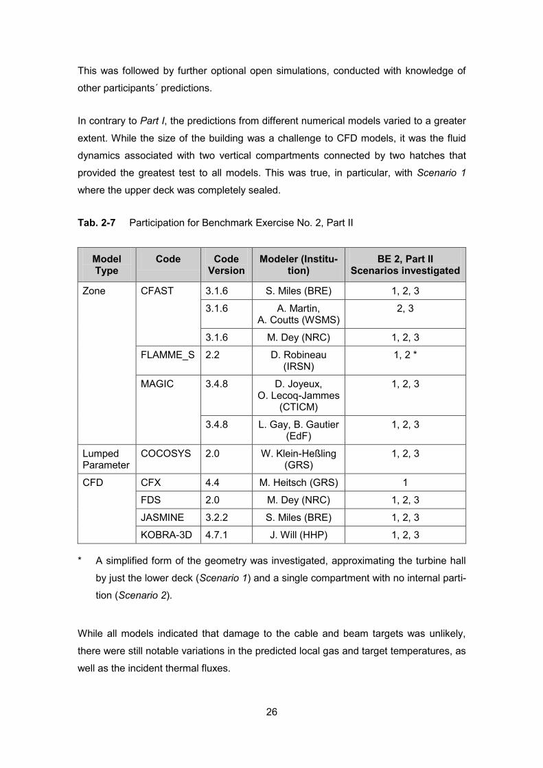
This was followed by further optional open simulations, conducted with knowledge of

other participants´ predictions.

In contrary to Part I, the predictions from different numerical models varied to a greater

extent. While the size of the building was a challenge to CFD models, it was the fluid

dynamics associated with two vertical compartments connected by two hatches that

provided the greatest test to all models. This was true, in particular, with Scenario 1

where the upper deck was completely sealed.

Tab. 2-7 Participation for Benchmark Exercise No. 2, Part II

Model Type

Code Code Version


BE 2, Part II Scenarios investigated

Zone CFAST 3.1.6 S. Miles (BRE) 1, 2, 3

3.1.6 A. Martin, A. Coutts (WSMS)

2, 3

3.1.6 M. Dey (NRC) 1, 2, 3

FLAMME_S 2.2 D. Robineau (IRSN)

1, 2 *


(CTICM)

1, 2, 3

3.4.8 L. Gay, B. Gautier (EdF)

1, 2, 3

Lumped Parameter


1, 2, 3

CFD CFX 4.4 M. Heitsch (GRS) 1

FDS 2.0 M. Dey (NRC) 1, 2, 3

JASMINE 3.2.2 S. Miles (BRE) 1, 2, 3

KOBRA-3D 4.7.1 J. Will (HHP) 1, 2, 3

* A simplified form of the geometry was investigated, approximating the turbine hall

by just the lower deck (Scenario 1) and a single compartment with no internal parti-

tion (Scenario 2).

While all models indicated that damage to the cable and beam targets was unlikely,

there were still notable variations in the predicted local gas and target temperatures, as

well as the incident thermal fluxes.

27

Fig. 2-12 illustrates inter-code predictions for upper and lower deck temperature condi-

tions for Scenario 2 (natural ventilation). Here, for the zone models the upper gas layer

temperature is plotted, and for the CFD and lumped parameter models the average gas

temperatures 1 m below the ceiling at thermocouple tree locations T1 and T2 are giv-

en. The rationale for selecting these measurement locations is that they are repre-

sentative of locations where a fire model might be employed to predict the thermal ha-

zard to a target such as a cable, and furthermore provide a ‘measure’ comparable to

the hot gas layer temperature in a zone model. While the results show that the different

fire models capture the same qualitative behavior, the ‘hot layer temperature rise’ [ºC]

does vary by up a factor of about two in both decks.

Fig. 2-13, however, illustrates that while there is broad agreement for the ‘hot layer

temperature rise’ in the lower deck for Scenario 1, there is a notable spread of values

for the upper deck where the predicted gas temperature rise varies by a factor of about

5 for the different fire models.

28

Part II Scenario 2 - upper deck hot layer temperature

0

20

40

60

80

100

120

0 120 240 360 480 600 720 840 960 1080 1200Time (s)

Tem

pera

ture

(C)

CFAST - BRECFAST - NRCCFAST - WSMSMAGIC - EDFMAGIC - CTICMCOCOSYSFDSJASMINEKobra3D - HHP

Part II Scenario 2 - lower deck hot layer temperature

0

50

100

150

200

250

300

0 120 240 360 480 600 720 840 960 1080 1200Time (s)

Tem

pera

ture

(C)

CFAST - BRECFAST - NRCCFAST - WSMSMAGIC - EDFMAGIC - CTICMCOCOSYSFDSJASMINEKobra3D - HHP

Note: Zone models (CFAST and MAGIC) - upper layer temperature plotted; lumped parameter and CFD models (COCOSYS, FDS, JASMINE and KOBRA-3D) - average of 'ceiling level' thermocouple tree locations at T1 and T2 plotted

Fig. 2-12 Inter-code comparison of 'hot layer' temperatures for Benchmark Exercise

No. 2, Part II, Scenario 2

29

Part II Scenario 1 - upper deck hot layer temperature

0

50

100

150

200

250

0 120 240 360 480 600 720 840 960 1080 1200

Time (s)

Tem

pera

ture

(C)

CFAST - BRECFAST - NRCMAGIC - EDFMAGIC - CTICMCOCOSYSFDSJASMINECFX4 - GRSKobra3D - HHP

Part II Scenario 1 - lower deck hot layer temperature

0

50

100

150

200

250

300

0 120 240 360 480 600 720 840 960 1080 1200Time (s)

Tem

pera

ture

(C)

CFAST - BRECFAST - NRCMAGIC - EDFMAGIC - CTICMCOCOSYSFDSJASMINECFX4 - GRSKobra3D - HHP

Note: Zone models (CFAST and MAGIC) - upper layer temperature plotted; lumped parameter and CFD models (COCOSYS, FDS, JASMINE and KOBRA-3D) - average of 'ceiling level' thermocouple tree locations at T1 and T2 plotted

Fig. 2-13 Inter-code comparison of 'hot layer' temperatures for Benchmark Exercise

No. 2, Part II, Scenario 1

30

2.2.4 Discussion

Part I

The results for Part I were judged encouraging, with the general, qualitative, nature of

the experiments being captured in the simulations by zone, lumped parameter and

CFD models. Comparison between predictions and measurements was restricted to

gas temperatures at three thermocouple trees and two locations directly above the fire

source. However, this was sufficient to allow the above issues to be addressed with

some degree of confidence.

The main findings are now summarized:

• Despite the ‘complexity’ of the roof structure the various types of model were able

to predict the smoke layer formation process with reasonable reliability. Of particu-

lar note here was the ability of zone models to make an assumption of a flat ceiling

such that the volume of the hall was conserved.

• Zone models generally predicted lower layer heights than those derived from the

experimental measurements using the suggested data reduction formula. This

might possibly be attributed to the flat ceiling approximation. An alternative expla-

nation may lie in the data reduction formula, where closer examination of the nu-

merical reduction method suggests that the layer height could be interpreted as be-

ing lower than the method suggests, especially later in the fire as illustrated in Fig.

2-14.

• For Scenario 1 and 2 the precise specification of the ’infiltration’ ventilation was not

important in respect to the predicted temperatures inside the test hall. This pro-

vides some encouragement in modeling such scenarios.

• When using the original Benchmark specification there was, in most cases, a ten-

dency to predict higher smoke layer temperatures than those measured. Two prin-

ciple mechanisms were identified, to which modifications were possible to reduce

the temperature of the smoke layer .

31

The first of these was the proportion of heat attributed to the convective power of

the fire plume, the value being dependent on the choice of heat of combustion,

combustion efficiency and radiative fraction. It seems that the choice of 80% for the

combined effect of combustion efficiency and radiative fraction was not ideal,

resulting in too much heat being convected into the upper layer. This may have

contributed to the predicted temperatures being higher than those measured.

The second was the boundary heat loss, which was shown to play an important

role in a number of studies.

Fig. 2-14 Measured temperature profiles and numerically reduced two-layer interface

for Benchmark Exercise No. 2, Part I, Scenario 1

Part II

A detailed, comparative analysis of the range of predicted maximum hazard levels pre-

sented inside the two decks, and also to the individual targets, was performed and is

presented in the Benchmark Exercise No. 2 Panel Report /MIL 04/. The main aspects

of this are reported below.

Measured temperatures at 300 s

02468

1012141618

0 10 20 30 40 50 60 70

Temperature rise (C)

Hei

ght (

m)

tree 1tree 2tree 3layer interface

Layer descending to floor?

Or possible radiative heating of thermo-couples?

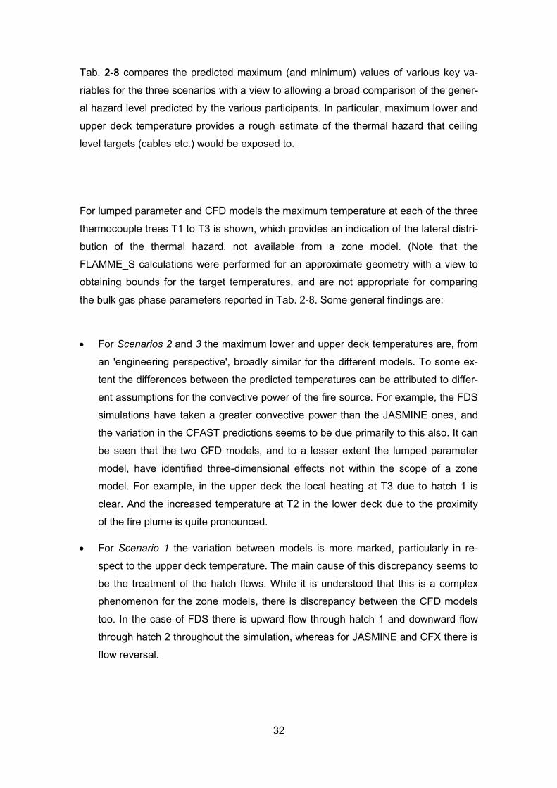
32

Tab. 2-8 compares the predicted maximum (and minimum) values of various key va-

riables for the three scenarios with a view to allowing a broad comparison of the gener-

al hazard level predicted by the various participants. In particular, maximum lower and

upper deck temperature provides a rough estimate of the thermal hazard that ceiling

level targets (cables etc.) would be exposed to.

For lumped parameter and CFD models the maximum temperature at each of the three

thermocouple trees T1 to T3 is shown, which provides an indication of the lateral distri-

bution of the thermal hazard, not available from a zone model. (Note that the

FLAMME_S calculations were performed for an approximate geometry with a view to

obtaining bounds for the target temperatures, and are not appropriate for comparing

the bulk gas phase parameters reported in Tab. 2-8. Some general findings are:

• For Scenarios 2 and 3 the maximum lower and upper deck temperatures are, from

an 'engineering perspective', broadly similar for the different models. To some ex-

tent the differences between the predicted temperatures can be attributed to differ-

ent assumptions for the convective power of the fire source. For example, the FDS

simulations have taken a greater convective power than the JASMINE ones, and

the variation in the CFAST predictions seems to be due primarily to this also. It can

be seen that the two CFD models, and to a lesser extent the lumped parameter

model, have identified three-dimensional effects not within the scope of a zone

model. For example, in the upper deck the local heating at T3 due to hatch 1 is

clear. And the increased temperature at T2 in the lower deck due to the proximity

of the fire plume is quite pronounced.

• For Scenario 1 the variation between models is more marked, particularly in re-

spect to the upper deck temperature. The main cause of this discrepancy seems to

be the treatment of the hatch flows. While it is understood that this is a complex

phenomenon for the zone models, there is discrepancy between the CFD models

too. In the case of FDS there is upward flow through hatch 1 and downward flow

through hatch 2 throughout the simulation, whereas for JASMINE and CFX there is

flow reversal.

33

• There is some discrepancy between models in terms of the relative level of thermal

hazard predicted for the different cases. For example, the MAGIC simulations indi-

cate that the smoke layer in Scenario 2 and 3 is markably hotter compared to Sce-

nario 1, whereas for FDS the reverse is true.

• The CFD models have predicted higher maximum plume temperatures than the

lumped parameter and zone models. This is most likely a consequence, in part at

least, of the fact that the CFD models have resolved the plume structure, and will

hence have identified the 'hot region'.

• In terms of the pressure and oxygen consumption predictions, the difference be-

tween the results is judged to be not that significant. Here is should be noted that a

small variation in 'leakage ventilation' rates can give rise to large differences in

compartment pressures, thus the difference between, approximately 500 and

1000 Pa may be not significant.

34

Tab. 2-8 Comparison of gas phase predictions for Benchmark Exercise No. 2, Part II

Scenario Property Zone Models CFD and Lumped Parameter Models

1

Maximum gas temperature in

lower deck (outside plume)

[°C]

T T1 T2 T3

CFAST (BRE)

CFAST (NRC)

MAGIC (EDF)

MAGIC

192 229 233 233 (CTICM)

JASMINE (BRE)

FDS (NRC) CFX-4 (GRS) 5

COCOSYS (GRS)

KOBRA-3D

216 230

194 390 (HHP)

249 278 238 244 385

217 371

234 354

1


upper deck [°C]

T T1 T2 T3

CFAST (BRE)

CFAST (NRC)

MAGIC (EDF)

MAGIC

90 98 56 56 (CTICM)

JASMINE (BRE) FDS (NRC)

CFX-4 (GRS)

COCOSYS (GRS) Kobra-3D

61 191

130 240 (HHP)

77 230 64

160 243

262 346 134 177 342

1

Maximum plume

temperature [°C]

6

T T

MAGIC (EDF)

MAGIC 461 460 (CTICM)

JASMINE (BRE) FDS (NRC)

COCOSYS

963 887 463 (GRS)

1

Maximum (net) heat convected

through hatches [MW]

T T

MAGIC 5 (EDF) JASMINE (BRE) FDS (NRC) COCOSYS

9 9

16 (GRS)

1

Maximum heat lost to solid boundaries

[MW]

T T

JASMINE (BRE) COCOSYS

40 37 (GRS)

1

Maximum relative static

pressure [Pa]

T T

CFAST (BRE) CFAST (NRC) MAGIC (EDF) MAGIC

599 698

1280 1278 (CTICM)

JASMINE (BRE) FDS (NRC) CFX-4 (GRS) 5 COCOSYS

475 1367 1051 1580 (GRS)

1 Minimum O2

concentration [%]

T T

CFAST (BRE) CFAST (NRC)

MAGIC (EDF)

MAGIC

15.9

(CTICM)

1

13.61

12.11

12.2

JASMINE

1

(BRE)

FDS (NRC)

CFX-4 (GRS) 5

COCOSYS

13.6

(GRS)

2

11.81

15.01

16.2

1

2


lower deck (outside plume)

[°C]

T T1 T2 T3

CFAST (BRE) CFAST (NRC) CFAST (WSMS) MAGIC (EDF) MAGIC

194 252

215

(CTICM)

3/2434

JASMINE

195 193

(BRE)

FDS (NRC)

COCOSYS (GRS) Kobra-3D

148 191 129 132 (HHP)

157 236 157 130

104 167 152 64

2


upper deck [°C]

T T1 T2 T3

CFAST (BRE) CFAST (NRC)

68 88

JASMINE (BRE) FDS (NRC) 58

72 61 80

120163

35

Scenario Property Zone Models CFD and Lumped Parameter Models

CFAST (WSMS) MAGIC (EDF) MAGIC

96

(CTICM)

3/1224 COCOSYS 105 95

(GRS) Kobra-3D

99 65

(HHP)

120 64

128 90

2

Maximum plume

temperature [°C]

6

T T1 T2 T3

MAGIC (EDF) MAGIC

244 238 (CTICM)

JASMINE (BRE) FDS (NRC) COCOSYS

947 791 279

(GRS)

2

Maximum (net) heat convected


T T1 T2 T3


37 46 37

(GRS)

2

Maximum heat lost to solid boundaries

[MW]

T T1 T2 T3

JASMINE (BRE) COCOSYS

18 22

(GRS)

3


lower deck (outside

plume) [°C]

T T1 T2 T3

CFAST (BRE) CFAST (NRC) CFAST (W'SMS) MAGIC (EDF) MAGIC

196 266

216

(CTICM)

3/2384

JASMINE

195 195

(BRE) FDS (NRC) COCOSYS (GRS) Kobra-3D

147 197 128 329

(HHP)

164 241 155 315

113 172 150 219

3


upper deck [°C]

T T1 T2 T3

CFAST (BRE) CFAST (NRC) CFAST (WSMS)

MAGIC (EDF) MAGIC

94 139

98

(CTICM)

3/1324

JASMINE

100 98

(BRE) FDS (NRC) COCOSYS (GRS) Kobra-3D

82 105 101

(HHP)

91 120 119

137 175 128

3 Maximum

plume tem-perature [°C]

6

T T1 T2 T3

MAGIC(EDF) MAGIC

245 248 (CTICM)

JASMINE (BRE) FDS (NRC) COCOSYS

986 820 277 (GRS)

3

Maximum heat convected


T T1 T2 T3


31 44 37 (GRS

3

Maximum heat lost to

solid boundaries

[MW]

T T1 T2 T3

JASMINE (BRE) COCOSYS (GRS) 27

22

1 volume % 2 mass % 3 rad fraction = 0.51 4 rad fraction = 0.2 5 first 864 s 6 8 m above fire for CFD

36

The Benchmark Exercise No. 2 Panel Report /MIL 04/ includes detailed comparisons

for the peak hazard conditions at the targets. In the case of zone models, the maximum

gas temperature at the targets corresponds to the temperature in the layer in which the

target is located.

While the general consensus was that cable and beam target damage would not have

occurred, the level of thermal hazard posed was quite varied between the different

models. This was a consequence of the variation in gas phase conditions, and also the

modeling of the incident flux. The flux predictions, in particular, were in some instances

quite varied, which will have directly influenced the predicted surface and centre-line

target temperatures.

The JASMINE simulations indicated fairly severe conditions for beam 1 due to its prox-

imity to the fire source, with high local gas temperature and incident flux levels, and

provided conditions closest to those indicating damage. For the models that provided

surface and center-line temperature predictions the agreement was in some instances

quite close, and in others more varied. Of particular note was the variation in some of

the target temperatures predicted in the two MAGIC contributions. The variation in pre-

dicted conditions at the human target was quite significant too. In the case of zone

models this can be explained, in part, by whether the human target was located in the

upper or lower layer.

Overall, it seems clear that further 'validation' of existing fire models is required for the

type of scenario represented by Part II. Comparison against measurements would be

useful here. Issues identified for further work are included in the Conclusions section

below.

2.2.5 Conclusions

Benchmark Exercise No. 2 provided some valuable insights into the performance of fire

models, extending the findings from the first Benchmark Exercise in a number of impor-

tant respects. These included the modeling of large spaces, complex geometries and in

comparing predictions against experimental measurement data. Confidence in the ap-

plication of zone, lumped parameter and CFD models has been provided in the simula-

tions of the test hall experiments in Part I, where reasonable agreement was obtained

once the important, controlling mechanisms were accounted for.

37

However, the simulations of the hypothetical turbine hall in Part II identified a number of

current weaknesses, and illustrated that quite varied predictions could be obtained with

different models, including with those of the same type, e.g. zone or CFD models.

Despite the 'complexity' of the roof structure in Part I the various models were able to

predict the smoke layer formation process with reasonable reliability. Of particular note

here was the justification in assuming a flat ceiling with the zone models, with the

height set such that the volume of the hall was conserved. The fact that zone models

generally predicted lower layer heights than those derived from the experimental mea-

surements might be attributed, in part at least, to the data reduction method used in

calculating the layer height from the experimental temperature measurements.

When using the original Benchmark specification, there was a tendency in Part I to

predict higher smoke layer temperatures than those measured. Two principle mechan-

isms were identified, to which modifications were able to reduce the temperature of the

smoke layer. The first of these was the proportion of heat attributed to the convective

power of the fire plume, the value being dependent on the choice of heat of combus-

tion, combustion efficiency and radiative fraction. The second was the boundary heat

loss, which was shown to play an important role in a number of studies.

In contrary to Part I, the predictions form different numerical models for Part II varied to

a greater extent. This is perhaps not surprising given the complexity of the fluid dynam-

ics and the fact that measurements were not available against which to compare simu-

lations. While the size of the building was a challenge to CFD models, it was the fluid

dynamics associated with two vertical compartments connected by two hatches that

provided the greatest test to all models. This was true, in particular, to Scenario 1

where the upper deck was completely sealed.

For Scenarios 2 and 3, the maximum lower and upper deck temperatures were, from

an 'engineering perspective', broadly similar for the different models. To some extent

the differences between the predicted temperatures could be attributed to the different

assumptions for the convective power of the fire source. It was apparent that the CFD

models, and to a lesser extent the lumped parameter model, identified three-

dimensional effects not within the scope of a zone model.

38

For Scenario 1 the variation between models was more marked, in particular in respect

to the upper deck temperature. The main cause of this discrepancy seems to be the

treatment of the hatch flows. This is known to be a complex phenomenon for the zone

models, both for single vent and multiple vent scenarios. However, there were discre-

pancies between the CFD models, too, with differences in the predicted hatch flow me-

chanisms. Further development and validation in respect to the ability of all types of fire

models to predict flows through horizontal hatch type openings seems to be required.

By contrast, in terms of the pressure and oxygen consumption predictions, the differ-

ence between the various models was judged not to be significant.

While the general consensus was that cable and beam target damage would not have

occurred, the predicted level of thermal hazard varied quite significantly between differ-

ent models. This was a consequence of differences in gas phase conditions and also

the modeling of the incident flux. The flux predictions, in particular, were in some in-

stances quite varied, which will have directly influenced the surface and centre-line

target temperatures for those models including these calculations.

As in the first Benchmark Exercise, the treatment of the radiative fraction and effective

heat of combustion had a big influence on the results. The difference in the predicted

temperatures for the various models in Part II, and discrepancies with measurements in

Part I, seems to have been due, in part at least, to assumptions made here.

Further development of suitable sub-models for predicting the thermal damage to tar-

get elements, in particular cables, cable bundles and cable trays, seems to be required.

The calculation of incident fluxes is particularly important in predicting cable damage,

and highlights the need to address the radiative heat transfer, both from the flaming

region and the smoke layer, more carefully.

The usefulness in applying a combination of simpler (e.g. zone) and more complex

(e.g. CFD) models to practical problems akin to those represented by the Benchmark

Exercise was apparent. In particular, the zone model approach, while obviously more

limited in its geometrical and scientific capabilities, provides a very useful tool for an

initial scoping study. CFD can then be used for selected scenarios as required in a par-

ticular safety study. This may be particularly important for large geometries such as a

turbine hall where CFD calculations are likely to be expensive.

39



The design of Benchmark Exercise No. 3 incorporated several lessons learned from

previous NRC-sponsored large scale fire tests. Most importantly, a considerable em-

phasis was placed on obtaining material properties (cables, in particular), ventilation

flow rates, leakage rates, and enough measurements to estimate the integrated heat

losses through the walls and compartment opening. This information is vital for a model

validation exercise.


The experiments for Benchmark Exercise No. 3 were designed by staff members from

the U.S. NRC and NIST. A draft specification of the experiments was issued to partici-

pants on September 6, 2002, to solicit comments, further ideas, and suggestions. Writ-

ten comments on the draft specification were received from participants.

Benchmark Exercise No. 3 consisted of 15 large scale experiments performed at NIST in

June 2003. Numerous measurements (350 per test) were made including gas and sur-

face temperatures, heat fluxes and gas velocities. The experiments are documented in

/HAM 06/. Only a brief description of the experiments is included here.

The test compartment dimensions were 21.7 m x 7.1 m x 3.8 m high. The walls and ceil-

ing were lined with two layers of marinate boards; the floor was covered with one layer

of gypsum board on top of one layer of plywood. Thermo-physical properties of the ma-

rinite and other materials were provided to the participants. The compartment had one 2

m by 2 m door and a mechanical air injection and extraction system. Some of the tests

were conducted with the door closed and no mechanical ventilation, and in those tests

the measured compartment leakage was an important consideration. /HAM 06/ reports

leakage areas based on measurements performed prior to five of the fifteen tests.

Ventilation conditions, the fire size, and fire location were the key parameters varied in

the test series. The fire pan was located at floor level in the center of the compartment

for most of the tests. In three tests, the fire was positioned near the wall.

40

The fuel pan was 2 m long, 1 m wide and 0.1 m deep. The fuel used in 14 of the tests

was heptane, while toluene was used for one test. The heat release rate was deter-

mined using both the estimated fuel flow rate and oxygen consumption calorimetry.

The uncertainty in the HRR measurement is described in /HAM 06/. The recommended

uncertainty values were 17 % for all of the tests.

The photograph presented in Fig. 2-15 shows a typical benchamerk Exercise No. 3

experiment. A heptane spray fire can be observed through the open doorway, which

was instrumented to measure the temperature and velocity fields.

Fig. 2-15 Photograph of a Benchmark Exercise No. 3 experiment conducted in a

large compartment at NIST

41

2.3.3 Results

It is difficult to summarize in a simple way the accuracy of the models assessed in

Benchmark Exercise No. 3, as each participant chose different quantities and different

tests to analyze, see Tab. 2-9. Some performed calculations before the test data was

released (blind calculations), some after (open calculations). Some used the recom-

mended values of the input parameters; others chose to vary the parameters to assess

sensitivity. All of the participants agreed that the approximate forms of the conservation

equations for mass, momentum and energy in the various fire models evaluated pro-

vide a ‘reasonable’ prediction of the hot gas layer temperature, depth and product con-

centration. Other issues were discussed on a case by case basis. Tab. 2-10 presents a

sample of the qualitative assessments. All of the participants considered the influence

of the HRR, leakage rate, ventilation rate, door opening and material properties, but in

a very qualitative way. For example, a higher specified radiative fraction leads to lower

upper layer temperatures. Splitting the ventilation duct between the upper and lower

layers of a zone model influenced the layer height.

Tab. 2-9 Models used for Benchmark Exercise No. 3

Model Type

Code Code Version


Blind (b), Semi-blind (s) or Open (o) Calcula-

tion

Zone CFAST 3.1.6 S. Miles (BRE) b, s

3.1.7 M. Dey (Deytec) s, o

FATE 2.0 T. Elicson, S.J. Lee, M. Plys

(Fauske)

o

FLAMME_S 2.3.2 L. Rigollet (IRSN) s

MAGIC 3.4.8 L. Gay, B. Gautier (EdF)

b, s

Lumped Parameter


b, s, o

CFD CFX 5.7 M. Heitsch (GRS) s

FDS 4.0 K. McGrattan (NIST)

s

4.0.5 M. Dey (Deytec) s, o

JASMINE 3.2.3 S. Miles (BRE) b, s

42

Tab.

2-1

0 I

ndiv

idua

l Ass

essm

ents

of M

odel

Acc

urac

y, B

ench

mar

k Ex

erci

se N

o. 3

C

FAST

S.

Mile

s (B

RE)

FATE

M

. Ply

s (F

ausk

e)

FLAM

MM

E_S

L. R

igol

let

(IRSN

)

MAG

IC

L G

ay

(EdF

)

CO

CO

SYS

W. K

lein

-H

eßlin

g (G

RS)

CFX

M

. Hei

tsch

(G

RS)

FDS

K. M

cGra

ttan

(NIS

T)

JASM

INE

S. M

iles

(BR

E)

HG

L te

mpe

ra-

ture

“goo

d ag

reem

ent”

“s

imul

ated

ade

-qu

atel

y”

"goo

d, le

ss

than

12

%”

“qui

te g

ood”

; op

en “b

ette

r”

than

blin

d

case

by

case

“1

0 %

with

ex

cept

ions

” “a

ccur

atel

y ca

ptur

ed”

HG

L de

pth

“goo

d”

“flow

-sp

littin

g”

impo

rtant

good

agr

eem

ent”

“qui

te g

ood,

le

ss th

an

20 %

”

ca

se b

y ca

se

not a

sses

sed

“app

rox-

imat

ely

…

corr

ect”

Gas

es

“rea

sona

ble”

“goo

d re

sults

” ca

se b

y ca

se

case

by

case

ca

se b

y ca

se

“10

% in

mos

t ca

ses”

“r

easo

nabl

e”

Pres

sure

se

nsiti

ve to

le

akag

e le

akag

e im

-po

rtant

“g

ood

agre

emen

t” ca

se b

y ca

se

case

by

case

“with

in e

xp.

unce

rtain

ty”

sens

itive

to

leak

age

Hea

t flu

x “q

uite

var

ia-

ble”

“v

alid

ated

” “w

ell p

redi

cted

” ca

se b

y ca

se

case

by

case

“te

ndin

g to

ov

er-p

redi

ct”

Targ

et

tem

pera

-tu

res

“rea

sona

ble”

“e

ffect

ive

cabl

e m

odel

” se

nsiti

ve to

doo

r op

enin

g ca

se b

y ca

se

case

by

case

10 %

to 2

0 %

“r

easo

nabl

e”

“rea

sona

ble”

Doo

r flo

ws

“goo

d ag

reem

ent”

ov

er-p

redi

cted

ne

ar s

ill

“cap

ture

d ac

cura

tely

”

Ove

rall

“enc

oura

g-in

g”

“enc

oura

ging

” “q

uite

goo

d”

“wor

se” t

han

othe

r Ben

ch-

mar

k Ex

erci

s-es

“suf

ficie

ntly

ac

cura

te”

“enc

oura

g-in

g”

43

2.3.4 Discussion

Benchmark Exercise No. 3 consisted of 15 experiments, each of which consisted of

350 point measurements. With little or no guidelines for analysis, the participants chose

to assess their models as they saw fit. The individual reports consist of dozens of ob-

servations, but little quantification of model accuracy. Most fire modeling analyses pub-

lished over the past 30 years have a similar character.

However, some regulatory authorities like the U.S. NRC, and standards bodies in the

U.S. like the National Fire Protection Association (NFPA), are meanwhile demanding a

more quantitative assessment of fire model accuracy. Given the adoption of NFPA 805

/NFP 01/, the U.S. NRC now requires that all fire models used for NPP safety assess-

ment be verified and validated (V&V). Towards this end, the U.S. NRC has more re-

cently published a seven-volume report, ‘Verification and Validation of Selected Fire

Models for Nuclear Power Plant Applications’ /NRC 07/ being available to the public on

the NRC’s Web site1

1

. Five of the seven volumes contain individual evaluations of fire

models having also been applied in the frame of ICFMP Benchmark ExerciseNo. 3

such as CFAST, MAGIC, FDS. Fifteen of the 26 experiments used for the NRC V&V

study /NRC 07/ are from Benchmark Exercise No. 3. Results from Benchmark Exercis-

es No. 2, 4 and 5 were also used, as were two sets of experiments performed at the

National Bureau of Standards (now NIST) and Factory Mutual (under sponsorship of

the NRC).

A key component of /NRC 07/ is the quantification of experimental uncertainty. In fact,

the final assessments for all the models considered were made in light of the experi-

mental uncertainty for the quantities that were being compared. An example of the

process to determine experimental uncertainty is as follows; suppose that the uncer-

tainty in the measurement of the heat release rate of a fire was determined to be 15 %.

According to the well known McCaffrey, Quintiere, Harkleroad (MQH) correlation, the

upper layer gas temperature rise in a compartment fire is proportional to the two-thirds

power of the heat release rate. This means that the 15 % uncertainty in the measured

heat release rate that is input into the fire models leads to a 10 % uncertainty in the

prediction of the upper layer temperature.

www.nrc.gov/reading-rm/doc-collections/nuregs/staff/

http://www.nrc.gov/reading-rm/doc-collections/nuregs/staff/�

44

Combining this with the uncertainty associated with the thermocouple temperature

measurement leads to a combined uncertainty in the reported temperature of about

12 %.

This type of analysis is particularly important for Benchmark Exercise No. 3. The origi-

nally specified heat release rate (HRR) for most of the Benchmark Exercise No. 3 ex-

periments was 1 MW. This was the HRR used in the blind exercise. However, after the

experiments were completed, the HRR was reported to be on the order of 1.15 MW,

15 % higher than the original estimate. To put this into perspective, consider the set of

graphs shown in Fig. 2-16, Tests 2, 3 and 4 (the original blind simulation cases) were

re-run with the CFD model FDS using different HRR values of 1000 kW, 1150 kW, and

1190 kW.

Notice that the heat release rate has little effect on the hot gas layer height predictions,

but it does have a noticeable effect on the hot gas layer temperature predictions. The

difference between the 1150 kW and 1190 kW simulations is fairly small, and well with-

in the uncertainty bounds of the HRR measurement itself. However, the 1000 kW simu-

lations noticeably under-predict the HGL temperature. This is not surprising, because

the HGL temperature rise is proportional to the two-thirds power of the HRR, according

to the well-established MQH correlation. Thus, a 15 % change in the input heat release

rate will yield a 10 % change in the hot gas layer temperature rise.

45

Hot Gas Layer TemperatureICFMP BE #3, Test 2

Time (min)

0 5 10 15 20 25 30

Tem

pera

ture

(C)

0

50

100

150

200

250

300

ExperimentFDS (1190 kW Fire)FDS (1140 kW Fire)FDS (1000 kW Fire)

Hot Gas Layer HeightICFMP BE #3, Test 2

Time (min)

0 5 10 15 20 25 30

Hei

ght (

m)

0

1

2

3

4



Time (min)

0 5 10 15 20 25 30

Tem

pera

ture

(C)

0

50

100

150

200

250

300



Time (min)

0 5 10 15 20 25 30

Hei

ght (

m)

0

1

2

3

4



Time (min)

0 5 10 15 20 25 30

Tem

pera

ture

(C)

0

50

100

150

200

250

300



Time (min)

0 5 10 15 20 25 30

Hei

ght (

m)

0

1

2

3

4


Fig. 2-16 Measured and predicted hot gas layer temperature and height for Bench-

mark Exercise No. 3, Tests 2, 3 and 4

46

A similar analysis was performed for the other quantities of interest. In Volume 2 of

/NRC 07/, Hamins quantifies the experimental uncertainty of Benchmark Exercise

No. 3 (see Tab. 2-11). Experimental uncertainty is due to both uncertainty in the mea-

surements of the model input parameters (such as the heat release rate), and also the

measurement of the model output quantities (such as the gas temperature). By quanti-

fying the experimental uncertainty, especially the consequence of uncertainty in model

inputs, it becomes much easier to re-assess the qualitative conclusions drawn by the

participants of Benchmark Exercise No. 3.

All the participants noted how sensitive their results were to leakage and ventilation

rates. Some went so far as to say that their models were performing badly based on

the apparent discrepancy between their predicted pressures and the measured pres-

sures. However, consider that the uncertainty in the specified leakage and ventilation

rates can lead to as much as an 80 % combined uncertainty in the reported measure-

ments. In other words, any model within 80 % of the measured pressure could claim to

be within experimental uncertainty, and no further assessment can be made, based on

this set of experimental data.

The real value of Hamins’ uncertainty analysis is that it quantifies what has been re-

ferred to as ‘User Effects’ by the ICFMP participants. All the participants pointed to the

HRR, leakage rate, and ventilation rate as key parameters, and now we see why. The

compartment pressure, for example, goes like the square of each. However, the hot

gas layer depth was well-predicted by all because it is not sensitive to input parameters

that have a high degree of uncertainty. For any fire scenario, there are dozens of input

parameters that a modeler must specify. A simple uncertainty analysis like the one de-

scribed here will focus attention on those inputs that really matter.

The above discussion quantifies the sensitivity of model results to model inputs. But it

does not tell us how accurate the models are. To assess accuracy, there first must be a

standard metric to quantify the difference between the measurement and the model

prediction. For Benchmark Exercise No. 3, there was no single metric that the partici-

pants used to quantify the accuracy of each point to point comparison. However, in

/NRC 07/, a relative difference was defined as the difference between the peak value of

the prediction and the peak value of the measurement, divided by the peak value of the

measurement. This definition was specified by the regulatory authority because peak

values are seen as a good measure of the severity of the fire.

47

Tab. 2-11 Sensitivity of model outputs from /NRC 07/

Quantity Important Input Pa-rameters

Power Depen-dence

Combined Uncertainty [%]

HGL tempera-ture HRR

Fehler! Text-marke nicht definiert.

12 2/3

HGL depth door height TC spacing

1 1 63

Gas concentra-tions HRR 1/2 9

Smoke concen-tration

HRR soot yield

1 1 33

Pressure HRR

leakage rate vent rate

2 2 2

40 (unventilated) 80 (ventilated)

Heat flux HRR 4/3 20

Surface/Target temperature HRR 2/3 14

Once all of the relative differences for all of the chosen quantities had been calculated,

the results were assembled into simple scatter plots. These scatter plots provided a

very effective way to compare models, and types of models. Consider, for example, the

predicted average hot gas layer temperature rise (determined using a simple two layer

reduction method) from all the models compared to the experimental measurements as

shown in Fig. 2-17.

The data shown there are from Benchmark Exercises No. 2, 3, 4 and 5, plus several

other NRC and NIST sponsored experiments. The combined experimental uncertainty

of 13 % is an average for all the data sets. For Benchmark Exercise No. 3 alone, the

uncertainty was estimated at 12 %. The hand calculation methods show the greatest

deviation and scatter when compared to the measurements. Both the zone and CFD

models show less scatter and very similar accuracy for the experiments under consid-

eration.

48

Measured HGL Temperature Rise (°C)

0 100 200 300 400

Pred

icted

HGL

Tem

pera

ture

Rise

(°C)

0

100

200

300

400

CFD ModelZone ModelsHand Calculation Methods

+13 %

-13 %

Fig. 2-17 Measured versus predicted hot gas layer temperature rise from different

ICFMP Benchmark Exercises and other experiments (from /NRC 07/)

Next, consider the predicted heat fluxes onto various horizontally and vertically oriented

targets in Fig. 2-18.

The CFD model, overall, is more accurate for this parameter, even though the zone

and CFD models are of comparable accuracy in predicting the gas temperature. Why is

the CFD model more accurate in predicting heat flux? The heat flux at a target is de-

pendent on the thermal environment of the surroundings, the details of which the CFD

model is inherently better able to predict. Hand calculations and zone models predict

average temperatures over the entire compartment, and thus are less accurate in pre-

dicting a heat flux to a single point.

Whereas the CFD model was more accurate in predicting heat fluxes and surface tem-

peratures, the simpler models performed equally well, sometimes better, for plume and

ceiling jet temperatures and flame heights. The reason is that hand calculations as well

as simple zone models with only a hot gas and a cold gas layer (two zones) use well-

established correlations for these fire phenomena.

49

A CFD model solves the basic transport equations, making it truly predictive of these

quantities, but not necessarily more accurate. And the increased cost of a CFD calcula-

tion is substantial. The spreadsheet and two-zone models produce results in seconds

to minutes, versus a CFD model which takes hours to days. If hand calculations and

zone model results are obtained faster and are equal to (or better than) CFD results,

why should an engineer use a CFD model. Real fire scenarios can be more complex

than the experiments used in this study and may not conform to the assumptions inhe-

rent in the hand calculations and zone models. Fire plumes may not be free and clear

of obstacles, because fires sometimes occur in cabinets or near walls. Ceilings might

not be flat and unobstructed, because duct work, structural steel, and cable trays are

often present. Although hand calculations and zone models can be applied in these

instances, the results require more extensive explanation and justification. Since CFD

models can make predictions on a more local level with fewer assumptions, the results

are likely to be more applicable in these more complex situations.

Measured Radiation Heat Flux (kW/m2)

0 2 4 6 8 10

Pred

icted

Rad

iation

Hea

t Flux

(kW

/m2 )

0

2

4

6

8

10

CFD ModelZone ModelsHand Calculation Methods

+20 %

-20 %

Fig. 2-18 Measured versus predicted radiation heat flux onto various horizontally and

vertically oriented targets in Benchmark Exercise No. 3 (from /NRC 07/)

50

2.3.5 Conclusions

Benchmark Exercise No. 3 provided a tremendous amount of experimental data with

which to assess fire models. The participants in this exercise used these data in vari-

ous ways, but without a common framework for analysis. Thus it was difficult to assess

the relative accuracies of the different models. However, the further analysis of the

ICFMP Benchmark Exercise No. 3 data that is included in /NRC 07/ should allow the

Benchmark Exercise No. 3 participants to re-evaluate their models in light of the quanti-

fying metrics developed. Although only five models were assessed in the above men-

tioned NRC/EPRI study /NRC 07/, the process provides a means to evaluate any fire

model in a consistent manner against a common database of experiments. The study

highlights the use of experimental uncertainty as a means to assess the level of

agreement between models and measurements. It also provides a way of quantifying

‘User Effects’.

Much remains to be done in improving fire models beyond the basic transport capabili-

ties that were assessed in Benchmark Exercise No. 3. But before any improvements

can be made, the accuracy of the commonly used models has to be quantified rigo-

rously, so that resources can be spent on the parts of the models that need the most

improvement. At this stage, the basic transport algorithms within the zone and CFD

models were shown to be robust and nearly comparable to the uncertainty of the mea-

surements against which they were compared. Heat flux and surface temperature pre-

dictions are more challenging and could benefit from continued development. Hand

calculations are typically less accurate than zone or CFD models, but are easy to use

and predictably conservative.

51


At iBMB (Institut für Baustoffe, Massivbau und Brandschutz) University of Braun-

schweig - Institute of Technology in Germany, a set of nine real scale fuel pool fire ex-

periments has been performed. The objective of these experiments was to systemati-

cally vary the major influencing parameters on the burning behavior to derive standard

fire curves (time dependence of temperatures and heat flow densities at different dis-

tances from the fire source, burning rates, energy release rates and temperature loads)

and to examine the dependence on the pool surface area, the fuel filling level and the

ventilation conditions. Test 1 and Test 3 have been used for the Benchmark Exercise

No. 4. Details of the specification and results are published in /KLE 06/.


The main objective of the experiments for Benchmark Exercise No. 4 was to analyze

the thermal load on the structures surrounding a fire relatively large compared to the

floor area and volume of the fire compartment. In several experiments the natural and

forced ventilation has been varied to investigate the influence of oxygen depleted con-

ditions on the fire. However, the thermal loads and the oxygen depleted conditions are

somewhat difficult aspects to calculate, and therefore these experiments can contribute

to the further improvement of fire codes. Additionally, the results give some insight

concerning the uncertainties of simulations of pool fires in an enclosure under the given

boundary conditions.


The fire compartment ‘OSKAR’ of iBMB, an enclosure with a compartment floor size of

3.6 m x 3.6 m = 12.96 m2

Fig. 2-19 and a height of 5.7 m, was used for the pool fire test series

(see ). The opening in the front (with different sizes in the Tests 1 and 3) was

open only for the natural ventilation of the fire compartment. Above the front door a

hood was placed to measure the gas composition of the smoke.

52

Inside the fire compartment the gas temperatures, wall surface temperatures, wall heat

fluxes and surface as well as the inner temperatures at the material probes (3 plates of

different materials and one barrel container, see Fig. 2-20), gas concentration and the

gas velocity at the front opening have been measured.

Fig. 2-19 3D view of the OSKAR fire compartment used for Benchmark Exercise

No. 4

53

Fig. 2-20 View of the three material probes implemented in the Benchmark Exercise

No. 4 test compartment

At the beginning of the experiments the pan was filled with fuel, with the chemical

summary formula C11.64H25.29

2.4.3 Results

. In all experiments the fuel level was 0.1 m. To ignite the

fuel pool, a cleaning rag soaked with liquid fuel was put at the corner of the pan. Then

the outer end was ignited, leading to ignition of the whole pool. The duration of this

process was approx. 30 to 60 s. The experiments ran until the fuel was consumed.

In those tests considered for Benchmark Exercise No. 4 the fan system was running.

Although the valves on the top of the fire compartment should have been closed, some

velocity was measured. Due to these measurements, some leakages from the ceiling

of the fire compartment have to be assumed.

In the following, the experimental results, and some main results of the fire simulations

performed will be discussed. The list of performed calculations is given in Tab. 2-12.

54

The FATE calculation is not presented, because no calculated data values are avail-

able. In cases where a participant has delivered several calculations then one of these

has been selected.

To obtain an overview of the calculated results a FFT (Fast Fourier Transformation)

based method (FFTBM) /LEO 94/ has been used to compare these results to the expe-

rimental data.

The differences based on the continuously varying error function ( ) ( ) ( )tFtFtF c exp−=∆ ,

continuously varying, should be condensed to give a limited number of values that

could be taken as indexes for quantifying accuracy. Integral approaches satisfy this re-

quirement, since they produce a single value on the basis of the instantaneous trend of

a given time function. On the other hand, care should be taken in expressing all the in-

formation through a single value to avoid the loss of significant details. A fundamental

property of the Fourier transformation is that the differences can be analyzed from a

different viewpoint without any lack of information with respect to the original one. The

accuracy quantification of a code calculation is based on the amplitude of the FFT of

the experimental signal and of the difference between experimental signal and the cal-

culated trend. In particular, the method characterizes each calculation through two val-

ues. Using the error function ( ) ( ) ( )tFtFtF expc −=∆ and the discrete Fourier transforma-

tions F~∆ and expF~ via FFT a dimensionless average amplitude

( )

( )∑

∑

=

=

∆= m

m

2

0nnexp

2

0nn

fF~

fF~

AA

and a weighted frequency

( )

( )∑

∑

=

=

⋅∆= m

m

2

0nnexp

2

0nnn

fF~

ffF~

WF

is defined.

55

The most significant information is given by the average amplitude AA, which

represents the relative magnitude of the discrepancy derived from the comparison be-

tween two curves. (AA = 1 means a calculation affected by a 100 % of error.) The

weighted frequency (WF) factor characterizes the kind of error, because its value em-

phasizes whether the error has more relevance at low or high frequencies. A larger

value of 1/WF (inverse of WF) indicates larger deviations for low frequencies. Depend-

ing on the transient, high frequency errors can be more acceptable than low frequency

ones. Depending on the transient, high frequency errors can be more acceptable than

low frequency ones. For receiving meaningful results it can be compared qualitatively.

Such a qualitative comparison is therefore needed before.

The above described FFTBM has been used within several ISP (International Standard

Problem) projects. Based on the experience gained /LEO 94/ (roughly 200 code calcu-

lations analyzed from about ten experiments), an upper limit of AAtot = 0.4 has been

chosen as reference threshold value identifying good accuracy of a code calculation.

AAtot is a weighted average value over all relevant data for the corresponding experi-

ment.

For this kind of comparison a few variables have been selected. These are the plume

temperature M3, the atmospheric gas temperatures at the second level at 3.35 m M11

to M14, the upper layer temperature Tup, the surface temperatures of the three material

probes M29, M33 and M34 and the oxygen concentration at position GA1. Only the

time period from 0 s to 800 s is considered for both tests, during which time the mea-

surement of the fuel weight loss is reliable.

56

Tab. 2-12 List of calculations performed for Benchmark Exercise No. 4

Model Type

Code Code Version

Modeler (Institution)

Part I Part II

Zone CFAST 3.1.6 CFABRs S. Miles (BRE)

semi-blind

semi-blind 1 2

3.1.7 CFANRs M. Dey (NRC/NIST)

semi-blind

semi-blind

FLAMME_S

2.3.2 FLAIRo L. Rigollet (IRSN)

open open 3 3

FATE 2.0 (not pre-sented)

T. Elicson (Fauske)

open open

MAGIC 4.1.1b MAGEDo B. Gautier (EdF)

open open

Lumped Parameter

COCOSYS 2.2dev COCGRo B. Schramm (GRS)

open open

CFD CFX 5 CFXGRo M. Heitsch (GRS)

open open

FDS 3.1.5 FDSNRs M. Dey (NRC/NIST)

semi-blind

semi-blind

3 FDSGRo W. Brücher (GRS)

open4

4 FDSNIb K. McGrattan (NIST)

blind blind

4 FDSNIs K. McGrattan (NIST)

semi-blind

semi-blind

JASMINE 3.2.3 JASBRb S. Miles (BRE)

blind blind 5 5

3.2.3 JASBRs S. Miles (BRE)

semi-blind

semi-blind 6

3.2.3 JASBRo S. Miles (BRE)

open 7

VULCAN VULSAo V. Nicolette (SNL)

open

1 CFAST 3.1.6 semi-blind calculation: run 1 with measured pyrolysis rate (see Table B1 in Appendix B of /KLE 06/) 2 CFAST 3.1.6 semi-blind calculation: run 3 with limited measured pyrolysis rate (see Table B1 in Appendix B of /KLE 06/) 3 FLAMME_S open calculation with measured pyrolysis rate (see Appendix E of /KLE 06/) 4 FDS 3 calculation using the coarse grid resolution (see Appendix G of /KLE 06/) 5 JASMINE 3.2.3 blind calculation: run1 with constant pyrolysis rate of 0.039 kg s-1 (see Table B2 in Appendix B of /KLE 06/) 6 JASMINE 3.2.3 semi-blind calculation: run1 with measured pyrolysis rate (see Table B3 in Appendix B of /KLE 06/) 7 JASMINE 3.2.3 open calculation: run4 with 0.75 x measured pyrolysis rate (see Table B4 in Appendix B of /KLE 06/)

57

Atmospheric Temperatures Inside the Fire Compartment

Fig. 2-21 and Fig. 2-22 present the FFT results for the atmospheric temperatures M3

(plume) and M11 to M14 (Level 2) for Test 1 and Test 3, respectively. The following

conclusions can be drawn:

− The simulation of the upper layer temperature in Test 1 is much worse than Test 3

for CFD calculations. It has to be kept in mind, that only three levels of temperature

measurements are available. Therefore the calculation of the experimental upper

layer temperature is somewhat critical. Also the deviations of the calculated upper

layer temperature of some FDS simulations are greater compared to the tempera-

tures M3 and M11 to M14.

− The AA value of most of the calculations is between 0.1 and 0.6. The semi-blind

and open calculations are better compared to the blind ones (see arrows inside

above pictures for FDS and JASMINE calculation).

− The frequency value (1/WF) is higher for Test 3 compared to Test 1. Therefore, the

deviation in the time characteristics of the results is higher. This is valid especially

for the temperature M12 close to the backside of the fire compartment.

− FDS and CFAST have been used by several participants for semi-blind calcula-

tions. The quality of the FDS calculations is quite similar (about 0.2 for Test 1 and

between 0.3 and 0.4 for Test 3). Compared to this the errors for CFAST are much

higher (about factor of 2 for Test 3).

58

iBMB OSKAR Fuel Fire Experiment 1

0 20 40 60 80 100 120 1401/WF

0

0.2

0.4

0.6

0.8

1

1.2

AA

FDSNIb:M3JASBRb:M3FDSNIs:M3FDSNRs:M3JASBRs:M3CFXGRo:M3COCGRo:M3FDSNIb:M11JASBRb:M11FDSNIs:M11FDSNRs:M11JASBRs:M11CFXGRo:M11COCGRo:M11FDSNIb:M12JASBRb:M12FDSNIs:M12FDSNRs:M12JASBRs:M12CFXGRo:M12COCGRo:M12FDSNIb:M13JASBRb:M13FDSNIs:M13FDSNRs:M13JASBRs:M13CFXGRo:M13COCGRo:M13FDSNIb:M14JASBRb:M14FDSNIs:M14FDSNRs:M14JASBRs:M14CFXGRo:M14COCGRo:M14FDSNIb:TupFDSNIs:TupCFANRs:TupCFABRs:TupFLAIRo:TupMAGEDo:Tup

Fig. 2-21 Evaluation of atmospheric temperatures (M3, M11 to M14) for Benchmark

Exercise No. 4, Test 1

JASMINE

FDS

CFAST

59


0 20 40 60 80 100 120 1401/WF

0

0.2

0.4

0.6

0.8

1

1.2

AA

FDSNIb:M3JASBRb:M3FDSNIs:M3FDSNRs:M3JASBRs:M3CFXGRo:M3VULSAo:M3FDSGRo:M3JASBRo:M3COCGRo:M3FDSNIb:M11JASBRb:M11FDSNIs:M11FDSNRs:M11JASBRs:M11CFXGRo:M11VULSAo:M11FDSGRo:M11JASBRo:M11COCGRo:M11FDSNIb:M12JASBRb:M12FDSNIs:M12FDSNRs:M12JASBRs:M12CFXGRo:M12VULSAo:M12FDSGRo:M12JASBRo:M12COCGRo:M12FDSNIb:M13JASBRb:M13FDSNIs:M13FDSNRs:M13JASBRs:M13CFXGRo:M13VULSAo:M13FDSGRo:M13JASBRo:M13COCGRo:M13FDSNIb:M14JASBRb:M14FDSNIs:M14FDSNRs:M14JASBRs:M14CFXGRo:M14VULSAo:M14FDSGRo:M14JASBRo:M14COCGRo:M14FDSNIb:TupFDSNIs:TupFDSNRs:TupCFANRs:TupCFABRs:TupFLAIRo:TupMAGEDo:Tup

Fig. 2-22 Evaluation of atmospheric temperatures (M3, M11 to M14) for Benchmark


For comparison the results for measurement M12 of the blind and semi-blind calcula-

tions for both tests are presented in Fig. 2-23. This figure gives an impression between

the AA values and the corresponding differences in time and particularly in the time

characteristic. Details can be found in /KLE 06/.

JASMINE

CFAST FDS

60

ICFMP Benchmark #4 Test 1blind & semi-blind results

0

100

200

300

400

500

600

700

800

900

1000

0 600 1200 1800

Time t [s]

Tem

pera

ture

T [°

C ]

at M

12

Exp-M12FDS-NIST-blindJASMINE-BRE-blind(1)JASMINE-BRE-blind(2)FDS-NIST-semiFDS-NRC-semiJASMINE-BRE-semi


0

100

200

300

400

500

600

700

800

900

1000

0 600 1200 1800

Time t [s]

Tem

pera

ture

T [°

C ]

at M

12

Exp-M12FDS-NIST-blindJASMINE-BRE-blind(1)JASMINE-BRE-blind(2)JASMINE-BRE-blind(3)FDS-NIST-semiFDS-NRC-semiJASMINE-BRE-semiJASMINE-BRE-semi(2)

Fig. 2-23 Comparison of Benchmark Exercise No. 4 temperature measurement M12

to blind and semi-blind calculations

61

Surface Temperatures

One of the main tasks of a fire simulation is the estimation of thermal loads to different

types of targets. Therefore, the temperature measurements M29, M33 and M34 have

been selected for comparison with the FFT method. The results are presented in Fig.

2-24 and Fig. 2-25.


0 20 40 60 80 100 120 1401/WF

0

0.5

1

1.5

2

2.5

3

AA

FDSNIb:M29JASBRb:M29FDSNIs:M29FDSNRs:M29JASBRs:M29CFANRs:M29CFABRs:M29FLAIRo:M29MAGEDo:M29FDSNIb:M33JASBRb:M33FDSNIs:M33FDSNRs:M33JASBRs:M33CFANRs:M33CFABRs:M33FLAIRo:M33MAGEDo:M33FDSNIb:M34JASBRb:M34FDSNIs:M34FDSNRs:M34JASBRs:M34CFANRs:M34CFABRs:M34MAGEDo:M34

Fig. 2-24 Evaluation of surface temperatures (M29, M33, M34) for Benchmark Exer-

cise No. 4, Test 1

62


0 20 40 60 80 100 120 1401/WF

0

0.5

1

1.5

2

2.5

3A

A

FDSNIb:M29JASBRb:M29FDSNIs:M29FDSNRs:M29JASBRs:M29VULSAo:M29FDSGRo:M29COCGRo:M29CFANRs:M29CFABRs:M29FLAIRo:M29MAGEDo:M29FDSNIb:M33JASBRb:M33FDSNIs:M33FDSNRs:M33JASBRs:M33VULSAo:M33FDSGRo:M33COCGRo:M33CFANRs:M33CFABRs:M33FLAIRo:M33MAGEDo:M33FDSNIb:M34JASBRb:M34FDSNIs:M34FDSNRs:M34JASBRs:M34VULSAo:M34FDSGRo:M34CFANRs:M34CFABRs:M34MAGEDo:M34

Fig. 2-25 Evaluation of surface temperatures (M29, M33, M34) for Benchmark


For comparison some time curves are presented in Fig. 2-26. The large AA value of 2.5

corresponds to the large deviation of the time curve (CFAST-NRC-semi). Looking at

the results for M34 in Test 3, the best result for semi-blind calculations was calculated

by FDS (NIST). The maximum differences up to 100 K, leading to an relative error of

approx. 50 %, are shown in the corresponding time curves.

63


0

100

200

300

400

500

600

0 600 1200 1800

Time t [s]

Prob

e Te

mpe

ratu

re T

[°C

] at

M34

Exp-M34FDS-NIST-blindJASMINE-BRE-blind(1)JASMINE-BRE-blind(2)FDS-NIST-semiFDS-NRC-semiJASMINE-BRE-semiCFAST-BRE-semi(1)CFAST-BRE-semi(2)CFAST-BRE-semi(3)CFAST-NRC-semi


0

100

200

300

400

500

600

0 600 1200 1800

Time t [s]

Prob

e Te

mpe

ratu

re T

[°C

] at

M34

Exp-M34FDS-NIST-blindJASMINE-BRE-blind(1)JASMINE-BRE-blind(2)JAMSINE-BRE-blind(3)FDS-NIST-semiFDS-NRC-semiJASMINE-BRE-semiCFAST-BRE-semi(1)CFAST-BRE-semi(2)CFAST-BRE-semi(3)CFAST-NRC-semi

Fig. 2-26 Comparison of Benchmark Exercise No. 4, measurement M34 for blind and

semi-blind calculations

The following conclusions can be drawn:

− The spreading of the results is larger for Test 1 compared to Test 3.

64

− Compared to the uncertainty of atmospheric temperatures the corresponding value

for the surface temperatures is about two times higher for Test 3 and three to four

times higher for Test 4. Also here the more inhomogeneous conditions in Test 1

may lead to higher deviations.

Oxygen Concentration

The difference between the results of the two experiments is because of the size of the

opening at the front side of the facility, leading to different oxygen concentrations. The

FFT results are presented in Fig. 2-27 and Fig. 2-28. The range of AA is between 0.2

and 0.6 and very similar for both experiments and in the same order as the tempera-

ture results. For Test 1 there is some stagnation of the measured data. This may be the

reason for the deviation. The deviation in time characteristic is somewhat larger for

Test 3.


0 10 20 30 40 50 60 70 801/WF

0

0.2

0.4

0.6

0.8

1

AA

FDSNIb:GA1O2FDSNIs:GA1O2FDSNRs:GA1O2CFXGRo:GA1O2COCGRo:GA1O2CFANRs:GA1O2CFABRs:GA1O2FLAIRo:GA1O2MAGEDo:GA1O2

Fig. 2-27 Evaluation of the oxygen concentration at GA1 for Benchmark Exercise

No. 4, Test 1

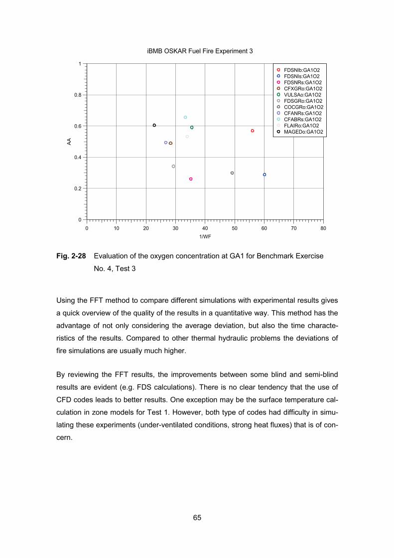
65


0 10 20 30 40 50 60 70 801/WF

0

0.2

0.4

0.6

0.8

1A

AFDSNIb:GA1O2FDSNIs:GA1O2FDSNRs:GA1O2CFXGRo:GA1O2VULSAo:GA1O2FDSGRo:GA1O2COCGRo:GA1O2CFANRs:GA1O2CFABRs:GA1O2FLAIRo:GA1O2MAGEDo:GA1O2

Fig. 2-28 Evaluation of the oxygen concentration at GA1 for Benchmark Exercise

No. 4, Test 3

Using the FFT method to compare different simulations with experimental results gives

a quick overview of the quality of the results in a quantitative way. This method has the

advantage of not only considering the average deviation, but also the time characte-

ristics of the results. Compared to other thermal hydraulic problems the deviations of

fire simulations are usually much higher.

By reviewing the FFT results, the improvements between some blind and semi-blind

results are evident (e.g. FDS calculations). There is no clear tendency that the use of

CFD codes leads to better results. One exception may be the surface temperature cal-

culation in zone models for Test 1. However, both type of codes had difficulty in simu-

lating these experiments (under-ventilated conditions, strong heat fluxes) that is of con-

cern.

66

2.4.4 Discussion

The code to code comparison is already presented in /KLE 06/. Here the main conclu-

sions based on the code to code comparison and the results of the FFT analysis are

discussed.

Additional Uncertainty Based on Blind Calculations

For Benchmark Exercise No. 4 some blind calculations have been performed with FDS

and JASMINE. Regarding the atmospheric temperatures, the AA value is about a factor

of 2 higher for blind calculations compared to semi-blind calculations. The situation is

somewhat better for surface temperatures, although the deviations of the surface tem-

peratures are quite high. It has to be pointed out though that only few results are com-

pared here and these may not be representative. However, the possible influence of

pyrolysis rate is evident.

There have been some discussions on the Benchmark process and the calculational

procedure. With the process used in this project, blind calculations performed with vari-

ous additional input parameters estimated separately by each participant, it is not poss-

ible to identify the reasons for the discrepancies between calculations and experimental

data. Anyway, this shows the effect of unknown boundary conditions as is also the

case for real applications. Additionally, real applications are usually more complex.

Therefore, an additional uncertainty factor (about 2) has to be added to the existing

model uncertainty under known boundary conditions.

Pyrolysis Rate

There is some additional uncertainty on the measured pyrolysis rate. Therefore, the re-

sults have been compared only up to 800 s. Fig. 2-29 shows the comparison of meas-

ured burned fuel mass rates for Tests 1 and 3. In the initial phase, the pyrolysis rate is

slightly higher in Test 3. Later, the trend is reversed due to the lower oxygen concentra-

tion.

67

Pyrolysis rate of OSKAR Fuel Fire Tests 1 & 3

0

10

20

30

40

50

60

70

0 200 400 600 800 1000

Time t [s]

Bur

ned

Fuel

[kg]

Test 1Test 3

Fig. 2-29 Measured burned fuel mass of Benchmark Exercise No. 4, Tests 1 and 3

Atmospheric Gas Temperature and Shift of the Plume

In the following section the temperature predictions at the measurement level 2 are

compared with the experiment. The main focus will be on the temperature distribution

between the front side close to the opening and the backside of the compartment. The

results are compared at about 600 s (see to analyze the shift of the plume the tempera-

ture distribution at level 2 is considered. The temperature difference M12 – M11 be-

tween backside and front side is somewhat larger for Test 1 compared to Test 3. The

JASMINE calculations show a strong temperature difference between M12 and M14 for

both tests. This indicates a strong shift of the fire plume, which was not found in the

experiments. For all other CFD calculations the distribution seems to be more homo-

geneous compared to that of the experiment. However, most of the results concerning

temperature distribution are within in range of uncertainty of the measurement data.

The lumped parameter code COCOSYS does not use the momentum balance. There-

fore, this code is not able to calculate a plume shift. Due to the higher oxygen concen-

tration close to the opening, the front side temperatures are even higher (Tab. 2-13).)

Only semi-blind and open calculations are considered.

68

To analyze the shift of the plume the temperature distribution at level 2 is considered.

The temperature difference M12 – M11 between backside and front side is somewhat

larger for Test 1 compared to Test 3. The JASMINE calculations show a strong tem-

perature difference between M12 and M14 for both tests. This indicates a strong shift

of the fire plume, which was not found in the experiments. For all other CFD calcula-

tions the distribution seems to be more homogeneous compared to that of the experi-

ment. However, most of the results concerning temperature distribution are within in

range of uncertainty of the measurement data. The lumped parameter code COCOSYS

does not use the momentum balance. Therefore, this code is not able to calculate a

plume shift. Due to the higher oxygen concentration close to the opening, the front side

temperatures are even higher.

Tab. 2-13 Temperatures M11 - M14 at about 600 s for Benchmark Exercise No. 4

Test 1

Code M11 M12 ∆M12-11

M13 ∆M13-11

M14 ∆M14-11

Exp 415 592 177 459 44 583 168

FDSNIs 507 618 111 483 -24 631 124

FDSNRs 527 584 57 503 -24 535 8

JASBRs 430 801 371 442 12 426 -4

CFXGRo 510 653 143 567 57 549 39

COCGRo 661 578 -83 630 -31 593 -68

Test 3

Code M11 M12 ∆M12-11

M13 ∆M13-11

M14 ∆M14-11

Exp 560 682 122 571 11 620 60

FDSNIs 461 532 71 464 3 551 90

FDSNRs 432 425 -7 425 -7 486 54

JASBRs 525 782 257 525 0 591 66

CFXGRo 577 564 -13 553 -24 584 7

VULSAo 599 620 21 - - - -

FDSGRo 533 601 68 545 12 525 -8

JASBRo 458 742 284 464 6 475 17

COCGRo 555 489 -66 537 -18 533 -22

69

To analyze the shift of the plume the temperature distribution at level 2 is considered.

The temperature difference M12 – M11 between backside and front side is somewhat

larger for Test 1 compared to Test 3. The JASMINE calculations show a strong tem-

perature difference between M12 and M14 for both tests. This indicates a strong shift

of the fire plume, which was not found in the experiments. For all other CFD calcula-

tions the distribution seems to be more homogeneous compared to that of the experi-

ment. However, most of the results concerning temperature distribution are within in

range of uncertainty of the measurement data. The lumped parameter code COCOSYS

does not use the momentum balance. Therefore, this code is not able to calculate a

plume shift. Due to the higher oxygen concentration close to the opening, the front side

temperatures are even higher.

Tab. 2-13 indicates that both semi-blind FDS calculations at about 600 s indicate lower

temperatures for Test 3 compared to Test 1. This is underlined in Fig. 2-30 indicating

that the continuous temperature increase in Test 3 is not well reproduced. This figure

underscores that it is important not to just analyze peak temperatures only. It is neces-

sary to evaluate the time characteristic of the results too, because possible fire propa-

gation strongly depends on the time characteristic of the thermo dynamics inside the

fire compartment.

70

iBMB OSKAR Fuel Fire Test 1 & 3

0

200

400

600

800

1000

1200

0 500 1000 1500 2000Time t [s]

Tem

pera

ture

M11

[°C

]

Exp-T1-M11FDSNIsT1-M11Exp-T3-M11FDSNIs-T3-M11FDSNRs-T1-M11FDSNRs-T3-M11

iBMB OSKAR Fuel Fire Test 1 & 3

0

200

400

600

800

1000

1200

0 500 1000 1500 2000Time t [s]

Tem

pera

ture

M11

[°C

]

Exp-T1-M11FDSNIsT1-M11Exp-T3-M11FDSNIs-T3-M11FDSNRs-T1-M11FDSNRs-T3-M11

Fig. 2-30 Comparison of atmospheric temperatures between Benchmark Exercise

No. 4, Tests 1 and 3

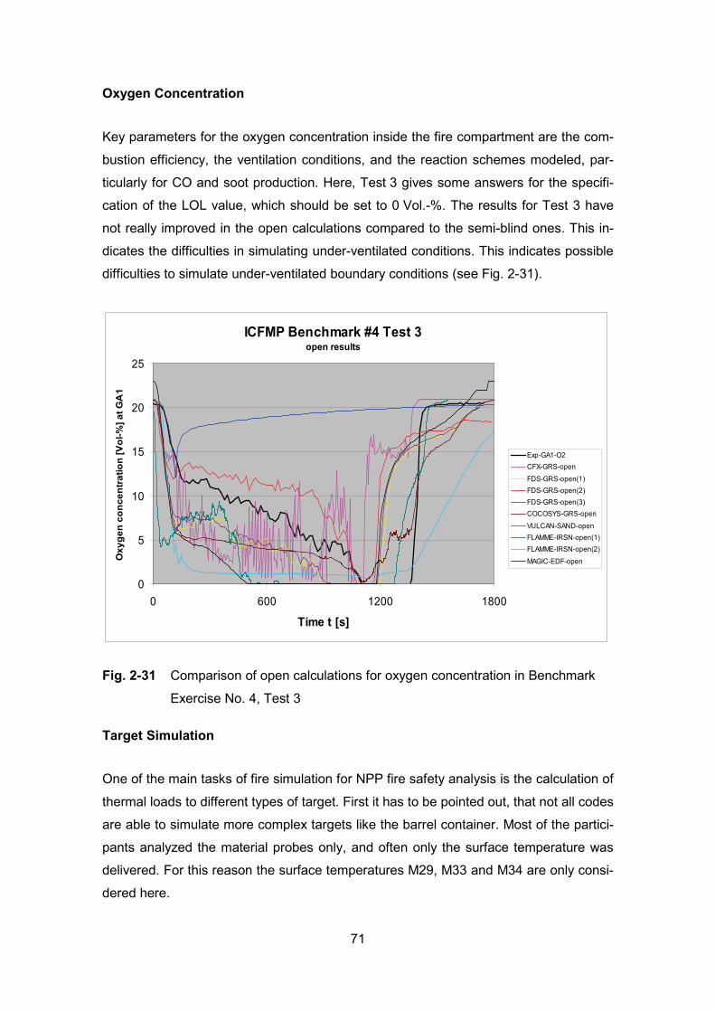
71

Oxygen Concentration

Key parameters for the oxygen concentration inside the fire compartment are the com-

bustion efficiency, the ventilation conditions, and the reaction schemes modeled, par-

ticularly for CO and soot production. Here, Test 3 gives some answers for the specifi-

cation of the LOL value, which should be set to 0 Vol.-%. The results for Test 3 have

not really improved in the open calculations compared to the semi-blind ones. This in-

dicates the difficulties in simulating under-ventilated conditions. This indicates possible

difficulties to simulate under-ventilated boundary conditions (see Fig. 2-31).

ICFMP Benchmark #4 Test 3open results

0

5

10

15

20

25

0 600 1200 1800

Time t [s]

Oxy

gen

conc

entr

atio

n [V

ol-%

] at G

A1

Exp-GA1-O2CFX-GRS-open

FDS-GRS-open(1)FDS-GRS-open(2)FDS-GRS-open(3)COCOSYS-GRS-open

VULCAN-SAND-openFLAMME-IRSN-open(1)FLAMME-IRSN-open(2)

MAGIC-EDF-open

Fig. 2-31 Comparison of open calculations for oxygen concentration in Benchmark


Target Simulation

One of the main tasks of fire simulation for NPP fire safety analysis is the calculation of

thermal loads to different types of target. First it has to be pointed out, that not all codes

are able to simulate more complex targets like the barrel container. Most of the partici-

pants analyzed the material probes only, and often only the surface temperature was

delivered. For this reason the surface temperatures M29, M33 and M34 are only consi-

dered here.

72

Based on the FFT analysis it is seen that the deviations of some code are larger for

Test 1. As an example, the results for the surface temperature at the concrete type

material probe are repeated here to obtain an understanding about the possible devia-

tions (see Fig. 2-32).

ICFM

P B

ench

mar

k #4

Tes

t 1bl

ind

& s

emi-b

lind

resu

lts

0

100

200

300

400

500

600

060

012

0018

00

Tim

e t [

s]

Probe Temperature T [°C ] at M33

Exp-

M33

FDS-

NIS

T-bl

ind

JASM

INE-

BRE-

blin

d(1)

JASM

INE-

BRE-

blin

d(2)

FDS-

NIS

T-se

mi

FDS-

NR

C-s

emi

JASM

INE-

BRE-

sem

iC

FAST

-BR

E-se

mi(1

)C

FAST

-BR

E-se

mi(2

)C

FAST

-BR

E-se

mi(3

)C

FAST

-NR

C-s

emi

ICFM

P B

ench

mar

k #4

Tes

t 1op

en re

sults

0

100

200

300

400

500

600

700

800

060

012

0018

00

Tim

e t [

s]


Exp

-M33

MAG

IC-E

DF-

open

ICFM

P B

ench

mar

k #4

Tes

t 3bl

ind

& s

emi-b

lind

resu

lts

0

100

200

300

400

500

600

700

800

060

012

0018

00

Tim

e t [

s]


Exp-

M33

FDS-

NIS

T-bl

ind

JASM

INE-

BRE-

blin

d(1)

JASM

INE-

BRE-

blin

d(2)

JASM

INE-

BRE-

blin

d(3)

FDS-

NIS

T-se

mi

FDS-

NR

C-s

emi

JASM

INE-

BRE-

sem

iC

FAST

-BR

E-se

mi(1

)C

FAST

-BR

E-se

mi(2

)C

FAST

-BR

E-se

mi(3

)C

FAST

-NR

C-s

emi

ICFM

P B

ench

mar

k #4

Tes

t 3op

en re

sults

0

100

200

300

400

500

600

700

800

060

012

0018

00

Tim

e t [

s]


Exp

-M33

FDS

-GR

S-o

pen(

1)FD

S-G

RS

-ope

n(2)

FDS

-GR

S-o

pen(

3)

VULC

AN-S

AND

-ope

nM

AGIC

-ED

F-op

en

Fig.

2-3

2 C

ompa

rison

of t

he c

oncr

ete

surfa

ce te

mpe

ratu

re M

33 fo

r Ben

chm

ark

Exer

cise

No.

4, T

ests

1 a

nd 3

73

74

2.4.5 Conclusions

The fuel pool fire Tests 1 and 3, performed in the OSKAR test facility at iBMB, Univer-

sity of Braunschweig - Institute of Technology at the end of 2003, have been included

in the benchmarking and validation exercises of the International Collaborative Fire

Model Project as Exercise No. 4. The main difference between the two experiments

carried out is the size of the door area. Both experiments give first indications on the

effects of ventilation and fuel controlled fires as well as on the thermal loading on dif-

ferent types of targets. Previous Benchmark Exercises within the ICFMP had shown

that the simulation of these two phenomena should be improved.

During the Benchmark procedure, the participants performed different types of calcula-

tions. These were totally blind simulations without knowledge of any of the measure-

ments, semi-blind calculations with knowledge of the pyrolysis rate only, and com-

pletely open calculations with knowledge of all experimental results. It has been dem-

onstrated that the pyrolysis rate has a strong influence on the calculation results. Li-

mited information on the pyrolysis rate affects the results to some extent. This finding

was supported from the comparison of the (admittedly few) blind and semi-blind simu-

lations. This overall result of Benchmark Exercise No. 4 should be somehow con-

sidered in the estimation of uncertainty parameters as an input in, for example, PSA

studies.

The simulation of under-ventilated fires is more difficult for the fire codes. In particular,

the high transient behavior at the final phase of Test 3 leads to a wide range of simula-

tion results. Unfortunately, the measured pyrolysis rate is no longer valid in this phase,

and so the ‘specified’ pyrolysis rate may not be reliable at this time. It should be men-

tioned, however, that many of the possible fire scenarios in real nuclear power plants

will lead to under-ventilated conditions. Therefore, this issue should be further investi-

gated and the models should be further improved.

Some codes have difficulty in simulating more complex targets. Most of the codes are

able to simulate the material probes. The range of the results is larger compared to that

for the gas temperatures. As this information is significant for estimating failures of

safety related equipment, the models should be further developed and enhanced.

75


This chapter represents the summary of the ICFMP Benchmark Exercise No. 5: Flame

Spread in Cable Tray Fires. Four full-scale cable tray fire experiments, carried out at

iBMB, University of Braunschweig – Institute of Technology, were used. Detailed infor-

mation about the specification, the experimental results and the results of the calcula-

tions that have been performed are provided in /RIE 06/. Benchmark Exercise No. 5

has considered the results of cable fire experiments with different types of cables, car-

ried out in support of various projects for the German authorities as well as for nuclear

industry in the past /HOS 98/ and /HOS 03/.


A major objective of the actual cable fire experimental series was the investigation of

the effects of a naturally ventilated fire on vertically routed (worst case) bundled power

and I&C (instrumentation & control) cables with different cable insulation materials

(PVC (polyvinyl chloride) and FRNC (fire retardant non-corrosive)). PVC and FRNC

cables are frequently used in German nuclear power plants and also represent stan-

dard cables in other NPP worldwide PVC cable insulation is chemically a thermoplastic

and a typical FRNC cable insulation is a thermosetting material. It has been found

/HOS 03/ that pre-heating of a cable could have strong effects on its fire behavior.

Therefore pre-heating effects have been investigated in Benchmark Exercise No. 5.

Four experiments have been performed, two tests with FRNC cables (Test 1 without

pre-heating and Test 2 with pre-heating) and two tests with PVC cables (Test 3 without

pre-heating and Test 4 with pre-heating).

The measured data from the experiments are the basis for fire simulations by the insti-

tutions from different countries participating in the ICFMP. Four different fire models

have been examined: CFAST, COCOSYS, FDS and CFX. The list of calculations per-

formed is given in Tab. 2-14. A major question for Benchmark Exercise No. 5 was

whether the state of the art computational fire codes are able to predict the pyrolysis

process, and in consequence the flame spread, of burning cable bundles in a given fire

scenario.

76

Tab. 2-14 Models used for Benchmark Exercise No. 5

Model Type

Code Code Version

Modeler (In-stitution)

Blind (b), Open (o)

Calculation

Tests Calcu-lated

Zone CFAST 3.1.7 M. Dey (NRC/NIST)

o1 Test 4

Lumped Parameter

COCOSYS 2.2dev W. Klein-Heßling (GRS)

b o

Test 1, Test 3 Test 1 - Test 4

CFD CFX 10.0 M. Heitsch (GRS)

o Test 1

FDS

4.0 K. McGrattan (NIST)

b, o Test 1 - Test 4

3.1.5 M. Dey (NRC/NIST)

o Test 4 1

1 open calculation: Tests are simulated only for the first 20 minutes (phase of pre-heating)

Another important aspect of cable fires in nuclear power plants is the risk of functional

failures. Therefore within these tests short circuits as well as the loss of conductivity of

the cables have been measured.


The four cable fire experiments have been carried out in a special fire compartment

(iBMB test facility, see Fig. 2-33) with an inner floor area of 3.6 m x 3.6 m = 12.96 m².

The inner compartment height is 5.6 m, giving a compartment volume of 72.6 m³ re-

spectively. Note that the same test facility has been used for Benchmark Exercise

No. 4. The air exchange takes place through an opening of 0.7 m width and 3.6 m

height, which is reduced by a wall of 1.4 m height to an area of approx. 1.5 m². Smoke

gases released are collected in a hood with an exhaust duct located over the opening

and leading to a smoke gas cleaning system. The gases are analyzed according to ISO

9705 /ISO 93/ and the heat release rate has been derived.

In case of pre-heating a pool fire of 0.5 m² pool area, filled with ethanol, has provided

the primary pilot fire. During the phase of pre-heating a maximum gas temperature of

200 °C has been measured close to the surface of the cables. For measuring the mass

loss rate of the liquid pool, the pan has been mounted on a weight scale.

77

The cable tray is directly ignited / inflamed by means of a propane gas burner. In the

case of FRNC cables 150 kW output power and in the case of PVC cables 50 kW out-

put power has been used. In case of pre-heating (Test 2 and Test 4) the ignition burner

is activated after 1200 s. The pre-fabricated 4 m height trays filled with bundled cables

are mounted on a weight scale. Fig. 2-34 shows a diagram of a vertical tray with two

bundles (left side) and (right side) the positions for the temperature measurements on

the surface and in the center of the cables (T, two positions each, at 9 levels), and the

position of the heat flux (WS, 5 levels) and the function loss measurements (FL) at 12

individual cable conductors from cables at the right and left side of the both cable bun-

dles.

Fig. 2-33 Top view of the fire compartment for the Benchmark Exercise No. 5 cable

fire tests (iBMB test facility)

z

y

x

cable tray: 4 m

door / opening: 1.5 m²

pool: 0.5 x 0.5 m²

wall:1.4 m

hood fire compart-

gas burner

78

T FL FL

FL: Function loss test, T: Temperature, WS: Heat flux

TCI 1 TCO 1 TCI 2 TCO 2

TCO 3 TCI 3

WS 1-5 WS

Fig. 2-34 Vertical cable tray: Cross section of two cable bundles on the tray, left:

power cables, right: I&C cables and measurement points

During Benchmark Exercise No. 5 intensive work has been done to provide modelers

with thermo-physical input data for the cables. Different types of tests have been per-

formed, but specially Cone-Calorimeter experiments. The critical heat flux, ignition

temperature, effective heat of combustion, density, thermal conductivity and specific

heat values are given for the sheath insulation material. For the heat of gasification

only an effective value could be derived from Cone-Calorimeter data.

2.5.3 Results

Experiments

A brief overview over the results from the Benchmark Exercise No. 5 test series is giv-

en in the next two figures. The HRR from Test 1 (FRNC, without pre-heating) and Test

2 (FRNC, with pre-heating) and the corresponding ignition burner power output are

shown in Fig. 2-35 and for Test 3 (PVC, without pre-heating) and Test 4 (PVC, with

pre-heating) in Fig. 2-36, accordingly. The pre-heating times from Test 2 and Test 4 of

1200 s are neglected in the figures for comparison. The heat release rate resulting from

the combustible material is low in the case of FRNC insulation material (see Fig. 2-35).

In case of pre-heating, slightly higher values are observed, with a maximum of up to

100 kW. An increase of the burner output of up to 300 kW after 1800 s (Test 2) and

2400 s (Test 1), respectively, have no significant effects on the HRR. In case of PVC

insulation material (see Fig. 2-36, Test 3), the cables (power cables as well as I&C

cables) ignited after a short time and a heat release rate with a peak at 330 kW after

79

approx. 720 s (12 min). In case of Test 4 (see Fig. 2-36) with pre-heated cables, the

I&C cables ignited notably later and the power cables could not be ignited with a 50 kW

burner power output. As a consequence of increasing the burner capacity to up to

100 kW after approx. 900 s (15 min), the power cables ignited and a second peak heat

release rate at 200 kW was found.

The tests show that the FRNC insulated cables have significantly better characteristics

in case of fire. No substantial flame spread takes place in Test 1, even in case of pre-

heating up to 200 °C in the vicinity of the cables in Test 2. While PVC insulated cables

could be ignited with a burner output of 50 kW, for FRNC cables a burner output of

150 kW was necessary.

0 300 600 900 1200 1500 1800 2100 2400

Time [s]

0

50

100

150

200

250

300

350

HR

R, pow

er outp

Test 1, FRNC (without PH) cable bundles gas burner

Test 2, FRNC (with PH) cable bundles gas burner

Fig. 2-35 Heat release rate (HRR) of FRNC cable bundles and gas burner power

output for Benchmark Exercise No. 5, Tests 1 and 2, with and without pre-

heating (PH)

In Test 3, a continuous average flame spread rate from 40 cm/min over the length of

the cable tray has been derived from the experimental data for I&C cables. In Test 4

(PVC, with pre-heating) the power cables could not ignited with 50 kW power output

from the gas burner, but could with 100 kW. It has been concluded that it is difficult to

interpret the influence of pre-heating on ignition and flame spread.

80

The test series indicate that the burning behavior of a pre-heated PVC cable is similar

to that of an aged PVC cable. If a flammable cable is pre-heated then plasticizers could

emit from the cable, a process which normally leads to better fire characteristics.

0 300 600 900 1200 1500 1800 2100 2400

Time [s]

0

50

100

150

200

250

300

350

HR

R, pow

er outp

Test 3, PVC (without PH) cable bundles gas burner

Test 4, PVC (with PH) cable bundles gas burner

Fig. 2-36 Heat release rate (HRR) of PVC cable bundles and gas burner power out-

put for Benchmark Exercise No. 5, Tests 3 and 4, with and without

pre-heating (PH)

Function Loss Tests

Short circuits occur first as ‘conductor to conductor’ shorts and later as ‘conductor to

tray’ shorts (shorts to ground). The time period until short circuits occur strongly de-

pends on the pre-heating of the cables. Without pre-heating, the short circuit times are

a factor of two higher than in case of pre-heating. In one case with pre-heating PVC in-

sulated I&C cables failed after only 100 s. The average time to loss of function of PVC

insulated I&C cables with pre-heating, according to the experiments, is approx. 220 s.

The short circuit times of power cables are nearly two times higher than those of I&C

cables and are independent of the cable insulation material. FRNC insulated cables

show better characteristics in all tests and are ignited with a substantially higher burner

output as mentioned above. For further details see /RIE 06/

81

Calculations

In Tab. 2-15 details about the different fire models used in Benchmark Exercise No. 5

are given. Blind and open calculations have been performed. On the basis of the re-

sults from the blind calculations the COCOSYS code has been enhanced in two re-

spects:

− The heat transfer into the cables close to the burner has been improved,

− A remaining mass fraction for incomplete burn down of cables has been intro-

duced.

In the other fire models no changes in the code have been made in the versions that

have been used.

Additional calculations have been performed by M. Dey (NRC/NIST) with FDS (CFD)

and CFAST (zone model). These calculations are restricted to Test 4 (PVC insulated

cables) and only the time of pre-heating (first 1200 s) has been considered. The calcu-

lations have been used to study the performance of the two codes considering a sce-

nario of an ethanol pool fire. Because this work was not conducted with the intention to

study flame spread phenomena it will not be discussed in this summary. Nevertheless,

this work does give information about the performance of two models if the heat re-

lease rate is given.

In Fig. 2-37 the measured pyrolysis rate of the cables (MLR_Cables), the input (CFX,

COCOSYS) and the calculated MLR_Cables (FDS) for Test 1 (FRNC, no pre-heating)

is shown as an example for the ‘results’ of the open calculations. In this context, note

that only FDS has a sub-model to predict the pyrolysis rate of a burning object. Fig.

2-38 shows the measured and the calculated surface temperature of the I&C cables at

the cable tray at 1.5 m height (2 m above the compartment ground) again for Test 1.

82

Tab. 2-15 Details on the different fire models used in Benchmark Exercise No. 5

regarding the pyrolysis rate for modeling flame spread on a cable tray

Model Type Lumped Parameter CFD

Code Code Type

COCOSYS 2.2 developer ver-

sion

FDS 4.0 CFX 10.0


W. Klein-Heßling (GRS)

K. McGrattan (NIST)

M. Heitsch (GRS)

Cable bundle one rectangular slab

without core one rectangular slab

without core one rectangular slab

with metal core

Thermal model cable slab

1-dimensional (only side of burner)

1-dimensional (all sides indepen-

dent)

3-dimensional

Pyrolysis model

empirical data finite rate experimental data

Calculation of pyrolysis rate

pyrolysis rates for different material temperatures de-

rived from database

pyrolysis rate in the environment of a giv-en ignition tempera-

ture is calculated with an Arrhenius law

(thermoplastic model)

a fixed pyrolysis rate is used, when a given

ignition temperature is reached at one point at

the cable slab

Data (input) pyrolysis rates at different material temperatures are

derived from differ-ent (older) tests in the same facility

thermal properties, heat of gasification

and ignition tempera-ture from given Cone

Calorimeter data

pyrolysis rate from test results of Benchmark

Exercise No. 5

Possibility of prediction

in principle yes No

83

Model Type Lumped Parameter CFD

Code Code Type

COCOSYS 2.2 developer ver-

sion

FDS 4.0 CFX 10.0


W. Klein-Heßling (GRS)

K. McGrattan (NIST)

M. Heitsch (GRS)

Performance of prediction of pyrolysis rate for PVC and FRNC cables

PVC: pyrolysis rate is ‘calculated’ in ac-ceptable agreement; FRNC: pyrolysis rate

is ‘calculated’ ex-tremely high (for

open calculations it is set to zero)

PVC: pyrolysis rate too low;

FRNC: pyrolysis rate too high

(pyrolysis rate is given as input)

Performance of prediction of surface temperature

PVC: results are acceptable for such kind of calculation; FRNC: great differ-

ences

behavior of a ther-moplastic material, if pyrolysis takes place;

the material burns nearly at a given igni-

tion temperature

FRNC: temperatures in the near field of the

ignition burner compa-rable, in the far field too

low

Remark: universality of the database is not

proven

the only model with a ‘real’ pyrolysis model

included

only Test 1 has been simulated

0 1000 2000 3000 4000 5000

Time [s]

-0,001

0,000

0,001

0,002

0,003

0,004

0,005

0,006

Pyrolysis rate cab

Test 1, MLR_Cables Exp. COCOSYS FDS CFX

Fig. 2-37 FRNC cables pyrolysis rates (MLR_Cables) for Benchmark Exercise No. 5,

Test 1 – comparison of experimental data, input data and code calculations

predicted

measured

set to zero

from experiment

84

0 1000 2000 3000 4000 5000

Time [s]

0

100

200

300

400

500

600

700

Cable surface tem

Test 1, TCO3_3 Exp. COCOSYS FDS CFX

Fig. 2-38 FRNC I&C cable surface temperatures (TCO3_3) for Benchmark Exercise

No. 5, Test 1 - comparison of measured data and calculation results

In FDS a thermoplastic pyrolysis model has been deployed and the specified thermo-

physical data derived from experimental Cone Calorimeter measurements have been

used as input. In the model, nothing accounts for charring or for the lateral heat con-

duction in the metal core. Furthermore, the complex cable bundle structure must be

replaced with a rectangular slab because of the structure of the underlying numerical

grid. The thickness of the solid is not fixed to the gas phase grid, only the exposed sur-

face area. The calculated gas temperatures in the direct environment of the cable tray

are in a good agreement with the experimental data. But the calculated heat fluxes did

not follow the experimental results and are notably too low (see Fig. 2-39, Test 2, upper

one). The predicted pyrolysis rates are slightly too high in the case of FRNC cables

(Test 1 and Test 2) and too low in case of PVC cables (Test 3 and Test 4). If pyrolysis

takes place the material starts burning nearly at a given ignition temperature. This is

the effect of the use of a thermoplastic model. In this case the predicted cable surface

temperatures did not follow the experimatal data (see Fig. 2-39, Test 3, lower one).

85

Test 2, Heat Flux to Cable Tray

Time (min)

0 5 10 15 20 25 30

Hea

t Flu

x (k

W/m

2 )

0

1

2

3

4

5

6

Exp Time vs WS1 Exp Time vs WS3 Exp Time vs WS5 FDS Time vs WS 1 FDS Time vs WS 3 FDS Time vs WS 5

Test 3, I&C Cable Surface Temperatures

Time (min)

0 5 10 15 20

Tem

pera

ture

(C)

0

100

200

300

400

Exp Time vs TCO 3-1 Exp Time vs TCO 3-3 Exp Time vs TCO 3-5 FDS Time vs TCO 3--1 FDS Time vs TCO 3--3 FDS Time vs TCO 3--5

Fig. 2-39 FDS predictions for Benchmark Exercise No. 5 - Heat flux to cable tray

(Test 2, left side), PVC I&C cable surface temperatures (Test 3, right side)

In COCOSYS, an empirical approach has been chosen to calculate the heat release

rate and the flame spread of a given cable tray fire scenario. The model uses a speci-

fied pyrolysis rate for the cables, represented also by a rectangular slab. The propaga-

tion velocity depends on the assigned surrounding temperature of the target. A data-

base for this property was derived from earlier experimental results, obtained in the

same compartment under similar conditions. During the ICFMP Benchmark calcula-

tions, the COCOSYS code was further developed in various respects. The heat trans-

fer into the cables works considerably better now.

86

The calculated cable surface temperatues are in a good agreement with the experi-

mental data (see Fig. 2-40) in the open calculations (blue curves). Some problems still

exist concerning the stability in those zones close to the vertical trays. This problem

has to be solved in the future.

Fig. 2-40 COCOSYS (2.2dev) predictions for Benchmark Exercise No. 5, Test 3 -

PVC power cable surface temperatures

In CFX, while no pyrolysis model is included, the basic elements for checking the igni-

tion temperature at each boundary cell of a solid does exist, and this can be coupled to

a specified pyrolysis rate. The work to build up such a model has been started but is

not yet finished. Because of some problems with this approach only Test 1 of Bench-

mark Exercise No. 5 has been calculated. The exercise to model a burning cable has

therefore been simplified in that a constant pyrolysis rate (from the experimental data)

is initiated once the ignition temperature at any one of the CFD cells at the cable bun-

dle is reached. The calculated gas temperatures are in better agreement with the expe-

rimental data in the direct environment of the cables for the first level of the gas burner

with 150 kW power output. However, the predicted gas temperatures are too low for

the second phase with 300 kW power output (see Fig. 2-41).

87

In consequence, the resulting surface temperatures of the cables do not follow the ex-

perimental data in this phase of the burner output. The original task of Benchmark Ex-

ercise No. 5 was to predict the pyrolysis and not to prescribe it. For the future it will be

of great interest if sub-tools for modeling the pyrolysis of a complex cable can work in a

more sufficient way.

0 2000 4000 6000Time [s]

0

50

100

150

200

250

Tem

pera

ture

[Deg

C]

TR1-2TR1-2, CFXTR1-4TR1-4, CFXTR1-7TR1-7, CFX

TR1-2,4,7

BM5 Test 1

Fig. 2-41 CFX 10.0 predictions for Benchmark Exercise No. 5, Test 1 - Calculated

gas temperatures in the room

2.5.4 Discussion

It should be noted that most of the codes could predict the main quantities such as gas

temperature, heat flux, gas velocity, etc. reasonably well provided the heat release rate

from the fire is given and the fire scenario is not too complex. This has been demon-

strated in the other ICFMP Benchmark Exercises /DEY 02/, /KLE 06/, and /MCG 07/.

However, to predict the HRR and flame spread for a given application, such as in

Benchmark Exercise No. 5, is a completely different task.

It is very difficult to predict HRR and flame spread on complex fire sources such as

cables. As a first step, it would be useful to model a complex object as a collection of

smaller ones, each having properties similar to the solid material.

88

Cable bundles could be treated as a collection of small cylinders, for which the interac-

tion with each other would be almost completely separate from the gas phase grid. As

there are no standards to derive thermo-physical data from a set of Cone Calorimeter

tests, it will be necessary to have clear guidelines for the procedure for determining

such data.

2.5.5 Conclusions

At the time being, none of the codes applied in Benchmark Exercise No. 5 for calculat-

ing the ignition, pyrolysis and flame spread of realistically routed cables work at a level

such that it is possible to use them as a reliable predictive tool for predicting such phe-

nomena. It is obvious that there is a need for the development and enhancement of

sub-models for pyrolysis.

Because of continued flame spread, the data of Test 3 (PVC, no pre-heating) are par-

ticularly appropriate for the validation of fire spread models. The pyrolysis models have

to demonstrate that they can predict the results of Test 1 as well as those of Test 2,

because no flame spread occurs in the case of FRNC cables. This may indicate that a

computer code, which just performs well if flame spread occurs, may not be suitable to

handle complex materials.

For a development of pyrolysis models for cables more small-scale cable fire experi-

ments have to be performed and only one parameter should change per test. Pre-

heating effects, different insulation materials, orientation, all play an important role in a

realistic cable fire.

Benchmark Exercise No. 5 also shows that the input parameters for a pyrolysis model

are highly sensitive, since a model will work only with the correct thermo-physical data

for the material used. Up to now, there are no set rules on how to measure the different

properties, such as heat of gasification, ignition temperature and heat of combustion.

Because of the complexity in developing a complete deterministic flame spread model

for cables there is a need for further measurement of empirical data for fire spread (py-

rolysis growth) on complex items, e.g. cable trays.

89

3 Discussion

3.1 Project Accomplishment and Participants Perspectives

Since commencing in October 1999, the project has made significant progress towards

achieving its original goals. For Phase I the primary objective was to examine the ca-

pability of current numerical fire models by means of a series of Benchmark Exercises

conducted by participating organizations, and this has now been completed with some

success. A broad selection of representative fire models has been examined, ranging

from hand-calculations and spreadsheet applications, through zone and lumped-

parameter models to the most computationally demanding, namely CFD. While partici-

pants were from Europe and the United States only, they came from diverse back-

grounds, ranging from fire engineering students, consulting firms, public bodies to the

code developers themselves.

A wide range of scenarios have been examined in the five Benchmark Exercises, rang-

ing from relatively small rooms to a turbine hall size enclosure, and from simple box-

like geometries to more complex examples with multiple compartments or sloping

roofs. Local as well as fully-developed (post-flashover) fires have been included, and in

some cases the fires have been ventilation controlled. Natural and mechanical ventila-

tion has been studied.

A combination of blind, semi-blind and open calculations have been conducted to help

verify and validate the selected fire models and fire modeling approaches for the range

of scenarios investigated. This has contributed to the verification and validation process

for the different fire modeling approaches (zone, CFD, etc.). Conclusions have been

drawn regarding where fire models can reliably be used, and also where more caution

is required. In depth analysis of the results from the Benchmark Exercises has allowed

the strengths and weaknesses of the current generation of fire models to be reviewed,

and to identify where further advances are required. The work has laid the foundation

for the generation of guidance on the use and interpretation of fire models for nuclear

power plant applications.

The results of the ICFMP have identified a range of phenomena which all types of fire

models can be expected to predict with some reasonable degree of accuracy.

90

All models predicted, with some confidence, hot gas layer temperature and depth, once

the fire power and boundary heat losses were properly accounted for, and where the

fire was well ventilated and the geometry not overly complex, e.g. in the near-sealed

upper deck turbine hall case in Benchmark Exercise No. 2. Oxygen depletion, i.e. the

onset of conditions where combustion is likely to cease due to a lack of oxygen, was

similarly reasonably well predicted by the range of fire models investigated. Vent flow

through vertical openings, e.g. doors, was as expected a straightforward task in most

cases.

It has been demonstrated that zone models are able to account for irregular ceiling

shapes provided the volume of the space is included appropriately and the layer depth

interpreted correctly, e.g. in Benchmark Exercise No. 2. Although requiring some effort,

mechanical ventilation was applied successfully in the application of zone models.

Cases where local three-dimensional effects are important, e.g. the maximum tem-

perature under a ceiling where a fire plume impinges, could be predicted by CFD and,

perhaps to a lesser extent, lumped-parameter models. Furthermore, while difficult for

general two-layer zone models, post-flashover fire conditions could be reasonably

modeled by CFD and lumped-parameter models, e.g. in Benchmark Exercise No. 4.

As important as clarifying where models can be reliably applied, is to identify where

they are not currently suited, and the ICFMP has made important contributions here. Of

particular relevance to nuclear power plants is the challenging task of predicting the

response of cables and cable bundles subject to fire conditions, and ultimately to pre-

dict spread of fire along a cable or within a cable tray. Benchmark Exercise No. 5 dem-

onstrated that this remains a challenge for existing cable and pyrolysis sub-models and

that these models need improvement to provide more accurate predictions of cable

fires. Nonetheless, an empirical based approach, using experimentally measured cable

behavior information as an integral part of the fire model, may offer a short term solu-

tion. It should be noted that it is not only the thermal response and electrical failure of

the cable that is difficult to predict, but also the modeling of the incident flux to the ca-

ble. The challenge of predicting thermal fluxes, and in particular radiation fluxes where

the T4 dependence makes the phenomena highly nonlinear, was shown to be a main

area of uncertainly in fire modeling in all Benchmark Exercises.

91

While predicting the pyrolysis (burning rate) of cables is understandably a very difficult

task calculating the pyrolysis of ‘simpler’ fuels such as hydrocarbon pools also proved a

challenge. Fire models do not, in general, include a pyrolysis sub-model, and even

where one is provided it is generally in a simple form and unlikely to be very accurate,

as illustrated in Benchmark Exercise No. 4. The fundamental issues are the same as

for cables, i.e. the heat transfer inside the fuel and the incident heat flux are both criti-

cal phenomena that are difficult to model with sufficient accuracy for pyrolysis and fire

spread calculations.

Limitations peculiar to zone models were identified, e.g. predicting flows across hori-

zontal vents as in the turbine hall example in Benchmark Exercise No. 2. Post-

flashover fire conditions also posed a problem for the two-zone fire models investi-

gated.

Some of the problems that can be encountered in verifying and validating fire models

have been identified too. The process adopted in the Benchmark Exercises lent itself

towards a qualitative verification and validation of the fire models. By contrast, the

U.S. NRC Verification and Validation activity /NRC 07/ has adopted a more formal

process, whereby all parameters and sub-model selection choices for the computer

models were tightly specified, and the verification and validation was arguably more

quantitative. However, the U.S. NRC exercise did not include blind calculations, which

is an important contribution made by the ICFMP. Important lessons have been learned

for future benchmarking and analysis.

The ICFMP has allowed modeling tasks and phenomena requiring further development

to be identified. Perhaps most important here is the task of predicting the heating and

failure of safety critical items such as cables. Ignition, pyrolysis and flame spread are

also an important task for which model development is required. In both cases, the use

of empirical measured data may provide a practical near term solution. Other modeling

issues for which further research and development is required include natural flows

through horizontal (e.g. ceiling) vents, in particular for zone models, the prediction of

soot yields and radiation fluxes, and smoke flows between compartments via vents and

ducts.

92

3.2 ICFMP Results from the Benchmark Exercises No. 1 to 5

The results from the five ICFMP Benchmark Exercises have provided important in-

sights into the performance of the current generation of fire models for a wide range of

nuclear power plant applications. The process of blind and open calculation has helped

to identify the strengths and weaknesses of fire models in a robust and trustworthy

way. Comparisons of calculation against experimental measurement, and also of cal-

culation against calculation, have provided an important contribution to this process.

Section 2 of this Summary Report highlights the main results and findings for each

Benchmark Exercise. Below the main uncertainties and parameter sensitivities are dis-

cussed.

3.2.1 Uncertainties

During the course of the ICFMP a number of phenomena and modeling parameters

have been shown either to be inherently uncertain in nature or to lead to uncertainty in

the predictions.

Throughout the ICFMP work the definition of the fire source arguably presented the

biggest uncertainty. Not only are the fire dimensions and pyrolysis rate difficult to spe-

cify, but the physical processes of combustion efficiency, soot and toxic gas yields and

radiative fraction also present challenges to the fire modeler. While it is in theory possi-

ble to model these phenomena, in practice they generally require ‘engineering judg-

ment’.

For blind calculations the choice of the pyrolysis rate will obviously lead to uncertainties

if the actual rate, subsequently used in open calculations, deviates to any significant

extent from the value in the actual experiment. For a well controlled fire, e.g. as in

Benchmark Exercise No. 3, this should ideally be only a second order uncertainty. For

fire sources with less control, e.g. fuel pool, wood crib or other more complicated ob-

jects, the uncertainly introduced may be quite significant, as illustrated in Bench-

mark Exercise No. 4. However, even for the ‘simpler’ fire sources such as a spay burn-

er there may be a notable deviation between prior estimation and actual value. For

Benchmark Exercise No. 3 the actual pyrolysis (fuel supply) rate varied by as much as

15 %, which will have influenced the gas temperatures by as much as 10 %.

93

Other quantities may then be subject to even higher uncertainty, e.g. for radiation flux

where the T4

3.2.2 Parameter Sensitivities

dependency is important. Errors in the processing of the experimental

data to derive the fuel supply rate for the semi-blind and open calculations for Bench-

mark Exercise No. 3 illustrated further the significance of experimental uncertainties.

Soot yield and associated radiative fraction, as well as combustion efficiency, are also

significant sources of uncertainty in both blind and open calculations. The soot yield

and radiative source term are particularly important for calculating target response, and

so there is a corresponding significant level of uncertainty in the target heating and

response calculations.

There may be uncertainty in model predictions where the level and details of natural

and/or mechanical ventilation is not well known. In Benchmark Exercise No. 4 a venti-

lation flow through the mechanical ventilation system was known to the analysts but

could only be estimated, and will have had some bearing on the conditions inside the

test enclosure, and perhaps also at the main vent to the outside, i.e. influencing the

distribution of ventilation between the main (door) vent and the mechanical system.

Where enclosures are nearly sealed there is always uncertainly in the actual leakage

(infiltration) area and details. However, the predictions from various Benchmark calcu-

lations involving near sealed compartments were relatively insensitive to the precise

area and location of the modeled leakage. Obviously, below a certain leakage area

pressure effects become important, but otherwise the dependency was not significant.

The physical phenomena and model parameters for which predicted results were most

sensitive are summarized in the following. Re-iterating the point made above, fuel pyro-

lysis rate, whether a user-defined input or calculated by the fire model, is the most sen-

sitive physical parameter. It can significantly influence the predictions, as illustrated in

Benchmark Exercises No. 3 and No. 4, the latter in particular illustrating that the dif-

ference between using estimated (blind) and measured (semi-blind / open) pyrolysis

rates can lead to differences in target temperatures of the order of a factor of two.

Analogous to pyrolysis rate, heat of combustion, combustion efficiency and radiative

fraction are also sensitive parameters.

94

The combination of these three terms controls, to a large extent, the convective power

of the fire, and this in turn directly influences the smoke temperature and entrainment

rate. The appropriate setting of the convective power is important in obtaining a good

match between prediction and measurement for smoke filling cases, as illustrated in

Part I of Benchmark Exercise No. 2 where differences of the order of 15 % were ob-

served in the upper layer temperature for CFAST when varying the convective power

by 40 %.

Soot and combustion product concentrations, in combination with gas temperature,

have a strong influence on radiation fluxes, for which target heating is particularly sen-

sitive. Factors of the order times two in the incident radiation flux to a target were seen

in various Benchmark calculations as a consequence of changes in the gas tempera-

ture field.

Boundary thermal inertia is another sensitive parameter. In the extreme limit, varying

the thermal property of the ceiling and walls of an enclosure from adiabatic (no heat

loss) to highly conducting (e.g. steel) can have an influence greater than those para-

meters directly influencing the convective power of the fire source.

While the above physical parameters are all important in respect to the sensitivity of the

model predictions, perhaps an even more important parameter is the user itself. It is

the user (e.g. fire engineer, computer modeler) who will often decide the radiative frac-

tion, fuel heat of combustion etc., and thus having a significant bearing on the final out-

come of the modeling.

As also indicated above, a number of physical phenomena were found, in the course of

the ICFMP Benchmark Exercises, to only weakly influence the predictions. These in-

clude the choice of ambient values, the setting of lower oxygen limit and the exact de-

tails of enclosure leakage modeling.

95

4 Conclusions

The International Collaborative Fire Modeling Project (ICFMP) has provided an open

international collaborative forum for experts to discuss performance of fire models over

the course of its eight year lifetime from 2000 to 2007. Its accomplishments include:

• Establishing a web portal that allowed members to share information via a discus-

sion forum and a document library,

• Organizing and documenting five Benchmark Exercises that are summarized in this

document,

• Supporting contributions such as a zone model validation database and

• Inspiring new experiments and independent code validation projects.

The ICFMP filled a void at a crucial time from the perspective of the nuclear industry

and its regulatory environment, while the U.S. standard NFPA 805 /NFP 01/ for risk-

informed fire protection was finalized and adopted. Thereafter risk-informed methods

were accepted by the U.S. NRC, and the use of fire modeling was more formally codi-

fied in a joint industry and regulatory guidance document for Fire PSA, NUREG/CR-

6850 /EPR 05/. A new international market for fire modeling services was essentially

developed which required, at its foundation, a solid technical basis for the applicability

of fire models. The ICFMP anticipated this need and its contribution to the required

technical basis is summarized in this document.

The timely need for an organization such as the ICFMP was a major factor in its suc-

cess and the development of the five Benchmark Exercises. Many contributors to the

ICFMP were from government bodies or laboratories, but the open nature of the

ICFMP contributed to its success by allowing contributors from private organizations. It

is important to maximize the number of potential contributors for varied reasons: To

examine user effects on code performance, to increase the talent pool of fire modelers,

and to encourage innovation. The web portal was another contributor to success of the

ICFMP by facilitation correspondence and report preparation between meetings.

The ICFMP could not have existed without financial support of government bodies and

institutions, their willingness to conduct experiments and share data, and their coopera-

tion by providing contributors and resources for ICFMP functions.

96

Experiments were conducted in part due to the influence of the ICFMP. In this regard,

the ICFMP provided an essential international forum that affirmed the need for such

work, and also a forum for use of the experimental data.

New code validation efforts and experiments outside of the ICFMP can be traced to the

existence of the ICFMP. In this regard, the ICFMP provides a foundation for code com-

parison standards, because it inspires a formal code validation report in support of the

U.S. regulation. Also in this regard, the ICFMP provides leadership for the future of fire

science, exemplified by the international collaboration for the PRISME experiments

currently under way in France.

From the technical point of view, the ICFMP Benchmark Exercises have provided im-

portant information:

• From the first Benchmark Exercise, it was clear that while computer codes were

reasonably capable of evaluating a common scenario, user effects were evident

and crucial sub-models and phenomena were noted. This has translated into sensi-

tivity analysis as a good practice in fire modeling for Fire PSA. The accuracy of

blind calculations is particularly impacted by user effects. Differences between

model predictions and experimental results for blind calculations compared to

semi-blind / open calculations demonstrate the difficulty model users face choosing

input values for design model simulations. Guidance documents for nuclear power

plant fire modeling applications are needed to assist model users in choosing ap-

propriate modeling parameters.

• Zone models were shown to be reasonable for evaluation of smoke layer tempera-

ture and elevation, despite complexities associated with some experimental confi-

gurations. Variation between results and data could occur for both zone and CFD

models, such as seen with vent flows. Overall, this implies that Fire PSA can be

conducted using zone models, provided that their limitations are recognized,

• User effects continue to be an issue, and user guidance documents that discuss

sensitivity of results to key inputs: Fire heat release rate, vent characteristics, target

detail, etc. would be useful for a nuclear power plant Fire PSA,

• Under-ventilated fire conditions still poses a modeling challenge and

• Modeling of cable pyrolysis, ignition, and flame spreading also poses a substantial

modeling challenge.

97

The ICFMP has supported further the progress of fire modeling and the validation and

verification of computer programs for Fire PSA. The challenges mentioned above

should be taken up by future international collaborative efforts. In addition to the tech-

nical insights described above, this project has provided valuable insights in terms of

techniques for model evaluation. For instance, from this project it is obvious that blind

calculations can provide insights into the user's capabilities and the importance of

model user guidance, but provide less insights into the predictive capability of the mod-

els themselves. Other lessons learned from this project should lead to improvements in

the standard guides for assessing predictive capabilities of fire models.

99

5 Future of the ICFMP

The future of the ICFMP is under discussion during preparation of this Summary Re-

port on Benchmark Exercises No. 1 to 5. Main points of the discussion held during the

April 2007 meeting are presented here. There was no firm consensus on the topic, and

a future workshop was recommended, perhaps in conjunction with a PRISME project

meeting.

The future of the ICFMP essentially is contingent upon several factors:

• Uniqueness of its mission, and the ability to perform work outside the scope of ex-

isting research programs and

• Resources provided by supporting organizations, including the availability of key

personnel who may be involved in related projects,

• Continuation of the open nature of the forum and its ability to obtain non-

proprietary data.

Continuation of the ICFMP is motivated a number of potential projects that transcend

existing national and international programs related to nuclear power plant fire safety. A

list of 10 such projects created by the ICFMP includes suggested Benchmarks and

topical evaluations, and further suggestions were discussed during the April 2007

meeting.

Suggested Benchmark Exercises include:

• Target heating in divided compartments, a topic that is in part investigated by

OECD PRISME project,

• Validation exercises to examine and help resolve issues identified in previous

Benchmarks, notably Benchmark Exercise No. 3 and the suggested divided com-

partment benchmark. New exercises would also focus better on sensitivity analysis

and quantification of uncertainty and

• New fire modeling application exercises for several specifically suggested plant

geometries. Standard problems for model application would use real plant informa-

tion, and the broad issue of fire model applications would be investigated by com-

paring and contrasting the results of various models and modelers.

100

Topical evaluations include:

• Detector response modeling, including evaluation of existing detector codes and

how such models might be applied for nuclear plant applictations,

• A Practical Users Guide providing suggestions on how to model important scenario

features such as heat loss, ventilation, smoke spreading between compartments,

and local effects such as flame impingement,

• Review and suggestion of specific code input data related to generic phenomena,

such as values for flow coefficients,

• Development of heat release rate curves for cable trays,

• Review of cable modeling methods and recommendations for cable dysfunction

criteria and

• Updating the Validation Database Report (VDR) which describes experimental data

pertinent to model application to nuclear power plants.

The uniqueness and openness of ICFMP were identified as significant factors in favor

of its continuation. The list of potential projects above has only minor overlap with cur-

rently existing major programs. These potential ICFMP efforts would be complementary

to those of other programs. Furthermore, such ICFMP efforts are quite timely due to

the increased importance of Fire PSA. The openness of ICFMP is a clear distinguishing

factor that sets ICFMP apart from nearly all existing major programs, since those pro-

grams involve proprietary information within single countries or within chartered organi-

zations of countries. Openness of the ICFMP is an advantage at a time when many

persons are interested in fire modeling for nuclear power plant PSAs.

The resource issue was identified as a significant factor against future ICFMP activity.

This issue has two aspects: Some ICFMP personnel are deeply involved in current

international projects and would probably not have enough time to participate, and the

ICFMP is competing for funding of existing major national and international projects.

The future of the ICFMP will hopefully be resolved at least in 2008 through considera-

tion of the issues presented here.

101

6 Acknowledgements

In addition to the authors identified providing input to this Summary Report, several

experts from various institutions contributed to the ICFMP in many ways.

A group of specialists from different expert institutions participating in the ICFMP con-

tributed to Benchmark Exercise No. 1 as mentioned in /DEY 02/ either through the per-

formance of analysis in the Benchmark Exercise, and/or by providing peer comments

at various stages of the Exercise. The Industry Management Committee, UK and the

National Institute of Standards and Technology (NIST), USA sponsored or collaborated

with the organizations represented at the corresponding meetings.

The experimental measurements for Benchmark Exercise No. 2, Part I were collected

by VTT as part of the European Coal and Steel Community project NFSC2, and are

used by permission of the executive committee, SERDEC.

The test series used for Benchmark Exercise No. 3 was co-sponsored by the US Nu-

clear Regulatory Commission and the National Institute of Standards and Technology

(NIST). Anthony Hamins and Alex Maranghides of NIST conducted the tests. Jonathan

Barnett at Worcester Polytechnic Institute, USA, and Chantal Casselman at IRSN,

France provided project management and technical support to the ICFMP group.

Alan Coutts at WSMS, USA, Jason Floyd at Hughes Associates, USA, Bijan Najafi and

Francisco Joglar-Billoch at SAIC/EPRI, USA, Bernard Gautier and Laurent Gay at EdF,

France, Peter Rew at WS Atkins Consultants, UK, Olaf Riese at iBMB, Germany, Jür-

gen Will at HHP Braunschweig, Germany, Walter Jones at NIST, USA, Robert Kassa-

wara at EPRI, USA, Naeem Iqbal at NRC/NRR, USA, and Alan Wylie and Geoff Jones

at HSE/NII, UK all contributed to Benchmark Exercise No. 3 either by providing peer

comments, participating in meetings to discuss the test plan and results, or indirectly by

sponsoring participants for the project.

The test series used for the Benchmark Exercises No. 4 and 5 were co-sponsored by

Federal Ministry for Economy and Labour (BMWA) within the frame of the project

RS 1146, the German Federal Ministry for the Environment, Nature Conservation and

Nuclear Safety (BMU) and the German Federal Authority for Radiation Protection (BfS)

within the frame of the projects SR 2449 and SR 2491.

102

The tests were performed by Institut für Baustoffe, Massivbau und Brandschutz (iBMB),

University of Braunschweig - Institute of Technology, Germany sub-contracted by GRS.

Dietmar Hosser, Reinhold Dobbernack, Olaf Riese, Hans-Joachim Wolff and Mark

Klingenberg were the key iBMB staff for the Benchmark Exercises No. 4 and No. 5 test

series.

Heinz Peter Berg from BfS, Germany, Chantal Casselman from IRSN (France), Mon-

ideep Dey (USA), Walter-Klein-Heßling from GRS, Germany, and other members of

the institutions participating in the ICFMP project all contributed to the Benchmark Ex-

ercises either by providing peer comments, participating in meetings to discuss the test

plan and results, or indirectly by sponsoring participants for the project.

Olavi Keski-Rahkonen (retired) and Simo Hostikka at VTT, Finland, as well as James

Oldham and Doug Brandes (retired) at Duke Energy, USA hosted the 7th, 8th and 9th

ICFMP meetings where the Benchmark Exercises No. 3 to 5 were planned and dis-

cussed, and also provided peer reviews and technical support.

All the ICFMP Benchmark Exercises as well as this document would not have been

possible without the help and expertise of all the above.

103

7 References

/AST 05/ American Society for Testing and Materials ASTM International

ASTM E1355-05a, Standard Guide for Evaluating the Predictive Capability

of Deterministic Fire Models, ASTM International, West Conshohocken, PA,

www.astm.org, 2005

/DEY 02/ Dey, M. K., Ed.

Evaluation of Fire Models for Nuclear Power Plant Applications: Inter-

national Panel Report on Benchmark Exercise No. 1, Cable Tray Fires,

U.S. Nuclear Regulatory Commission, Office of Nuclear Regulatory Re-

search, NUREG 1758, Washington, June 2002, also National Institute of

Standards and Technology (NIST), NISTIR 6872, June 2002

/EPR 05/ Electric Power Research Institute (EPRI) and United States Nuclear Regu-

latory Commission (NRC)

EPRI/NRC-RES Fire PRA Methodology for Nuclear Power Facilities, Vol-

ume 1: Summary and Overview and Volume 2: Detailed Methodology,

EPRI 1011989, NUREG/CR-6850 Final Report, September 2005

/HAM 06/ Hamins, A., et al.

Report of Experimental Results for the International Fire Model Benchmark-

ing and Validation Exercise 3, NUREG/CR-6905, NIST Special Publication

1013-1, National Institute of Standards and Technology, Gaithersburg,

Maryland, originally published in November 2003 as NISTIR 1013, revised

as 1013-1, May 2006

/HOS 98/ Hosser, D., W. Siegfried, J. Will

Untersuchungen zum Brandverhalten von Kabelanlagen und zur Schutz-

funktion von dämmschichtbildenden Anstrichen und Kabeln, Bericht Nr. U

97 073 iBMB, Auftrags-Nr. SR 2207 – 81030 –UA-1313 BMU, February

1998

/HOS 01/ Hostikka, S., M. Kokkala, J. Vaari

Experimental Study of the Localized Room Fire - NFSC2 Test Series, VTT

Research Notes 2104, 200

http://www.astm.org/�

104

/HOS 03/ Hosser, D., O. Riese, M. Schmeling

Durchführung von vergleichenden Brandversuchen mit unterschiedlichen

Kabelmaterialien und Kabelschutzsystemen, VGB Kraftwerkstechnik

GmbH, VGB-Kennziffer SA ‘AT’ 11/00, June 2003

/INT 00/ International Collaborative Project to Evaluate Fire Models for Nuclear

Power Plant Applications, Summary of Planning Meeting, October 24-25,

1999, University of Maryland, College Park, Maryland, USA, Draft,

NUREG/CP-0170, April 2000

/ISO 93/ International Standards Organization (ISO)

ISO 9705-1: Fire Tests - Full-scale Room Test for Surface Products (Room

Corner Test), International Organization for Standardization, www.iso.org,

1993

/ISO 99/ International Standards Organization (ISO)

Fire Safety Engineering - Part 3: Assessment and Verification of Mathemat-

ical Fire Models, International Organization for Standardization,

www.iso.org, 1993

/KLE 06/ Klein-Heßling, W., M. Röwekamp, O. Riese

Evaluation of Fire Models for Nuclear Power Plant Applications, Bench-

mark Exercise No. 4: Fuel Pool Fires Inside A Compartment, International

Panel Report, Gesellschaft für Anlagen- und Reaktorsicherheit (GRS) Re-

port Number GRS-213, ISBN-Nr.: 978-3-931995-80-5, November 2006

/LEO 94/ Leonardi, M., et al.

The FFT Based Method Utilisation in the Frame of the UMAE, Special

Workshop on Uncertainty Analysis Methods, AEA Technology, London,

March 1-4, 1994

/MCG 07/ McGrattan, K.

Evaluation of Fire Models for Nuclear Power Plant Applications: Bench-

mark Exercise #3, International Panel Report, National Institute of Stan-

dards and Technology (NIST), NISTIR 7338, 2007

/MIL 04/ Miles, S.

International Panel Report on Benchmark Exercise #2 - Pool Fires in Large

Halls, BRE Report Number 212214, 2004

http://www.iso.org/�

http://www.iso.org/�

105

/NFP 01/ National Fire Protection Association (NFPA)

Performance-Based Standard for Fire Protection for Light-Water Reactor

Electric Generating Plants, NFPA 805, 2001 Edition, Brainerd, MA, 2001

/NRC 07/ United States Nuclear Regulatory Commission (NRC)

Verification and Validation of Selected Fire Models for Nuclear Power Plant

Applications, Vols. 1-7, NUREG-1824 and EPRI 1011999, U.S. Nuclear

Regulatory Commission, Washington, DC and Electric Power Research In-

stitute (EPRI), Palo Alto, CA; 2007

/RIE 06/ Riese, O., D. Hosser, M. Röwekamp

Evaluation of Fire Models for Nuclear Power Plant Application Bench-

mark Exercise No. 5: Flame Spread in Cable Tray Fires, International Panel

Report, Gesellschaft für Anlagen- und Reaktorsicherheit (GRS) Report

Number 214, ISBN-Nr.: 978-3-931995-81-2, November 2006

107

List of Figures

Fig. 2-1 Benchmark Exercise No. 1 configuration ................................................... 7

Fig. 2-2 Hot gas layer temperature calculated for Benchmark Exercise No. 1,

Part I, Base Case ....................................................................................... 8


Part I, Base Case ....................................................................................... 9

Fig. 2-4 Hot gas layer temperature calculated for Benchmark Exercise No. 1,

Part II, Base Case .................................................................................... 10


Part II, Base Case .................................................................................... 10

Fig. 2-6 Main geometry for Benchmark Exercise No. 2, Part I ............................... 14

Fig. 2-7 Location of thermocouples and velocity probes for

Benchmark Exercise No. 2, Part I ............................................................ 16

Fig. 2-8 Building geometry for Benchmark Exercise No. 2, Part II ......................... 17

Fig. 2-9 Location of fire source, hatches and targets for Benchmark Exercise

No. 2, Part II ............................................................................................ 20

Fig. 2-10 FDS (solid lines) calculated and measured temperatures for

Benchmark Exercise No. 2, Part I, Scenario 2 (NIST) .............................. 24

Fig. 2-11 CFAST (solid line) calculated and measured temperatures for

Benchmark Exercise No. 2, Part I, Scenario 2 (BRE) ............................... 25

Fig. 2-12 Inter-code comparison of 'hot layer' temperatures for Benchmark

Exercise No. 2, Part II, Scenario 2 ........................................................... 28

Fig. 2-13 Inter-code comparison of 'hot layer' temperatures for Benchmark

Exercise No. 2, Part II, Scenario 1 ........................................................... 29

Fig. 2-14 Measured temperature profiles and numerically reduced two-layer

interface for Benchmark Exercise No. 2, Part I, Scenario 1 ...................... 31

Fig. 2-15 Photograph of a Benchmark Exercise No. 3 experiment conducted in a

large compartment at NIST ...................................................................... 40

Fig. 2-16 Measured and predicted hot gas layer temperature and height for

Benchmark Exercise No. 3, Tests 2, 3 and 4 ........................................... 45

Fig. 2-17 Measured versus predicted hot gas layer temperature rise from

different ICFMP Benchmark Exercises and other experiments (from

/NRC 07/) ................................................................................................ 48

108

Fig. 2-18 Measured versus predicted radiation heat flux onto various horizontally

and vertically oriented targets in Benchmark Exercise No. 3 (from

/NRC 07/) ................................................................................................ 49

Fig. 2-19 3D view of the OSKAR fire compartment used for Benchmark Exercise

No. 4 ........................................................................................................ 52

Fig. 2-20 View of the three material probes implemented in the Benchmark

Exercise No. 4 test compartment ............................................................. 53

Fig. 2-21 Evaluation of atmospheric temperatures (M3, M11 to M14) for

Benchmark Exercise No. 4, Test 1 ........................................................... 58

Fig. 2-22 Evaluation of atmospheric temperatures (M3, M11 to M14) for


Fig. 2-23 Comparison of Benchmark Exercise No. 4 temperature measurement

M12 to blind and semi-blind calculations .................................................. 60


Exercise No. 4, Test 1 ............................................................................. 61


Exercise No. 4, Test 3 ............................................................................. 62

Fig. 2-26 Comparison of Benchmark Exercise No. 4, measurement M34 for blind

and semi-blind calculations ...................................................................... 63

Fig. 2-27 Evaluation of the oxygen concentration at GA1 for Benchmark

Exercise No. 4, Test 1 ............................................................................. 64

Fig. 2-28 Evaluation of the oxygen concentration at GA1 for Benchmark

Exercise No. 4, Test 3 ............................................................................. 65

Fig. 2-29 Measured burned fuel mass of Benchmark Exercise No. 4, Tests 1 and

3 .............................................................................................................. 67

Fig. 2-30 Comparison of atmospheric temperatures between Benchmark

Exercise No. 4, Tests 1 and 3 .................................................................. 70

Fig. 2-31 Comparison of open calculations for oxygen concentration in


Fig. 2-32 Comparison of the concrete surface temperature M33 for Benchmark

Exercise No. 4, Tests 1 and 3 .................................................................. 73

Fig. 2-33 Top view of the fire compartment for the Benchmark Exercise No. 5

cable fire tests (iBMB test facility) ............................................................ 77

Fig. 2-34 Vertical cable tray: Cross section of two cable bundles on the tray, left:

power cables, right: I&C cables and measurement points ........................ 78

109

Fig. 2-35 Heat release rate (HRR) of FRNC cable bundles and gas burner power

output for Benchmark Exercise No. 5, Tests 1 and 2, with and without

pre-heating (PH) ...................................................................................... 79

Fig. 2-36 Heat release rate (HRR) of PVC cable bundles and gas burner power

output for Benchmark Exercise No. 5, Tests 3 and 4, with and without

pre-heating (PH) ...................................................................................... 80

Fig. 2-37 FRNC cables pyrolysis rates (MLR_Cables) for Benchmark Exercise

No. 5, Test 1 – comparison of experimental data, input data and code

calculations .............................................................................................. 83

Fig. 2-38 FRNC I&C cable surface temperatures (TCO3_3) for Benchmark

Exercise No. 5, Test 1 - comparison of measured data and calculation

results ...................................................................................................... 84

Fig. 2-39 FDS predictions for Benchmark Exercise No. 5 - Heat flux to cable tray

(Test 2, left side), PVC I&C cable surface temperatures (Test 3, right

side) ......................................................................................................... 85

Fig. 2-40 COCOSYS (2.2dev) predictions for Benchmark Exercise No. 5, Test 3

- PVC power cable surface temperatures ................................................ 86

Fig. 2-41 CFX 10.0 predictions for Benchmark Exercise No. 5, Test 1 -

Calculated gas temperatures in the room ................................................ 87

111

Liste of Tables

Tab. 2-1 Models applied in Benchmark Exercise No. 1 ............................................ 6

Tab. 2-2 Specified fuel release rates for Benchmark Exercise No. 2, Part I ........... 15

Tab. 2-3 Ventilation conditions for Benchmark Exercise No. 2, Part I .................... 16

Tab. 2-4 Ventilation conditions for Benchmark Exercise No. 2, Part II .................... 18

Tab. 2-5 Thermal properties of targets for Benchmark Exercise No. 2, Part II ........ 21

Tab. 2-6 Participation for Benchmark Exercise No. 2, Part I ................................... 22

Tab. 2-7 Participation for Benchmark Exercise No. 2, Part II .................................. 26

Tab. 2-8 Comparison of gas phase predictions for Benchmark Exercise No. 2,

Part II ....................................................................................................... 34

Tab. 2-9 Models used for Benchmark Exercise No. 3 ............................................ 41

Tab. 2-10 Individual Assessments of Model Accuracy, Benchmark Exercise No. 3 .. 42

Tab. 2-11 Sensitivity of model outputs from /NRC 07/ .............................................. 47

Tab. 2-12 List of calculations performed for Benchmark Exercise No. 4 .................. 56

Tab. 2-13 Temperatures M11 - M14 at about 600 s for Benchmark Exercise

No. 4 ........................................................................................................ 68

Tab. 2-14 Models used for Benchmark Exercise No. 5 ............................................ 76

Tab. 2-15 Details on the different fire models used in Benchmark Exercise No. 5

regarding the pyrolysis rate for modeling flame spread on a cable tray .... 82

113

Acronyms and Initialisms

BE Benchmark Exercise

BRE Building Research Establishment

CFD Computational Fluid Dynamics

EdF Electricité de France

FDS Fire Dynamics Simulator

FHA Fire Hazard Analysis

FFT Fast Fourier Transformation

GRS Gesellschaft für Anlagen- und Reaktorsicherheit

HGL Hot Gas Layer

HRR Heat Release Rate

iBMB Institut für Baustoffe, Massivbau und Brandschutz

ICFMP International Collaborative Fire Modeling Project

IPSN Institute de Protection et Securité Nucléaire

IRSN Institute de Radioprotection et Securité Nucléaire

LOL Lower Oxygen Level

NEA Nuclear Energy Agency

NFPA National Fire Protection Association

NIST National Institute of Standards

NPP Nuclear Power Plant

114

NRC Nuclear Regulatory Commission

OECD Organisation for Economic Co-operation and Development

PRISME Propagation d’un Incendie pour des Scénarios Multi-locaux Élémentaires

PSA Probabilistic Safety Analysis

PVC Polyvinylcloride

PWR Pressurized Water Reactor

SFPE Society of Fire Protection Engineers

VTT Valtion Teknillinen Tutkimuskeskus

WPI Worcester Polytechnique Institute

Gesellschaft für Anlagen- und Reaktorsicherheit (GRS) mbH

Schwertnergasse 150667 Köln

Telefon +49 221 2068-0Telefax +49 221 2068-888

Forschungsinstitute85748 Garching b.München

Telefon +49 89 32004-0Telefax +49 89 32004-300

Kurfürstendamm 200 10719 Berlin

Telefon +49 30 88589-0Telefax +49 30 88589-111

Theodor-Heuss-Straße 438122 Braunschweig

Telefon +49 531 8012-0Telefax +49 531 8012-200

www.grs.de

ISBN 978-3-939355-01-4

International Collaborative Fire Modeling Project … · International Collaborative Fire Modeling...

Documents

Transcript of International Collaborative Fire Modeling Project … · International Collaborative Fire Modeling...