Internal Progressive Failure in Deep Seated 1

Landslides 2

3

4

5

6

7

8

Alba Yerro Civil Engineer. Department of Geotechnical Engineering 9

and Geosciences. Universitat Politècnica de Catalunya, 10

Barcelona, Spain. 11

12

Núria M. Pinyol PhD Researcher. Centre Internacional de Mètodes 13

Numerics en Enginyeria. 14

Department of Geotechnical Engineering and 15

Geosciences. Universitat Politècnica de Catalunya, 16

Barcelona, Spain. 17

18

Eduardo E. Alonso Professor of Geotechnical Engineering. Department of 19

Geotechnical Engineering and Geosciences. Universitat 20

Politècnica de Catalunya, Barcelona, Spain. 21

22

23

24

25

Corresponding author: E. E. Alonso 26

Department of Geotechnical Engineering and Geosciences. 27

Edificio D-2. Campus Nord. UPC. 08034 Barcelona 28

Phone: 34 93 401 6866; 34 93 401 7256 29

Fax: 34 93 401 7251 30

e-mail: eduardo.alonso@upc.edu 31

32

Internal Progressive Failure in Deep Seated Landslides 33

Abstract 34

Except for simple sliding motions, the stability of a slope not only depends on the resistance of 35

the basal failure surface. It is affected by the internal distortion of the moving mass, which 36

plays an important role on the stability and post-failure behaviour of a landslide. The paper 37

examines the stability conditions and the post-failure behaviour of a compound landslide 38

whose geometry is inspired by one of the representative cross sections of Vajont landslide. The 39

brittleness of the mobilised rock mass was described by a strain softening Mohr-Coulomb 40

model, whose parameters were derived from previous contributions. The analysis was 41

performed by means of a MPM computer code, which is capable of modelling the whole 42

instability procedure in a unified calculation. The gravity action has been applied to initialise 43

the stress state. This step mobilizes part of the strength along a shearing band located just 44

above the kink of the basal surface, leading to the formation a kinematically admissible 45

mechanism. The overall instability is triggered by an increase of water level. The increase of 46

pore water pressures reduces the effective stresses within the slope and it leads to a 47

progressive failure mechanism developing along an internal shearing band which controls the 48

stability of the compound slope. The effect of the basal shearing resistance has been analysed 49

during the post-failure stage. If no shearing strength is considered (as predicted by a thermal 50

pressurization analysis) the model predicts a response similar to actual observations, namely a 51

maximum sliding velocity of 25 m/s and a run-out close to 500m. 52

Keywords: landslide, progressive failure, brittleness, Vajont, run-out, sliding velocity, material 53

point method, internally sheared compound slide 54

1. Introduction 55

The kinematics of a landslide motion is fundamental information to approach the mechanisms 56

of deformation and their implication. The expected geometry of the sliding surface and the 57

terrain topography provide useful initial information. However, the complexity of internal 58

interactions within the rock mass, because of the imposed strain field during sliding, is better 59

addressed through appropriate models. This paper focuses on internally sheared compound 60

landslides (see the updated Varnes classification of landslides, Hungr et al., 2014). Different 61

failure mechanisms (Glastonbury and Fell, 2008a) may be identified in compound slides (Figure 62

1). In these cases the slope response is determined by the generation of internal shears that 63

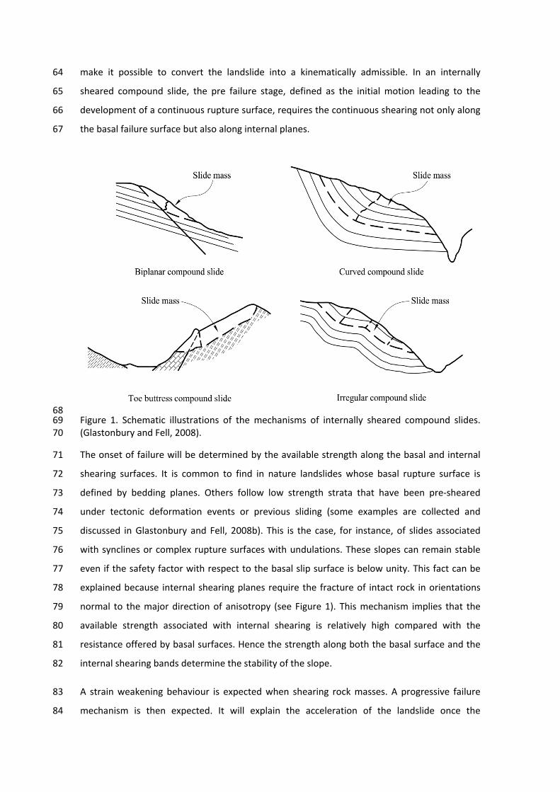
make it possible to convert the landslide into a kinematically admissible. In an internally 64

sheared compound slide, the pre failure stage, defined as the initial motion leading to the 65

development of a continuous rupture surface, requires the continuous shearing not only along 66

the basal failure surface but also along internal planes. 67

68 Figure 1. Schematic illustrations of the mechanisms of internally sheared compound slides. 69 (Glastonbury and Fell, 2008). 70

The onset of failure will be determined by the available strength along the basal and internal 71

shearing surfaces. It is common to find in nature landslides whose basal rupture surface is 72

defined by bedding planes. Others follow low strength strata that have been pre-sheared 73

under tectonic deformation events or previous sliding (some examples are collected and 74

discussed in Glastonbury and Fell, 2008b). This is the case, for instance, of slides associated 75

with synclines or complex rupture surfaces with undulations. These slopes can remain stable 76

even if the safety factor with respect to the basal slip surface is below unity. This fact can be 77

explained because internal shearing planes require the fracture of intact rock in orientations 78

normal to the major direction of anisotropy (see Figure 1). This mechanism implies that the 79

available strength associated with internal shearing is relatively high compared with the 80

resistance offered by basal surfaces. Hence the strength along both the basal surface and the 81

internal shearing bands determine the stability of the slope. 82

A strain weakening behaviour is expected when shearing rock masses. A progressive failure 83

mechanism is then expected. It will explain the acceleration of the landslide once the 84

kinematically admissible mechanism is generated and a set of failure surfaces are completely 85

formed. This aspect was also analyzed, in a simple manner, by Alonso et al. (2010) (Chapter 2). 86

The relevant effect of internal shearing and internal brittleness was invoked by Hutchinson 87

(1987) to interpret the response of Vajont slide (Hendron and Patton, 1985). Mencl (1966) also 88

analysed the kinematics of this landslide and proposed different failure mechanisms, in 89

particular the development of a Prandtl’s wedge within the mass. Vajont slide is described as 90

an ancient landslide reactivated due to the combined effect of a reservoir impoundment which 91

submerged part of the slope toe and rainfall infiltration. Two representative cross-sections of 92

Vajont slope are plotted in Figure 2. 93

94 Figure 2. Two representative cross-sections of Vajont landslide: (a) Section 2; (b) Section 5. 95 (After Hendron and Patton, 1985). P1 and P2 indicates the position of and length of 96 piezometers. (Horizontal scale = Vertical scale). 97 98

The valley slope follows the shape of a syncline structure which folded Jurassic and Cretaceous 99

strata. The basal failure surface was located in clayey layers subjected to intense shearing in 100

past geological times because of previous instability. Above the sliding surface, finely stratified 101

layers of marl and limestone from the Mälm period were identified. Given the shape of the 102

basal failure surface the slide movement requires the shearing along internal planes crossing 103

the marl and limestone strata as a result of the sharp transition between the upper and 104

steeper failure surface and the lower and practically horizontal part. 105

Vajont slide movements were correlated with the impounding of the reservoir. During three 106

years, from 1960 to 1963, the reservoir level rose from 580 m a.s.l to 700 m a.s.l. During this 107

period of time about 4 m of surface displacement were accumulated (Nonveiller, 1987). The 108

increase of the reservoir level up to 700 m led to a violent and accelerated failure. The Vajont 109

slide behaviour was interpreted by Hutchinson (1987, 1994) who included the effect of 110

internal shearing planes. Consider in Figure 3, the critical stability condition of Vajont slope 111

when the reservoir water level rose to an elevation of about 600 m a.s.l. Under this condition a 112

safety factor equal to 1 can be formally assigned within the context of overall limit equilibrium. 113

The increase of the reservoir level (from 600 m a.s.l. to 700 m a.s.l.) resulted in a pore pressure 114

build-up and a reduction of the effective shearing strength along the basal plane surface. As a 115

result a progressive increment of the mobilized shearing strength along the internal shearing 116

planes crossing the rock mass is expected in order to maintain equilibrium. Taking into account 117

the brittleness of the Cretaceous limestones and marly limestones, the internal shearing 118

strength will be progressively mobilized. But this process has a limit. Continuous internal 119

shearing planes will eventually develop and a kinematically admissible mechanism will be 120

formed. According to Figure 3, at this moment the safety factor drops suddenly. This time 121

instant marks the sudden acceleration of the sliding mass. 122

123 Figure 3. Approximate variation of the safety factor with rising reservoir level showing the 124 internal breaking effect and the sudden acceleration resulting from brittle failure on internal 125 shears (from Hutchinson, 1987). 126

127

The post failure behavior in the case of internally sheared compound landslides, in general, 128

and in the case of Vajont, in particular, should be analyzed as a new stage of dynamic 129

deformation. Once the residual strength is reached along the most stressed internal shearing 130

planes and the slide accelerates and moves forward, “new” material from the upper wedge 131

having an available strength higher than the residual one, because it has not been mobilized 132

yet, should be sheared in order to fulfill the kinematic conditions of the motion. This stage will 133

be included in the analysis, as well as the new sliding geometry which is continuously evolving 134

with the motion. 135

The objective of this paper is to analyze the relevance of internal kinematics and the internal 136

degradation of the sliding mass through an appropriate computational tool capable of 137

describing the landslide motion including the onset of the failure and the runout in the case of 138

a brittle (strain-softening) rock. The Material Point Method (MPM) (Sulsky et al., 1994) has 139

been selected as an appropriate computational technique because it is able to simulate large 140

displacements in a dynamic context. The continuum is discretized by means of a set of 141

lagrangian material points. MPM permits combining geological, geometrical, hydraulic, and 142

geotechnical features in order to understand the stability of the slide. Moreover, the dynamic 143

formulation allows the analysis of the kinematics of the motion and modeling, in a unified 144

calculation, the failure and the post-failure behaviour. Similarly to the work presented by 145

Zabala &Alonso (2011), the brittleness of the material will be simulated by means of an 146

elastoplastic constitutive model which includes strain softening. 147

The analysis presented in this paper refers to a particular case which is inspired in Vajont 148

landslide. The landslide is triggered by increasing the pore water pressure inside the slope. 149

Before discussing the results obtained, the computational model, details of the analysis and 150

limitations are described. The evolution of the slope deformation during the pre-failure stage 151

and the post-failure response up to the stabilization of the landslide is described. 152

Vajont landslide was characterized by the high velocity reached, which was estimated to be 153

about 20-30 m/s after 400 m of displacement approximately. These values were estimated 154

according to the height of the generated wave, which reached 235 m above the reservoir level 155

(Hendron & Patton, 1985). Such acceleration can be explained assuming a drop of the basal 156

shear strength to values near zero. The favorite explanation in a number of published 157

contributions on the subject is associated with the development of frictional heat at the sliding 158

surface which induces the increase in water pressure due to the dilation of pore water as 159

temperature increases (Faust, 1982; Hendron and Patton; 1985; Vardoulakis, 2002; Rice, 2006; 160

Veveakis et al., 2007; Goren and Aharonov, 2009; Pinyol and Alonso, 2010a, 2010b; Cecinato et 161

al., 2011; Cecinato and Zervos, 2012). In some contributions heat induced soil plastic collapse 162

of the shearing band is also included in the formulation. 163

The loss of strength available on the basal failure surface will also be introduced in the analysis 164

presented here. The objective was to calculate the slide run-out and maximum velocity and to 165

compare it with field behaviour. Unlike previous contributions the analysis performed include 166

a massive internal shearing in a brittle rock during the entire motion of the slide, which implies 167

major changes in geometry. The initial and final geometry of Vajont landslide is plotted in 168

Figure 4. The mass crossed the valley and climbed up the opposite slope. This stage of the slide 169

resulted also in internal rock shearing which was incorporated into the analysis. 170

Analyses of Vajont were recently reported by Crosta et al. (2015) and Zhao et al. (2015). The 171

first paper presents a FE modelling of the landslide motion (2D and 3D) adopting an arbitrary 172

Eulerian-Lagrangian method. The second paper represents the sliding mass by a Distinct 173

Element model. They pay special attention to the generation of impulse waves in the reservoir. 174

175 Figure 4. Cross sections (a) before and (b) after the landslide (from Del Ventisette, 2015; 176 modified after Rossi and Semenza, 1965). (Horizontal scale = Vertical scale). 177

2. Outline of the MPM method 178

The Material Point Method (MPM) was originally developed by Sulsky et al. (1994). It is 179

typically classified as a method in between the mesh-free methods and the classical Finite 180

Element Method (FEM). MPM discretises the continuum by means of a set of lagrangian 181

points, so-called material points. Each point represents a subdomain of the media and carries 182

all the information (e.g. mass, volume, position, velocity, strain, stress). Besides, governing 183

motion equations are solved incrementally at the nodes of a background computational mesh 184

which remains fixed throughout the calculation and covers the full domain of the problem. The 185

standard nodal interpolation functions provide the relationship between material points and 186

the grid at every time step. This dual description of the domain avoids mesh tangling and 187

allows the simulation of large displacements without re-meshing. Moreover, the detection of 188

contact between different bodies is automatic and the implementation of specific contact 189

elements is not required. A scheme of the spatial discretization used in MPM is illustrated in 190

Figure 5. 191

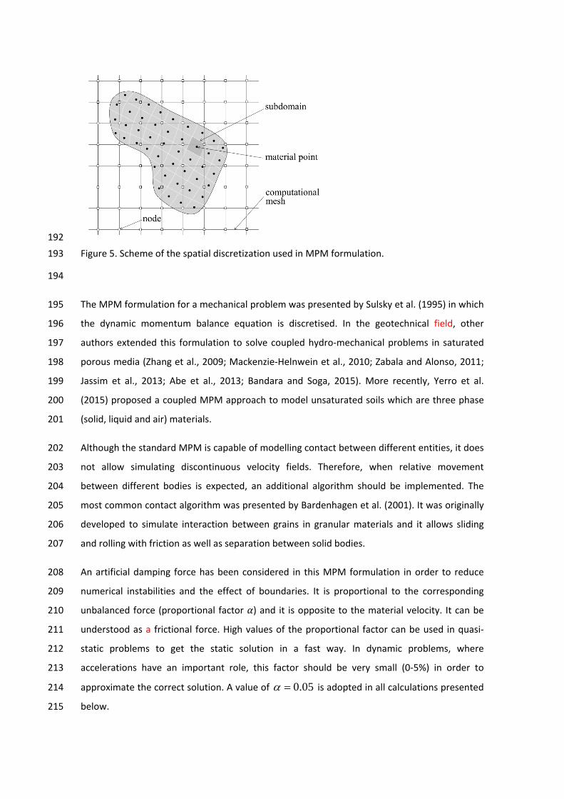
192 Figure 5. Scheme of the spatial discretization used in MPM formulation. 193

194

The MPM formulation for a mechanical problem was presented by Sulsky et al. (1995) in which 195

the dynamic momentum balance equation is discretised. In the geotechnical field, other 196

authors extended this formulation to solve coupled hydro-mechanical problems in saturated 197

porous media (Zhang et al., 2009; Mackenzie-Helnwein et al., 2010; Zabala and Alonso, 2011; 198

Jassim et al., 2013; Abe et al., 2013; Bandara and Soga, 2015). More recently, Yerro et al. 199

(2015) proposed a coupled MPM approach to model unsaturated soils which are three phase 200

(solid, liquid and air) materials. 201

Although the standard MPM is capable of modelling contact between different entities, it does 202

not allow simulating discontinuous velocity fields. Therefore, when relative movement 203

between different bodies is expected, an additional algorithm should be implemented. The 204

most common contact algorithm was presented by Bardenhagen et al. (2001). It was originally 205

developed to simulate interaction between grains in granular materials and it allows sliding 206

and rolling with friction as well as separation between solid bodies. 207

An artificial damping force has been considered in this MPM formulation in order to reduce 208

numerical instabilities and the effect of boundaries. It is proportional to the corresponding 209

unbalanced force (proportional factor 𝛼𝛼) and it is opposite to the material velocity. It can be 210

understood as a frictional force. High values of the proportional factor can be used in quasi-211

static problems to get the static solution in a fast way. In dynamic problems, where 212

accelerations have an important role, this factor should be very small (0-5%) in order to 213

approximate the correct solution. A value of 0.05α = is adopted in all calculations presented 214

below. 215

3. Brittle Mohr-Coulomb model 216

Because MPM is based on continuum mechanics, the constitutive behaviour of the material 217

can be formulated within the theory of elasto-plasticity. In this work, an elastoplastic Mohr-218

Coulomb constitutive model with strain softening has been implemented to simulate the 219

brittleness of rock masses (Yerro et al., 2014). In order to reduce the singularities of the Mohr-220

Coulomb yield surface, the modifications proposed by Abbo and Sloan (1995) have been 221

introduced. An explicit sub-stepping algorithm with error control and a correction for the yield 222

surface drift have been applied (Potts and Gens, 1985) . 223

Softening rules describe how the strength parameters vary with plastic straining. In this case, 224

the state parameters are cohesion c′ and friction angle ϕ′ which decrease exponentially with 225

the accumulated deviatoric plastic stain invariant pdε as: 226

( ) pd

r p rc c c c e ηε−′ ′ ′ ′= + − (1) 227

( ) pd

r p r e ηεϕ ϕ ϕ ϕ −′ ′ ′ ′= + − (2) 228

The deviatoric plastic stain invariant pdε is defined as follows 229

23

p p pd ij ijε = e e (3) 230

where pije is the deviatoric part of the plastic strain tensor. 231

The model requires the specification of peak ( ),p pc ϕ′ ′ and residual ( ),r rc ϕ′ ′ strength 232

parameters. The rate of strength decrease is essentially controlled by the plastic shear strain 233

but an additional “shape factor” parameterη is also included in equations (1) and (2). The 234

higher the shape factorη , the smaller the loss in strength. 235

The inclusion of strain-softening features in continuum numerical methods leads to strain-236

localization problems. In order to reduce the mesh dependence associated with this 237

phenomenon, Rots et al (1985) describe a smeared crack approach as a suitable regularization 238

technique. It postulates that the total work dissipated by a shear band is equivalent to the 239

fracture energy dissipated in a theoretical discrete crack. Then, assuming that the thickness of 240

a shear band is approximately the size of mesh elements, the parameter η can be calibrated 241

by performing a set of numerical simple shear tests. An acceptable relationship of shear stress-242

displacement provides a value of η for a certain element size. This process has also been 243

recently described in Soga et al. (2015). 244

4. Description of the MPM model 245

Geometry and numerical parameters 246

The model presented in this work (Figure 6) is inspired in a simplified geometry of the Vajont 247

slope but close to the real one (section 5 in Figure 2b). It is based on a representative cross-248

section of the valley located 600 m upstream of the dam position (Hendron and Patton, 1987). 249

The geometry of the problem consists of a rock mass volume lying above a pre-existing basal 250

sliding surface (Figure 6). Below the sliding surface the material remained unaffected hence it 251

is not included in the model. 252

In 1960, after the dam was built and the reservoir partially impounded, some field 253

observations revealed the existence of a peripheral crack (Belloni and Stefani, 1987). This 254

continuous crack was an indication that a huge rock mass was partially detached from the rest 255

of the slope. 256

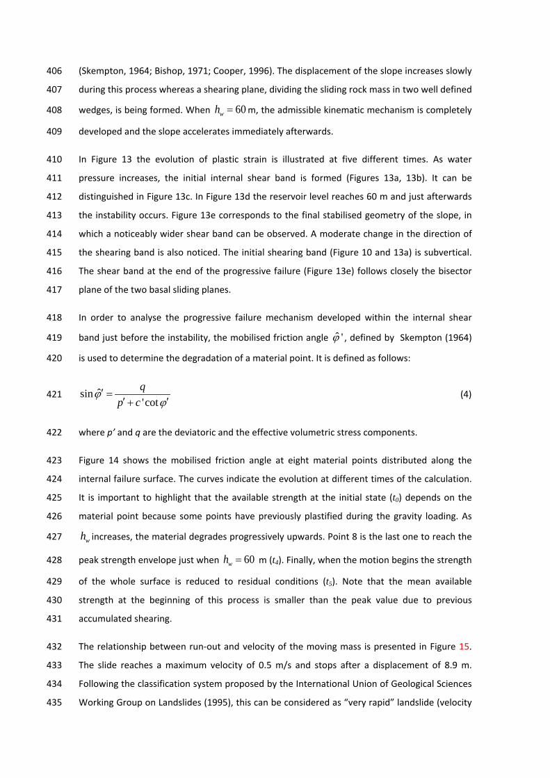
The model presented in this work is a thin slice, 20 m wide, made of 4609 tetrahedral 257

elements. All nodes of the computational mesh are contained within the two slice faces. In this 258

way, a plane strain modelling is carried out restraining to zero the perpendicular movement to 259

the slice faces. 260

Figure 7 illustrates the initial distribution of the material points representing the rock mass 261

above the sliding surface. The computational mesh defines the whole domain of the problem. 262

Four material points are initially distributed within the fully filled elements. These are located 263

at the corresponding integration points of a 4-point Gaussian quadrature. The mean edge 264

element size where the failure is expected is 20 m. 265

Although the relationship between reservoir level and slide velocity was not entirely clear, it 266

seemed evident that the reservoir filling was the determining triggering mechanism of the 267

Vajont landslide. In fact, the groundwater conditions are poorly known. Only the 268

measurements of a few piezometers distributed along the slide (Figure 2) were available 269

(Hendron and Patton, 1987, based on data from Müller, 1964). Probably, the water pressures 270

that really controlled the stability of the slope were those prevailing at the sliding surface, but 271

none of the piezometers was deep enough to reach it. 272

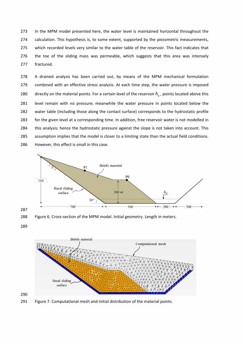
In the MPM model presented here, the water level is maintained horizontal throughout the 273

calculation. This hypothesis is, to some extent, supported by the piezometric measurements, 274

which recorded levels very similar to the water table of the reservoir. This fact indicates that 275

the toe of the sliding mass was permeable, which suggests that this area was intensely 276

fractured. 277

A drained analysis has been carried out, by means of the MPM mechanical formulation 278

combined with an effective stress analysis. At each time step, the water pressure is imposed 279

directly on the material points. For a certain level of the reservoir wh , points located above this 280

level remain with no pressure; meanwhile the water pressure in points located below the 281

water table (including those along the contact surface) corresponds to the hydrostatic profile 282

for the given level at a corresponding time. In addition, free reservoir water is not modelled in 283

this analysis; hence the hydrostatic pressure against the slope is not taken into account. This 284

assumption implies that the model is closer to a limiting state than the actual field conditions. 285

However, this effect is small in this case. 286

287 Figure 6. Cross-section of the MPM model. Initial geometry. Length in meters. 288

289

290 Figure 7. Computational mesh and initial distribution of the material points. 291

Kinematic constrains of the model 292

Alonso et al. (2010) analysed the kinematics of Vajont slide. They assumed that all points slid 293

parallel to the basal failure surface with the same absolute velocity. In advanced stages of the 294

post-failure, the motion of the slide implies that mass from the upper wedge becomes part of 295

the lower one (Figure 8). During this process, the lower sliding surface accumulates shearing 296

strains. On the other hand, the rock mass arriving to the position of the internal shearing band 297

becomes sheared to a certain extent and moves downhill leaving intact the rock upslope (as 298

indicated in Figure 8). According to this scenario, the internal shearing band receives 299

continuously new undisturbed rock as the slide moves downhill. Shearing along the internal 300

shearing band will result in a process of progressive failure which, in an extreme case, will take 301

the rock to residual conditions. 302

The model presented below will clarify if these assumptions are consistent with the brittle 303

constitutive model of the rock material and the overall geometrical dynamic evolution of the 304

motion. 305

306 Figure 8. Kinematics of sliding. Two-block mechanism and internal rock degradation (a case of 307 compound landslide in a brittle material). 308

Materials and initial state 309

Vajont rockslide was, in fact, the reactivation of a paleolandslide. Semenza (2001) attempted 310

to reconstruct the past history of the slide and he came up with a set of cross-sections 311

illustrating a possible sequence of events. He interpreted that erosion processes at the toe of 312

the slope caused by the Vajont river could explain the initiation of the failure surface and the 313

past motion of the slope. Figure 9 illustrates a simplified reconstruction of the paleolandslide. 314

During the deformation process the slope was subjected to cumulative relative displacements 315

and intense fracturing, because of the kinematic constraints imposed by the kink of the sliding 316

surface. Because the rock strength depends on the deformation history, it could be expected 317

that, at the time of the dam construction, some areas could already be damaged. 318

319 Figure 9. Simplified reconstruction of the paleolandslide: (a) original profile; (b) profile after 320 paleolandslide; (c) initial profile for the present analysis after erosion of the toe. 321

The nature of the Vajont sliding surface was discussed by Hendron and Patton (1985). They 322

concluded that it was a layer of a few centimetres thick of high plasticity clay. Taking into 323

account the scale of the whole problem (the final displacement of the slope was several 324

hundred meters) the thickness of the shear band is neglected in this work. A contact algorithm 325

proposed by Bardenhagen et al. (2001) and implemented by Al-Kafaji (2013) is used to model 326

the basal sliding surface. This is a frictional contact in which the slip occurs when the tangential 327

force exceeds the maximum allowable threshold determined by Coulomb friction. 328

Considering the past history of the landslide it is clear that the residual friction angle of the 329

clay layers was the most relevant parameter controlling the strength of the basal sliding 330

surface. Most of the early Vajont stability analyses concentrated on determining the basal 331

sliding strength necessary to maintain the equilibrium of the slope (Mencl, 1966; Skempton, 332

1966; Kenney, 1967). Some of them are based on classic limit equilibrium methods (LEM) in 333

which the basal stability angle ( bϕ′ ) was estimated in the range of 18-28º. These values are not 334

consistent with laboratory tests. Some authors (Hendron and Patton, 1985; Tika and 335

Hutchinson, 1999) examined the shearing strength by direct and ring shear tests on clay 336

samples from the basal sliding surface and estimated that the static residual friction angle was 337

around 10ºb′ =ϕ . Hendron and Patton (1985) suggested that the roughness of the failure 338

surface could amount to two additional degrees and proposed 12ºbϕ′ = as a suitable choice. 339

In this analysis 12ºbϕ′ = has been used in the contact algorithm. 340

Above the basal sliding surface, marls layers were identified. Lying above marls, there were 341

limestone strata (Semenza, 2001). In this model, a unique rock material has been used to 342

simulate the whole rock volume. Following Hoek (2007), Alonso et al. (2010) approximated the 343

strength envelope of the material above the sliding surface. The effective Mohr-Coulomb 344

strength parameters were determined for a range of normal stresses of 2 MPa ( 787c′ = kPa 345

and 38.5ºϕ′ = ). They also analysed the static equilibrium of the slide by using a simple two-346

block model and suggested a range of effective strength values. These strength parameters are 347

rough average approximations. 348

Rock material is typically characterised by brittle behaviour. In this work the Mohr-Coulomb 349

peak envelope is defined by the strength parameters 1900pc′ = kPa and 42ºpϕ′ = ; the residual 350

strength of the rock is defined by 300rc′ = kPa and 36ºrϕ′ = . The shape factor adopted to 351

control the rate of strength decrease is 150η = . Other material parameters are summarized in 352

Table 1. Even if there are uncertainties on an appropriate set of average “in situ” parameters 353

(Superchi, 2012), the selected set offers a good approximation to discuss the effect of internal 354

degradation of the material during the landslide motion. 355

Table 1. Material parameters of rock mass. 356

Material parameter Value

Porosity, n 0.2

Young Modulus, E [GPa] 5

Poisson ratio, ν 0.33

Solid density, ρ [kg/m3] 2700

Peak effective cohesion, pc′ [kPa] 1900

Residual effective cohesion, rc′ [kPa] 300

Peak effective friction angle, pϕ′ [ º ] 42

Residual effective friction angle, rϕ′ [ º ] 36

Shape factor, η 150

357

Reproducing the initial stress state in the field is a difficult task in the absence of data. 358

However, trying to exactly reproduce the processes that have affected the rock mass during its 359

past geological history is out of the scope of this work. In this analysis, a gravity loading has 360

been applied to the intact material in order to calculate an initial stress state. It seemed 361

reasonable to consider the rock weight as the most relevant factor to determine the initial 362

stress state in the slope. 363

In the model presented below, a gradual gravity loading is applied to the intact material. As a 364

result, some points above the kink are sheared, accumulating plastic strain and a two-block 365

kinematically admissible mechanism is initiated. The strength is reduced locally along this 366

“initial” internal shear band and its mean value becomes intermediate between peak and 367

residual states (Figure 10). Finally, a stable geometry is obtained. During this process, the level 368

of the reservoir is maintained at the position of the horizontal lower basal sliding surface ( wh = 369

0 m). As a consequence, the rock located within the current internal shear band damages 370

according to the brittleness of the material. 371

Because the paleolandslide was not simulated, the toe of the slope remains under peak 372

conditions. The stability of a compound slide is essentially controlled by the strength of both 373

the basal surface and the internal shearing band. Therefore, the strength of the rock mass that 374

has already been sheared at the kink does not play a significant role in the stability of the 375

slope. 376

Figure 10 shows the accumulated deviatoric plastic strain after gravity loading. It is localised 377

along an almost vertical band that initiates at the existing kink of the basal surface and 378

progresses a significant distance upwards. 379

380 Figure 10. Scheme of deviatoric plastic strain field under gravity loading (initial state). 381

5. Numerical results 382

Dynamic behaviour and internal degradation of rock mass 383

According to Hendron and Patton (1985) and Hutchinson (1987) (Figure 3), Vajont slide 384

reached critical stability conditions when the reservoir water level was about 20 m above the 385

lowest level of the slide toe. However, surface measurements indicated an accelerated 386

movement, for the first time, when the water level was around 60 m. Immediately afterwards, 387

the reservoir was partially emptied in order to stabilise the slope. Later on, the reservoir level 388

was increased and decreased again. Finally, the fast landslide occurred when the reservoir 389

elevation was about 120 m. 390

In this work, only an initial increase of the water level (60 m) has been simulated and no 391

further decrease of reservoir elevation has been considered. For this reason, the reservoir level 392

was maintained at 60 m. In the model presented here, the water level is increased in intervals 393

of 10 m up to failure (Figure 11). Afterwards, it is maintained constant thereafter until 394

stabilisation of the motion. 395

The movement of point P0 (Figure 6) is illustrated in Figure 12. Note that the displacement is in 396

meters and the scale is logarithmic. As the water pressures increase within the slope, P0 is 397

stable. When the water level reaches a value of 60 m, the displacement of P0 increases rapidly 398

leading to a final movement of 8.5 m. In the same figure, the movement of point P1, located at 399

the upper sliding wedge, is also represented. It is clear that both points (P0 and P1) displace 400

the same amount, which supports the kinematic hypothesis suggested by Alonso et al. (2010). 401

Water level rise causes a reduction of the mean effective stresses within the slope, leading 402

more points to reach the yield function envelope. The strain softening behaviour reduces the 403

available strength and the progressive internal degradation of the rock mass continues. This 404

mechanism was identified as a progressive failure phenomenon by early contributions 405

(Skempton, 1964; Bishop, 1971; Cooper, 1996). The displacement of the slope increases slowly 406

during this process whereas a shearing plane, dividing the sliding rock mass in two well defined 407

wedges, is being formed. When 60wh = m, the admissible kinematic mechanism is completely 408

developed and the slope accelerates immediately afterwards. 409

In Figure 13 the evolution of plastic strain is illustrated at five different times. As water 410

pressure increases, the initial internal shear band is formed (Figures 13a, 13b). It can be 411

distinguished in Figure 13c. In Figure 13d the reservoir level reaches 60 m and just afterwards 412

the instability occurs. Figure 13e corresponds to the final stabilised geometry of the slope, in 413

which a noticeably wider shear band can be observed. A moderate change in the direction of 414

the shearing band is also noticed. The initial shearing band (Figure 10 and 13a) is subvertical. 415

The shear band at the end of the progressive failure (Figure 13e) follows closely the bisector 416

plane of the two basal sliding planes. 417

In order to analyse the progressive failure mechanism developed within the internal shear 418

band just before the instability, the mobilised friction angle ˆ 'ϕ , defined by Skempton (1964) 419

is used to determine the degradation of a material point. It is defined as follows: 420

ˆsin'cotq

p cϕ

ϕ′ =

′ ′+ (4) 421

where p’ and q are the deviatoric and the effective volumetric stress components. 422

Figure 14 shows the mobilised friction angle at eight material points distributed along the 423

internal failure surface. The curves indicate the evolution at different times of the calculation. 424

It is important to highlight that the available strength at the initial state (t0) depends on the 425

material point because some points have previously plastified during the gravity loading. As 426

wh increases, the material degrades progressively upwards. Point 8 is the last one to reach the 427

peak strength envelope just when 60wh = m (t4). Finally, when the motion begins the strength 428

of the whole surface is reduced to residual conditions (t5). Note that the mean available 429

strength at the beginning of this process is smaller than the peak value due to previous 430

accumulated shearing. 431

The relationship between run-out and velocity of the moving mass is presented in Figure 15. 432

The slide reaches a maximum velocity of 0.5 m/s and stops after a displacement of 8.9 m. 433

Following the classification system proposed by the International Union of Geological Sciences 434

Working Group on Landslides (1995), this can be considered as “very rapid” landslide (velocity 435

limits: 0.05-5 m/s). The calculated run-out-velocity relationship is very similar to the 436

relationship calculated by Alonso et al. (2010) in which the dynamic motion equation for two 437

interacting wedges was solved. 438

439 Figure 11. Water table evolution. 440

441

442 Figure 12. Run out of the slide. Variation of absolute displacements of points P0 and P1, in 443 terms of reservoir water level. 444

445

446 (a) 447

448 (b) 449

450 (c) 451

452

(d) 453

454

(e) 455

Figure 13. Contours of deviatoric plastic strain at different positions of the water level. (a) 456

50wh = m; (b) 54wh = m; (c) 57wh = m; (d) 60wh = m; (e) final stable geometry. 457

458 Figure 14. Progressive failure. Evolution of mobilised friction angle along the internal shear 459 band at different times (in terms of water level): (t0) initial state; (t1) 20wh = m; (t2) 40wh = m; 460

(t3) 50wh = m; (t4) 57wh = m; (t5) 60wh = m. 461

462 Figure 15. Calculated run-out and slide velocity of point P0. 463

464

Reduction of basal surface friction angle 465

Vajont slide moved forward approximately 450 m in a few seconds, reaching an estimated 466

velocity of 20-30 m/s (Hendron and Patton, 1985), which is an “extremely rapid” motion. A 467

relevant question in Vajont landslide is why the sliding mass accelerated so much. The 468

maximum speed in the model discussed in the previous section is about two orders of 469

magnitude lower, despite the effort to reproduce the real case. 470

Authors tried to explain the increase in speed in different ways. One of them is the effect of 471

strain rate on clay friction. Tika and Hutchinson (1999) tested at different strain rates 472

remoulded specimens from clay layers belonging to the sliding surface. They found that 473

friction angle decreases with strain rate and they reported minimum residual values of 474

5ºbϕ′ = . Many authors have reported in recent years the results of high velocity shearing 475

(limited to around 1.3 m/s in most cases) in a variety of soil types (Di Toro et al, 2006; 476

Mizoguchi et al, 2007; Liao et al 2011; Han and Hirose, 2012; Yang et al, 2014) tested both 477

saturated and unsaturated as well as in samples from Vajont weak layers (Ferri et al, 2010). 478

The change in friction angle with shearing rates is however a controversial issue discussed in 479

some detail in Alonso et al. (2015). 480

The most accepted explanation for the extremely high sliding velocity is associated with the 481

development of frictional heat at the basal sliding surface (Uriel Romero & Molina, 1977; Voigt 482

and Faust, 1982; Nonveiller, 1987; Vardoulakis, 2002; Pinyol & Alonso, 2010). The initiation of 483

the movement and the frictional work input on the sliding shearing band results in an increase 484

in temperature. Then, water pressure within the clayey band increases and the available 485

effective stress along the basal sliding surface is reduced to near-zero values and shearing 486

strength vanishes (which is equivalent to the condition 0ºbϕ′ ≈ ). 487

In order to analyze the effect of the basal strength on the sliding speed two additional 488

calculations have been carried out. Starting at the stabilized geometry (described in the 489

previous section), and maintaining the water level at 60wh = m, the effective friction angle 490

imposed along the basal contact surface was reduced from 12ºbϕ′ = to 5ºbϕ′ = in the first 491

calculation, and to 0ºbϕ′ = in the second one. 492

Figure 16 shows the results for the two analyses. The evolution of the accumulated deviatoric 493

plastic strain is presented. The two slides accelerate immediately after the reduction of the 494

basal contact strength. Mass from the active wedge enters into the internal shearing zone. 495

Strength in the band reduces due to the brittle behaviour of the rock and, this degraded mass 496

becomes part of the passive wedge as the motion proceeds. When the mobilised mass reaches 497

the opposite side of the valley another shearing zone is developed at the position of the kink of 498

the basal surface. Now, the toe of the slope, which until now has remained at peak strength, is 499

sheared as it climbs the slope. The smaller the basal strength, the longer the upward 500

displacement of the rock mass before getting a new stable geometry. 501

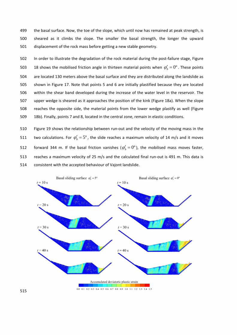
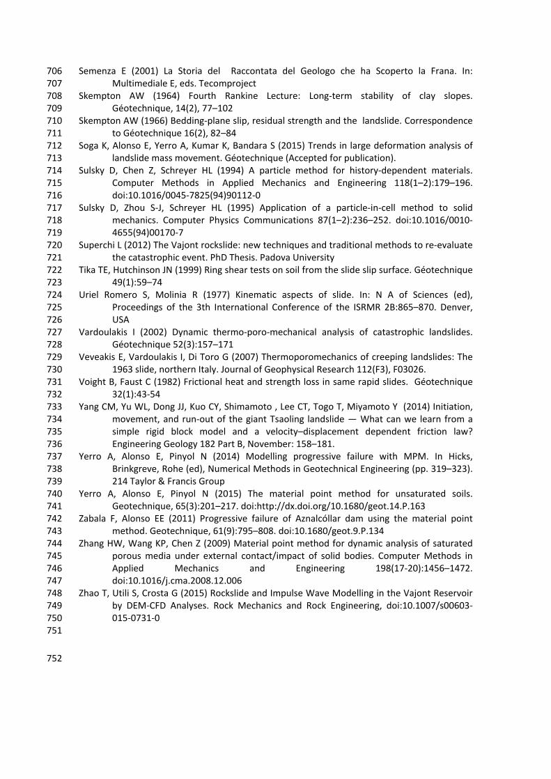
In order to illustrate the degradation of the rock material during the post-failure stage, Figure 502

18 shows the mobilised friction angle in thirteen material points when 0ºbϕ′ = . These points 503

are located 130 meters above the basal surface and they are distributed along the landslide as 504

shown in Figure 17. Note that points 5 and 6 are initially plastified because they are located 505

within the shear band developed during the increase of the water level in the reservoir. The 506

upper wedge is sheared as it approaches the position of the kink (Figure 18a). When the slope 507

reaches the opposite side, the material points from the lower wedge plastify as well (Figure 508

18b). Finally, points 7 and 8, located in the central zone, remain in elastic conditions. 509

Figure 19 shows the relationship between run-out and the velocity of the moving mass in the 510

two calculations. For 5ºbϕ′ = , the slide reaches a maximum velocity of 14 m/s and it moves 511

forward 344 m. If the basal friction vanishes ( 0ºbϕ′ = ), the mobilised mass moves faster, 512

reaches a maximum velocity of 25 m/s and the calculated final run-out is 491 m. This data is 513

consistent with the accepted behaviour of Vajont landslide. 514

515

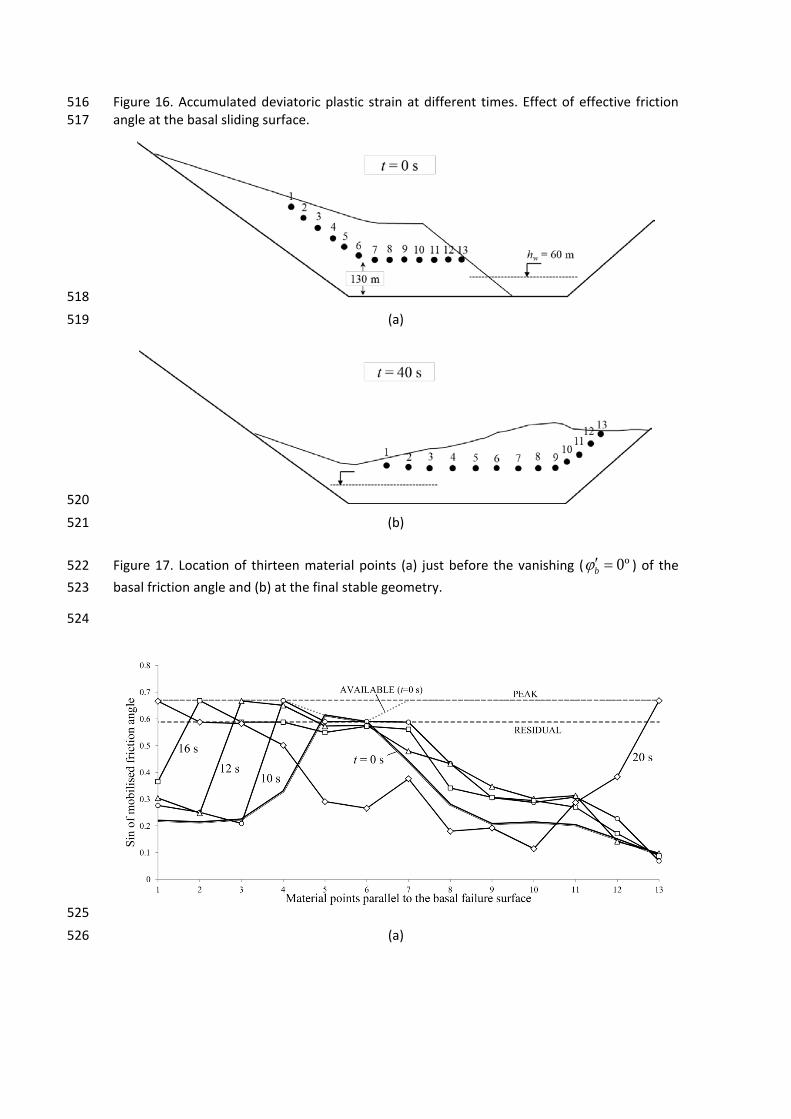
Figure 16. Accumulated deviatoric plastic strain at different times. Effect of effective friction 516 angle at the basal sliding surface. 517

518 (a) 519

520 (b) 521

Figure 17. Location of thirteen material points (a) just before the vanishing ( 0ºbϕ′ = ) of the 522 basal friction angle and (b) at the final stable geometry. 523

524

525 (a) 526

527 (b) 528

Figure 18. Rock degradation for 0ºbϕ′ = . Evolution of mobilised friction angle at thirteen 529 material points distributed along the slope, parallel to the basal failure surface (indicated in 530 Figure 17). (a) Initial degradation of the upper wedge; (b) toe degradation. 531

532 Figure 19. Calculated run-outs and sliding velocity. Effect of friction angle at the basal sliding 533 surface. 534

6. Discussion 535

The model presented above is a simplification of the Vajont compound slide in which a sharp 536

transition between the inclined upper planar sliding surface and the horizontal lower one has 537

been considered. According to Semenza (2001), the actual transition between the two fairly 538

planar surfaces was probably more rounded (see Figure 4a). This modified geometry could, “a 539

priori” have a significant impact on the results, especially as far as the failure mechanism is 540

concerned. In order to study this effect an additional calculation incorporating a more realistic 541

geometry has been carried out. A circular arc having a 200 m radius (R=200m) substitutes the 542

previous sharp kink and characterises now the fold of the new sliding surface. It reproduces in 543

a satisfactory manner Figure 2b. Rock properties, gravity loading, and the trigger of instability 544

did not change with respect to the previous model. 545

The new basal failure surface is shown in Figure 20. Also shown in the figure are the 546

distribution of plastic shearing strains when the slope was made unstable by reducing the 547

basal friction angle to 0ºbϕ′ = . The plot corresponds to a time t= ...s after the initiation of the 548

motion. Unlike the previous single internal shearing band starting at the kink (Figure 13), two 549

shearing planes progress from the fold towards the surface of the slope defining a sector-550

shaped area (Figure 20), leading to a wider and irregular shearing zone. 551

The relationship between run-out and velocity for the new analysis is given in Figure 21. The 552

maximum velocity and run-out obtained are slightly higher than the results obtained 553

previously with the simplified sharp geometry (Figure 19). For 0ºbϕ′ = the calculated 554

maximum velocity is now close 27 m/s and the maximum run-out is 503 m. These figures could 555

be compared with the equivalent values for the sharp geometry (25 m/s and 491 m 556

respectively). If the basal friction is reduced to 5ºbϕ′ = in the rounded case these values are 557

17 m/s and 384 m, against 14 m/s and 344 m for the sharp geometry. Results are similar. Even 558

if a rounded more realistic basal surface is introduced, the estimated velocity and run-out of 559

Vajont landslide requires the cancellation of the basal friction. 560

It is concluded that the rounded geometry introduces a change on the internal failure mode 561

which is probably a more realistic result. However, the essential kinematics of the motion are 562

very similar to the calculated single internal shearing plane developing for the simplified 563

geometry (Figures 7 and 8). Differences between maximum velocity and run-out are 564

considered minor. 565

566

567 Figure 20. Failure mechanism for a rounded basal sliding surface. 568

569 Figure 21. Calculated run-outs and sliding velocity considering a rounded basal sliding surface. 570 Effect of friction angle at the basal sliding surface. 571

7. Conclusions 572

The paper provides some insight into the role of internal shearing to explain the motion of 573

compound landslides. The analysed example, directly based on Vajont geometry, is typical of 574

an initial syncline folding of strata followed by river erosion. In cases of reactivation of previous 575

instability, internal shearing plays a key role to stabilize the impending motion. The limit is the 576

exhaustion of the strength in a shearing area. If the material involved is brittle, the internal 577

failure results in a progressive failure mechanism. 578

In the example presented, the internal failure process is complex because the initial 579

equilibrium state resulted in some post-peak strain softening at a few locations. Further 580

loading (in our case controlled by a rise in water level) resulted in a progressive failure which 581

essentially evolved from the “kink” (sharp or rounded) defined by the geometry of the basal 582

slip surface towards the surface of the slope. Once the last point resisting under peak 583

conditions in the internal shear band advances into strain softening, the failure mechanism 584

becomes kinematically admissible. Afterwards, the slide acceleration begins. 585

An interesting outcome of the analysis presented is that the resulting kinematic mechanism for 586

the sharp kink of the basal surface is essentially defined by a single localization plane which, 587

after some displacement, can be approximately defined as the bisector of the two planes 588

defining the basal sliding surface. This outcome was not obvious because many kinematic 589

mechanisms may explain the motion of the geometry analysed. However, details of the 590

precise continuity and irregularities of the sliding plane will most likely control the geometry of 591

the kinematic mechanism and the position, orientation and number of internal shearing 592

surfaces. This comment was also illustrated in the paper when a more realistic rounded basal 593

sliding surface was analyzed. In this case, two distinct internal shearing surfaces develop in the 594

rock mass. 595

The calculated thickness of the internal shearing planes was significant (20-50m) but this result 596

may be a consequence of the size of elements of the computational mesh. Note also that the 597

rock was discretised as a homogeneous elastoplastic brittle material with no internal structure: 598

bedding planes and fractures. They could play a significant role in the development of 599

kinematic mechanisms. The computational method (MPM), inherently dynamic, provides 600

interesting information on the post-failure motion of the slide. Velocity and run-out are 601

calculated, as well as the evolving geometry during the motion. 602

There was a special interest in checking if the known velocity and run-out of Vajont landslide 603

could be simulated by a combination of internal rock brittleness and a non-zero friction angle 604

at the sliding surface. In fact, a number of previous analyses which rely on thermal 605

pressurization along the basal sliding surface indicated that a zero shear strength was required 606

to reproduce the actual observation. The present contribution confirms that this is the case, 607

even if a significant brittleness is assigned to the internal shearing and even if the kinematic 608

sliding mechanism is simulated with a reasonable accuracy. 609

610

Acknowledgments 611

The authors acknowledge the support provided by the PARTING (Particle Methods in 612

Geomechanics), project financed by the “Ministerio de Economía y Competividad”, Spanish 613

Government. 614

References 615

Abbo A, Sloan S (1995) A smooth hyperbolic approximation to the Mohr-Coulomb yield 616 criterion. Computers & Structures 54(3):427–441 617

Abe K, Soga K, Bandara S (2013) Material Point Method for Coupled Hydromechanical 618 Problems. Journal of Geotechnical and Geoenvironmental Engineering 140(3):1–16 619

Al-Kafaji IKJ (2013) Formulation of a Dynamic Material Point Method (MPM) for 620 Geomechanical Problems. PhD Thesis. Universität Stuttgart 621

Alonso EE, Pinyol NM, Puzrin AM (2010) Geomechanics of Failures. Advanced Topics. Springer. 622 ISBN 978-90-481-3537-0 623

Alonso EE, Zervos A, Pinyol NM (2015) Thermo-poro-mechanical analysis of landslides: from 624 creeping behaviour to catastrophic failure. Accepted for publication in Geotechnique 625

Bandara S, Soga K (2015) Coupling of soil deformation and pore fluid flow using material point 626 method. Computers and Geotechnics 63(1):199–214 627

Bardenhagen SG, Guilkey JE, Roessig KM, Brackbill JU, Witzel WM (2001) An Improved Contact 628 Algorithm for the Material Point Method and Application to Stress Propagation in 629 Granular Material. Computer Modeling in Engineering and Sciences 2(4):509–522 630

Belloni LG, Stefani R (1987) The Vajont slide: Instrumentation - Past experience and the 631 modern approach. Engineering Geology 24:445–474 632

Bishop A (1971) The influence of progressive failure on the choice of the method of stability 633 analysis. Geotechnique 21:168–172 634

Cecinato F, Zervos A (2012) Influence of thermomechanics in the catastrophic collapse of 635 planar landslides. Canadian Geotechnical Journal 49(2):207–225. doi:10.1139/t11-095 636

Cecinato F, Zervos A, Veveakis E (2011) A thermo-mechanical model for the catastrophic 637 collapse of large landslides. International Journal for Numerical and Analytical 638 Methods in Geomechanics 35:1507-1535. doi:10.1002/nag.963 639

Cooper M (1996) The progressive development of a failure slip surface in over-consolidated 640 clay at Selborne, UK. In: Senneset K, eds. Proc. 7th Int. Symp. on Landslides 2:683–688, 641 Trondheim, Norway. Rotterdam: Balkema, Rotterdam 642

Crosta G, Imposimato S, Roddeman D (2015) Landslide Spreading, Impulse Water Waves and 643 Modelling of the Vajont Rockslide. Rock Mechanics and Rock Engineering. Doi: 644 10.1007/s00603-015-0769-z 645

Del Ventisette C, Gigli G, Bonini M, Corti G, Montanari D, Santoro S, Sani F, Fanti R, Casagli N 646 (2015) Insights from analogue modelling into the deformation mechanism of the 647 landslide. Geomorphology 228(September 1963):52–59. 648 doi:10.1016/j.geomorph.2014.08.024 649

Di Toro G, Hirose T, Nielsen S, Pennacchioni G, Shimamoto T (2006) Natural and experimental 650 evidence of melt lubrication of faults during earthquakes. Science 311, February:647–651 649. 652

653

Ferri F, Di Toro G, Hirose T, Shimamoto T (2010) Evidence of thermal pressurization in high-654 velocity friction experiments on smectite-rich gouges. Terra Nova 22, 5:347–353. 655

Glastonbury J, Fell R (2008a) A decision analysis framework for the assessment of likely post-656 failure velocity of translational and compound natural rock slope landslides. Canadian 657 Geotechnical Journal 45(3):329–350. doi:10.1139/T07-082 658

Glastonbury J, Fell R (2008b) Geotechnical characteristics of large slow, very slow, and 659 extremely slow landslides. Canadian Geotechnical Journal 45(7):984–1005. 660 doi:10.1139/T08-021 661

Goren L, Aharonov E (2009) On the stability of landslides: A thermo-poro-elastic approach. 662 Earth and Planetary Science Letters 277(3-4):365–372. 663

Han R, Hirose T (2012) Clay-clast aggregates in fault gouge: An unequivocal indicator of seismic 664 faulting at shallow depths? Journal of Structural Geology 43, October:92–99. 665

Hendron AJ, Patton FD (1985) The Vajont slide, a geotechnical analysis based on new geologic 666 observations of the failure surface. Technical Report GL-85-5, Washington DC 667

Hendron AJ, Patton FD (1987) The slide. A geotechnical analysis based on new geologic 668 observations of the failure surface. Engineering Geology 24:475-491 669

Hoek E (2007) Practical Rock Engineering. http://www.rocscience.com/hoek/ 670 PracticalRockEngineering.asp 671

Hungr O, Leroueil S, Picarelli L (2014) The Varnes classification of landslide types, an update. 672 Landslides 11(April):167-194. 673

Hutchinson JN (1987) Mechanisms producing large displacements in landslides on pre-existing 674 shears. Memoir of the Geological Society of China 9:175–200 675

Hutchinson JN (1994) Some aspects of the morphological parameters of landslides, with 676 example drawn from Italy and elsewhere. Geologica Romana 30:1-12 677

Jassim I, Stolle D, Vermeer P (2013) Two-�phase dynamic analysis by material point method. 678 International Journal for Numerical and Analytical Methods in Geomechanics 679 37(15):2502–2522. doi:10.1002/nag 680

Kenney TC (1967) Stability of the Vajont valley, discussion of a paper by L. Müller (1964) on the 681 rock slide in the Vajont valley. Rock Mechanics and Engineering Geology 5:10–16 682

Liao CJ, Lee DH, Wu JH, Lai CZ (2011) A new ring-shear device for testing rocks under high 683 normal stress and dynamic conditions. Engineering Geology 122, 1-2:93–105. 684

Mackenzie-Helnwein P, Arduino P, Shin W, Moore JA, Miller GR (2010) Modeling strategies for 685 multiphase drag interactions using the material point method. International Journal 686 for Numerical Methods in Engineering 83(3):295–322 687

Mencl V (1966) Mechanics on landslides with non-circular slip surfaces with special reference 688 to the Slide. Géotechnique 19(4):329–337 689

Mizoguchi K, Hirose T, Shimamoto T, Fukuyama E (2007) Reconstruction of seismic faulting by 690 high-velocity friction experiments: An example of the 1995 Kobe earthquake. 691 Geophysical Research Letters 34, August:2–4. 692

Müller L (1964) The rock slide in the Vajont Valley. Rock Mechanics and Engineering Geology 693 2:148–212 694

Nonveiller E (1987) The Vajont reservoir slope failure. Engineering Geology 24:493–512. 695 Pinyol NM, Alonso EE (2010a) Criteria for rapid sliding II. Engineering Geology 114(3-4):211–696

227 697 Pinyol NM, Alonso EE (2010b) Fast planar slides. A closed-form thermo-hydro-mechanical 698

solution. International Journal for Numerical and Analytical Methods in Geomechanics 699 34:27–52 700

Potts D, Gens A (1985) A critical assessment of methods of correcting for drift from the yield 701 surface in elasto-�plastic finite element analysis. Numerical and Analytical Methods in 702 Geomechanics 9(2):149–159 703

Rots JG, Nauta P, Kuster GMA, Blaauwendraad J (1985) Smeared Crack Approach and Fracture 704 Localization in Concrete. Heron, 30(1):1–48 705

Semenza E (2001) La Storia del Raccontata del Geologo che ha Scoperto la Frana. In: 706 Multimediale E, eds. Tecomproject 707

Skempton AW (1964) Fourth Rankine Lecture: Long-term stability of clay slopes. 708 Géotechnique, 14(2), 77–102 709

Skempton AW (1966) Bedding-plane slip, residual strength and the landslide. Correspondence 710 to Géotechnique 16(2), 82–84 711

Soga K, Alonso E, Yerro A, Kumar K, Bandara S (2015) Trends in large deformation analysis of 712 landslide mass movement. Géotechnique (Accepted for publication). 713

Sulsky D, Chen Z, Schreyer HL (1994) A particle method for history-dependent materials. 714 Computer Methods in Applied Mechanics and Engineering 118(1–2):179–196. 715 doi:10.1016/0045-7825(94)90112-0 716

Sulsky D, Zhou S-J, Schreyer HL (1995) Application of a particle-in-cell method to solid 717 mechanics. Computer Physics Communications 87(1–2):236–252. doi:10.1016/0010-718 4655(94)00170-7 719

Superchi L (2012) The Vajont rockslide: new techniques and traditional methods to re-evaluate 720 the catastrophic event. PhD Thesis. Padova University 721

Tika TE, Hutchinson JN (1999) Ring shear tests on soil from the slide slip surface. Géotechnique 722 49(1):59–74 723

Uriel Romero S, Molinia R (1977) Kinematic aspects of slide. In: N A of Sciences (ed), 724 Proceedings of the 3th International Conference of the ISRMR 2B:865–870. Denver, 725 USA 726

Vardoulakis I (2002) Dynamic thermo-poro-mechanical analysis of catastrophic landslides. 727 Géotechnique 52(3):157–171 728

Veveakis E, Vardoulakis I, Di Toro G (2007) Thermoporomechanics of creeping landslides: The 729 1963 slide, northern Italy. Journal of Geophysical Research 112(F3), F03026. 730

Voight B, Faust C (1982) Frictional heat and strength loss in same rapid slides. Géotechnique 731 32(1):43-54 732

Yang CM, Yu WL, Dong JJ, Kuo CY, Shimamoto , Lee CT, Togo T, Miyamoto Y (2014) Initiation, 733 movement, and run-out of the giant Tsaoling landslide — What can we learn from a 734 simple rigid block model and a velocity–displacement dependent friction law? 735 Engineering Geology 182 Part B, November: 158–181. 736

Yerro A, Alonso E, Pinyol N (2014) Modelling progressive failure with MPM. In Hicks, 737 Brinkgreve, Rohe (ed), Numerical Methods in Geotechnical Engineering (pp. 319–323). 738 214 Taylor & Francis Group 739

Yerro A, Alonso E, Pinyol N (2015) The material point method for unsaturated soils. 740 Geotechnique, 65(3):201–217. doi:http://dx.doi.org/10.1680/geot.14.P.163 741

Zabala F, Alonso EE (2011) Progressive failure of Aznalcóllar dam using the material point 742 method. Geotechnique, 61(9):795–808. doi:10.1680/geot.9.P.134 743

Zhang HW, Wang KP, Chen Z (2009) Material point method for dynamic analysis of saturated 744 porous media under external contact/impact of solid bodies. Computer Methods in 745 Applied Mechanics and Engineering 198(17-20):1456–1472. 746 doi:10.1016/j.cma.2008.12.006 747

Zhao T, Utili S, Crosta G (2015) Rockslide and Impulse Wave Modelling in the Vajont Reservoir 748 by DEM-CFD Analyses. Rock Mechanics and Rock Engineering, doi:10.1007/s00603-749 015-0731-0 750

751

752