Internal Flow Thermal/Fluid Modeling of STS-107 Port Wing in Support of the Columbia Accident Investigation Board

John R. Sharp NASA/ Marshall Space Flight Center

ED26/Thermal and Fluid Systems Group Huntsville, Alabama

Ken Kittredge

NASA/ Marshall Space Flight Center ED26/Thermal and Fluid Systems Group

Huntsville, Alabama

Richard G. Schunk NASA/ Marshall Space Flight Center

ED26/Thermal and Fluid Systems Group Huntsville, Alabama

ABSTRACT: As part of the aero-thermodynamics team supporting the Columbia Accident Investigation Board (CAIB), the Marshall Space Flight Center was asked to perform engineering analyses of internal flows in the port wing. The aero-thermodynamics team was split into internal flow and external flow teams with the support being divided between shorter timeframe engineering methods and more complex computational fluid dynamics. In order to gain a rough “order of magnitude” type of knowledge of the internal flow in the port wing for various breach locations and sizes (as theorized by the CAIB to have caused the Columbia re-entry failure), a bulk venting model was required to input boundary flow rates and pressures to the computational fluid dynamics (CFD) analyses. This paper summarizes the modeling that was done by MSFC in Thermal Desktop. A venting model of the entire Orbiter was constructed in FloCAD based on Rockwell International’s flight substantiation analyses and the STS-107 re-entry trajectory. Chemical equilibrium air thermodynamic properties were generated for SINDA/FLUINT’s fluid property routines from a code provided by Langley Research Center. In parallel, a simplified thermal mathematical model of the port wing, including the Thermal Protection System (TPS), was based on more detailed Shuttle re-entry modeling previously done by the Dryden Flight Research Center. Once the venting model was coupled with the thermal model of the wing structure with chemical equilibrium air properties, various breach scenarios were assessed in support of the aero-thermodynamics team. The construction of the coupled model and results are presented herein. 1.0 INTRODUCTION:

Following the tragic loss of the Space Shuttle Columbia, various teams across the country were formed as part of the Columbia Accident Investigation Board. Under the area of Aerodynamics and Thermal, an Aero-Thermodynamics team was formed to assess external vehicle and internal flow dynamics. The internal flow sub-team’s analysis support plan included:

1. engineering models for plume heating, wall-bound jets 2. computational fluid dynamics models for engineering model validation and complex

external/internal flow modeling 3. testing for validation of models 4. conjugate bulk fluid thermal model for hole size assessments and back-pressure

profiles as function of hole size and inlet conditions. This paper describes the thermal/fluids modeling performed in support of item 4 on this support plan. The model development consisted of three discrete portions:

1. developing a vent modeling of the entire Orbiter 2. incorporation of chemical equilibrium air chemistry based air properties 3. development of simplified thermal model of the port wing

The final product was the coupling of these three steps. 2.0 MODEL DESCRIPTION: The thermal/fluids re-entry modeling was performed in Thermal Desktop version 4.5 with FloCAD and SINDA/FLUINT version 4.5. The three steps in the model development will be discussed separately. 2.1 Vent Model Development: The vent-only modeling was performed with FloCAD in the Thermal Desktop version 4.5 environment. The vent volume data and the vent areas and leak path areas were duplicated from the Rockwell International “Orbiter Entry Venting Substantiation Report” [reference 1], which documents the orbiter vent model development and comparison/correlation to flight data. The Rockwell vent model was for the port side of the Orbiter only, with the reasonable assumption of symmetry for a standard re-entry (see Figure 2.1-1). However, for anomalous breach scenarios like was supposed for the STS-107, it was decided to mirror the port venting data and model the entire orbiter. Changes to this baseline configuration were made based on a more recent Boeing memorandum detailing the vent modeling of the OV-102 (Columbia) vehicle specifically [reference 2]. Also, as part of the mishap investigation, Boeing’s Purge, Vent and Drain group performed a leakage mapping test of the OV-104 port wing main landing gear wheel well, the leak data from which was included in the MSFC vent model [reference 3]. Additional port wing internal volume and vent data detail was added based on CAD drawings of the wing provided by Johnson Space Center and estimates provided by Boeing [reference 4].

Within FloCAD (shown in Figure 2.1-2), all internal volumes were modeled as tanks with the appropriate volumes and the connecting paths modeled as orifice type flow connectors. For validation of the results, an in-house MSFC venting code “Chamber to Chamber Vent (CHCHVENT)” [reference 5] was utilized for comparison of perfect gas venting results prior to the addition of chemical equilibrium and coupling to the thermal model.

Figure 2.1-1: Boeing/Rockwell Venting Math Model Schematic Left Main Gear (LMG) Wheel

Left WingPayload Bay

Left Wing Leading Edge

Figure 2.1-2: MSFC FloCad Representation of Orbiter Venting Model.

2.1.1 Trajectory The analysis is based on the STS-107 End of Mission 3 (EOM3) trajectory, where time zero corresponds to Orbiter Entry Interface (EI). The pertinent quantities used in the analysis are plotted in Figure 2.1.1-1.

0

5

10

15

20

25

30

35

0 200 400 600 800 1000

Time (sec)

Mac

h Nu

mbe

r

300

350

400

450

500

550

600

650

Free

stre

am T

empe

ratu

re (°

R)

F.S. MACH NUMBER

F.S. TEMP (°R)

0.00001

0.0001

0.001

0.01

0.1

1

0 200 400 600 800 1000

Time (sec)

Free

Stre

am P

ress

ure

(psf

)Figure 2.1.1-1: EOM3 Trajectory: Mach Number, Temperature & Pressure

2.1.2 Discharge Coefficients Two orifice discharge coefficient (Cd) corrections were used in the analysis. One is a pressure-ratio dependent Cd for a sharp-edged circular orifice [reference 6], where Cd is only a function of the pressure ratio across the orifice. The second correction is a pressure-ratio-and-cross-flow dependent Cd for a circular orifice that is from CHCHVENT, which is based on experimental data [reference 7]. The Cd in this correction is a function of both the pressure ratio across the orifice and the local external Mach number flowing past the orifice. Shapiro’s correction is incorporated as a 5th order polynomial curve fit and is depicted in Figure 2.1.2-1. The pressure-ratio-and-cross-flow correction is incorporated as a bi-variate lookup array and is also depicted in Figure 2.1.2-1. For the high aspect ratio leading edge vents (carrier panel and T-seals), the Haukohl and Forkois data were consulted. Since the leading edge vents are choked for all the cases, the empirical data showed less than a 5% difference compared to the sharp-edged circular orifice correlations, so the circular orifice correlations were used in lieu of computing the family of curves needed to generically account for high aspect ratio vents.

0.6

0.65

0.7

0.75

0.8

0.85

0.9

0 0.1 0.2 0.3 0.4 0.5 0.6 0.7 0.8 0.9 1

Pressure Ratio (Pupstream/Pdownstream)

Disc

harg

e Co

effic

ient

, Cd

0.0

0.1

0.2

0.3

0.4

0.5

0.6

0.7

0.8

0.9

0 0.5 1 1.5 2 2.5 3 3.5 4

Pressure Ratio (PCompartment/PLocal)

Dis

char

ge C

oeffi

cien

t, C

d

0 0.30.5 0.70.9 1.11.3 1.61.9 35 10

Local Mach Number

Figure 2.1.2-1: Sharp Edge Orifice Discharge Coefficients

2.1.3 Local Pressure Coefficients The local pressure of the flow just outside a vent, leak, or possible penetration is crucial to the venting analysis because it is frequently very different from the freestream pressure. Local pressure coefficients (Cp) computed from LAURA CFD analyses were used as inputs to the venting programs for determining the local external surface pressures. These CFD solutions were completed by Langley Research Center for STS-2, and two solutions (Mach=18.1, angle of attack=41.2 degrees and Mach=24.3, angle of attack=39.4 degrees) were made available by Peter Gnoffo of Langley Research Center [reference 8].

Since these Cp values were of similar magnitude, the values for the two Mach numbers were averaged within FLUINT in order to expedite the process. Also, since the vehicle angle of attack in the EOM3 trajectory is approximately 40 degrees from EI through EI+1000 seconds, the Cp values were considered virtually constant over this range. To validate this assumption, the MSFC venting code (CHCHVENT) model was run with both linearly varying and constant averaged Cp values and verified negligible change in the results.

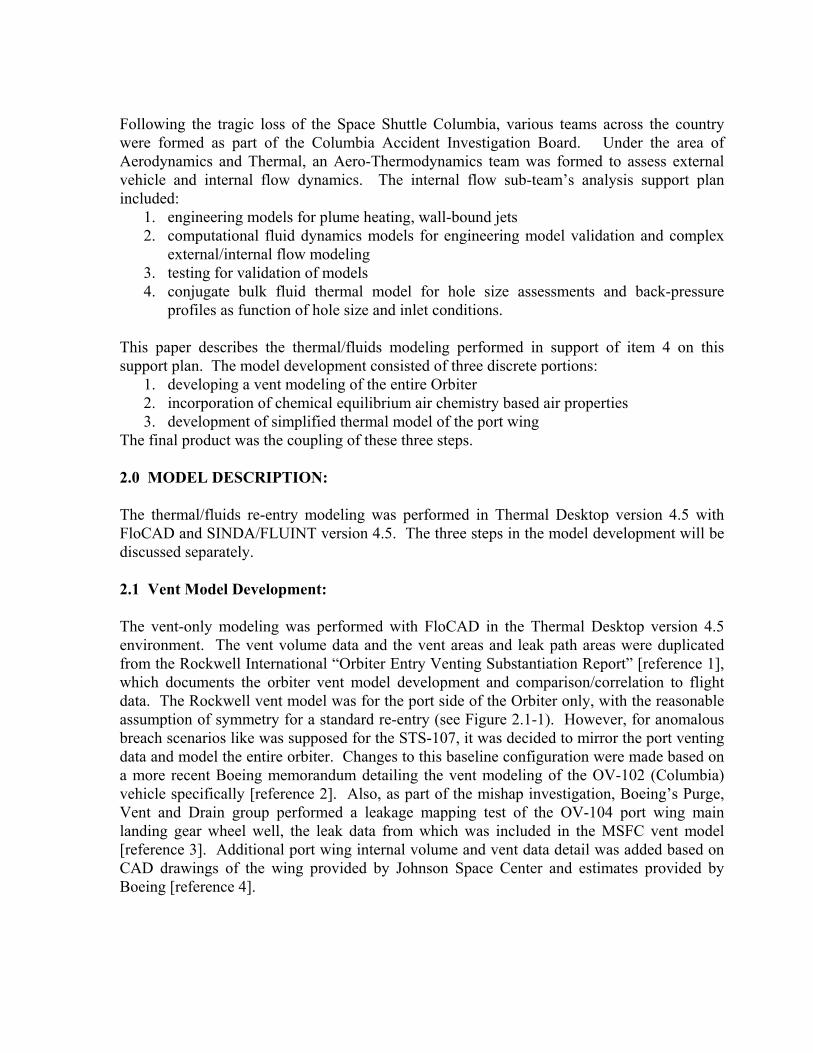
2.1.4 Breach Boundary Conditions The derivation of the local boundary conditions for a large breach is based upon the assumption that either all or a sizable fraction of the free stream total enthalpy is ingested at the breach or penetration. The flow through the large breach is modeled by the orifice device (within SINDA/FLUINT) and conditions at the upstream lump (or plenum) are updated each time-step based upon the assumed trajectory.

∞∞∞∞ γ,,, MTP

LLLL MTP γ,,,

DD TP ,FreestreamCondtions

Local Conditionsat the Breach

SINDA/FLUINTFlow Network

Representation

DD TP ,

LL TP ,UpstreamPlenum

Internal Wing Volume Lump

OrificeDevice

ConnectedWing Volumes

Figure 2.1.4-1: FLUINT Modeling of Breach Local Boundary Conditions

To determine the local conditions for the upstream boundary, the local enthalpy is scaled to the free-stream enthalpy (or taken from the engineering analysis performed by Lockheed-Martin as part of the aero-thermodynamics team) and the local pressure is derived from the free-stream pressure through an externally supplied pressure coefficient. Iteration within the equilibrium air property tables is required to determine the local conditions as a function of enthalpy and pressure for a real gas while a closed form solution exists for a perfect gas. An alternate model was created to more accurately model the period after the internal spar breach, where the local pressure from the jet impinging on the spar is assumed to equal the local

external pressure. Also, the bulk enthalpy ingested through the leading edge hole was assumed to be ingested through the spar breach (consistent with jet flow through the breach).

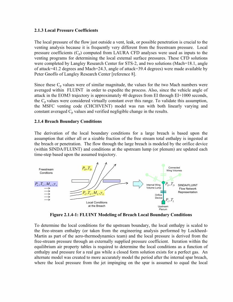
2

2∞+= ∞

uhhL

+ ∞∞= MCPP P

L2

21 γ

−

+∞=∞MTTL2

211 γ

),( LLL PhTT =Conservation of

Energy &Definition of

Pressure Coefficient

Chemical Equilibrium/Real Gas

Perfect Gas

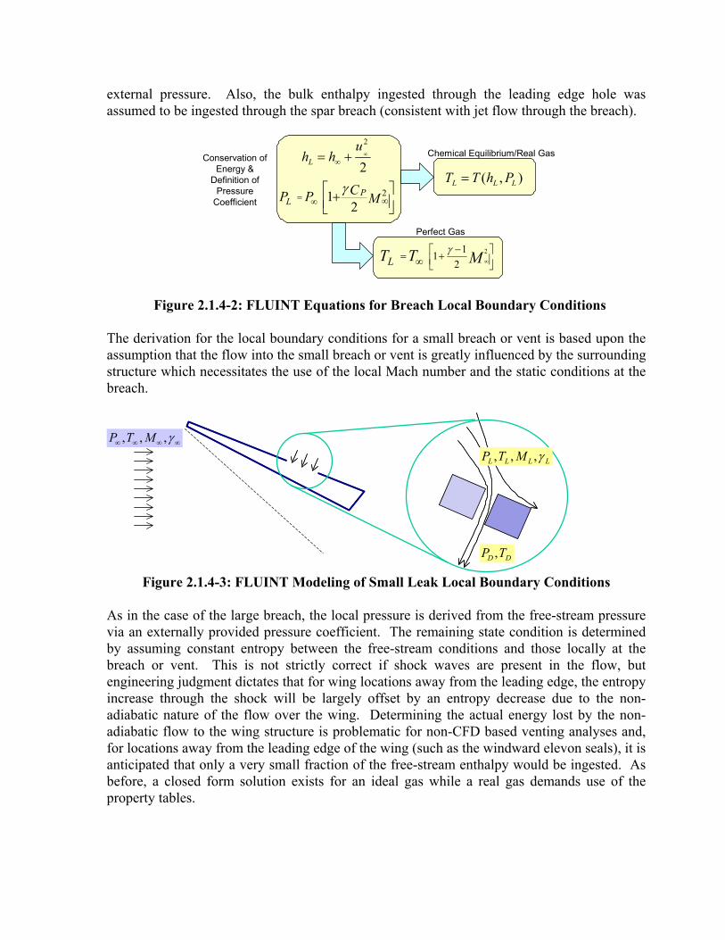
Figure 2.1.4-2: FLUINT Equations for Breach Local Boundary Conditions The derivation for the local boundary conditions for a small breach or vent is based upon the assumption that the flow into the small breach or vent is greatly influenced by the surrounding structure which necessitates the use of the local Mach number and the static conditions at the breach.

∞∞∞∞ γ,,, MTP

DD TP ,

LLLL MTP γ,,,

Figure 2.1.4-3: FLUINT Modeling of Small Leak Local Boundary Conditions

As in the case of the large breach, the local pressure is derived from the free-stream pressure via an externally provided pressure coefficient. The remaining state condition is determined by assuming constant entropy between the free-stream conditions and those locally at the breach or vent. This is not strictly correct if shock waves are present in the flow, but engineering judgment dictates that for wing locations away from the leading edge, the entropy increase through the shock will be largely offset by an entropy decrease due to the non-adiabatic nature of the flow over the wing. Determining the actual energy lost by the non-adiabatic flow to the wing structure is problematic for non-CFD based venting analyses and, for locations away from the leading edge of the wing (such as the windward elevon seals), it is anticipated that only a very small fraction of the free-stream enthalpy would be ingested. As before, a closed form solution exists for an ideal gas while a real gas demands use of the property tables.

−

−

+

−=

−

+

−

+= −

∞

∞∞

∞ 1211

12,

211

211

1

2

2

2

γγ

γ

γγ

γ

PP

MM

M

MTT

L

L

L

L

22

22∞+=+ ∞

uh

uh L

L

Chemical Equilibrium/Real Gas

Perfect Gas

∞= ssL

Conservation of Energy

Definition of Pressure Coefficient

Isentropic

( )( )LL

LL

LLLLLL

TPauhh

M

TPfhPsfT

,2

),(),(,2∞∞

∞

+−=

=⇒=ρ

+ ∞∞= MCPP P

L2

21 γ

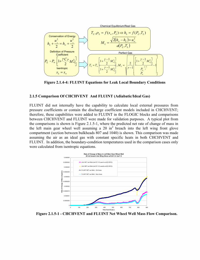
Figure 2.1.4-4: FLUINT Equations for Leak Local Boundary Conditions 2.1.5 Comparison Of CHCHVENT And FLUINT (Adiabatic/Ideal Gas) FLUINT did not internally have the capability to calculate local external pressures from pressure coefficients or contain the discharge coefficient models included in CHCHVENT; therefore, these capabilities were added to FLUINT in the FLOGIC blocks and comparisons between CHCHVENT and FLUINT were made for validation purposes. A typical plot from the comparisons is shown is Figure 2.1.5-1, where the predicted net rate of change of mass in the left main gear wheel well assuming a 20 in2 breach into the left wing front glove compartment (section between bulkheads 807 and 1040) is shown. This comparison was made assuming the air as an ideal gas with constant specific heats in both CHCHVENT and FLUINT. In addition, the boundary-condition temperatures used in the comparison cases only were calculated from isentropic equations.

Rate of Change of Mass In Left Main Gear Wheel Well

20 in2 breach into Wing Glove w/Cd=1.0, Cp=1.5

0

0.0000005

0.000001

0.0000015

0.000002

0.0000025

0.000003

0.0000035

0.000004

0.0000045

0.000005

0 100 200 300 400 500 600 700 800 900

Time from EI (sec.)

Rat

e of

Cha

nge

of M

ass

(slu

g/se

c)

chch NET ww Mdot (sts107.r10.case1a.mdt [0.0001])

chch NET ww Mdot (sts107.r10.case2a.mdt [0.0001])

FLUINT NET ww Mdot - Old Areas

FLUINT NET ww Mdot - New Areas

Figure 2.1.5-1 - CHCHVENT and FLUINT Net Wheel Well Mass Flow Comparison.

2.2 Chemical Equilibrium Air Properties

SINDA/FLUINT Property (FPROP) tables were generated using FORTRAN 90 property routines for chemical equilibrium air obtained from the NASA Langley Research Center (LaRC). Six property tables (all as a function of pressure and temperature) were generated from the property routines: specific volume, enthalpy, speed of sound, entropy, absolute viscosity, and thermal conductivity. Entropy was obtained by numerically integrating the enthalpy tables at constant pressure. SINDA/FLUINT requires entropy as a function of pressure and temperature for choking calculations in real gas simulations. Entropy tables were generated from the LaRC routines by numerically integrating the relevant Tds equation along lines of constant pressure:

[ ] 11221

212

2

1

2

1

2

1

2shh

TTTTs

constP

dPTv

Tdhds

vdPdhTds

+−+

=

=

−=

−=

∫∫∫

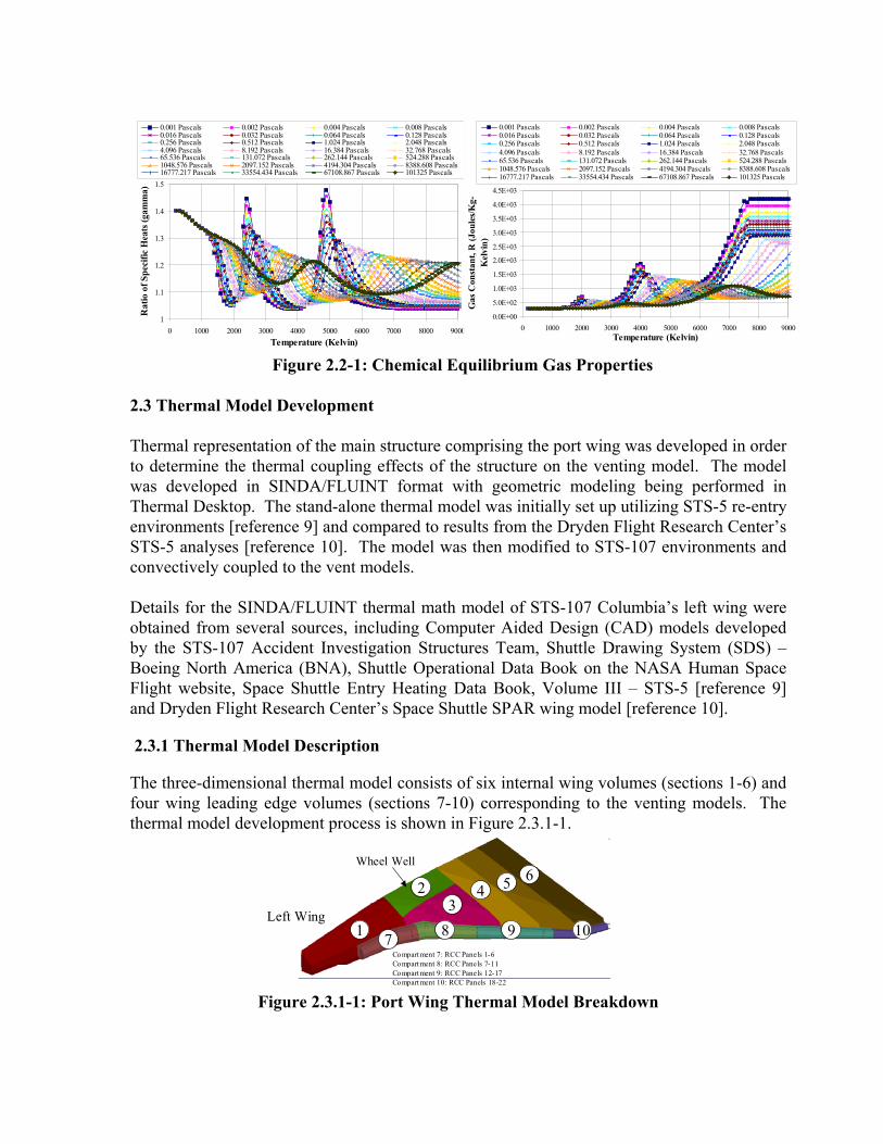
An arbitrary reference entropy of 10,000 J/kg-K (2.39 Btu/lbm-R) was chosen for the pressure equal to 0.001 Pa (9.9e-09 atms) and temperature equal to 200 K (360 R). Initial conditions for the integration were based upon ideal gas estimates of the entropy at 200 K and for a pressure range of 0.002 Pa (1.97e-08 atms) through 101325 Pa (1 atm). The trapezoidal integration was performed row-by-row with each succeeding entropy numerically integrated from the previous row’s entropy at the same pressure. The real gas properties of air are markedly different from those of a perfect gas as evidenced by the specific heat ratio and gas constant versus temperature plots shown in Figure 2.2-1. The almost cyclical changes with increasing temperature indicate a pattern of dissociation/ionization as new species are continually formed.

Also to aid choking calculations, a frozen speed of sound was computed from the specific heat ratio and an effective gas constant (REFF=P/ρT). SINDA/FLUINT utilizes internal routines to provide fluid properties either by direct interpolation or by iteration if not requested as a function of pressure and temperature (i.e. T=T[s,P]). Several of the interpolation/integration routines were rewritten to remove any dependency on ideal gas assumptions and/or to remove the additional logic present for two-phase fluids. The property tables were generated over a range of 200 K (360 R) to 9100 K (16,380 R) and from 0.001 Pa (9.9e-09 atms) to 101325 Pa (1 atm). At very low density (due to extreme temperature or low pressure), the LaRC property routines issued cautions. Some thermal conductivity and viscosity data were discarded and replaced with data obtained from the routines at a higher pressure (this is assumed reasonable given the range of pressure profiles expected in this analysis).

1

1.1

1.2

1.3

1.4

1.5

0 1000 2000 3000 4000 5000 6000 7000 8000 9000Temperature (Kelvin)

Rat

io o

f Spe

cific

Hea

ts (g

amm

a)

0.001 Pascals 0.002 Pascals 0.004 Pascals 0.008 Pascals0.016 Pascals 0.032 Pascals 0.064 Pascals 0.128 Pascals0.256 Pascals 0.512 Pascals 1.024 Pascals 2.048 Pascals4.096 Pascals 8.192 Pascals 16.384 Pascals 32.768 Pascals65.536 Pascals 131.072 Pascals 262.144 Pascals 524.288 Pascals1048.576 Pascals 2097.152 Pascals 4194.304 Pascals 8388.608 Pascals16777.217 Pascals 33554.434 Pascals 67108.867 Pascals 101325 Pascals

0.0E+00

5.0E+02

1.0E+03

1.5E+03

2.0E+03

2.5E+03

3.0E+03

3.5E+03

4.0E+03

4.5E+03

0 1000 2000 3000 4000 5000 6000 7000 8000 9000Temperature (Kelvin)

Gas

Con

stan

t, R

(Jou

les/K

g-K

elvi

n)

0.001 Pascals 0.002 Pascals 0.004 Pascals 0.008 Pascals0.016 Pascals 0.032 Pascals 0.064 Pascals 0.128 Pascals0.256 Pascals 0.512 Pascals 1.024 Pascals 2.048 Pascals4.096 Pascals 8.192 Pascals 16.384 Pascals 32.768 Pascals65.536 Pascals 131.072 Pascals 262.144 Pascals 524.288 Pascals1048.576 Pascals 2097.152 Pascals 4194.304 Pascals 8388.608 Pascals16777.217 Pascals 33554.434 Pascals 67108.867 Pascals 101325 Pascals

Figure 2.2-1: Chemical Equilibrium Gas Properties 2.3 Thermal Model Development Thermal representation of the main structure comprising the port wing was developed in order to determine the thermal coupling effects of the structure on the venting model. The model was developed in SINDA/FLUINT format with geometric modeling being performed in Thermal Desktop. The stand-alone thermal model was initially set up utilizing STS-5 re-entry environments [reference 9] and compared to results from the Dryden Flight Research Center’s STS-5 analyses [reference 10]. The model was then modified to STS-107 environments and convectively coupled to the vent models. Details for the SINDA/FLUINT thermal math model of STS-107 Columbia’s left wing were obtained from several sources, including Computer Aided Design (CAD) models developed by the STS-107 Accident Investigation Structures Team, Shuttle Drawing System (SDS) – Boeing North America (BNA), Shuttle Operational Data Book on the NASA Human Space Flight website, Space Shuttle Entry Heating Data Book, Volume III – STS-5 [reference 9] and Dryden Flight Research Center’s Space Shuttle SPAR wing model [reference 10].

2.3.1 Thermal Model Description The three-dimensional thermal model consists of six internal wing volumes (sections 1-6) and four wing leading edge volumes (sections 7-10) corresponding to the venting models. The thermal model development process is shown in Figure 2.3.1-1.

1

23

4 5 6

7 8 9 101

23

4 5 6

7 8 9 10Compartment 7: RCC Panels 1-6Compartment 8: RCC Panels 7-11Compartment 9: RCC Panels 12-17Compartment 10: RCC Panels 18-22

Left Wing

Wheel Well

Figure 2.3.1-1: Port Wing Thermal Model Breakdown

Wing internal geometry is based on the JSC-provided CAD model. The wing structural spars were included, but struts are omitted for simplicity. The main landing gear/wheel well assembly were derived from CAD model and specifications. The spar, fuselage and wheel well closeout panels are assumed to be 0.1-in thick aluminum 2219. The wing skin aluminum and aluminum-honeycomb panel representations are included. The aluminum honeycomb core is thermally modeled based on X-33 leeward aero-shell skin. The leeward honeycomb and windward honeycomb including inboard and outboard face-sheets are modeled. Thermal Protection System (TPS) is represented on both windward and leeward sides. Leeward TPS was assumed to be 0.16 inches of Flexible Re-usable Surface Insulation (FRSI) throughout (i.e., LRSI tiles were not modeled). Windward TPS assumed to be High-temperature Re-usable Surface Insulation (HRSI). Thickness was averaged for each wing section based on the Dryden model data (Reference 10). The strain isolator pad (SIP) and RTV layers in the TPS are included. Internal radiation is modeled with RadCAD (with optical properties derived from the Dryden model or estimated from the material). STS-107 wing leading edge, windward and leeward heat rates for STS-107 End of Mission (EOM) 3 trajectory were supplied by Boeing-Houston. Thermo-physical material properties were taken from (in order of preference) NASA RP-1193 or TPSX database [reference 11]. Time dependent pressure arrays (required to interpolate pressure and temperature dependent property arrays) were estimated from STS-107 EOM3 trajectory profiles, STS-2 LAURA windward and leeward Cp profiles.

2.3.2 Fluid/Structure Coupling The lumps representing the air in each of the compartment volumes in the vent models were tied convectively to the internal wing structural nodes in the thermal model. Convection coefficients for each tie were derived from laminar flow, flat plate Nusselt Number correlations [Figure 2.3.2-1, reference 12] utilizing the total flow entering each compartment, the cross-

νVL

L=Re

Am

c

CompInVρ&

≈ mCompIn&Ac

××= PrRe 3

121

664.0NuLNuL

Pr

kC pµ

=PrLNukh L= k

µ

CP = Specific Heat

= Absolute Viscosity

= Thermal Conductivity

= Prandl Number

= Nusselt Number

= Flow Area (based on comp. cross-section)

= Massflow In

where:

Figure 2.3.2-1: Heat Transfer Equations Used to Couple Venting to Thermal Modeling

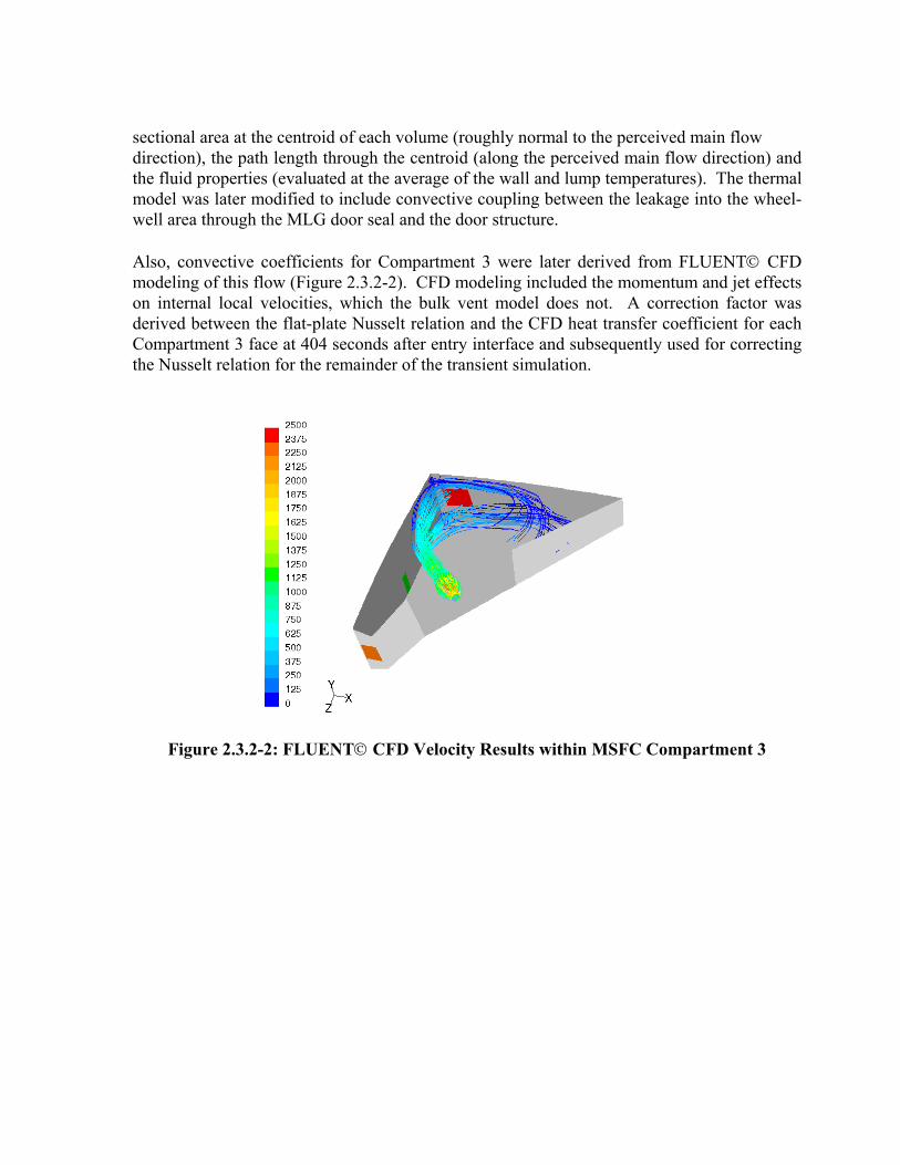
sectional area at the centroid of each volume (roughly normal to the perceived main flow direction), the path length through the centroid (along the perceived main flow direction) and the fluid properties (evaluated at the average of the wall and lump temperatures). The thermal model was later modified to include convective coupling between the leakage into the wheel-well area through the MLG door seal and the door structure. Also, convective coefficients for Compartment 3 were later derived from FLUENT CFD modeling of this flow (Figure 2.3.2-2). CFD modeling included the momentum and jet effects on internal local velocities, which the bulk vent model does not. A correction factor was derived between the flat-plate Nusselt relation and the CFD heat transfer coefficient for each Compartment 3 face at 404 seconds after entry interface and subsequently used for correcting the Nusselt relation for the remainder of the transient simulation.

Figure 2.3.2-2: FLUENT CFD Velocity Results within MSFC Compartment 3

3.0 THERMAL/VENTING RESULTS The results provided to the aero-thermodynamics team of the Columbia Investigation were generated over the course of many weeks and utilized many evolutions of the modeling. For purposes of this paper, only representative results will be given that are derived from various points in time of the modeling flow. Many of the plots provide comparisons between different cases that won’t be detailed in this paper. In addition, the reader is cautioned from attempting to draw conclusions from the data presented herein. These results don’t represent a specific scenario or set of assumptions that was determined to have caused to the Shuttle failure, but rather represents the type of parametric outputs that were provided to the team to help bracket possible causal factors.

3.1 Internal Volume Pressure Profiles The internal wing pressures are largely uninfluenced by the leading edge breach since there is only a very small nominal leak around the leading edge spar, but these pressures are dramatically increased by the subsequent internal spar breach at 487-seconds as shown in Figure 3.1-1. The bulk of the wing is freely vented, but the forward wing-glove and wheel well compartments are slightly lower due to the large venting through the Payload Bay vent in the wing-glove as illustrated by the close-up of the pressures in Figure 3.1-2.

Figure 3.1-1 – Internal Wing

Case 2

Pressure His

Case 1

tories

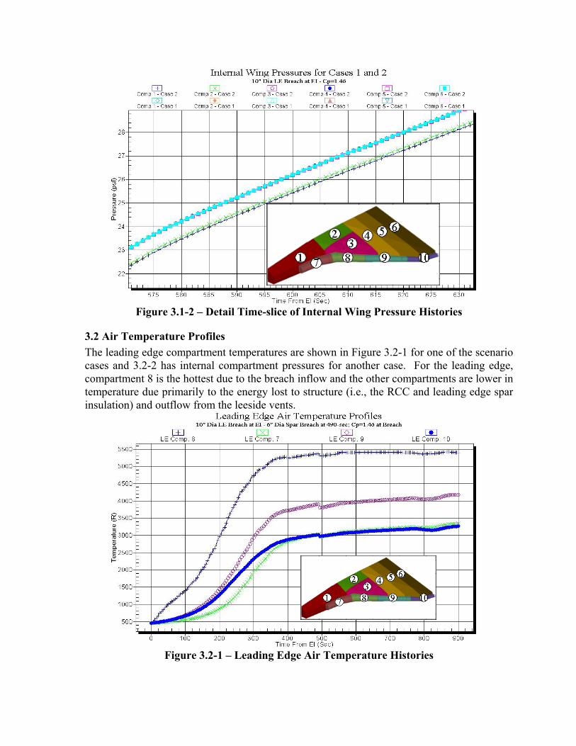
Figure 3.1-2 – Detail Time-slice of Internal Wing Pressure Histories

3.2 Air Temperature Profiles The leading edge compartment temperatures are shown in Figure 3.2-1 for one of the scenario cases and 3.2-2 has internal compartment pressures for another case. For the leading edge, compartment 8 is the hottest due to the breach inflow and the other compartments are lower in temperature due primarily to the energy lost to structure (i.e., the RCC and leading edge spar insulation) and outflow from the leeside vents.

Figure 3.2-1 – Leading Edge Air Temperature Histories

Figure 3.2-2 – Internal Wing Air Temperature Histories

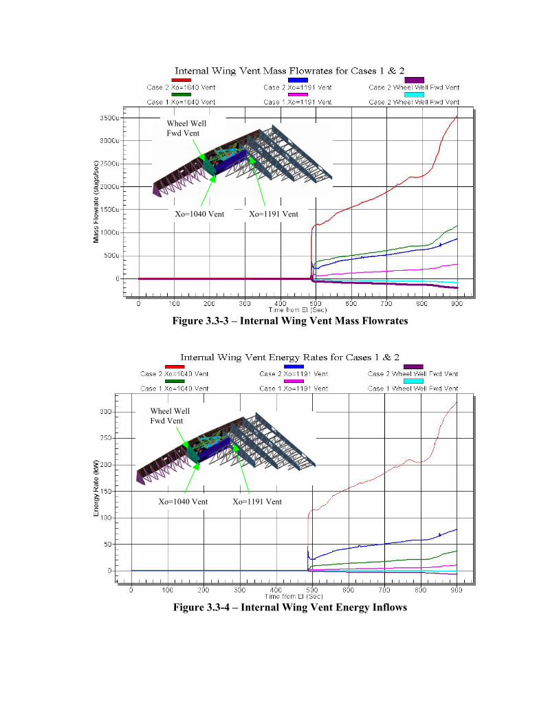
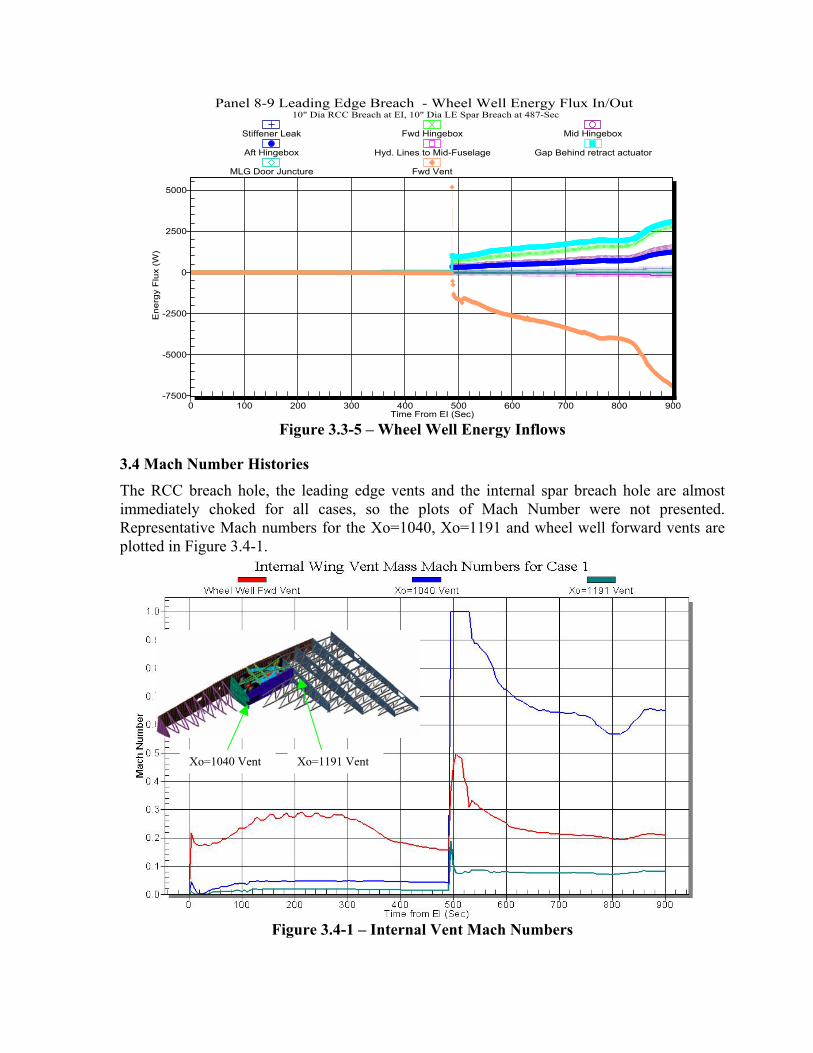
3.3 Mass Flow Rate and Energy Rate In/Out The balance between the energy flow into the RCC breach and out of the carrier panel and t-seal vents is shown in Figure 3.3-1 and the energy flux through the internal leading edge spar breach is plotted in Figure 3.3-2. The forward and aft Compartment 3 vents (at Xo=1040 and Xo=1191) and wheel well forward Xo=1040 vent mass flow rates are plotted in Figure 3.3-3. The corresponding energy rates are shown in Figure 3.3-4. The wheel well (compartment 2) was of particular interest based on the flight data. The energy rates in/out from various vents/leaks for is shown in Figure 3.3-5. This plot reveals a brief inflow through the forward vent after the breach, but then the flow begins to outflow almost immediately.

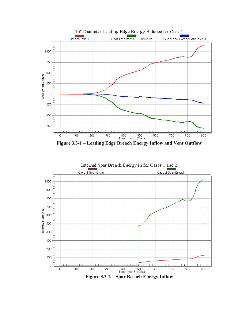
Figure 3.3-1 – Leading Edge Breach Energy Inflow and Vent Outflow

Figure 3.3-2 – Spar Breach Energy Inflow

Wheel Well Fwd Vent

Xo=1191 VentXo=1040 Vent

Figure 3.3-3 – Internal Wing Vent Mass Flowrates

Wheel Well Fwd Vent

Xo=1040 Vent Xo=1191 Vent

Figure 3.3-4 – Internal Wing Vent Energy Inflows

-7500

-5000

-2500

0

2500

5000

0 100 200 300 400 500 600 700 800 900

Panel 8-9 Leading Edge Breach - Wheel Well Energy Flux In/Out10" Dia RCC Breach at EI, 10" Dia LE Spar Breach at 487-Sec

Ene

rgy

Flu

x (W

)

Time From EI (Sec)

Stiffener Leak Fwd Hingebox Mid Hingebox

Aft Hingebox Hyd. Lines to Mid-Fuselage Gap Behind retract actuator

MLG Door Juncture Fwd Vent

Figure 3.3-5 – Wheel Well Energy Inflows

3.4 Mach Number Histories

The RCC breach hole, the leading edge vents and the internal spar breach hole are almost immediately choked for all cases, so the plots of Mach Number were not presented. Representative Mach numbers for the Xo=1040, Xo=1191 and wheel well forward vents are plotted in Figure 3.4-1.

Xo=1040 Vent Xo=1191 Vent

Figure 3.4-1 – Internal Vent Mach Numbers

3.5 Internal Wing Heat Transfer Coefficient Histories The heat transfer coefficients in Compartment 3 are shown in Figure 3.5-1. The wheel well (Compartment 2) heat transfer coefficients are plotted in Figure 3.5-2.

Figure 3.5-1 – Compartment 3 Heat Transfer Coefficients

Xo=1040

Figure 3.5-2 –

Xo=1191

Wheel Well Heat Transfer Coefficients

3.6 Solid Wall Temperature Histories The leading edge spar is insulated with Cerachrome that has a thin outer layer of Inconel. The Inconel temperature is plotted in Figure 3.6-1. Local heating effects caused by the leading-edge breach jet impinging on the insulation are not modeled and therefore the resultant temperatures for Compartment 8 are lower than what would be expected. However, for compartments away from the breach (7, 9, and 10) the predicted Inconel temperatures are considered conservative and indicate that the insulation would remain intact. The Compartment 3 wall skin temperatures are shown in Figure 3.6-2. Note that the temperatures for the case presented exceed the aluminum melting point for many of the areas, which is known not to be the case from the telemetry data. This indicates that this particular case included too much energy flowing into the wing (as compared to actual) due to either too large a size of the breach holes or the ingested enthalpy with local pressure assumptions being too high. 3.7 Structural Pressure Differential Across Leading Edge One special case that was requested involved plotting the pressure differential across the leading edge spar for 6” and 10” RCC breaches without an internal spar breach (Figure 3.7-1). This was to be used by structural engineers in assessing potential structural failures.

~Inconel Melt Temperature

NOTE: Doesn't includejet impingement heatingonto Cerachrome - onlyflow-based convectiveheat transfer

Figure 3.6-1 – Leading Edge Cerachrome Insulation Inconel Outer Layer Temperature

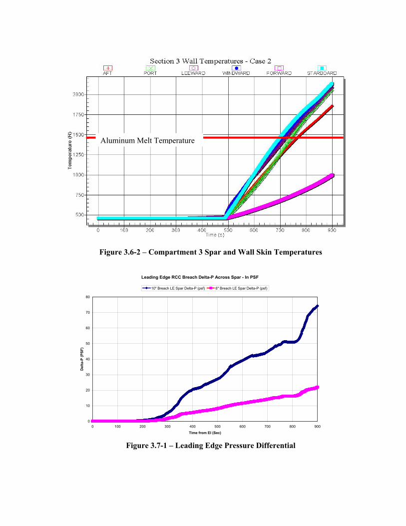
Aluminum Melt Temperature

Figure 3.6-2 – Compartment 3 Spar and Wall Skin Temperatures

Leading Edge RCC Breach Delta-P Across Spar - In PSF

0

10

20

30

40

50

60

70

80

0 100 200 300 400 500 600 700 800 900

Time from EI (Sec)

Del

ta-P

(PSF

)

10" Breach LE Spar Delta-P (psf) 6" Breach LE Spar Delta-P (psf)

Figure 3.7-1 – Leading Edge Pressure Differential

ACKNOWLEDGEMENTS The authors would like to acknowledge the assistance of Leslie Gong and William Ko of NASA Dryden Flight Research Center in providing the thermal models that were generated of the port wing for re-entry heating comparison to the STS-5 flight. These models were a very valuable source of information in creating a simplified model of the wing for this coupled venting/thermal effort. Also, Mr. William Downs and Stuart Nelson of NASA Marshall Space Flight Center are acknowledged for the generation of the CHCHVENT venting model that was utilized in correlating the FLUINT venting model. Also, we want to acknowledge Mr. Maurice Prendergast of NASA Marshall Space Flight Center who assisted in the creation of the SINDA thermal math model of the port wing as well as the documentation of the thermal modeling assumptions. ACRONYMS: BNA Boeing North America CAIB Columbia Accident Investigation Board CAD Computer Aided Design CFD Computational Fluid Dynamics CHCHVENT CHamber-to-Chamber Vent (Program) EI Entry Interface EOM3 End of Mission 3 FRSI Flexible Re-usable Surface Insulation HRSI High-temperature Re-usable Surface Insulation JSC Johnson Space Center LaRC Langley Research Center LAURA LaRC’s finite volume fluid flow CFD solver MLG Main Landing Gear MSFC Marshall Space Flight Center NASA National Aeronautics and Space Administration OV Orbiter Vehicle RCC Reinforced Carbon-Carbon SDS Shuttle Drawing System SIP Strain Isolation Pad STS Space Transportation System TPS Thermal Protection System β Beta Angle γ Ratio of Specific Heats ρ Density Cd Discharge Coefficient h Enthalpy M Mach Number P Pressure R Universal Gas Constant s Entropy T Temperature

REFERENCES:

1. Wong, Lung-Chuen, et al, “Orbiter Entry Venting Substantiation Report.” Rockwell International Space Systems Division, SSD94D0275, September 1994.

2. Cline, D.E., “As Built OV-102, Flight 27, STS-109 Integrated Vent Model,” Boeing Company-Houston, DWC-2002-003, April 10, 2002.

3. Cline, D.E. and Torres, “Main Gear Wheel Well Leakage Mapping and Model,” presentation to Aero-Thermal Mishap Investigation team, Boeing-PVD, March 2003.

4. Electronic mail from Lung-Chuen Wong/Boeing entitled “Wing Leading Edge Vent Areas”, 4/16/03.

5. Fay, J.F. “Program CHCHVENT Version 5 User’s Manual and Software Description.” Sverdrup Technology/MSFC Group, Report 631-001-93-007, November 1993.

6. Shapiro, Ascher H. The Dynamics and Thermodynamics of Compressible Fluid Flow, Volume 1, New York: John Wiley & Sons, 1953.

7. Haukohl, J., and Forkois, J.L. “Inflow Venting Orifice Efficiency Test Report.” Lockheed Missiles & Space Company Report LMSC-HREC D225598, January, 1972.

8. Gnoffo, P.A., Weilmuenster, K.J., and Alter, S.J., “A Multiblock Analysis for Shuttle Orbiter Re-entry Heating from Mach 24 to Mach 12,” NASA CP 3248, April 1995.

9. Hartung, Lin C., Throckmorton, David A., “Space Shuttle Entry Heating Data Book, Volume III – STS-5”, NASA RP-1193, May 1988.

10. Gong, Leslie, Ko, William L., Quinn, Robert D., “Thermal Response of Space Shuttle Wing During Reentry Heating”, NASA TM-85907, June 1984.

11. Thermal Protection Systems Expert and Material Property Database (TPSX), Web Edition Version 3, NASA Ames Research Center, 2003.

12. Incropera, Frank P., Dewitt, David P., “Fundamentals of Heat and Mass Transfer”, Second Edition, John Wiley and Sons, Inc., 1985.