Intermittency and the cost of integrating solar in the … and the cost of integrating solar in the...

Intermittency and the cost of integrating

solar in the GB power market

September 2016

AURORA ENERGY RESEARCH 2

Foreword

This report commissioned by the Solar Trade Association was prepared by Aurora

Energy Research.

The analysis represents Aurora’s independent views. The assumptions made and

forecasts underpinning the analysis are consistent with Aurora’s widely used GB

Power Market Quarterly Forecast, unless noted otherwise.

For more information about Aurora Energy Research, see www.auroraer.com.

About Aurora Energy Research

Aurora Energy Research is an independent energy market analytics firm, providing

data, forecasts and insights on UK, European and global energy markets. Our power

market models simulate wholesale, balancing and capacity markets, and economic

investment decisions across all generation technologies (including battery storage)

to provide internally consistent forecasts. Our reports and advisory work provide

unique and powerful insights to our clients and subscribers who include generators,

developers, banks, regulators and NGOs.

http://www.auroraer.com/


Contents

Executive Summary ................................................................................................... 4

1. Introduction .......................................................................................................... 6

1.1. Context .......................................................................................................... 6

1.2. Defining intermittency cost ............................................................................ 6

1.3. Other costs and benefits associated with renewable power .......................... 9

2. The cost of intermittency for solar PV today ...................................................... 10

3. The cost of intermittency for solar PV in the future ............................................ 12

3.1. 40GW of solar by 2030 ............................................................................... 12

3.2. Lesser levels of solar penetration by 2030 .................................................. 13

4. The impact of other generation technologies on solar intermittency costs ......... 15

4.1. The impact of additional wind ...................................................................... 15

4.2. The impact of no new nuclear ..................................................................... 16

4.3. The impact of large-scale battery penetration ............................................. 18

5. Conclusion ......................................................................................................... 21

Technical appendix .................................................................................................. 22

Aurora’s power market modelling approach .......................................................... 22

Key assumptions ................................................................................................... 22


Executive Summary

As renewable power capacity increases in Great Britain’s electricity system,

assurance is needed that the costs of integrating and managing the intermittency

associated with renewable power, such as solar, is manageable. Greater articulation

of the system costs will also enable fairer competition with other sources of low-

carbon power and more informed policy choices.

In this report we estimate the current and future costs of intermittency for solar, that

is, the cost of integrating and backing up solar’s variable output, rather than the cost

of generating the solar power in the first place.

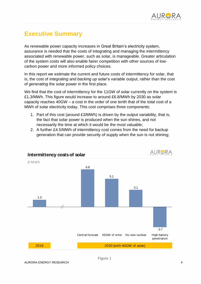
We find that the cost of intermittency for the 11GW of solar currently on the system is

£1.3/MWh. This figure would increase to around £6.8/MWh by 2030 as solar

capacity reaches 40GW – a cost in the order of one tenth that of the total cost of a

MWh of solar electricity today. This cost comprises three components:

1. Part of this cost (around £3/MWh) is driven by the output variability, that is,

the fact that solar power is produced when the sun shines, and not

necessarily the time at which it would be the most valuable;

2. A further £4.5/MWh of intermittency cost comes from the need for backup

generation that can provide security of supply when the sun is not shining;

AE

R T

em

pla

te 2

01

6a

Intermittency costs of solar

-3.7

3.1

5.1

6.8

1.3

No new nuclearCentral forecast 45GW of wind High battery

penetration

£/ MWh

2030 (with 40GW of solar)2016

Figure 1


and

3. Balancing costs passed onto the system by solar are more than offset by the

additional system flexibility provided by the backup generation brought on.

The presence of substantial backup capacity has the side benefit of reducing

the costs of balancing, taking £0.7/MWh off the overall intermittency cost.

With additional wind on the system (up to 45GW by 2030), we find that the cost of

intermittency for solar would be reduced to £5.1/MWh. This demonstrates the benefit

of a diverse renewables portfolio, as solar and wind deliver their output at different

times.

We further find that such an intermittency cost would be reduced in a scenario with

no further nuclear build out to around £3.1/MWh, due to the more flexible alternative

generation technologies we would expect to see emerge from the capacity market in

the absence of new nuclear.

A scenario with cheaper batteries would also have a lower solar intermittency cost.

Batteries allow excess power to be delivered at a more valuable time and reduce the

need for backup generation. In a scenario with 8GW of batteries on the system by

2030, we find the overall intermittency cost would in fact become negative, falling to

around £-3.7/MWh. This effectively means that the intermittency of solar provides a

net benefit through enabling the entry of batteries.

In the context of rapidly falling solar and wind generation costs and an increasing

need for affordable low-carbon power, we do not see these costs as a major barrier

to further renewable penetration.


1. Introduction

1.1. Context

As the amount of renewable generation on the system increases, the challenges and

costs associated with integrating the intermittent output into the energy system are

more commonly being considered in the debate about renewables subsidies and

build-out rates.

The “cost of intermittency” is a many-facetted concept, requiring detailed analysis to

quantify. The most common and intuitive claim against renewable generation is that

it cannot deliver if the wind does not blow and the sun does not shine, and therefore

results in either an unreliable generation system or one with a large amount of costly

backup capacity.

While this report focuses on the cost of integrating renewables, it also acknowledges

that renewable generation has significant benefits. For instance, renewables provide

power that is carbon-emission free. Furthermore, the costs of many renewable

technologies are falling rapidly and are may be cheaper on a per MWh1 basis than

fossil fuel alternatives in the future.

Understanding the costs of variable renewable generation is important in order to

identify the most cost-effective pathways for decarbonising the power system, and

for enabling the true comparison of generation options, or fair competition between

technologies, within the available carbon budgets.

It is this intermittency cost that we seek to both define and quantify in this report with

a view to informing the broader debate about the best generation mix for the GB

economy. The quantification and forecasting of intermittency costs is highly

technical, and underpinned by Aurora’s system-level energy market model that

forecasts simultaneously across energy, capacity and balancing markets. As much

as is possible, this report focusses on the results and implications of the modelling

and analysis rather than on detailed and technical discussions of methodology.

1.2. Defining intermittency cost

We define the cost of intermittency as:

1 Megawatt-hour, an amount of electricity worth around £50 in the wholesale market.


The external2 costs imposed on the energy system resulting from the

timing and predictability of a given generation technology’s power output

relative to a case where the same number of MWhs are generated evenly

over every hour of the year.

By focusing on net external costs, we exclude costs of intermittency that are

paid for by the renewable asset owner and count only those costs borne by

other market participants or the consumer. By comparing the renewable

technology’s output to an alternative scenario where the only changed factor is

the timing of the output, we are able to focus exclusively on intermittency costs.

This is distinct from comparisons that also include other cost differences such

as construction and operating costs.

The term “intermittent” is commonly used to describe the output from solar and

wind, but some industry analysts prefer the term “variable” to describe such

generation. For example, the International Energy Agency (IEA) refers to solar

and wind generation as variable renewable electricity. For the purposes of this

report, we use intermittent and variable synonymously to describe the output of

solar.

We break down the total intermittency cost into three component parts, each of

which can be quantified separately and easily understood.

1.2.1. Timeliness of delivery

“Not all MWhs are created equal”.

A MWh delivered at times of the year when demand is high and supply is low is

inherently more valuable than a MWh delivered when demand is low and supply is

high.

This constantly changing value of a MWh of electricity is efficiently represented by

the wholesale power price, something that can be readily observed and forecasted

with half-hourly resolution. The wholesale power price can vary dramatically over the

course of a year to over £100 per MWh in high demand/low supply periods and to

negligibly low or even negative levels when demand is low and supply is high.

So to quantify the extent to which the timeliness of delivery adds or subtracts value

from the MWh of electricity produced by driving out more expensive forms of

generation and reducing the wholesale power price, we calculate the weighted

average wholesale power market price in all the hours of a year when power is

2 That is, the costs passed on to the energy system and ultimately paid by the consumer rather than paid for by

the generation asset itself


typically delivered by a given technology (sometimes called the “capture price”) and

compare it to the baseload power price. If the capture price is on average less than

the baseload power price, then the timeliness of delivery of the MWhs produced over

a year is disadvantaging this generation technology against a baseload alternative.

1.2.2. Need for backup generation

“When the wind doesn’t blow and the sun doesn’t shine”.

The second component of intermittency cost we describe is the need for backup, that

is, in the event that the wind does not blow and the sun does not shine, there is a

cost of maintaining sufficient backup generation on the system to keep the lights on

year around. This backup generation is typically gas- or diesel-fired generation, and

in the future will also be provided by batteries.

Whilst intuitively a simple concept, quantifying it is difficult. The calculation has to be

done at a system level, and with consideration of the “averaging effect” that a diverse

set of technologies, geographic locations and weather patterns can offer. This

averaging effect means that the backup cost at a system level is less than the cost of

backing up every individual renewable asset with a dedicated gas or diesel plant that

does nothing other than even out the generation output or guarantee delivery during

times of system stress.

The backup cost must also take into consideration the revenue such backup capacity

can capture by simultaneously offering other services to the market in addition to the

backup of renewables. If, for example, a backup plant could provide an ancillary

service such as frequency response without this interfering with its ability to provide

backup, the net cost to the system of the backup capacity would be less.

We calculate this cost at a system level by calculating the amount and type of

generation that would enter the power system via the capacity market in order to

provide the necessary security of supply3 for a given level of renewable penetration,

and compare this to the case where renewable generation output is evenly

distributed and hence less backup capacity enters the system.

1.2.3. Short-term forecasting accuracy

“Does it deliver exactly when it says it will?”

The third and final component of the cost of intermittency we describe as “short term

forecasting accuracy”, that is, the degree to which the technology delivers the power

3 Technically, this is determined by the 3-hour Loss of Load Expectation (LOLE) specified in the capacity market

design


it says it will, 30 minutes ahead of time. This time window is important since it

corresponds to the operation of the balancing market, where supply and demand are

balanced in real time by the system operator.

Wind and solar, like all generators, will submit their expected output to the system

operator 30 minutes in advance of delivering it. If the weather then changes and the

power cannot be delivered, the system operator will procure other sources of

generation at short notice and the renewable generator will be penalised for non-

delivery.

While the financial penalty for non-delivery of the renewable power known as the

“cash-out price” is borne by the asset owner and therefore not included in our

definition of intermittency cost, there is a subtler knock-on effect to the cash-out price

itself, with more demand for balancing driving up the cash-out price paid by the rest

of the system. It is these additional costs we quantify as the impact of short-term

forecasting accuracy.

1.3. Other costs and benefits associated with renewable power

We do not quantify the impact renewables have on transmission and distribution

costs or benefits in this report. Any such costs paid for by the renewable developer

or asset owner would in any case not be included, but there are other costs

renewables can impose on transmission and distribution by exacerbating congestion

and increasing the amount of capacity required to cope with low utilisation and

volatile demand. Conversely distributed renewables can defer or avoid more

expensive grid reinforcement costs at higher voltages.

We do however capture the impact on headroom and footroom, and balancing

mechanism constraint management through our balancing market modelling.

We do take account of what are sometimes called spill costs, where not all power

from renewable generation can be used and is ‘spilt’, typically by paying the

generator not to deliver it. This is accounted for in our ‘timeliness of delivery’

category, since power produced and not used is by definition worthless and thus

drags down the capture price.

Our ‘timeliness of delivery’ measure also takes into account the merit order effects

of power system. This effect occurs when solar is generating, which reduces the

generation required from other technologies and thus changes the power price and

the total cost of the power system.


2. The cost of intermittency for solar PV today

We currently have around 11 GW of solar generation on the GB power system,

which includes all types of solar from domestic rooftops to ground mounted solar

farms. At these levels, we estimate solar’s cost of intermittency today is around

£1.3/MWh.

Figure 2

For solar, we see the timeliness of delivery explaining about £-1.2/MWh of the cost

since solar delivers its output at times when the power price is higher than the

baseload price. Solar has the advantage of delivering output during the day when

demand is higher rather than overnight when demand is lower. However as solar

penetration levels increase over time, so much power may be available during sunny

AE

R T

em

pla

te 2

01

6a

Intermittency costs of solar in 2016

-1.2

1.3

Timeliness

of delivery

Need for backup TotalForecasting

accuracy

2.5

0.0

£/ MWh


periods that the wholesale price is pushed own and solar cannibalises its own

capture price.

The need for backup capacity for solar creates a corresponding intermittency cost of

£2.5/MWh. As the capacity market is not yet enacted in 2016, we use instead the

cost of reserve capacity4 to quantify the cost of backup for the existing renewable

generation.

The cost associated with short-term forecasting accuracy we find to be roughly zero

today. This is not because there is no forecasting error; unexpected under- or over-

delivery does occur and the cost associated with this is borne by the generator (and

thus not included in the cost of intermittency). Rather, current levels of solar

penetration have a negligible impact on the overall cost of balancing the system

because its forecasting errors diffused at a system level by wind and demand

uncertainty.

4 National Grid has procured 3.5GW of Supplemental Balancing Reserve (SBR) for the winter of 2016/17, used to

ensure security of supply.


3. The cost of intermittency for solar PV in the future

3.1. 40GW of solar by 2030

To understand the impact a future increase in solar penetration may have on

intermittency cost, we have simulated the evolution of the energy market under a

scenario where the total installed solar capacity increases from 11GW today to

40GW by 2030.

With this increased solar penetration, capture price cannibalisation begins to occur.

This increases the intermittency cost associated with the timeliness of delivery from

£-1.2/MWh today to £3/MWh by 2030. While solar continues to benefit from

delivering much of its power during peak summer afternoon periods, eventually so

much power is delivered at these times that thermal generation with a higher

marginal cost is frequently not required, and the capture price falls.

The cost of backup capacity for solar increases from £2.5/MWh today to £4.5/MWh

by 2030. The high penetration of solar on the system necessitates more backup

procured through the capacity market. The backup procured would also require

higher capacity payments to incentivise entry as the high levels of solar lowers day

time power prices.

Because of this increased backup capacity, the impact of the short-term

‘forecastability’ of solar is £-0.7/MWh, which is a net benefit. The reason for this is

that the substantial backup capacity that emerges to ensure security of supply is

flexible generation. This capacity plays into the balancing mechanism, and a useful

side effect is to reduce the cash-out price and therefore balancing cost paid by the

rest of the generation fleet.


Figure 3

3.2. Lesser levels of solar penetration by 2030

With lower levels of solar penetration, the intermittency cost of solar is also lower.

From model simulations with incremental levels of solar penetration (with 2030 solar

capacity at 12GW, 15GW, 20GW etc.), we find that there is a near linear relationship

between solar capacity and its intermittency cost, not the ‘exponential’ increase that

might be expected at these penetration levels. A doubling of solar capacity from

today’s 11GW would bring the cost of intermittency from £1.3/MWh to £3.4/MWh.

Additional solar capacity primarily increases the intermittency cost associated with

timeliness of delivery. High solar penetrations push down the power price when solar

delivers its output and thus cannibalises the capture price.

Higher levels of solar capacity also increase the costs for the need for backup. The

added solar cannot be used to meet the winter peaks, so there is an additional cost

to procure adequate backup generation to ensure security of supply.

AE

R T

em

pla

te 2

01

6a

Intermittency costs of solar by 2030, with 40GW of solar

4.5

3.0

6.8

Need for backup TotalForecasting

accuracy

-0.7

Timeliness

of delivery

£/ MWh, average 2025-2035


Figure 4

AE

R T

em

pla

te 2

01

6a

Intermittency cost of solar by 2030, at different levels of solar penetration

0

1

2

3

4

5

6

7

8

10 15 20 25 30 35 40


2016

capacity

Solar capacity (GW)


4. The impact of other generation technologies on

solar intermittency costs

4.1. The impact of additional wind

Solar output is delivered at different times than wind output, and thus having both on

the system allows for their intermittency to be diversified. In a system with a lot of

wind, the ability of solar to generate at times when there is less wind output becomes

proportionately more valuable.

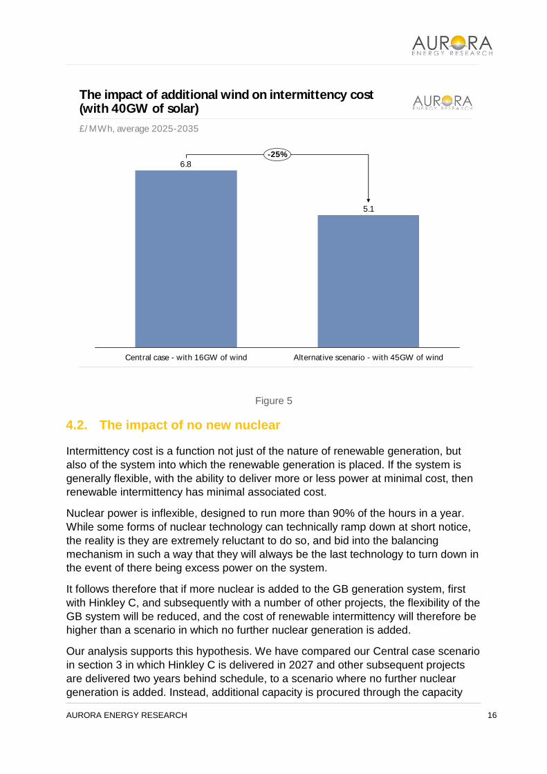
We quantify this portfolio benefit by comparing our central case, in which we hold

today’s 16GW of wind constant, to a scenario with wind capacity reaching 45GW by

2030.

As the additional wind contributes a small amount to the security of supply in winter

months, there would be a slight reduction in generation procured through the

capacity market in this scenario. We find that the additional 29GW of wind capacity

decreases the intermittency cost of solar from £6.8/MWh to £5.1/MWh, a difference

of about one quarter.

The main added value of solar when there is additional wind is through the improved

timeliness of delivery. The high wind penetration would depress prices whenever

wind generates, which is often overnight and in the winter. However, solar output is

generated in the daytime and at higher volumes during the summer. This allows

solar to avoid the lower prices caused by wind generation and achieve an improved

capture price relative to the baseload price.

While wind also creates an own intermittency cost of its own, the ability of additional

wind to reduce the intermittency cost of solar (and vice versa) highlights the value of

having a diversified portfolio of renewables on the system.


Figure 5

4.2. The impact of no new nuclear

Intermittency cost is a function not just of the nature of renewable generation, but

also of the system into which the renewable generation is placed. If the system is

generally flexible, with the ability to deliver more or less power at minimal cost, then

renewable intermittency has minimal associated cost.

Nuclear power is inflexible, designed to run more than 90% of the hours in a year.

While some forms of nuclear technology can technically ramp down at short notice,

the reality is they are extremely reluctant to do so, and bid into the balancing

mechanism in such a way that they will always be the last technology to turn down in

the event of there being excess power on the system.

It follows therefore that if more nuclear is added to the GB generation system, first

with Hinkley C, and subsequently with a number of other projects, the flexibility of the

GB system will be reduced, and the cost of renewable intermittency will therefore be

higher than a scenario in which no further nuclear generation is added.

Our analysis supports this hypothesis. We have compared our Central case scenario

in section 3 in which Hinkley C is delivered in 2027 and other subsequent projects

are delivered two years behind schedule, to a scenario where no further nuclear

generation is added. Instead, additional capacity is procured through the capacity

AE

R T

em

pla

te 2

01

6a

The impact of additional wind on intermittency cost (with 40GW of solar)


5.1

6.8

-25%

Central case - with 16GW of wind Alternative scenario - with 45GW of wind


market. By modelling the competition of technologies in the capacity market

auctions, we find that a combination of CCGT, demand side response, battery

storage and reciprocating engines will take the place of nuclear.5

We find that replacing new nuclear generation with more of these more flexible forms

of generation decreases the intermittency cost of solar from £6.8/MWh to £3.1/MWh,

more than halving the cost.

This benefit is driven by two forces, each in roughly equal proportion. First, related to

the timeliness of delivery: the absence of ‘must run’ nuclear means that high

renewable penetration causes less cannibalisation of its own capture price. When

renewable output is high, flexible generation simply shuts down and prices remain

relatively high compared to our Central case scenario where new nuclear stays

running and prices fall by a greater amount.

Second, the cost of backup also falls in the no new nuclear scenario. With no new

nuclear, existing CCGT runs higher load factors and incurs less ramping cost to

deliver the flexibility demanded by additional solar. As a result, it is more profitable

and bids less in the capacity market, driving down the capacity market clearing price

and the cost of backup.

5 Such a scenario would also increase carbon emissions. There are alternative generation mixes with a lower

carbon impact that could also replace new nuclear, including additional renewable generation.


Figure 6

It should be noted that this alternative scenario with no nuclear, whilst benefiting

from the additional flexibility of CCGT and other technologies, is expected to also

have higher carbon emissions. An alternative scenario with comparable carbon

emissions would inevitably require more renewables, and hence the intermittency

cost may be higher rather than lower. Further, while the existence of new nuclear

drives the cost of intermittency up, the magnitude is relatively small and unlikely to

shift the overall cost-benefit economics of new nuclear.

4.3. The impact of large-scale battery penetration

The prospects for grid-scale energy storage have recently become significantly more

promising. This has been driven primarily by substantial decreases in the cost of

lithium ion batteries, to the point where the investment case for batteries for a wide

range of applications is likely to be viable in the next five years. For niche

AE

R T

em

pla

te 2

01

6a

The impact of no new nuclear on intermittency cost (with 40GW of solar)


3.1

6.8

Central case - with new nuclear

-55%

Alternative scenario - no new nuclear


applications such as frequency response, battery technology is already being rolled

out in the GB market6.

Aurora estimates that if costs continue to decrease to the level of £100/kWh by the

early 2020s (today the cost is nearer £300/kWh), economically attractive investment

opportunities for up to 8GW of batteries would arise on the GB electricity system by

2030.

In our central case scenario in section 3 we assumed only modest cost

improvements in batteries of 4 percent per annum, and thus negligible battery

penetration, but here we consider the impact that 8GW of batteries could have.

Batteries are a natural counterpart to renewable generation, allowing excess power

to be stored and released back onto the system when it is needed, thus reducing the

cost of intermittency.

We estimate solar’s cost of intermittency falls from £6.8/MWh without batteries to £-

3.7/MWh with batteries i.e. there is a system benefit rather than a cost. This is due to

two factors: firstly, the existence of batteries on the system smooths out prices in the

energy and balancing markets, thus reducing the impact that the timeliness of

delivery has on intermittency cost. Second, batteries play a useful role in the

capacity market, reducing capacity prices and therefore the cost of backup for

renewables.

With a large amount of batteries on the system, solar has a ‘negative cost’ of

intermittency, meaning that the generation profile of solar is actually more desirable

for a battery-enabled system than a baseload-equivalent output profile. Batteries and

solar are a complementary combination, with batteries improving the capture prices

of solar, and solar creating a generation profile whereby batteries can profitably store

and then deliver to the market as needed.

6 200 MW of primarily battery storage generation was procured by National Grid for ‘enhanced frequency

response’ in August 2016.


Figure 7

AE

R T

em

pla

te 2

01

6a

The impact of high battery penetration on intermittency cost (with 40GW of solar)


-3.7

6.8

Central case - minimal battery penetration Alternative scenario - high battery penetration

-155%


5. Conclusion

Returning to the question posed at the start of this report, do intermittency costs

present a major hurdle to the further penetration of renewable generation?

Our analysis has shown that substantial further solar penetration is possible and

affordable. Security of supply can be maintained, with sufficient flexible capacity

emerging to manage the intermittency associated with up to 40GW of solar at a

modest cost.

With intermittency costs today of around £1.3/MWh for solar, increasing to £6.8/MWh

with a substantial 40GW of solar on the system by 2030, we would suggest these

costs do not provide a strong argument against the further build out of renewable

generation.

While £6.8/MWh of additional cost on top of the cost of each MWh of renewable

power generation is a non-trivial amount, when set against the substantial year-on-

year cost decreases being exhibited by both wind and solar and the benefits of a

renewable low carbon power source, these costs are justifiable and competitive with

fossil fuel alternatives.

Furthermore, the figure of £6.8/MWh of intermittency cost by 2030 represents a

‘worst case’ scenario; Should battery costs fall to £100/kWh as many commentators

expect they will, if wind power grows significantly, or if new nuclear is cancelled or

delayed, intermittency costs will be lower or could in fact be negative.


Technical appendix

Aurora’s power market modelling approach

The analysis for this report is underpinned by the Aurora Energy Research Electricity

System model for Great Britain (“AER-ES GB”). This model, which was

independently developed by Aurora Energy Research, is a market-leading dynamic

dispatch model used by many major private and public sector participants in the GB

and European power markets to forecast plant performance and valuation.

Given a set of assumptions around solar buildout, policy, fuel prices and

technological progress, Aurora’s model calculates the economic entry and exit of

other generation types through the capacity market based on economic incentives.

In the context of this report the model has been used to estimates the capacity mix

that would result from different levels of solar penetration based on half-hourly

electricity and system prices and yearly capacity prices.

Key assumptions

The assumptions that underpin the analysis presented in this report are consistent

with Aurora’s quarterly GB Power Market Forecast (2016 Q3).

GB carbon price trajectory

In our modelling, we assume that the Carbon Price Support (“CPS”) freeze will last

until 2019/20, as currently legislated. Beyond 2020 we assume that the CPS will be

adjusted year-by-year so as to achieve the government’s target carbon price

trajectory (Carbon Price Floor – “CPF”), taking into account the evolution of the

European price of carbon – the EU Emissions Trading System (“EU ETS”) allowance

(“EUA”). During this period, we assume the carbon price trajectory will rise from the

level of £22/tonne in 2020 to £40/tonne in 20407.

Figure 8 summarises our carbon price assumptions. With weak EUA prices, and the

UK’s ambition to lead the EU’s decarbonisation effort, we forecast a policy-driven GB

carbon price that is above the price of European emission allowances. However, we

also disaggregate our overall carbon price into EUA and CPS outlooks and report

our official EUA forecast separately (see below).

7 We do not specify the measure of these values contributed by the CPS, as we assume that it is adjusted

accordingly in order to adhere to these targets. Our implicit assumption is that the EUAs prices do not exceed this trajectory.


Figure 8

EU ETS allowance price trajectory

In our modelling of the EUA prices, we account for recent policy developments,

including 2030 targets for decarbonisation, renewables deployment and efficiency

improvements, as well as the tightening of emission caps under Phase IV of the

ETS, and the introduction of the Market Stability Reserve.

To produce our internal EUA forecast, we employ a hybrid modelling approach that

links our European power dispatch model AER-ES EU and our global general

equilibrium model AER-GLO. The hybrid model solves for the price of carbon

required to achieve a given carbon emissions cap in each year. The combination of a

general equilibrium model that captures all economic activity, and a power dispatch

model, captures the detailed mechanics of fuel substitution in the power sector at an

AE

R T

em

pla

te 2

01

6a

Aurora carbon price

0

5

10

15

20

25

30

35

40

45

50

20

33

20

29

20

27

20

21

20

40

20

38

20

36

20

39

20

35

20

34

20

37

20

32

20

31

20

30

20

28

20

26

20

25

20

24

20

23

20

22

20

20

20

19

20

18

20

17

20

16

Carbon Price Support EU ETS allowance

£/ tonne, real 2014 Total carbon price (Carbon Price Floor)


hourly resolution, which is of critical importance for the carbon price trajectory.

Details of this approach are outlined in our report “Coal-to-gas switching in Europe”8.

The resulting ETS allowance price forecast is broadly flat until 2020, before

increasing steeply during Phase IV, reaching €29/tCO2 in 2030, and €39/tCO2 in

2035. We expect relatively little impact from “back-loading” in Phase III of the EU-

ETS – the postponement of the auction of 900 million allowances until 2019/2020.

Fuel prices

Fuel prices are the single most important driver of electricity market outcomes.

Accurate forecasts for trends in fuel prices are therefore of paramount importance for

electricity market modelling.

The Global Energy Markets Modelling team at Aurora produces regular baseline fuel

prices forecasts, using our global general equilibrium model (“AER-GLO”). The

model represents the economies of 129 countries, each broken down into 57

sectors. By using a general equilibrium model, which describes the interactions

between sectors and countries in great detail, we capture the structural evolution of

the economy in response to changes in demand. A general equilibrium approach

offers a substantial advantage over partial equilibrium approaches, which tend to rely

on exogenous growth patterns, locking the structure of the economy into past trends.

On the supply side, we adopt a detailed dynamic resource extraction module, which

is calibrated to our global extraction cost database. Aurora’s long-term commodity

price forecasts are explained in substantial detail in our annual Global Energy Market

Forecast (December 2015).

The fuel price forecast used for this report includes the following key projections (all

in real 2014 terms):

In the European gas market, relatively low short-term prices reflect a current

period of regional oversupply, characterized by final years of robust domestic

production, and the onset of new global LNG capacity. To 2025, three factors

gradually rebalance the market towards a higher fundamental long-run

marginal cost of supply – European demand experiences slower growth,

domestic production declines, and other sources of global LNG demand arrive

on the scene. These dynamics eventually take GB prices to a fairly flat

medium- to long-term average level of £5.6/MMBtu beyond 2025.

The coal price sees a short-term price recovery in our Central scenario, as

capacity cuts resulting from the current commodity slump begin to bite.

8 Coal-to-gas switching in Europe: Policy levers, winners and losers, global impact, July 2015, Aurora Energy

Research


Though production and consumption in the US and Europe decline throughout

the next decade (and our entire forecast horizon), rising prices are supported

in the short term as demand reductions are more than offset by emerging

markets and China, whose consumption only peaks in 2025. In the medium-

to-long term, beyond 2025, prices settle much lower than historic highs, which

were overwhelmingly driven by rapid growth in Chinese demand. With China

gradually shifting its development path away from coal, and global carbon

policy strengthening, global production levels off and prices reach their

equilibrium in the range of £40–45 per tonne.

We use the gas and coal price forecasts produced by AER-GLO throughout this

report. However, in the initial periods our assumed prices follow the latest available

forward curves and over time converge to trajectories defined by the market

fundamentals captured by AER-GLO.

Figure 9

AE

R T

em

pla

te 2

01

6a

0

1

2

3

4

5

6

7

2025 2030 20352020 20402016

NPB gas price assumption

£/ MMBtu, National Balancing Point (NBP) , real 2014

Intermittency and the cost of integrating solar in the … and the cost of integrating solar in the...

Documents

Transcript of Intermittency and the cost of integrating solar in the … and the cost of integrating solar in the...