Intermediate-Level Crossings of a First-Passage

Path

Uttam Bhat

Department of Physics, Boston University, Boston, MA 02215, USA

Santa Fe Institute, 1399 Hyde Park Road, Santa Fe, NM 87501, USA

S. Redner

Santa Fe Institute, 1399 Hyde Park Road, Santa Fe, NM 87501, USA

Center for Polymer Studies and Department of Physics, Boston University, Boston,

MA 02215, USA

Abstract.

We investigate some simple and surprising properties of a one-dimensional

Brownian trajectory with diffusion coefficient D that starts the the origin and reaches

X either: (i) at time T or (ii) for the first time at time T . We determine the most

likely location of the first-passage trajectory from (0, 0) to (X,T ) and its distribution

at any intermediate time t < T . A first-passage path typically starts out by being

repelled from its final location when X2/DT � 1. We also determine the time when

the trajectory first crosses and last crosses an arbitrary intermediate position x < X.

The distribution of first-crossing times may be unimodal or bimodal, depending on

whether X2/DT � 1 or X2/DT � 1. The form of the first-crossing probability in

the bimodal regime is qualitatively similar to, but more singular than, the well-known

arcsine law.

PACS numbers: 05.40.Jc, 02.50.-r, 05.40.-a

Intermediate-Level Crossings of a First-Passage Path 2

1. Introduction

While Brownian motion has been extensively studied and much is well understood about

this process (see, e.g., [1–4]), a number of simple questions continue to be investigated

when the motion is subject to a constraint. Some examples of this genre include

determining the time that Brownian path spends in a range dx about a point x [5–7],

the area swept out by a Brownian motion when it first returns to the origin [8–11],

and the time when a one-dimensional Brownian motion, which starts at x > 0, attains

its maximum before first crossing the origin [12, 13]. There has also been considerable

study on the topic of level-crossings, namely, the crossings of a given point on the line,

for both Brownian motion [14,15] and for general stochastic processes [16–18], as well as

investigations of the crossings of a time-dependent level (see, e.g., [2, 14, 19–23]). Some

of these level-crossing phenomena have obvious applications to finance and optimal

stopping problems [24].

t`

(X,T )

(0, 0)

x

tf

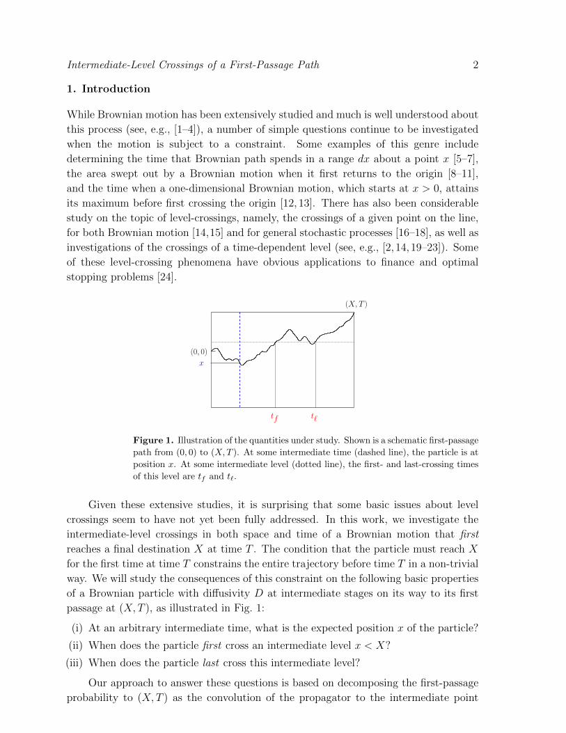
Figure 1. Illustration of the quantities under study. Shown is a schematic first-passage

path from (0, 0) to (X,T ). At some intermediate time (dashed line), the particle is at

position x. At some intermediate level (dotted line), the first- and last-crossing times

of this level are tf and t`.

Given these extensive studies, it is surprising that some basic issues about level

crossings seem to have not yet been fully addressed. In this work, we investigate the

intermediate-level crossings in both space and time of a Brownian motion that first

reaches a final destination X at time T . The condition that the particle must reach X

for the first time at time T constrains the entire trajectory before time T in a non-trivial

way. We will study the consequences of this constraint on the following basic properties

of a Brownian particle with diffusivity D at intermediate stages on its way to its first

passage at (X,T ), as illustrated in Fig. 1:

(i) At an arbitrary intermediate time, what is the expected position x of the particle?

(ii) When does the particle first cross an intermediate level x < X?

(iii) When does the particle last cross this intermediate level?

Our approach to answer these questions is based on decomposing the first-passage

probability to (X,T ) as the convolution of the propagator to the intermediate point

Intermediate-Level Crossings of a First-Passage Path 3

(x, t) and the propagator from this intermediate to the final point. In this framework,

the intermediate crossing properties are simple to formulate; however, the results are

somewhat surprising and depend in an important way on the global nature of the full

first-passage path. In the “ballistic limit”, where X2 � DT , the space-time trajectory

of the first-passage path approaches a straight line. In this case, intermediate-crossing

properties are close to those that arise by treating the first-passage trajectory as purely

ballistic. In the opposite “diffusive limit”, where X2 � DT , the first-passage path is

typically repelled from its final location X so as to avoid hitting X before time T .

Correspondingly, the probability distribution of times for the particle to first cross

an intermediate level 0 < x < X undergoes a transition from unimodality, forX2 � DT ,

to bimodality, for X2 � DT . In the latter case, the first-passage path to (X,T ) is most

likely to cross an intermediate level near the beginning or near the end of its trajectory.

In this bimodal regime, the distribution of the first-crossing times is reminiscent of, but

more singular than, the famous arcsine law [3, 4] for the distribution of times that a

one-dimension Brownian particle spends on one side of the origin.

As a preliminary, we first investigate intermediate crossing phenomena for a purely

Brownian path between (0, 0) and (X,T ) in section 2. In spite of the simplicity of

this problem, the distributions of the first- and last-crossing times of an intermediate

0 < x < X level are also quite rich and have a qualitatively similar unimodal to

bimodal transition as in the case where the trajectory is a first-passage path. Moreover,

the boundary in phase space that demarcates this transition is, surprisingly, not single

valued. In section 3, we investigate intermediate crossing properties when the trajectory

between (0, 0) and (X,T ) is a first-passage path. We briefly discuss the situation where

the intermediate level is negative in section 4. Finally, we offer some perspectives in

section 5.

2. Preliminaries: Intermediate Crossings for Unconstrained Brownian

Motion

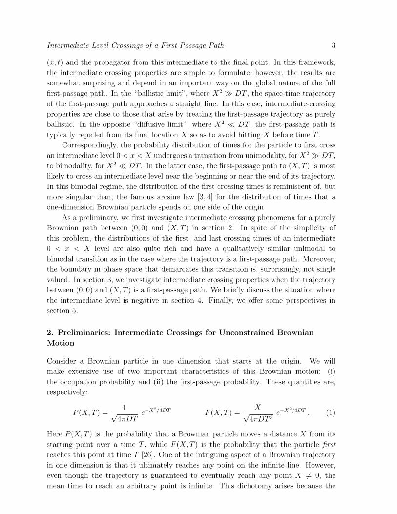
Consider a Brownian particle in one dimension that starts at the origin. We will

make extensive use of two important characteristics of this Brownian motion: (i)

the occupation probability and (ii) the first-passage probability. These quantities are,

respectively:

P (X,T ) =1√

4πDTe−X

2/4DT F (X,T ) =X√

4πDT 3e−X

2/4DT . (1)

Here P (X,T ) is the probability that a Brownian particle moves a distance X from its

starting point over a time T , while F (X,T ) is the probability that the particle first

reaches this point at time T [26]. One of the intriguing aspect of a Brownian trajectory

in one dimension is that it ultimately reaches any point on the infinite line. However,

even though the trajectory is guaranteed to eventually reach any point X 6= 0, the

mean time to reach an arbitrary point is infinite. This dichotomy arises because the

Intermediate-Level Crossings of a First-Passage Path 4

probability that the trajectory first reaches position X at time T asymptotically decays

as T−3/2, from which the mean time to reach X is infinite.

For a Brownian particle that starts at (0, 0) and ends at (X,T ), we now ask: where

is the particle and what is its probability distribution of positions at an earlier time

t < T? The probability that the particle propagates from (0, 0) to (X,T ) may be

written as the convolution of the probabilities for the path from (0, 0) to (x, t) and the

path from (x, t) to the final location (X,T ):

P (X,T ) =

∫P (x, t) P (X−x, T − t) dx

=

∫e−x

2/4Dt

√4πDt

e−(X−x)2/4D(T−t)√

4πD(T−t)dx . (2)

Integrating over to x reproduces, after some simple algebra, P (X, t) in Eq. (1). For

later convenience we introduce the dimensionless time τ = t/T and the dimensionless

length χ=x/X. By maximizing the integrand with respect to x, it is straightforward to

derive that the integrand has its maximum when x = τX. That is, the particle moves a

fraction τ of the final distance in a fraction τ of the total time, a well-known property

of Brownian motion [25].

Finally, we compute the probability P(x, t) that the particle is at x at time t,

given that it is at X at time T . This quantity equals the probability for the subset of

Brownian paths from (0, 0) to (X,T ) that reach x at time t divided by the probability

for all Brownian paths from (0, 0) to (X,T ):

P(x, t) =P (x, t) P (X−x, T−t)

P (X,T )

=e−x

2/4Dt

√4πDt

e−(X−x)2/4D(T−t)√

4πD(T−t)×√

4πDT eX2/4DT

=e−(x−τX)2/4DTτ(1−τ)√

4πDTτ(1− τ)

≡√α

π

e−α(χ−τ)2/τ(1−τ)√

τ(1− τ), (3)

where we have rewritten the last line in terms of χ, τ , and the dimensionless parameter

α = X2/4DT , which demarcates whether the full trajectory is ballistic, for α � 1, or

diffusive, for α� 1.

From Eq. (3), the probability distribution to reach an intermediate point x at

dimensionless time τ is a Gaussian centered at τ = χ whose width√τ(1− τ) is maximal

for τ = 12

and vanishes for τ → 0 and τ → 1. The physical message from these results is

that the average position of a Brownian particle that starts at (0, 0) and ends at (X,T )

interpolates linearly between 0 and X as the time increases from 0 to T [25].

In a similar vein, we now determine when the Brownian particle first crosses and last

crosses an intermediate position x < X, given that the particle is at X (not necessarily

Intermediate-Level Crossings of a First-Passage Path 5

for the first time) at time T . More generally, we compute the probability distributions

for these two events. Using the same reasoning that led to Eq. (3), the probability

F(x, t) that the particle first crosses x at time t is given by:

F(x, t) =F (x, t)P (X − x, T − t)

P (X,T ). (4a)

That is, the first-crossing probability equals the probability for a Brownian particle,

which starts at (0, 0), to first reach (x, t)—hence the factor F (x, t)—times the

probability that the particle propagates from (x, t) to (X,T ), normalized by the

probability for all Brownian paths that propagate from (0, 0) to (X,T ).

Similarly, the probability L(x, t) that the last crossing of x occurs at time t is:

L(x, t) =P (x, t)F (X − x, T − t)

P (X,T ). (4b)

The reasoning that underlies (4b) is slightly more involved than that for (4a). For (x, t)

to be the last crossing, the remaining trajectory must be a time-reversed first-passage

path from (X,T ) to (x, t). This constraint guarantees that the crossing at x is the last

one in the full trajectory to (X,T ).

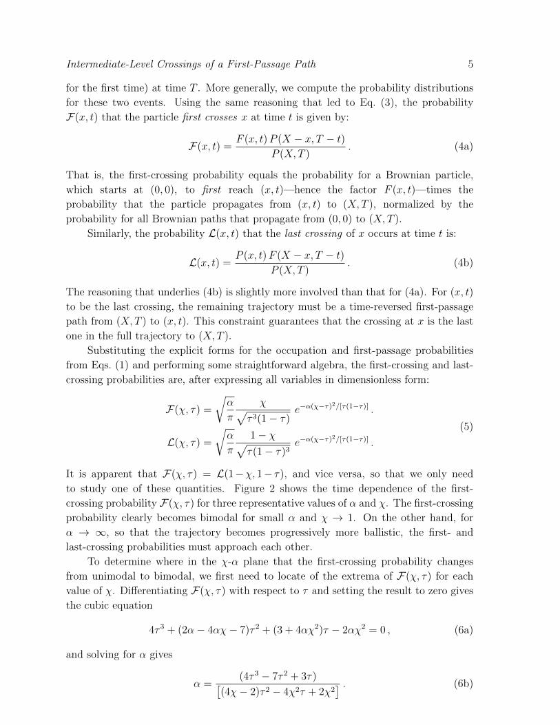
Substituting the explicit forms for the occupation and first-passage probabilities

from Eqs. (1) and performing some straightforward algebra, the first-crossing and last-

crossing probabilities are, after expressing all variables in dimensionless form:

F(χ, τ) =

√α

π

χ√τ 3(1− τ)

e−α(χ−τ)2/[τ(1−τ)] .

L(χ, τ) =

√α

π

1− χ√τ(1− τ)3

e−α(χ−τ)2/[τ(1−τ)] .

(5)

It is apparent that F(χ, τ) = L(1−χ, 1− τ), and vice versa, so that we only need

to study one of these quantities. Figure 2 shows the time dependence of the first-

crossing probability F(χ, τ) for three representative values of α and χ. The first-crossing

probability clearly becomes bimodal for small α and χ → 1. On the other hand, for

α → ∞, so that the trajectory becomes progressively more ballistic, the first- and

last-crossing probabilities must approach each other.

To determine where in the χ-α plane that the first-crossing probability changes

from unimodal to bimodal, we first need to locate of the extrema of F(χ, τ) for each

value of χ. Differentiating F(χ, τ) with respect to τ and setting the result to zero gives

the cubic equation

4τ 3 + (2α− 4αχ− 7)τ 2 + (3 + 4αχ2)τ − 2αχ2 = 0 , (6a)

and solving for α gives

α =(4τ 3 − 7τ 2 + 3τ)[

(4χ− 2)τ 2 − 4χ2τ + 2χ2] . (6b)

Intermediate-Level Crossings of a First-Passage Path 6

100

101

102

α =

1/8

α =

1α

= 8

χ = 0.2 χ = 0.5 χ = 0.8

τ

100

101

α =

1/8

α =

1α

= 8

χ = 0.2 χ = 0.5 χ = 0.8

τ

10-1

100

101

0.0 0.5 1.0

α =

1/8

α =

1α

= 8

χ = 0.2 χ = 0.5 χ = 0.8

τ

α =

1/8

α =

1α

= 8

χ = 0.2 χ = 0.5 χ = 0.8

τ

α =

1/8

α =

1α

= 8

χ = 0.2 χ = 0.5 χ = 0.8

τ

0.5 1.0

α =

1/8

α =

1α

= 8

χ = 0.2 χ = 0.5 χ = 0.8

τ

α =

1/8

α =

1α

= 8

χ = 0.2 χ = 0.5 χ = 0.8

τ

α =

1/8

α =

1α

= 8

χ = 0.2 χ = 0.5 χ = 0.8

τ

0.5 1.0

α =

1/8

α =

1α

= 8

χ = 0.2 χ = 0.5 χ = 0.8

τ

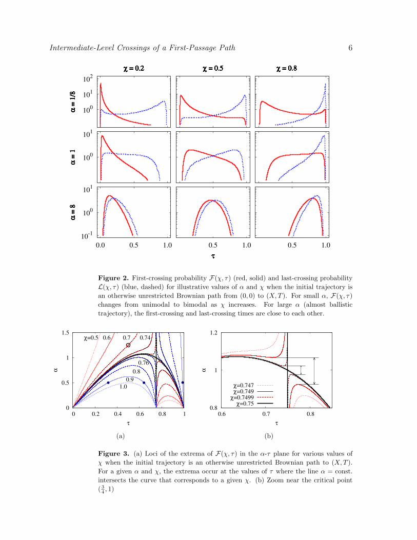
Figure 2. First-crossing probability F(χ, τ) (red, solid) and last-crossing probability

L(χ, τ) (blue, dashed) for illustrative values of α and χ when the initial trajectory is

an otherwise unrestricted Brownian path from (0, 0) to (X,T ). For small α, F(χ, τ)

changes from unimodal to bimodal as χ increases. For large α (almost ballistic

trajectory), the first-crossing and last-crossing times are close to each other.

0

0.5

1

1.5

0 0.2 0.4 0.6 0.8 1

α

τ

χ=0.5 0.6 0.7 0.74

0.76

0.8

0.9

1.0

(a)

0.8

1

1.2

0.6 0.7 0.8

α

τ

χ=0.747

χ=0.749

χ=0.7499

χ=0.75

(b)

Figure 3. (a) Loci of the extrema of F(χ, τ) in the α-τ plane for various values of

χ when the initial trajectory is an otherwise unrestricted Brownian path to (X,T ).

For a given α and χ, the extrema occur at the values of τ where the line α = const.

intersects the curve that corresponds to a given χ. (b) Zoom near the critical point

( 34 , 1)

Intermediate-Level Crossings of a First-Passage Path 7

These loci for α are plotted as a function of τ for various values of χ in Fig. 3(a). For

given α and χ, the extrema occur at the τ values where the line α = const. intersects

the branches of the curve for a given χ. For example, in Fig. 3(a), when α = 0.5 and

χ = 0.9, F has three extrema at τ = 0.32, 0.64, and 0.99, as indicated by the dots. On

the other hand for α = 1.25 and χ = 0.7, there is a single extremum (circle). When

χ ≈ 0.75, the regime of bimodality extends over the widest range of α.

0

0.25

0.5

0.75

1

0 0.2 0.4 0.6 0.8 1

α

χ

unimodal

a

b

bimodal

c

(a)

0.8

0.9

1

1.1

0.745 0.7475 0.75 0.7525

α

χ

unimodal

b e

bimodal

d

(b)

Figure 4. (a) Phase diagram, showing the domains in the parameter space where

the first-crossing probability is unimodal and where it is bimodal for an unrestricted

Brownian path from (0, 0) to (X,T ). The points marked a, b, c are at (0, 72 −2√

3),

(0.747835 · · · , 1.09325 . . .), and (1, 12 ), respectively. (b) Detail near the cusp in the

phase boundary; the points marked d, e are at ( 34 , 1) and ( 3

4 , 4(2−√

3)), respectively.

The behavior near the critical point (τ, α) = (34, 1) is particularly intriguing

(Fig. 3(b)). For a given value of χ that is less than but very close to χ = 3/4, there are

two distinct sets of solutions—one set with α slightly less than 1 and another set with

α slightly larger than 1. There is also a small gap between these two solution sets, as

indicated in Fig. 3(b) for the cases χ = 0.749 and χ = 0.7499. The consequence of this

feature is that the unimodal to bimodal phase boundary is not single valued near the

cusp, as shown in Fig. 4. It is quite remarkable that such a simple question about a

Brownian path—namely the time for the path to cross an intermediate position—leads

to such a rich phenomenon.

3. Intermediate Crossings for First-Passage Paths

We now turn to the properties of intermediate crossings for first-passage paths, where

the first-passage constraint for the full trajectory from (0, 0) to (X,T ) significantly

affects the global nature of intermediate trajectory and concomitantly, the intermediate

crossings. We divide our discussion into: (i) the location of the particle at an arbitrary

intermediate time and (ii) the time when the particle crosses an arbitrary intermediate

position.

Intermediate-Level Crossings of a First-Passage Path 8

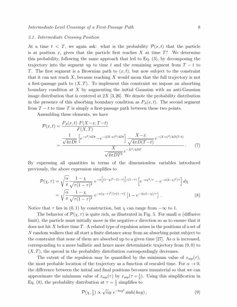
3.1. Intermediate Crossing Position

At a time t < T , we again ask: what is the probability P(x, t) that the particle

is at position x, given that the particle first reaches X at time T? We determine

this probability, following the same approach that led to Eq. (3), by decomposing the

trajectory into the segment up to time t and the remaining segment from T − t to

T . The first segment is a Brownian path to (x, t), but now subject to the constraint

that it can not reach X, because reaching X would mean that the full trajectory is not

a first-passage path to (X,T ). To implement this constraint we impose an absorbing

boundary condition at X by augmenting the initial Gaussian with an anti-Gaussian

image distribution that is centered at 2X [3,26]. We denote the probability distribution

in the presence of this absorbing boundary condition as PA(x, t). The second segment

from T − t to time T is simply a first-passage path between these two points.

Assembling these elements, we have

P(x, t) =PA(x, t) F (X−x, T−t)

F (X,T )

=

1√4πDt

[e−x

2/4Dt−e−(2X−x)2/4Dt] X−x√

4πD(T−t)e−(X−x)

2/4D(T−t)

X√4πDT 3

e−X2/4DT

. (7)

By expressing all quantities in terms of the dimensionless variables introduced

previously, the above expression simplifies to

P(χ, τ) =

√α

π

1− χ√τ(1− τ)3

e−α[(1−χ)2−(1−τ)

]/(1−τ)

[e−αχ

2/τ − e−α(2−χ)2/τ]dχ

=

√α

π

1− χ√τ(1− τ)3

e−α(χ−τ)2/[τ(1−τ)] [1− e−4α(1−χ)/τ] . (8)

Notice that τ lies in (0, 1) by construction, but χ can range from −∞ to 1.

The behavior of P(χ, τ) is quite rich, as illustrated in Fig. 5. For small α (diffusive

limit), the particle must initially move in the negative-x direction so as to ensure that it

does not hit X before time T . A related type of repulsion arises in the positions of a set of

N random walkers that all start a finite distance away from an absorbing point subject to

the constraint that none of them are absorbed up to a given time [27]. As α is increased,

corresponding to a more ballistic and hence more deterministic trajectory from (0, 0) to

(X,T ), the spread in the probability distribution correspondingly decreases.

The extent of the repulsion may be quantified by the minimum value of xmp(τ),

the most probable location of the trajectory as a function of rescaled time. For α→ 0,

the difference between the initial and final positions becomes immaterial so that we can

approximate the minimum value of xmp(τ) by xmp(τ = 12). Using this simplification in

Eq. (8), the probability distribution at τ = 12

simplifies to

P(χ, 12) ∝ √αy e−4αy2 sinh(4αy) , (9)

Intermediate-Level Crossings of a First-Passage Path 9

-2

-1

0

1

0 0.5 1

χ

τ

α = 1/32 α = 1 α = 32

0.5 1

χ

τ

α = 1/32 α = 1 α = 32

0.5 1

χ

τ

α = 1/32 α = 1 α = 32

Figure 5. Heatmaps of the conditional occupation probability P(χ, τ) for a first-

passage path from (0, 0) to (X,T ) for illustrative values of α in the τ -χ plane.

The smooth curve shows the time dependence of the most probable location of the

particle. For small α, the trajectory is initially repelled from its final destination. The

distribution is most diffuse near τ = 12 and most localized near τ = 0 and τ = 1.

where y = χ− 1. Finding the maximum of this latter expression is now elementary and

we find that for α→ 0, the minimum on the most probable trajectory is located at

y∗ ' − 1

2√α.

Thus for α → 0, the most probable trajectory is strongly repelled from the final point

for τ < 1/2 and subsequently is strongly attracted to this final point.

3.2. Intermediate Crossing Times

Parallel to the discussion given for the pure Brownian path, we now compute the

distribution of times when the first-passage trajectory to (X,T ) crosses an arbitrary

intermediate level. We separately consider the cases of the first crossing and the last

crossing because the calculational details and the results for these two cases are quite

different.

3.2.1. First-crossing probability As in the case where the full trajectory is an

unconstrained Brownian path that starts at (0, 0) and ends at (X,T ), we decompose

the trajectory into an initial segment that starts at (0, 0) and crosses x for the first time

at time t, and a final segment that starts at (x, t) and crosses X for the first time at

time T . Here the analog of Eq. (4a) is

F(x, t) =F (x, t)F (X − x, T − t)

F (X,T ). (10)

Intermediate-Level Crossings of a First-Passage Path 10

We now substitute the relevant first-passage probabilities from (1) into the above

equation to obtain

F(x, t) =|x|√

4πDt3e−x

2/4Dt |X − x|√4πD(T − t)3

e−(X−x)2/4D(T−t)

/|X|√

4πDT 3e−X

2/4DT .

(11)

In terms of the dimensionless variables α, χ, and τ , the above expression simplifies, after

some straightforward algebra, to

F(χ, τ) =

√α

π

|1− χ| |χ|[(1− τ)τ

]3/2 e−α(τ−χ)2/[τ(1−τ)] . (12)

100

101

102

α =

1/8

α =

1α

= 8

χ = 0.2 χ = 0.5 χ = 0.8

τ

100

101

α =

1/8

α =

1α

= 8

χ = 0.2 χ = 0.5 χ = 0.8

τ

10-1

100

101

0.0 0.5 1.0

α =

1/8

α =

1α

= 8

χ = 0.2 χ = 0.5 χ = 0.8

τ

α =

1/8

α =

1α

= 8

χ = 0.2 χ = 0.5 χ = 0.8

τ

α =

1/8

α =

1α

= 8

χ = 0.2 χ = 0.5 χ = 0.8

τ

0.5 1.0

α =

1/8

α =

1α

= 8

χ = 0.2 χ = 0.5 χ = 0.8

τ

α =

1/8

α =

1α

= 8

χ = 0.2 χ = 0.5 χ = 0.8

τ

α =

1/8

α =

1α

= 8

χ = 0.2 χ = 0.5 χ = 0.8

τ

0.5 1.0

α =

1/8

α =

1α

= 8

χ = 0.2 χ = 0.5 χ = 0.8

τ

Figure 6. First-crossing probability F(χ, τ) (red, solid) and the last-crossing

probability L(χ, τ) (blue, dashed) for illustrative values of α and χ when the initial

trajectory is a first-passage path from (0, 0) to (X,T ). For small α, F(χ, τ) is bimodal

while L(χ, τ) is unimodal and sharply peaked as τ → 1. For large α (almost ballistic

trajectory), the first-crossing and last-crossing times nearly coincide.

Once again, the qualitative behavior of this first-crossing probability depends in an

essential way on the value of α (Fig. 6). For large α (ballistic limit) F(χ, τ) is sharply

peaked about the point τ = χ. Thus in this ballistic limit, the most probable time

for a Brownian particle to first reach a distance x is simply equal to x. Moreover, the

distribution in (12) reduces to a Gaussian form for χ ≈ τ .

Intermediate-Level Crossings of a First-Passage Path 11

Conversely, in the diffusive limit of α → 0, and for τ � α and 1 − τ � α

(i.e., τ not too close to 0 or 1), the probability density function is controlled by the

factor[τ(1 − τ)

]−3/2, which is similar to, but more singular than the arcsine law [4].

The surprising result for this limit is that a Brownian particle is most likely to cross

an arbitrary intermediate level either at the very beginning or at the very end of its

trajectory.

1−τ

(X,T )

(0, 0)(a)

(X,T )

(0, 0)(b)

χ

τ

1−χ

Figure 7. (a) A first-passage path that consists of a solid and dashed segment with a

first-crossing at (χ, τ). Interchanging the order of these segments gives a first-crossing

at (1−χ, 1−τ).

A remarkable aspect of the first-crossing probability (12) is its invariance under the

simultaneous interchanges τ → 1−τ and χ → 1−χ. We can give a simple graphical

argument to justify this symmetry (Fig. 7). In (a), a first-passage path from (0, 0)

to (X,T ) is comprised of a first crossing (dashed) to (χ, τ) (in scaled units) and the

remaining segment to (X,T ) (solid). Interchanging these two segments leads to a first-

crossing segment to (1−χ, 1− τ) and the remaining segment to (X,T ). Since the

segments are independent, the probability for these two first-passage paths in the figure

are identical and thus F(χ, τ) = F(1−χ, 1−τ).

(b)

(0, 0) (0, 0)

(X,T )(X,T )

(a)

Figure 8. (a) First-passage paths that first cross an intermediate level near τ = 0 or

τ = 1 on an exaggerated scale to emphasize the limit α� 1. (b) A first-passage path

that first crosses the intermediate level near τ = 12 .

We can apply this same perspective to argue that F is bimodal for α� 1. Indeed,

let us compare a first-passage path to the final point that has its first crossing close to

τ = 0 or τ = 1, and a first-passage path that has its first crossing near τ = 1/2. In the

former case (see Fig. 8(a)), the remainder of the path away from the first crossing must

be repelled from the final point. The probability for such a first-passage path from (0, 0)

to (X,T ) scales as T−3/2 for α� 1. On the other hand, the probability for a path that

Intermediate-Level Crossings of a First-Passage Path 12

first-crosses χ near T/2 is the product of the probabilities of two first-passage paths of

duration T/2, namely(T−3/2/2

)2, which is much less than T−3/2. Thus a first-crossing

near T/2 is unlikely for α� 1.

To determine where in the phase space the transition in F between unimodality and

bimodality occurs, we again determine the extrema of F . Following the same procedure

that led to Eq. (6), we obtain the cubic equation for the location of the extrema

6τ 3 + (2α− 4αχ− 9)τ 2 + (3 + 4αχ2)τ − 2αχ2 = 0 ,

and the resulting solutions for α are plotted as a function of τ for various values of

χ in Fig. 9(a). For given α and χ, the extrema occur at the τ values where the line

α = const. intersects the curve corresponding to a given χ. Figure 9(b) shows the region

of the phase diagram where the first-crossing probability is unimodal and where it is

bimodal. As a result of the symmetry of F , the phase diagram is symmetric about the

point χ = 12.

0

1

2

0 0.2 0.4 0.6 0.8 1

α

τ

χ=0.0

0.2

0.4

0.490.51

0.6

0.8

1.0

(a)

0

0.5

1

1.5

0 0.2 0.4 0.6 0.8 1

α

χ

unimodal

a

b

bimodal c

(b)

Figure 9. (a) Loci of the extrema of F(χ, τ) in the α-τ plane for various values of χ

when the initial trajectory is a first-passage path to (X,T ). For a given α and χ, the

extrema occur at the values of τ where the line α = const. intersects the curve that

corresponds to a given χ. (b) Phase diagram, showing where in the parameter space

the first-crossing probability, for a a first-passage Brownian path from (0, 0) to (X,T ),

is unimodal and where it is bimodal. The points marked a, b, c are at (0, 92 − 3√

2),

( 12 ,

32 ), and (1, 92 − 3

√2), respectively.

3.2.2. Last-crossing probability We now determine when the particle crosses a specified

intermediate level for the last time. In principle, we may perform this calculation by

decomposing the trajectory into an initial segment from (0, 0) to the last crossing of

x at time t, and a remaining first-passage segment from (x, t) to (X,T ). The subtle

feature here is that this second segment must also obey the constraint that this segment

always remains greater than x, so that no additional crossings of x occur after time t.

To satisfy the latter condition, we must also impose an absorbing boundary condition

at x. Thus the particle begins the second segment at the absorbing boundary, so that

Intermediate-Level Crossings of a First-Passage Path 13

the first-passage probability to (X,T ) would equal zero. To sidestep this pathology, we

could start the particle at x+dx and take the limit dx at the end of the calculation. This

limiting process is a delicate, however, and we therefore give an alternative approach

that avoids any limiting processes. The price, however, is the necessity to break the

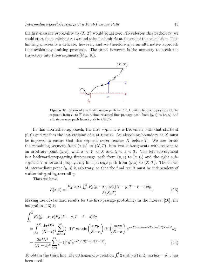
trajectory into three segments (Fig. 10).

t`

y

sx

(X,T )

Figure 10. Zoom of the first-passage path in Fig. 1, with the decomposition of the

segment from t` to T into a time-reversed first-passage path from (y, s) to (x, t`) and

a first-passage path from (y, s) to (X,T ).

In this alternative approach, the first segment is a Brownian path that starts at

(0, 0) and reaches the last crossing of x at time t`. An absorbing boundary at X must

be imposed to ensure that this segment never reaches X before T . We now break

the remaining segment from (x, t`) to (X,T ), into two sub-segments with respect to

an arbitrary point (y, s), with x < Y < X and t` < s < T . The left sub-segment

is a backward-propagating first-passage path from (y, s) to (x, t`) and the right sub-

segment is a forward-propagating first-passage path from (y, s) to (X,T ). The choice

of intermediate point (y, s) is arbitrary, so that the final result must be independent of

s after integrating over all y.

Thus we have

L(x, t) =PA(x, t)

∫ XxFA(y − x, s)FA(X − y, T − t− s)dy

F (X,T ). (13)

Making use of standard results for the first-passage probability in the interval [26], the

integral in (13) is∫ X

x

FA(y − x, x)FA(X − y, T − t− s)dy

=

∫ X

x

4π2D2

(X−x)4

∞∑m,n=1

(−1)mnm sin

(nπy

X−x

)sin

(mπy

X−x

)e−π

2D[n2s+m2(T−t−s)]/(X−x)2dy

=2π2D2

(X − x)3

∞∑n=1

(−1)nn2e−n2π2D(T−t)/(X−x)2 . (14)

To obtain the third line, the orthogonality relation∫ 1

02 sin(nπx) sin(mπx)dx = δmn has

been used.

Intermediate-Level Crossings of a First-Passage Path 14

0

2

4

6

8

10

0 0.2 0.4 0.6 0.8 1

F(χ

, τ)

τ

α = 1/16α = 1/4α = 1α = 4α = 16

(a)

0

2

4

6

8

10

0 0.2 0.4 0.6 0.8 1

L(χ

, τ)

τ

α = 1/16α = 1/4α = 1α = 4α = 16

(b)

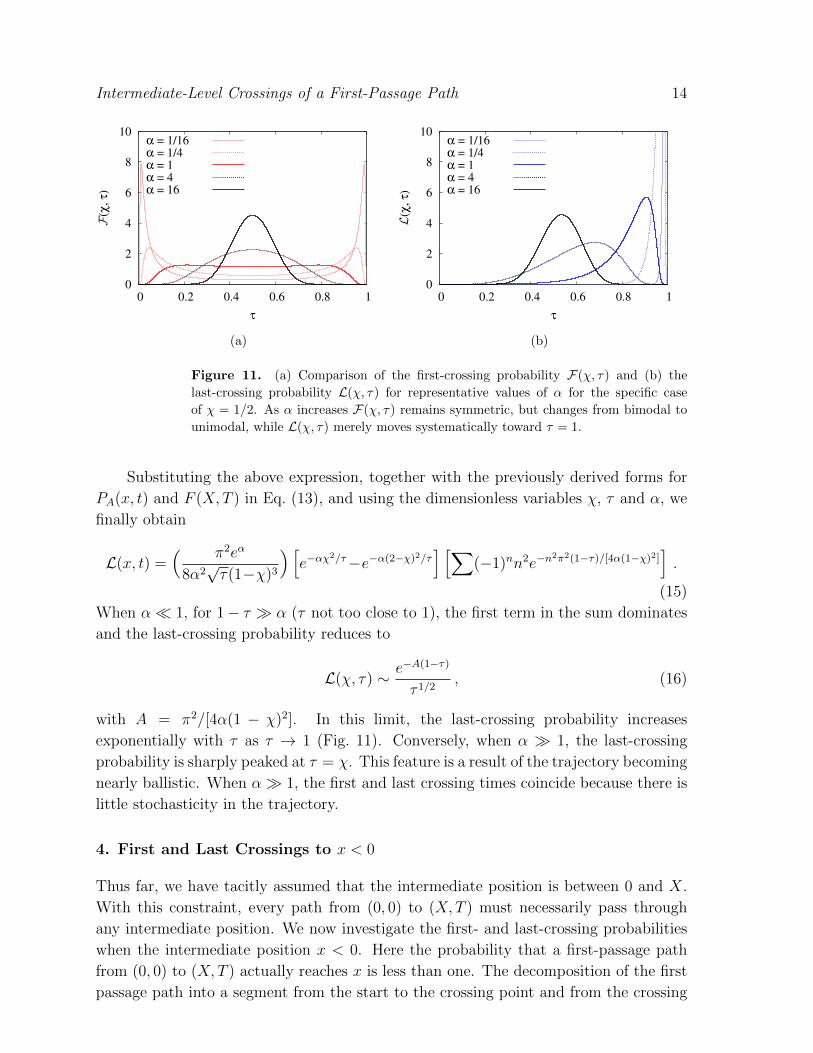
Figure 11. (a) Comparison of the first-crossing probability F(χ, τ) and (b) the

last-crossing probability L(χ, τ) for representative values of α for the specific case

of χ = 1/2. As α increases F(χ, τ) remains symmetric, but changes from bimodal to

unimodal, while L(χ, τ) merely moves systematically toward τ = 1.

Substituting the above expression, together with the previously derived forms for

PA(x, t) and F (X,T ) in Eq. (13), and using the dimensionless variables χ, τ and α, we

finally obtain

L(x, t) =( π2eα

8α2√τ(1−χ)3

) [e−αχ

2/τ−e−α(2−χ)2/τ] [∑

(−1)nn2e−n2π2(1−τ)/[4α(1−χ)2]

].

(15)

When α� 1, for 1− τ � α (τ not too close to 1), the first term in the sum dominates

and the last-crossing probability reduces to

L(χ, τ) ∼ e−A(1−τ)

τ 1/2, (16)

with A = π2/[4α(1 − χ)2]. In this limit, the last-crossing probability increases

exponentially with τ as τ → 1 (Fig. 11). Conversely, when α � 1, the last-crossing

probability is sharply peaked at τ = χ. This feature is a result of the trajectory becoming

nearly ballistic. When α� 1, the first and last crossing times coincide because there is

little stochasticity in the trajectory.

4. First and Last Crossings to x < 0

Thus far, we have tacitly assumed that the intermediate position is between 0 and X.

With this constraint, every path from (0, 0) to (X,T ) must necessarily pass through

any intermediate position. We now investigate the first- and last-crossing probabilities

when the intermediate position x < 0. Here the probability that a first-passage path

from (0, 0) to (X,T ) actually reaches x is less than one. The decomposition of the first

passage path into a segment from the start to the crossing point and from the crossing

Intermediate-Level Crossings of a First-Passage Path 15

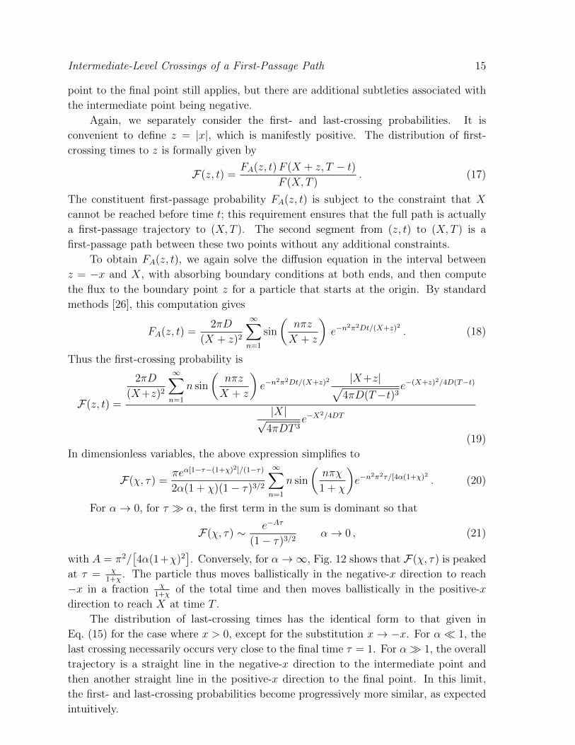
point to the final point still applies, but there are additional subtleties associated with

the intermediate point being negative.

Again, we separately consider the first- and last-crossing probabilities. It is

convenient to define z = |x|, which is manifestly positive. The distribution of first-

crossing times to z is formally given by

F(z, t) =FA(z, t)F (X + z, T − t)

F (X,T ). (17)

The constituent first-passage probability FA(z, t) is subject to the constraint that X

cannot be reached before time t; this requirement ensures that the full path is actually

a first-passage trajectory to (X,T ). The second segment from (z, t) to (X,T ) is a

first-passage path between these two points without any additional constraints.

To obtain FA(z, t), we again solve the diffusion equation in the interval between

z = −x and X, with absorbing boundary conditions at both ends, and then compute

the flux to the boundary point z for a particle that starts at the origin. By standard

methods [26], this computation gives

FA(z, t) =2πD

(X + z)2

∞∑n=1

sin

(nπz

X + z

)e−n

2π2Dt/(X+z)2 . (18)

Thus the first-crossing probability is

F(z, t) =

2πD

(X+z)2

∞∑n=1

n sin

(nπz

X + z

)e−n

2π2Dt/(X+z)2 |X+z|√4πD(T−t)3

e−(X+z)2/4D(T−t)

|X|√4πDT 3

e−X2/4DT

(19)

In dimensionless variables, the above expression simplifies to

F(χ, τ) =πeα[1−τ−(1+χ)

2]/(1−τ)

2α(1 + χ)(1− τ)3/2

∞∑n=1

n sin

(nπχ

1 + χ

)e−n

2π2τ/[4α(1+χ)2 . (20)

For α→ 0, for τ � α, the first term in the sum is dominant so that

F(χ, τ) ∼ e−Aτ

(1− τ)3/2α→ 0 , (21)

with A = π2/[4α(1+χ)2

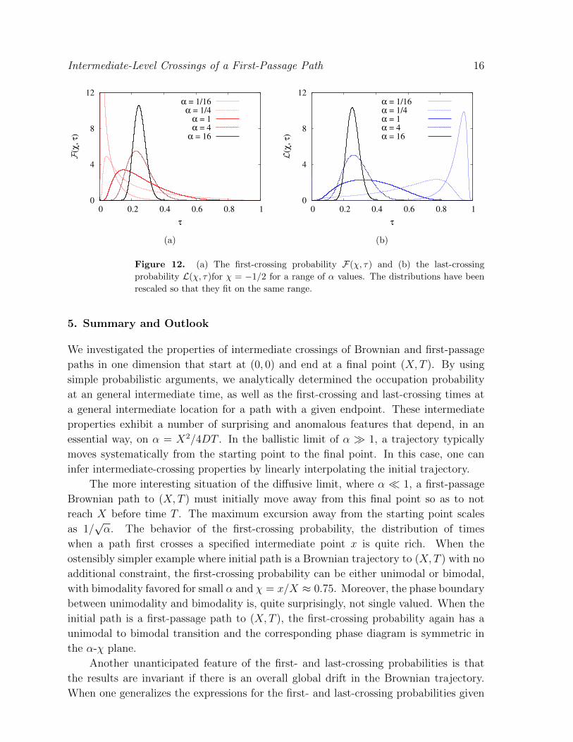
]. Conversely, for α→∞, Fig. 12 shows that F(χ, τ) is peaked

at τ = χ1+χ

. The particle thus moves ballistically in the negative-x direction to reach

−x in a fraction χ1+χ

of the total time and then moves ballistically in the positive-x

direction to reach X at time T .

The distribution of last-crossing times has the identical form to that given in

Eq. (15) for the case where x > 0, except for the substitution x→ −x. For α� 1, the

last crossing necessarily occurs very close to the final time τ = 1. For α� 1, the overall

trajectory is a straight line in the negative-x direction to the intermediate point and

then another straight line in the positive-x direction to the final point. In this limit,

the first- and last-crossing probabilities become progressively more similar, as expected

intuitively.

Intermediate-Level Crossings of a First-Passage Path 16

0

4

8

12

0 0.2 0.4 0.6 0.8 1

F(χ

, τ)

τ

α = 1/16α = 1/4

α = 1α = 4

α = 16

(a)

0

4

8

12

0 0.2 0.4 0.6 0.8 1

L(χ

, τ)

τ

α = 1/16α = 1/4α = 1α = 4α = 16

(b)

Figure 12. (a) The first-crossing probability F(χ, τ) and (b) the last-crossing

probability L(χ, τ)for χ = −1/2 for a range of α values. The distributions have been

rescaled so that they fit on the same range.

5. Summary and Outlook

We investigated the properties of intermediate crossings of Brownian and first-passage

paths in one dimension that start at (0, 0) and end at a final point (X,T ). By using

simple probabilistic arguments, we analytically determined the occupation probability

at an general intermediate time, as well as the first-crossing and last-crossing times at

a general intermediate location for a path with a given endpoint. These intermediate

properties exhibit a number of surprising and anomalous features that depend, in an

essential way, on α = X2/4DT . In the ballistic limit of α � 1, a trajectory typically

moves systematically from the starting point to the final point. In this case, one can

infer intermediate-crossing properties by linearly interpolating the initial trajectory.

The more interesting situation of the diffusive limit, where α � 1, a first-passage

Brownian path to (X,T ) must initially move away from this final point so as to not

reach X before time T . The maximum excursion away from the starting point scales

as 1/√α. The behavior of the first-crossing probability, the distribution of times

when a path first crosses a specified intermediate point x is quite rich. When the

ostensibly simpler example where initial path is a Brownian trajectory to (X,T ) with no

additional constraint, the first-crossing probability can be either unimodal or bimodal,

with bimodality favored for small α and χ = x/X ≈ 0.75. Moreover, the phase boundary

between unimodality and bimodality is, quite surprisingly, not single valued. When the

initial path is a first-passage path to (X,T ), the first-crossing probability again has a

unimodal to bimodal transition and the corresponding phase diagram is symmetric in

the α-χ plane.

Another unanticipated feature of the first- and last-crossing probabilities is that

the results are invariant if there is an overall global drift in the Brownian trajectory.

When one generalizes the expressions for the first- and last-crossing probabilities given

Intermediate-Level Crossings of a First-Passage Path 17

in Eqs. (4), (10), and (13) to incorporate a constant drift, all factors that involve the

drift velocity cancel out. It would be worthwhile to understand the full ramifications of

this simple observation.

Finally, it is worth mentioning that the decomposition of the first-passage path

in (10) provides the starting point for efficient simulations of intermediate crossing

phenomena. The naive way to numerically determine intermediate crossing properties

is by direct simulation of a random walk in which the times at which various

intermediate positions are reached are recorded for a walk that reaches a given final

point. From this data, one can reconstruct the first-crossing (as well as the last-

crossing) probabilities. As a much more efficient alternative, one can first select a set of

intermediate positions and then directly move a particle only between these intermediate

positions. Correspondingly, the time between each of these macro-steps is incremented

from the appropriate distribution of first passage times. This procedure can be made

still more efficient by only allowing the walk to move to intermediate positions that are

progressively closer to the final position. Thus arbitrarily long random walks can be

simulated with a finite number of steps.

We thank Satya Majumdar for helpful suggestions and literature advice. Financial

support for this research was provided in part by grant No. 2012145 from the United

States-Israel Binational Science Foundation (BSF) and Grant No. DMR-1205797 from

the National Science Foundation.

Intermediate-Level Crossings of a First-Passage Path 18

6. References

[1] P. Levy, Compositio Math. 7, 283 (1939).

[2] P. Levy Processus stochastiques et mouvement brownien 2nd ed. Gauthier-Villars, Paris 1965),

[3] W. Feller, An Introduction to Probability Theory and its Applications (John Wiley and Sons, New

York, 1968).

[4] P. Morters and Y. Peres, Brownian Motion (Cambridge University Press, Cambridge, UK, 2010).

[5] D. A. Darling and M. Kac, Trans. Amer. Math. Soc. 84, 444 (1957).

[6] D. Ray, Illinois J. Math. 7, 615 (1963).

[7] F. B. Knight, Trans. Amer. Math. Soc. 109, 56 (1963).

[8] K. L. Chung, Bull. Amer. Math. Soc. 81, 742 (1975).

[9] K. L. Chung, Arkiv fur Matematik, 14, 155 (1976)

[10] S. N. Majumdar and A. Comtet, Phys. Rev. Lett. 92, 225501 (2004).

[11] S. N. Majumdar and A. Comtet, J. Stat. Phys. 119, 777 (2005).

[12] J. Randon-Furling and S. N. Majumdar, J. Stat. Mech. P10008, (2007).

[13] S. N. Majumdar, J. Randon-Furling, M. J. Kearney, and M. Yor, J. Phys. A: Mathematical and

Theoretical 41, 365005 (2008).

[14] M. Abundo, Stat. Probab. Lett. 58, 131 (2002).

[15] J. Bertoin, Probab. Theory Relat. Fields 117, 289 (2000).

[16] M. F. Kratz, Probab. Surv. 3, 230 (2006).

[17] J. Pitman and M. Yor, Ann. Probab. 11, 780 (1986).

[18] R. J. Adler, G. Samorodnitsky, and T. Gadrich, Ann. Appl. Probab. 3, 2, 553 (1993).

[19] H. R. Lerche, Lecture Notes in Statistics vol. 40, (Springer-Verlag, Berlin, 1986).

[20] L. Breiman, Proc. Fifth Berkeley Symp. on Math. Statist. and Prob. Vol. 2, Pt. 2 (Univ. of Calif.

Press, 1967), 9–16.

[21] P. Groeneboom, Probab. Theory Related Fields 81, 79 (1989).

[22] A. Novikov, V. Frishling, and N. Kordzakhia, J. Appl. Probab. 36, 1019 (1999).

[23] H. E. Daniels, Bernoulli, 64, 571 (2000).

[24] S. N. Majumdar and J.-P. Bouchaud, Quant. Fin. 8, 753 (2008).

[25] M. L. Eaton, Multivariate Statistics: a Vector Space Approach (John Wiley & Sons, New York,

1983) pp. 116–117.

[26] S. Redner, A Guide to First-Passage Processes, (Cambridge University Press, Cambridge, UK,

2001).

[27] B. Meerson and S. Redner, J. Stat. Mech. P08008 (2014).

[28] D. A. Darling and A. J. F. Siegert, Ann. Math. Stat. 24, 624 (1953).