Interference Simulator for the Whole HF Band: Application to CW-Morse

IEEE TRANSACTIONS ON ELECTROMAGNETIC COMPATIBILITY, VOL. 56, NO. 3, JUNE 2014 571

Interference Simulator for the Whole HF Band:Application to CW-Morse

Eduardo Mendieta-Otero, Ivan A. Perez-Alvarez, Member, IEEE, and Baltasar Perez-Dıaz

Abstract—In this paper, we use jointly a model of narrow bandinterference and a congestion model to model and implement aninterference simulator for the whole HF band. The result is a modelto generate interfering signals that could be found in a given fre-quency allocation, at a given time (past, present, or future) and fora given location. Our model does not require measurements and itis characterized by its ease of use and the freedom it offers to choosescene (modulation, location, week, year, etc.). In addition, we havedefined a generic modulating function and the conditions to modela “contact” continuous wave (CW)-Morse, which meets the usualstandards of contest. Consequently, our interference model in con-junction with the CW-Morse modulating function designed resultsin a specific CW-Morse model for amateur contests. As an exampleof the simulation model, we simulate the CW-Morse communica-tions on the contest “ARRL Field Day 2011.”

Index Terms—Congestion, continuous wave (CW)-Morse, inter-ference, Poisson processes.

I. INTRODUCTION

THE present needs for more accurate modeling and sim-ulation of the HF band (formally, 3–30 MHz [1]) have

motivated the development of wideband models and their imple-mentation in wideband channel simulators. For example, thereis a need for modeling the HF channel bandwidth to assist inthe development of systems based on the recently promulgatedUS military standard MIL-STD-188-110C that contains anappendix (Appendix D) defining a new family of widebandHF data waveforms. Moreover, fully realizing the potential ofthese new waveforms will require enhanced capabilities in otherelements of HF communications systems such as automatic linkestablishment systems.

While propagation conditions have been studied extensivelyover several decades, there are relatively fewer published stud-ies that have looked at noise and interference in the HF band.Moreover, it is a well-known fact that interference from legit-imate users is one of the most common problems encountered

Manuscript received September 10, 2012; revised May 6, 2013 and October23, 2013; accepted February 23, 2014. Date of publication April 7, 2014; date ofcurrent version May 19, 2014. This work was supported in part by the Ministeriode Economıa y Competitividad under Grant TEC2010-21217-C02-01.

E. Mendieta-Otero and I. A. Perez-Alvarez are with the Institute for Techno-logical Development and Innovation in Communications, Las Palmas de GranCanaria, Las Palmas 35017, Spain and also with the Department of Signals andCommunications, Las Palmas de Gran Canaria University, Las Palmas 35017,Spain (e-mail: [email protected]; [email protected]).

B. Perez-Dıaz is with the Institute for Technological Development and In-novation in Communications, Las Palmas de Gran Canaria, Las Palmas 35017,Spain (e-mail: [email protected]).

Digital Object Identifier 10.1109/TEMC.2014.2313064

in the use of the HF spectrum. For the radio amateur serviceseveral frequency bands are allocated [2] and [3, p. 982], andproperly licensed stations are permitted to operate at any fre-quency within these bands. It is remarkable that in the 2000sthere were about three million amateur radio operators world-wide [4]. Given the global scope and the rules of participation [5]of major radio amateur contests (ARRL Field Day, ARRL Inter-national DX Contest, IARU HF Championship, CQ WorldWideContest, etc.), it is reasonable to expect:

1) a high number of contestants; and2) at reception, a wide range of values for: the powers, the

frequencies, the start times of communications, etc.Thus, the major radio amateur contests can be a good scene to

evaluate a communications system subjected to a high degree of“interferences.” Also, interference from other users is frequentlymore important than the man-made noise [6] from incidentalradiators or atmospheric noise from lightning [7].

Therefore, for the evaluation of HF equipment in general, andwideband systems in particular, comes the need for interferencesimulators throughout the HF band. If in addition, the simulatoris capable of generating interference in a temporary situation orin any location, the simulations for the situation in the past couldserve as a benchmark to the own simulator in its most desirableapplication: generating interference in a future environment.With this objective, we use jointly a model of narrow bandinterference and a congestion model to generate a new modeland implement an interference simulator for the whole HF band.The congestion value indicates the probability of interferenceunder the given conditions [3].

Communication methods of radio amateurs are diverse.However, we have focused our attention on continuous wave(CW)-Morse. Its principle of operation is based on the carrier-no carrier signal, which means a great simplicity in the hardwareimplementation, essential in emergency situations. With regardto its ability to interfere, CW is a signal that focuses all itsenergy in a very narrow bandwidth. However, our simulatoropens the possibility of implementing any type of modulation.The “ARRL Field Day 2011,” organized by the American RadioRelay League (ARRL), is used as application example of thesimulator.

As previous models in the same line that ours, wehave found [8], [9], and [10]. The main difference of themodel in [8] and [9] with ours is that in our model theamplitudes of interference are deduced from a model ofcongestion [3] and in [8] and [9] are deduced from a model de-veloped by Hall [11]. Basically, the congestion model electionhas been made to have the capability of extrapolation in time inour model and in our simulator. Our model and the model in [10]

0018-9375 © 2014 IEEE. Personal use is permitted, but republication/redistribution requires IEEE permission.See http://www.ieee.org/publications standards/publications/rights/index.html for more information.

572 IEEE TRANSACTIONS ON ELECTROMAGNETIC COMPATIBILITY, VOL. 56, NO. 3, JUNE 2014

use a model of congestion to deduce the amplitudes of the inter-ference. However, the main differences of our model with thatof [10] are: 1) the model of [10] does not include modulation;2) in [10], the number of interferences and the frequencies ofthe interference, are fixed: 800 sine waves 250 Hz apart, givinga total bandwidth of 200 kHz. In our model, the number andfrequency of interference are random variables (RVs) limitedby the event one wishes to simulate.

This paper is organized as follows. Section II describes amodel of narrow band interference that is the fundamental struc-ture of our model of interference: a sum of sinusoids. Section IIIdescribes our interference model for the whole HF band (1.606–30 MHz). This is the frequency range of our model of interfer-ence since it is the frequency range of the congestion modelthat we used in our model. Section IV describes a model ofcongestion from which we deduce, in our model, the values ofamplitude of the interference. Section V: 1) clarifies how theseamplitudes are deduced; 2) develops the modulation chosen tothe interference; 3) presents the application example chosen,the “ARRL Field Day 2011”; 4) describes the temporal controlprocesses (onset, duration, etc.) of interference of our model.Section VI describes the implementation of our simulator basedon our model. Section VII exposes the simulation results for theselected example of application, the “ARRL Field Day 2011,”at a given time and place. Section VIII presents future work.Section IX concludes the paper.

II. NARROW BAND INTERFERENCE MODEL

Our model of interference, which is discussed in Section III,has the same fundamental structure as that of a narrow bandmodel. Thus, the fundamental structure of both models of in-terference, our model and the narrow band model, is a sum ofsinusoids. In the narrow band interference model chosen as astarting point [8] and [9], the narrowband interferers can bewritten as

i (t) =∑

l

Cl · ej (2π ·Δfl ·t+φl ) (1)

where l is the number of the interference, Cl are the amplitudesof the sine waves, Δfl are the baseband frequencies of the sinewaves (Δfl = fl − f0), fl is the carrier frequency of the inter-ference (RF), f0 is the offset frequency to baseband and φl arerandom phases. The narrow band interference model is basedon the results from several case studies [8] and [9]. The dataconsisted of 42 1-s records of the digitized baseband signal [8].The interference model development involved examining sta-tistical characteristics of measured interference and developinga model of the interference waveform that exhibits those samecharacteristics [8].

In (1), the narrow band reference model, the probability den-sity function (pdf) of the amplitudes Cl of the interferers is mod-eled by the amplitude pdf of the model developed by Hall [11]:

pC (C) = (θC − 1) · γ(θC −1)C · C

(C2 + γ2C )(θC +1)/2 (2)

where Cl depends on two free parameters, θC and γC [8] and [9].θC and γC are chosen to fit a reference pdf of the amplitudes ofthe interference measures.

Summarizing, the narrow band model (1) and (2):1) depends on the fit of the parameters θC and γC to specific

measurements;2) therefore depends on the completion of measures in the

geographical and temporal environment that you want tosimulate;

3) the number of interference, l, is fixed to get the best fit tothe measurements and also the start times and duration arechosen to get the best fit to the measurements [8], [9]; and

4) does not explicitly include any modulation.Our model, which is presented in the following section, is

intended to overcome these disadvantages such that:1) it does not require measures nor the adjustment of free

parameters to those measures;2) it allows the simulation of future scenarios;3) it is not restricted to a fixed number of interferences and

it specify the start and duration of each interference; and4) it includes a modulating function.The major objectives 1 and 2 will be treated in Sections III,

IV, and Section V-A. To this end, the Cl of (1) is replaced by Il ,an RV deduced from a model of congestion. This deduction isfurther developed in Section V-A.

Objective 3, the number of interferences and their temporalevolution, will be discussed in Section V-C.

Objective 4, include a modulating function, will be discussedin Sections III and V-B.

III. INTERFERENCE MODEL FOR THE WHOLE HF BAND

As mentioned, the idea of interference as the sum of sinusoidsis taken from a narrow band interference model [8] and [9]. Inour model, the waveform of the whole HF band (1.606–30 MHz)interference is represented as a voltage of the form

v (t) =∑

l

Il · ml (t) · cos [2π · Fl (t) · t + Φt (t)] (3)

where

Fl (t) = fl + Ωl (t) (4)

Φl (t) = φl + θl (t) (5)

where l (l = 1, 2, . . .) is the number of the interference, Il

is the amplitude, ml(t) is an amplitude modulation function,and fl and φl retain the same meaning as in (1). Ωl(t) and θl(t)are frequency and phase modulation functions, respectively. Forexample, for an M-ary PSK, (3) takes the form

v (t) =∑

l

Il · cos [2π · fl · t + Φl (t)] (6)

where fl and φl retain the same meaning as in (1) and θl(t)represents each of the M possible values of phase, dependingon the modulating signal: (2 · π · n)/M where n = 0, . . . , M–1.

MENDIETA-OTERO et al.: INTERFERENCE SIMULATOR FOR THE WHOLE HF BAND: APPLICATION TO CW-MORSE 573

For our application, CW-Morse, (3) takes the form

v (t) =∑

l

Il · ml (t) · cos (2π · fl · t + φl) (7)

where fl and φl retain the same meaning as in (1) and ml(t) willbe deducted in Section V.

In (4), as in (1), the frequencies fl are uniformly distributed [8]and [9]. In (5), as in (1), the phases φl are uniformly distributedbetween 0 and 2·π [8], [9] and [12]. In our model, (3), theoperating frequencies must be within the operating bands ofcongestion model used (1.606–30 MHz), which is discussed inthe next section. That is, the random nature of the frequencies, fl ,and phases, φl , is the same as the reference narrow band model,adjusting the frequency range in which we are interested.

As mentioned, the amplitudes of the interference, Il in (3),(6) and (7), are derived from a model of congestion. Congestionis defined as the probability that a randomly selected channelwithin a given spectrum allocation will exceed a specified powerthreshold [3]. As noted, the conditions of validity of the model ofcongestion impose the range of possible values of the randomfrequency, fl in (4). The amplitude modulation function, ml ,depends on the type of interference you want to simulate, thatin the case of this paper is CW. The simulator implemented,generates the band-pass signal (RF) given by (3), as well as itsbaseband (IQ) version, as discussed in Section VI.

As will be discussed in the next section, the value of the ampli-tude of each interference, Il , depends, among other parameters,on the geographical location of the receiver and the instant ofreception. These amplitude values, Il , are based on weekly val-ues centered at noon or midnight. Therefore, our model is validfor weekly periods, with the highest accuracy around noon andmidnight.

IV. CONGESTION MODEL

As previously stated, by using a congestion model we deducethe values of the amplitudes of the interference, Il , in (3). Thereare other studies about HF interference modeling but none ofthem has been so thoroughly verified by measurements as thecongestion model developed at the University of ManchesterInstitute of Science and Technology (UMIST) [13].

We used the model of congestion of [3] in the developmentof our model of interference. Although more recent congestionmodels have been proposed, the one we have chosen is thatwhich offers the highest transparency and utility to our applica-tion. Thus, the model chosen [3]:

1) is based on two functions easy to implement in, for exam-ple, Matlab;

2) specifies all the values of the constants that are part ofthese functions; and

3) offers the experience of measures and models developedfrom the seventies. In more recent studies, it is possibleto predict the congestion corresponding to the hour of theday and the day of the year [14] and [15]. For this case, wethink the use of neural networks means less transparencyand simplicity that the use of simple and well-definedfunctions.

Congestion, Qk (which is a probability), varies with field-strength threshold level, frequency allocation [2] and [3], time,bandwidth, location, and sunspot number. In the UMIST model,and therefore in our model, the HF spectrum is divided in k fre-quency allocations. This congestion model is based on weeklymeasurements, in Northern Europe, using a calibrated low-anglemonopole antenna [3].

If Qk is the modeled value of congestion for the kth frequencyallocation (k = 1, 2, . . ., 95), we have [3]

Qk =1

1 + e−yk. (8)

The model estimates values of congestion Qk , in the range0 to 1. In this case, the model index functions, yk , apply tostable-day and stable-night ionospheric conditions. These con-ditions correspond to two periods, each with a duration of about3 h, centered on local midday and local midnight. These indexfunctions can be expressed as

yk = αk + Bk · E (9)

where

αk = f (fk ,BW,SSN, θw , θlong , θlat) (10)

Bk = B0 + B1 · fk + B2 · f 2k (11)

where E is a certain field-strength threshold in dBV/m, B0 , B1 ,and B2 are constants, fk is the central frequency of allocationk and αk is a function of all other parameters of the congestionmodel, except the threshold E [3:983]. In the function (10), thereare 142 estimated model coefficients for the stable-day indexfunction, from A1 to J3,2 [3:984], and there are 139 estimatedmodel coefficients for the stable-night index function [3:985].Namely, for each of the two cases, stable-day and stable-night,αk for the kth frequency allocation depends on the followingvariables: fk , the receiver filter bandwidth BW, the SunSpotNumber (SSN), the week of the year defined through θw , andlongitude and latitude represented by θlong and θlat , respectively.In αk , the week variable, on which depends θw , varies in range1–52 and the SSN variable has monthly values [3].

In our simulator, to each RV fl of (4) is assigned a value k offrequency allocation (k = 1, . . ., 95; that is, the permitted valuesof fl are between 1.606 and 30 MHz [3: 982]). With this value ofk is calculated the central frecuency of allocation k: fk of (10)and (11). As will be discussed in Section V, the amplitude, Il of(3), of each interference l (l = 1, 2, . . .) with carrier frequencyfl (4) is calculated from the values of αk of (10) and Bk of (11).

The ability of the congestion model to estimate future conges-tion values and to extrapolate in space (over the measurementsites) was investigated in [3], and it was concluded that suchcapabilities were clearly demonstrated.

A. SunSpot Number Data

As already mentioned, the variable αk in (9) and (10) dependson SSN. Thus, the ability to predict the SSN values will affectthe quality of the model of congestion and, consequently, thequality of our model.


Fig. 1. Solar progression and prediction for the years 1984 to 2019 from theWDC and the SWPC.

In our simulator and in [3], the actual and the past SSN valuesare based on the monthly international values, published by theWorld Data Centre for Solar-Terrestrial Physics (WDC) [16],see Fig. 1.

Also, the actual and predicted SSNs may be obtained fromthe NOAA’s Space Weather Prediction Center (SWPC-NOAA)[17]. In our study, for future SSN values we employ thesmoothed monthly predicted values from the SWPC-NOAA,from 2012 onwards. Fig. 1 depicts the progression and predic-tion of the Solar Cycle for the years 1984–2019.

V. DEVELOPMENT OF THE INTERFERENCE MODEL FOR THE

WHOLE HF BAND

A. Amplitude

As aforementioned, the amplitudes of the interferences of ourmodel are derived from a model of congestion. The first step isto obtain the electric field received. To obtain it, we combine(8) and (9) of the model of congestion, with the fact that thecongestion is defined as a probability (of exceeding a threshold)and hence gives the cumulative probability (of being below athreshold)

Prob(E) = 1 − Qk =1

1 + eαk +Bk ·E (12)

inverting the result we obtain

E (Prob) =ln

( 1−ProbProb

)− αk

Bk(13)

and treating the cumulative probability Prob as an RV uniformlydistributed between 0 and 1, we obtain the RV electric field Ein dBV/m [18]. The next step is the conversion of the electricfield into power.

In summary, the amplitudes of the individual interferencesin our model, Il in (3), are those corresponding to the averagepowers (Pl). These average powers depend on the RVs E. Ifantenna factor (AF) is defined as the ratio of the incident elec-tromagnetic field to the output voltage from the antenna, it canbe deduced the relationship between Pl and E:

Pl = 20 · log10

(E/

10−6)− AF − 10 · log10 (R) − 90 (14)

where Pl is the average power in dBm delivered by the antennaterminal (or antenna amplifier) to a load of R ohms, AF is indB/m, and E is in V/m. AF = 10 dB/m in [3].

The electric field E is a function of both αk and Bk accordingto (13). Therefore, as αk and Bk are parameters of the congestionmodel, the amplitudes of the individual interferences, Il in (3),are functions of the same variables that the congestion model:fk , BW, SSN, θw , θlong , θlat , etc. (see Section IV).

B. Modulation

In our model, the modulation type to assign each frequencyallocation has to be selected by the user (along with the date andlocation that you want to simulate). The reasons for this manualselection are: 1) greater simplicity in implementation; 2) insome amateur bands can coexist various types of modulations;3) frequency allocations are not always respected; and 4) theuser has greater freedom of simulation.

In this section: 1) the choice of modulation CW-Morse is jus-tified; 2) the communications event that has served as a referencefor the implementation of our model, namely, the “ARRL FieldDay 2011,” is discussed; and 3) our use of the keyword “PARIS”for CW-Morse, is justified. All this leads to the expression ofthe modulating function, ml(t), presented at the end.

We chose the modulation CW-Morse, because of:1) simplicity of software and hardware implementations;2) it involves narrow band signals such as the narrow band

model of reference (1);3) the transmitter power is concentrated on a single carrier

with amplitude shift keying modulation and with a band-width much less than the other available modulations inHF; consequently, the CW-Morse emissions are perceivedas high-power interference with respect to other emis-sions; and

4) it is easier to define a generic modulating function.When you want to include a specific modulating function in

(3), (4) and (5), such that involves ease of use of the simulator,the question that may arise is: What modulating signal exhibitsthe common features to many (or infinite) modulating signals fora given communication environment? For example, what couldbe the standard modulating signal for: a single side band (SSB)contact on amateur radio, a CW-Morse contact on amateur radio,an AM broadcasting, an M-ary PSK military communication,etc. A contact, or exchange of information between two amateurradio stations, is often referred to by the Q code as a QSO[19]. Given the recommendations relating to Morse code [20]and to CW-Morse contacts [19] and the contests rules [5]: theCW-Morse contact is easier to analyze than the other types ofcommunications.

As an example of application of the simulator we chose anamateur radio contest, the “ARRL Field Day 2011” organizedby the ARRL, because among other reasons (see Section V-C) inthe amateur bands the randomness of emissions is higher than inthe fixed service bands or broadcast services. The “ARRL FieldDay” is always the full fourth weekend in June, beginning from1800 UTC Saturday and ending at 2100 UTC Sunday [5].


Fig. 2. (a) Simulation of a CW-Morse signal corresponding to the keyword“PARIS” for a 3.5 MHz carrier. (b) Enlargement of a portion of the signal witha “dot.” (c) part of the “rise” in amplitude of a “dot.”

In the “ARRL Field Day 2011,” there were 577 181 CWQSOs or “continuous wave contacts” [5]. The average numberof CW “contacts” in the “ARRL Field Day,” from 2005 to 2011,was 530 550. It is often limited to a minimum exchange ofidentification of stations (IDs). Thus, each QSO involves a totalof five transmissions, three by the requesting “contact” and twofrom the accepting one [19], [20], and [5].

As the five “contacts” transmissions take place on a com-mon frequency and with the greatest possible continuity overtime, in our simulator, each QSO will be considered as a singlecommunication. Thus, we conclude that in the “ARRL FieldDay 2011” the average was 6.68 communications per secondfor 24 h distributed among the amateur bands according to thecontest rules [5].

The Morse code speed is measured in words per minute(WPM). There is a standard word to measure operator trans-mission speed: “PARIS.” The 50 bit keyword “PARIS” [20]is used as modulation pattern in our simulator. The keyword“PARIS” contains a percentage of nonsignal of 56%, similar toa typical QSO with an 45%.

Fig. 2(a) shows a CW-Morse signal corresponding to the key-word “PARIS.” If we zoom into a portion of the signal (b), youcan see the signal corresponding to the “dot,” i.e., the durationof the presence of carrier signal. The duration of this “dot” isthe result of a Morse code speed of 60 WPM, according to theknown relationship given by:

WPM = 1.2/dot (15)

being WPM speed in words per minute (using the keyword“PARIS”) and dot the length of the “dot” in seconds. The actualrange for manual Morse code speed is usually between 10 and75.2 WPM. In our simulator, the Morse code speed is an RVsince it dependes on another RV, namely the dot.

In summary, the modulating function ml(t) in (7) for ourapplication of CW-Morse can be expressed as

ml (t) ={

PARISl (t) , tli ≤ t ≤ (tli + tld)0, other t

(16)

where tli is the initial time, tld is the duration of the interference,QSO or communication (onward, interference) and PARISl(t) isa unitary envelope corresponding to the keyword “PARIS” re-

TABLE ISTATISTICAL PARAMETERS OF THE SIMULATOR

peated indefinitely for the duration tld of the interference num-ber l. The envelope generated by (16) is of unit value.

C. Initial Time and Duration

We use a Poisson process (with parameter λ equal to theexpected number of interferences that occur per unit time) forthe number of interfering signals in a time interval which occurcontinuously and independently of one another. This is the morefrequently encountered situation, where there may be many(10, 20,. . .,∞) potentially interfering sources [12]. Conse-quently, the probability distribution of the waiting time untilthe next interference, Δtn , is an exponential distribution (withparameter μ = 1/λ equal to the expected interarrival time). Thus,the initial times of interference, tli , are given by

tli =l−1∑

n=0

Δtn (17)

where l = 1,2,. . ., and t0 i = 0. It is also assumed that thedurations of the interference, tld , are exponentially distributedindependently among them [21]. Table I shows the statisticalparameters chosen for interference in the “ARRL Field Day2011.”

The criteria used for the other temporary variables are:1) each interference, l, consists of 331 “dots,” i.e.,

dotl = tld/331 (18)

2) rise times, Tlr , and fall times, Tlf , of each envelope areidentical and equal to

Tlr = Tlf = dotl/10 (19)

3) as a consequence of the above, for each interference, l, wehave a random value of: tli , tld ,dotl , WPM, Tlr , and Tlf .

The justification of (18) is based on the typical QSO or in-terference seen in Section V-B. Thus, we establish the totalcommunication time is 331·dot, assuming that dot duration isthe basic unit of time measurement. For example, if the RVduration to the interference l, tld , is 10 s, according to (18) thevariable dotl is 30 ms and according to (15) the variable WPMl

is then 40 WPM.The rise and fall of the envelope of the carrier of each in-

terference has a raised cosine shape and its duration has been


chosen as (19), as shown in Fig. 2(b) and (c). These shape andduration are common in radio for: minimum bandwidth, mini-mal generation of spurious and to increase the average life ofhardware power amplifiers. In our simulator, the values of theRV rise time, Tlr , and fall time, Tlf , of the “dot” are constantover each interference l.

Given the usefulness of the keyword “PARIS,” our simulatorsequentially sends this keyword until the end of each interfer-ence. Please, recall that each interference begins at tli , and laststld .

Hence, the total number of interference N (such that l = 1,2, . . ., N ), is an RV which depends on:

1) the expected number of interferences that occur per unitof time;

2) the total time you want or can simulate; and3) of course, depends on the resources available in order to

simulate: memory availability, computational load man-ageable, etc.

As noted, to deduce the number of interferences and the wait-ing times until next interference we must know the parameter λ

(the expected number of interferences that occur per unit time).Obviously, to find the value of λ we can either measure it or goto a reliable source of information. The radio amateur contestsare usually a quick and simple source of knowing the numberof communications that have been established in a given time.Some of the radio amateur contests with more participation are:ARRL Field Day, ARRL International DX Contest, IARU HFChampionship, and CQ WorldWide Contest. The ARRL is agood example of ease in obtaining information concerning am-ateur radio contests [5].

Summarizing, the key differences between our model (3) andthe narrow band model (1) are:

1) the narrow band model gives more freedom to fit the sim-ulation to the measurement; for this purpose, the user ofthe simulator must adjust: the number of interferences, thepdf of the amplitudes of the simulated interferences to getthe best fit to the measurements, etc.;

2) by contrast, our model is much more friendly and dy-namic: our model allows freedom and ease in selectingthe date and/or location of the simulation; and the num-ber, duration and the amplitudes of the interferences arechosen automatically by the simulator, etc.;

3) there have been no comparisons between our model andthe narrow band model for deciding which of the twomodels best fits reality;

4) the narrow band model requires measurements and ourmodel does not; and

5) our model simulates future interferences.

VI. IMPLEMENTATION OF THE INTERFERENCE SIMULATOR

This section summarizes the implementation of the simulatorfor our model of interference for the whole HF band. The basicequation describing the model is (3) and its parameters havebeen described in previous sections. In the example that will bepresented in this section, the simulator output signal is at theinput of a receiver under the following conditions.

Fig. 3. Pdf of the RVs powers of interference with Bk = −0.084873, αk =−10.8077, stable day and conditions of location, date, etc., of this section.

1) Operating band: HF amateur frequency allocation [2] and[3].

2) Location: Las Palmas de G.C., Spain, that is, latitude 28◦

and longitude −15.35◦.3) Date: fourth full weekend in June, 2011, about 3 h, cen-

tered on local midday (1300 UTC).4) Modulation: CW-Morse.As discussed in Section V-B, in the described implementa-

tion, our simulator deals only with the amateur bands becauseof their high randomness. Thus, of the 95 possible frequencyallocations, in the following example we only consider the am-ateur frequency allocations, i.e., the allocations: 11, 26, 37, 50,62, 71, 82, 92, 93, and 94. In any case, our simulator onlychooses values for the RVs carrier frequencies, fl in (4), whoare lying within the 95 frequency assignments considered in themodel of congestion of [3]. The simulator has been implementedwith Matlab. Table I shows a summary of the parameters of thesimulator.

Fig. 3 shows the pdf of the powers of interference, Pl indBm, whose values are obtained by (13) and (14). This pdf issymmetrical around −αk /Bk , thus the expected value E[Pl] =−αk /Bk (dBV/m) and the value of Bk decides the spread ofPl [18]. Then, according to (11), the higher the frequency, thegreater the spread of the amplitudes of the interference, Il . Forthe values of αk and Bk of the example in Fig. 3, we have E[Pl]= −107.3391 dBm. Given Bk , the value of αk determines theaverage value of Pl (dBm). Typical values of αk are between−16 and −9 [18] and, for typical values of Bk about −0.1, theresulting average values of Pl lie between −160 and −90 dBm.Therefore, these are the ranges of average power of interferencewe can expect in our simulator.

In short, the simulator produces each interference under therandom parameters already discussed and also combines in timeany interference according to its initial time and duration. Fig. 4shows the first 16 s of the output signal of the simulator.

Fig. 5 has a greater detail of the evolution both in time andfrequency of the simulated total interfering signal. The signalshown in Fig. 5 illustrates the temporal coincidence of severalinterference.

With the objective of reducing both the computational loadand memory requirements, the simulated total interfering signal


Fig. 4. Simulated total interfering signal.

Fig. 5. Evolution in time and frequency of the simulated signal: (a) from 550to 600 ms, (b) its spectrum, and (c) zoom of the spectrum.

is subjected to a digital down conversion, moving the centerfrequency of the HF band (or any other frequency that the userof the simulator want to choose between 1.606 and 30 MHz) to0 Hz. The base-band complex signal is further decimated by afactor of 2, and then filtered.

VII. SIMULATION RESULTS

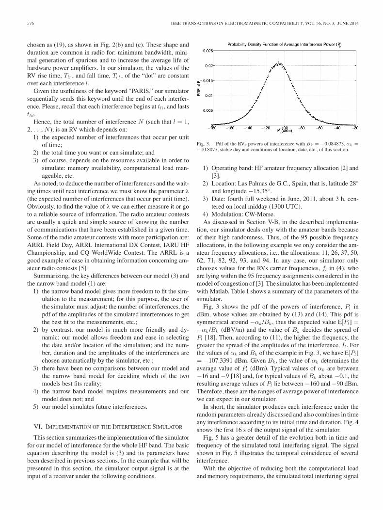
This section will present some statistical measures performedon the simulated total interfering signal from the previous sec-tion. Its purpose is confirm the random characteristics imposedon the simulated signal and also its possible future comparisonto actual measurements statistics in an “ARRL Field Day.” InFig. 6, we can observe the evolution in time and frequency ofthe simulated total interfering signal during 0.5 s.

In Fig. 6, we can see some important characteristics:1) possibility of large differences of power between the vari-

ous interference as expected according to their power pdf(see Fig. 3);

2) some degree of continuity in the time domain if all in-dividual interferences are superimposed, even though theevolution of Morse code for the keyword “PARIS” in indi-vidual interference shows a remarkable absence of carrier(56%), see Figs. 2 and 5;

3) impulsivity in the frequency domain, although the carrierfrequencies are constant for each interference these spec-tral components are absent for about 56% of the durationof each interference; and

Fig. 6. Time evolution of signal spectrum for the simulated total interferingsignal. The frequency resolution is 8192 Hz. For this time interval the maxi-mum power was found to be −72.7116 dBm at a frequency of −2.2856 MHz(14.2144 MHz in RF).

4) the width (time duration) of each “dot” remains constantin each interference because it is assumed that for eachcommunication both interlocutors have the same Morsecode speed and, therefore, the same width of “dot.”

A. Amplitude Probability Distribution (APD)

The APD succinctly express the probability that a signalamplitude exceeds a threshold. The APD provides informa-tion about an interference signal to estimate the performancedegradation of a victim receiver [22].

In this paper, APDs are plotted on a Rayleigh probabilitygraph [22]. In this paper, the axes of the representation of APDrepresent the power of the decimated I–Q interference signalin dB above k·T0 ·B versus the percent-of-time the power isexceeded. The power k·T0 ·B is the thermal noise present in everyreceiver. In this case, the bandwidth chosen for the thermal noiseis 100 Hz which coincides with the IF filter of some commercialreceivers.

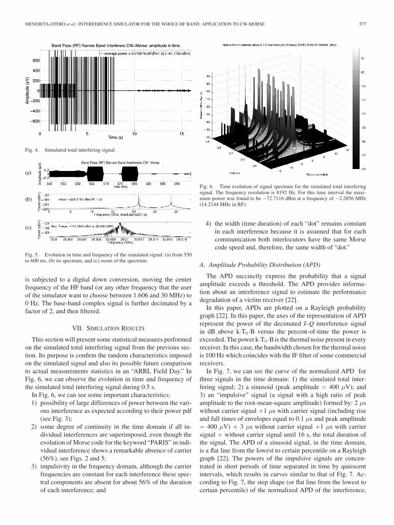
In Fig. 7, we can see the curve of the normalized APD forthree signals in the time domain: 1) the simulated total inter-fering signal; 2) a sinusoid (peak amplitude = 400 μV); and3) an “impulsive” signal (a signal with a high ratio of peakamplitude to the root-mean-square amplitude) formed by: 2 μswithout carrier signal +1 μs with carrier signal (including riseand fall times of envelopes equal to 0.1 μs and peak amplitude= 400 μV) + 3 μs without carrier signal +1 μs with carriersignal + without carrier signal until 16 s, the total duration ofthe signal. The APD of a sinusoid signal, in the time domain,is a flat line from the lowest to certain percentile on a Rayleighgraph [22]. The powers of the impulsive signals are concen-trated in short periods of time separated in time by quiescentintervals, which results in curves similar to that of Fig. 7. Ac-cording to Fig. 7, the step shape (or flat line from the lowest tocertain percentile) of the normalized APD of the interference,


Fig. 7. Normalized APD for: the simulated total interfering signal, a sinusoidand an “impulsive” signal, in the time domain.

Fig. 8. Normalized APD for: the simulated total interfering signal, a sinusoidand an “impulsive” signal, in the frequency domain.

in the time domain, implies a shape similar to the sinusoidal.Although individual interferences contain a 56% average per-centage of nonsignal, this result is expected because there aremany individual interferences that overlap in time, see Figs. 4,5, and 6.

In Fig. 8, we can see the curve of the normalized APD of thethree signals mentioned, in the frequency domain. ComparingFigs. 7 and 8, we see that the APD of the sinusoid in the timedomain, is very different from the APD of the sinusoid in thefrequency domain. The same happens with the “impulsive” sig-nal. This is expected because the bandwidths associated witheach of these signals (very large in the case of the “impulsive”signal).

Both Figs. 7 and 8 indicate an interference APD closest to theAPD for the sinusoid than for the “impulsive” signal. As shownin Fig. 6, the impulsive behavior seems higher in the frequencydomain than in the time domain since in the frequency domainthere is no overlap between individual interferences. Namely,this higher impulsiveness in the frequency domain is due to thefact that frequencies of the individual interferences are relativelyfar from one another, and also to that the individual interferencesare present only for short periods of time in which there is carrier.However, in Figs. 7 and 8, the APD of the total interferingsignal not clearly shows that the impulsiveness is higher in thefrequency domain than in the time domain. This is because the

Fig. 9. Normalized LCD of the voltage envelope for: the simulated totalinterfering signal, a sinusoid and an “impulsive” signal, in the time domain.

APD is not a good indicator of the arrival times of the signalamplitudes, as in the case of the level crossing statistics, someof which are discussed in the following section.

B. Level Crossing Statistics

Computation of BERs in many modern digital receivers re-quires statistics describing the time of arrival of signal ampli-tudes [22]. Moreover, due to the nature of our simulated signal,there may be a large amount of carrier absence, about 56% (seeFig. 2), or a large number of overlapping small amplitude values(see Figs. 4, 5, and 6). This would result in pdfs for the envelopesof voltage and power with narrow and sharp peaks due to the val-ues equal to zero. These pdfs may mask the distributions presentin the signal. Using level crossings statistics we can overcomethis inconvenience by setting a minimum threshold of zero. Inthis way, we only take into account how much the values exceedthis threshold. This type of situation is common not only forCW-Morse signals but for pulsed signals and impulsive noise.

To study the envelope values we have in the simulated signal,we used the level crossing distribution (LCD). The LCD isthe distribution of the number of upgoing crossings throughsome levels or thresholds of the signal envelope. Fig. 9 showsa representation of the normalized LCD for the three signalsdiscussed in the previous section, and it can be appreciated themost common envelope levels in the interference (see Figs. 4,5, and 6) as well as its great variability (a high value of Max.LCD) with respect to the sinusoid and the “impulsive” signal.

To study how long it takes from the moment the envelopeexceeds a threshold to when it goes above it again, we use theaverage cross duration (ACD). For each threshold, the ACD isthe average of the upgoing crossing times. Fig. 10 shows a repre-sentation of the normalized ACD for the three signals discussedin the previous section. In Fig. 10, the first threshold value cor-responding to 0 μV is not represented, for better viewing of thegraph. However, its value, which coincides with the maximumvalue of the ACD, is displayed in the legend of Fig. 10. There-fore, these minimum values of envelope are present much longerthan the rest of envelope values. As in the case of the LCD, themaximum value of the ACD and their distribution are different


Fig. 10. Normalized ACD of the voltage envelope for: the simulated totalinterfering signal, a sinusoid and an “impulsive” signal, in the time domain.

Fig. 11. LCD of the power envelope for the simulated total signal.

from those corresponding to the sinusoid and to the “impulsive”signal.

In Fig. 10, the abrupt changes in value of the ACD to certainthresholds are due to the superposition of individual interfer-ences with very different values for the durations of the levelcrossings (in this case, most with small durations). Thus, in thecase of CW-Morse interferences, it is an indication that variousindividual interferences exist simultaneously with very differenttransmission speeds, i.e., with very different values of WPM.

Fig. 11 shows the LCD of the power envelope in the timedomain. The aim is to compare with the pdf of the individ-ual interference powers, as shown in Fig. 3. In Fig. 11 can benoticed that the most frequent value is −87.3495 dBm, being−107.3391 dBm the expected value for the pdf of Fig. 3. Thishigher power value is to be expected since the LCD of Fig. 11is for the total interfering signal, while the values in Fig. 3are the average power of each individual interference during itslifetime.

VIII. FUTURE WORK

It is evident that the validity of the implemented simulatormust be proved by comparing the results of the simulation withreal interference measurements. The tests of the model should

include amateur radio, using: CW-Morse, SSB and even RadioTeleTYpe. The tests should also include other kind of commonusers in the HF band, such as AM stations and the military HFradio stations (using, for example, M-ary PSK). There is a highprobability that power line telecommunications would causeincreased noise levels at sensitive receiver sites given the exist-ing and projected market penetration [23]. Therefore, the testsshould also include possible interference of power line com-munications systems (using, for example, orthogonal frequencydivision multiplexing).

Future work should include congestion models including up-dated forecasts based on time of day, beyond our weekly modelthat was focused on noon and midnight. Also, it must be re-membered that the model of congestion has been developed onmeasurements taken in Northern Europe. It would be desirablefor the models of congestion also to include long-range commu-nications using near vertical incidence (NVIS), i.e., monopolehigh angles.

A possible application of the interference simulator beyondHF may be in the global positioning system (GPS) band. Asin the case of HF, the simulator would be a tool for evaluatingcommunication systems (GPS in this case) as well as potentialnew methods to combat interference.

IX. CONCLUSION

An interference simulator for the whole HF band (1.606–30 MHz) has been modeled and implemented. The simulatorgenerate interfering signals that can be found in a given fre-quency allocation, in a given time (past, present, or future) andfor a given location. The simulator has been used to simulateCW-Morse interference of the “ARRL Field Day 2011.” It hashighlighted some statistical measures useful in the analysis ofinterferences, especially in the case of CW-Morse interferences.

Our most important original contributions are as follows.1) To create a new model and simulator, we used jointly and

in detail two existing independent models: a congestionmodel and a model of narrowband interference. Basically,the user of the simulator selects the date and location aswell as the modulation assigned to each frequency alloca-tion. So that our model, to generate the simulated signalfor all the HF frequency allocations, provide at each in-stant, the number of interferences, their frequencies, theiramplitudes, their temporal onset, duration, etc.

2) Our model does not require measurements.3) As a result, our simulator is characterized by its ease of

use and the freedom it offers to choose scene (modulation,location, week, year, etc.).

4) In addition, we have defined a generic modulating functionand the conditions to model a “contact” CW-Morse, whomeets the usual standards of contest.

5) Consequently, our interference model in conjunction withthe CW-Morse modulating function designed, it results ina specific model for CW-Morse amateur contests. The ma-jor radio amateur contests can be a good scene to evaluatea communications system subjected to a high degree of“interferences.”


REFERENCES

[1] ITU, Radio Regulations. Geneva, Switzerland: ITU Electronic Publishing,2012, vol. 1, Article 2.

[2] Radio Regulations Revised Table of Frequency Allocations and AssociatedTerms and Definitions, ITU WARC 1979, (HMSO 1980), 1979.

[3] L.V. Economou, H. Haralambous, C. A. Pantjairos, P. R. Green, G. F. Gott,P. J. Laycock, M. Broms, and S. Boberg, “Models of HF spectral occu-pancy over a sunspot cycle,” IEE Proc. Commun., vol. 152, no. 6, pp. 980–988, Dec. 2005.

[4] International Telecommunications Union, “Status summary of radio am-ateurs & amateur stations of the world,” (2012). [Online]. Available:http://www.iaru.org

[5] ARRL, The National Association for Amateur Radio, Newington, CT,USA, (2012). [Online]. Available: http://www.arrl.org

[6] International Telecommunication Union, “Radio noise,” RecommendationITU-R P.372–10, Oct. 2009.

[7] H. C. Haralambous, L. Economou, C. A. Pantjiaros, and L. Christofi,“Monitoring of HF spectral occupancy in Cyprus,” in Proc. IEE 11thIET Int. Conf. Ionospheric Radio Syst. Techn., Apr. 2009, pp. 1–4.

[8] J. F. Mastrangelo, J. J. Lemmon, L. E. Vogler, J. A. Hoffmeyer, L. E. Pratt,and C. J. Behm, “A new wideband high frequency channel simulationsystem,” IEEE Trans. Commun., vol. 45, no. 1, pp. 26–34, Jan. 1997.

[9] E. Mendieta-Otero, I. Perez-Alvarez, S. Zazo-Bello, H. Santana-Sosa,J. Lopez-Perez, and I. Raos, “Implementation and comparison of a wide-band HF noise and interference simulator,” in Proc. IEE 10th IET Int.Conf. Ionospheric Radio Syst. Techn., 2006, vol. 2006, pp. 143–146.

[10] J. Laxmark, “An interference simulator for performance evaluation ofadaptive HF systems,” in Proc. IEEE Military Commun. Conf. Rec. Com-mun. Move, 1993, vol. 1, pp. 62–66.

[11] H. M. Hall, “A new model of ‘Impulsive’ phenomena: Application toatmospheric-noise communication channels,” Electron. Lab., StanfordUniv., CA, USA, Tech. Rep. 3412–8 and 7050-7, SU-SEL-66-052, Aug.1966.

[12] D. Middleton, “Non-gaussian noise models in signal processing fortelecommunications: New methods and results for class A and class Bnoise models,” IEEE Trans. Inform. Theory, vol. 45, no. 4, pp. 1129–1149, May 1999.

[13] G. Bark, “Spread-spectrum communications in the interference-limitedHF band,” Ph.D. Thesis, Dept. of Signals, Sensors and Systems, RoyalInst. of Technology, Stockholm, Sweden, Oct. 1997.

[14] H. Haralambous and H. Papadopoulos, “24-hour neural network conges-tion models for high-frequency broadcast users,” IEEE Trans. Broadcast.,vol. 55, no. 1, pp. 145–154, Mar. 2009.

[15] H. Haralambous and H. Papadopoulos, “Short-term forecasting of thelikelihood of interference to groundwave users in the lowest part of theHF spectrum,” in Proc. IEEE 4th Int. Conf. Intell. Syst., 2008, vol. 2, pp.17–22.

[16] World Data Centre for Solar-Terrestrial Physics, Rutherford AppletonLab., Chilton, Oxfordshire, UK. (2012). [Online]. Available: http://www.ukssdc.ac.uk/cgi-bin/wdcc1/secure/geophysical_parameters.pl

[17] U.S. Dept. of Commerce, NOAA (National Oceanic and AtmosphericAdministration), Space Weather Prediction Center (SWPC), Boulder, CO,USA. (2012). [Online]. Available: http://www.swpc.noaa.gov/SolarCycle

[18] G. Bark, “Performance comparison of spread-spectrum methods on aninterference-limited HF channel,” IEE Proc. Commun., vol. 146, no. 1,pp. 23–28, 1999.

[19] International Telecommunication Union, “Miscellaneous abbreviationsand signals to be used for radiocommunications in the maritime mobileservice,” Recommendation ITU-R M.1172, 1995.

[20] International Telecommunication Union, “International morse code,” Rec-ommendation ITU-R M.1677–1, Oct. 2009.

[21] A. D. Spaulding and G. H. Hagn, “On the definition and estimation ofspectrum occupancy,” IEEE Trans. Electromagn. Compat., vol. EMC-19,no. 3, pp. 269–280, Aug. 1977.

[22] W. A. Kissick, “The temporal and spectral characteristics of ultrawidebandsignal,” NTIA Report TR-01-383, Jan. 2001.

[23] A. Chubukjian, J. Benger, R. Otnes, and B. Kasper, “Potential effectsof broadband wireline telecommunications on the HF spectrum,” IEEECommun. Mag., vol. 46, no. 11, pp. 49–54, Nov. 2008.

Eduardo Mendieta-Otero was born in La Habana,Cuba, in 1966. He received the B.Sc. (Hons.) de-gree in electronic equipment, the B.Sc. (Hons.) de-gree in radio communication, and the M.S. degree intelecom engineering from the University of Las Pal-mas de Gran Canaria (ULPGC), Las Palmas de GranCanaria, Spain, in 1992, 1994, and 2001, respectively.

He joined the ULPGC as an Associate Professorin 1994. From 2006 to 2010, he was a member ofthe Technological Centre for Innovations in Commu-nications. From 2010, he has been a member of the

Institute for Technological Development and Innovation in Communications,Las Palmas de Gran Canaria. His research interests mainly include the field ofsignal processing for radio communications.

Ivan A. Perez-Alvarez (M’89) was born in GranCanaria, Spain, in 1965. He received the M.S. degreein telecom engineering and Dr.Eng. degree from theUniversidad Politecnica de Madrid, Spain, in 1990and 2000, respectively.

From 1989 to 1997, he was in Europea deComunicaciones S.A. and Telefonica Sistemas S.A.,where he was a Member Staff of the Special ProjectsDepartment and working in the Digital Signal Pro-cessing Group. He was involved in the design ofHF/VHF/UHF digital communications systems for

the Spanish Ministry of Defence. He joined the ULPGC, Spain, as an AssociateProfessor in 1998. In 2006, he was Head of CeTIC until 2010 and at the presentis the Vice-Director of the Institute for Technological Development and Innova-tion in Communications, Spain. His research interests mainly include the fieldof signal processing for radio communications.

Baltasar Perez Dıaz was born in Tenerife, Spain, in1975. He received the M.S. degree in telecom en-gineer from the University of Las Palmas de GranCanaria, Spain, in 2005.

He is currently working as a Research Assistant forthe Institute for Technological Development and In-novation in Communications, Spain, in hardware de-velopments on HF broadband radiocommunications.His research interests include broadband radiocom-munications, RF subsystems, coupled-oscillator ar-rays on microwave bands and millimetre band radar.

Interference Simulator for the Whole HF Band: Application to CW-Morse

Documents

Transcript of Interference Simulator for the Whole HF Band: Application to CW-Morse